Embed Size (px)
Citation preview
Oxford University Engineering Library Technical Report OUEL 2250/02
The Effects of Translational Misalignment in the Self-Calibrationof Rotating and Zooming Cameras
Eric Hayman∗ and David W. Murray†
∗ Royal Institute of Technology (KTH)Computational Vision and Active Perception Laboratory (CVAP)
Dept. of Numerical Analysis and Computer ScienceS-100 44 Stockholm
† Department of Engineering ScienceUniversity of Oxford
Parks RoadOxford OX1 3PJ
March 6, 2002, revised September 27th 2002
This work was carried out in the Department of Engineering Science, University of Oxford, under GrantGR/L57668 from the UK Engineering and Physical Science Research Council. E. Hayman’s doctoralstudies were supported by the Norwegian Research Council.
Abstract
Algorithms for self-calibrating cameras whose changes in calibration parameters are confined to rotationand zooming are useful since many real-world imaging situations do not permit translations — considerfor instance cameras mounted on tripods and desk- or wall-mounted active heads. In practice, however,the assumption of pure rotation is often violated because the optic centre of the camera and the rotationcentre do not completely coincide. This work determines how such misalignments affect the estimation ofthe camera focal length. Expressions for the errors in focal length and recovered rotations are derived,and results are confirmed with experiments on synthetic data. We show that the approximation of purerotation is indeed sufficient in many cases, especially since other sources of error such as noise andparticularly radial distortion tend to be more detrimental.
Index Terms: Self-calibration, zoom lenses, rotating cameras
1 Introduction
The self-calibration of cameras which may rotate and possibly zoom, but not translate, has been a topic ofsignificant interest in the computer vision community in recent years [6, 3, 2, 12, 13, 14]. This researchhas often been motivated by practical applications such as generating cylindrical or spherical mosaicsfrom a single viewpoint or augmenting original film footage with computer graphics imagery when thecamera motion is described by a pure pan and/or tilt. Furthermore, there are currently several researchprojects concerning reconstructing sports highlights in 3D. Such events are often covered by camerasmounted on tripods, and a first step in the reconstruction would be to self-calibrate the cameras from astatic background, most obviously the sports pitch.
However, in many systems the assumption that the motion is a pure rotation about the camera’s opticcentre is only an approximation. Consider for instance a camera mounted on top of a tripod. The rotationcentre is typically a good few centimeters below the optic centre of the camera, and in addition thereis no guarantee that the pan and tilt axes intersect. The matter is further complicated with zoom lensessince, even without rotations of the camera, the optic centre may move by as much as a few centimetersalong the optic axis as the lens is zoomed.
Physical intuition suggests that these effects should be negligible if the distance to the scene is large incomparison with the movement of the optic centre: we would expect some reliance on the dimension-less ratio between this movement and scene depth. In this paper we derive analytic expressions for thisdependency, and support our findings in experiments using simulated data with no added noise. Theconclusion is that the approximation of pure rotation is indeed a good one in many practical scenarios.It is assumed that skew is zero and aspect ratio is unity, and that the principal point is known. Priorknowledge concerning skew and aspect ratio is certainly very reasonable to assume in practical appli-cations, and we choose not to solve for the principal point partly to keep the analysis simple, but alsobecause recovering these parameters in a self-calibration can be ill-conditioned and also destabilizing forestimating focal length [9]. Thus we only solve for focal length, although this parameter is allowed tovary between frames. We also consider the effect on the recovered motion of the camera.
We provide two alternative methods to derive these results. The first is based on discrete motion, astypically used in self-calibration algorithms. The second considers instantaneous image velocities andallows a quick and intuitive analysisindependent of self-calibration algorithm for first order approxima-tions of small rotations and for zero noise. Expressions are initially derived for self-calibration from justtwo frames, but are subsequently extended to an arbitrary number of images.
These misalignment effects have largely been neglected in previous literature on rotational camera cali-
1

bration, and there is especially a lack of quantitative results. Stein [15] produced an expression for errorin recovered focal length when calibrating an active head from known rotations. In work simultaneousto and independent of ours1, Wanget al. [19] considered the case of the intrinsic parameters remain-ing unchanged throughout the sequence. In addition to analyzing fully uncalibrated cameras, they alsodealt with partially calibrated cameras, incorporating conditions of known principal point, aspect ratioand/or skew. A major difference is that they considerrandom translations caused for instance by shakyhand-held operation whereas we consider thesystematic ones for cameras mounted on tripods and activeheads, as was discussed above.
The rest of this paper is organized as follows. In Section 2 we briefly review literature on the self-calibration of rotating cameras before predicting in Sections 3 and 4 how the algorithms are affectedby misalignments between the optic and rotation centres. Section 5 verifies these predictions with ex-periments on synthetic data. In the discussion in Section 6 these errors are compared with those fromother common sources such as uncompensated radial distortion and random Gaussian noise in the featuredetection, demonstrating that misalignments are unlikely to be the major cause of poor calibration. Sec-tion 7 demonstrates that our analysis is not affected by the incorporation of supplementary constraintsconcerning the camera returning to its original position. Finally, Section 8 discusses why constraintsindependent of translation for fixed focal length in [19] extend poorly to zoom lenses and cannot beused with small rotations, and Section 9 provides a preliminary investigation into calibration from largerrotations.
2 Self-calibration from pure rotation: review
The standard pinhole camera projection model in homogeneous coordinates isx = PX whereP is the3 × 4 projection matrixP = K(R t). K contains the intrinsic parameters, and in this work is assumed totake the simple form
K =
f 0 0
0 f 00 0 1
wheref is the focal length and the other intrinsic parameters are assumed known. If the motion of thecamera is a pure rotation about its optic centre, the translation vectort can be dropped, and the projectionequation simplifies toxi = KiRi (X Y Z) . Different images,i andj, taken from the same rotatingcamera relate to each other by homographiesHij
xj = Hijxi, Hij = KjRjR−1i K−1
i = KjRijK−1i . (1)
The inter-image homographiesHij may be calculated directly from image measurements, for instancefrom point or line correspondences [7], or directly from greyvalues by minimizing the brightness con-stancy constraint [1]. EliminatingRij from equation (1) yields(
KjKj)
= Hij
(KiKi
)Hij
. (2)
Thus, given the homographies,Hij , equation (2) provides constraints on the intrinsic parameters. Thisequation is also known as the infinite homography constraint.
Hartley demonstrated in [6] the self-calibration of a rotating camera with constant intrinsic parameterswith a simple, linear method. More recently, de Agapito and co-workers [3, 2] and Seo and Hong[12, 13] have provided algorithms for cameras with zoom lenses. When only solving for focal length,
1Our work first appeared in [8].
2
equation (2) takes a simple form giving five equations to solve for the focal length before and after themotion, denoted byf ′
0 andf ′1 respectively2,
f ′02 (h11h21 + h12h22) = −h13h23 (3)
f ′02 (h11h31 + h12h32) = −h13h33 (4)
f ′02 (h21h31 + h22h32) = −h23h33 (5)
f ′12 =
f ′02(h2
11 + h212) + h2
13
f ′02(h2
31 + h232) + h2
33
(6)
f ′12 =
f ′02(h2
21 + h222) + h2
23
f ′02(h2
31 + h232) + h2
33
(7)
wherehkl is element(k, l) of the homographyH. In this paper we distinguish between theveridical focallengthsf0, f1 and theestimated quantitiesf ′
0, f′1 through the use of dashes.
3 Force-fitting rotational motion
A typical self-calibration scheme can be split into two main stages. The first concerns obtaining thehomographies. Typically, corner features are detected and matched between image pairs, and homogra-phies are fitted using robust methods such as RANSAC [5, 17]. In the second stage the homographiesare fed into an algorithm based on equation (2).
Consider now how such a technique copes when small translations are also present. In the first stagea homography is force-fit between image pairs. A homography is not only the appropriate descriptionof the two-view geometry under pure rotation for a general scene, but also under general motion for aplanar scene, in which case the homography is given by
Hij = Kj
(Rij +
1di
tijni)K−1
i (8)
wheretij = (tX tY tZ) is the translation of the camera’s optic centre andni the unit normal of theplane. The equation of the plane isni
X = di wheredi is the perpendicular distance to the plane fromthe optic centre. SinceHij in equation (8) is more general than that in equation (1), in the first stage ofself-calibration some effective scene plane is found. In the second stage a purely rotational motion isforce-fit to this homography.
In much of the following we will assume that the scene in front of the camera may be modelled by afronto-parallel plane at distanced to the camera since this will, in fact, be roughly true in many practicalcases. This requirement will, however, be relaxed when relevant. Also, we largely assume that thetranslation of the camera is caused by a fixed length rotation armq such that
t = Rq − q .
From now on the subscriptsi andj will be dropped when it is clear which frame quantities refer to.
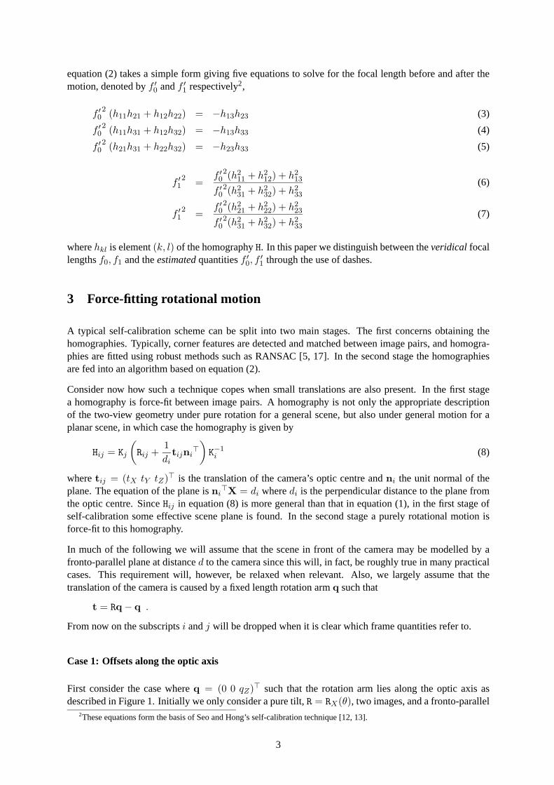
Case 1: Offsets along the optic axis
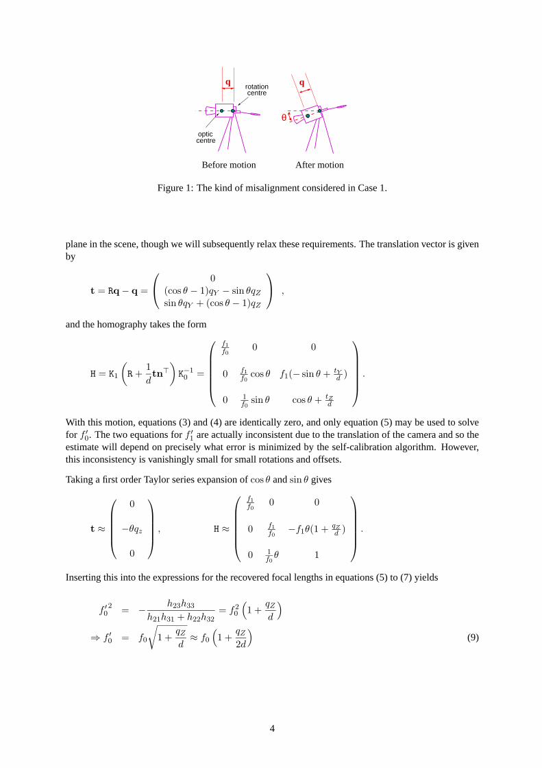
First consider the case whereq = (0 0 qZ) such that the rotation arm lies along the optic axis asdescribed in Figure 1. Initially we only consider a pure tilt,R = RX(θ), two images, and a fronto-parallel
2These equations form the basis of Seo and Hong’s self-calibration technique [12, 13].
3
q
opticcentre
θ
After motion
rotationcentre
Before motion
q
Figure 1: The kind of misalignment considered in Case 1.
plane in the scene, though we will subsequently relax these requirements. The translation vector is givenby
t = Rq − q =
0
(cos θ − 1)qY − sin θqZ
sin θqY + (cos θ − 1)qZ
,
and the homography takes the form
H = K1
(R +
1dtn
)K−1
0 =
f1
f00 0
0 f1
f0cos θ f1(− sin θ + tY
d )
0 1f0
sin θ cos θ + tZd
.
With this motion, equations (3) and (4) are identically zero, and only equation (5) may be used to solvefor f ′
0. The two equations forf ′1 are actually inconsistent due to the translation of the camera and so the
estimate will depend on precisely what error is minimized by the self-calibration algorithm. However,this inconsistency is vanishingly small for small rotations and offsets.
Taking a first order Taylor series expansion ofcos θ andsin θ gives
t ≈
0
−θqz
0
, H ≈
f1
f00 0
0 f1
f0−f1θ(1 + qZ
d )
0 1f0
θ 1
.
Inserting this into the expressions for the recovered focal lengths in equations (5) to (7) yields
f ′02 = − h23h33
h21h31 + h22h32= f2
0
(1 +
qZ
d
)
⇒ f ′0 = f0
√1 +
qZ
d≈ f0
(1 +
qZ
2d
)(9)
4
f ′12 =
f ′02(h2
11 + h212) + h2
13
f ′02(h2
31 + h232) + h2
33
=f20
(1 + qZ
d
) f21
f20
f20
(1 + qZ
d
)θ2
f20
+ 1≈ f2
1
(1 +
qZ
d
)
⇒ f ′1 = f1
√1 +
qZ
d≈ f1
(1 +
qZ
2d
)(10)
f ′12 =
f ′02(h2
21 + h222) + h2
23
f ′02(h2
31 + h232) + h2
33
=f20
(1 + qZ
d
) f21
f20
+ f21 θ2
(1 + qZ
d
)f20
(1 + qZ
d
)θ2
f20
+ 1≈ f2
1
(1 +
qZ
d
)
⇒ f ′1 = f1
√1 +
qZ
d≈ f1
(1 +
qZ
2d
)(11)
where both equations (6) and (7) forf ′1 provide the same result. Expressions inθ2 were neglected, and
a binomial expansion of the expression in the square root was performed, assuming thatqZ/d 1. Wenote the following:
• The error in focal length is proportional to the length of the rotation arm and inverse proportionalto the distance to the scene.
• There is no dependency on the angle of rotation,θ.
Inserting the expressions forf ′0 andf ′
1 into K0 andK1, the rotation matrix (up to scale in the first line) isthen given by
R = K−11 HK0 =
h11 h121f ′0h13
h21 h221f ′0h23
f ′1h31 f ′
1h32f ′1
f ′0h33
=
1 0 0
0 1 −θ 1+qZ/d1+qZ/(2d)
0 θ(1 + qZ
2d
)1
≈
1 0 0
0 1 −θ(1 + qZ
d
) (1 − qZ
2d
)0 θ
(1 + qZ
2d
)1
≈
1 0 0
0 1 −θ(1 + qZ
2d
)0 θ
(1 + qZ
2d
)1
.
In developing element (2,3) a binomial expansion(1 + a)−1 ≈ 1 − a is used sincea 1, and secondorder terms are ignored. The recovered rotation,θ′, is about thex-axis and is
θ′ = θ(1 +qZ
2d). (12)
5
The error in the estimate of camera rotation is therefore also proportional to|q| and inverse proportionalto d.
Since the expressions forf ′0, f ′
1 andθ′ are independent of the amount by which the camera rotated, theystill hold when self-calibrating from sequences containing more than two images, provided the effectivescene plane remains the same. Furthermore, a similar analysis shows that the same expressions forf ′
0,f ′1 andθ′ are obtained also when the motion is a pure pan or a combination of pan and tilt. Experiments
confirming these findings are described in Section 5. Additionally, rotations aboutz may be incorporatedprovided some tilt or pan is still present, pure rotation aboutz is fundamentally degenerate for focallength estimation.
It is also interesting to investigate how important the assumption of a fronto-parallel plane is. We there-fore permit a general plane normaln = (nX nY nZ) and also extend the analysis to higher orderapproximations ofcos θ andsin θ. The working is provided in Appendix A, but the main result is
f ′0 = f0
(1 +
qZ
2dnZ +
qZ
d
3θ
4nY
)+ O(3) , (13)
that is, the additional error in focal length estimation due to non-zeronY is second order sinceqZ/dandθ are small. In fact, ifnY 1, i.e. the effective scene plane is roughly fronto-parallel, then thisadditional error is a third order term. Similar expressions hold forf ′
1 and are provided in the Appendix.The independence ofnX in equation (13) is of limited practical interest since it is highly unlikely thatthe effective scene plane has the orientationn = (1 0 0).
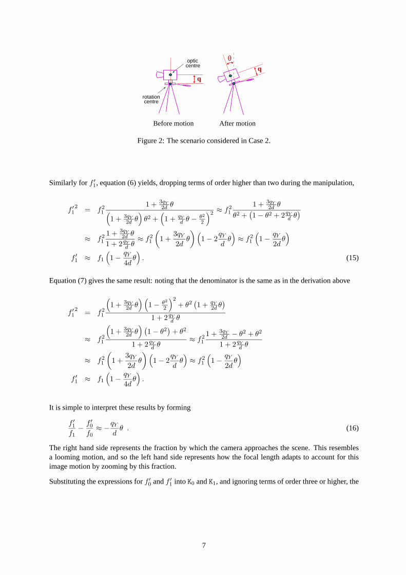
Case 2: Offsets parallel to the image plane
Consider also the case ofq = (0 qY 0), as illustrated in Figure 2. Taking a second order approximation,the translation is
t = Rq − q =
0
− θ2
2 qY
qY θ
.
and the homography is given by
H ≈
f1
f00 0
0 f1
f0
(1 − θ2
2
)−f1θ
(1 + qY
2d θ)
0 θf0
1 + qYd θ − θ2
2
.
Computingf ′0 from equation (5) yields
f ′02 = f2
0
(1 + qY
2d θ) (
1 + qYd θ − θ2
2
)(1 − θ2
2 )≈ f2
0
(1 +
3qY
2dθ − θ2
2
(1 +
qY
dθ)) (
1 +θ2
2
)
≈ f20
(1 +
3qY
2dθ
)+ O(3)
f ′0 ≈ f0
(1 +
3qY
4dθ
)+ O(3). (14)
6
centrerotation
opticcentre
θq
Before motion After motion
q
Figure 2: The scenario considered in Case 2.
Similarly for f ′1, equation (6) yields, dropping terms of order higher than two during the manipulation,
f ′12 = f2
1
1 + 3qY2d θ(
1 + 3qY2d θ
)θ2 +
(1 + qY
d θ − θ2
2
)2 ≈ f21
1 + 3qY2d θ
θ2 +(1 − θ2 + 2 qY
d θ)
≈ f21
1 + 3qY2d θ
1 + 2 qYd θ
≈ f21
(1 +
3qY
2dθ
) (1 − 2
qY
dθ)≈ f2
1
(1 − qY
2dθ)
f ′1 ≈ f1
(1 − qY
4dθ)
. (15)
Equation (7) gives the same result: noting that the denominator is the same as in the derivation above
f ′12 = f2
1
(1 + 3qY
2d θ) (
1 − θ2
2
)2+ θ2
(1 + qY
2d θ)
1 + 2 qYd θ
≈ f21
(1 + 3qY
2d θ) (
1 − θ2)
+ θ2
1 + 2 qYd θ
≈ f21
1 + 3qY2d − θ2 + θ2
1 + 2 qYd θ
≈ f21
(1 +
3qY
2dθ
) (1 − 2
qY
dθ)≈ f2
1
(1 − qY
2dθ)
f ′1 ≈ f1
(1 − qY
4dθ)
.
It is simple to interpret these results by forming
f ′1
f1− f ′
0
f0≈ −qY
dθ . (16)
The right hand side represents the fraction by which the camera approaches the scene. This resemblesa looming motion, and so the left hand side represents how the focal length adapts to account for thisimage motion by zooming by this fraction.
Substituting the expressions forf ′0 andf ′
1 into K0 andK1, and ignoring terms of order three or higher, the
7
rotation matrix is then given by
R = K−11 HK0 =
h11 h121f ′0h13
h21 h221f ′0h23
f ′1h31 f ′
1h32f ′1
f ′0h33
=
1 0 0
0 1 − θ2
2 −θ(1 + qY
2d θ) (
1 − 3qY4d θ
)
0 θ(1 − qY
4d θ) (
1 − θ2
2 + qYd θ
) (1 − qY
d θ)
≈
1 0 0
0 1 − θ2
2 −θ(1 + qY
2d θ − 3qY4d θ
)
0 θ(1 − qY
4d θ)
1 − θ2
2 + qYd θ − qY
d θ
≈
1 0 0
0 1 − θ2
2 −θ(1 − qY
4d θ)
0 θ(1 − qY
4d θ)
1 − θ2
2
.
Thus the recovered rotation,θ′, is about thex-axis and is
θ′ = θ(1 − qY
4dθ). (17)
The error in parameters is again proportional to the length ofq and inverse proportional to scene depth,although now there is also a dependency on the angle of rotationθ. Due to this dependency onθ, as longas the rotation of the camera is small, withq = (0 qY 0) errors in focal length are much less severethan in Case 1 whereq = (0 0 qZ).
The dependency off ′0 on θ in equation (14) implies that introducing further images into the self-
calibration algorithm will change the estimate off ′0, and thus also the recovered rotations. However,
the relative change in focal length(f ′1/f1) − (f ′
0/f0) is still equal to−(qY θ)/d.
It is straightforward to extend the analysis to an effective scene plane with arbitrary orientation,n =(nX nY nZ), yielding the homography
H ≈
f1
f00 0
−f1
f0
θ2
2qYd nX
f1
f0
(1 − θ2
2
(1 + qY
d nY
)) −f1θ(1 + qY
2d θ)nZ
− 1f0
θ qYd nX
θf0
(1 + qY
d nY
)1 + qY
d θnZ − θ2
2
.
We obmit the working here since the result is, in fact, quite intuitive. Equation (5) gives
f ′0 ≈ f0
(1 +
3qY
4dθnZ − qY
2dnY
)+ O(3)
8
whereas equations (6) and (7) both yield
f ′1 ≈ f1
(1 − qY
4dθnZ − qY
2dnY
)+ O(3) .
In addition to the calibration errors attributed tonZ , there is now an additional error which is proportionalto nY and independent ofθ. This term is exactly what is predicted by Case 1 sincenY = 0 implies thatthere is now significant camera translation parallel to the planar surface rather than just perpendicular toit. Similarly, calibration errors caused by a misalignment ofq = (0 qY qZ) can be decomposed intothe same two components described by Cases 1 and 2 respectively. Summarizing these findings, errorsin focal length are most severe when there is a component ofq which is parallel to the plane normal.
With a misalignment ofq = (0 qY 0) a pure panning motion does not induce any translations of theoptic centre, and focal length estimation is free of errors. With tilt combined with pan, equation (16) stillholds. Again, experiments confirming this analysis are given in Section 5. Similar results are obtainedfor pure pan if the misalignment isq = (qX 0 0).
Rotations aboutz now induce camera translations which cause further errors in focal length computation.However, this translation does not involve any looming motion, so the relative change in focal length isstill given by equation (16). We defer a discussion of this topic to Section 4.
Case 3: Motion along the optic axis due to zoom
We now consider the case where the optic centre moves along the optic axis as the lens zooms,t =(0 0 tZ) while the camera rotates by a small amount aboutx and/ory, possibly in combination withrotations aboutz. This case is very similar to Case 2 although the translation is now decoupled from therotation of the camera. For the analysis we assume that the rotation is just about thex-axis, as previously.The homography is then given by
H ≈
f1
f00 0
0 f1
f0
(1 − θ2
2
)−f1θ
0 θf0
1 − θ2
2 + tZd
.
As before equation (5) is used to obtain an estimate of the focal length in frame 0
f ′02 = f2
0
θ(1 − θ2
2 + tZd
)θ(1 − θ2
2
) ≈ f20
(1 +
tZd
)
f ′0 ≈ f0
(1 +
tZ2d
)
Similarly for f ′1, equation (6) yields
f ′12 = f2
1
1 + tZd(
1 + tZd
)θ2 +
(1 − θ2
2 + tZd
)2 ≈ f21
1 + tZd
θ2 + 1 − θ2 + 2 tZd
≈ f21
(1 +
tZd
) (1 − 2
tZd
)≈ f2
1
(1 − tZ
d
)
f ′1 ≈ f1
(1 − tZ
2d
)
9
Equation (7) gives the same result: noting that the denominator is the same as in the derivation above
f ′12 = f2
1
(1 + tZ
d
) (1 − θ2
2
)2+ θ2
1 − 2 tZd
≈ f21
(1 + tZ
d
) (1 − θ2
)+ θ2
1 − 2 tZd
≈ f21
(1 + tZ
d
)1 − 2 tZ
d
≈ f21
(1 − tZ
d
)
f ′1 ≈ f1
(1 − tZ
2d
)
Again, the significant point is that equation (16) holds; a self-calibration algorithm includes extra zoomto accommodate the looming motion from the forward translation.
Inserting the expressions forf ′0 andf ′
1 into K0 andK1, the rotation matrix is then given by
R = K−11 HK0 =
h11 h121f ′0h13
h21 h221f ′0h23
f ′1h31 f ′
1h32f ′1
f ′0h33
=
1 0 0
0 1 − θ2
2 −θ(1 − tZ
2d
)0 θ
(1 − tZ
2d
) (1 − θ2
2 + tZd
) (1 − tZ
d
)
≈
1 0 0
0 1 − θ2
2 −θ(1 − tZ
2d
)0 θ
(1 − tZ
2d
)1 − θ2
2 + tZd − tZ
d
=
1 0 0
0 1 − θ2
2 −θ(1 − tZ
2d
)0 θ
(1 − tZ
2d
)1 − θ2
2
and so the recovered rotation,θ′, is about thex-axis and is
θ′ = θ(1 − tZ2d
). (18)
Again these errors are proportional to the dimensionless ratio|t|/d.
In practice one must question the assumption of a translation purely along thez-axis referred to the firstframe; the movement of the optic centre also gives rise to a rotation armqZ = tz, and so the results fromCase 1 should also be considered.
4 Analysis using image velocity
We now turn to the second method for deriving the errors in focal length and motion recovery. Ratherthan using discrete motions described by homographies, we consider expressions for instantaneous imagevelocity obtained by differentiating the inhomogeneous pinhole camera model equation,x = (f/Z)X,with respect to time, yielding
x =f
ZX +
f
ZX − fZ
Z2X (19)
10
where the focal lengthf is a function of time,x = (x y f) andX = (X Y Z) are expressed in cameracentred frames, and whereZ = d andX = Ω×X+V. The translational componentV = t is given byV = Ω × q if the motion is caused by a rotation about a constant length rotation arm,q. AdditionallysubstitutingX = (Z/f)x back into equation (19) then yields the image velocity
x =
x
y
=
+fΩY − yΩZ + x
f (xΩY − yΩX) + fxf + f
d (qZΩY − qY ΩZ) − xd (qY ΩX − qXΩY )
−fΩX + xΩZ + yf (xΩY − yΩX) + fy
f + fd (qXΩZ − qZΩX) − y
d (qY ΩX − qXΩY )
.
Self-calibration assuming a purely rotating camera will attempt to fit to this expression an image velocityof
x′ =
x′
y′
=
+f ′Ω′
Y − yΩ′Z + x
f ′ (xΩ′Y − yΩ′
X) + f ′xf ′
−f ′Ω′X + xΩ′
Z + yf ′ (xΩ′
Y − yΩ′X) + f ′y
f ′
.
Case 1: Offsets along the optic axis
We first consider the case whereq = (0 0 qZ). This offset will induce translations of the optic centrewhich are parallel to the image and scene planes, contributing to the image motion with a roughly uniformcomponent
x =fqZ
d
(ΩY
−ΩX
).
The values of focal length and angular velocity for the motion field of a rotating and zooming cameramust be adjusted to compensate for this additional motion. By inspection, rotation about the optic axis isunaffected, as is the relative rate of change of focal length,f/f , since this motion field does not induceany apparent looming motion, provided the scene is fronto-parallel. Furthermore, by symmetryΩX andΩY will change in exactly the same manner, so it is sufficient to consider justΩ = (ΩX 0 0). Thus theproblem may be formulated as fitting a motion of
x′ =
x′
y′
=
−xyf ′ Ω′
X
−f ′Ω′X − y2
f ′ Ω′X
to
x =
x
y
=
(−xy
f ΩX
−fΩX − y2
f ΩX − fqZd ΩX
).
Settingx′ = x and comparing coefficients provides two equations in the two unknowns,f ′ andΩ′X
Ω′X
f ′ =ΩX
f
−f ′Ω′X = −fΩX − fqZ
dΩX .
11
Solving these yields
f ′ = f√
1 + qZd ≈ f
(1 +
12
qZ
d
)(20)
Ω′X = ΩX
√1 + qZ
d ≈ ΩX
(1 +
12
qZ
d
), (21)
These expressions agree with equations (9) to (12). This analysis corresponds to a first order approxi-mation as may be seen by integrating the equations above. Multiplying by a small increment in time∆ton both sides of equations for image velocity, and settingx∆t ≈ ∆x andΩ∆t ≈ θ, implies that theobserved discrete image motion∆x at all points can be explained by a purely rotational motion of thecamera as described by equations (9) to (12).
Note that substitutingΩ′Z = ΩZ , f ′/f ′ = f/f andΩ′
Y ≈ ΩY (1 + qZ/2d) into the full expression forx′, still satisfiesx′ = x for all image pointsx, justifying our initial assumptions.
Case 2: Offsets parallel to the image plane
We now return to the case whereq = (0 qY 0), andΩ = (ΩX 0 0), implying that the translationΩ × q of the camera due to the offset is along the optic axis. The true image motion is now given by
x =
x
y
=
−xyΩX
f + x ff − x qY
d ΩX
−fΩX − y2 ΩXf + y f
f − y qYd ΩX
whereas the rotating camera approximation to it is
x′ =
x′
y′
=
−xy
Ω′X
f ′ + x f ′f ′
−f ′Ω′X − y2 Ω′
Xf ′ + y f ′
f ′
.
Comparing coefficients the solution is easily seen to be
f ′ = f (22)
Ω′X = ΩX (23)
f ′ = f − f qY ΩX
d. (24)
In agreement with predictions from equation (16), the image motion caused by the translation of the opticcentre is indistinguishable from a zoom when the scene is a fronto-parallel plane, and thus the solutionmerely needs to accommodate an incorrect zoom rate.
Again, this analysis corresponds to a first order approximation. Multiplying by∆t on both sides ofequations, and now also usingf1 − f0 = f∆t gives
f ′1
f1− f ′
0
f0= −qY
dθX (25)
θ′X = θX (26)
12
The fact that we used a first rather than second order approximation explains the slight discrepancybetween this expression forθX and that in equation (17). Beyond equation (25) we cannot really sayexactly whatf ′
0 andf ′1 are except to say that the errors in the recovery of focal length vanish asθX → 0.
It is easily verified that a non-zero panΩY is recovered correctly,Ω′Y = ΩY , and does not introduce
further errors in focal length estimation.
With non-zeroΩZ , however, there is no single solution to the self-calibration problem which can explainthe instantaneous image motion. This is explained by listing the constraints available on the coefficientsin the equations
x
y
=
+fΩY − yΩZ + x
f (xΩY − yΩX) + fxf − f
d qY ΩZ − xdqY ΩX
−fΩX + xΩZ + yf (xΩY − yΩX) + fy
f − ydqY ΩX
x′
y′
=
+f ′Ω′
Y − yΩ′Z + x
f ′ (xΩ′Y − yΩ′
X) + f ′xf ′
−f ′Ω′X + xΩ′
Z + yf ′ (xΩ′
Y − yΩ′X) + f ′y
f ′
(27)
as follows:
from x: terms independent ofx andy f ′Ω′Y = fΩY − f
d qY ΩZ
from x: terms inx, and fromy, terms iny f ′f ′ = f
f − qYd ΩX
from x, terms iny, and fromy, terms inx, Ω′Z = ΩZ
from x, terms inx2, and fromy, terms inxyΩ′
Yf ′ = ΩY
f
from x, terms inxy, and fromy, terms iny2 Ω′X
f ′ = ΩXf
from y: terms independent ofx andy f ′Ω′X = fΩX
The last four equations requireΩ′X = ΩX ,Ω′
Y = ΩY ,Ω′Z = ΩZ andf ′ = f , but this is incompatible
with the first equation whenΩZ = 0. Notice, though, that because the rotation aboutz does not causeany looming motion, the rate of change of focal length is still given by equation (24).
5 Experiments
Experiments were carried out on simulated data to validate the analysis. Figure 3 shows two trialsfrom experiments with a scene consisting of points on a plane which is fronto-parallel with respectto the first image, and where the offset is along the optic axis,q = (0 0 qZ). The motion of thecamera follows a circular trajectory in the pan and tilt axes with cone half-angle3, and the focal lengthincreases linearly from 1000 to 1870 pixels. The sequence contains 30 images of size384 × 288 pixels.This trajectory simulates the rotation and zooming of the camera in the second experiment in [3] (the“bookshelf” sequence). No noise was added to the imaged points. In the first trial, reported in Figure 3a,qZ = 0.10 m and the distanced to the scene is4.0 m, values which are chosen to correspond roughly tothe “bookshelf” experiment. Applying the non-linear self-calibration algorithm from [3] imposing zero
13
0 10 20 30
1000
1500
2000
frame number
foca
l len
gth
(pi
xels
)
ground truth self−calibrationpredicted value
0 10 20 30
1000
1500
2000
frame number
foca
l len
gth
(pi
xels
)
ground truth self−calibrationpredicted value
2 4 6
1000
1100
1200
frame number
foca
l len
gth
(pi
xels
)
ground truth self−calibrationpredicted value
2 4 6
1000
1100
1200
frame numberfo
cal l
engt
h (
pixe
ls)
ground truth self−calibrationpredicted value
−8 −6 −4 −2 0 2
−4
−2
0
2
4
vergence (degrees)
elev
atio
n (
degr
ees)
ground truth self−calibrationpredicted value
−8 −6 −4 −2 0 2
−4
−2
0
2
4
vergence (degrees)
elev
atio
n (
degr
ees)
ground truth self−calibrationpredicted value
(a) Trial 1: d = 4.0 m, qZ = 0.10 m (b) Trial 2: d = 1.0 m, qZ = 0.20 m
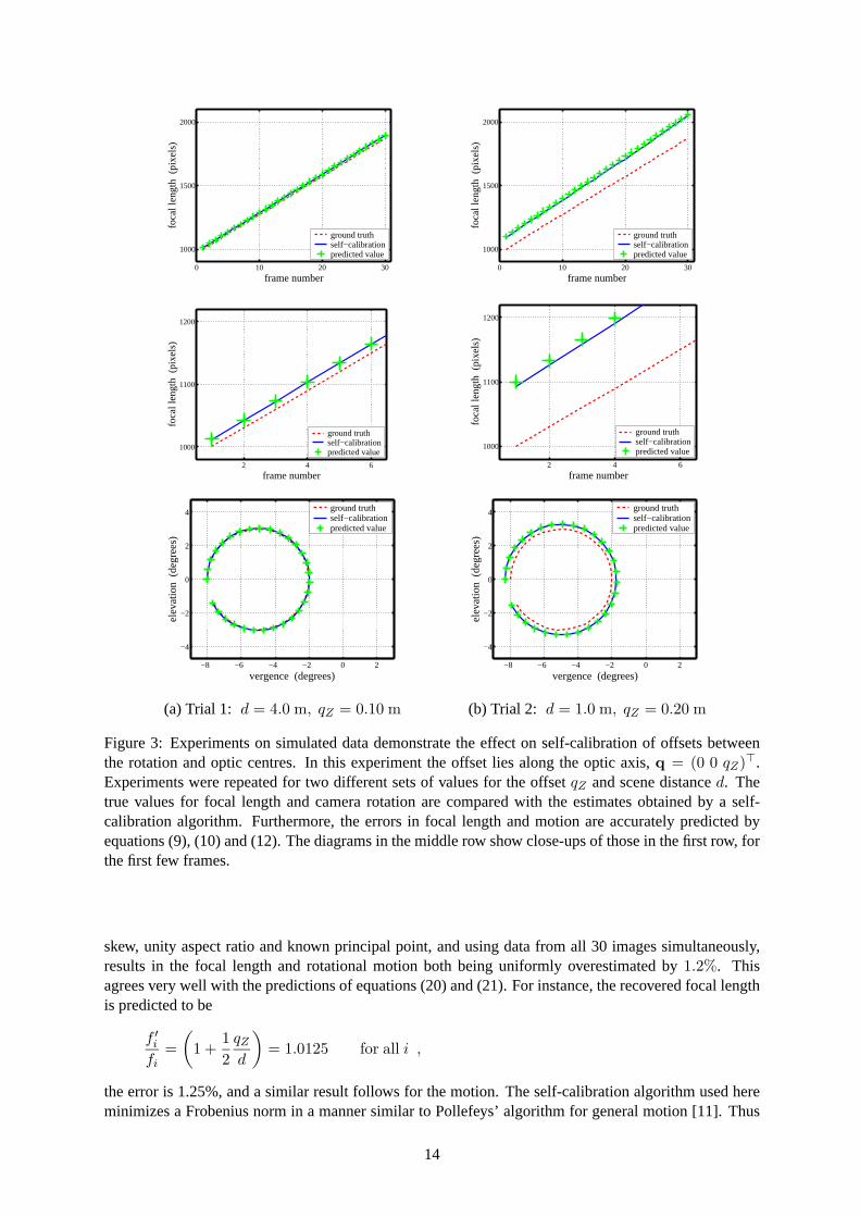
Figure 3: Experiments on simulated data demonstrate the effect on self-calibration of offsets betweenthe rotation and optic centres. In this experiment the offset lies along the optic axis, q = (0 0 qZ).Experiments were repeated for two different sets of values for the offset qZ and scene distance d. Thetrue values for focal length and camera rotation are compared with the estimates obtained by a self-calibration algorithm. Furthermore, the errors in focal length and motion are accurately predicted byequations (9), (10) and (12). The diagrams in the middle row show close-ups of those in the first row, forthe first few frames.
skew, unity aspect ratio and known principal point, and using data from all 30 images simultaneously,results in the focal length and rotational motion both being uniformly overestimated by 1.2%. Thisagrees very well with the predictions of equations (20) and (21). For instance, the recovered focal lengthis predicted to be
f ′i
fi=
(1 +
12
qZ
d
)= 1.0125 for all i ,
the error is 1.25%, and a similar result follows for the motion. The self-calibration algorithm used hereminimizes a Frobenius norm in a manner similar to Pollefeys’ algorithm for general motion [11]. Thus
14
it obtains estimates of focal length in quite a different manner from the technique used in Section 3 topredict the recovered focal lengths. This adds weight to the argument that the predicted errors in thispaper are largely independent of the choice of self-calibration algorithm and that the expressions wederived hold regardless of the number of images used by the self-algorithm program.
In the second trial d = 1.0 m and qZ = 0.20 m so that the ratio qZ/d is considerably larger than before.The plots of focal length and motion recovered by assuming pure rotation in Figure 3b show errors of9.3% whereas the predictions of equations (20) and (21) are 10.0%. In fact, the discrepancy is causedlargely by the binomial expansion of the square root in these equations. Avoiding this approximationyields
f ′i
fi=
√1 +
qZ
d= 1.095 for all i ,
that is a 9.5% error obtained by our predictions compared with a 9.3% error from experiments.
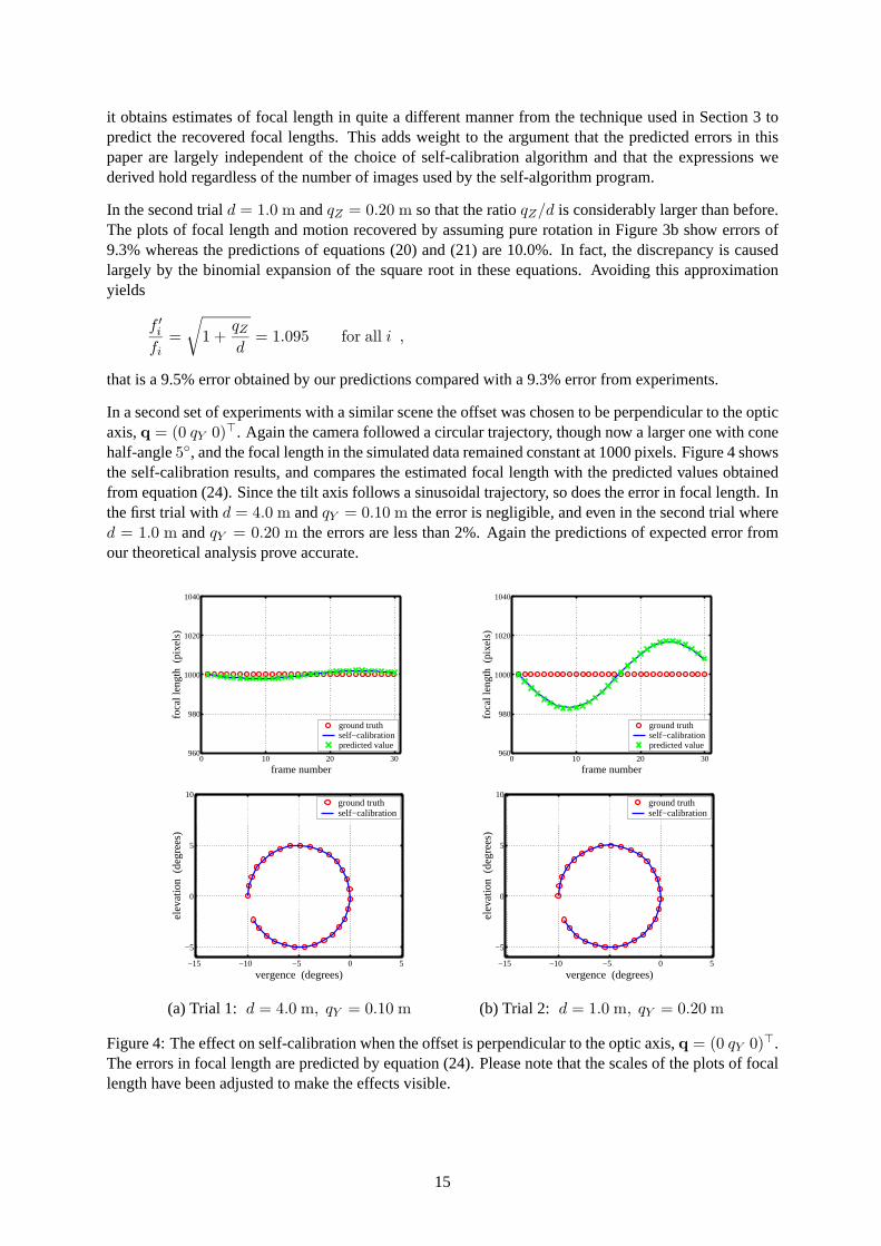
In a second set of experiments with a similar scene the offset was chosen to be perpendicular to the opticaxis, q = (0 qY 0). Again the camera followed a circular trajectory, though now a larger one with conehalf-angle 5, and the focal length in the simulated data remained constant at 1000 pixels. Figure 4 showsthe self-calibration results, and compares the estimated focal length with the predicted values obtainedfrom equation (24). Since the tilt axis follows a sinusoidal trajectory, so does the error in focal length. Inthe first trial with d = 4.0 m and qY = 0.10 m the error is negligible, and even in the second trial whered = 1.0 m and qY = 0.20 m the errors are less than 2%. Again the predictions of expected error fromour theoretical analysis prove accurate.
0 10 20 30960
980
1000
1020
1040
frame number
foca
l len
gth
(pi
xels
)
ground truth self−calibrationpredicted value
0 10 20 30960
980
1000
1020
1040
frame number
foca
l len
gth
(pi
xels
)
ground truth self−calibrationpredicted value
−15 −10 −5 0 5
−5
0
5
10
vergence (degrees)
elev
atio
n (
degr
ees)
ground truth self−calibration
−15 −10 −5 0 5
−5
0
5
10
vergence (degrees)
elev
atio
n (
degr
ees)
ground truth self−calibration
(a) Trial 1: d = 4.0 m, qY = 0.10 m (b) Trial 2: d = 1.0 m, qY = 0.20 m
Figure 4: The effect on self-calibration when the offset is perpendicular to the optic axis, q = (0 qY 0).The errors in focal length are predicted by equation (24). Please note that the scales of the plots of focallength have been adjusted to make the effects visible.
15
6 Discussion
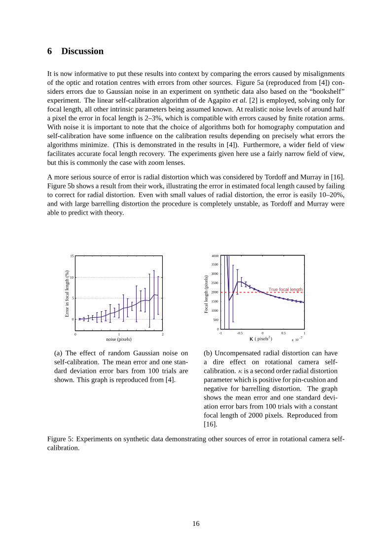
It is now informative to put these results into context by comparing the errors caused by misalignmentsof the optic and rotation centres with errors from other sources. Figure 5a (reproduced from [4]) con-siders errors due to Gaussian noise in an experiment on synthetic data also based on the “bookshelf”experiment. The linear self-calibration algorithm of de Agapito et al. [2] is employed, solving only forfocal length, all other intrinsic parameters being assumed known. At realistic noise levels of around halfa pixel the error in focal length is 2–3%, which is compatible with errors caused by finite rotation arms.With noise it is important to note that the choice of algorithms both for homography computation andself-calibration have some influence on the calibration results depending on precisely what errors thealgorithms minimize. (This is demonstrated in the results in [4]). Furthermore, a wider field of viewfacilitates accurate focal length recovery. The experiments given here use a fairly narrow field of view,but this is commonly the case with zoom lenses.
A more serious source of error is radial distortion which was considered by Tordoff and Murray in [16].Figure 5b shows a result from their work, illustrating the error in estimated focal length caused by failingto correct for radial distortion. Even with small values of radial distortion, the error is easily 10–20%,and with large barrelling distortion the procedure is completely unstable, as Tordoff and Murray wereable to predict with theory.
0 1 2
noise (pixels)
Err
or in
foc
al le
ngth
(%
)
0
5
10
15
-1 -0.5 0 0.5 1
10-7
0
500
1000
1500
2000
2500
3000
3500
4000
True focal length
κ ( pixels )2
Foca
l len
gth
(pix
els)
x
(a) The effect of random Gaussian noise onself-calibration. The mean error and one stan-dard deviation error bars from 100 trials areshown. This graph is reproduced from [4].
(b) Uncompensated radial distortion can havea dire effect on rotational camera self-calibration. κ is a second order radial distortionparameter which is positive for pin-cushion andnegative for barrelling distortion. The graphshows the mean error and one standard devi-ation error bars from 100 trials with a constantfocal length of 2000 pixels. Reproduced from[16].
Figure 5: Experiments on synthetic data demonstrating other sources of error in rotational camera self-calibration.
16
7 Closed loop constraints
Information supplementary to the infinite homography constraint in equation (2) is available from knowl-edge that the camera returned to its initial orientation. Kang and Weiss [10] used this notion when solvingfor a constant focal length from full 360 panoramic mosaics. However, in the absence of noise, and forthe cases considered in this paper, these “closed loop” constraints are satisfied automatically and thushave no influence on the solution. We demonstrate this for Cases 1, 2 and 3 before discussing whenclosed loop constraints are useful even in the absence of noise.
The key point is that in both Case 1 and Case 2, if the camera returns to its point of origin, and the sameeffective scene plane has been viewed throughout the entire sequence, R = I, t = 0 and the homographyis of the form
H0i = KiK−10 =
fi
f00 0
0 fi
f00
0 0 1
, (28)
and inserting estimates of focal lengths into matrices K′0 and K′i of intrinsic parameters gives the recoveredrotation matrix
R′ = K′i−1HK′0 = K′i
−1KiK
−10 K′0.
Now, let us assume that the focal length in the reference frame is incorrectly estimated, f ′0 = f0. Re-
gardless, the infinite homography constraint for frame i is satisfied perfectly if f ′i = (fi/f0)f ′
0. Therecovered rotation is then found as
R′ = K′i−1KiK
−10 K′0 = I.
In other words, the rotation in frame i is recovered correctly, regardless of whether the closed loopconstraint is applied or not. The closed loop constraint is satisfied automatically and does not provideany further information. This analysis holds independent of whether a small angle approximation is usedor not, and is also independent of the orientation of the effective scene plane.
The closed loop constraint does not provide further information in Case 3 either. Here a translation alongthe optic axis towards a fronto-parallel plane is compensated by an erroneous change in focal length.Again R′ = I and θ′ = 0. However, this result no longer holds when the plane is not fronto-parallel.
Closed loop constraints are useful when extending the analysis to multiple effective scene planes; whengenerating a mosaic from a wide range of orientations of the camera, the assumption of a single effectivescene plane (which is not at infinity) is unreasonable given the limited field of view of cameras. In realitythere will be a set of effective scene planes around the camera, these planes being more or less fronto-parallel when they are visible. If a homography H0,i is computed as a concatenation of homographies,
H0,i = Hi−1,iHi−2,i−1...H0,1 ,
as the camera returns to the original position this homography will in general not be diagonal due to thedifferent scene planes. For instance, assume a three frame sequence 0, 1, 2 where the camera positionand orientation are identical in the first and last frames. One may verify that concatenating homographiesas H0,2 = H2,1H1,0 gives a diagonal matrix only if the scene planes viewed between frames 0, 1 and1, 2 are the same. Knowing that the camera has returned to its starting point thus places a constraint thatthis homography must be diagonal, and this will in turn have an effect on the self-calibration results. Thisconstraint can, in fact, be applied directly to the homographies in a bundle-adjustment in the homographyparameters and points on a planar mosaic. Only a single parameter need be included in a frame knownto have the same orientation as the starting position. This parameter takes care of an unknown zoom and
17
corresponds to fi/f0 in equation (28). For a full panoramic mosaic this information may alternativelybe used in a Euclidean space in the manner of Kang and Weiss [10] by iteratively recomputing thefocal lengths and compositing length of the mosaic (the length of the panoramic image) such that thecompositing length (hopefully) approaches the veridical value. However, it turns out that this schemecould diverge with finite rotation arms, as will be seen in Section 9.
Finally, we briefly mention what happens if translations are caused by shaky operation of a hand-heldcamera giving rise to translations in the x, y−plane, say t = (0 tY 0), which are not coupled to therotation angle θ. This scenario has not been considered otherwise in this paper, and is more akin to thatconsidered by Wang et al. [19] who show that errors in focal length are then larger for small rotations. Inthis case the camera may return to its original orientation, but because of translations, the homography isno longer diagonal, and the infinite homography constraint is not satisfied. Force-fitting an orthonormalmatrix to K′i
−1HK′0 does not give θ = 0. Therefore, applying a closed loop constraint would certainlyaffect the solution, although we have not investigated what this effect would be.
8 Constraints independent of translations
For constant focal length and planes which are fronto-parallel to the initial frame, Wang et al. [19]derived closed-form solutions for the focal length independent of translations. We now demonstrate thatthese equations give insufficient constraints with varying focal length, and moreover that they are weakconstraints, both because of sensitivity to noise, and because the results are heavily reliant on the planeactually being fronto-parallel with respect to the first frame. We will see that these equations tend to themeaningless 0 = 0 for first order approximations of rotation angles. Either side of the equation onlybecomes non-zero due to noise, translations of the camera, or second order terms in the sin and cos ofrotation angles. Therefore, if used in combination with all other available equations from the infinitehomography constraint in equation (2), they will fail to influence the solution for small rotations. Theygive solutions which cannot explain the observed image motion in Section 4.
In adapting the constraints of Wang et al. [19] to varying intrinsics, the homography must first be givenfor a general rotation matrix, and with n = (0 0 1)
H01 = K1
(R +
1dtn
)K−1
0 =
f1
f0r11
f1
f0r12 f1(r13 + tX
d )f1
f0r21
f1
f0r22 f1(r23 + tY
d )1f0
r311f0
r32 (r33 + tZd )
=
r11 r12 f0(r13 + tX
d )r21 r22 f0(r23 + tY
d )1f1
r311f1
r32f0
f1(r33 + tZ
d )
.
Considering the first two columns of this matrix, constraints which are independent of the translation areobtained by requiring the first two columns of the rotation matrix R to be of equal length and orthogonal.The constraints are
h211 + h2
21 + f ′12h2
31 = h212 + h2
22 + f ′12h2
32 (29)
⇒ f ′12 =
h211 + h2
21 − h212 − h2
22
h232 − h2
31
(30)
18
provided h232 − h2
31 = 0, and
h11h12 + h21h22 + f ′12h31h32 = 0 (31)
⇒ f ′12 = −h11h12 + h21h22
h31h32(32)
provided h31h32 = 0. It should be noted that the second equation may not be used if the rotation is apure pan or pure tilt since then either h31 or h32 is zero.
From these equations we see that although f1 may be recovered in this manner, there are no constraintson f0. Thus the fact that we have varying intrinsics invalidates this approach. Including further imagesin a self-calibration algorithm based on these constraints does not help solve for f0 either.
To be more precise, we are unable to obtain information concerning the focal length in any frame inwhich the optic axis is perpendicular to the plane in the scene, i.e. when R is the identity or a rotationsolely about z. In theory, if one knows a priori the orientation of the plane with respect to one ormore of the images, then referring all homographies to a reference frame with that orientation meansthat the focal length may be recovered for all frames not at that orientation. If no frames have thisdegenerate orientation, all focal lengths could be recovered. However, such an assumption is based onprior Euclidean knowledge concerning angles.
If these constraints are degenerate for orientations of the camera perpendicular to the plane, it seemslikely that they are near-degenerate for orientations of the camera close to perpendicular to the plane. Afirst order approximation to the rotation matrix is
R ≈ 1 −θz θy
θz 1 −θx
−θy θx 1
.
where θx, θy and θz are the rotations about the x, y and z axes respectively. One may readily verify thatwith this approximation of R, equation (29) reduces to 0 = 0 while (31) becomes θxθyf1 = θxθyf
′1 and
thus relies on second order terms to compute the focal length. We will shortly demonstrate that whentaking second order approximations, the correct solution is found for f1 also from equation (29) providedthe plane really is fronto-parallel. Since these equations rely on second order terms they are extremelysensitive to noise for small rotations, but could function well for frames whose orientations are far fromthe reference frame. With other constraints a first order approximation is sufficient to correctly determinethe focal lengths; for instance substitute q = 0 in equations (9) to (12).
With misalignments the question arises of how important the assumption of a fronto-parallel plane is forrecovering the focal length in this manner. Therefore we investigate what happens if this is not the case,n = (nX nY nZ). For this we shall assume q = (0 0 qZ) and pure tilt, and we use a second orderapproximation to the rotation matrix such that
t = Rq − q =
0
−θqZ
− θ2
2 qZ
.
and
H =
1 0 0
− qZd θnX 1 − θ2
2 − qZd θnY −f0θ
(1 + qZ
d nZ
)− 1
f1
qZd
θ2
2 nX1f1
θ f0
f1
(1 − θ2
2 − qZd
θ2
2 nZ
)
.
19
Using equation (30) to compute f ′1 gives
f ′12 =
h211 + h2
21 − h212 − h2
22
h232 − h2
31
= f21
1 + ( qZd θnX)2 − (1 − θ2
2 − qZd θnY )2
θ2 −(
qZd
θ2
2 nX
)2
≈ f21
1 + ( qZd θnX)2 − (1 − θ2 − 2 qZ
d θnY )θ2
≈ f21
(1 + 2
qZ
d
nY
θ
)f ′1 ≈ f1
√1 + 2
qZ
d
nY
θ≈ f1
(1 +
qZ
d
nY
θ
). (33)
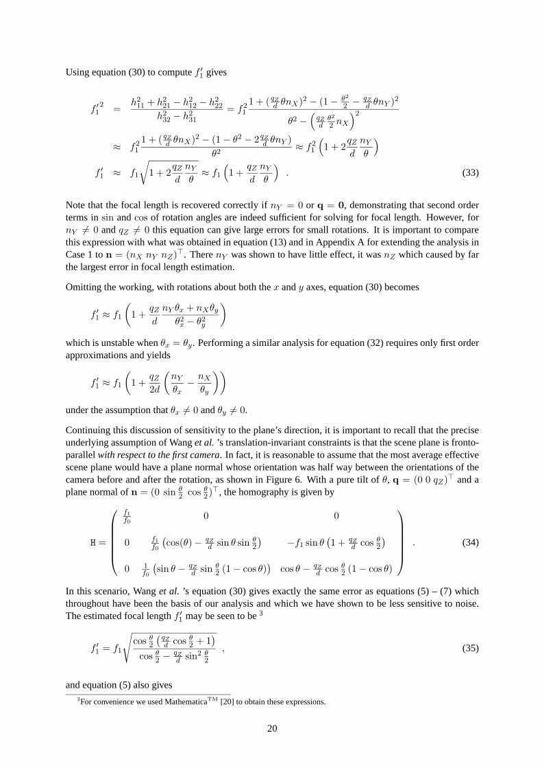
Note that the focal length is recovered correctly if nY = 0 or q = 0, demonstrating that second orderterms in sin and cos of rotation angles are indeed sufficient for solving for focal length. However, fornY = 0 and qZ = 0 this equation can give large errors for small rotations. It is important to comparethis expression with what was obtained in equation (13) and in Appendix A for extending the analysis inCase 1 to n = (nX nY nZ). There nY was shown to have little effect, it was nZ which caused by farthe largest error in focal length estimation.
Omitting the working, with rotations about both the x and y axes, equation (30) becomes
f ′1 ≈ f1
(1 +
qZ
d
nY θx + nXθy
θ2x − θ2
y
)
which is unstable when θx = θy. Performing a similar analysis for equation (32) requires only first orderapproximations and yields
f ′1 ≈ f1
(1 +
qZ
2d
(nY
θx− nX
θy
))
under the assumption that θx = 0 and θy = 0.
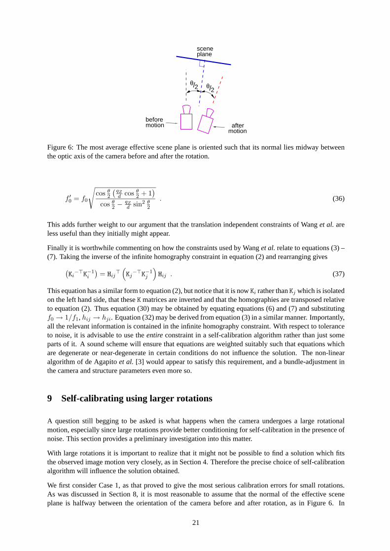
Continuing this discussion of sensitivity to the plane’s direction, it is important to recall that the preciseunderlying assumption of Wang et al. ’s translation-invariant constraints is that the scene plane is fronto-parallel with respect to the first camera. In fact, it is reasonable to assume that the most average effectivescene plane would have a plane normal whose orientation was half way between the orientations of thecamera before and after the rotation, as shown in Figure 6. With a pure tilt of θ, q = (0 0 qZ) and aplane normal of n = (0 sin θ
2 cos θ2), the homography is given by
H =
f1
f00 0
0 f1
f0
(cos(θ) − qZ
d sin θ sin θ2
) −f1 sin θ(1 + qZ
d cos θ2
)0 1
f0
(sin θ − qZ
d sin θ2 (1 − cos θ)
)cos θ − qZ
d cos θ2 (1 − cos θ)
. (34)
In this scenario, Wang et al. ’s equation (30) gives exactly the same error as equations (5) – (7) whichthroughout have been the basis of our analysis and which we have shown to be less sensitive to noise.The estimated focal length f ′
1 may be seen to be 3
f ′1 = f1
√cos θ
2
( qZd cos θ
2 + 1)
cos θ2 − qZ
d sin2 θ2
, (35)
and equation (5) also gives3For convenience we used MathematicaTM [20] to obtain these expressions.
20
scene
aftermotion before
θ
plane
motion
2/ θ 2/
Figure 6: The most average effective scene plane is oriented such that its normal lies midway betweenthe optic axis of the camera before and after the rotation.
f ′0 = f0
√cos θ
2
( qZd cos θ
2 + 1)
cos θ2 − qZ
d sin2 θ2
. (36)
This adds further weight to our argument that the translation independent constraints of Wang et al. areless useful than they initially might appear.
Finally it is worthwhile commenting on how the constraints used by Wang et al. relate to equations (3) –(7). Taking the inverse of the infinite homography constraint in equation (2) and rearranging gives
(Ki
−K−1i
)= Hij
(Kj
−K−1j
)Hij . (37)
This equation has a similar form to equation (2), but notice that it is now Ki rather than Kj which is isolatedon the left hand side, that these K matrices are inverted and that the homographies are transposed relativeto equation (2). Thus equation (30) may be obtained by equating equations (6) and (7) and substitutingf0 → 1/f1, hij → hji. Equation (32) may be derived from equation (3) in a similar manner. Importantly,all the relevant information is contained in the infinite homography constraint. With respect to toleranceto noise, it is advisable to use the entire constraint in a self-calibration algorithm rather than just someparts of it. A sound scheme will ensure that equations are weighted suitably such that equations whichare degenerate or near-degenerate in certain conditions do not influence the solution. The non-linearalgorithm of de Agapito et al. [3] would appear to satisfy this requirement, and a bundle-adjustment inthe camera and structure parameters even more so.
9 Self-calibrating using larger rotations
A question still begging to be asked is what happens when the camera undergoes a large rotationalmotion, especially since large rotations provide better conditioning for self-calibration in the presence ofnoise. This section provides a preliminary investigation into this matter.
With large rotations it is important to realize that it might not be possible to find a solution which fitsthe observed image motion very closely, as in Section 4. Therefore the precise choice of self-calibrationalgorithm will influence the solution obtained.
We first consider Case 1, as that proved to give the most serious calibration errors for small rotations.As was discussed in Section 8, it is most reasonable to assume that the normal of the effective sceneplane is halfway between the orientation of the camera before and after rotation, as in Figure 6. In
21
0 45 90 135 1800
0.5
1
1.5
2
Rotation angle θ (degrees)
Rec
over
ed r
elat
ive
foca
l len
gth,
f ′ / f All equations
0 45 90 135 1800
0.5
1
1.5
2
Rotation angle θ (degrees)
Rec
over
ed r
elat
ive
foca
l len
gth,
f ′ / f Equation (5)
Equation (6)Equation (7)
(a) The relative focal length recovered fromtwo images when the effective scene plane isoriented as in Figure 6, i.e. midway betweenthe camera configurations before and after ro-tation. The equations give consistent results,and are stable for a large range of camera rota-tions.
(b) The relative focal length recovered fromtwo images from various equations under theassumption that the effective scene plane isfronto-parallel with respect to the first frame
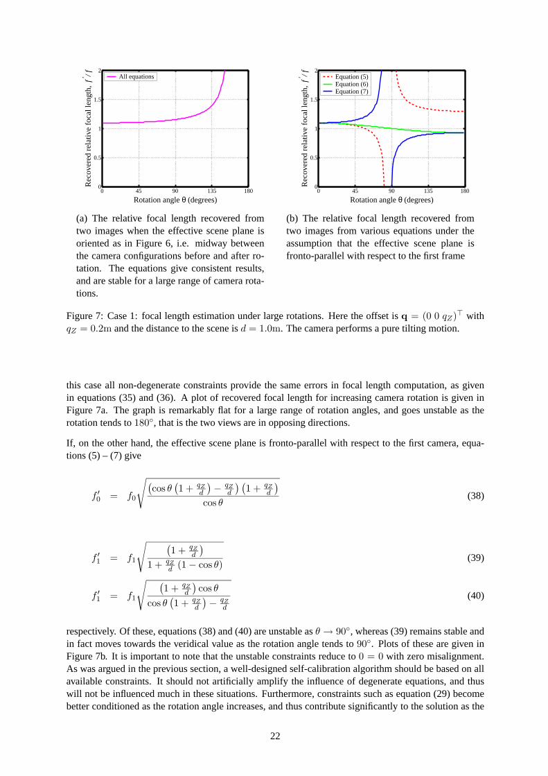
Figure 7: Case 1: focal length estimation under large rotations. Here the offset is q = (0 0 qZ) withqZ = 0.2m and the distance to the scene is d = 1.0m. The camera performs a pure tilting motion.
this case all non-degenerate constraints provide the same errors in focal length computation, as givenin equations (35) and (36). A plot of recovered focal length for increasing camera rotation is given inFigure 7a. The graph is remarkably flat for a large range of rotation angles, and goes unstable as therotation tends to 180, that is the two views are in opposing directions.
If, on the other hand, the effective scene plane is fronto-parallel with respect to the first camera, equa-tions (5) – (7) give
f ′0 = f0
√(cos θ
(1 + qZ
d
) − qZd
) (1 + qZ
d
)cos θ
(38)
f ′1 = f1
√ (1 + qZ
d
)1 + qZ
d (1 − cos θ)(39)
f ′1 = f1
√ (1 + qZ
d
)cos θ
cos θ(1 + qZ
d
) − qZd
(40)
respectively. Of these, equations (38) and (40) are unstable as θ → 90, whereas (39) remains stable andin fact moves towards the veridical value as the rotation angle tends to 90. Plots of these are given inFigure 7b. It is important to note that the unstable constraints reduce to 0 = 0 with zero misalignment.As was argued in the previous section, a well-designed self-calibration algorithm should be based on allavailable constraints. It should not artificially amplify the influence of degenerate equations, and thuswill not be influenced much in these situations. Furthermore, constraints such as equation (29) becomebetter conditioned as the rotation angle increases, and thus contribute significantly to the solution as the
22
camera rotation increases. Therefore, in practice it is possible to recover f0, albeit with some error, evenwhen the rotation is exactly 90 in this scenario. For instance, with rather extreme values of qZ = 0.2 mand d = 1.0 m, the non-linear algorithm of de Agapito et al. [3] gave f ′
0 = 1.201f0 and f ′1 = 0.986f1.
The translation in this experiment is very significant, the errors are still of the order qZ/d. It is interestingto note, however, that when the translation of the camera is directly coupled to its rotation, as here, largerrotations do not provide more accurate focal length recovery. We also attempted the linear algorithm ofde Agapito et al. [2] on this data and got significantly worse results.
In practice, a common procedure is to self-calibrate from a sequence of images where neighbouringimages have significant overlap, but the aggregate rotation is large. A set of homographies, all referredto a common reference frame can be obtained by concatenating homographies from image pairs
H0,i = Hi−1,iHi−2,i−1...H0,1 .
We investigate what errors in focal length recovery will be encountered in this scenario, assuming that (i)the translational misalignment is that of Case 1, (ii) that successive rotations are by an equal amount, (iii)that the distance to the effective scene plane is the same for all image pairs, and finally (iv) that for eachimage pair, the normal of the effective scene plane is located midway between the orientations of eachimage pair as in Figure 6 (note that this does not mean that the effective scene plane is the same over theentire sequence). This albeit strong set of assumptions leads to a somewhat curious result4: the recoveredfocal length is still given by equation (35) though now for any frame i. If the individual rotations aresmall, the error in focal length is therefore accurately predicted by the rotation-invariant equations (9)and (10) from Section 3. Admittedly, this result no longer holds when the rotations between image pairsdiffer, when the distance to the scene varies, and when the orientation of the scene plane varies, but wehave found empirically in unreported experiments that in many cases it at least provides an approximateupper bound on the error. In summary, the expressions derived right at the begin of this paper for Case1 provide useful insight even with large composite rotations if knowledge of the minimum or averageeffective scene depth is available.
With equidistant and fronto-parallel effective scene planes, and equal, small rotations between pairs ofviews, the rotations are of course recovered as θ ′
i ≈ θi( 1 + qZ/(2d) ). Consider the camera performinga full 360 turn while creating a panoramic mosaic, and assume that it is known that the camera returnsto its initial position. From equation (12) the recovered rotation at the end of the panorama would be
θ′ ≈ 2π(1 +
qZ
2d
)where θi is the constant rotation between pairs of images. This rotation does not agree with the priorknowledge. Hence, multiplying the estimates of focal length by 2π/θ′ would in fact virtually remove theerror in focal length estimation! Sadly, in pratice this result does not hold since it is usually not possibleto justify the assumption of equidistant effective scene planes over such a large rotation. Furthermore,although the magnitude of the misalignment vector q need not be known in advance in this strategy,its direction must be. Moreover, adjusting the self-calibration in this manner could be dangerous in thepresence of noise or uncorrected radial distortion.
Note also that this way of adjusting the focal length estimate is quite different to the method proposedby Kang and Weiss [10]. In their method, overestimating the total rotation (and hence the compositelength defined as L′ = θ′f ′) indicates that the focal length has been underestimated, and they advocatean iterative scheme to improve the solution. Assuming constant intrinsic parameters and starting withthe initial solution from equation (9)
f ′ ≈ f(1 +
qZ
2d
)4We verified this using MathematicaTM [20].
23
the first step involves recomputing the focal length as
f ′ ← L′
2π= f
(1 +
qZ
d
)The focal lengths are in fact multplied by the inverse of the appropriate corrective factor, and the error infocal length therefore squares! Subsequently, the estimated composite length increases further, and thescheme diverges. Disturbingly, an algorithm which was good at battling noise is unstable with this formof misalignment.
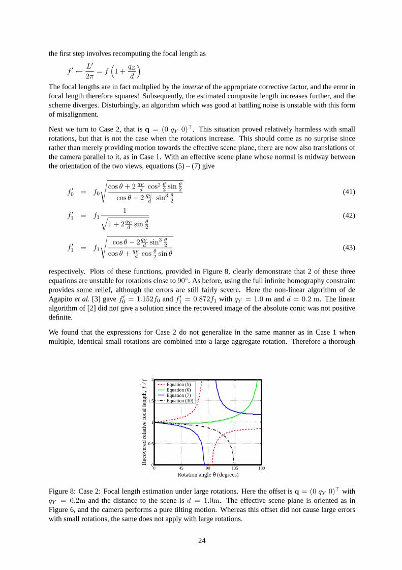
Next we turn to Case 2, that is q = (0 qY 0). This situation proved relatively harmless with smallrotations, but that is not the case when the rotations increase. This should come as no surprise sincerather than merely providing motion towards the effective scene plane, there are now also translations ofthe camera parallel to it, as in Case 1. With an effective scene plane whose normal is midway betweenthe orientation of the two views, equations (5) – (7) give
f ′0 = f0
√cos θ + 2 qY
d cos2 θ2 sin θ
2
cos θ − 2 qYd sin3 θ
2
(41)
f ′1 = f1
1√1 + 2 qY
d sin θ2
(42)
f ′1 = f1
√cos θ − 2 qY
d sin3 θ2
cos θ + qYd cos θ
2 sin θ(43)
respectively. Plots of these functions, provided in Figure 8, clearly demonstrate that 2 of these threeequations are unstable for rotations close to 90. As before, using the full infinite homography constraintprovides some relief, although the errors are still fairly severe. Here the non-linear algorithm of deAgapito et al. [3] gave f ′
0 = 1.152f0 and f ′1 = 0.872f1 with qY = 1.0 m and d = 0.2 m. The linear
algorithm of [2] did not give a solution since the recovered image of the absolute conic was not positivedefinite.
We found that the expressions for Case 2 do not generalize in the same manner as in Case 1 whenmultiple, identical small rotations are combined into a large aggregate rotation. Therefore a thorough
0 45 90 135 1800
0.5
1
1.5
2
Rotation angle θ (degrees)
Rec
over
ed r
elat
ive
foca
l len
gth,
f ′ / f Equation (5)
Equation (6)Equation (7)Equation (30)
Figure 8: Case 2: Focal length estimation under large rotations. Here the offset is q = (0 qY 0) withqY = 0.2m and the distance to the scene is d = 1.0m. The effective scene plane is oriented as inFigure 6, and the camera performs a pure tilting motion. Whereas this offset did not cause large errorswith small rotations, the same does not apply with large rotations.
24
empirical investigation is required, also into whether knowledge of full 360 rotations proves beneficial,although this falls beyond the scope of this paper.
State-of-the-art self-calibration software should incorporate one or more bundle-adjustment stages [18].Initially, the set of homographies can be bundle-adjusted in a projective space to reduce sensitivity toaccumulated errors caused by concatenating homographies. This will in effect select a single effectivescene plane over the entire sequence. It is not obvious what the new, overall effective scene plane will bewhen the total rotation is very large, and consequently the effects of such a procedure on the recovery ofcamera intrinsic parameters are unclear, it is possible that the bundle-adjustment would “push” the singleeffective scene plane further away from the camera, leading to more accurate focal length estimation. Weleave this as a topic for future research. Finally, one can also bundle-adjust in the Euclidean extrinsic,intrinsic and structure parameters. In this stage it would also be possible to explicitly model knownor unknown misalignments with a limited number of parameters, although there is always a dangerassociated with adding extra unknowns in the presence of noise; we are faced with a model-selectionproblem.
In summary, when the length of the rotation arm is constant, in the absence of noise, and when usingconcatenated homographies to self-calibrate, there seems no advantage associated with self-calibratingfrom large rather than small rotations. To provide a rough rule of thumb, the maximum relative errorin focal length estimation one is likely to encounter with large rotations is about |q|/dmin where dmin
is the minimum distance to the scene, although further experimentation is certainly required to supportthis claim. However, some relief might be available by performing a bundle-adjustment or incorporatingknowledge that the camera has returned to its original orientation.
10 Conclusions
In this paper we have developed expressions describing the errors introduced when the assumption of apure rotation about the camera’s optic centre is violated. The key results in this paper are independentof the particular self-calibration algorithm up to a first order approximation of rotations, provided theimages are noiseless. These conclusions are primarily arrived at for cases when the rotation arm is offixed length, as is indeed the case with many cameras mounted on tripods or robotic heads. Moreover,this paper only considers the case when the focal length is the sole unknown parameter, although this ispermitted to vary from image to image. The results clearly show that the assumption of a pure rotationis a perfectly good one in many practical situations when the distance to the scene is large in comparisonwith the translations of the camera. This is a relief since techniques for self-calibration from sequenceswithout translation have considerable practical advantages over the equivalent algorithms for generalmotion: robust feature matching is vastly simplified since the mapping between image pairs is one-to-one rather than one-to-many, and the plane at infinity need not be estimated.
A very brief discussion was provided for errors likely to be encountered when the camera undergoesa much larger rotation. However, this topic merits further research in the form of extensive empiri-cal evaluation of different self-calibration algorithms. Larger rotations are in general beneficial for theconditioning of the self-calibration problem, especially when solving for other intrinsic parameters thanjust focal length. Thus with large rotations it would also be meaningful to consider how translationalmisalignments affect the recovery of the aspect ratio, skew and principal point.
25
Appendix A
This Appendix demonstrates that the assumption of a fronto-parallel plane is not critical when de-riving the results of Case 1 in Section 3. Thus we permit the plane normal to take a general formn = (nX nY nZ). As before we assume pure tilt, and use a third order approximation to the rotationmatrix such that
t = Rq − q =
0
−(θ − θ3
6 )qZ
− θ2
2 qZ
. (44)
Systematically ignoring fourth order and higher terms gives the homography
H =
f1
f00 0
−f1
f0
qZd θnX
f1
f0
(1 − θ2
2 − qZd θnY
)−f1θ
(1 − θ2
6 + qZd nZ
)
− 1f0
qZd
θ2
2 nX1f0
θ(1 − θ2
6 − qZd nY
θ2
) (1 − θ2
2 − qZd
θ2
2 nZ
)
.
Computing f0 from equation (5) gives
f ′02 = −
−f1θ(1 − θ2
6 + qZd nZ
) (1 − θ2
2 − qZd
θ2
2 nZ
)f1
f20θ(1 − θ2
2 − qZd θnY
) (1 − θ2
6 − qZd nY
θ2
)
= f20
1 − 2θ2
3 + qZd nZ − qZ
dθ2
2 nZ
1 − 2θ2
3 − qZd
3θ2 nY
= f20
(1 − 2θ2
3+
qZ
dnZ − qZ
d
θ2
2nZ
) (1 +
2θ2
3+
qZ
d
3θ
2nY
)
= f20
(1 +
qZ
dnZ +
qZ
d
3θ
2nY
)+ O(3)
f ′0 = f0
(1 +
qZ
2dnZ +
qZ
d
3θ
4nY
)+ O(3) . (45)
The additional error caused by nY is a second order term since qZ/d and θ are small. In fact, if nY 1,i.e. the effective scene plane is roughly fronto-parallel, then this additional error is a third order term.
Similarly, equation (6) may be used to find f1. Ignoring third order terms where it is safe to do so yields5
f ′12 =
f20
(1 + qZ
d nZ + qZd
3θ2 nY
) (f1
f0
)2
f20
(1 + qZ
d nZ + qZd
3θ2 nY
)1f20θ2 +
(1 − θ2
2 − qZd
θ2
2 nZ
)2 + O(3)
= f21
1 + qZd nZ + qZ
d3θ2 nY
θ2 + qZd θ2nZ + 1 − θ2
+ O(3)
= f21
(1 +
qZ
dnZ +
qZ
d
3θ
2nY
)+ O(3)
f ′1 = f1
(1 +
qZ
2dnZ +
qZ
d
3θ
4nY
)+ O(3) . (46)
5Whenever a term appears as 1 +O(3), and the 1 does not get cancelled by subtracting by 1, we may ignore the third orderterm. However, third order terms must be considered in expressions such as θ + θ2 qZ
d= θ(1 + θ qZ
d) since the common factor
of θ may (and does) cancel out, giving a term 1 + O(2).
26
Using equation (7) to compute f ′1 gives a slightly different answer. Since the denominator is the same in
equations (6) and (7), and because we ignore third order terms, the denominator is simply 1.
f ′12 = f2
0
(1 +
qZ
dnZ +
qZ
d
3θ
2nY
) (f1
f0
)2 (1 − θ2
2− qZ
dθnY
)2
+f21 θ2
(1 − θ2
6+
qZ
dnZ
)2
+ O(3)
= f21
((1 +
qZ
dnZ +
qZ
d
3θ
2nY
) (1 − θ2 − 2θ
qZ
dnY
)+ θ2
)+ O(3)
= f21
(1 +
qZ
dnZ − θ
qZ
2dnY
)+ O(3)
f ′1 = f1
(1 +
qZ
2dnZ − qZ
d
θ
4nY
)+ O(3) . (47)
In both expressions for f ′1 the dependency on nY is again second order, or third order if nY 1.
In conclusion, the expressions provided for Case 1 in Section 3 are unaffected by the plane being slightlyoff fronto-parallel.
References
[1] J.R. Bergen, P. Anandan, K.J. Hanna, and R. Hingorani. Hierarchical model-based motion esti-mation. In Proc. 2nd European Conference on Computer Vision, Santa Margharita Ligure, Italy,pages 237–252, 1992.
[2] L. de Agapito, R. I. Hartley, and E. Hayman. Linear calibration of a rotating and zooming camera.In Proc. IEEE Conference on Computer Vision and Pattern Recognition, Fort Collins, Colorado,pages I: 15–21, 1999.
[3] L. de Agapito, E. Hayman, and I. Reid. Self-calibration of a rotating camera with varying intrinsicparameters. In Proc. 9th British Machine Vision Conference, Southampton, pages 105–114, 1998.
[4] L. de Agapito, E. Hayman, and I. Reid. Self-calibration of rotating and zooming cameras. Interna-tional Journal of Computer Vision, 45(2):107–127, 2001.
[5] M.A. Fischler and R.C. Bolles. Random sample concensus: A paradigm for model fitting withapplications to image analysis and automated cartography. Comm. ACM, 24(6):381–395, 1981.
[6] R. I. Hartley. Self-calibration of stationary cameras. International Journal of Computer Vision,22(1):5–23, February 1997.
[7] R. I. Hartley and A. Zisserman. Multiple View Geometry in Computer Vision. Cambridge UniversityPress, ISBN: 0521623049, 2000.
[8] E. Hayman. The Use of Zoom within Active Vision. PhD thesis, Department of Engineering Science,University of Oxford, 2000.
[9] E. Hayman, L. de Agapito, I. D. Reid, and D. W. Murray. The role of self-calibration in Euclideanreconstruction from two rotating and zooming cameras. In Proc. 6th European Conference onComputer Vision, Dublin, Ireland, pages II: 477–492, 2000.
[10] S.B. Kang and R. Weiss. Characterization of errors in compositing panoramic images. ComputerVision and Image Understanding, 73(2):269–280, February 1999.
[11] M. Pollefeys, R. Koch, and L. Van Gool. Self calibration and metric reconstruction in spite ofvarying and unknown internal camera parameters. In Proc. 6th Int’l Conf. on Computer Vision,Bombay, pages 90–96, 1998.
[12] Y. Seo and K. Hong. Auto-calibration of a Rotating and Zooming Camera. In Proc. of IAPRworkshop on Machine Vision Applications, Chiba, Japan, pages 274–277, November 1998.
[13] Y. Seo and K. Hong. About the self-calibration of a rotating and zooming camera: Theory andpractice. In Proc. 7th International Conference on Computer Vision, Kerkyra, Greece, pages 183–189, 1999.
[14] H.Y. Shum and R. Szeliski. Systems and experiment paper: Construction of panoramic imagemosaics with global and local alignment. International Journal of Computer Vision, 36(2):101–130, February 2000.
[15] G. Stein. Accurate internal camera calibration using rotation, with analysis of sources of error. InProc. 5th Int’l Conf. on Computer Vision, Boston, pages 230–236, 1995.
[16] B. J. Tordoff and D. W. Murray. Violating rotating camera geometry: The effect of radial distortionon self-calibration. In Proc. International Conference on Pattern Recognition, pages I: 423–427,2000.
[17] P.H.S. Torr. Motion segmentation and outlier detection. PhD thesis, Dept of Engineering Science,Oxford University, 1995.
[18] B. Triggs, P. F. McLauchlan, R. I. Hartley, and A. W. Fitzgibbon. Bundle adjustment — A modernsynthesis. In B. Triggs, A. Zisserman, and R. Szeliski, editors, Vision Algorithms: Theory andPractice, number 1883 in Lecture Notes in Computer Science, pages 298–372, Corfu, Greece,September 1999. Springer-Verlag.
[19] L. Wang, S.B. Kang, H.Y. Shum, and G. Xu. Error analysis of pure rotation-based self-calibration.In Proc. 8th International Conference on Computer Vision, Vancouver, Canada, pages I: 464–471,July 2001.
[20] S. Wolfram. The Mathematica Book, Version 4. Cambridge University Press, 1999. See alsohttp://www.wolfram.com.
28