Embed Size (px)
Citation preview

60
CHAPTER 4
Distribution of Computations with Nonconstant Performance Models of Heterogeneous Processors
4.1 FUNCTIONAL PERFORMANCE MODEL OF HETEROGENEOUS PROCESSORS
The heterogeneous parallel and distributed algorithms considered in Chapter 3 assume that the relative speed of heterogeneous processors does not depend on the size of the computational task solved by the processors. This assumption is quite satisfactory if the code executed by the processors fully fi ts into the main memory. However, as soon as the restriction is relaxed, it may not be true due to paging or swapping of the application.
Two heterogeneous processors may have signifi cantly different sizes of main memory. Therefore, beginning from some problem size, a task of the same size will still fi t into the main memory of one processor and not fi t into the main memory of the other, causing the paging and visible degradation of the speed of the latter. This means that the relative speed of the processors will start signifi cantly changing in favor of the nonpaging processor as soon as the problem size exceeds the critical value.
Moreover, even if the processors have almost the same size of main memory, they may employ different paging algorithms resulting in different levels of speed degradation for a task of the same size, which again implies a change of their relative speed as the problem size exceeds the threshold causing the paging.
Thus, if we allow for paging, the assumption of the constant relative speed of heterogeneous processors, independent of the task size, will not be accurate and realistic anymore. Correspondingly, in this case, we cannot use the data partitioning algorithms presented in Chapter 3 for the optimal distribution of computations over heterogeneous processors. Indeed, in order to apply the algorithms, we have to provide them with positive constants representing the
High-Performance Heterogeneous Computing, by Alexey L. Lastovetsky and Jack J. DongarraCopyright © 2009 John Wiley & Sons, Inc.
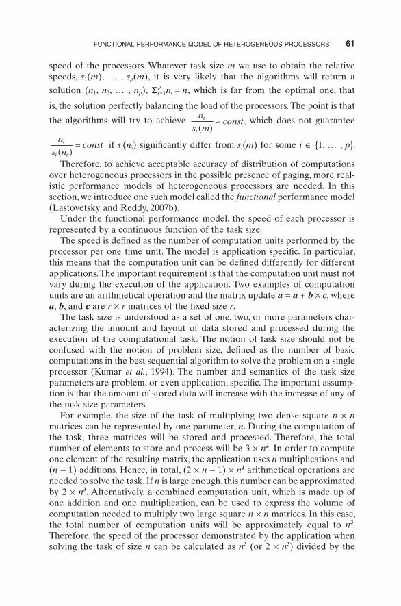
FUNCTIONAL PERFORMANCE MODEL OF HETEROGENEOUS PROCESSORS 61
speed of the processors. Whatever task size m we use to obtain the relative speeds, s 1 ( m ), … , s p ( m ), it is very likely that the algorithms will return a
solution ( n 1 , n 2 , … , n p ), Σ ip
in n= =1 , which is far from the optimal one, that
is, the solution perfectly balancing the load of the processors. The point is that
the algorithms will try to achieve
ns m
consti
i ( )≈ , which does not guarantee
n
s nconsti
i i( )≈ if s i ( n i ) signifi cantly differ from s i ( m ) for some i ∈ {1, … , p }.
Therefore, to achieve acceptable accuracy of distribution of computations over heterogeneous processors in the possible presence of paging, more real-istic performance models of heterogeneous processors are needed. In this section, we introduce one such model called the functional performance model (Lastovetsky and Reddy, 2007b ).
Under the functional performance model, the speed of each processor is represented by a continuous function of the task size.
The speed is defi ned as the number of computation units performed by the processor per one time unit. The model is application specifi c. In particular, this means that the computation unit can be defi ned differently for different applications. The important requirement is that the computation unit must not vary during the execution of the application. Two examples of computation units are an arithmetical operation and the matrix update a = a + b × c , where a , b , and c are r × r matrices of the fi xed size r .
The task size is understood as a set of one, two, or more parameters char-acterizing the amount and layout of data stored and processed during the execution of the computational task. The notion of task size should not be confused with the notion of problem size, defi ned as the number of basic computations in the best sequential algorithm to solve the problem on a single processor (Kumar et al. , 1994 ). The number and semantics of the task size parameters are problem, or even application, specifi c. The important assump-tion is that the amount of stored data will increase with the increase of any of the task size parameters.
For example, the size of the task of multiplying two dense square n × n matrices can be represented by one parameter, n . During the computation of the task, three matrices will be stored and processed. Therefore, the total number of elements to store and process will be 3 × n 2 . In order to compute one element of the resulting matrix, the application uses n multiplications and ( n − 1) additions. Hence, in total, (2 × n − 1) × n 2 arithmetical operations are needed to solve the task. If n is large enough, this number can be approximated by 2 × n 3 . Alternatively, a combined computation unit, which is made up of one addition and one multiplication, can be used to express the volume of computation needed to multiply two large square n × n matrices. In this case, the total number of computation units will be approximately equal to n 3 . Therefore, the speed of the processor demonstrated by the application when solving the task of size n can be calculated as n 3 (or 2 × n 3 ) divided by the
62 DISTRIBUTION OF COMPUTATIONS WITH NONCONSTANT PERFORMANCE MODELS
execution time of the application. This gives us a function from the set of natural numbers representing task sizes into the set of nonnegative real numbers representing the speeds of the processor, f: N → R + . The functional performance model of the processor is obtained by continuous extension of function f: N → R + to function g: R + → R + (f( n ) = g( n ) for any n from N ).
Another example is the task of multiplying two dense rectangular n × k and k × m matrices. The size of this task is represented by three parameters, n , k , and m . The total number of matrix elements to store and process will be ( n × k + k × m + n × m ). The total number of arithmetical operations needed to solve this task is (2 × ( k − 1)) × n × m . If k is large enough, this number can be approximated by 2 × k × n × m . Alternatively, a combined computation unit made up of one addition and one multiplication can be used, resulting in the total number of computation units approximately equal to k × n × m . There-fore, the speed of the processor exposed by the application when solving the task of size ( n , k , m ) can be calculated as k × n × m (or 2 × k × n × m ) divided by the execution time of the application. This gives us a function f: N 3 → R + , mapping task sizes to the speeds of the processor. The functional performance model of the processor is obtained by a continuous extension of function f: N 3 → R + to function g: R R+
3+ f→ ( ( ) = ( )n k m g n k m, , , , for any ( n , k , m ) from
N 3 ). Thus, under the functional model, the speed of the processor is represented
by a continuous function of the task size. Moreover, some further assumptions are made about the shape of the function. Namely, it is assumed that along each of the task size variables, either the function is monotonically decreasing or there exists point x such that
• on the interval [0, x ], the function is
� monotonically increasing, � concave, and � any straight line coming through the origin of the coordinate system
intersects the graph of the function in no more than one point; and • on the interval [ x , ∞ ), the function is monotonically decreasing.
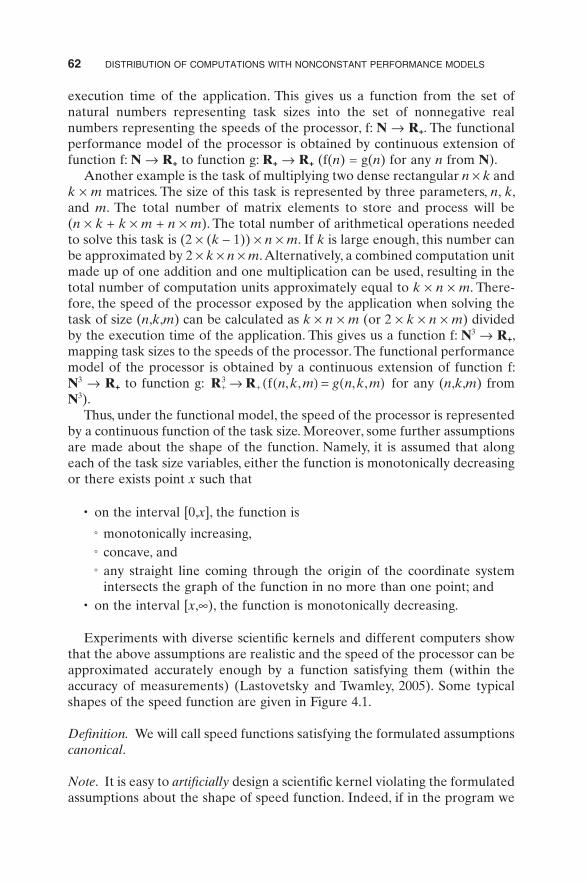
Experiments with diverse scientifi c kernels and different computers show that the above assumptions are realistic and the speed of the processor can be approximated accurately enough by a function satisfying them (within the accuracy of measurements) (Lastovetsky and Twamley, 2005 ). Some typical shapes of the speed function are given in Figure 4.1 .
Defi nition. We will call speed functions satisfying the formulated assumptions canonical .
Note . It is easy to artifi cially design a scientifi c kernel violating the formulated assumptions about the shape of speed function. Indeed, if in the program we
FUNCTIONAL PERFORMANCE MODEL OF HETEROGENEOUS PROCESSORS 63
use na ï ve matrix multiplication for some matrix sizes and highly effi cient ATLAS (Whaley, Petitet, and Dongarra, 2001 ) routine for the others, the resulting speed function will not be even continuous. We postulate that this is not the case for naturally designed scientifi c codes.
Some carefully designed codes such as ArrayOpsF (Fig. 4.1 (a)) and Matrix-MultAtlas (Fig. 4.1 (c)), which effi ciently use memory hierarchy, demonstrate quite a sharp and distinctive curve of dependence of the absolute speed on the task size. Their design manages to delay the appearance of page faults, minimizing their number for medium task sizes. However, because any design can only delay paging but not avoid it, the number of page faults will start
0
20
40
60
80
100
120
0 10,000,000 20,000,000 30,000,000 40,000,000 50,000,000 60,000,000 70,000,000 0 1000 2000 3000 4000 5000 6000 7000 8000 9000
Size of the array
(a) (b)
(c)
Abs
olut
e sp
eed
(meg
aflo
ps)
Comp3
Comp4
Comp2
Comp1
0
50
100
150
200
250
300
350
Size of the matrix
Abs
olut
e sp
eed
(meg
aflo
ps)
Comp3
Comp2
Comp1
Comp4
0
500
1000
1500
2000
2500
3000
3500
4000
0 1000 2000 3000 4000 5000 6000 7000 8000
Size of the matrix
Abs
olut
e sp
eed
(meg
aflo
ps)
Comp4
Comp2
Comp1
Figure 4.1. Shapes of the speed function for three different applications run on four heterogeneous processors. (a) ArrayOpsF: Arithmetic operations on three arrays of data, accessing memory in a contiguous manner, with an effi cient memory referencing pattern and use of cache. (b) MatrixMult: A naive implementation of the multiplication of two dense square matrices, with the result placed in a third matrix. Memory will be accessed in a noneffi cient manner. As a result, page faults start occurring for relatively small matrices, gradually increasing with the increase of the matrx size. (c) Matrix-MultATLAS: An effi cient implementation of matrix multiplication utilizing the dgemm BLAS routine, optimized using ATLAS .

64 DISTRIBUTION OF COMPUTATIONS WITH NONCONSTANT PERFORMANCE MODELS
growing like a snowball, beginning from some threshold value of the task size. For such codes, the speed of the processor can be approximated accurately enough by a unit step function. One potential advantage of modeling the processor speed by unit step functions is that parallel algorithms with such models might be obtained by straightforward extensions of parallel algorithms with constant models.
At the same time, application MatrixMult (Fig. 4.1 (b)), which implements a straightforward algorithm of multiplication of two dense square matrices and uses ineffi cient memory reference patterns, displays quite a smooth dependence of the speed on the task size. Page faults for this application start occurring much earlier than for its carefully designed counterpart, but the increase of their number will be much slower. A unit step function cannot accurately approximate the processor speed for such codes. Thus, if we want to have a single performance model covering the whole range of codes, the general functional model is a much better candidate than a model based on the unit step function.
4.2 DATA PARTITIONING WITH THE FUNCTIONAL PERFORMANCE MODEL OF HETEROGENEOUS PROCESSORS
In this section, we revisit some data partitioning problems that have been studied in Chapter 3 with constant performance models of heterogeneous processors. We will formulate and study them with the functional performance model.
We begin with the basic problem of partitioning a set of n (equal) elements between p heterogeneous processors. As we have seen in Chapter 3 , the problem is a generalization of the problem of distributing independent com-putation units over a unidimensional arrangement of heterogeneous proces-sors. The problem can be formulated as follows:
• Given a set of p processors P 1 , P 2 , … , P p , the speed of each of which is characterized by a real function, s i ( x )
• Partition a set of n elements into p subsets so that � There is one - to - one mapping between the partitions and the
processors
� The partitioning minimizes max i
i
i i
ns n( )
, where n i is the number of
elements allocated to processor P i (1 ≤ i ≤ p )
The motivation behind this formulation is obvious. If elements of the set represent computation units of equal size, then the speed of the processor can be understood as the number of computation units performed by the processor per one time unit. The speed depends on the number of units assigned to the processor and is represented by a continuous function s: R + → R + . As we
DATA PARTITIONING WITH THE FUNCTIONAL PERFORMANCE MODEL 65
assume that the processors perform their computation units in parallel, the overall execution time obtained with allocation ( n 1 , n 2 , … , n p ) will be given
by max ii
i i
ns n( )
. The optimal solution has to minimize the overall execution time.
Algorithm 4.1 (Lastovetsky and Reddy, 2007b ). Optimal distribution for n equal elements over p processors of speeds s 1 ( x ), s 2 ( x ), … , s p ( x ):
• Step 1: Initialization. We approximate the n i so that
ns n
consti
i i( )≈ and
n − 2 × p ≤ n 1 + n 2 + … + n p ≤ n . Namely, we fi nd n i such that either n xi i= ⎣ ⎦
or n xi i= ⎣ ⎦ − 1 for 1 ≤ i ≤ p , where
xs x
xs x
x
s xp
p p
1
1 1
2
2 2( )=
( )= =
( )… .
• Step 2: Refi ning. We iteratively increment some n i until n 1 + n 2 + … + n p = n .
Approximation of the n i (Step 1) is not that easy as in the case of constant
speeds s i of the processors when n i can be approximated as
s
sni
piΣ1
×⎢⎣⎢
⎥⎦⎥ (see
Section 3.1 ). The algorithm is based on the following observations:
• Let
xs x
xs x
x
s xp
p p
1
1 1
2
2 2( )=
( )= =
( )… .
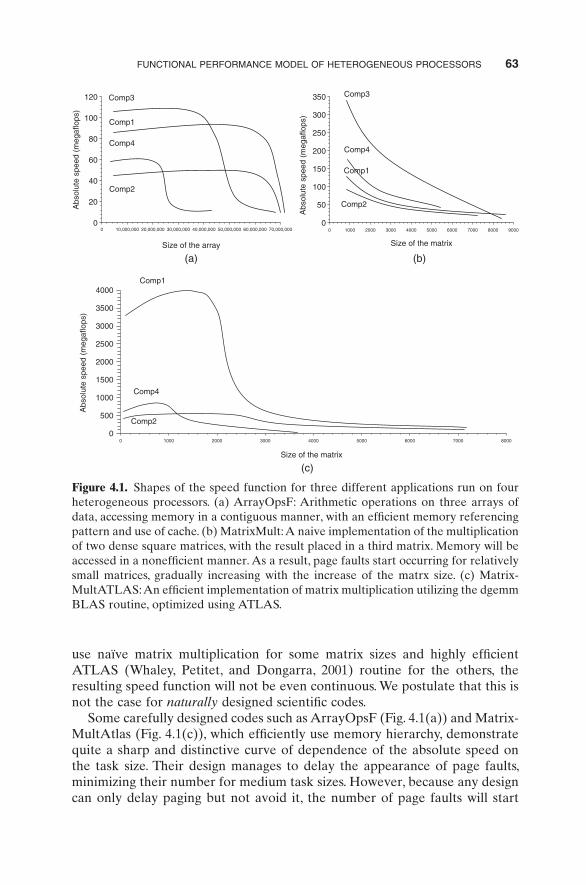
• Then all the points ( x 1 , s 1 ( x 1 )), ( x 2 , s 2 ( x 2 )), … , ( x p , s p ( x p )) will lie on a straight line passing through the origin of the coordinate system, being intersecting points of this line with the graphs of the speed functions of the processors. This is shown in Figure 4.2 .
s3(x1)
s1(x)
s2(x)x1 x2 x3 x4
s3(x)
s4(x)
Size of the problem
Abs
olut
e sp
eed
x1
s4(x2)
x2
s1(x3)
x3
s2(x4)
(x1, s3(x1))(x2, s4(x2))
(x3, s1(x3))(x4, s2(x4))
x4
Figure 4.2. “ Ideal ” optimal solution showing the geometric proportionality of the number of elements to the speed of the processor.
66 DISTRIBUTION OF COMPUTATIONS WITH NONCONSTANT PERFORMANCE MODELS
This algorithm is seeking for two straight lines passing through the origin of the coordinate system such that:
• The “ ideal ” optimal line (i.e., the line that intersects the speed graphs in points ( x 1 , s 1 ( x 1 )), ( x 2 , s 2 ( x 2 )), … , ( x p , s p ( x p )) such that
xs x
xs x
x
s xp
p p
1
1 1
2
2 2( )=
( )= =
( )… and x 1 + x 2 + … + x p = n ) lies between the
two lines.
• There is no more than one point with integer x coordinate on either of these graphs between the two lines.
Algorithm 4.2 (Lastovetsky and Reddy, 2007b ). Approximation of the n i so that either n xi i= ⎣ ⎦ or n xi i= ⎣ ⎦ − 1 for 1 ≤ i ≤ p , where
xs x
xs x
x
s xp
p p
1
1 1
2
2 2( )=
( )= =
( )… and x 1 + x 2 + … + x p = n :
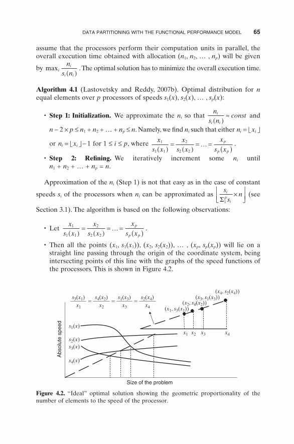
• Step 1. The upper line U is drawn through the points (0, 0) and
np
snp
i i, max ⎛⎝⎜
⎞⎠⎟
⎧⎨⎩
⎫⎬⎭
⎛⎝⎜
⎞⎠⎟
, and the lower line L is drawn through the points
(0, 0) and np
snp
i i, min ⎛⎝⎜
⎞⎠⎟
⎧⎨⎩
⎫⎬⎭
⎛⎝⎜
⎞⎠⎟ , as shown in Figure 4.3 .
• Step 2. Let xiU( ) and xi
L( ) be the coordinates of the intersection points of lines U and L with the function s i ( x ) (1 ≤ i ≤ p ). If there exists i ∈ {1, … , p } such that x xi
LiU( ) ( )− ≥ 1 then go to Step 3 else go to Step 5.
Figure 4.3. Selection of the initial two lines L and U . Here, n is the number of elements and p is the number of processors .

DATA PARTITIONING WITH THE FUNCTIONAL PERFORMANCE MODEL 67
• Step 3. Bisect the angle between lines U and L by the line M . Calculate coordinates xi
M( ) of the intersection points of the line M with the function s i ( x ) for 1 ≤ i ≤ p .
• Step 4. If Σ ip
iMx n=
( ) ≤1 then U = M else L = M . Go to Step 2. • Step 5. Approximate the n i so that n xi i
U= ⎢⎣ ⎥⎦( ) for 1 ≤ i ≤ p .
Proposition 4.1 (Lastovetsky and Reddy, 2007b ). Let functions s i ( x ) (1 ≤ i ≤ p ) be canonical speed functions. Then Algorithm 4.2 fi nds the n i such that either
n xi i= ⎣ ⎦ or n xi i= ⎣ ⎦ − 1 for 1 ≤ i ≤ p , where
xs x
xs x
x
s xp
p p
1
1 1
2
2 2( )=
( )= =
( )… and
x 1 + x 2 + … + x p = n . See Appendix B for proof.
Algorithm 4.3 (Lastovetsky and Reddy, 2007b ). Iterative incrementing of some n i until n 1 + n 2 + … + n p = n :
• Step 1. If n 1 + n 2 + … + n p < n then go to Step 2 else stop the algorithm.
• Step 2. Find k ∈ {1, … , p } such that
ns n
ns n
k
k kip i
i i
++( )
=++( )
⎧⎨⎩
⎫⎬⎭
=11
111min .
• Step 3. n k = n k + 1. Go to Step 1.
Note . It is worth to stress that Algorithm 4.3 cannot be used to search for the optimal solution beginning from an arbitrary approximation n i satisfying inequality n 1 + n 2 + … + n p < n , but only from the approximation found by Algorithm 4.2.
Proposition 4.2 (Lastovetsky and Reddy, 2007b ). Let the functions s i ( x ) (1 ≤ i ≤ p ) be canonical speed functions. Let ( n 1 , n 2 , … , n p ) be the approximation found by Algorithm 4.2. Then Algorithm 4.3 returns the optimal allocation.
See Appendix B for proof.
Defi nition. The heterogeneity of the set of p physical processors P 1 , P 2 , … , P p of respective speeds s 1 ( x ), s 2 ( x ), … , s p ( x ) is bounded if and only if there exists
a constant c such that max max
minx R
s xs x
c∈ +
( )( )
≤ , where s max ( x ) = max i s i ( x ) and
s min ( x ) = min i s i ( x ).
Proposition 4.3 (Lastovetsky and Reddy, 2007b ). Let speed functions s i ( x ) (1 ≤ i ≤ p ) be canonical and the heterogeneity of processors P 1 , P 2 , … , P p be bounded. Then, the complexity of Algorithm 4.2 can be bounded by O ( p × log 2 n ).
See Appendix B for proof.
68 DISTRIBUTION OF COMPUTATIONS WITH NONCONSTANT PERFORMANCE MODELS
Proposition 4.4. Let speed functions s i ( x ) (1 ≤ i ≤ p ) be canonical and the heterogeneity of proc essors P 1 , P 2 , … , P p be bounded. Then, the complexity of Algorithm 4.1 can be bounded O ( p × log 2 n ).
Proof . If ( n 1 , n 2 , … , n p ) is the approximation found by Algorithm 4.2, then n − 2 × p ≤ n 1 + n 2 + … + n p ≤ n and Algorithm 4.3 gives the optimal allocation in at most 2 × p steps of increment, so that the complexity of Algorithm 4.3 can be bounded by O ( p 2 ). This complexity is given by a na ï ve implementation of Algorithm 4.3. The complexity of this algorithm can be reduced down to O ( p × log 2 p ) by using ad hoc data structures. Thus, overall, the complexity of Algorithm 4.1 will be O ( p × log 2 p + p × log 2 n ) = O ( p × log 2 ( p × n )) . Since p < n , then log 2 ( p × n ) < log 2 ( n × n ) = log 2 ( n 2 ) = 2 × log 2 n . Thus, the complexity of Algorithm 4.1 can be bounded by O (2 × p × log 2 n ) = O ( p × log 2 n ). Proposition 4.4 is proved.
The low complexity of Algorithm 4.2 and, hence, of Algorithm 4.1 is mainly due to the bounded heterogeneity of the processors. This very property guar-antees that each bisection will reduce the space of possible solutions by a fraction that is lower bounded by some fi nite positive number independent of n . The assumption of bounded heterogeneity will be inaccurate if the speed of some processors becomes too slow for large n , effectively approaching zero.
In this case, Algorithm 4.2 may become ineffi cient. For example, if
s xx
ei x( ) −~
for large x , then the number of bisections of the angle will be proportional to n for large n , resulting in the complexity of O ( p × n ).
The fi rst approach to this problem is to use algorithms that are not that sensitive to the shape of speed functions for large task sizes. One such algo-rithm is obtained by a modifi cation of Algorithm 4.2 (Lastovetsky and Reddy, 2004a ).
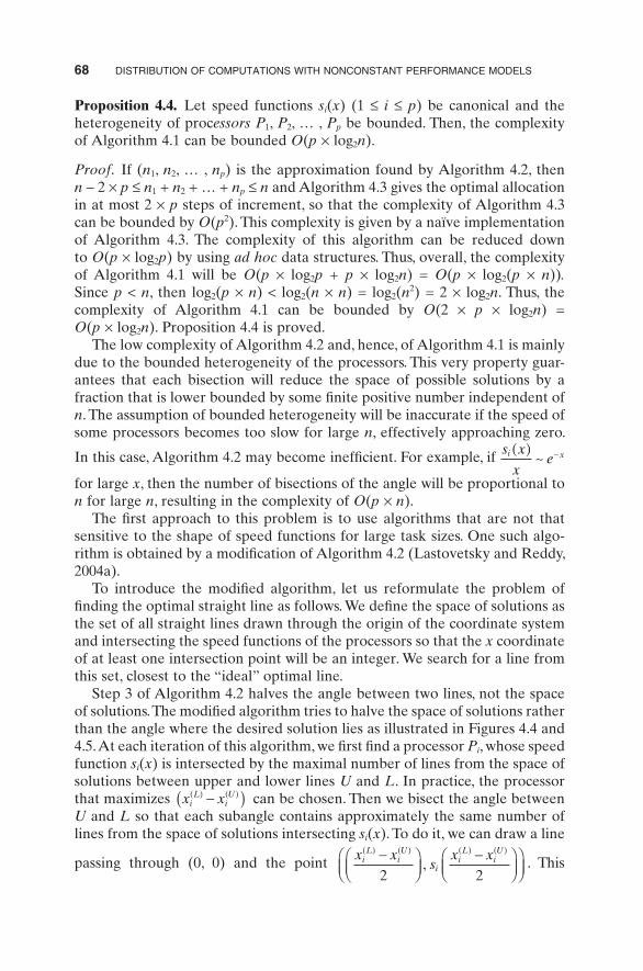
To introduce the modifi ed algorithm, let us reformulate the problem of fi nding the optimal straight line as follows. We defi ne the space of solutions as the set of all straight lines drawn through the origin of the coordinate system and intersecting the speed functions of the processors so that the x coordinate of at least one intersection point will be an integer. We search for a line from this set, closest to the “ ideal ” optimal line.
Step 3 of Algorithm 4.2 halves the angle between two lines, not the space of solutions. The modifi ed algorithm tries to halve the space of solutions rather than the angle where the desired solution lies as illustrated in Figures 4.4 and 4.5 . At each iteration of this algorithm, we fi rst fi nd a processor P i , whose speed function s i ( x ) is intersected by the maximal number of lines from the space of solutions between upper and lower lines U and L . In practice, the processor that maximizes x xi
LiU( ) ( )−( ) can be chosen. Then we bisect the angle between
U and L so that each subangle contains approximately the same number of lines from the space of solutions intersecting s i ( x ). To do it, we can draw a line
passing through (0, 0) and the point
x xs
x xiL
iU
iiL
iU( ) ( ) ( ) ( )−⎛
⎝⎜⎞⎠⎟
−⎛⎝⎜
⎞⎠⎟
⎛⎝⎜
⎞⎠⎟2 2
, . This
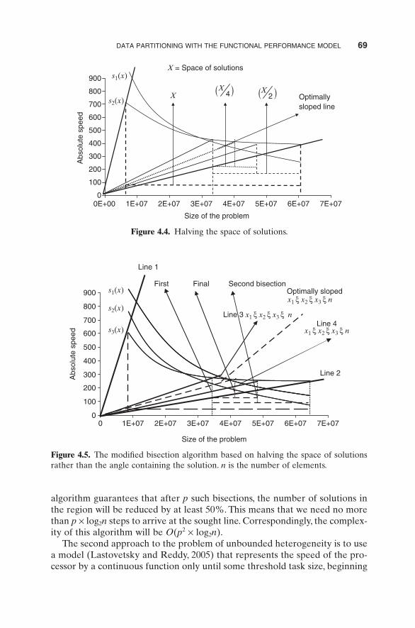
DATA PARTITIONING WITH THE FUNCTIONAL PERFORMANCE MODEL 69
algorithm guarantees that after p such bisections, the number of solutions in the region will be reduced by at least 50%. This means that we need no more than p × log 2 n steps to arrive at the sought line. Correspondingly, the complex-ity of this algorithm will be O ( p 2 × log 2 n ).
The second approach to the problem of unbounded heterogeneity is to use a model (Lastovetsky and Reddy, 2005 ) that represents the speed of the pro-cessor by a continuous function only until some threshold task size, beginning
0
100
200
300
400
500
600
700
800
900
0E+00 1E+07 2E+07 3E+07 4E+07 5E+07 6E+07 7E+07
Size of the problem
Abs
olut
e sp
eed
s1(x)
s2(x)X 2
X4X
X = Space of solutions
Optimally sloped line
)()(
Figure 4.4. Halving the space of solutions.
0
100
200
300
400
500
600
700
800
900
0 1E+07 2E+07 3E+07 4E+07 5E+07 6E+07 7E+07
Size of the problem
Abs
olut
e sp
eed
Line 1
Line 2
Line 3 x1 ξ x2 ξ x3 ξ n
x1 ξ x2 ξ x3 ξ n
x1 ξ x2 ξ x3 ξ n
First Second bisection
Line 4
Final Optimally slopeds1(x)
s2(x)
s3(x)
Figure 4.5. The modifi ed bisection algorithm based on halving the space of solutions rather than the angle containing the solution. n is the number of elements.
70 DISTRIBUTION OF COMPUTATIONS WITH NONCONSTANT PERFORMANCE MODELS
from which the speed of the processor becomes so low that it makes no sense to use it for computations. Correspondingly, the model approximates the speed of the processor by zero for all task sizes greater than this threshold value. Data partitioning with this model is discussed in Section 4.3 .
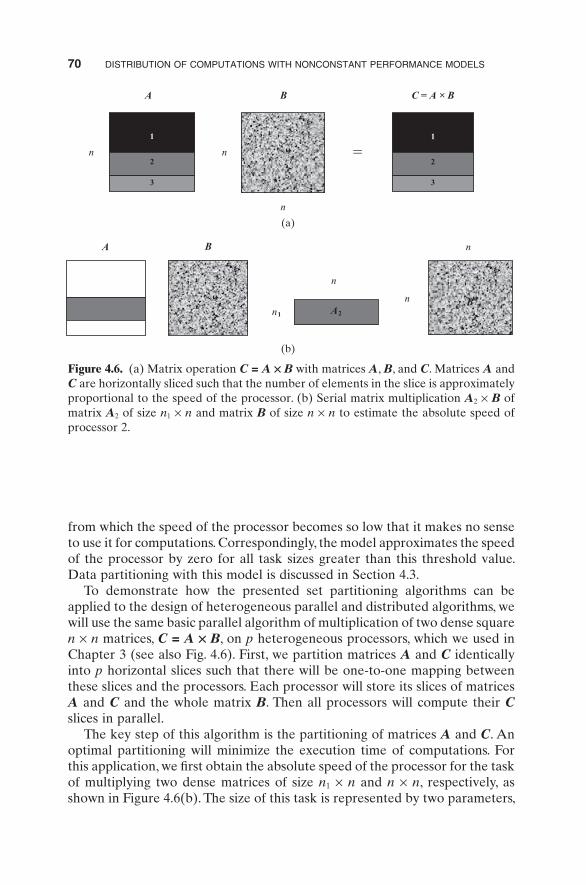
To demonstrate how the presented set partitioning algorithms can be applied to the design of heterogeneous parallel and distributed algorithms, we will use the same basic parallel algorithm of multiplication of two dense square n × n matrices, C = A × B , on p heterogeneous processors, which we used in Chapter 3 (see also Fig. 4.6 ). First, we partition matrices A and C identically into p horizontal slices such that there will be one - to - one mapping between these slices and the processors. Each processor will store its slices of matrices A and C and the whole matrix B . Then all processors will compute their C slices in parallel.
The key step of this algorithm is the partitioning of matrices A and C . An optimal partitioning will minimize the execution time of computations. For this application, we fi rst obtain the absolute speed of the processor for the task of multiplying two dense matrices of size n 1 × n and n × n , respectively, as shown in Figure 4.6 (b ). The size of this task is represented by two parameters,
(a)
(b)
1
2
3
A B C = A × B
=n
n
n
1
2
3
A B
n
B
n
n1
n A2
Figure 4.6. (a) Matrix operation C = A × B with matrices A , B , and C . Matrices A and C are horizontally sliced such that the number of elements in the slice is approximately proportional to the speed of the processor. (b) Serial matrix multiplication A 2 × B of matrix A 2 of size n 1 × n and matrix B of size n × n to estimate the absolute speed of processor 2.
DATA PARTITIONING WITH THE FUNCTIONAL PERFORMANCE MODEL 71
Abs
olut
e sp
eed
(meg
aflo
ps)
X5
8
1000 2000 3000 4000 5000 6000 7000 8000 9000
02000
40006000
800010,000
10,000
7
6
5
4
Abs
olut
e sp
eed
(meg
aflo
ps)
3
2
1
0
6000
5000
4000
3000
2000
1000
1000 2000 3000 4000 5000 6000 70008000 900010,00010,000
5000n1
n1
n1
nn
×104
X1
(a)
0
Abs
olut
e sp
eed
(meg
aflo
ps)
0
90
80
70
60
50
40
30
20
10002000
40006000
800010,000
6000
1000 2000 3000 4000 5000 6000 7000 8000 9000 10,000
Rel
ativ
e sp
eed
n1
n
n
(b)
(c)
7000 8000 9000 10,000 8000 6000 4000 2000 0
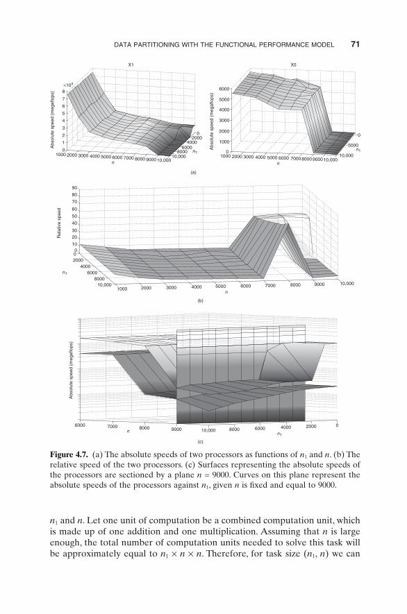
Figure 4.7. (a) The absolute speeds of two processors as functions of n 1 and n . (b) The relative speed of the two processors. (c) Surfaces representing the absolute speeds of the processors are sectioned by a plane n = 9000. Curves on this plane represent the absolute speeds of the processors against n 1 , given n is fi xed and equal to 9000.
n 1 and n . Let one unit of computation be a combined computation unit, which is made up of one addition and one multiplication. Assuming that n is large enough, the total number of computation units needed to solve this task will be approximately equal to n 1 × n × n . Therefore, for task size ( n 1 , n ) we can
72 DISTRIBUTION OF COMPUTATIONS WITH NONCONSTANT PERFORMANCE MODELS
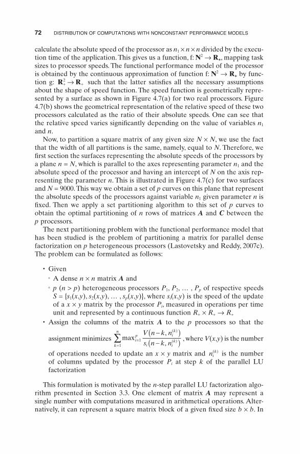
calculate the absolute speed of the processor as n 1 × n × n divided by the execu-tion time of the application. This gives us a function, f: N 2 → R + , mapping task sizes to processor speeds. The functional performance model of the processor is obtained by the continuous approximation of function f: N 2 → R + by func-tion g: R R+ +→2 such that the latter satisfi es all the necessary assumptions about the shape of speed function. The speed function is geometrically repre-sented by a surface as shown in Figure 4.7 (a) for two real processors. Figure 4.7 (b) shows the geometrical representation of the relative speed of these two processors calculated as the ratio of their absolute speeds. One can see that the relative speed varies signifi cantly depending on the value of variables n 1 and n .
Now, to partition a square matrix of any given size N × N , we use the fact that the width of all partitions is the same, namely, equal to N . Therefore, we fi rst section the surfaces representing the absolute speeds of the processors by a plane n = N , which is parallel to the axes representing parameter n 1 and the absolute speed of the processor and having an intercept of N on the axis rep-resenting the parameter n . This is illustrated in Figure 4.7 (c) for two surfaces and N = 9000 . This way we obtain a set of p curves on this plane that represent the absolute speeds of the processors against variable n 1 given parameter n is fi xed. Then we apply a set partitioning algorithm to this set of p curves to obtain the optimal partitioning of n rows of matrices A and C between the p processors.
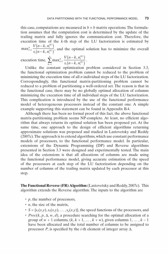
The next partitioning problem with the functional performance model that has been studied is the problem of partitioning a matrix for parallel dense factorization on p heterogeneous processors (Lastovetsky and Reddy, 2007c ). The problem can be formulated as follows:
• Given � A dense n × n matrix A and � p ( n > p ) heterogeneous processors P 1 , P 2 , … , P p of respective speeds
S = { s 1 ( x , y ), s 2 ( x , y ), … , s p ( x , y )}, where s i ( x , y ) is the speed of the update of a x × y matrix by the processor P i , measured in operations per time unit and represented by a continuous function R + × R + → R +
• Assign the columns of the matrix A to the p processors so that the
assignment minimizes max,
,ip i
k
i ik
k
n V n k n
s n k n=
( )
( )=
−( )−( )∑ 1
1
, where V ( x , y ) is the number
of operations needed to update an x × y matrix and nik( ) is the number
of columns updated by the processor P i at step k of the parallel LU factorization
This formulation is motivated by the n - step parallel LU factorization algo-rithm presented in Section 3.3 . One element of matrix A may represent a single number with computations measured in arithmetical operations. Alter-natively, it can represent a square matrix block of a given fi xed size b × b . In
DATA PARTITIONING WITH THE FUNCTIONAL PERFORMANCE MODEL 73
this case, computations are measured in b × b matrix operations. The formula-tion assumes that the computation cost is determined by the update of the trailing matrix and fully ignores the communication cost. Therefore, the execution time of the k - th step of the LU factorization is estimated by
max,
,ip i
k
i ik
V n k n
s n k n=
( )
( )
−( )−( )1 , and the optimal solution has to minimize the overall
execution time, max,
,ip i
k
i ik
k
n V n k n
s n k n=
( )
( )=
−( )−( )∑ 1
1
.
Unlike the constant optimization problem considered in Section 3.3 , the functional optimization problem cannot be reduced to the problem of minimizing the execution time of all n individual steps of the LU factorization. Correspondingly, this functional matrix - partitioning problem cannot be reduced to a problem of partitioning a well - ordered set. The reason is that in the functional case, there may be no globally optimal allocation of columns minimizing the execution time of all individual steps of the LU factorization. This complication is introduced by the use of the functional performance model of heterogeneous processors instead of the constant one. A simple example supporting this statement can be found in Appendix B.4 .
Although there has been no formal proof of this fact, the above functional matrix - partitioning problem seems NP - complete. At least, no effi cient algo-rithm that always returns its optimal solution has been proposed yet. At the same time, one approach to the design of effi cient algorithms returning approximate solutions was proposed and studied in Lastovetsky and Reddy (2007c) . The approach is to extend algorithms, which use constant performance models of processors, to the functional performance model. In particular, extensions of the Dynamic Programming (DP ) and Reverse algorithms presented in Section 3.3 were designed and experimentally tested. The main idea of the extensions is that all allocations of columns are made using the functional performance model, giving accurate estimation of the speed of the processors at each step of the LU factorization depending on the number of columns of the trailing matrix updated by each processor at this step.
The Functional Reverse (FR) Algorithm (Lastovetsky and Reddy, 2007c ). This algorithm extends the Reverse algorithm. The inputs to the algorithm are
• p , the number of processors, • n , the size of the matrix, • S = { s 1 ( x , y ), s 2 ( x , y ), … , s p ( x , y )}, the speed functions of the processors, and • Proc ( k , p , Δ , w , d ), a procedure searching for the optimal allocation of a
group of w + 1 columns, ( k , k + 1, … , k + w ), given columns 1, … , k − 1 have been allocated and the total number of columns to be assigned to processor P i is specifi ed by the i - th element of integer array Δ .

74 DISTRIBUTION OF COMPUTATIONS WITH NONCONSTANT PERFORMANCE MODELS
The output d is an integer array of size n , the i - th element of which contains the index of the processor to which the column i is assigned.
The algorithm can be summarized as follows:
( d 1 , … , d n )=(0, … ,0);
w =0;
( n 1 , … , n p )=HSPF( p , n , S );
for ( k =1; k < n ; k = k +1) { ( ′n1 , … , ′np )= HSPF( p , n - k , S );
if ( w ==0)
then if (( ∃ ! j ∈ [1, p ])( n j == ′nj+1) ∧ ( ∀ i ≠ j )( n i == ′nj)) then { d k = j ; ( n 1 , … , n p ) = ( ′n1 , … , ′np );}
else w =1;
else if (( ∃ i ∈ [1, p ])( n i < ′ni )) then w = w +1;
else {
for ( i =1; i ≤ p ; i = i +1) { Δ i = n i − ′ni ;} Proc(k, p, Δ , w, d) ; ( n 1 , … , n p ) = ( ′n1 , … , ′np );
w =0;
}
}
if (( ∃ i ∈ [1, p ])( n i = 1)) then d n = i ;
Here, HSPF( p , m , S ) (HSPF stands for heterogeneous set partitioning using the functional model of processors ) returns the optimal distribution of a set of m equal elements over p heterogeneous processors P 1 , P 2 , … , P p of respective speeds S = { s 1 ( m , y ), s 2 ( m , y ), … , s p ( m , y )} using Algorithm 4.1. The distributed elements represent columns of the m × m trailing matrix at step ( n − m ) of the LU factorization. Function f i ( y ) = s i ( m , y ) represents the speed of processor P i depending on the number of columns of the trailing matrix, y , updated by the processor at the step ( n − m ) of the LU factorization. Figure 4.8 gives a geometrical interpretation of this step of the matrix - parttioning algorithm:
1. Surfaces z i = s i ( x , y ) representing the absolute speeds of the processors are sectioned by the plane x = n − k ( as shown on Fig. 4.8 (a) for three surfaces). A set of p curves on this plane (as shown in Fig. 4.8 (b)) will represent the absolute speeds of the processors against variable y , given parameter x is fi xed.
2. Algorithm 4.1 is applied to this set of curves to obtain an optimal distri-bution of columns of the trailing matrix.

DATA PARTITIONING WITH THE FUNCTIONAL PERFORMANCE MODEL 75
Proposition 4.5. If assignment of a column panel is performed at each step of the algorithm, the FR algorithm returns the optimal allocation.
Proof . If a column panel is assigned at each iteration of the FR algorithm, then the resulting allocation will be optimal by design. Indeed, in this case, the
600500
Abs
olut
e sp
eed
(meg
aflo
ps)
400300200100
×104×104
n2
n1
00
0.51
1.52
2.53
3.5 3(a)
2.52
1.51
0.5
hcl02hcl09hcl11Plane
0
×104n2
×104
n1
(b)
600500
Abs
olut
e sp
eed
(meg
aflo
ps)
400300200100
00
0.51
1.52
2.53
3.5 2.82.6
2.42.2
21.8
1.61.4
1.21
Figure 4.8. (a) Three surfaces representing the absolute speeds of three processors (hcl02, hcl09, hcl11) are sectioned by a plane x = m . (b) Curves on the plane represent the absolute speeds of the processors against variable y , given parameter x is fi xed . (See color insert.)

76 DISTRIBUTION OF COMPUTATIONS WITH NONCONSTANT PERFORMANCE MODELS
distribution of column panels over the processors will be produced by the HSPF, and hence, be optimal for each step of the LU factorization.
Proposition 4.6. If the speed of the processor is represented by a constant function of problem size, the FR algorithm returns the optimal allocation.
Proof . If the speed of the processor is represented by a constant function of problem size, the FR algorithm is functionally equivalent to the reverse algo-rithm presented earlier. We have already proved that the reverse algorithm returns the optimal allocation when the constant performance model of het-erogeneous processors is used.
Proposition 4.7. Let the functions s i ( x , y ) (1 ≤ i ≤ p ) be canonical speed func-tions for any fi xed x (i.e., along variable y ) and the heterogeneity of processors P 1 , P 2 , … , P p be bounded. Then, if assignment of a column panel is performed at each step of the algorithm, the complexity of the FR algorithm can be bounded by O ( p × n × log 2 n ).
Proof . At each iteration of this algorithm, we apply the HSPF. Intersection of p surfaces by a plane to produce p curves will be of complexity O ( p ). Application of Algorithm 4.1 to these curves will be of complexity bounded by O ( p × log 2 n ) (Proposition 4.4). Testing the condition ∃ ∈[ ]( ) == ′ +( ) ∧ ∀ ≠( ) == ′( )! ,j p n n i j n nj j i i1 1 is of complexity O ( p ). Since there are n such iterations, the overall complexity of the algorithm will be bounded by n × O ( p × log 2 n ) + n × O ( p ) + n × O ( p ) = O ( p × n × log 2 n ). End of proof of Proposition 4.7 .
If the FR algorithm does not assign a column at each iteration of its main loop, then the optimality of the returned allocation is not guaranteed. The reason is that when we are forced to allocate a group of columns, ( k , k + 1, … , k + w ), then even if procedure Proc fi nds a locally optimal allocation, minimiz-ing the sum of the execution times of the steps k , k + 1, … , k + w of the LU factorization (given columns 1, … , k − 1 have been allocated), this allocation may not minimize the global execution time. Hence, suboptimal allocations of the group of columns may be as good, or even better, as the exact optimal allocation. Therefore, in practice, it does not make much sense to use an exact but expansive algorithm in the implementation of procedure Proc . It has been shown (Lastovetsky and Reddy, 2007c ) that many simple approximate algo-rithms of low complexity, which do not change the upper bound O ( p × n × log 2 n ) of the overall complexity fo the FR algorithm, return group allocations that are, in average, as good as exact optimal allocations.
The Functional DP (FDP) Algorithm. This algorithm extends the DP algo-rithm. The inputs to the algorithm are
• p , the number of processors, • n , the size of the matrix, and
OTHER NONCONSTANT PERFORMANCE MODELS OF HETEROGENEOUS PROCESSORS 77
• S = { s 1 ( x , y ), s 2 ( x , y ), … , s p ( x , y )}, the speed functions of the processors.
The outputs are
• c , an integer array of size p , the i - th element of which contains the number of column panels assigned to processor P i , and
• d , an integer array of size n , the i - th element of which contains the index of the processor to which the column panel i is assigned.
The algorithm can be summarized as follows:
( c 1 , … , c p )=(0, … ,0);( d 1 , … , d n )=(0, … ,0); for ( k =1; k ≤ n ; k = k +1) { Cost min = ∞ ; ( n 1 , … , n p )=HSPF( p , k , S ); for ( i =1; i ≤ p ; i ++) { Cost=( c i +1)/ n i ; if (Cost < Cost min ) { Cost min = Cost; j = i ;} } d n - k +1 = j ; c j = c j +1;}
Proposition 4.8. If the functions s i ( x , y ) (1 ≤ i ≤ p ) are canonical speed func-tions for any fi xed x (i.e., along variable y ) and the heterogeneity of processors P 1 , P 2 , … , P p is bounded, the complexity of the FDP algorithm can be bounded by O ( p × n × log 2 n ).
Proof . The complexity of HSPF is O ( p × log 2 n ). The complexity of the inner for loop is O ( p ). Therefore, the complexity of one iteration of the main loop of this algorithm will be O ( p × log 2 n ) + O ( p ). Since there are n iterations, the complexity of the algorithm can be upper bounded by n × ( O ( p × log 2 n ) + O ( p )) = O ( p × n × log 2 n ). End of proof of Proposition 4.8 .
Thus, we see that the FR and FDP algorithms have the same complexity. At the same time, the FR algorithm has much more room for optimization as it does not have to assign a column at each iteration. Therefore, column alloca-tions returned by the FR algorithm will be closer to the optimal allocation, resulting in faster LU factorization. Experimental results validating this state-ment are presented in Lastovetsky and Reddy (2007c) .
4.3 OTHER NONCONSTANT PERFORMANCE MODELS OF HETEROGENEOUS PROCESSORS
4.3.1 Stepwise Functional Model
We have noted in Section 4.1 that for some scientifi c codes, which effi ciently use memory hierarchy and demonstrate a sharp and distinctive curve of
78 DISTRIBUTION OF COMPUTATIONS WITH NONCONSTANT PERFORMANCE MODELS
dependence of the absolute speed on the task size, the speed of the processor can be approximated by a unit step function. Such a model was also studied in Drozdowski and Wolniewicz (2003) . More precisely, under this model, the performance of the processor is characterized by the execution time of the task, represented by a piecewise linear function of its size. The problem of asymptotically optimal partitioning a set was formulated with this model as a linear programming problem. As such, it relies on the state of the art in linear programming. Currently, little is known (especially, theoretically) about practi-cal and effi cient algorithms for the linear programming problem. Moreover, if the unknown variables in the linear programming problem are all required to be integers, then the problem becomes an integer linear programming problem, which is known to be NP - hard in many practical situations. This means that the linear programming model can hardly be used in the design of effi cient algorithms returning the optimal exact solution of the set - partitioning problem.
4.3.2 Functional Model with Limits on Task Size
We have seen in Section 4.2 that the functional performance model can become ineffi cient if the speed of some processors is too slow for large task sizes, effectively approaching zero. In addition, it will be prohibitively expansive to build the model for large task sizes. To deal with the problems, a modifi ed functional model (Lastovetsky and Reddy, 2005 ) can be used in this case. This model represents the speed of the processor by a continuous function only until some threshold task size, beginning from which the speed of the proces-sor becomes so low that it makes no sense to use it for computations. Corre-spondingly, the model approximates the speed of the processor by zero for all task sizes greater than this threshold value. The basic problem of partitioning a set of n (equal) elements between p heterogeneous processors has been formulated and solved with this model (Lastovetsky and Reddy, 2005 ). The problem is formulated as follows:
• Given � A set of p processors P = { P 1 , P 2 , … , P p }, the speed of which is charac-
terized by real functions S = { s 1 ( x ), s 2 ( x ), … , s p ( x )} � Upper bounds B = { b 1 , … , b p ) limiting the number of elements allocated
to processors P • Partition a set of n elements into p subsets so that
� There is one - to - one mapping between the partitions and the processors
� n i ≤ b i , where n i is the number of elements allocated to processor P i (1 ≤ i ≤ p )
� The partitioning minimizes max i
i
i i
ns n( )
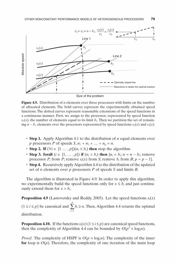
Algorithm 4.4. Optimal distribution for n equal elements over p processors P of speeds S and limits B :
OTHER NONCONSTANT PERFORMANCE MODELS OF HETEROGENEOUS PROCESSORS 79
• Step 1. Apply Algorithm 4.1 to the distribution of n equal elements over p processors P of speeds S , n 1 + n 2 + … + n p = n .
• Step 2. If ( ∀ i ∈ {1 … , p })( n i ≤ b i ) then stop the algorithm. • Step 3. forall ( i ∈ {1, … , p }) if ( n i > b i ) then { n i = b i ; n = n − b i ; remove
processor P i from P ; remove s i ( x ) from S ; remove b i from B ; p = p − 1}. • Step 4. Recursively apply Algorithm 4.4 to the distribution of the updated
set of n elements over p processors P of speeds S and limits B .
The algorithm is illustrated in Figure 4.9 . In order to apply this algorithm, we experimentally build the speed functions only for x ≤ b i and just continu-ously extend them for x > b i .
Proposition 4.9 (Lastovetsky and Reddy, 2005 ). Let the speed functions s i ( x )
(1 ≤ i ≤ p ) be canonical and
b nii
p
=∑ ≥
1
. Then, Algorithm 4.4 returns the optimal
distribution.
Proposition 4.10. If the functions s i ( x ) (1 ≤ i ≤ p ) are canonical speed functions, then the complexity of Algorithm 4.4 can be bounded by O ( p 2 × log 2 n ).
Proof . The complexity of HSPF is O ( p × log 2 n ). The complexity of the inner for loop is O ( p ). Therefore, the complexity of one iteration of the main loop
Size of the problem
Abs
olut
e sp
eed
s1(x)
s2(x)x2
s3(x)x3
x2
x2 + x3 = n – b1, =
x3
b2
b1
b3
s2(x)
s3(x)
Line 1
Line 2
Optimally sloped line
Bisections to obtain the optimal solution
Figure 4.9. Distribution of n elements over three processors with limits on the number of allocated elements. The bold curves represent the experimentally obtained speed functions. The dotted curves represent reasonable extensions of the speed functions in a continuous manner. First, we assign to the processor, represented by speed function s 1 ( x ), the number of elements equal to its limit b 1 . Then we partition the set of remain-ing n − b 1 elements over the processors represented by speed functions s 2 ( x ) and s 3 ( x ).
80 DISTRIBUTION OF COMPUTATIONS WITH NONCONSTANT PERFORMANCE MODELS
of this algorithm will be O ( p × log 2 n ) + O ( p ). Since there are n iterations, the complexity of the algorithm can be upper bounded by n × ( O ( p × log 2 n ) + O ( p )) = O ( p × n × log 2 n ). End of proof of Proposition 4.8 .
Application of the modifi ed functional model and Algorithm 4.4 is quite straightforward. Namely, they can seamlessly replace the functional model and Algorithm 4.1 in all presented algorithms where the solution of the set - partitioning problem is used as a basic building block.
4.3.3 Band Model
We have discussed in Chapters 1 and 2 that in general - purpose local and global networks integrated into the Internet, most computers periodically run some routine processes interacting with the Internet, and some computers act as servers for other computers. This results in constant unpredictable fl uctuations in the workload of processors in such a network. This changing transient load will cause fl uctuations in the speed of processors, in that the speed of the processor will vary when measured at different times while executing the same task. The natural way to represent the inherent fl uctuations in the speed is to use a speed band rather than a speed function. The width of the band charac-terizes the level of fl uctuation in the performance due to changes in load over time. Although some research on the band performance model and its use in the design of heterogeneous algorithms have been done (Higgins and Lastovetsky, 2005 ; Lastovetsky and Twamley, 2005 ), very little is known about the effectiveness and effi ciency of data partitioning algorithms at this point.