Embed Size (px)
Citation preview
Preprint typeset in JHEP style - HYPER VERSION
Higher Gauge Theory II: 2-Connections
John Baez
Department of Mathematics
University of California
Riverside, CA 92521, USA
Email: [email protected]
Urs Schreiber
Fachbereich Mathematik
Universitat Hamburg
Hamburg, 20146, Germany
Email: [email protected]
Abstract: Connections and curvings on gerbes are beginning to play a vital role in dif-
ferential geometry and theoretical physics — first abelian gerbes, and more recently non-
abelian gerbes and the twisted nonabelian gerbes introduced by Aschieri and Jurco in their
study of M-theory. These concepts can be elegantly understood using the concept of ‘2-
bundle’ recently introduced by Bartels. A 2-bundle is a generalization of a bundle in which
the fibers are categories rather than sets. Here we introduce the concept of a ‘2-connection’
on a principal 2-bundle. We describe principal 2-bundles with connection in terms of local
data, and show that under certain conditions this reduces to the cocycle data for twisted
nonabelian gerbes with connection and curving subject to a certain constraint — namely,
the vanishing of the ‘fake curvature’, as defined by Breen and Messing. This constraint
also turns out to guarantee the existence of ‘2-holonomies’: that is, parallel transport over
both curves and surfaces, fitting together to define a 2-functor from the ‘path 2-groupoid’
of the base space to the structure 2-group. We give a general theory of 2-holonomies and
show how they are related to ordinary parallel transport on the path space of the base
manifold.
Draft last modified 1/4/2008 – 13:14; current version at http://math.ucr.edu/home/baez/2conn.pdf
DR
AFT
Contents
1. Introduction 2
1.1 Nonabelian Surface Holonomies in Physics 2
1.2 Higher Gauge Theory 3
1.3 Outline of Results 8
1.4 Structure of the Paper 12
2. Preliminaries 13
2.1 Internalization 13
2.2 2-Spaces 16
2.3 Lie 2-Groups 18
2.4 Lie 2-Algebras 23
2.5 Nonabelian Gerbes 25
3. 2-Bundles 30
3.1 Locally Trivial 2-Bundles 30
3.2 2-Bundles in Terms of Local Data 31
4. 2-Connections 37
4.1 Path Groupoids and 2-Groupoids 37
4.2 Holonomy Functors and 2-Functors 39
5. 2-Connections from Local Data 45
5.1 Definition on Single Overlaps 45
5.2 Transition Law on Double Overlaps 47
5.3 Transition Law on Triple Overlaps 49
6. 2-Connections in Terms of Connections on Path Space 52
6.1 Connections on Smooth Spaces 52
6.2 More stuff... 55
6.3 The Standard Connection 1-Form on Path Space 57
6.4 Path Space Line Holonomy and Gauge Transformations 61
6.5 The Local 2-Holonomy Functor 64
7. Appendix: Smooth Spaces 69
– 1 –
Draft last modified 1/4/2008 – 13:14; current version at http://math.ucr.edu/home/baez/2conn.pdf
DR
AFT
1. Introduction
The concept of ‘connection’ lies at the very heart of modern physics, and it is central
to much of modern mathematics. A connection describes parallel transport along curves.
Motivated both by questions concerning M-theory (see §1.1) and ideas from higher category
theory (§1.2), we seek to describe parallel transport along surfaces. After describing these
motivations, we outline our results (§1.3) and sketch the structure of this paper (§1.4).
Readers intimidated by the length of this paper may prefer to read a summary of results
[5].
1.1 Nonabelian Surface Holonomies in Physics
In the context of M-theory (the only partially understood expected completion of string
theory), 2- and 5-dimensional surfaces in 10-dimensional space are believed to play a fun-
damental role. These are called ‘2-branes’ and ‘5-branes’, respectively. The general config-
uration of 2-branes and 5-branes involves 2-branes having boundaries that are attached to
5-branes. This is a higher-dimensional analogue of how open strings may end on various
types of branes in string theory. So, let us recall what happens in that simpler case.
When an open string ends on a single brane, its end acts like a point particle coupled
to a 1-form, or more precisely, to a U(1) connection. However, it is also possible for the
end of a string to mimic a point particle coupled to a nonabelian gauge field. This happens
when the string ends on a number of branes that are coincident, or ‘stacked’. When an
open string ends on a stack of n branes, its end acts like a point particle coupled to a U(n)
connection, or more generally a connection on some bundle whose structure group consists
of n × n matrices. The reason is that the action for the string involves the holonomy of
this connection along the curve traced out by the motion of the string’s endpoint as time
passes.
It is natural to hope that something similar happens when a 2-brane ends on a 5-brane
or a stack of 5-branes. Indeed, it is already known that when a 2-brane ends on a single
5-brane, it acts like a string coupled to a 2-form — or more precisely, to a connection on a
U(1) gerbe. (Just as a connection on a U(1) bundle can be locally identified with a 1-form,
but not globally, so a connection on a U(1) gerbe can be locally but not globally identified
with a 2-form.)
Similarly, we expect that a 2-brane ending on a stack of coinciding 5-branes should
behave like a string coupled to a Lie-algebra-valued 2-form — or more precisely, to a
connection on a nonabelian gerbe. The theory of such connections is under development,
and its application to this problem have already been considered [13, 14, 15]. However,
for this application to work, the action for a 2-brane ending on a stack of 5-branes should
involve some sort of ‘holonomy’ of this kind of connection over the 2-dimensional surface
traced out by the motion of the 2-brane’s boundary. For this, we need a concept of
‘nonabelian surface holonomy’.
It is well understood how connections on abelian gerbes give rise to a notion of abelian
surface holonomy, but for nonabelian gerbes so far no concept of surface holonomy has
been defined. In fact, using 2-groups it is straightforward to come up with a local version
– 2 –
Draft last modified 1/4/2008 – 13:14; current version at http://math.ucr.edu/home/baez/2conn.pdf
DR
AFT
of this notion. This has already been done in a discretized setting — a categorified version
of lattice gauge theory [9]. However, to construct a well-defined action for a 2-brane ending
on a stack of 5-branes, it is crucial to take care of global issues.
For these reasons, a globally defined notion of nonabelian surface holonomy seems to
be a necessary prerequisite for fully understanding the fundamental objects of M-theory.
In this paper we present such a notion, which we call ‘2-holonomy’.
In fact, this concept is interesting for ordinary field theory as well, quite independently
of whether strings really exist. Configurations of membranes ending on a stack of 5-branes
can alternatively be described in terms of certain (super)conformally invariant field theories
involving Lie-algebra-valued 2-form fields defined on the six-dimensional manifold traced
out by the 5-branes. When these field theories are compactified on a torus they give rise
to (super)Yang-Mills theory in four dimensions. In this context, the famous Montonen-
Olive SL(2,Z) duality exhibited by this 4-dimensional gauge theory should arise simply
from the modular transformations on the internal torus, which act as symmetries of the
conformally invariant six-dimensional theory. From this point of view, nonabelian 2-form
gauge theory in six dimensions appears as a tool for understanding ordinary gauge theory
in four dimensions.
It is interesting to note that these six-dimensional theories require the curvature 3-
form of the 2-form field to be self-dual with respect to the Hodge star operator. In the
nonabelian case this is subtle, because this 3-form should obey the local transition laws
for nonabelian gerbes, which are not — at least not in any obvious way — compatible
with self-duality in general, since they involve corrections to a covariant transformation
of the 3-form. The only obvious solution to this compatibility problem is to require the
so-called ‘fake curvature’ of the gerbe to vanish. If this is the case, the 3-form field strength
transforms covariantly and can hence consistently be chosen to be self-dual.
This solution has a certain appeal, because the constraint of vanishing fake curvature
also shows up naturally in the study of nonabelian surface holonomy. Indeed, a major
theme of the present paper is to show that what we call 2-connections have well-defined
surface holonomies only when their fake curvature vanishes.
For these reasons, 2-connections may also be suited to play a role in relating nonabelian
gauge theories in four dimensions to nonabelian 2-form theories in six dimensions. We
do not work out the application of our 2-connections to either M-theory or this relation
between four- and six-dimensional theories. But, as we explain in the next section, our
theory of 2-connections is developed from the intrinsic logic of the problem of surface
holonomy. So, either it or something very similar should be relevant.
An overview of the relation between four- and six-dimensional conformal field theories
is given in [20]. A list of references on the physics of 5-branes is given in [11].
1.2 Higher Gauge Theory
The search for a theory of surface holonomies predates the recent interest in M-theory,
because it seems like a natural generalization of ordinary gauge theory. However, until
recently this search has been held back by trying to use familiar algebraic structures —
– 3 –
Draft last modified 1/4/2008 – 13:14; current version at http://math.ucr.edu/home/baez/2conn.pdf
DR
AFT
groups and Lie algebras — which are appropriate for ordinary gauge theory but not for
this generalization.
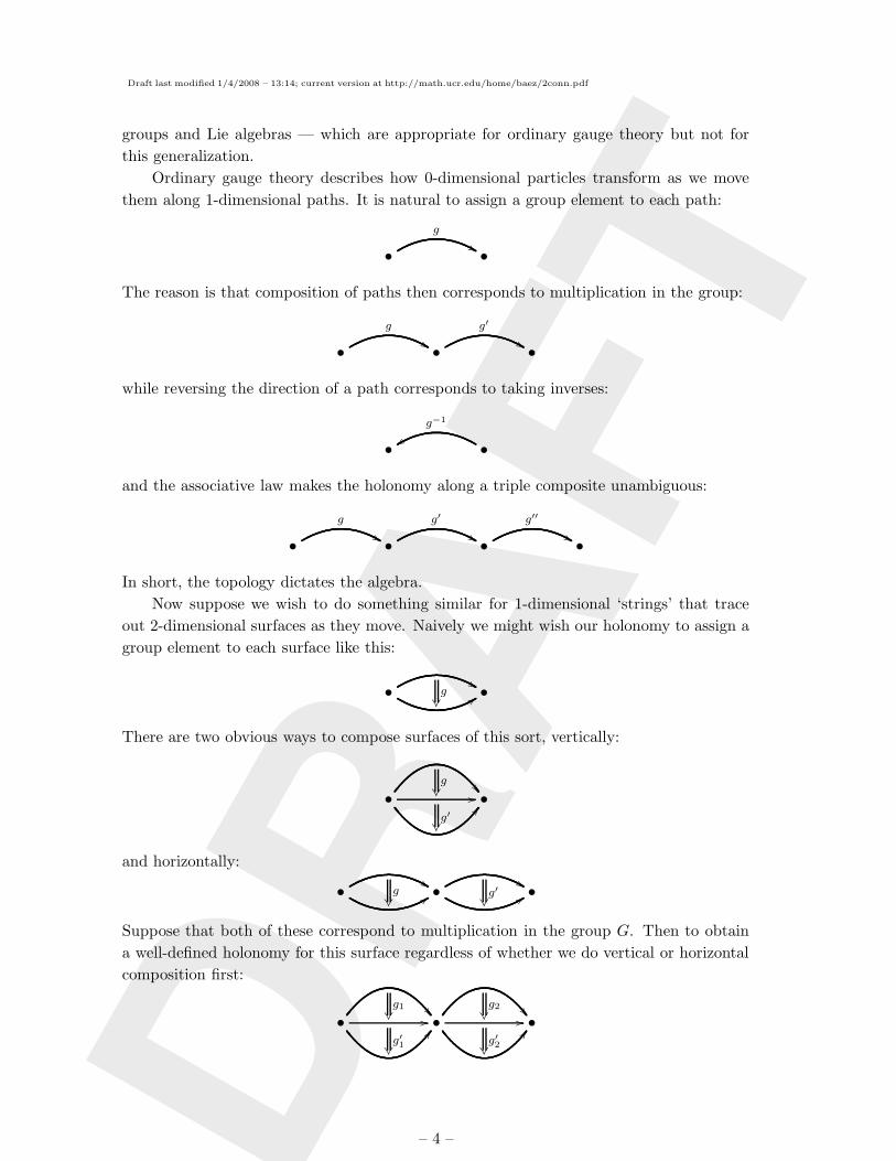
Ordinary gauge theory describes how 0-dimensional particles transform as we move
them along 1-dimensional paths. It is natural to assign a group element to each path:
•g
%% •
The reason is that composition of paths then corresponds to multiplication in the group:
•g
%% •g′
%% •
while reversing the direction of a path corresponds to taking inverses:
• •g−1
yy
and the associative law makes the holonomy along a triple composite unambiguous:
•g
%% •g′
%% •g′′
%% •
In short, the topology dictates the algebra.
Now suppose we wish to do something similar for 1-dimensional ‘strings’ that trace
out 2-dimensional surfaces as they move. Naively we might wish our holonomy to assign a
group element to each surface like this:
• %%99g
•
There are two obvious ways to compose surfaces of this sort, vertically:
• //
g
CCg′
•
and horizontally:
• %%99g
• %%
99g′
•
Suppose that both of these correspond to multiplication in the group G. Then to obtain
a well-defined holonomy for this surface regardless of whether we do vertical or horizontal
composition first:
• //
g1
CCg′1
• //
g2
CCg′2
•
– 4 –
Draft last modified 1/4/2008 – 13:14; current version at http://math.ucr.edu/home/baez/2conn.pdf
DR
AFT
we must have
(g1g2)(g′1g′2) = (g1g
′1)(g2g
′2).
This forces G to be abelian!
In fact, this argument goes back to a classic paper by Eckmann and Hilton [21]. More-
over, they showed that even if we allow G to be equipped with two products, say g g ′ for
vertical composition and gg′ for horizontal, so long as both products share the same unit
and satisfy this ‘interchange law’:
(g1 g′1)(g2 g′2) = (g1g2) (g′1g′2)
then in fact they must agree — so by the previous argument, both are abelian. The proof
is very easy:
gg′ = (g 1)(1 g′) = (g1) (1g′) = g g′.Pursuing this approach, we would ultimately reach the theory of connections on
‘abelian gerbes’. If G = U(1), such a connections looks locally like a 2-form — and it
shows up naturally in string theory, satisfying equations very much like those of electro-
magnetism.
To go beyond this and obtain nonabelian higher gauge fields, we must let the topology
dictate the algebra. Readers familiar with higher categories will already have noticed that
1-dimensional pictures above resemble diagrams in category theory, while the 2-dimensional
pictures resemble diagrams in 2-category theory. This suggests that instead of a Lie group,
the holonomies in higher gauge theory should take values in some sort of categorified
analogue, which we could call a ‘Lie 2-group’.
In fact, even without knowing about higher categories, we can be led to the definition
of a Lie 2-group by considering a kind of connection that gives holonomies both for paths
and for surfaces.
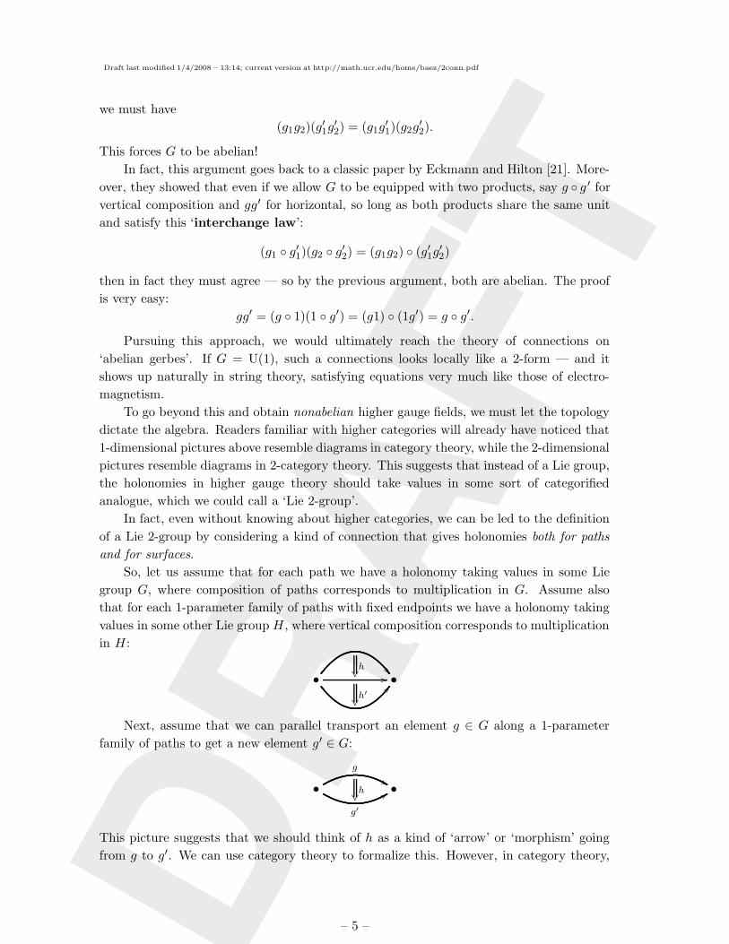
So, let us assume that for each path we have a holonomy taking values in some Lie
group G, where composition of paths corresponds to multiplication in G. Assume also
that for each 1-parameter family of paths with fixed endpoints we have a holonomy taking
values in some other Lie group H, where vertical composition corresponds to multiplication
in H:
• //
h
CCh′
•
Next, assume that we can parallel transport an element g ∈ G along a 1-parameter
family of paths to get a new element g ′ ∈ G:
•g
%%
g′
99h
•
This picture suggests that we should think of h as a kind of ‘arrow’ or ‘morphism’ going
from g to g′. We can use category theory to formalize this. However, in category theory,
– 5 –
Draft last modified 1/4/2008 – 13:14; current version at http://math.ucr.edu/home/baez/2conn.pdf
DR
AFT
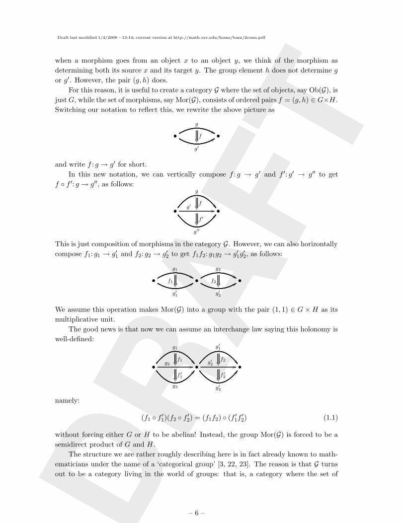
when a morphism goes from an object x to an object y, we think of the morphism as
determining both its source x and its target y. The group element h does not determine g
or g′. However, the pair (g, h) does.
For this reason, it is useful to create a category G where the set of objects, say Ob(G), is
justG, while the set of morphisms, say Mor(G), consists of ordered pairs f = (g, h) ∈ G×H.
Switching our notation to reflect this, we rewrite the above picture as
•g
%%
g′
99f
•
and write f : g → g′ for short.
In this new notation, we can vertically compose f : g → g ′ and f ′: g′ → g′′ to get
f f ′: g → g′′, as follows:
•
g
g′ //f
g′′
CCf ′
•
This is just composition of morphisms in the category G. However, we can also horizontally
compose f1: g1 → g′1 and f2: g2 → g′2 to get f1f2: g1g2 → g′1g′2, as follows:
•g1
%%
g′1
99f1
•g2
%%
g′2
99f2
•
We assume this operation makes Mor(G) into a group with the pair (1, 1) ∈ G ×H as its
multiplicative unit.
The good news is that now we can assume an interchange law saying this holonomy is
well-defined:
•
g1
g2 //f1
g3
CCf ′1
•
g′1
g′2 //f2
g′3
CCf ′2
•
namely:
(f1 f ′1)(f2 f ′2) = (f1f2) (f ′1f′2) (1.1)
without forcing either G or H to be abelian! Instead, the group Mor(G) is forced to be a
semidirect product of G and H.
The structure we are rather roughly describing here is in fact already known to math-
ematicians under the name of a ‘categorical group’ [3, 22, 23]. The reason is that G turns
out to be a category living in the world of groups: that is, a category where the set of
– 6 –
Draft last modified 1/4/2008 – 13:14; current version at http://math.ucr.edu/home/baez/2conn.pdf
DR
AFT
objects is a group, the set of morphisms is a group, and all the usual category operations
are group homomorphisms. To keep the terminology succinct and to hint at generalizations
to still higher-dimensional holonomies, we prefer to call this sort of structure a ‘2-group’.
Moreover, we shall focus our attention on ‘Lie 2-groups’, where the objects and morphisms
form Lie groups, and all the operations are smooth.
In fact, one can develop a full-fledged theory of bundles, connections, curvature, and so
on with a Lie 2-group taking the place of a Lie group. To do this, one must systematically
engage in a process of ‘categorification’, replacing set-based concepts by their category-
based analogues. For example, just as 2-groups are categorified groups, we can define ‘Lie
2-algebras’, which are categorified Lie algebras [4].
So far most work on categorified gauge theory has focused on the special case when
G is trivial and H = U(1), using the language of ‘U(1) gerbes’ [18, 24, 25, 26, 27, 28].
Here, however, we really want H to be nonabelian, and for this we need G to be nontrivial.
Some important progress in this direction can be found in Breen and Messing’s paper on
the differential geometry of ‘nonabelian gerbes’ [13]. While they use different terminology,
their work basically develops the theory of connections and curvature for Lie 2-groups
where H is an arbitrary Lie group, G = Aut(H) is its group of automorphisms, t sends
each element of H to the corresponding inner automorphism, and the action of G on H
is the obvious one. We call this sort of Lie 2-group the ‘automorphism 2-group’ of H.
Luckily, it is easy to extrapolate the whole theory from this case.
In particular, for any Lie 2-group G one can define the notion of a ‘principal 2-bundle’
having G as its gauge 2-group; this has recently been done by Bartels [6]. The first goal of
this paper is to define a concept of ‘2-connection’ for these principal 2-bundles The second
is to show that given a 2-connection, one can define holonomies for paths and surfaces
which behave just as one would hope:
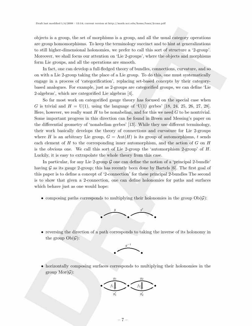
• composing paths corresponds to multiplying their holonomies in the group Ob(G):
•g
%% •g′
%% •
• reversing the direction of a path corresponds to taking the inverse of its holonomy in
the group Ob(G):
• •g−1
yy
• horizontally composing surfaces corresponds to multiplying their holonomies in the
group Mor(G):
•g1
%%
g′1
99f1
•g2
%%
g′2
99f2
•
– 7 –
Draft last modified 1/4/2008 – 13:14; current version at http://math.ucr.edu/home/baez/2conn.pdf
DR
AFT
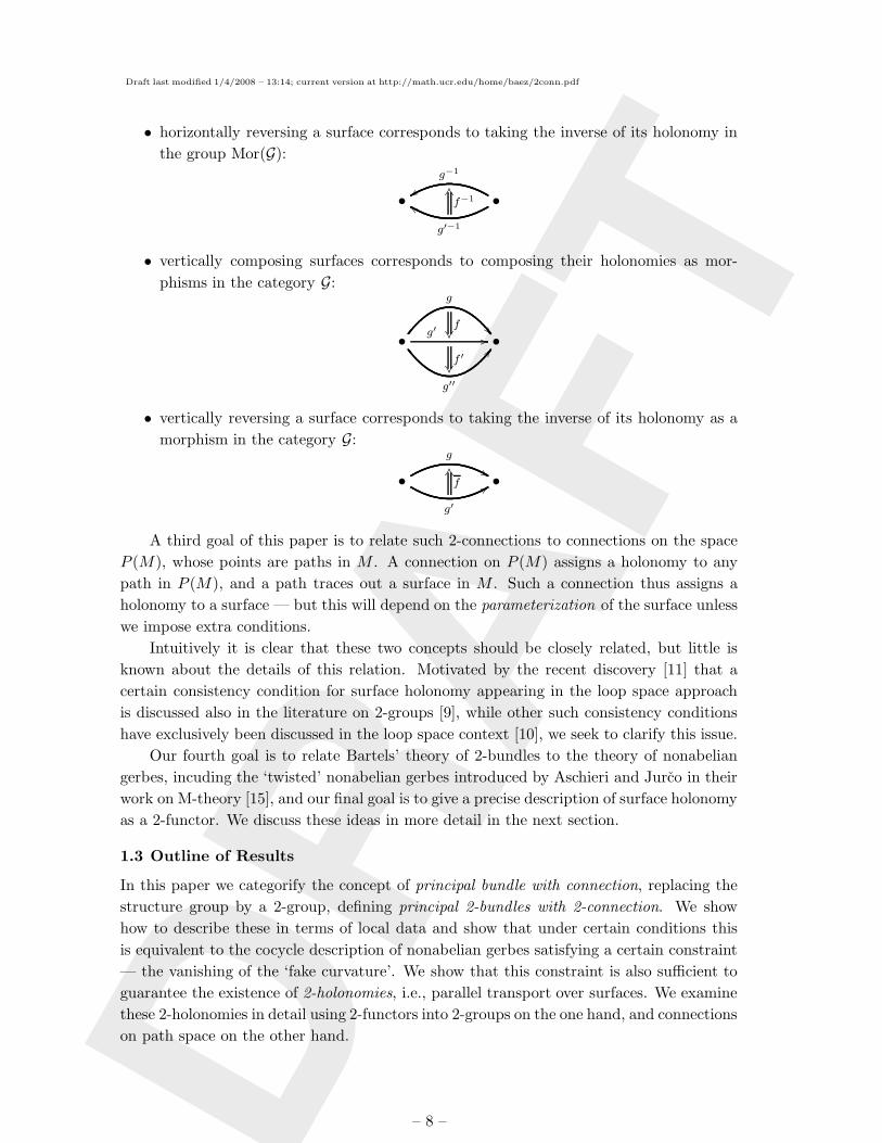
• horizontally reversing a surface corresponds to taking the inverse of its holonomy in
the group Mor(G):
• •g′−1
ee
g−1
yyf−1
KS
• vertically composing surfaces corresponds to composing their holonomies as mor-
phisms in the category G:
•
g
g′ //f
g′′
CCf ′
•
• vertically reversing a surface corresponds to taking the inverse of its holonomy as a
morphism in the category G:
•g
%%
g′
99f
KS•
A third goal of this paper is to relate such 2-connections to connections on the space
P (M), whose points are paths in M . A connection on P (M) assigns a holonomy to any
path in P (M), and a path traces out a surface in M . Such a connection thus assigns a
holonomy to a surface — but this will depend on the parameterization of the surface unless
we impose extra conditions.
Intuitively it is clear that these two concepts should be closely related, but little is
known about the details of this relation. Motivated by the recent discovery [11] that a
certain consistency condition for surface holonomy appearing in the loop space approach
is discussed also in the literature on 2-groups [9], while other such consistency conditions
have exclusively been discussed in the loop space context [10], we seek to clarify this issue.
Our fourth goal is to relate Bartels’ theory of 2-bundles to the theory of nonabelian
gerbes, incuding the ‘twisted’ nonabelian gerbes introduced by Aschieri and Jurco in their
work on M-theory [15], and our final goal is to give a precise description of surface holonomy
as a 2-functor. We discuss these ideas in more detail in the next section.
1.3 Outline of Results
In this paper we categorify the concept of principal bundle with connection, replacing the
structure group by a 2-group, defining principal 2-bundles with 2-connection. We show
how to describe these in terms of local data and show that under certain conditions this
is equivalent to the cocycle description of nonabelian gerbes satisfying a certain constraint
— the vanishing of the ‘fake curvature’. We show that this constraint is also sufficient to
guarantee the existence of 2-holonomies, i.e., parallel transport over surfaces. We examine
these 2-holonomies in detail using 2-functors into 2-groups on the one hand, and connections
on path space on the other hand.
– 8 –
Draft last modified 1/4/2008 – 13:14; current version at http://math.ucr.edu/home/baez/2conn.pdf
DR
AFT
Several aspects of this have been studied before. Categorification is described in [1]
and its application to groups and Lie algebras, which yields 2-groups and Lie 2-algebras, is
discussed in [3, 4, 2]. The concept of 2-group was incorporated in the definition of principal
2-bundles (without connection) in [6]. A description of 2-connections as 2-functors was
introduced in [7, 8, 9], but only in a discretized context, which makes it a bit tricky to treat
global issues. Connections on path space were discussed in [10, 11], and reparametrization
invariance for a special case was investigated by [12]. Cocycle data for nonabelian gerbes
with connection and curving were obtained first by Breen and Messing [13] using algebraic
geometry, and later by Aschieri and Jurco [14, 15] using a nonabelian generalization of
bundle gerbes [16].
Here we extend this work by:
• defining the concept of a principal 2-bundle with 2-connection,
• showing that a 2-connection on a trivial principal 2-bundle has 2-holonomies defining
a 2-functor into the structure 2-group when the 2-connection has vanishing ‘fake
curvature’ (a concept already defined for nonabelian gerbes by Breen and Messing
[13]),
• clarifying the relation between connections on a trivial principal bundle over the
path space of a manifold and 2-connections on a trivial principal 2-bundle over the
manifold itself, showing that a connection on the path space whose holonomies are
invariant under arbitrary surface reparameterizations defines a 2-connection on the
original manifold,
• deriving the local ‘gluing data’ that describe how a nontrivial 2-bundle with 2-
connection can be built from trivial 2-bundles with 2-connection on open sets that
cover the base manifold,
• demonstrating that these gluing data for 2-bundles with 2-connection coincide with
the cocycle description of nonabelian gerbes, subject to the constraint of vanishing
fake curvature.
The starting point for all these considerations is the ordinary concept of a principal
fiber bundle. Such a bundle can be specified using the following ‘gluing data’:
• a base manifold M ,
• a cover of M by open sets Uii∈I ,
• a Lie group G (the ‘gauge group’ or ‘structure group’),
• on each double overlap Uij = Ui ∩ Uj a G-valued function gij ,
• such that on triple overlaps the following transition law holds:
gijgjk = gik.
– 9 –
Draft last modified 1/4/2008 – 13:14; current version at http://math.ucr.edu/home/baez/2conn.pdf
DR
AFT
Such a bundle is augmented with a connection by specifying:
• in each open set Ui a smooth functor holi:P1(Ui)→ G from the path groupoid of Uito the gauge group,
• such that for all paths γ in double overlaps Uij the following transition law holds:
holi(γ) = gij holj(γ) g−1ij .
Here the ‘path groupoid’ P1(M) of a manifold M has points of M as objects and certain
equivalence classes of smooth paths in M as morphisms. There are various ways to work out
the technical details and make P1(M) into a ‘smooth groupoid’; see [18] for the approach
we adopt, which uses ‘thin homotopy classes’ of smooth paths. Technical details aside, the
basic idea is that a connection on a trivial G-bundle gives a well-behaved map assigning
to each path γ in the base space the holonomy hol(γ) ∈ G of the connection along that
path. Saying this map is a ‘smooth functor’ means that these holonomies compose when
we compose paths, and that the holonomy hol(γ) depends smoothly on the path γ.
Our task shall be to categorify all of this and to work out the consequences. The basic
tool will be internalization: given a mathematical concept X defined solely in terms of
sets, functions and commutative diagrams involving these, and given some category K, one
obtains the concept of an ‘X in K’ by replacing all these sets, functions and commutative
diagrams by corresponding objects, morphisms, and commutative diagrams in K.
For example, take X to be the concept of ‘group’. A group in Diff (the category with
smooth manifolds as objects and smooth maps as morphisms) is nothing but a Lie group.
In other words, a Lie group is a group that is a manifold, for which all the group operations
are smooth maps. Similarly, a group in Top (the category with topological spaces as objects
and continuous maps as morphisms) is a topological group.
These examples are standard, but we will need some slightly less familiar ones. In
particular, we will need the concept of ‘2-group’, which is a group in Cat (the category
with categories as objects and functors as morphisms). By a charming principle called
‘commutativity of internalization’, 2-groups can also be thought of as categories in Grp (the
category with groups as objects and homomorphisms as morphisms). We will also need
the concept of a ‘2-space’, which is a category in Diff, or more generally in some category
of smooth spaces that allows for infinite-dimensional examples. A specially nice sort of
2-space is a ‘smooth groupoid’, a concept already mentioned above without explanation:
this is a groupoid in the category of smooth spaces. Finally, a ‘Lie 2-group’ is a 2-group in
Diff.
To arrive at the definition of a 2-bundle E → M , the first steps are to replace the
total space E and base space M by 2-spaces, and to replace the structure group by a Lie
2-group. In this paper we will actually keep the base space an ordinary space, which can be
regarded as a 2-space with only identity morphisms. This is sufficiently general for many
purposes. However, for applications to string theory we may ultimately need 2-bundles
where the base space has points in some manifold as objects and paths or loops in this
manifold as morphisms [19]. This sort of application also requires that we consider smooth
spaces that are more general than finite-dimensional manifolds.
– 10 –
Draft last modified 1/4/2008 – 13:14; current version at http://math.ucr.edu/home/baez/2conn.pdf
DR
AFT
Just as a connection on a trivial principal bundle over M gives a functor hol from
the path groupoid of M to the structure group, one might hope that a 2-connection on a
trivial principal 2-bundle would define a 2-functor from some sort of ‘path 2-groupoid’ to
the structure 2-group. This has already been studied in the context of higher lattice gauge
theory [8, 9]. Thus, the main issues not yet addressed are those involving differentiability.
To address these issues, we define for any smooth space M a smooth 2-groupoid P2(M)
such that:
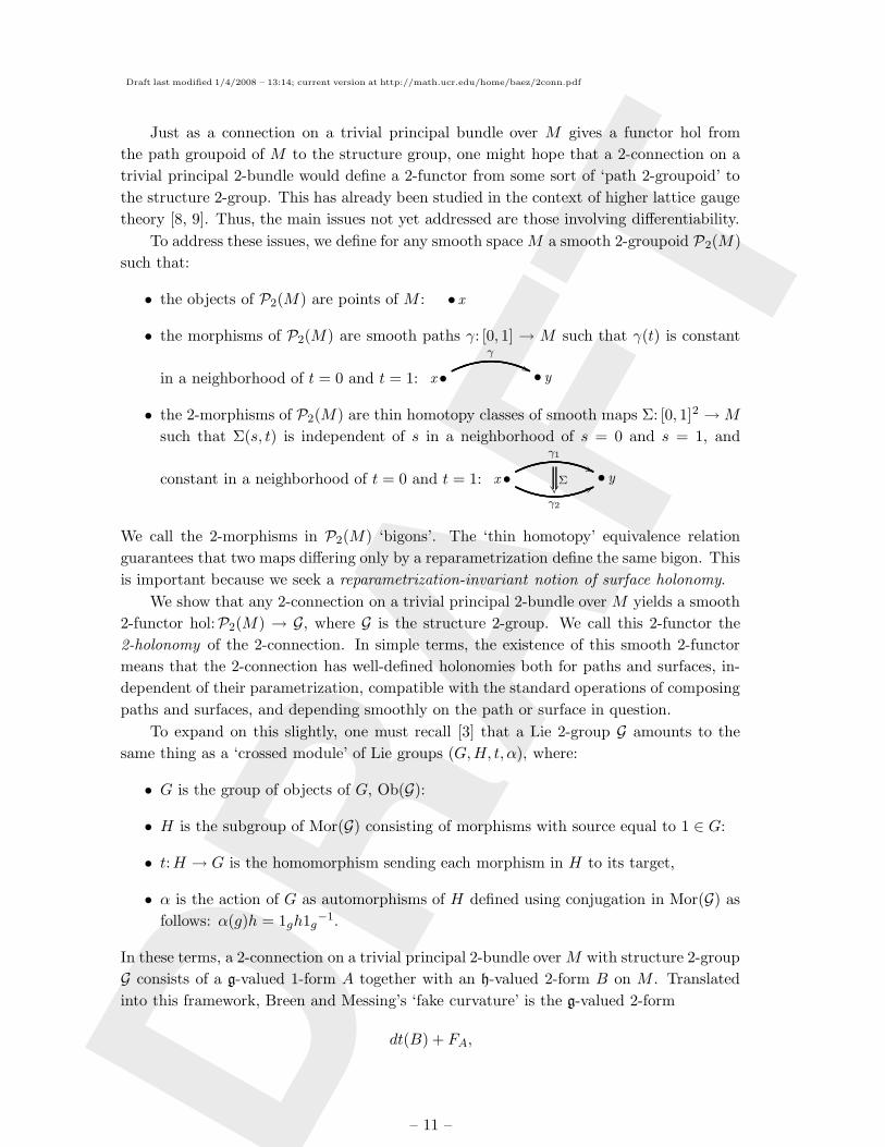
• the objects of P2(M) are points of M : • x
• the morphisms of P2(M) are smooth paths γ: [0, 1] → M such that γ(t) is constant
in a neighborhood of t = 0 and t = 1: x •γ
'' • y
• the 2-morphisms of P2(M) are thin homotopy classes of smooth maps Σ: [0, 1]2 →M
such that Σ(s, t) is independent of s in a neighborhood of s = 0 and s = 1, and
constant in a neighborhood of t = 0 and t = 1: x •γ1
''
γ2
77 • yΣ
We call the 2-morphisms in P2(M) ‘bigons’. The ‘thin homotopy’ equivalence relation
guarantees that two maps differing only by a reparametrization define the same bigon. This
is important because we seek a reparametrization-invariant notion of surface holonomy.
We show that any 2-connection on a trivial principal 2-bundle over M yields a smooth
2-functor hol:P2(M) → G, where G is the structure 2-group. We call this 2-functor the
2-holonomy of the 2-connection. In simple terms, the existence of this smooth 2-functor
means that the 2-connection has well-defined holonomies both for paths and surfaces, in-
dependent of their parametrization, compatible with the standard operations of composing
paths and surfaces, and depending smoothly on the path or surface in question.
To expand on this slightly, one must recall [3] that a Lie 2-group G amounts to the
same thing as a ‘crossed module’ of Lie groups (G,H, t, α), where:
• G is the group of objects of G, Ob(G):
• H is the subgroup of Mor(G) consisting of morphisms with source equal to 1 ∈ G:
• t:H → G is the homomorphism sending each morphism in H to its target,
• α is the action of G as automorphisms of H defined using conjugation in Mor(G) as
follows: α(g)h = 1gh1g−1.
In these terms, a 2-connection on a trivial principal 2-bundle over M with structure 2-group
G consists of a g-valued 1-form A together with an h-valued 2-form B on M . Translated
into this framework, Breen and Messing’s ‘fake curvature’ is the g-valued 2-form
dt(B) + FA,
– 11 –
Draft last modified 1/4/2008 – 13:14; current version at http://math.ucr.edu/home/baez/2conn.pdf
DR
AFT
where FA = dA+A ∧ A is the usual curvature of A. We show that if and only if the fake
curvature vanishes, there is a well-defined 2-holonomy hol:P2(M)→ G.
The importance of vanishing fake curvature in the framework of lattice gauge theory
was already emphasized in [9]. The special case where also FA = 0 was studied in [10],
while a discussion of this constraint in terms of loop space in the case G = H was given in
[11]. Our result subsumes these cases in a common framework.
This framework for 2-connections on trivial 2-bundles is sufficient for local considera-
tions. Thus, all that remains is to turn it into a global notion by categorifying the transition
laws for a principal bundle with connection, which in terms of local data read:
gijgjk = gik
holi(γ) = gij holj(γ) g−1ij .
The basic idea is to replace these equations by specified isomorphisms, using the fact that a
2-group G has not only objects (forming the group G) but also morphisms (described with
the help of the group H). These isomorphisms should in turn satisfy certain coherence
laws of their own. These coherence laws have already been worked out for 2-bundles
without connection [6] and for twisted nonabelian gerbes with connection and curving
[13, 14, 15]; here we put these ideas together. We show that the local data describing such
2-bundles with 2-connection matches the cocycle data describing nonabelian bundle gerbes
with connection and curving, subject to the constraint of vanishing fake curvature.
In summary, we find that categorifying the notion of a principal bundle with connection
gives a structure that includes as a special case nonabelian bundle gerbes with connection
and curving, with vanishing fake curvature.
1.4 Structure of the Paper
We begin in §2 with a review of internalization, Lie 2-groups and Lie 2-algebras, and
nonabelian gerbes. This prepares us to explain 2-bundles in §3, and to show how they can
be described using local gluing data.
After 2-bundles have been described in this way, we define the concept of 2-connection
in §4. Here we also state our main result, Theorem 39, which describes 2-connections in
terms of Lie-algebra-valued differential forms. We begin the proof of this result in §5.
Finally, in §6 we relate 2-connections on a manifold to connections on its path space, and
use this to conclude the proof.
– 12 –
Draft last modified 1/4/2008 – 13:14; current version at http://math.ucr.edu/home/baez/2conn.pdf
DR
AFT
2. Preliminaries
To develop the theory of 2-connections on 2-bundles, we need some mathematical prelim-
inaries on internalization (§2.1), with special emphasis on 2-spaces (§2.2), Lie 2-groups
(§2.3), and Lie 2-algebras (§2.4). We also review the theory of nonabelian gerbes (§2.5).
2.1 Internalization
To categorify concepts from differential geometry, we will use a procedure called ‘inter-
nalization’. Developed by Lawvere [29], Ehresmann [30] and others, internalization is a
method for generalizing concepts from ordinary set-based mathematics to other contexts
— or more precisely, to other categories. This method is simple and elegant. To internalize
a concept, we merely have to describe it using commutative diagrams in the category of
sets, and then interpret these diagrams in some other category K. For example, if we in-
ternalize the concept of ‘group’ in the category of topological spaces, we obtain the concept
of ‘topological group’.
For categorification, the main concept we need to internalize is that of a category
itself! To do this, we start by writing down the definition of category using commutative
diagrams. We do this in terms of the functions s and t assigning to any morphism f :x→ y
its source and target:
s(f) = x, t(f) = y,
the function i assigning to any object its identity morphism:
i(x) = 1x,
and the function assigning to any composable pair of morphisms their composite:
(f, g) = f g
If we write Ob(C) for the set of objects and Mor(C) for the set of morphisms of a category
C, the set of composable pairs of morphisms is denoted Mor(C)t×sMor(C), since it consists
of pairs (f, g) with t(f) = s(g).
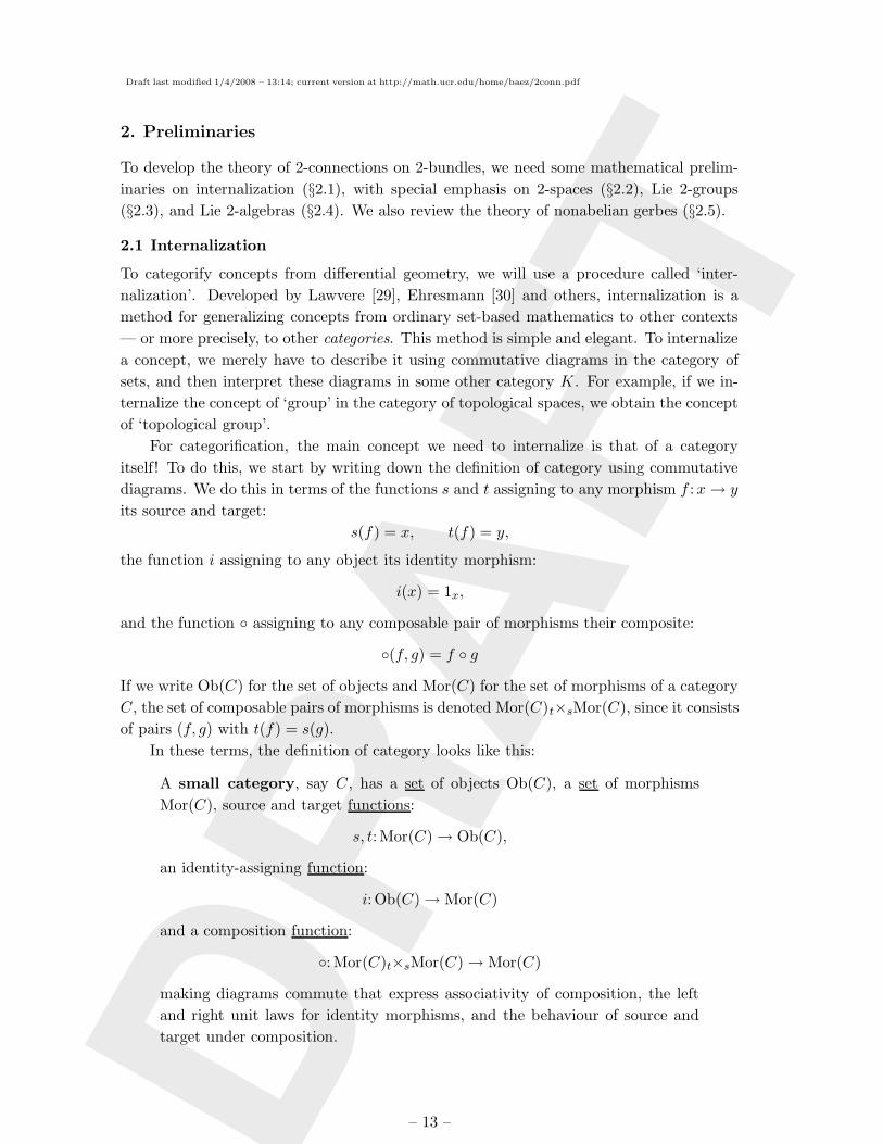
In these terms, the definition of category looks like this:
A small category, say C, has a set of objects Ob(C), a set of morphisms
Mor(C), source and target functions:
s, t: Mor(C)→ Ob(C),
an identity-assigning function:
i: Ob(C)→ Mor(C)
and a composition function:
: Mor(C)t×sMor(C)→ Mor(C)
making diagrams commute that express associativity of composition, the left
and right unit laws for identity morphisms, and the behaviour of source and
target under composition.
– 13 –
Draft last modified 1/4/2008 – 13:14; current version at http://math.ucr.edu/home/baez/2conn.pdf
DR
AFT
We omit the actual diagrams because they are not very enlightening: the reader can find
them elsewhere [4, 31] or reinvent them. The main point here is not so much what they
are, as that they can be written down.
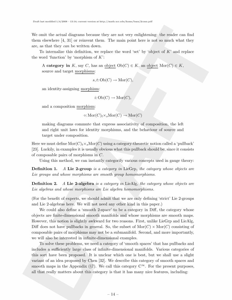
To internalize this definition, we replace the word ‘set’ by ‘object of K’ and replace
the word ‘function’ by ‘morphism of K’:
A category in K, say C, has an object Ob(C) ∈ K, an object Mor(C) ∈ K,
source and target morphisms:
s, t: Ob(C)→ Mor(C),
an identity-assigning morphism:
i: Ob(C)→ Mor(C),
and a composition morphism:
: Mor(C)t×sMor(C)→ Mor(C)
making diagrams commute that express associativity of composition, the left
and right unit laws for identity morphisms, and the behaviour of source and
target under composition.
Here we must define Mor(C)t×sMor(C) using a category-theoretic notion called a ‘pullback’
[23]. Luckily, in examples it is usually obvious what this pullback should be, since it consists
of composable pairs of morphisms in C.
Using this method, we can instantly categorify various concepts used in gauge theory:
Definition 1. A Lie 2-group is a category in LieGrp, the category whose objects are
Lie groups and whose morphisms are smooth group homomorphisms.
Definition 2. A Lie 2-algebra is a category in LieAlg, the category whose objects are
Lie algebras and whose morphisms are Lie algebra homomorphisms.
(For the benefit of experts, we should admit that we are only defining ‘strict’ Lie 2-groups
and Lie 2-algebras here. We will not need any other kind in this paper.)
We could also define a ‘smooth 2-space’ to be a category in Diff, the category whose
objects are finite-dimensional smooth manifolds and whose morphisms are smooth maps.
However, this notion is slightly awkward for two reasons. First, unlike LieGrp and LieAlg,
Diff does not have pullbacks in general. So, the subset of Mor(C)×Mor(C) consisting of
composable pairs of morphisms may not be a submanifold. Second, and more importantly,
we will also be interested in infinite-dimensional examples.
To solve these problems, we need a category of ‘smooth spaces’ that has pullbacks and
includes a sufficiently large class of infinite-dimensional manifolds. Various categories of
this sort have been proposed. It is unclear which one is best, but we shall use a slight
variant of an idea proposed by Chen [32]. We describe this category of smooth spaces and
smooth maps in the Appendix (§7). We call this category C∞. For the present purposes,
all that really matters about this category is that it has many nice features, including:
– 14 –
Draft last modified 1/4/2008 – 13:14; current version at http://math.ucr.edu/home/baez/2conn.pdf
DR
AFT
• Every finite-dimensional smooth manifold (possibly with boundary) is a smooth
space, with smooth maps between these being precisely those that are smooth in
the usual sense.
• Every smooth space has a topology, and all smooth maps between smooth spaces are
continuous.
• Every subset of a smooth space is a smooth space.
• We can form a ‘quotient’ of a smooth space X by any equivalence relation, which is
again smooth space.
• If Xαα∈A are smooth spaces, so is their product∏α∈AXα.
• If Xαα∈A are smooth spaces, so is their disjoint union∐α∈AXα.
• If X and Y are smooth spaces, so is the set C∞(X,Y ) consisting of smooth maps
from X to Y .
• There is an isomorphism of smooth spaces
C∞(A×X,Y ) ∼= C∞(A,C∞(X,Y ))
sending any function φ:A×X → Y to the function φ:A→ C∞(X,Y ) given by
φ(x)(a) = φ(x, a).
• We can define vector fields and differential forms on smooth spaces, with many of
the usual properties.
With the notion of smooth space in hand, we can make the following definition:
Definition 3. A (smooth) 2-space is a category in C∞, the category whose objects are
smooth spaces and whose morphisms are smooth maps.
Not only can we categorify Lie groups, Lie algebras and smooth spaces, we can also
categorify the maps between them. The right sort of map between categories is a functor:
a pair of functions sending objects to objects and morphisms to morphisms, preserving
source, target, identities and composition. If we internalize this concept, we get the defi-
nition of a ‘functor in K’. We then say:
Definition 4. A homomorphism between Lie 2-groups is a functor in LieGrp.
Definition 5. A homomorphism between Lie 2-algebras is a functor in LieAlg.
Definition 6. A (smooth) map between 2-spaces is a functor in C∞.
There are also natural transformations between functors, and internalizing this notion
we can make the following definitions:
– 15 –
Draft last modified 1/4/2008 – 13:14; current version at http://math.ucr.edu/home/baez/2conn.pdf
DR
AFT
Definition 7. A 2-homomorphism between homomorphisms between Lie 2-groups is a
natural transformation in LieGrp.
Definition 8. A 2-homomorphism between homomorphisms between Lie 2-algebras is
a natural transformation in LieAlg.
Definition 9. A (smooth) 2-map between maps between 2-spaces is a natural transfor-
mation in C∞.
Writing down these definitions is quick and easy. It takes longer to understand them
and apply them to higher gauge theory. For this we must unpack them and look at
examples. We do this in the next two sections.
2.2 2-Spaces
Unraveling Def. 3, a smooth 2-space, or 2-space for short, is a category X where:
• The set of objects, Ob(X), is a smooth space.
• The set of morphisms, Mor(X), is a smooth space.
• The functions mapping any morphism to its source and target, s, t: Mor(X) →Ob(X), are smooth maps.
• The function mapping any object to its identity morphism, i: Ob(X) → Mor(X), is
a smooth map
• The function mapping any composable pair of morphisms to their composite,
: Mor(X)s×tMor(X)→ Mor(X), is a smooth map.
2-spaces are more common than one might at first guess. One just needs to know where to
look. First of all, every ordinary smooth space is a 2-space with only identity morphisms.
More interesting examples arise naturally in string theory: the path groupoid and the loop
groupoid of a manifold. In the next section we consider another large class of examples:
Lie 2-groups.
Definition 10. A 2-space with only identity morphisms is called trivial.
Example 11. Any smooth space M gives a trivial 2-space X with Ob(X) = M . This
2-space has Mor(X) = M , with s, t, i, all being the identity map from M to itself. Every
trivial 2-space is of this form.
Example 12. Given a smooth space M , there is a smooth 2-space P1(M), the path
groupoid of M , such that:
• the objects of P1(M) are points of M ,
• the morphisms of P1(M) are thin homotopy classes of smooth paths γ: [0, 1] → M
such that γ(t) is constant near t = 0 and t = 1.
– 16 –
Draft last modified 1/4/2008 – 13:14; current version at http://math.ucr.edu/home/baez/2conn.pdf
DR
AFT
Here a thin homotopy between smooth paths γ0, γ1: [0, 1]→M is a smooth map F : [0, 1]2 →M such that:
• F (0, t) = γ0(t) and F (1, t) = γ1(t),
• F (s, t) is constant for t near 0 and constant for t near 1,
• F (s, t) is independent of s for s near 0 and for s near 1,
• the rank of the differential dF (s, t) is < 2 for all (s, t) ∈ [0, 1]2.
The last condition is what makes the homotopy ‘thin’: it guarantees that the homotopy
sweeps out a surface of vanishing area.
To see how P1(M) becomes a 2-space, first note that the space of smooth maps
γ: [0, 1] → M becomes a smooth space in a natural way, as does the subspace satisfying
the constancy conditions near t = 0, 1, and finally the quotient of this subspace consisting
of thin homotopy classes. This makes Mor(P1(M)) into a smooth space. For short, we call
this smooth space P (M), the path space of M . Ob(P1(M)) = M is obviously a smooth
space as well. The source and target maps
s, t: Mor(P1(M))→ Ob(P1(M))
send any equivalence class of paths to its endpoints:
s([γ]) = γ(0), t([γ]) = γ(1).
The identity-assigning map sends any point x ∈M to the constant path at this point. The
composition map sends any composable pair of morphisms [γ], [γ ′] to [γ γ′], where
γ γ′(t) =
γ(2t) if 0 ≤ t ≤ 1
2
γ′(2t− 1) if 12 ≤ t ≤ 1
One can check that γ γ ′ is a smooth path and that [γ γ ′] is well-defined and independent
of the choice of representatives for [γ] and [γ ′]. One can also check that the maps s, t, i, are smooth and that the usual rules of a category hold. It follows that P1(M) is a 2-space.
In fact, P1(M) is not just a category: it is also a groupoid: a category where every
morphism has an inverse. The inverse of [γ] is just [γ], where γ is obtained by reversing
the orientation of the path γ:
γ(t) = γ(1− t).Moreover, the map sending any morphism to its inverse is smooth. Thus P1(M) is a
smooth groupoid: a 2-space where every morphism is invertible and the map sending
every morphism to its inverse is smooth.
Example 13. Given a 2-space X, any subcategory of X becomes a 2-space in its own
right. Here a subcategory is a category Y with Ob(Y ) ⊆ Ob(X) and Mor(Y ) ⊆ Mor(X),
where the source, target, identity-assigning and composition maps of Y are restrictions of
those for X. The reason Y becomes a 2-space is that any subspace of a smooth space
becomes a smooth space in a natural way (see §7) and restrictions of smooth maps to
subspaces are smooth. We call Y a sub-2-space of X.
– 17 –
Draft last modified 1/4/2008 – 13:14; current version at http://math.ucr.edu/home/baez/2conn.pdf
DR
AFT
Example 14. Given a smooth space M , the path groupoid P1(M) has a sub-2-space
LM whose objects are all the points of M and whose morphisms are those equivalence
classes [γ] where γ is a loop: that is, a path with γ(0) = γ(1). We call LM the loop
groupoid of M . Like the path groupoid, the loop groupoid of M is not just a 2-space,
but a smooth groupoid.
For 2-spaces, and indeed for all categorified concepts, the usual notion of ‘isomorphism’
is less useful than that of ‘equivalence’. For example, in categorified gauge theory what
matters is not 2-bundles whose fibers are all isomorphic to some standard fiber, but those
whose fibers are all equivalent to some standard fiber. We recall the concept of equivalence
here:
Definition 15. Given 2-spaces X and Y , an isomorphism f :X → Y is a map equipped
with a map f :Y → X called its inverse such that ff = 1X and f f = 1Y . An equivalence
f :X → Y is a map equipped with a map f :Y → X called its weak inverse together with
invertible 2-maps φ: ff∼
=⇒1X and φ: f f∼
=⇒1Y .
2.3 Lie 2-Groups
Unravelling Def. 1, we see that a Lie 2-group G is a category where:
• The set of objects, Ob(G), is a Lie group.
• The set of morphisms, Mor(G), is a Lie group.
• The functions mapping any morphism to its source and target, s, t: Mor(G)→ Ob(G),
are homomorphisms.
• The function mapping any object to its identity morphism, i: Ob(G)→ Mor(G), is a
homomorphism.
• The function mapping any composable pair of morphisms to their composite,
: Mor(G)s×tMor(G)→ Mor(G), is a homomorphism.
For applications to higher gauge theory it is suggestive to draw objects of G as arrows:
•g
%% •
and morphisms f : g → g′ as surfaces of this sort:
•g
%%
g′
99f
•
This lets us can draw multiplication in Ob(G) as composition of arrows, multiplication in
Mor(G) as ‘horizontal composition’ of surfaces, and composition of morphisms f : g → g ′
and f ′: g′ → g′′ as ‘vertical composition’ of surfaces, as explained in §1.2.
– 18 –
Draft last modified 1/4/2008 – 13:14; current version at http://math.ucr.edu/home/baez/2conn.pdf
DR
AFT
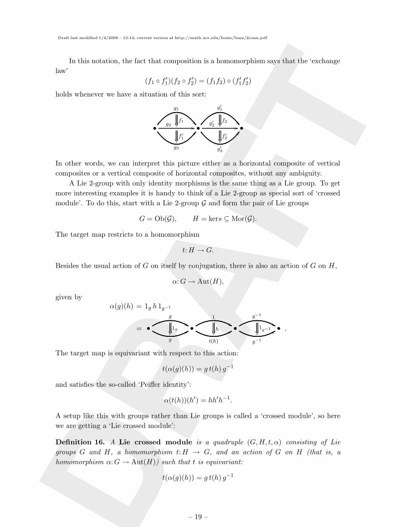
In this notation, the fact that composition is a homomorphism says that the ‘exchange
law’
(f1 f ′1)(f2 f ′2) = (f1f2) (f ′1f′2)
holds whenever we have a situation of this sort:
•
g1
g2 //f1
g3
CCf ′1
•
g′1
g′2 //f2
g′3
CCf ′2
•
In other words, we can interpret this picture either as a horizontal composite of vertical
composites or a vertical composite of horizontal composites, without any ambiguity.
A Lie 2-group with only identity morphisms is the same thing as a Lie group. To get
more interesting examples it is handy to think of a Lie 2-group as special sort of ‘crossed
module’. To do this, start with a Lie 2-group G and form the pair of Lie groups
G = Ob(G), H = kers ⊆ Mor(G).
The target map restricts to a homomorphism
t:H → G.
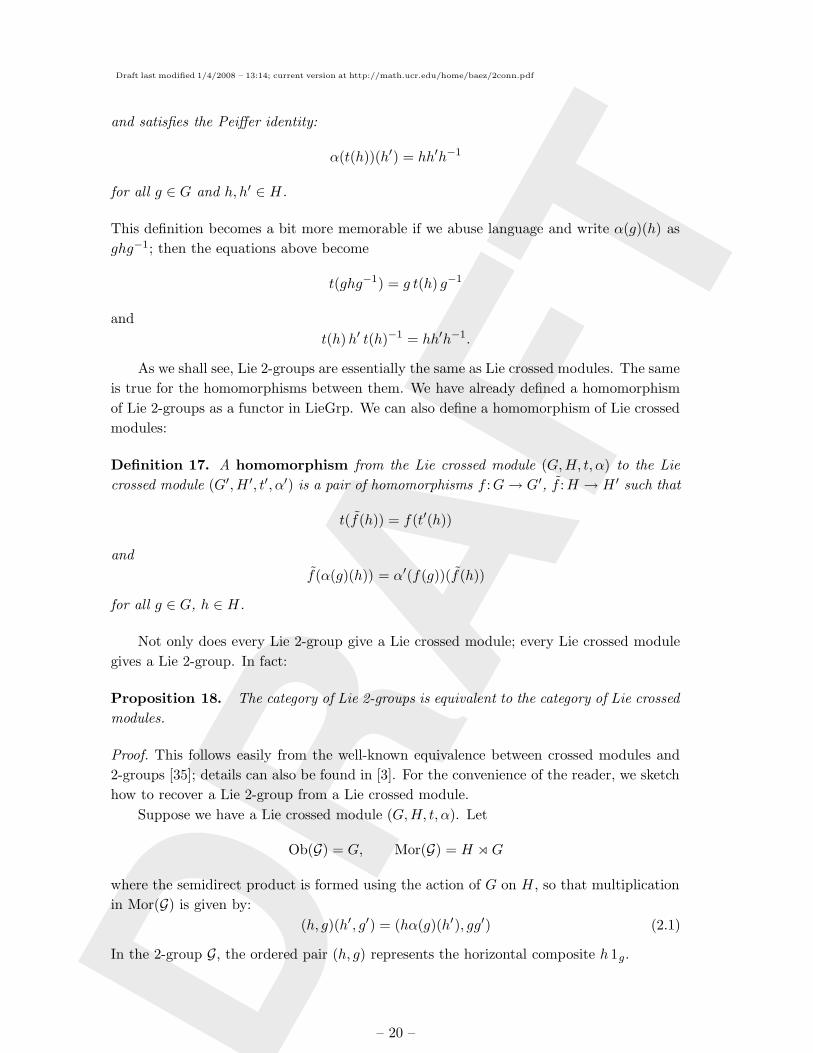
Besides the usual action of G on itself by conjugation, there is also an action of G on H,
α:G→ Aut(H),
given byα(g)(h) = 1g h 1g−1
= •g
%%
g
991g
•1
%%
t(h)
99h
•g−1
%%
g−1
991g−1
• .
The target map is equivariant with respect to this action:
t(α(g)(h)) = g t(h) g−1
and satisfies the so-called ‘Peiffer identity’:
α(t(h))(h′) = hh′h−1.
A setup like this with groups rather than Lie groups is called a ‘crossed module’, so here
we are getting a ‘Lie crossed module’:
Definition 16. A Lie crossed module is a quadruple (G,H, t, α) consisting of Lie
groups G and H, a homomorphism t:H → G, and an action of G on H (that is, a
homomorphism α:G→ Aut(H)) such that t is equivariant:
t(α(g)(h)) = g t(h) g−1
– 19 –
Draft last modified 1/4/2008 – 13:14; current version at http://math.ucr.edu/home/baez/2conn.pdf
DR
AFT
and satisfies the Peiffer identity:
α(t(h))(h′) = hh′h−1
for all g ∈ G and h, h′ ∈ H.
This definition becomes a bit more memorable if we abuse language and write α(g)(h) as
ghg−1; then the equations above become
t(ghg−1) = g t(h) g−1
and
t(h)h′ t(h)−1 = hh′h−1.
As we shall see, Lie 2-groups are essentially the same as Lie crossed modules. The same
is true for the homomorphisms between them. We have already defined a homomorphism
of Lie 2-groups as a functor in LieGrp. We can also define a homomorphism of Lie crossed
modules:
Definition 17. A homomorphism from the Lie crossed module (G,H, t, α) to the Lie
crossed module (G′,H ′, t′, α′) is a pair of homomorphisms f :G→ G′, f :H → H ′ such that
t(f(h)) = f(t′(h))
and
f(α(g)(h)) = α′(f(g))(f (h))
for all g ∈ G, h ∈ H.
Not only does every Lie 2-group give a Lie crossed module; every Lie crossed module
gives a Lie 2-group. In fact:
Proposition 18. The category of Lie 2-groups is equivalent to the category of Lie crossed
modules.
Proof. This follows easily from the well-known equivalence between crossed modules and
2-groups [35]; details can also be found in [3]. For the convenience of the reader, we sketch
how to recover a Lie 2-group from a Lie crossed module.
Suppose we have a Lie crossed module (G,H, t, α). Let
Ob(G) = G, Mor(G) = H oG
where the semidirect product is formed using the action of G on H, so that multiplication
in Mor(G) is given by:
(h, g)(h′, g′) = (hα(g)(h′), gg′) (2.1)
In the 2-group G, the ordered pair (h, g) represents the horizontal composite h 1g.
– 20 –
Draft last modified 1/4/2008 – 13:14; current version at http://math.ucr.edu/home/baez/2conn.pdf
DR
AFT
The inverse of an element of the group Mor(G) is given by:
(h, g)−1 = (α(g−1)(h−1
), g−1) .
We make G into a Lie 2-group where the source and target maps s, t: Mor(G)→ Ob(G) are
given by:
s(h, g) = g, t(h, g) = t(h)g, (2.2)
the identity-assigning map i: Ob(G)→ Mor(G) is given by:
i(g) = (g, 1), (2.3)
and the composite of the morphisms
(h, g): g → g′, (h′, g′): g′ → g′′,
is
(h, g) (h′, g′) = (hh′, g): g → g′′. (2.4)
It is also worth noting that every morphism has an inverse with respect to composition,
which we denote by:
(h, g) :=(h−1, t(h)g
).
One can check that this construction indeed gives a Lie 2-group, and that together with
the previous construction it sets up an equivalence between the categories of Lie 2-groups
and Lie crossed modules. 2
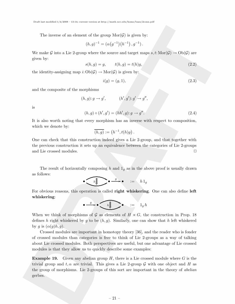
The result of horizontally composing h and 1g as in the above proof is usually drawn
as follows:
• %%99h
• g // • := h 1g
For obvious reasons, this operation is called right whiskering. One can also define left
whiskering:
• g // • %%99h
• := 1g h
When we think of morphisms of G as elements of H o G, the construction in Prop. 18
defines h right whiskered by g to be (h, g). Similarly, one can show that h left whiskered
by g is (α(g)h, g).
Crossed modules are important in homotopy theory [36], and the reader who is fonder
of crossed modules than categories is free to think of Lie 2-groups as a way of talking
about Lie crossed modules. Both perspectives are useful, but one advantage of Lie crossed
modules is that they allow us to quickly describe some examples:
Example 19. Given any abelian group H, there is a Lie crossed module where G is the
trivial group and t, α are trivial. This gives a Lie 2-group G with one object and H as
the group of morphisms. Lie 2-groups of this sort are important in the theory of abelian
gerbes.
– 21 –
Draft last modified 1/4/2008 – 13:14; current version at http://math.ucr.edu/home/baez/2conn.pdf
DR
AFT
Example 20. More generally, given any Lie group G, abelian Lie group H, and action
α of G as automorphisms of H, there is a Lie crossed module with t:G → H the trivial
homomorphism. For example, we can take H to be a finite-dimensional vector space and
α to be a representation of G on this vector space.
In particular, if G is the Lorentz group and α is the defining representation of this
group on Minkowski spacetime, this construction gives a Lie 2-group called the Poincare
2-group, because its group of morphisms is the Poincare group. After its introduction in
work on higher gauge theory [2], this 2-group was used in in some recent work on quantum
gravity by Crane, Sheppeard and Yetter [37, 38].
Example 21. Given any Lie group H, there is a Lie crossed module with G = Aut(H),
t:H → G the homomorphism assigning to each element of H the corresponding inner auto-
morphism, and the obvious action of G as automorphisms of H. We call the corresponding
Lie 2-group the automorphism 2-group of H, and denote it by AUT (H). This sort of
2-group is important in the theory of nonabelian gerbes.
In particular, if we take H to be the multiplicative group of nonzero quaternions,
then G = SU(2) and we obtain a 2-group that plays a basic role in Thompson’s theory of
quaternionic gerbes [39].
We use the term ‘automorphism 2-group’ because AUT (H) really is a 2-group of
symmetries of H. An object of AUT (H) is a symmetry of the group H in the usual sense:
that is, an automorphism f :H → H. On the other hand, a morphism θ: f → f ′ in AUT (H)
is a ‘symmetry between symmetries’: that is, an element h ∈ H that sends f to f ′ in the
following sense: hf(x)h−1 = f ′(x) for all x ∈ H.
Example 22. Suppose that 1 → A → Ht−→G → 1 is a central extension of the Lie
group G by the Lie group H. Then there is a Lie crossed module with this choice of
t:G → H. To construct α we pick any section s, that is, any function s:G → H with
t(s(g)) = g, and define
α(g)h = s(g)hs(g)−1.
Since A lies in the center of H, α independent of the choice of s. We do not need a global
smooth section s to show α(g) depends smoothly on g; it suffices that there exist a local
smooth section in a neighborhood of each g ∈ G.
It is easy to generalize this idea to infinite-dimensional cases if we work not with Lie
groups but smooth groups: that is, groups in the category of smooth spaces. The basic
theory of smooth groups, smooth 2-groups and smooth crossed modules works just like
the finite-dimensional case, but with the category of smooth spaces replacing Diff. In
particular, every smooth group G has a Lie algebra g.
Given a connected and simply-connected compact simple Lie group G, the loop group
ΩG is a smooth group. For each ‘level’ k ∈ Z, this group has a central extension
1→ U(1) → ΩkGt−→ΩG→ 1
as explained by Pressley and Segal [40]. The above diagram lives in the category of smooth
groups, and there exist local smooth sections for t: ΩkG → ΩG, so we obtain a smooth
– 22 –
Draft last modified 1/4/2008 – 13:14; current version at http://math.ucr.edu/home/baez/2conn.pdf
DR
AFT
crossed module (ΩG, ΩkG, t, α) with α given as above. This in turn gives an smooth 2-
group which we call the level-k loop 2-group of G, LkG.
It has recently been shown [41] that LkG fits into an exact sequence of smooth 2-groups:
1→ LkG → PkG−→G→ 1
where the middle term, the level-k path 2-group of G, has very interesting properties.
In particular, when k = ±1, the geometric realization of the nerve of PkG is a topological
group that can also be obtained by killing the 3rd homotopy group of G. When G =
Spin(n), this topological group goes by the name of String(n), since it plays a role in defining
spinors on loop space [42]. The group String(n) also shows up in Stolz and Teichner’s work
on elliptic cohomology, which involves a notion of parallel transport over surfaces [43]. So,
we expect that PkG will be an especially interesting structure 2-group for applications of
2-bundles to string theory.
To define the holonomy of a connection, we need smooth groups with an extra property:
namely, that for every smooth function f : [0, 1] → g there is a unique smooth function
g: [0, 1] → G solving the differential equation
d
dtg(t) = f(t)g(t)
with g(0) = 1. We call such smooth groups exponentiable. Similarly, we call a smooth
2-group exponentiable if its crossed module (G,H, t, α) has both G and H exponentiable.
In particular, every Lie group and thus every Lie 2-group is exponentiable. The smooth
groups ΩG and ΩkG are also exponentiable, as are the 2-groups LkG and PkG. So, for
the convenience of stating theorems in a simple way, we henceforth implicitly assume all
smooth groups and 2-groups under discussion are exponentiable.
2.4 Lie 2-Algebras
Just as Lie groups give rise to Lie algebras, Lie 2-groups give rise to Lie 2-algebras. These
can also be described using a differential version of crossed modules. Recall that a Lie
2-algebra is a category L where:
• The set of objects, Ob(L), is a Lie algebra.
• The set of morphisms, Mor(L), is a Lie algebra.
• The functions mapping any morphism to its source and target, s, t: Mor(L)→ Ob(L),
are Lie algebra homomorphisms,
• The function mapping any object to its identity morphism, i: Ob(L)→ Mor(L), is a
Lie algebra homomorphism.
• The function mapping any composable pair of morphisms to their composite,
: Mor(L)s×tMor(L)→ Mor(L), is a Lie algebra homomorphism.
– 23 –
Draft last modified 1/4/2008 – 13:14; current version at http://math.ucr.edu/home/baez/2conn.pdf
DR
AFT
We can get a Lie 2-algebra by differentiating all the data in a Lie 2-group. Similarly,
we can get a ‘differential crossed module’ by differentiating all the data in a Lie crossed
module:
Definition 23. A differential crossed module is a quadruple C = (g, h, dt, dα) con-
sisting of Lie algebras g, h, a homomorphism dt: h→ g, and an action α of g as derivations
of h (that is, a homomorphism α: g→ Der(h)) satisfying
dt(dα(x)(y)) = [x, dt(y)] (2.5)
and
dα(dt(y))(y′) = [y, y′] (2.6)
for all x ∈ g and y, y′ ∈ h.
This definition becomes easier to remember if we allow ourselves to write dα(x)(y) as [x, y].
Then the fact that dα is an action of g as derivations of h simply means that [x, y] is linear
in each argument and the following ‘Jacobi identities’ hold:
[[x, x′], y] = [x, [x′, y]]− [x′, [x, y]], (2.7)
[x, [y, y′]] = [[x, y], y′]− [[x, y′], y] (2.8)
for all x, x′ ∈ g and y, y′ ∈ h. Furthermore, the two equations in the above definition
become
t([x, y]) = [x, t(y)] (2.9)
and
[t(y), y′] = [y, y′]. (2.10)
Proposition 24. The category of Lie 2-algebras is equivalent to the category of differen-
tial crossed modules.
Proof. The proof is just like that of Prop. 18. 2
Since every Lie 2-group gives a Lie 2-algebra and a differential crossed module, there
are plenty of examples of the latter concepts. Here is another interesting class of examples:
Example 25. Just as every Lie 2-group gives rise to a Lie 2-algebra, so does every smooth
2-group. The reason is that not only smooth manifolds but also smooth spaces have tangent
spaces (see §7), and the usual construction of Lie algebras from Lie groups generalizes to
smooth groups. So, any smooth 2-group G gives a Lie 2-algebra L for which Ob(L) is the
Lie algebra of Ob(G), Mor(L) is the Lie algebra of Mor(G), and the maps s, t, i, for L are
obtained by differentiating the corresponding maps for G.
In particular, suppose G is a simply-connected compact simple Lie group with Lie
algebra g. Then the loop 2-group of G, as defined in Example 22, has a Lie 2-algebra.
– 24 –
Draft last modified 1/4/2008 – 13:14; current version at http://math.ucr.edu/home/baez/2conn.pdf
DR
AFT
This Lie 2-algebra has Lg = C∞(S1, g) as its Lie algebra of objects, and a certain central
extension Lg of Lg as its Lie algebra of morphisms. We call this Lie 2-algebra the level-k
loop Lie 2-algebra of g. It is another way of organizing the data in the affine Lie algebra
corresponding to g. Moreover [41], this Lie 2-algebra fits into an exact sequence of Lie
2-algebras:
0→ Lkg → Pkg−→G→ 0
where the middle term is called the level-k path Lie 2-algebra of g. One can construct
Pkg and this exact sequence by taking the Lie 2-algebras of the Lie 2-groups in the exact
sequence described in Example 22.
We conclude our preliminaries with a brief review of nonabelian gerbes.
2.5 Nonabelian Gerbes
Given a bundle Ep−→M , the sections of E defined on all possible open sets of B are
naturally organized into a structure called a ‘sheaf’. This codifies the fact that we can
restrict a section from an open set U ⊆ B to a smaller open set U ′ ⊆ U , and also piece
together sections on open sets Ui covering U to obtain a unique section on U , as long as
the sections agree on the intersections Ui ∩Uj . So, sheaves can be thought of as a tool for
studying bundles — but there are also sheaves that do not arise from bundles.
This paper approaches higher gauge theory by categorifying the concept of bundle’ to
obtain the concept of ‘2-bundle’. However, most previous work on this subject starts by
categorifying the concept of ‘sheaf’ to obtain the concept of ‘stack’ — with ‘gerbes’ as a
key special case. We suspect that just as most mathematical physicists prefer bundles to
sheaves, they will eventually prefer 2-bundles to gerbes. At present, however, it is crucial
to clarify the relation between 2-bundles and gerbes. So, one of the goals of this paper is
to relate 2-connections on 2-bundles to the already established notion of connections on
gerbes. We begin here by recalling the history of stacks and gerbes, and the concept of a
gerbe with connection.
The idea of a stack goes back to Grothendieck [44]. Just as a sheaf over a space M
assigns a set of sections to any open set U ⊆M , a stack assigns a category of sections to any
open set U ⊆M . Indeed, one may crudely define a stack as a ‘sheaf of categories’. However,
all the usual sheaf axioms need to be ‘weakened’, meaning that instead of equations between
objects, we must use isomorphisms satisfying suitable equations of their own. For example,
in a sheaf we can obtain a section s over U from sections si over open sets Ui covering U
when these sections are equal on double intersections:
si|Ui∩Uj = sj|Ui∩UjFor a stack, on the other hand, we can obtain a section s over U when the sections si are
isomorphic over double intersections:
hij : si|Ui∩Uj∼−→ sj|Ui∩Uj ,
as long as the isomorphisms satisfy the familiar ‘cocycle condition’ on triple intersections:
hijhjk = hik on Ui ∩ Uj ∩ Uk.
– 25 –
Draft last modified 1/4/2008 – 13:14; current version at http://math.ucr.edu/home/baez/2conn.pdf
DR
AFT
A good example is the stack of principal H-bundles over M , where H is any fixed Lie
group. This associates to each open set U ⊆ M the category whose objects are principal
H-bundles over U and whose morphisms are H-bundle isomorphisms. The above cocycle
condition is very familiar in this case: it says when we can build a H-bundle s over U by
gluing together H-bundles si over open sets covering U , usingH-valued transition functions
hij defined on double intersections.
This example also motivates the notion of a ‘gerbe’, which is a special sort of stack
introduced by Giraud [45, 46]. For a stack over M to be a gerbe, it must satisfy three
properties:
• Its category of sections over any open set must be a groupoid: that is, a category
where all the morphisms are invertible.
• Each point of M must have a neighborhood over which the groupoid of sections is
nonempty.
• Given two sections s, s′ over an open set U ⊆ M , each point of U must have a
neighborhood V ⊆ U such that s|V ∼= s′|V .
It is easy to see that the stack of principal H-bundles satisfies all these conditions. It
satisfies another condition as well: for any section s over an open set U ⊆M , each point of
U has a neighborhood V such that the automorphisms of s|V form a group isomorphic to
the group of smooth H-valued functions on V . A gerbe of this sort is called an ‘H-gerbe’.
Sometimes these are called ‘nonabelian gerbes’, to distinguish them from another class of
gerbes that only make sense when the group H is abelian.
There is a precise sense in which the gerbe of principal H-bundles is the ‘trivial’ H-
gerbe. Every H-gerbe is locally equivalent to this one, but not globally. So, we can think of
a H-gerbe as a thing whose sections look locally like principal H-bundles, but not globally.
This viewpoint is emphasized by the concept of ‘bundle gerbe’, defined first in the abelian
case by Murray [16, 17] and more recently in the nonabelian case that concerns us here by
Aschieri, Cantini and Jurco [14].
However, the most concrete way of getting our hands on H-gerbes over M is by gluing
together trivial H-gerbes defined on open sets Ui that cover M . This leads to a simple
description of H-gerbes in terms of transition functions satisfying cocycle conditions. Now
the transition functions defined on double intersections take values not in H but in G =
Aut(H):
gij :Ui ∩ Uj → G
Moreover, they need not satisfy the usual cocycle condition for triple intersections ‘on the
nose’, but only up to conjugation by certain functions
hijk:Ui ∩ Uj ∩ Uk → H.
In other words, we demand:
t(hijk) gijgjk = gik
– 26 –
Draft last modified 1/4/2008 – 13:14; current version at http://math.ucr.edu/home/baez/2conn.pdf
DR
AFT
where t:H → G sends h ∈ H to the operation of conjugating by h. Finally, the functions
hijk should satisfy an cocycle condition on quadruple intersections:
α(gij)(hjkl) hijl = hijkhikl
where α is the natural action of G = Aut(H) on H. All this can be formalized most clearly
using the automorphism 2-group AUT (H) described in Example 21, since this Lie 2-group
has (G,H, t, α) as its corresponding Lie crossed module. Indeed, one way that 2-bundles
generalize gerbes is by letting an arbitrary Lie 2-group play the role that AUT (H) plays
here; we call this 2-group the ‘structure 2-group’ of the 2-bundle.
Given an H-gerbe, we can specify a ‘connection’ on it by means of some additional
local data. We begin by choosing g-valued 1-forms Ai on the open sets Ui, which describe
parallel transport along paths. But these 1-forms need not satisfy the usual consistency
condition on double intersections! Instead, they satisfy it only up to h-valued 1-forms aij :
Ai + dt(aij) = gijAjg−1ij + gijdg
−1ij .
These, in turn, must satisfy a consistency condition on triple intersections:
aij + α(gij)(ajk) = hijk aik h−1ijk + dhijk h
−1ijk + dα(Ai)(hijk)h−1
ijk.
Next, we choose h-valued 2-forms Bi describing parallel transport along surfaces. These
satisfy a consistency condition on double intersections:
α(gij)(Bj) = Bi − kij + bij ,
where the h-valued 2-forms bij and
kij ≡ daij + aij ∧ aij − dα(Ai) ∧ aij
measure the failure of Bi to transform covariantly. The 2-form kij is essentially the curva-
ture of aij , while bij is a new object which turns out to have a transition law of its own,
this time on triple intersections:
bij + α(gij)(bjk) = hijk bik h−1ijk + hijk dα(dt(Bi) + FAi) (h−1
ijk) .
This description of connections on nonabelian gerbes was first given by Breen and Messing
[13]. Aschieri, Cantini and Jurco then gave a similar treatment using bundle gerbes [14].
To summarize, we list the local data for a nonabelian gerbe with connection. For
maximum generality, we start with an arbitrary Lie 2-group G and form its Lie crossed
module (G,H,α, t). The definition below reduces to that of Breen, Messing, Aschieri and
Jurco when G = AUT (H).
Definition 26. A nonabelian gerbe consists of:
• a base space M ,
– 27 –
Draft last modified 1/4/2008 – 13:14; current version at http://math.ucr.edu/home/baez/2conn.pdf
DR
AFT
• an open cover U of M , with U [n] denoting the union of all n-fold intersections of
patches in U ,
• a Lie 2-group G with Lie crossed module (G,H,α, t) and differential crossed module
(g, h, dα, dt),
• transition functions:
g:U [2] → G
(x, i, j) 7→ gij(x) ∈ G (2.11)
• 2-transition functions:
h:U [3] → H
(x, i, j, k) 7→ hijk(x) ∈ H (2.12)
such that the following equations hold:
• cocycle condition for the transition functions gij:
gijgjk = t(hijk) gik (2.13)
• cocycle condition for the 2-transition functions hijk:
α(gij)(hjkl) hijl = hijk hikl (2.14)
Definition 27. A connection on a nonabelian gerbe consists of
• connection 1-forms:
A ∈ Ω1(U [1], g)
(x, i) 7→ Ai(x) ∈ g (2.15)
• curving 2-forms:
B ∈ Ω2(U [1], h)
(x, i) 7→ Bi(x) ∈ h (2.16)
• connection transformation 1-forms:
a ∈ Ω1(U [1], h)
(x, i, j) 7→ aij(x) (2.17)
• curving transformation 2-forms:
d ∈ Ω2(U [2], h)
(x, i, j) 7→ bij(x) (2.18)
– 28 –
Draft last modified 1/4/2008 – 13:14; current version at http://math.ucr.edu/home/baez/2conn.pdf
DR
AFT
such that the following equations hold:
• cocycle condition for the connection 1-forms Ai:
Ai + dt(aij) = gijAjg−1ij + gijdg
−1ij (2.19)
• cocycle condition for the curving 2-forms Bi:
Bi = α(gij)(Bj) + kij − bij . (2.20)
where
kij ≡ daij + aij ∧ aij − dα(Ai) ∧ aij (2.21)
• cocycle condition for the connection transformation 1-forms aij:
aij +α(gij)(ajk) = hijk aik h−1ijk +hijk aik h
−1ijk + dhijk h
−1ijk + dα(Ai)(hijk)h−1
ijk. (2.22)
• cocycle condition for the curving transformation 2-forms bij:
bij + α(gij)(bjk) = hijk bik h−1ijk + hijk dα(dt(Bi) + FAi) (h−1
ijk) (2.23)
Given a nonabelian gerbe with connection, the quantities
Fi := dt(Bi) + FAi
which appear in equation (2.23) above are called the fake curvature 2-forms. These will
play a major role in our work.
– 29 –
Draft last modified 1/4/2008 – 13:14; current version at http://math.ucr.edu/home/baez/2conn.pdf
DR
AFT
3. 2-Bundles
Bartels [6] obtained a concept of ‘2-bundle’ by categorifying Steenrod’s definition of bun-
dles in terms of local gluing data [49]. Here we take an initially different but ultimately
equivalent approach. First, in §3.1, we define 2-bundles in terms of local trivializations.
From this, we work out their description in terms of local gluing data in §3.2. This allows
us to define ‘principal’ 2-bundles.
3.1 Locally Trivial 2-Bundles
In differential geometry an ordinary bundle consists of two smooth spaces, the total space
E and the base space B, together with a projection map
Ep−→B .
To categorify the theory of bundles, we start by replacing smooth spaces by smooth 2-
spaces:
Definition 28. A 2-bundle consists of
• a 2-space E (the total 2-space),
• a 2-space B (the base 2-space),
• a smooth map p:E → B (the projection).
In gauge theory we are interested in locally trivial 2-bundles. Ordinarily, a locally
trivial bundle with fiber F is a bundle Ep−→B together with an open cover Ui of B, such
that the restriction of E to any of the Ui is equipped with an isomorphism to the trivial
bundle Ui × F → Ui. To categorify this, we would need to define a ‘2-cover’ of the base
2-space B. This is actually a rather tricky issue, since forming the ‘union’ of 2-spaces
requires knowing how to compose a morphism in one 2-space with a morphism in another.
While this issue can be addressed, we prefer to avoid it here by assuming that B is just
an ordinary smooth space. In Example 11 we saw that any smooth space can be seen as
a ‘trivial’ 2-space: one with only identity morphisms. So, in what follows we restrict our
attention to this case.
Definition 29. Given an open cover Uii∈I of a smooth space B, we define the space
of n-fold intersections to be the disjoint union:
U [n] =⊔
i1,i2,...,in∈IUi1 ∩ Ui2 ∩ . . . ∩ Uin .
We write a point in U [n] as (i1, . . . , in, x) if it lies in Ui1 ∩ . . . ∩ Uin . The space U [n] comes
with maps
j01···(k−1)(k+1)···n:U [n] → U [n−1]
(i1, . . . , in, x) 7→ (i1, . . . , ik−1, ik+1, . . . , in, x) (3.1)
– 30 –
Draft last modified 1/4/2008 – 13:14; current version at http://math.ucr.edu/home/baez/2conn.pdf
DR
AFT
that forget about the kth member of the n-fold intersection.
We can now state the definition of a locally trivial 2-bundle. First note that we can
restrict a 2-bundle Ep−→B to any subspace U ⊆ B to obtain a 2-bundle which we denote
by E|U p−→U . Then:
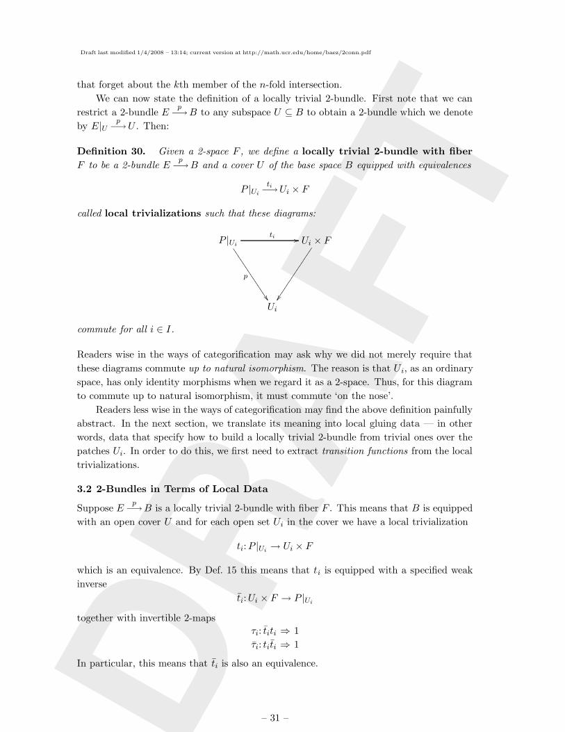
Definition 30. Given a 2-space F , we define a locally trivial 2-bundle with fiber
F to be a 2-bundle Ep−→B and a cover U of the base space B equipped with equivalences
P |Uiti−→Ui × F
called local trivializations such that these diagrams:
P |Ui
p
44444444444444ti // Ui × F
Ui
commute for all i ∈ I.
Readers wise in the ways of categorification may ask why we did not merely require that
these diagrams commute up to natural isomorphism. The reason is that Ui, as an ordinary
space, has only identity morphisms when we regard it as a 2-space. Thus, for this diagram
to commute up to natural isomorphism, it must commute ‘on the nose’.
Readers less wise in the ways of categorification may find the above definition painfully
abstract. In the next section, we translate its meaning into local gluing data — in other
words, data that specify how to build a locally trivial 2-bundle from trivial ones over the
patches Ui. In order to do this, we first need to extract transition functions from the local
trivializations.
3.2 2-Bundles in Terms of Local Data
Suppose Ep−→B is a locally trivial 2-bundle with fiber F . This means that B is equipped
with an open cover U and for each open set Ui in the cover we have a local trivialization
ti:P |Ui → Ui × F
which is an equivalence. By Def. 15 this means that ti is equipped with a specified weak
inverse
ti:Ui × F → P |Uitogether with invertible 2-maps
τi: titi ⇒ 1
τi: titi ⇒ 1
In particular, this means that ti is also an equivalence.
– 31 –
Draft last modified 1/4/2008 – 13:14; current version at http://math.ucr.edu/home/baez/2conn.pdf
DR
AFT
Now consider a double intersection Uij = Ui ∩ Uj. The composite of equivalences is
again an equivalence, so we get an autoequivalence
tj ti:Uij × F → Uij × F
that is, an equivalence from this 2-space to itself. By the commutative diagram in Def. 30,
this autoequivalence must act trivially on the Uij factor, so
tj ti(x, f) = (x, fgij(x))
for some smooth function gij from Uij to the smooth space of autoequivalences of the fiber
F . Note that we write these autoequivalences as acting on F from the right, as customary
in the theory of bundles. We call the functions gij transition functions, since they are
just categorified versions of the usual transition functions for locally trivial bundles.
In fact, for any smooth 2-space F there is a smooth 2-space AUT (F ) whose objects
are autoequivalences of F and whose morphisms are invertible 2-maps between these. The
transition functions are maps
gij :Uij → Ob(AUT (F )).
The 2-space AUT (F ) is a kind of 2-group, with composition of autoequivalences giving the
product. However, is not the sort of 2-group we have been considering here, because it does
not have ‘strict inverses’: the group laws involving inverses do not hold as equations, but
only up to specified isomorphisms that satisfy coherence laws of their own. So, AUT (F )
is a ‘coherent’ smooth 2-group in the sense of Baez and Lauda [3].
Next, consider a triple intersection Uijk = Ui ∩ Uj ∩ Uk. In an ordinary locally trivial
bundle the transition functions satisfy the equation gijgjk = gik, but in a locally trivial
2-bundle this holds only up to isomorphism. In other words, there is a smooth map
hijk:Uijk → Mor(AUT (F ))
such that for any x ∈ Uijk,
hijk(x): gij(x)gjk(x)∼−→ gik(x).
To see this, note that there is an invertible 2-map
tkτj ti : tk tjtj ti ⇒ tk ti
defined by horizontally composing τj with tk on the left and ti on the right. Since
tk tjtj ti(x, f) = (x, fgij(x)gjk(x))
while
tk ti(x, f) = (x, fgik(x))
we have
tkτj ti(x, f): (x, fgij(x)gjk(x))→ (x, fgik(x)).
– 32 –
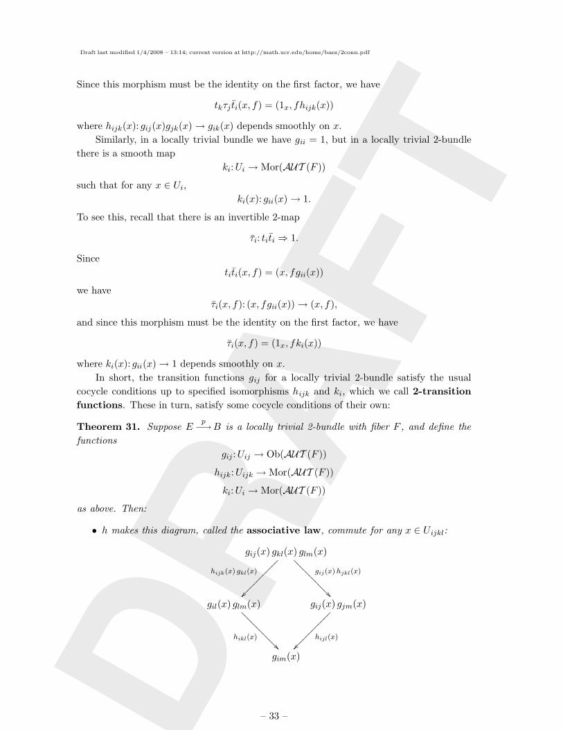
Draft last modified 1/4/2008 – 13:14; current version at http://math.ucr.edu/home/baez/2conn.pdf
DR
AFT
Since this morphism must be the identity on the first factor, we have
tkτj ti(x, f) = (1x, fhijk(x))
where hijk(x): gij(x)gjk(x)→ gik(x) depends smoothly on x.
Similarly, in a locally trivial bundle we have gii = 1, but in a locally trivial 2-bundle
there is a smooth map
ki:Ui → Mor(AUT (F ))
such that for any x ∈ Ui,ki(x): gii(x)→ 1.
To see this, recall that there is an invertible 2-map
τi: titi ⇒ 1.
Since
titi(x, f) = (x, fgii(x))
we have
τi(x, f): (x, fgii(x))→ (x, f),
and since this morphism must be the identity on the first factor, we have
τi(x, f) = (1x, fki(x))
where ki(x): gii(x)→ 1 depends smoothly on x.
In short, the transition functions gij for a locally trivial 2-bundle satisfy the usual
cocycle conditions up to specified isomorphisms hijk and ki, which we call 2-transition
functions. These in turn, satisfy some cocycle conditions of their own:
Theorem 31. Suppose Ep−→B is a locally trivial 2-bundle with fiber F , and define the
functions
gij :Uij → Ob(AUT (F ))
hijk:Uijk → Mor(AUT (F ))
ki:Ui → Mor(AUT (F ))
as above. Then:
• h makes this diagram, called the associative law, commute for any x ∈ Uijkl:
gij(x) gkl(x) glm(x)
gil(x) glm(x) gij(x) gjm(x)
gim(x)
gij(x)hjkl(x)
????????????
hijk(x) gkl(x)
hijl(x)
hikl(x)
????????????
– 33 –
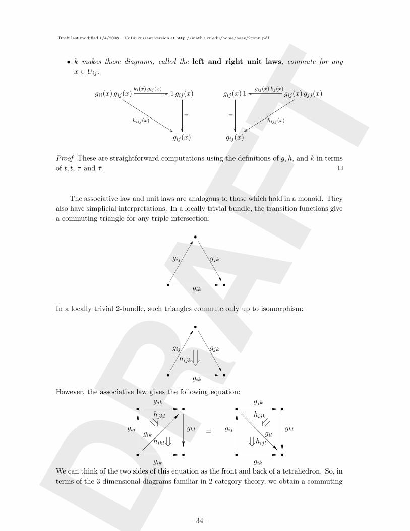
Draft last modified 1/4/2008 – 13:14; current version at http://math.ucr.edu/home/baez/2conn.pdf
DR
AFT
• k makes these diagrams, called the left and right unit laws, commute for any
x ∈ Uij:
gii(x) gij(x) 1 gij(x)
gij(x)
ki(x) gij(x)//
=
hiij(x)
%%KKKKKKKKKKKKKKKKKKgij(x) 1 gij(x) gjj(x)
gij(x)
gij(x) kj(x)oo
=
hijj(x)
yyssssssssssssssssss
Proof. These are straightforward computations using the definitions of g, h, and k in terms
of t, t, τ and τ . 2
The associative law and unit laws are analogous to those which hold in a monoid. They
also have simplicial interpretations. In a locally trivial bundle, the transition functions give
a commuting triangle for any triple intersection:
gij gjk
gik
In a locally trivial 2-bundle, such triangles commute only up to isomorphism:
gij gjk
gik
hijk
However, the associative law gives the following equation:
gikgik
hijkhjkl
gjkgjk
gklgijgklgij
hijlhikl
= gilgik
We can think of the two sides of this equation as the front and back of a tetrahedron. So, in
terms of the 3-dimensional diagrams familiar in 2-category theory, we obtain a commuting
– 34 –
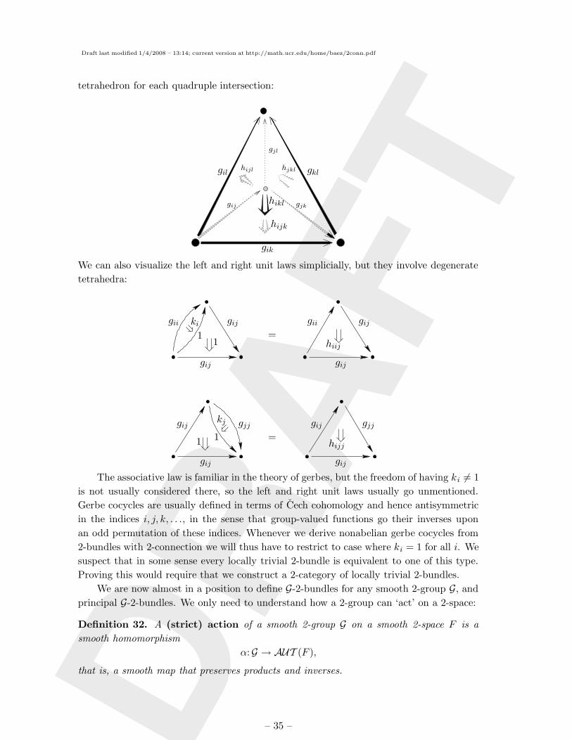
Draft last modified 1/4/2008 – 13:14; current version at http://math.ucr.edu/home/baez/2conn.pdf
DR
AFT
tetrahedron for each quadruple intersection:
gij gjk
gik
gil gkl
gjl
hijk
hikl
hjklhijl
We can also visualize the left and right unit laws simplicially, but they involve degenerate
tetrahedra:
gijgij
gijgij
gijgij
gijgij
giigii ki1
1=
hiij
=
gjjgjjkj
11 hijj
The associative law is familiar in the theory of gerbes, but the freedom of having ki 6= 1
is not usually considered there, so the left and right unit laws usually go unmentioned.
Gerbe cocycles are usually defined in terms of Cech cohomology and hence antisymmetric
in the indices i, j, k, . . ., in the sense that group-valued functions go their inverses upon
an odd permutation of these indices. Whenever we derive nonabelian gerbe cocycles from
2-bundles with 2-connection we will thus have to restrict to case where ki = 1 for all i. We
suspect that in some sense every locally trivial 2-bundle is equivalent to one of this type.
Proving this would require that we construct a 2-category of locally trivial 2-bundles.
We are now almost in a position to define G-2-bundles for any smooth 2-group G, and
principal G-2-bundles. We only need to understand how a 2-group can ‘act’ on a 2-space:
Definition 32. A (strict) action of a smooth 2-group G on a smooth 2-space F is a
smooth homomorphism
α:G → AUT (F ),
that is, a smooth map that preserves products and inverses.
– 35 –
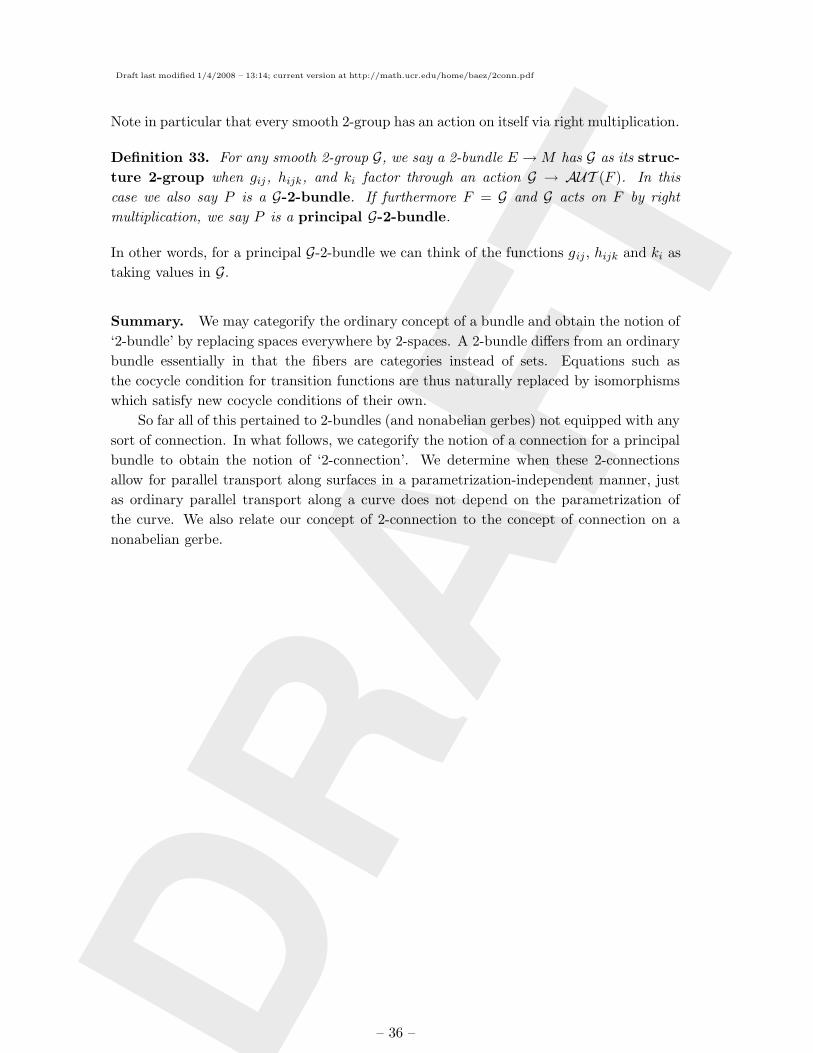
Draft last modified 1/4/2008 – 13:14; current version at http://math.ucr.edu/home/baez/2conn.pdf
DR
AFT
Note in particular that every smooth 2-group has an action on itself via right multiplication.
Definition 33. For any smooth 2-group G, we say a 2-bundle E →M has G as its struc-
ture 2-group when gij, hijk, and ki factor through an action G → AUT (F ). In this
case we also say P is a G-2-bundle. If furthermore F = G and G acts on F by right
multiplication, we say P is a principal G-2-bundle.
In other words, for a principal G-2-bundle we can think of the functions gij , hijk and ki as
taking values in G.
Summary. We may categorify the ordinary concept of a bundle and obtain the notion of
‘2-bundle’ by replacing spaces everywhere by 2-spaces. A 2-bundle differs from an ordinary
bundle essentially in that the fibers are categories instead of sets. Equations such as
the cocycle condition for transition functions are thus naturally replaced by isomorphisms
which satisfy new cocycle conditions of their own.
So far all of this pertained to 2-bundles (and nonabelian gerbes) not equipped with any
sort of connection. In what follows, we categorify the notion of a connection for a principal
bundle to obtain the notion of ‘2-connection’. We determine when these 2-connections
allow for parallel transport along surfaces in a parametrization-independent manner, just
as ordinary parallel transport along a curve does not depend on the parametrization of
the curve. We also relate our concept of 2-connection to the concept of connection on a
nonabelian gerbe.
– 36 –
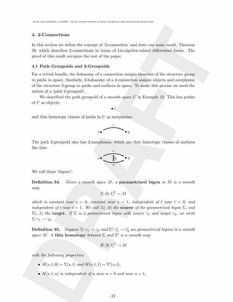
Draft last modified 1/4/2008 – 13:14; current version at http://math.ucr.edu/home/baez/2conn.pdf
DR
AFT
4. 2-Connections
In this section we define the concept of ‘2-connection’ and state our main result, Theorem
39, which describes 2-connections in terms of Lie-algebra-valued differential forms. The
proof of this result occupies the rest of the paper.
4.1 Path Groupoids and 2-Groupoids
For a trivial bundle, the holonomy of a connection assigns elements of the structure group
to paths in space. Similarly, 2-holonomy of a 2-connection assigns objects and morphisms
of the structure 2-group to paths and surfaces in space. To make this precise we need the
notion of a ‘path 2-groupoid’.
We described the path groupoid of a smooth space U in Example 12. This has points
of U as objects:
• x
and thin homotopy classes of paths in U as morphisms:
x •γ
'' • y
The path 2-groupoid also has 2-morphisms, which are thin homotopy classes of surfaces
like this:
x •γ1
''
γ2
77 • yΣ
We call these ‘bigons’:
Definition 34. Given a smooth space M , a parametrized bigon in M is a smooth
map
Σ: [0, 1]2 →M
which is constant near s = 0, constant near s = 1, independent of t near t = 0, and
independent of t near t = 1. We call Σ(·, 0) the source of the parametrized bigon Σ, and
Σ(·, 1) the target. If Σ is a parametrized bigon with source γ1 and target γ2, we write
Σ: γ1 → γ2.
Definition 35. Suppose Σ: γ1 → γ2 and Σ′: γ′1 → γ′2 are parametrized bigons in a smooth
space M . A thin homotopy between Σ and Σ′ is a smooth map
H: [0, 1]3 →M
with the following properties:
• H(s, t, 0) = Σ(s, t) and H(s, t, 1) = Σ′(s, t),
• H(s, t, u) is independent of u near u = 0 and near u = 1,
– 37 –
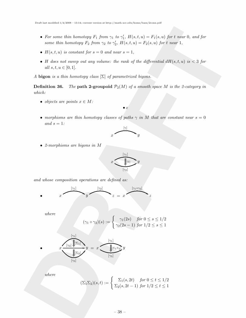
Draft last modified 1/4/2008 – 13:14; current version at http://math.ucr.edu/home/baez/2conn.pdf
DR
AFT
• For some thin homotopy F1 from γ1 to γ′1, H(s, t, u) = F1(s, u) for t near 0, and for
some thin homotopy F2 from γ2 to γ′2, H(s, t, u) = F2(s, u) for t near 1,
• H(s, t, u) is constant for s = 0 and near s = 1,
• H does not sweep out any volume: the rank of the differential dH(s, t, u) is < 3 for
all s, t, u ∈ [0, 1].
A bigon is a thin homotopy class [Σ] of parametrized bigons.
Definition 36. The path 2-groupoid P2(M) of a smooth space M is the 2-category in
which:
• objects are points x ∈M :
• x
• morphisms are thin homotopy classes of paths γ in M that are constant near s = 0
and s = 1:
x
[γ]
%% y
• 2-morphisms are bigons in M
x
[γ1]
%%
[γ2]
99[Σ]
y
and whose composition operations are defined as:
• x
[γ1]
%% y
[γ2]
%%z = x
[γ1γ2]
&&z
where
(γ1 γ2)(s) :=
γ1(2s) for 0 ≤ s ≤ 1/2
γ2(2s− 1) for 1/2 ≤ s ≤ 1
• x
[γ1]
[γ2] //[Σ1]
[γ3]
BB[Σ2]
y = x
[γ1]
%%
[γ3]
99[Σ1Σ2]
y
where
(Σ1Σ2)(s, t) :=
Σ1(s, 2t) for 0 ≤ t ≤ 1/2
Σ2(s, 2t− 1) for 1/2 ≤ t ≤ 1
– 38 –
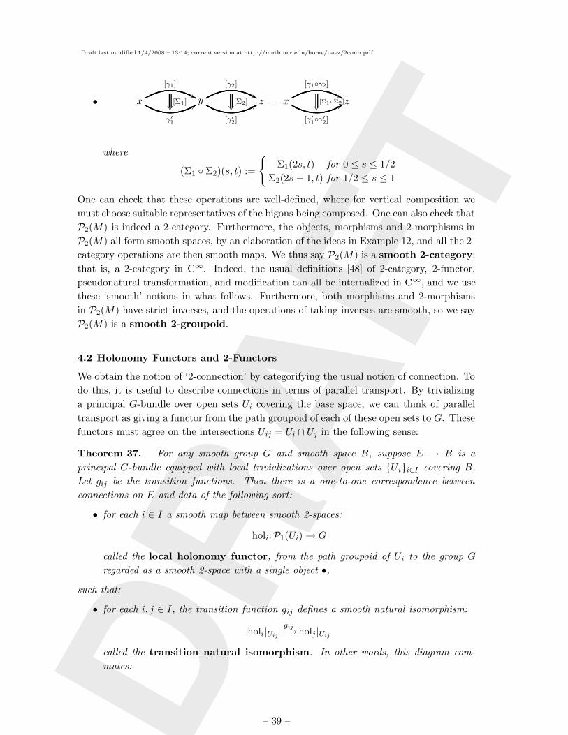
Draft last modified 1/4/2008 – 13:14; current version at http://math.ucr.edu/home/baez/2conn.pdf
DR
AFT
• x
[γ1]
%%
γ′1
99[Σ1]
y
[γ2]
%%
[γ′2]
99[Σ2]
z = x
[γ1γ2]
&&
[γ′1γ′2]
88[Σ1Σ2]
z
where
(Σ1 Σ2)(s, t) :=
Σ1(2s, t) for 0 ≤ s ≤ 1/2
Σ2(2s− 1, t) for 1/2 ≤ s ≤ 1
One can check that these operations are well-defined, where for vertical composition we
must choose suitable representatives of the bigons being composed. One can also check that
P2(M) is indeed a 2-category. Furthermore, the objects, morphisms and 2-morphisms in
P2(M) all form smooth spaces, by an elaboration of the ideas in Example 12, and all the 2-
category operations are then smooth maps. We thus say P2(M) is a smooth 2-category:
that is, a 2-category in C∞. Indeed, the usual definitions [48] of 2-category, 2-functor,
pseudonatural transformation, and modification can all be internalized in C∞, and we use
these ‘smooth’ notions in what follows. Furthermore, both morphisms and 2-morphisms
in P2(M) have strict inverses, and the operations of taking inverses are smooth, so we say
P2(M) is a smooth 2-groupoid.
4.2 Holonomy Functors and 2-Functors
We obtain the notion of ‘2-connection’ by categorifying the usual notion of connection. To
do this, it is useful to describe connections in terms of parallel transport. By trivializing
a principal G-bundle over open sets Ui covering the base space, we can think of parallel
transport as giving a functor from the path groupoid of each of these open sets to G. These
functors must agree on the intersections Uij = Ui ∩ Uj in the following sense:
Theorem 37. For any smooth group G and smooth space B, suppose E → B is a
principal G-bundle equipped with local trivializations over open sets Uii∈I covering B.
Let gij be the transition functions. Then there is a one-to-one correspondence between
connections on E and data of the following sort:
• for each i ∈ I a smooth map between smooth 2-spaces:
holi:P1(Ui)→ G
called the local holonomy functor, from the path groupoid of Ui to the group G
regarded as a smooth 2-space with a single object •,such that:
• for each i, j ∈ I, the transition function gij defines a smooth natural isomorphism:
holi|Uijgij−→holj |Uij
called the transition natural isomorphism. In other words, this diagram com-
mutes:
– 39 –
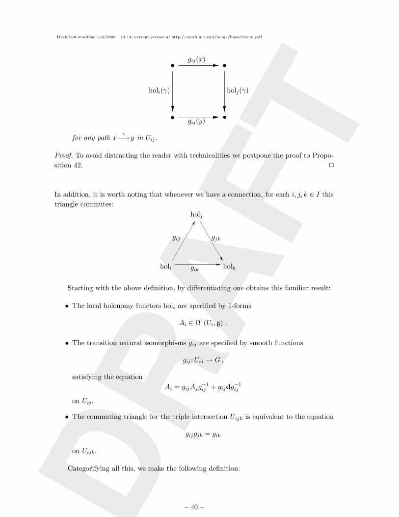
Draft last modified 1/4/2008 – 13:14; current version at http://math.ucr.edu/home/baez/2conn.pdf
DR
AFT
gij(x)
gij(y)
holi(γ) holj(γ)
for any path xγ−→ y in Uij.
Proof. To avoid distracting the reader with technicalities we postpone the proof to Propo-
sition 42. 2
In addition, it is worth noting that whenever we have a connection, for each i, j, k ∈ I this
triangle commutes:
gij gjk
gikholi
holj
holk
Starting with the above definition, by differentiating one obtains this familiar result:
• The local holonomy functors holi are specified by 1-forms
Ai ∈ Ω1(Ui, g) .
• The transition natural isomorphisms gij are specified by smooth functions
gij :Uij → G ,
satisfying the equation
Ai = gijAjg−1ij + gijdg
−1ij
on Uij .
• The commuting triangle for the triple intersection Uijk is equivalent to the equation
gijgjk = gik
on Uijk.
Categorifying all this, we make the following definition:
– 40 –
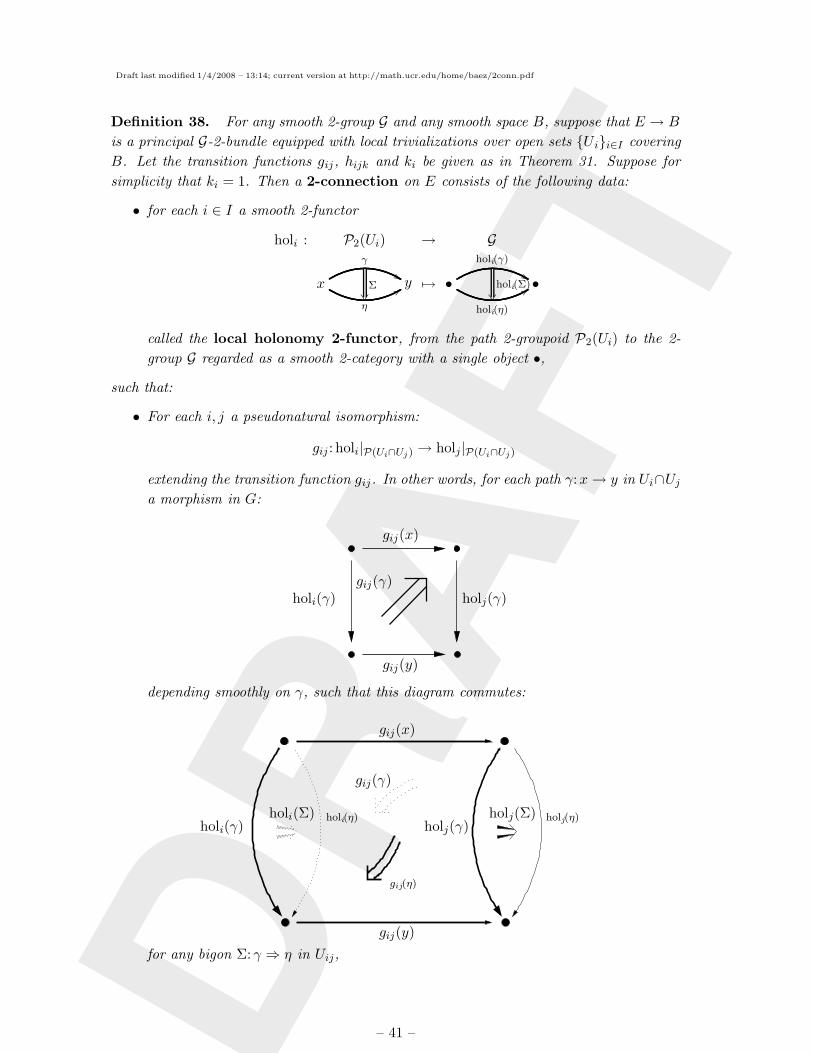
Draft last modified 1/4/2008 – 13:14; current version at http://math.ucr.edu/home/baez/2conn.pdf
DR
AFT
Definition 38. For any smooth 2-group G and any smooth space B, suppose that E → B
is a principal G-2-bundle equipped with local trivializations over open sets Uii∈I covering
B. Let the transition functions gij, hijk and ki be given as in Theorem 31. Suppose for
simplicity that ki = 1. Then a 2-connection on E consists of the following data:
• for each i ∈ I a smooth 2-functor
holi : P2(Ui) → G
x
γ
%%
η
99Σ
y 7→ •holi(γ)
%%
holi(η)
99holi(Σ)
•
called the local holonomy 2-functor, from the path 2-groupoid P2(Ui) to the 2-
group G regarded as a smooth 2-category with a single object •,
such that:
• For each i, j a pseudonatural isomorphism:
gij : holi|P(Ui∩Uj) → holj|P(Ui∩Uj)
extending the transition function gij. In other words, for each path γ:x→ y in Ui∩Uja morphism in G:
gij(x)
gij(y)
holi(γ) holj(γ)gij(γ)
depending smoothly on γ, such that this diagram commutes:
holi(γ)holi(η)holi(Σ)
gij(η)
gij(γ)
gij(x)
gij(y)
holj(γ)holj(η)holj(Σ)
for any bigon Σ: γ ⇒ η in Uij,
– 41 –
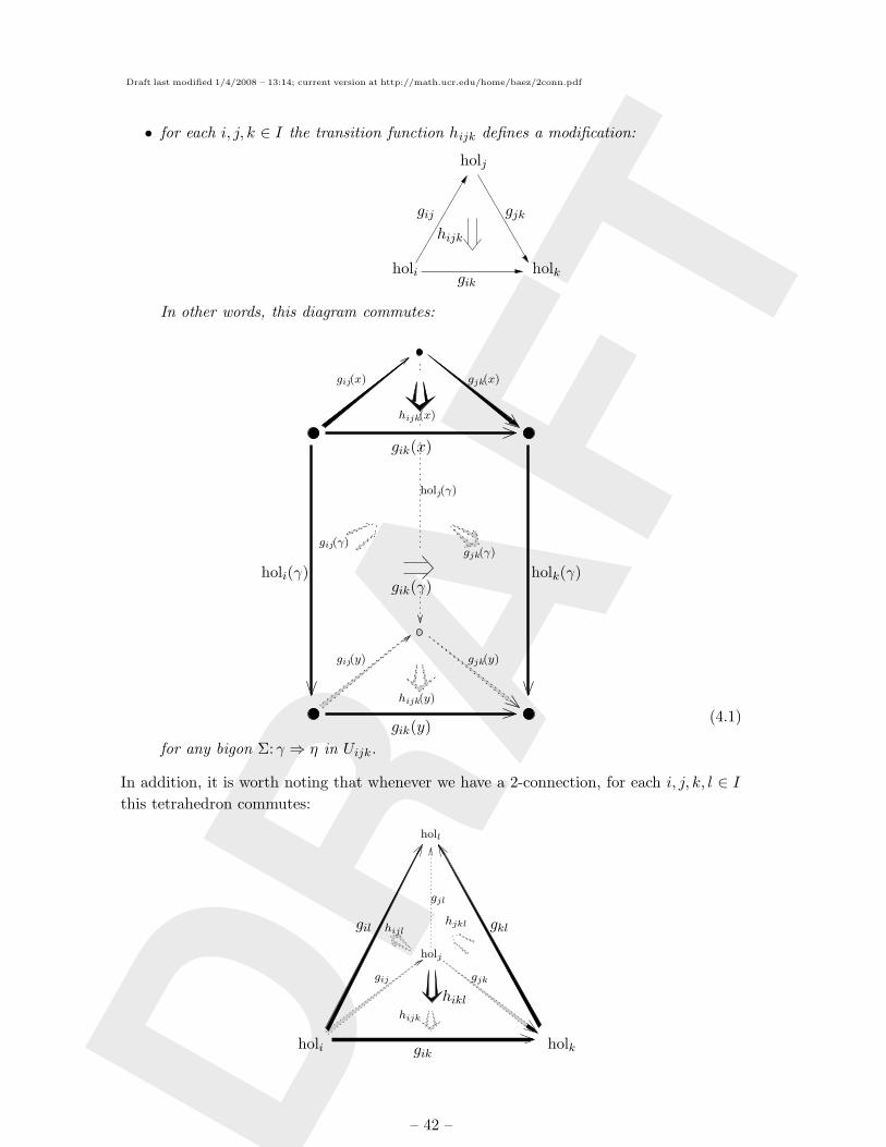
Draft last modified 1/4/2008 – 13:14; current version at http://math.ucr.edu/home/baez/2conn.pdf
DR
AFT
• for each i, j, k ∈ I the transition function hijk defines a modification:
holi
holj
holk
gij gjk
gik
hijk
In other words, this diagram commutes:
holk(γ)holi(γ)
holj(γ)
gik(y)
gik(x)
gij(y)
gij(x)
gjk(y)
gjk(x)
hijk(y)
hijk(x)
gik(γ)
gij(γ)gjk(γ)
(4.1)
for any bigon Σ: γ ⇒ η in Uijk.
In addition, it is worth noting that whenever we have a 2-connection, for each i, j, k, l ∈ Ithis tetrahedron commutes:
gij gjk
gik
gil gkl
gjl
holi holk
holj
holl
hijk
hikl
hjklhijl
– 42 –
Draft last modified 1/4/2008 – 13:14; current version at http://math.ucr.edu/home/baez/2conn.pdf
DR
AFT
In analogy to the situation for ordinary connections on bundles, one would like to
obtain 2-connections from Lie-algebra-valued differential forms. This is our next result. In
what follows, (G,H, t, α) will be the smooth crossed module corresponding to the smooth
2-group G. We think of the transition function gij as taking values in Ob(G) = G, and
think of hijk as taking values in H. Actually hijk takes values in Mor(G) ∼= GoH, but its
G component is determined by its source, so only its H component is interesting. In these
terms, the fact that
hijk(x): gij(x)gjk(x)∼−→ gik(x)
translates into the equation
gij(x) gjk(x) t(hijk(x)) = gik(x),
and the associative law of Theorem 31 (i.e. the above tetrahedron) becomes a cocycle
condition familiar from the theory of nonabelian gerbes:
hijk hikl = α(gij)(hjkl)hijl . (4.2)
Theorem 39. For any smooth 2-group G, suppose that E → B is a principal G-2-bundle
equipped with local trivializations over open sets Uii∈I covering B, with the transition
functions gij, hijk and ki given as in Theorem 31. Suppose for simplicity that ki = 1.
Let (G,H, t, α) be the smooth crossed module corresponding to G, and let (g, h, dt, dα) be
the corresponding differential crossed module. Then there is a one-to-one correspondence
between 2-connections on E and Lie-algebra-valued differential forms (Ai, Bi, aij) satisfying
certain equations, as follows:
1. The local holonomy 2-functor holi is specified by differential forms
Ai ∈ Ω1(Ui, g)
Bi ∈ Ω2(Ui, h)
satisfying
FAi + dt(Bi) = 0 ,
where FAi = dAi +Ai ∧Ai is the curvature 2-form of Ai.
2. The transition pseudonatural isomorphism holigij−→holj is specified by the transition
functions gij together with differential forms
aij ∈ Ω1(Uij , h)
satisfying the equations:
Ai = gijAjg−1ij + gijdg
−1ij
Bi = α(gij)(Bi) + kij
on Uij, where
kij = daij + aij ∧ aij + dα(Ai) ∧ aij .
– 43 –
Draft last modified 1/4/2008 – 13:14; current version at http://math.ucr.edu/home/baez/2conn.pdf
DR
AFT
3. The modification gij gjkhijk−→ gik is specified by the transition functions hijk. For this,
the differential forms aij are required to satisfy the equation:
aij + α(gij)ajk = hijk aik h−1ijk + dhijk h
−1ijk + dα(Ai)(hijk)h−1
ijk.
on Uijk.
Proof. The idea behind the Proof of part 1. is sketched in §5.1. The full proof is the content
of §6.5. The proof for part 2. is given in §5.2. Again, the idea is quite simple, but the proof
needs some facts only developed in §6. The proof of part 3. appears in §5.3. Part 4. was
discussed before in §3.2. 2
– 44 –
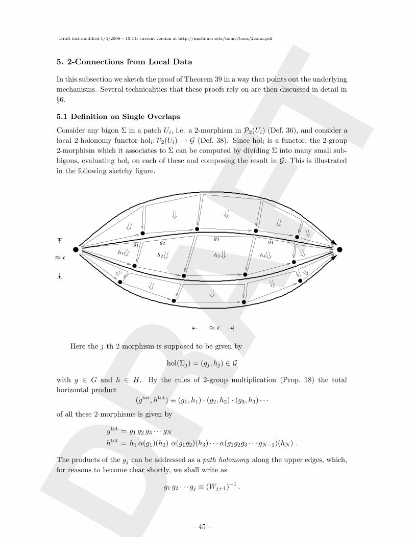
Draft last modified 1/4/2008 – 13:14; current version at http://math.ucr.edu/home/baez/2conn.pdf
DR
AFT
5. 2-Connections from Local Data
In this subsection we sketch the proof of Theorem 39 in a way that points out the underlying
mechanisms. Several technicalities that these proofs rely on are then discussed in detail in
§6.
5.1 Definition on Single Overlaps
Consider any bigon Σ in a patch Ui, i.e. a 2-morphism in P2(Ui) (Def. 36), and consider a
local 2-holonomy functor holi:P2(Ui) → G (Def. 38). Since holi is a functor, the 2-group
2-morphism which it associates to Σ can be computed by dividing Σ into many small sub-
bigons, evaluating holi on each of these and composing the result in G. This is illustrated
in the following sketchy figure.
g1
h1
g2
h2
g3
h3
g4
h4≈ ε
≈ ε
Here the j-th 2-morphism is supposed to be given by
hol(Σj) = (gj , hj) ∈ G
with g ∈ G and h ∈ H. By the rules of 2-group multiplication (Prop. 18) the total
horizontal product
(gtot, htot) ≡ (g1, h1) · (g2, h2) · (g3, h3) · · ·of all these 2-morphisms is given by
gtot = g1 g2 g3 · · · gNhtot = h1 α(g1)(h2) α(g1g2)(h3) · · ·α(g1g2g3 · · · gN−1)(hN ) .
The products of the gj can be addressed as a path holonomy along the upper edges, which,
for reasons to become clear shortly, we shall write as
g1 g2 · · · gj ≡ (Wj+1)−1 .
– 45 –
Draft last modified 1/4/2008 – 13:14; current version at http://math.ucr.edu/home/baez/2conn.pdf
DR
AFT
Now suppose the group elements come from algebra elements Aj ∈ g and Bj ∈ h as
gj ≡ exp(εAj)
hj ≡ exp(ε2Bj
)(5.1)
where
ε ≡ 1/N ,
then
htot = 1 + ε2N∑
j=1
α(W−1j
)(Bj) +O
(ε4).
Using the notation
Wj ≡ W (1− jε, 1)
Bj ≡ B(1− εj)
we have
htot = 1 + ε
1∫
0
dσ α(W−1(σ, 1)
)(B(σ)) +O
(ε3).
Finally, imagine that the G-labels htotk of many such thin horizontal rows of ‘surface ele-
ments’ are composed vertically. Each of them comes from algebra elements
Bk(σ) ≡ B(σ, kε)
and holonomies
Wk(σ, 1) ≡Wkε(σ, 1)
as
htotk ≡ 1 + ε
1∫
0
dσ α(W−1kε (σ, 1)
)(B(σ, kε)) +O
(ε3).
In the limit of vanishing ε their total vertical product is
limε=1/N→0
htot0 htot
ε htot2ε · · · htot
1 = P exp
1∫
0
dτ A(τ)
for
A(τ) =
1∫
0
dσ α(W−1τ (σ, 1)
)(B(σ, τ)) , (5.2)
P where denotes path ordering with respect to τ .
Thinking of each of these vertical rows of surface elements as paths (in the limit
ε→ 0), this shows roughly how the computation of total 2-group elements from vertical and
– 46 –
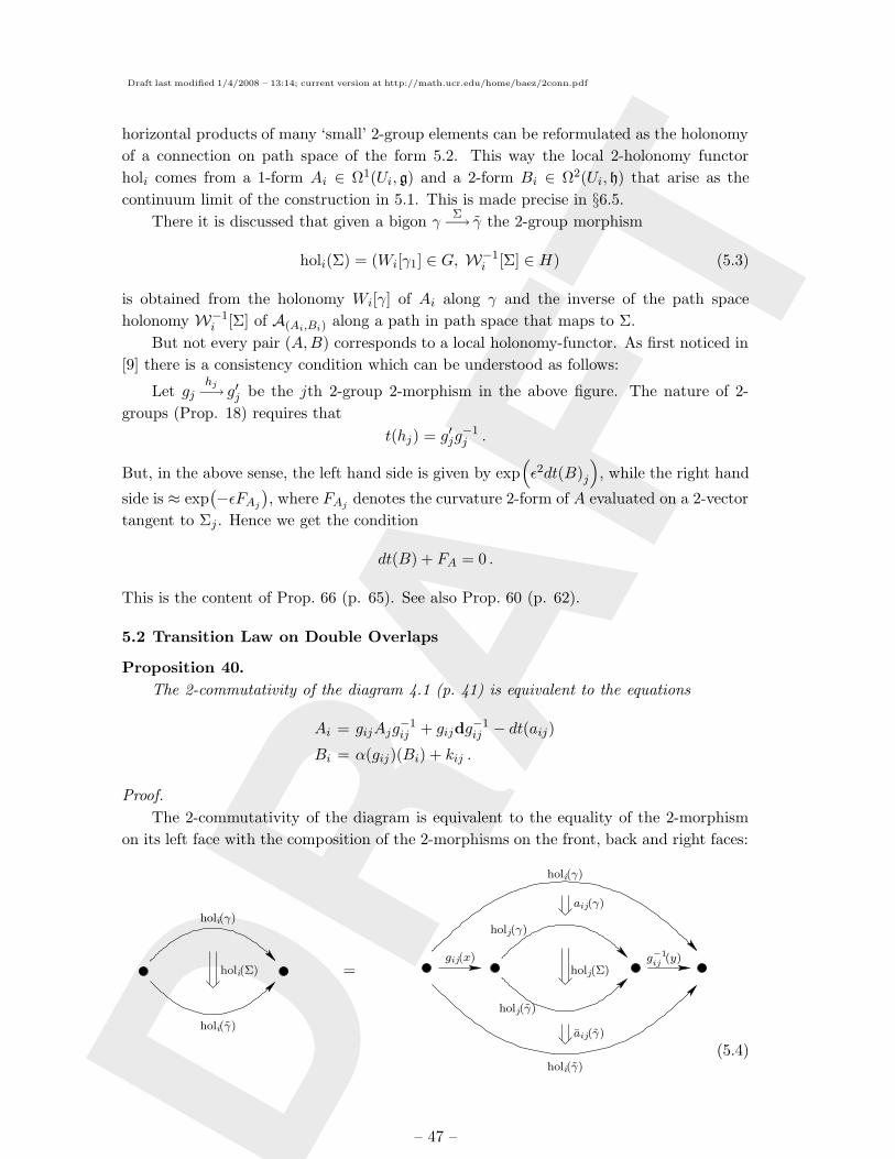
Draft last modified 1/4/2008 – 13:14; current version at http://math.ucr.edu/home/baez/2conn.pdf
DR
AFT
horizontal products of many ‘small’ 2-group elements can be reformulated as the holonomy
of a connection on path space of the form 5.2. This way the local 2-holonomy functor
holi comes from a 1-form Ai ∈ Ω1(Ui, g) and a 2-form Bi ∈ Ω2(Ui, h) that arise as the
continuum limit of the construction in 5.1. This is made precise in §6.5.
There it is discussed that given a bigon γΣ−→ γ the 2-group morphism
holi(Σ) = (Wi[γ1] ∈ G, W−1i [Σ] ∈ H) (5.3)
is obtained from the holonomy Wi[γ] of Ai along γ and the inverse of the path space
holonomy W−1i [Σ] of A(Ai,Bi) along a path in path space that maps to Σ.
But not every pair (A,B) corresponds to a local holonomy-functor. As first noticed in
[9] there is a consistency condition which can be understood as follows:
Let gjhj−→ g′j be the jth 2-group 2-morphism in the above figure. The nature of 2-
groups (Prop. 18) requires that
t(hj) = g′jg−1j .
But, in the above sense, the left hand side is given by exp(ε2dt(B)j
), while the right hand
side is ≈ exp(−εFAj
), where FAj denotes the curvature 2-form of A evaluated on a 2-vector
tangent to Σj . Hence we get the condition
dt(B) + FA = 0 .
This is the content of Prop. 66 (p. 65). See also Prop. 60 (p. 62).
5.2 Transition Law on Double Overlaps
Proposition 40.
The 2-commutativity of the diagram 4.1 (p. 41) is equivalent to the equations
Ai = gijAjg−1ij + gijdg
−1ij − dt(aij)
Bi = α(gij)(Bi) + kij .
Proof.
The 2-commutativity of the diagram is equivalent to the equality of the 2-morphism
on its left face with the composition of the 2-morphisms on the front, back and right faces:
holi(Σ) holj(Σ)
holi(γ)
holi(γ)
holj(γ)
holj(γ)
gij(x) g−1ij (y)
aij(γ)
aij(γ)
=
holi(γ)
holi(γ)
(5.4)
– 47 –
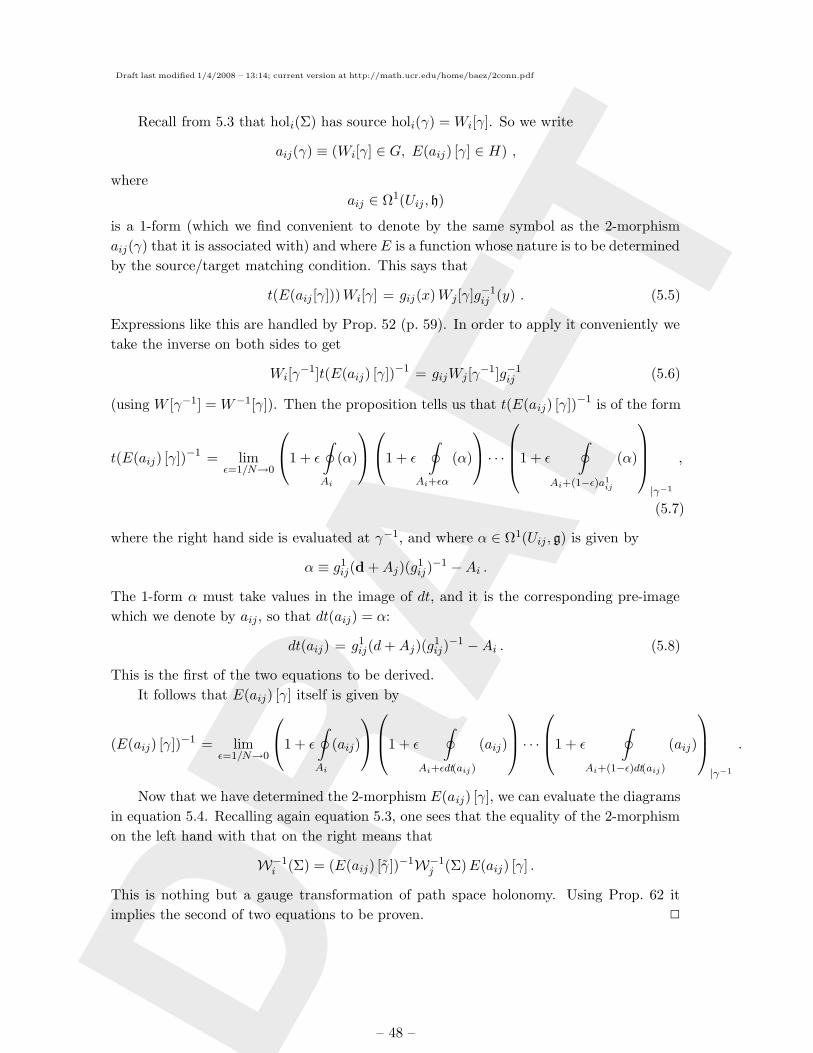
Draft last modified 1/4/2008 – 13:14; current version at http://math.ucr.edu/home/baez/2conn.pdf
DR
AFT
Recall from 5.3 that holi(Σ) has source holi(γ) = Wi[γ]. So we write
aij(γ) ≡ (Wi[γ] ∈ G, E(aij) [γ] ∈ H) ,
where
aij ∈ Ω1(Uij, h)
is a 1-form (which we find convenient to denote by the same symbol as the 2-morphism
aij(γ) that it is associated with) and where E is a function whose nature is to be determined
by the source/target matching condition. This says that
t(E(aij [γ]))Wi[γ] = gij(x)Wj[γ]g−1ij (y) . (5.5)
Expressions like this are handled by Prop. 52 (p. 59). In order to apply it conveniently we
take the inverse on both sides to get
Wi[γ−1]t(E(aij) [γ])−1 = gijWj[γ
−1]g−1ij (5.6)
(using W [γ−1] = W−1[γ]). Then the proposition tells us that t(E(aij) [γ])−1 is of the form
t(E(aij) [γ])−1 = limε=1/N→0
1 + ε
∮
Ai
(α)
1 + ε
∮
Ai+εα
(α)
· · ·
1 + ε
∮
Ai+(1−ε)a1ij
(α)
|γ−1
,
(5.7)
where the right hand side is evaluated at γ−1, and where α ∈ Ω1(Uij , g) is given by
α ≡ g1ij(d +Aj)(g
1ij)−1 −Ai .
The 1-form α must take values in the image of dt, and it is the corresponding pre-image
which we denote by aij, so that dt(aij) = α:
dt(aij) = g1ij(d+Aj)(g
1ij)−1 −Ai . (5.8)
This is the first of the two equations to be derived.
It follows that E(aij) [γ] itself is given by
(E(aij) [γ])−1 = limε=1/N→0
1 + ε
∮
Ai
(aij)
1 + ε
∮
Ai+εdt(aij )
(aij)
· · ·
1 + ε
∮
Ai+(1−ε)dt(aij)
(aij)
|γ−1
.
Now that we have determined the 2-morphism E(aij) [γ], we can evaluate the diagrams
in equation 5.4. Recalling again equation 5.3, one sees that the equality of the 2-morphism
on the left hand with that on the right means that
W−1i (Σ) = (E(aij) [γ])−1W−1
j (Σ)E(aij) [γ] .
This is nothing but a gauge transformation of path space holonomy. Using Prop. 62 it
implies the second of two equations to be proven. 2
– 48 –
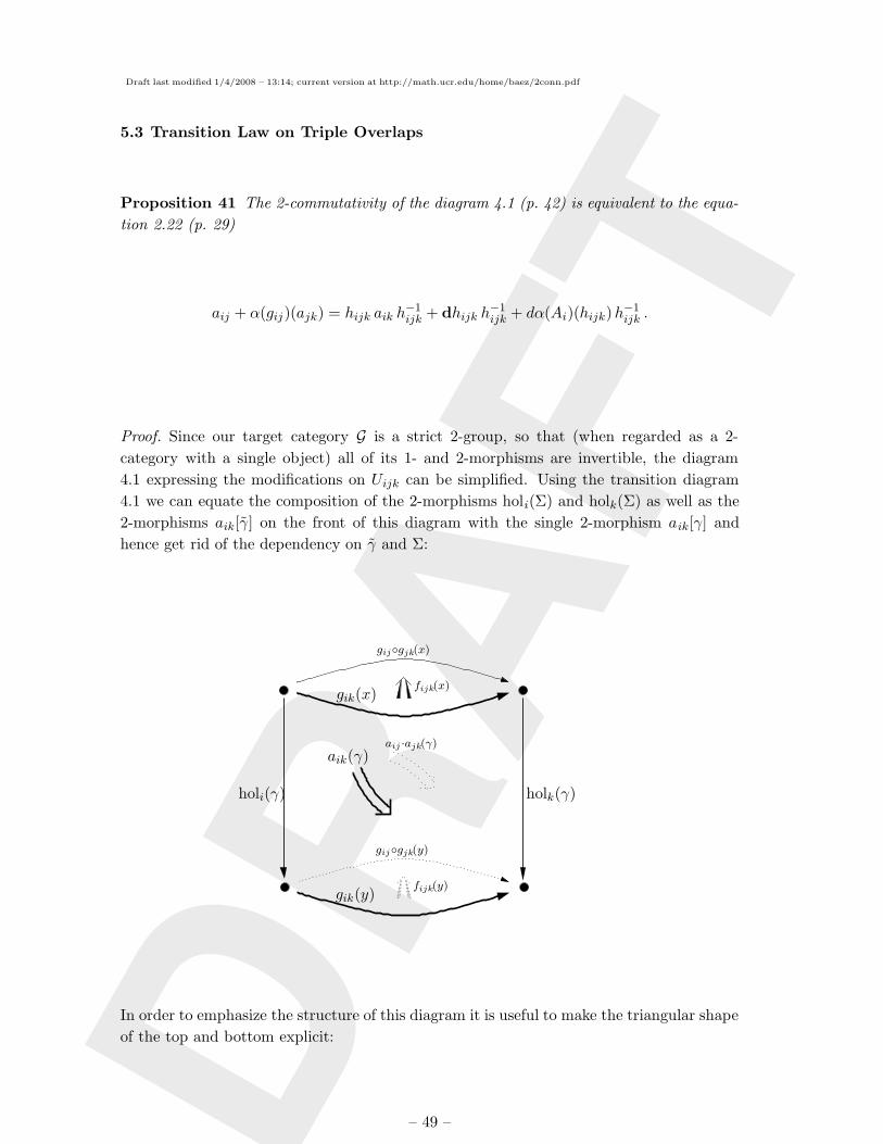
Draft last modified 1/4/2008 – 13:14; current version at http://math.ucr.edu/home/baez/2conn.pdf
DR
AFT
5.3 Transition Law on Triple Overlaps
Proposition 41 The 2-commutativity of the diagram 4.1 (p. 42) is equivalent to the equa-
tion 2.22 (p. 29)
aij + α(gij)(ajk) = hijk aik h−1ijk + dhijk h
−1ijk + dα(Ai)(hijk)h−1
ijk .
Proof. Since our target category G is a strict 2-group, so that (when regarded as a 2-
category with a single object) all of its 1- and 2-morphisms are invertible, the diagram
4.1 expressing the modifications on Uijk can be simplified. Using the transition diagram
4.1 we can equate the composition of the 2-morphisms holi(Σ) and holk(Σ) as well as the
2-morphisms aik[γ] on the front of this diagram with the single 2-morphism aik[γ] and
hence get rid of the dependency on γ and Σ:
holi(γ)
aik(γ)aij ·ajk(γ)
gik(x)
gijgjk(x)
fijk(x)
gik(y)
gijgjk(y)
fijk(y)
holk(γ)
In order to emphasize the structure of this diagram it is useful to make the triangular shape
of the top and bottom explicit:
– 49 –
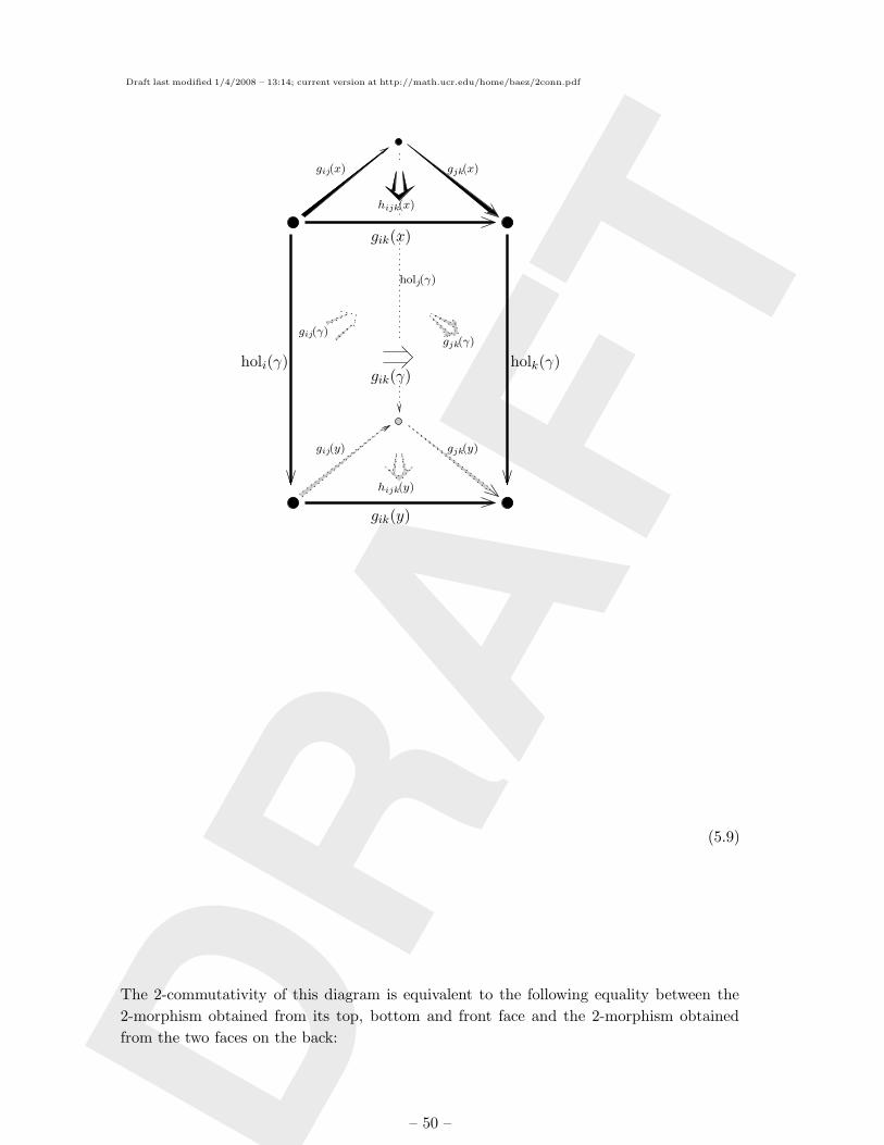
Draft last modified 1/4/2008 – 13:14; current version at http://math.ucr.edu/home/baez/2conn.pdf
DR
AFTholk(γ)holi(γ)
holj(γ)
gik(y)
gik(x)
gij(y)
gij(x)
gjk(y)
gjk(x)
hijk(y)
hijk(x)
gik(γ)
gij(γ)gjk(γ)
(5.9)
The 2-commutativity of this diagram is equivalent to the following equality between the
2-morphism obtained from its top, bottom and front face and the 2-morphism obtained
from the two faces on the back:
– 50 –
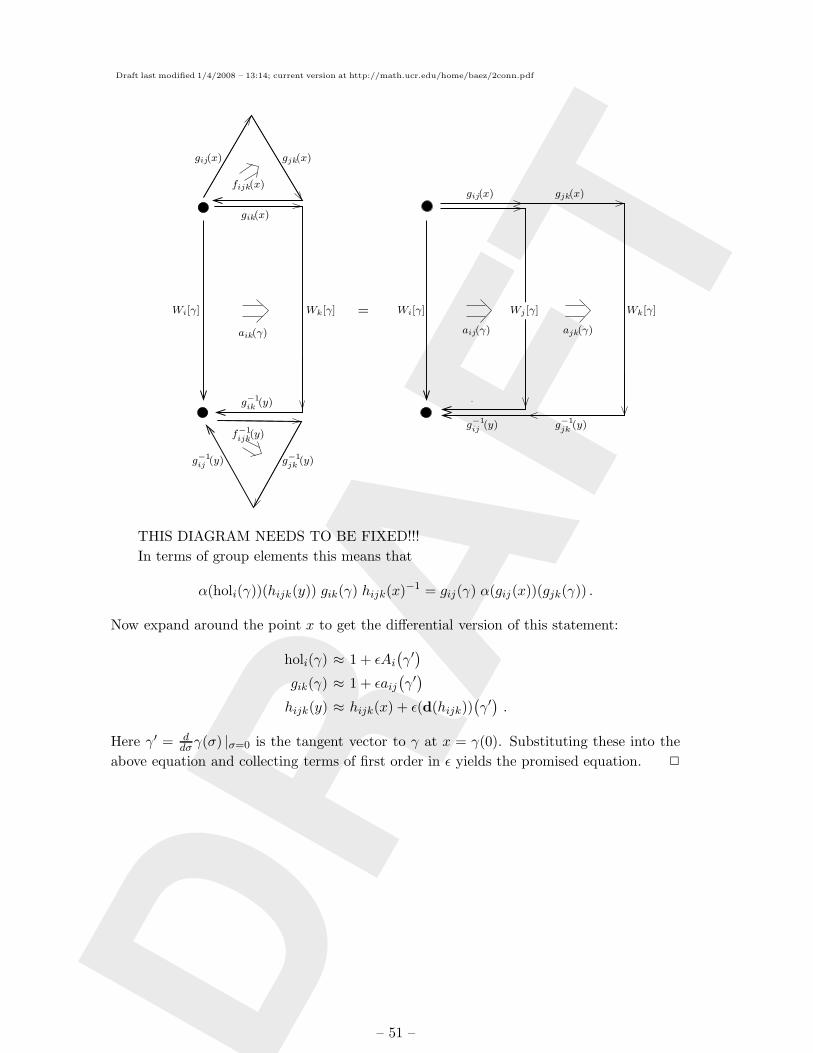
Draft last modified 1/4/2008 – 13:14; current version at http://math.ucr.edu/home/baez/2conn.pdf
DR
AFTaik(γ)
Wi[γ] Wk[γ]
fijk(x)
gij(x) gjk(x)
gik(x)
g−1ik (y)
g−1jk (y)g−1
ij (y)
f−1ijk(y)
=
gij(x) gjk(x)
g−1ij (y) g−1
jk (y)
Wi[γ] Wj [γ] Wk[γ]
aij(γ) ajk(γ)
THIS DIAGRAM NEEDS TO BE FIXED!!!
In terms of group elements this means that
α(holi(γ))(hijk(y)) gik(γ) hijk(x)−1 = gij(γ) α(gij(x))(gjk(γ)) .
Now expand around the point x to get the differential version of this statement:
holi(γ) ≈ 1 + εAi(γ′)
gik(γ) ≈ 1 + εaij(γ′)
hijk(y) ≈ hijk(x) + ε(d(hijk))(γ′).
Here γ′ = ddσγ(σ) |σ=0 is the tangent vector to γ at x = γ(0). Substituting these into the
above equation and collecting terms of first order in ε yields the promised equation. 2
– 51 –
Draft last modified 1/4/2008 – 13:14; current version at http://math.ucr.edu/home/baez/2conn.pdf
DR
AFT
6. 2-Connections in Terms of Connections on Path Space
6.1 Connections on Smooth Spaces
In this section we prove Proposition 37 and in the process develop some useful machinery
concerning path spaces. To prove this proposition, it suffices to show it in the special case
of a trivial bundle (EXPLAIN WHY):
Proposition 42. Let G be a smooth group and X a smooth space. Given any g-valued
1-form A on X, there is a smooth map between smooth 2-spaces
hol:P1(X)→ G
given by
hol([γ]) = P exp
∫
γA
where γ is any representative of the thin homotopy class [γ]. This gives a one-to-one
correspondence between elements A ∈ Ω1(X, g) and smooth maps hol:P1(X)→ G.
Proof. Any g-valued 1-form A on X defines a smooth map of 2-spaces hol:P1(X) → G
via the above formula, since we are assuming all our smooth groups are exponentiable
(see Example 21). We must show that any smooth functor hol:P1(X) → G comes from a
unique g-valued 1-form A in this way. We construct A by differentiating hol.
To do this, we must clarify the relation between morphisms in P1(X) and paths in X.
Recall that morphisms in P1(X) are equivalence classes of smooth maps γ: [0, 1] → X for
which γ(t) is constant for t near 0 and t near 1. Let PX stand for the space of all smooth
maps γ: [0, 1] → X.
Lemma 43. Suppose f : [0, 1] → [0, 1] is any smooth function with f(t) = 0 for t near 0
and f(t) = 1 for t near 1. Then there is a smooth map
p:PX → Mor(P1(X))
γ 7→ [γ f ]
where [γ f ] is the thin homotopy class of γ f . Moreover, p does not depend on the choice
of f .
Proof. The map p is clearly well-defined for any fixed f of the above sort; to show p is
smooth it suffices to show that the map
PX → PX
γ 7→ γ f
is smooth, which is straightforward. To show the map p is independent of f , suppose
f0, f1: [0, 1] → [0, 1] are both smooth functions that equal 0 near 0 and 1 near 1. Then
there exists a smooth function F : [0, 1]2 → [0, 1] such that:
– 52 –
Draft last modified 1/4/2008 – 13:14; current version at http://math.ucr.edu/home/baez/2conn.pdf
DR
AFT
• F (s, t) = f0(t) for s near 0
• F (s, t) = f1(t) for s near 1
• F (s, t) = 0 for t near 0
• F (s, t) = 1 for t near 1
It follows that
H(s, t) = γ(F (s, t))
is a thin homotopy from γ f0 to γ f1, so [γ f0] = [γ f1]. 2
We also need to consider Moore paths, which are smooth maps γ: [0, T ] → X for
arbitrary T ≥ 0. Note that a Moore path for T = 0 is just a point of X. We denote the set
of all Moore paths by MX. This becomes a smooth space where a plot (see the Appendix)
is a functionφ:Rn → MX
z 7→ φz
such that φz: [0, Tz ] → X, where Tz ∈ [0,∞] is a smooth function of z and φz(t) ∈ X is a
smooth function of z and t.
Here is the relation between Moore paths and paths parametrized by the unit interval:
Lemma 44 There is a smooth map
q:MX → PX
sending any Moore path γ: [0, T ]→ X to the path
(qγ)(t) = γ(T t).
Proof. Straightforward. 2
Using the smooth maps
MXq−→PX
p−→Mor(P1(X))
we can define holonomies for Moore paths. Namely, given any smooth map hol:P1(X)→ G,
we get a smooth map
Hol := hol q p
assigning an element of G to any Moore path.
To prove the lemma, it suffices to show there exists a unique A ∈ Ω1(X, g) with
Hol(γ) = P exp
∫
γA
– 53 –
Draft last modified 1/4/2008 – 13:14; current version at http://math.ucr.edu/home/baez/2conn.pdf
DR
AFT
for any Moore path γ: [0, T ] → X with T > 0. For this, it suffices to show there exists a
unique A such that for any Moore path γ: [0, T ]→ X with T > 0 we have
d
dsHol(γs) = A(γ′(s))Hol(γs) (6.1)
for all s ∈ [0, T ], where γs: [0, s]→ X is the Moore path given by restricting γ to [0, s].
In fact, it suffices to show there exists a unique A such that equation (6.1) holds
at s = 0. The reason is that for any s0 ∈ [0, T ] we can write the Moore path γ as a
‘concatenation’ of the Moore paths γs0 and η: [0, T − s0]→ X, where
η(t) = γ(t− s0).
So, since hol is a functor, we have
Hol(γs) = Hol(ηs−s0)Hol(γs0)
for s0 ≤ s ≤ T . It follows that
ddsHol(γs)|s=s0 = d
dsHol(ηs−s0)Hol(γs0)|s=s0
= ddsHol(ηs)|s=0 Hol(γs0).
So, if equation (6.1) holds at s = 0 for all Moore paths (in particular for η), we have
ddsHol(γs)|s=s0 = A(η′(0))Hol(η0)Hol(γs0)
= A(γ′(s0))Hol(γs0)
since Hol(η0) = 1 and η′(0) = γ′(s0). Thus, we have shown that equation (6.1) holds for γ
at s = s0, given that it holds for η at s = 0.
In short, we must show there exists a unique g-valued 1-form A such that for any
Moore path γ: [0, T ]→ X with T > 0,
d
dsHol(γs)|s=0 = A(γ′(0)).
Since any 1-form on X is determined by its values on tangent vectors of paths (see the
Appendix), this formula uniquely determines A. However, we need to check that A exists:
in other words, that it is well-defined and smooth. For the first, suppose we have two
Moore paths γ and η starting at x ∈ X with γ ′(0) = η′(0); we need to check that
d
dsHol(γs)|s=0 =
d
dsHol(ηs)|s=0.
For this, it suffices by the chain rule to check that
d
dsγs|s=0 =
d
dsηs|s=0
as tangent vectors in MX.
– 54 –
Draft last modified 1/4/2008 – 13:14; current version at http://math.ucr.edu/home/baez/2conn.pdf
DR
AFT
To check this, note that there is a smooth map
r:MX →MMX
sending any Moore path γ: [0, T ]→ X to the Moore path Γ: [0, T ]→MX given by Γ(s)(t) =
γs(t). Quite generally, the tangent vector of a Moore path in a smooth space can be thought
of as an equivalence class of Moore paths (see the Appendix). In particular, the tangent
vector γ′(0) ∈ TxX is an equivalence class of Moore paths in X starting at x. The smooth
map r sends any Moore path in this equivalence class to a Moore path in MX representing
the tangent vector ddsγs|s=0. Since γ′(0) = η′(0), γ and η lie in the same equivalence class,
so rγ and rη lie in the same equivalence class, which means that
d
dsγs|s=0 =
d
dsηs|s=0
as desired.
NEED TO CHECK SMOOTHNESS.... 2
6.2 More stuff...
As we have seen, the space of all paths in a manifold or more general smooth space is itself
a smooth space. This allows us to study the notion of holonomy for paths in path space.
A path in the path space of U gives rise to a (possibly degenerate) surface in U and hence
its path space holonomy gives rise to a notion of surface holonomy in U .
In this section we first discuss basic concepts of differential geometry on path spaces
and then apply them to define path space holonomy. Using that, a 2-functor holi from the
2-groupoid of bigons in Ui (to be defined below) to the structure 2-group is defined and
shown to be consistent.
Throughout the following, various p-forms taking values in Lie algebras g and h are
used, where g and h are part of a differential crossed module C (Def. 23). Elements of a
basis of g will be denoted by Ta with a ∈ (1, . . . ,dim(g)) and those of a basis of h by Sawith a ∈ (1, . . . ,dim(h)). Arbitrary elements will be expanded as A = AaTa.
Given a g-valued 1-form A we define the gauge covariant exterior derivative by
dAω ≡ [d +A,ω]
≡ dω +Aa ∧ dα(Ta)(ω)
and the curvature by
FA ≡ (d +A)2
≡ dA+1
2Aa ∧Ab [Ta, Tb] .
Differential calculus on spaces of parametrized paths can be handled rather easily.
We start by establishing some basic facts on parametrized paths and then define the path
groupoid by considering thin homotopy equivalence classes of parametrized paths.
– 55 –
Draft last modified 1/4/2008 – 13:14; current version at http://math.ucr.edu/home/baez/2conn.pdf
DR
AFT
Definition 45. Given a manifold U , the based parametrized path space P yx (U) of
U with source x ∈ U and target y ∈ U is the space of smooth maps
X: [0, 1] → U
σ 7→ X(σ) (6.2)
with X(σ) = x for σ in a neighborhood of 0 and X(σ) = y for σ in a neighborhood of 1.
When source and target coincide:
Ωx(U) := P xx (U)
is called the based loop space of U based at x.
The constancy condition at the boundary is known as the property of having sitting
instant; compare for instance [51]. It serves to ensure that the composition of two smooth
parametrized paths is again a smooth parametrized path.
In the study of differential forms on parametrized path space the following notions
play an important role (cf. [50], section 2):
Definition 46.
1. Given any path space P ts(U) (Def. 45), the 1-parameter family of maps
eσ : P ts(U) → U (σ ∈ (0, 1))
γ 7→ γ(σ)
maps each path to its position in U at parameter value σ.
2. Given any differential p-form ω ∈ Ωp(U) the pullback to P ts(U) by eσ shall be denoted
simply by
ω(σ) ≡ e∗σ(ω) .
3. The contraction of ω(σ) with the vector
γ′ ≡ d
dσγ
is denoted by ιγ′ω(σ).
A special class of differential forms on path space play a major role:
Definition 47. Given a familiy ωiNi=1 of differential forms on a manifold U with degree
deg(ωi) ≡ pi + 1
one gets a differential form (see Def. 46)
Ωωi,(α,β)(γ) ≡∮
X|βα
(ω1, . . . , ωn) ≡∫
α<σi<σi+1<β
ιγ′ω1
(σ1)∧ · · · ∧ ιγ′ωN
(σN)
– 56 –
Draft last modified 1/4/2008 – 13:14; current version at http://math.ucr.edu/home/baez/2conn.pdf
DR
AFT
of degree
deg(Ωωi
)=
N∑
i=1
pi ,
on any based parametrized path space P ts(U) (Def. 45).
For α = 0 and β = 1 we write
Ωωi ≡ Ωωi,(0,1) .
These path space forms are known as multi integrals or iterated integrals or Chen
forms (cf. [50, 52]).
It turns out that the exterior derivative on path space maps Chen forms to Chen forms
in a nice way:
Proposition 48. The action of the path space exterior derivative on Chen forms is given
by:
d
∮(ω1, · · · , ωn) = (d + M)
∮(ω1, · · · , ωn) , (6.3)
where:
d
∮(ω1, · · · , ωn) ≡ −
∑
k
(−1)
Pi<k
pi∮
(ω1, · · · ,dωk, · · · , ωn)
M
∮(ω1, · · · , ωn) ≡ −
∑
k
(−1)
Pi<k
pi∮
(ω1, · · · , ωk−1 ∧ ωk, · · · , ωn) ,
and we have:
d2 = 0
M2 = 0
dM + M d = 0 . (6.4)
Proof. See [50, 52]. 2
6.3 The Standard Connection 1-Form on Path Space
There are many 1-forms on path space that one could consider as local connection 1-forms
in order to define a local holonomy on path space. Here we restrict attention to a special
class, to be called the standard connection 1-forms (Def. 54), because, as is shown in §6.5,
these turn out to be the ones which compute local 2-group holonomy. (This same ‘standard
connection 1-form’ can however also be motivated from other points of view, as done in
[10, 11].)
– 57 –
Draft last modified 1/4/2008 – 13:14; current version at http://math.ucr.edu/home/baez/2conn.pdf
DR
AFT
Holonomy and parallel transport. In order to set up some notation and conventions
and for later references, the following gives a list of well-known definitions and facts that
are crucial for the further developments:
Definition 49. Given a path space P yx (U) (Def. 45), a g-valued 1-form A on U , and an
h-valued 2-form B on U , we make the following definitions:
1. The line holonomy of A along a given path γ is denoted by
WA[γ](σ1, σ2
)≡ P exp
∫
γ|σ2
σ1
A
≡∞∑
n=0
∮
γ|σ2
σ1
(Aa1 , . . . , Aan)Ta1 · · · Tan . (6.5)
2. The parallel transport of elements in T ∈ g and S ∈ h is written
TWA[γ](σ) ≡ W−1A [γ|1σ]T (σ)WA[γ](σ, 1)
=∞∑
n=0
∮
γ|1σ(−Aa1 , · · · ,−Aan) [Tan , · · · [Ta1 , T (σ)] · · ·] ,
SWA[γ](σ) ≡ α(WA[γ|1σ ]
)(S(σ))
≡∞∑
n=0
∮
γ|1σ(−Aa1 , · · · ,−Aan) dα(Tan ) · · · dα(Ta1)(S(σ)) .
(6.6)
For convenience the dependency [γ] on the path γ will often be omitted.
Proposition 50. Parallel transport (Def. 49) has the following properties:
1. Let σ1 ≤ σ2 ≤ σ3 then
WA[γ](σ1, σ2) WA[γ](σ2, σ3) = WA[γ](σ1, σ3) .
2. Conjugation of elements in g with parallel tranport of elements in h yields
WA(σ, 1)(dα(T )(σ)
(W−1A (σ, 1)(S)
))= dα
(TWA(σ)
)(S) . (6.7)
3. Given a G-valued 0-form g ∈ Ω0(U,G) and a path γ ∈ P yx (U) we have
g(x)WA[γ](g(y))−1 = W(gAg−1+g−1dg)[γ] . (6.8)
– 58 –

Draft last modified 1/4/2008 – 13:14; current version at http://math.ucr.edu/home/baez/2conn.pdf
DR
AFT
4. Given a G-valued 0-form g ∈ Ω0(U,G) and a based loop γ ∈ P xx (U) we have
α(φ(x))(WA[γ](σ, 1)(S(σ))) = WA′ [γ](σ, 1)(α(φ(γ(σ)))(S(σ))) (6.9)
with
A′ ≡ φAφ−1 + φ(dφ−1) .
Integrals of p-forms pulled back to a path and parallel tranported to some base point
play an important role for path space holonomy. Following [52, 11] we introduce special
notation to take care of that automatically:
Definition 51. A natural addition to the notation 47 for iterated integrals in the presence
of a g-valued 1-form A is the abbreviation∮
A(ω1, . . . ωN ) ≡
∮ (ωWA
1 , . . . ωWAN
),
where (·)WA is defined in def 49. When Lie algebra indices are displayed on the left they
are defined to pertain to the parallel tranported object:∮
A(. . . , ωa, . . .) ≡
∮(. . . , (ωWA)a, . . .) . (6.10)
Using this notation first of all the following fact can be conveniently stated, which
plays a central role in the analysis of the transition law for the 2-holonomy in §5.2:
Proposition 52. The difference in line holonomy (Def. 49) along a given loop with
respect to two different 1-forms A and A′ can be expressed as
(WA[γ])−1WA′ [γ] = limε=1/N→0
1 + ε
∮
A
(α)
1 + ε
∮
A+ε(α)
(α)
· · ·
1 + ε
∮
A′−ε(α)
(α)
γ
,
with α ≡ A′ −A.
Proof.
First note that from def. 49 it follows that
∮
A
(α) =
1∫
0
dσ(WA[γ](σ, 1))−1ιγ′α(σ)WA[γ](σ, 1) .
This implies that
WA[γ]
(1 + ε
∮
A(α)
)
γ
= WA+ε(α)[γ] +O(ε2).
The proposition follows by iterating this. 2
– 59 –
Draft last modified 1/4/2008 – 13:14; current version at http://math.ucr.edu/home/baez/2conn.pdf
DR
AFT
Exterior derivative and curvature for Chen forms. The exterior derivative on path
space maps Chen forms to Chen forms (Prop. 48). Since we shall be interested in Chen
forms involving parallel transport (Def. 51), it is important to know also the particular
action of the exterior derivative on these:
Proposition 53. The action of the path space exterior derivative on∮A(ω) is
d
∮
A(ω) = −
∮
A(dAω)− (−1)deg(ω)
∮
A(dα(Ta)(ω) , F aA) . (6.11)
(Recall the convention 6.10).
Proof.
This is a straightforward, though somewhat tedious, computation using prop 48. 2
We have restricted attention here to just a single insertion, i.e.∮A(ω) instead of∮
A(ω1, . . . , ωn), because this is the form that the standard connection 1-form has:
Definition 54. Given a g-valued 1-form A and an h-valued 2-form B on U , the h-valued
1-form on P ts(U)
A(A,B) ≡∮
A(B) .
is called the standard local connection 1-form on path space.
(See for example [10, 53, 11])
Given a connection, one wants to know its curvature:
Corollary 55 The curvature of the standard path space 1-form A(A,B) (Def. 54) is
FA = −∮
A(dAB)−
∮
A(dα(Ta)(B) , (FA + dt(B))a) . (6.12)
Proof. Use Prop. 53. 2
Definition 56. Given a standard path space connection 1-form A(A,B) (Def. 54) coming
from a g-valued 1-form A and an h-valued 2-form B
• the 3-form
H ≡ dAB (6.13)
is called the curvature 3-form,
– 60 –
Draft last modified 1/4/2008 – 13:14; current version at http://math.ucr.edu/home/baez/2conn.pdf
DR
AFT
• the 2-form
F ≡ FA + dt(B) (6.14)
is called the fake curvature 2-form.
The term ‘fake curvature’ has been introduced in [13]. The notation F follows [9]. The
curvature 3-form was used in [2].
Using this notation the local path space curvature reads
FA = −∮
A(H)−
∮
A
(dα(Ta)(B) , F a
). (6.15)
6.4 Path Space Line Holonomy and Gauge Transformations
With the usual tools of differential geometry available for path space, the holonomy on
path space is defined as usual:
Definition 57. Given a path space 1-form A and a path Σ in path space the path space
line holonomy of A along Σ is
WA(Σ) ≡ P exp
(∫
ΣA).
Note that by definition P here indicates path ordering with objects at higher parameter
value to the right of those with lower parameter value, just as in the definition of ordinary
line holonomy in (Def. 49).
Path space line holonomy has a richer set of gauge transformations than holonomy on
base space. In fact, ordinary gauge transformations on base space correspond to constant
(‘global’) gauge transformations on path space in the following sense:
Proposition 58. Given a path space line holonomy (Def. 57) coming from a standard
path space connection 1-form (Def. 54) A(A,B) in a based loop space P xx (U) as well as a
G-valued 0-form φ ∈ Ω0(U,G) we have
α(φ(x))(WA(A,B)
(Σ))
= WA(A′,B′)(Σ)
with
A′ = φAφ−1 + φ(dφ−1)
B′ = α(φ)(B) .
Proof. Write out the path space holonomy in infinitesimal steps and apply 6.9 on each of
them. 2
The usual notion of gauge transformation is obtained by conjugation:
– 61 –
Draft last modified 1/4/2008 – 13:14; current version at http://math.ucr.edu/home/baez/2conn.pdf
DR
AFT
Definition 59. Given the path space holonomy WA(A,B)(Σ|γ1
γ0) (Def. 57) of a standard
local path space connection 1-form A(A,B) (Def. 54) along a path Σ in P ts(U) with endpaths
γ0 and γ1, an infinitesimal path space holonomy gauge transformation is a 1-
parameter familiy maps
WA(A,B)
(Σ|γ1γ0
)7→(
1− ε∮
A(a)
)
γ0
WA(A,B)
(Σ|γ1γ0
)(1 + ε
∮
A(a)
)
γ1
≡ Adγ1γ0
(1− ε
∮
A(a)
)(WA(A,B)
(Σ|γ1γ0
)),
for ε ∈ R and for a any 1-form
a ∈ Ω1(U, h) .
This yields a new sort of gauge transformation in terms of the 1-form A and the 2-form
B:
Proposition 60. Infinitesimal path space holonomy gauge transformations (Def. 59) for
the holonomy of a standard path space connection 1-form A(A,B) and arbitrary transfor-
mation parameter a yields to first order in the parameter ε the path space holonomy of a
transformed standard path space connection 1-form A(A′,B′) with
A′ = A+ dt(a)
B′ = B − dAa (6.16)
if and only if the fake curvature (Def. 56) vanishes.
(This was originally considered in [11] for the special case G = H, t = id, α = Ad.)
Proof.
As for any holonomy, the gauge transformation induces a transformation of the con-
nection 1-form A → A′ given by
A′ =
(1− ε
∮
A(a)
)(d +A)
(1 + ε
∮
A(a)
)
= A+ ε dA
∮
A(a) +O
(ε2). (6.17)
Using 6.11 one finds (using the notation 6.10)
A+ ε dA
∮
A(a) =
∮
A′
(B′)
+ ε
∮
A(dα(Ta)(a) , (dt(B) + F )a) +O
(ε2).
Since a is by assumption arbitrary, the last line is equal to a standard connection
1-form to order ε if and only if dt(B) + F = 0. 2
The above infinitesimal gauge transformation is easily integrated to a finite gauge
transformation:
– 62 –
Draft last modified 1/4/2008 – 13:14; current version at http://math.ucr.edu/home/baez/2conn.pdf
DR
AFT
Definition 61. A finite path space holonomy gauge transformation is the inte-
gration of infinitesimal path space holonomy gauge transformations (Def. 59), i.e. it is a
map for any a ∈ Ω1(U, h) given by
WA(A,B)
(Σ|γ1γ0
)7→ lim
ε=1/N→0Adγ1
γ0
(1− ε
∮
A+dt(a)(a)
)· · ·Adγ1
γ0
(1− ε
∮
A(a)
)
︸ ︷︷ ︸N factors
(WA(A,B)
(Σ|γ1γ0
)).
Proposition 62. A finite path space holonomy gauge transformation (Def. 61) of the
holonomy of a standard path space connection 1-form A(A,B) is equivalent to a transforma-
tion
A(A,B) 7→ A(A′,B′)
where
A′ = A+ dt(a)
B′ = B − (dAa+ a ∧ a)︸ ︷︷ ︸≡ka
(6.18)
Proof. This is a standard computation. 2
In summary the above yields two different notions of gauge transformations on path
space:
1. If the path space in question is a based loop space then according to Prop. 58 a gauge
transformation on target space yields an ordinary gauge transformation of (A,B):
A 7→ φAφ−1 + φ(dφ−1)
B 7→ α(φ)(B) .
We shall call this a 2-gauge transformation of the first kind.
2. A gauge transformation in path space itself yields, according to Prop. 62, a transfor-
mation
A 7→ A+ dt(a)
B 7→ B − (dAa+ a ∧ a) .
We shall call this a 2-gauge transformation of the second kind.
Recall that according to Prop. 60 this works precisely when (A,B) defines a standard
connection 1-form (Def. 54) on path space for which the ‘fake curvature’ vanishes: F =
dt(B) + FA = 0.
In the context of loop space these two transformations and the conditions on them
were discussed for the special case G = H and t = id, α = Ad in [11]. In the context of
– 63 –
Draft last modified 1/4/2008 – 13:14; current version at http://math.ucr.edu/home/baez/2conn.pdf
DR
AFT
2-groups and higher lattice gauge theory they were found in section 3.4 of [9]. They also
appear in the transition laws for nonabelian gerbes [13, 14, 15], as is discussed in detail
in §2.5. The same transformation for the special case where all groups are abelian is well
known from abelian gerbe theory [54] and also from string theory (e.g. section 8.7 of [55]).
With holonomy on path space understood, it is now possible to use the fact that every
path in path space maps to a (possibly degenerate) surface in target space in order to get
a notion of (local) surface holonomy. That is the content of the next subsection.
6.5 The Local 2-Holonomy Functor
Definition 63. Given a smooth space U and a smooth 2-group G a local 2-holonomy
is a smooth 2-functor
hol:P2(U)→ Gfrom the path 2-groupoid of U (Def. 36) to G.
We want to construct a local 2-holonomy from a standard path space connection 1-form
(Def. 54). In order to do so we first construct a ‘pre-2-holonomy’ for any standard path
space connection 1-form and then determine under which conditions this actually gives a
true 2-holonomy. It turns out that the necessary and sufficient conditions for this is the
vanishing of the fake curvature (Def. 56).
Definition 64. Given a standard path space connection 1-form (Def. 54) and given any
parametrized bigon (Def. 34) Σ : [0, 1]2 → U with source edge γ1 ≡ Σ(·, 0) and target edge
γ2 ≡ Σ(·, 1) , the triple (g1, h, g2) ∈ G×H ×G with
gi ≡ WA(γi)
h ≡ W−1A (Σ(1− ·, ·)) (6.19)
is called the local pre-2-holonomy of Σ associated with A.
(The unexpected inverse and parameter inversion here is just due to the interplay of our
conventions on signs and orientations, as will become clear shortly.)
In order for a pre-2-holonomy to give rise to a true 2-holonomy two conditions have to
be satisfied:
1. The triple (g1, h, g2) has to specify a 2-group element. By Prop. 18 this is the case if
and only if g2 = t(h) g1.
2. The pre-2-holonomy has to be invariant under thin homotopy in order to be well
defined on bigons.
The solution of these conditions is the content of Prop. 68 below. In order to get there the
following considerations are necessary:
In order to analyze the first of the above two points consider the behaviour of the
pre-2-holonomy under changes of the target edge.
– 64 –
Draft last modified 1/4/2008 – 13:14; current version at http://math.ucr.edu/home/baez/2conn.pdf
DR
AFT
Given a path space P ts(U) and a g-valued 1-form with line holonomy holonomy WA[γ]
on γ ∈ P ts (Def. 49) the change in holonomy of WA as one changes γ is well known to
be given by the following:
Proposition 65. Let ρ : τ 7→ γ(τ) be the flow generated by the vector field D on P ts ,
then
d
dτW−1A [γ(0)]WA[γ(τ)]
∣∣∣∣τ=0
= −
∮
A
(FA)
(D) . (6.20)
(Note that the right hand side denotes evaluation of the path space 1-form∮A(FA) on the
path space vector field D.)
Proof. The proof is standard. The only subtlety is to take care of the various conventions
for signs and orientations which give rise to the minus sign in 6.20. 2
Proposition 66. For the pre-2-holonomy (Def. 64) of parametrized bigons Σ associated
with the standard connection 1-form A(A,B) to specify 2-group elements, i.e. for the triples
(g1, h, g2) to satisfy g2 = t(h) g1, we must have
dt(B) + FA = 0 .
Proof. According to def. 64 the condition g2 = t(h) g1 translates into
t(h) = WA(γ2)W−1A (γ1)
= W−1A
(γ−1
2
)WA
(γ−1
1
).
Now let there be a flow τ 7→ γτ on P ts(U) generated by a vector field D and choose γ−12 = γτ
and γ−11 = γ0. Then according to Prop. 65 we have
d
dτW−1A
(γ−1
2
)WA
(γ−1
1
)= +
∮
A
(FA)
γ0
(D) ,
where the plus sign is due to the fact that D here points opposite to the D in Prop. 65.
Applying the same τ -derivative on the left hand side of 6.21 yields
−(∮
A(dt(B))
)(D) =
(∮
A(FA)
)(D) .
(Here the minus sign on the left hand side comes from the fact that we have identified t(h)
with the inverse path space holonomy W−1A . This is necessary because the ordinary path
space holonomy is path-ordered to the right, while we need t(h) to be path ordered to the
left.)
– 65 –
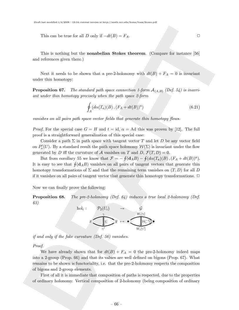
Draft last modified 1/4/2008 – 13:14; current version at http://math.ucr.edu/home/baez/2conn.pdf
DR
AFT
This can be true for all D only if −dt(B) = FA. 2
This is nothing but the nonabelian Stokes theorem. (Compare for instance [56]
and references given there.)
Next it needs to be shown that a pre-2-holonomy with dt(B) + FA = 0 is invariant
under thin homotopy:
Proposition 67. The standard path space connection 1-form A(A,B) (Def. 54) is inavri-
ant under thin homotopy precisely when the path space 2-form
∮
A(dα(Ta)(B) , (FA + dt(B))a) (6.21)
vanishes on all pairs path space vector fields that generate thin homotopy flows.
Proof. For the special case G = H and t = id, α = Ad this was proven by [12]. The full
proof is a straightforward generalization of this special case:
Consider a path Σ in path space with tangent vector T and let D be any vector field
on P ts(U). By a standard result the path space holonomy W(Σ) is invariant under the flow
generated by D iff the curvature of A vanishes on T and D, F(T,D) = 0.
But from corollary 55 we know that F = −∮
(dAB) −∮
(dα(Ta)(B) , (FA + dt(B))a).
It is easy to see that∮
(dAB) vanishes on all pairs of tangent vectors that generate thin
homotopy transformations of Σ and that the remaining term vanishes on (T,D) for all D
if it vanishes on all pairs of tangent vector that generate thin homotopy transformations. 2
Now we can finally prove the following:
Proposition 68. The pre-2-holonomy (Def. 64) induces a true local 2-holonomy (Def.
63)
holi : P2(Ui) → G
x
γ
%%
γ′
99Σ
y 7→ •Wi[γ]
%%
Wi[γ′]
99W−1i (Σ)
•
if and only if the fake curvature (Def. 56) vanishes.
Proof.
We have already shown that for dt(B) + FA = 0 the pre-2-holonomy indeed maps
into a 2-group (Prop. 66) and that its values are well defined on bigons (Prop. 67). What
remains to be shown is functoriality, i.e. that the pre-2-holonomy respects the composition
of bigons and 2-group elements.
First of all it is immediate that composition of paths is respected, due to the properties
of ordinary holonomy. Vertical composition of 2-holonomy (being composition of ordinary
– 66 –
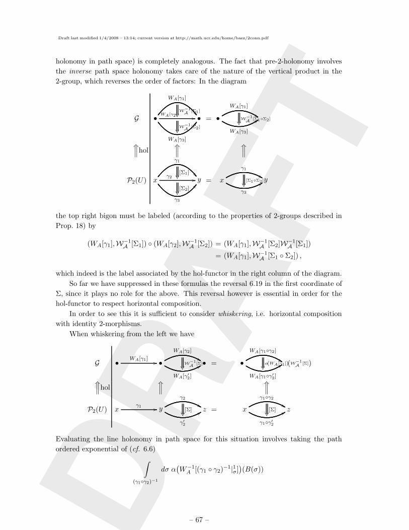
Draft last modified 1/4/2008 – 13:14; current version at http://math.ucr.edu/home/baez/2conn.pdf
DR
AFT
holonomy in path space) is completely analogous. The fact that pre-2-holonomy involves
the inverse path space holonomy takes care of the nature of the vertical product in the
2-group, which reverses the order of factors: In the diagram
G •
WA[γ1]
WA[γ2] //W−1A [Σ1]
WA[γ3]
CCW−1A [Σ2]
• = •WA[γ1]
$$
WA[γ3]
::W−1A [Σ1Σ2]
~wwhol~ww
~ww
P2(U) x
γ1
γ2 //[Σ1]
γ3
BB[Σ2]
y = x
γ1
%%
γ3
99[Σ1Σ2]
y
the top right bigon must be labeled (according to the properties of 2-groups described in
Prop. 18) by
(WA[γ1],W−1A [Σ1]) (WA[γ2],W−1
A [Σ2]) = (WA[γ1],W−1A [Σ2]W−1
A [Σ1])
= (WA[γ1],W−1A [Σ1 Σ2]) ,
which indeed is the label associated by the hol-functor in the right column of the diagram.
So far we have suppressed in these formulas the reversal 6.19 in the first coordinate of
Σ, since it plays no role for the above. This reversal however is essential in order for the
hol-functor to respect horizontal composition.
In order to see this it is sufficient to consider whiskering, i.e. horizontal composition
with identity 2-morphisms.
When whiskering from the left we have
G • WA[γ1] // •WA[γ2]
%%
WA[γ′2]
99W−1A [Σ]
• = •
WA[γ1γ2]
$$
WA[γ1γ′2]
::α(WA[γ1])(W−1A [Σ])
~wwhol~ww
~ww
P2(U) xγ1 // y
γ2
%%
γ′2
99[Σ]
z = x
γ1γ2
&&
γ1γ′2
88[Σ]
z
Evaluating the line holonomy in path space for this situation involves taking the path
ordered exponential of (cf. 6.6)
∫
(γ1γ2)−1
dσ α(W−1A [(γ1 γ2)−1|1σ]
)(B(σ))
– 67 –
Draft last modified 1/4/2008 – 13:14; current version at http://math.ucr.edu/home/baez/2conn.pdf
DR
AFT
evaluated on the tangent vector to the whiskered Σ. Since this vanishes on γ1 and using
the reparameterization invariance of WA the above equals
· · · = α(WA[γ1])
∫
γ−12
dσ α(W−1A [γ−1
2 |1σ])(B(σ))
.
Hence the above diagram does commute. In this computation the path reversal is essential,
which of course is related to our convention that parallel transport be to the point with
parameter σ = 1. A simple plausibility argument for this was given at the beginning of
§6.3.
Finally, whiskering to the right is trivial, since we can simply use reparametrization
invariance to obtain∫
(γ1γ2)−1
dσ α(WA[(γ1 γ2)−1|1σ]
)(B(σ)) =
∫
γ−11
dσ α(WA[γ−1
1 |σ1 ])(B(σ)) ,
because for right whiskers the integrand vanishes on γ2.
Since general horizontal composition is obtained by first whiskering and then compos-
ing vertically, this also proves that the hol-functor respects general horizontal composition.
In summary, this shows that a pre-2-holonomy with vanishing fake curvature (Def. 56)
dt(B) +FA = 0 defines a 2-functor hol:P2(U)→ G and hence a local strict 2-holonomy. 2
– 68 –
Draft last modified 1/4/2008 – 13:14; current version at http://math.ucr.edu/home/baez/2conn.pdf
DR
AFT
7. Appendix: Smooth Spaces
It is a sad fact of life that the category of finite-dimensional smooth manifolds Diff is not
closed under many useful constructions. For example, a subspace or quotient space of a
manifold is usually not a manifold, nor is the space of smooth maps from one manifold to
another. Various approaches to remedying this problem have been proposed; here we use
the last of several variants proposed by Chen [33, 34] in his work on path integrals.
In what follows, we use convex set to mean a convex subset of Rn, where n is arbitrary
(not fixed). Any convex set inherits a topology from its inclusion in Rn. We say a map f
between convex sets is smooth if arbitrarily high derivatives of f exist and are continuous,
using the usual definition of derivative as a limit of a quotient.
Definition 69. A smooth space is a set X equipped with, for each convex set C, a
collection of functions φ:C → X called plots in X, such that:
1. If φ:C → X is a plot in X, and f :C ′ → C is a smooth map between convex sets,
then φ f is a plot in X,
2. If iα:Cα → C is an open cover of a convex set C by convex subsets Cα, and φ:C → X
has the property that φ iα is a plot in X for all α, then φ is a plot in X.
3. Every map from a point to X is a plot in X.
Definition 70. A smooth map from the smooth space X to the smooth space Y is a
map f :X → Y such that for every plot φ in X, φ f is a plot in Y .
It is straightforward to check that there is a category C∞ whose objects are smooth spaces
and whose morphisms are smooth maps.
We make any smooth manifold X into a smooth space by decreeing that the plots
φ:C → X are precisely those maps that are smooth in the usual sense. Given this, one can
check that a map between smooth manifolds is smooth in the sense defined above precisely
when it is smooth in the usual sense, so no confusion arises. In other words, Diff is a full
subcategory of C∞.
The same procedure lets us make any smooth manifold with boundary into a smooth
space. Here we take advantage of plots φ:C → X where C is a half-space.
The one-point space ∗ is a smooth space such that all maps φ:C → ∗ are plots. By
item 3 of Def. 69, all maps from ∗ into a smooth space are smooth. Since smooth maps
are closed under composition, all constant maps between smooth spaces are smooth.
We make a disjoint union X =∐αXα of smooth spaces into a smooth space as follows.
We define a map φ:C → X to be a plot in X if and only if there is a plot ψ:C → Xα such
that φ is ψ composed with the inclusion of Xα in X. One can check that X is indeed a
smooth space and that it is the coproduct in C∞ of the smooth spaces Xα.
We make a Cartesian product X =∏αXα of smooth spaces into a smooth space as
follows. A map φ:C → X is the same as a collection of maps φα:C → Xα, and we decree
– 69 –
Draft last modified 1/4/2008 – 13:14; current version at http://math.ucr.edu/home/baez/2conn.pdf
DR
AFT
φ to be a plot if and only if every map φα is a plot. One can check that X is indeed a
smooth space and that it is the product in the category C∞ of the smooth spaces Xα.
We make a subset X of a smooth space Y into a smooth space as follows. We define
φ:C → X to be a plot if and only its composite with the inclusion i:X → Y is a plot in Y .
One can check that X is indeed a smooth space. Note also that the inclusion i is smooth.
We make a quotient space X of a smooth space Y into a smooth space as follows.
Suppose ∼ is an equivalence relation on Y . As a set, X will be just the usual quotient
Y/ ∼. Let j:Y → X stand for the quotient map. We make X into a smooth space by
decreeing that φ:C → X is a plot iff there is an open cover of C by convex sets, iαCα → C,
such that for every α the map φ iα is of the form j φα for some plot φα:Cα → Y . One
can check that X is indeed a smooth space. Note also that the quotient map j:Y → X is
smooth.
This issue arises when defining smooth spaces of thin homotopy classes of paths (Ex-
ample 12) or parametrized bigons (Def. 35)...
Given smooth spaces X and Y , let C∞(X,Y ) be the set of smooth maps from X to
Y . Given a convex set C, we say that a map φ:C → C∞(X,Y ) is a plot if and only if
φ:C ×X → Y is smooth, where we define
φ(c, x) = φ(c)(x)
for all c ∈ C and x ∈ X. One can check that with this definition C∞(X,Y ) is a smooth
space. One can also check that for any smooth space A, a map f :A ×X → Y is smooth
if and only if the corresponding map f :A → X × Y is smooth. So, we have a one-to-one
and onto map:C∞(A×X,Y ) → C∞(A,C∞(X,Y ))
f 7→ f
and one can even check that this map is smooth, with a smooth inverse. CHECK.
We can summarize many of the facts observed so far in the following result, which
actually goes a bit further:
Theorem 71. The category C∞ is complete, cocomplete, and cartesian closed.
Proof. First let us show that C∞ is complete, meaning that every diagram has a limit.
Suppose we have any diagram F :D → C∞. We show this has a limit as follows. First
we take the limit in Set of the underlying diagram of sets and obtain a set limD F . We
then make this into a smooth space by decreeing the set of plots φ:C → limD F to be
limD C∞(C,F ). One can check that this choice satisfies properties 1-3 in Definition Def.
69. Moreover, given a smooth space X, a map f :X → limD F is the same as a collection
of maps fα:X → F (dα) making the obvious triangles commute, where dα are the objects
of D. By definition f is smooth iff for any plot φ in X, f φ is a plot in limD F . This
is equivalent to demanding that for any plot φ in X and any α, fα φ is a plot in F (dα).
This in turn is equivalent to demanding that each map fα is smooth. So, a smooth map
f :X → limD F is the same as a collection of smooth maps fα:X → F (dα) making the
obvious triangles commute. So, limD F is indeed the desired limit.
– 70 –
Draft last modified 1/4/2008 – 13:14; current version at http://math.ucr.edu/home/baez/2conn.pdf
DR
AFT
For colimits we need sheafification...!!!
Then cartesian closedness!!! 2
One can develop the whole theory of bundles, connections, differential forms and so
on for smooth spaces. We only sketch the first few steps, focusing on what we need for
this paper. We define a differential form on a smooth space in terms of its pullbacks along
plots:
Definition 72. A p-form ω on the smooth space X is an assignment of a smooth p-form
ωφ on Rn to each plot φ:Rn → X, satisfying this pullback compatibility condition for
any map f :Rm → Rn:
f∗ωφ = ωφf .
The space of p-forms on X is denoted by Ωp(X).
Proposition 73. Given a smooth map f :X → Y and ω ∈ Ωp(Y ) there is a p-form
f∗ω ∈ Ωp(X) given by
(f∗ω)φ = ωφf
for every plot φ:Rn → X.
We call f ∗ω the pullback of ω along f . Given a differential form ω on X, the forms ωφdefining it turn out to be just its pullbacks along plots:
Proposition 74. Given a plot φ:Rn → X and ω ∈ Ωp(X) we have
φ∗ω = ωφ.
The above definition and results immediately generalize, for instance, to Lie-group-valued
0-forms Ω0(X,G) and to Lie-algebra-valued p-forms Ωp(X, g). An element F ∈ Ω0(X,G)
is the same as a smooth map F :X → G.
Given a smooth space X, we define the tangent space TxX to consist of formal linear
combinations of smooth maps γ: [0, 1] → X with γ(0) = x, modulo the space of formal
linear combinations∑
i ciγi with the property that
∑
i
cid
dtf(γi(t))|t=0 = 0
for all smooth functions f :X → R.
Acknowledgments
We are grateful to Orlando Alvarez, Paolo Aschieri, Toby Bartels, Larry Breen, Dan Chris-
tensen, James Dolan, Jens Fjelstad, Ezra Getzler, Branislav Jurco, Mikhail Kapranov,
Amitabha Lahiri, Thomas Larsson, Hendryk Pfeiffer, and Danny Stevenson for comments
and helpful discussion. Special thanks go to Eric Forgy for preparing the figure on paths
in loop space. The second author was supported by SFB/TR 12.
– 71 –
Draft last modified 1/4/2008 – 13:14; current version at http://math.ucr.edu/home/baez/2conn.pdf
DR
AFT
References
[1] J. C. Baez and J. Dolan, Categorification, in Higher Category Theory, Contemp. Math. 230.
American Mathematical Society, 1998. math.QA/9802029.
[2] J. C. Baez, Higher Yang-Mills theory. hep-th/0206130.
[3] J. C. Baez and A. Lauda, Higher-dimensional algebra V: 2-groups, Theory and Applications
of Categories 12 (2004) 423–491. math.QA/0307200.
[4] J. C. Baez and A. Crans, Higher-dimensional algebra VI: Lie 2-algebras, Theory and
Applications of Categories 12 (2004) 492–528. math.QA/0307263.
[5] J. C. Baez and U. Schreiber, Higher gauge theory. math.DG/0511710.
[6] T. Bartels, Higher gauge theory: 2-bundles. math.CT/0410328.
[7] R. Attal, Combinatorics of non-abelian gerbes with connection and curvature.
math-ph/0203056.
[8] H. Pfeiffer, Higher gauge theory and a non-Abelian generalization of 2-form
electromagnetism, Ann. Phys. (NY) 308 (2003) 447. hep-th/0304074.
[9] F. Girelli and H. Pfeiffer, Higher gauge theory - differential versus integral formulation.
hep-th/0309173.
[10] O. Alvarez, L. Ferreira, and J. Sanchez Guillen, A new approach to integrable theories in any
dimension, Nucl. Phys. B 529 (1998) 689 (1998). hep-th/9710147.
[11] U. Schreiber, Nonabelian 2-forms and loop space connections from 2d SCFT deformations.
hep-th/0407122.
[12] O. Alvarez, 2004. (private communication).
[13] L. Breen and W. Messing, Differential geometry of gerbes. math.AG/0106083.
[14] P. Aschieri, L. Cantini, and B. Jurco, Nonabelian bundle gerbes, their differential geometry
and gauge theory, Commun. Math. Phys. 254 (2005) 367–400 hep-th/0312154.
[15] P. Aschieri and B. Jurco, Gerbes, M5-brane anomalies and E8 gauge theory, J. High Energy
Phys. 10 (2004) 068. hep-th/0409200.
[16] M. Murray, Bundle gerbes. math.DG/9407015.
[17] D. Stevenson, The Geometry of Bundle Gerbes, Ph.D. thesis, University of Adelaide, 2000.
math.DG/0004117.
[18] M. Mackaay and R. Picken, Holonomy and parallel transport for abelian gerbes.
math.DG/0007053.
[19] U. Schreiber, On deformations of 2d SCFTs, J. High Energy Phys. 06 (2004) 058.
hep-th/0401175.
[20] E. Witten, Conformal Field Theory In Four and Six Dimensions, in Topology, Geometry and
Quantum Field Theory, ed. U. Tillmann. Cambridge U. Press, 2004, pp. 405–419. Slides
available at
http://www.maths.ox.ac.uk/notices/events/special/tgqfts/photos/witten/.
[21] B. Eckmann and P. Hilton, Group-like structures in categories, Math. Ann. 145 (1962)
227–255.
– 72 –
Draft last modified 1/4/2008 – 13:14; current version at http://math.ucr.edu/home/baez/2conn.pdf
DR
AFT
[22] M. Forrester-Barker, Group objects and internal categories, math.CT/0212065.
[23] S. Mac Lane, Categories for the Working Mathematician. Springer, 1998.
[24] J.-L. Brylinski, Loop Spaces, Characteristic Classes and Geometric Quantization. Birkhauser,
1993.
[25] S. J. A. Carey and M. Murray, Holonomy on D-branes. hep-th/0204199.
[26] M. Caicedo, I. Martın, and A. Restuccia, Gerbes and duality, Ann. Phys. (NY) 300 (2002)
32. hep-th/0205002.
[27] N. Hitchin, Lectures on special Lagrangian submanifolds. math.DG/9907034.
[28] A. Keurentjes, Flat connections from flat gerbes, Fortschr. Phys. 50 (2002) 916.
hep-th/0201072.
[29] F. W. Lawvere, Functorial Semantics of Algebraic Categories. Ph.D. thesis, Columbia
University, 1963. Available online at
http://www.tac.mta.ca/tac/reprints/articles/5/tr5abs.html.
[30] C. Ehresmann, Introduction to the theory of structured categories. Technical Report, U. of
Kansas at Lawrence, 1966.
[31] F. Borceux, Handbook of Categorical Algebra 1: Basic Category Theory. Cambridge U. Press,
1994.
[32] K. T. Chen, Iterated integrals, fundamental groups and covering spaces, Trans. Amer. Math.
Soc. 206 (1975), 83–98.
[33] K. T. Chen, Iterated path integrals, Bull. Amer. Math. Soc. 83 (1977), 831–879.
[34] K. T. Chen, On differentiable spaces, in Categories in Continuum Physics, eds. F. W.
Lawvere and S. Schanuel, Lecture Notes in Mathematics 1174, Springer, Berlin, 1986, pp.
38-42.
[35] R. Brown and C. B. Spencer, G-groupoids, crossed modules, and the classifying space of a
topological group, Proc. Kon. Akad. v. Wet. 79 (1976), 296–302.
[36] R. Brown, Groupoids and crossed objects in algebraic topology, Homology, Homotopy and
Applications 1 (1999), 1–78. Available online at
http://www.math.rutgers.edu/hha/volumes/1999/volume1-1.htm.
[37] L. Crane and M. D. Sheppeard, 2-Categorical Poincare representations and state sum
applications. math.QA/0306440.
[38] L. Crane and D. Yetter, Measurable categories and 2-groups. math.QA/0305176.
[39] F. Thompson, Introducing quaternionic gerbes. math.DG/0009201.
[40] A. Pressley and G. Segal, Loop Groups. Oxford U. Press, 1986.
[41] J.C. Baez, A. Crans, D. Stevenson and U. Schreiber, From loop groups to 2-groups.
math.QA/0504123.
[42] E. Witten, The index of the Dirac operator in loop space, in Elliptic Curves and Modular
Forms in Algebraic Topology, ed. P. S. Landweber, Lecture Notes in Mathematics 1326,
Springer, Berlin, 1988, pp. 161–181.
– 73 –
Draft last modified 1/4/2008 – 13:14; current version at http://math.ucr.edu/home/baez/2conn.pdf
DR
AFT
[43] S. Stolz and P. Teichner, What is an elliptic object?, in Topology, Geometry and Quantum
Field Theory: Proceedings of the 2002 Oxford Symposium in Honour of the 60th Birthday of
Graeme Segal, ed. U. Tillmann. Cambridge U. Press, Cambridge, 2004.
[44] A. Grothendieck, Pursuing Stacks, 1983. Available online at
http://www.math.jussieu.fr/∼leila/mathtexts.php.
[45] J. Giraud, Cohomologie Non-Abelienne. Springer, 1971.
[46] I. Moerdijk, Introduction to the language of stacks and gerbes. math.AT/0212266.
[47] A. Caray, S. Johnson, M. Murray, D. Stevenson, and B. Wang, Bundle gerbes for
Chern-Simons and Wess-Zumino-Witten theories. math.DG/0410013.
[48] G. Kelly and R. Street, Review of the elements of 2-categories, in Lecture Notes in
Mathematics 420, pp. 75-103. Springer Verlag, 1974.
[49] N. E. Steenrod, The Topology of Fibre Bundles, Princeton U. Press, 1951.
[50] E. Getzler, D. Jones, and S. Petrack, Differential forms on loop spaces and the cyclic bar
complex, Topology 30 (1991), 339–371.
[51] A. Caetano and R. Picken, An axiomatic definition of holonomy, Int. J. Math. 5 (1993),
835–848.
[52] C. Hofman, Nonabelian 2-forms. hep-th/0207017.
[53] I. Chepelev, Non-abelian Wilson surfaces, J. High Energy Phys. 02 (2002) 013.
[54] D. Chatterjee, On Gerbs. PhD thesis, University of Cambridge, 1998. Available online at
http://www.ma.utexas.edu/~hausel/hitchin/hitchinstudents/chatterjee.pdf.
[55] J. Polchinski, String Theory. Cambridge U. Press, 1998.
[56] R. Karp, F. Mansouri, and J. Rno, Product integral formalism and non-abelian Stokes
theorem, J. Math. Phys. 40 (1999) 6033. hep-th/9910173.
– 74 –