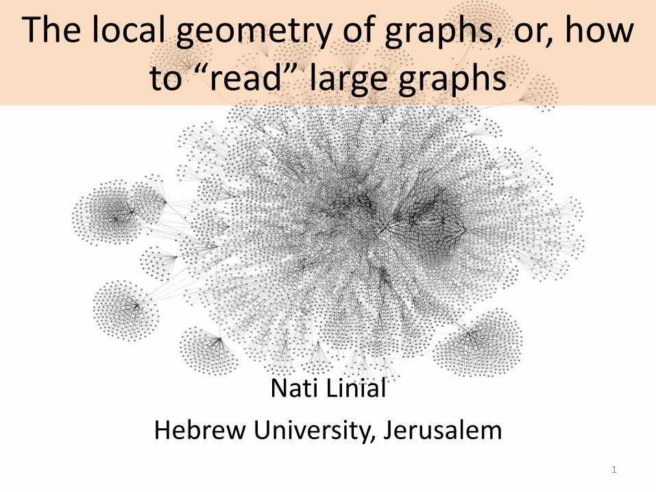
The local geometry of graphs, or, how to “read” large graphs

Nati Linial

Hebrew University, Jerusalem 1

Graphs (aka Networks)

2

Statistics 001

• What do you do with a large collection of numbers that come from some phenomenon or a system which you study?

• The most basic answer: Draw a histogram, look at key parameters – Mean, median, standard deviation…

• Try to fit to known distributions: Normal, Poisson, etc. Estimate key parameters. Draw conclusions on the system at hand.

3

Graph reading 0.001

• We need a parallel methodology when the input is a large graph and not a big pile of numbers.

• Two necessary ingredients for this program: Find out which key parameters should be observed in a big graph (in this talk we discuss one answer to this question).

• Develop a battery of generative models of graphs and methods to recover the appropriate model from the input graph.

4

The main focus of this lecture

• How should we “read/understand” very large graphs? (Possibly graph is so big that it cannot even be stored in our computer’s memory.)

• The approach that we discuss here: Sample small chunks of G (say k vertices at a time) and consider the resulting distribution on k-vertex graphs, to which we refer as a local view of G or the k-profile of G.

5

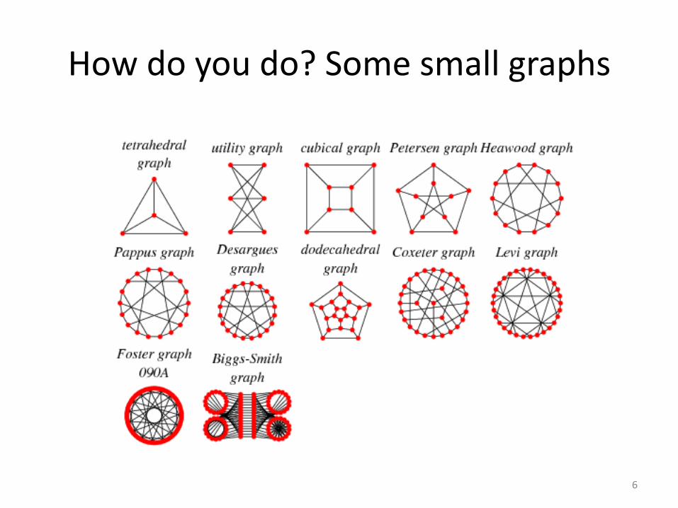
How do you do? Some small graphs

6

Emerging Field: Network Biology

7

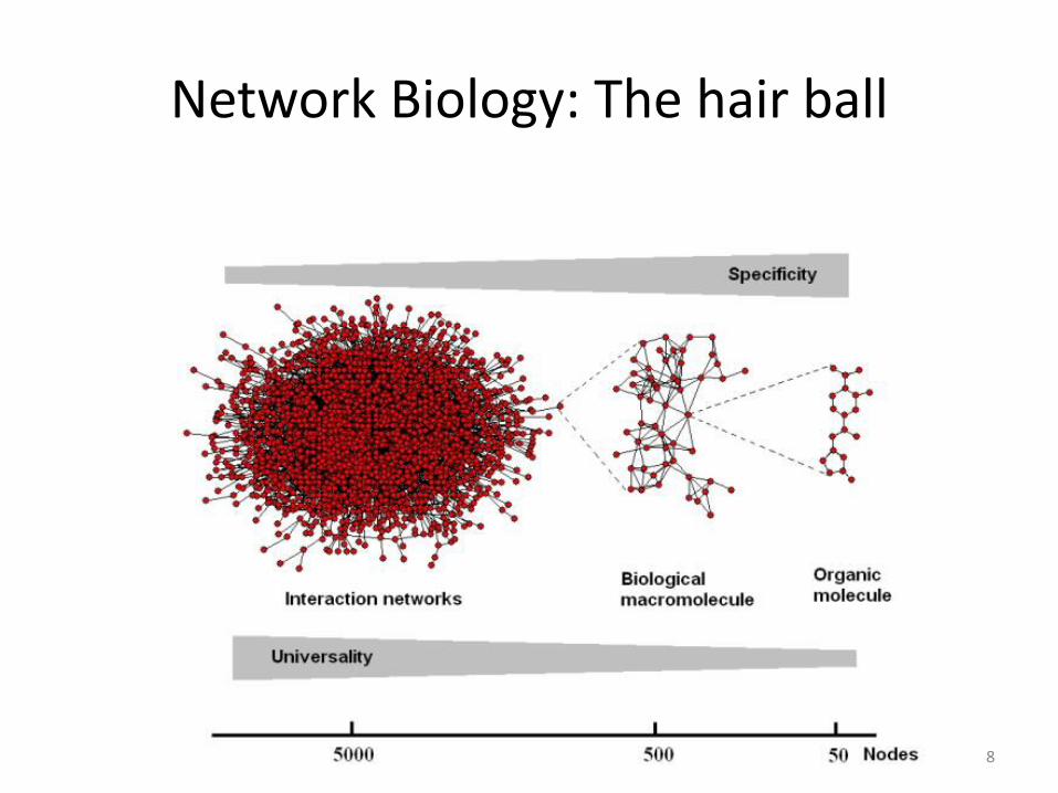
Network Biology: The hair ball

8

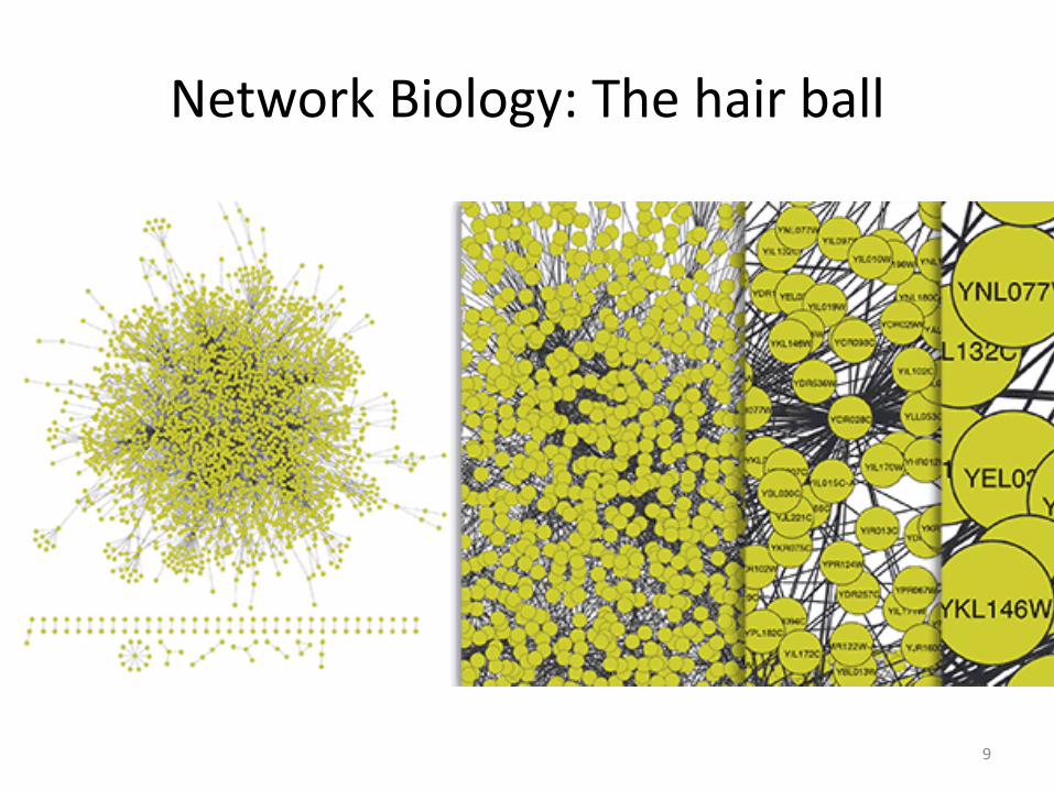
Network Biology: The hair ball

9

The two major questions

• Which local views are possible? (Local graph theory). Namely, which distribution on k-vertex graphs can be obtained as the k-profile of a large graph?

• How are the global properties of G reflected in the local view? (Local-to-global theory). Namely, what large-scale structural conclusions can you infer about G, based on its local view?

10

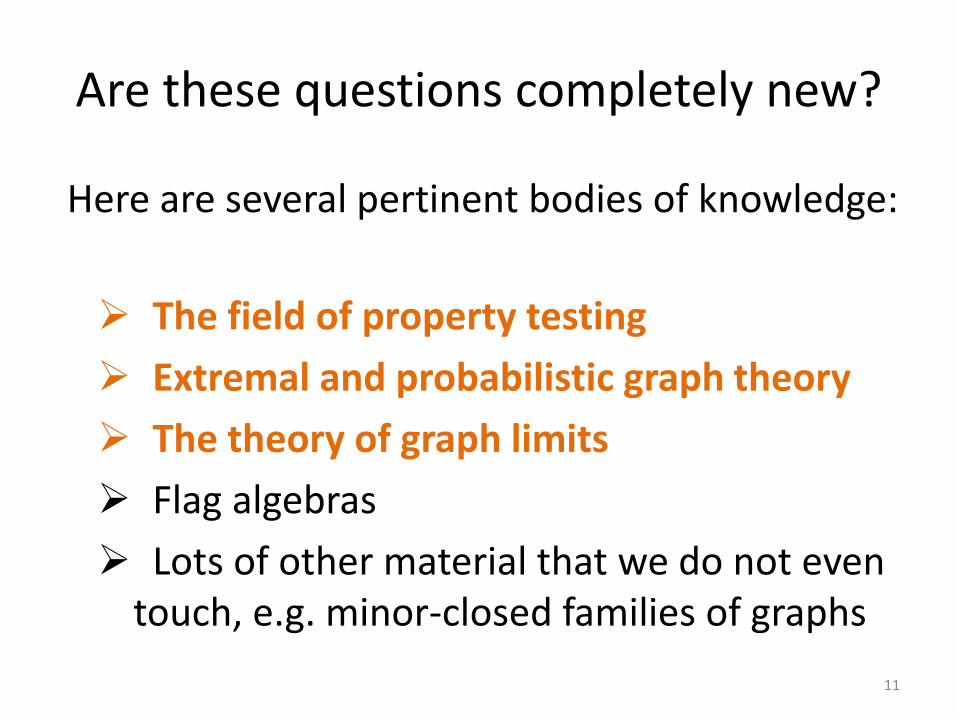
Are these questions completely new?

Here are several pertinent bodies of knowledge:

The field of property testing

Extremal and probabilistic graph theory

The theory of graph limits

Flag algebras

Lots of other material that we do not even touch, e.g. minor-closed families of graphs

11

Are these questions completely new?

Here are several pertinent bodies of knowledge:

The field of property testing

12

Property testing

• We wish to determine whether a huge graph G=(V,E) has some specified graph property P.

For example:

• Is G planar? I.e., can it be drawn in the plane so that no two edges are intersecting?

• Is it 7-colorable? I.e., can the vertices of G be colored by 7 colors so that every two adjacent vertices are colored differently?

13

We seek a super-fast decision method

• We insist that the computation time is bounded by a constant- Independent of the size of G, (which is assumed to be huge).

• Obviously, there are some prices to pay:

A. Our algorithm must be probabilistic, and we must allow for a chance of error.

B. Moreover, we must allow the algorithm to err on ``borderline” instances of the problem.

14

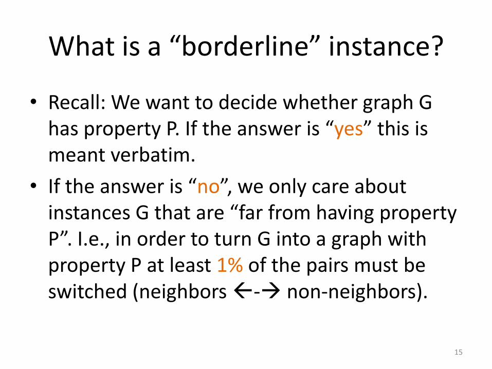
What is a “borderline” instance?

• Recall: We want to decide whether graph G has property P. If the answer is “yes” this is meant verbatim.

• If the answer is “no”, we only care about instances G that are “far from having property P”. I.e., in order to turn G into a graph with property P at least 1% of the pairs must be switched (neighbors - non-neighbors).

15

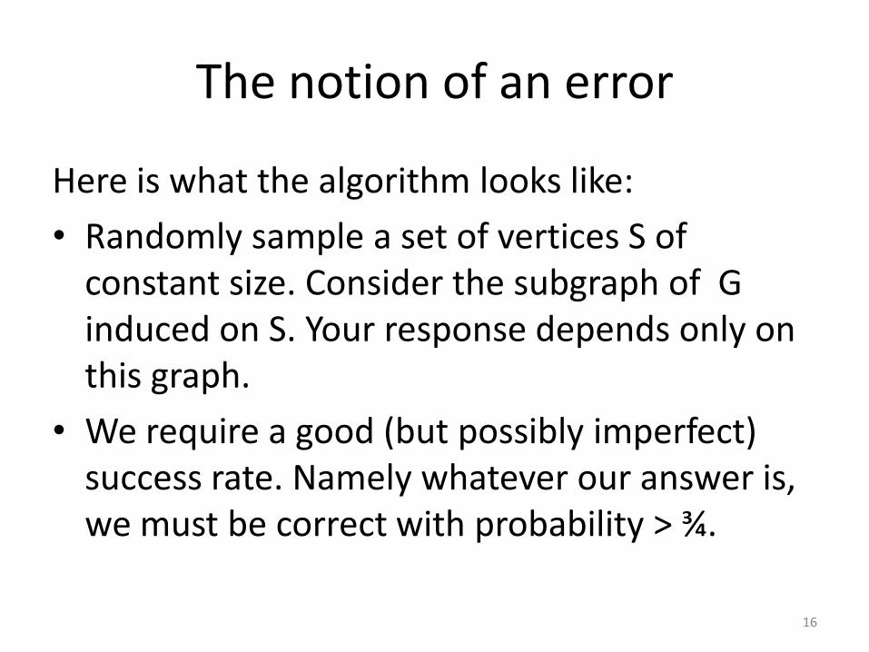
The notion of an error

Here is what the algorithm looks like:

• Randomly sample a set of vertices S of constant size. Consider the subgraph of G induced on S. Your response depends only on this graph.

• We require a good (but possibly imperfect) success rate. Namely whatever our answer is, we must be correct with probability > ¾.

16

A concrete example – Is G bipartite?

• We call G bipartite if its vertices are split in two parts, say L and R and all edges connect an L-vertex to an R-vertex.

• Given access to a huge G we wish to determine whether or not it’s bipartite.

• Note that a subgraph of a bipartite graph is also bipartite, hence the following algorithm suggests itself very naturally.

17

G bipartite?

18

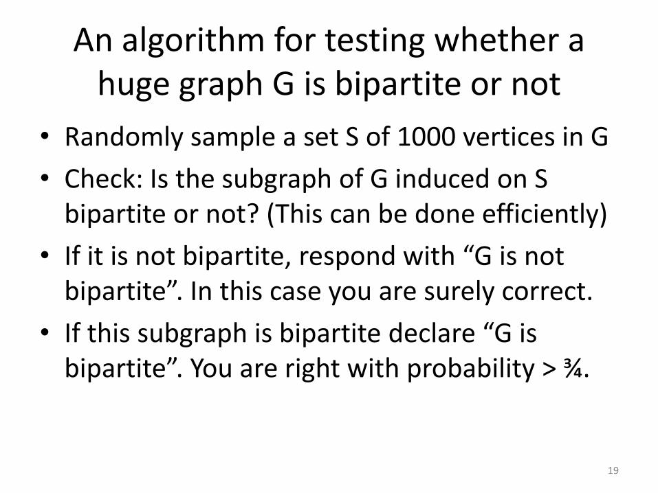
An algorithm for testing whether a huge graph G is bipartite or not

• Randomly sample a set S of 1000 vertices in G

• Check: Is the subgraph of G induced on S bipartite or not? (This can be done efficiently)

• If it is not bipartite, respond with “G is not bipartite”. In this case you are surely correct.

• If this subgraph is bipartite declare “G is bipartite”. You are right with probability > ¾.

19

The crux of the matter

The last statement is quite a nontrivial theorem. It says something like:

•If a graph is 0.01-far from being bipartite, then with probability > 3/4 a randomly chosen set of 1000 vertices will reveal it. •The mavens among you know that there is some statement with Ɛ and δ hiding here, but we will skip such complications 20

In other words

• Let B and F be two huge graphs. B is Bipartite and F is 0.01-Far from being bipartite.

• Consider two distributions on 1000-vertex graphs: The one that comes from local samples of B vs. the same from F.

• The theorem says that these distributions are very different. In the B-distribution all 1000-vertx graph are bipartite, whereas in the F-distribution at most ¼ are bipartite.

21

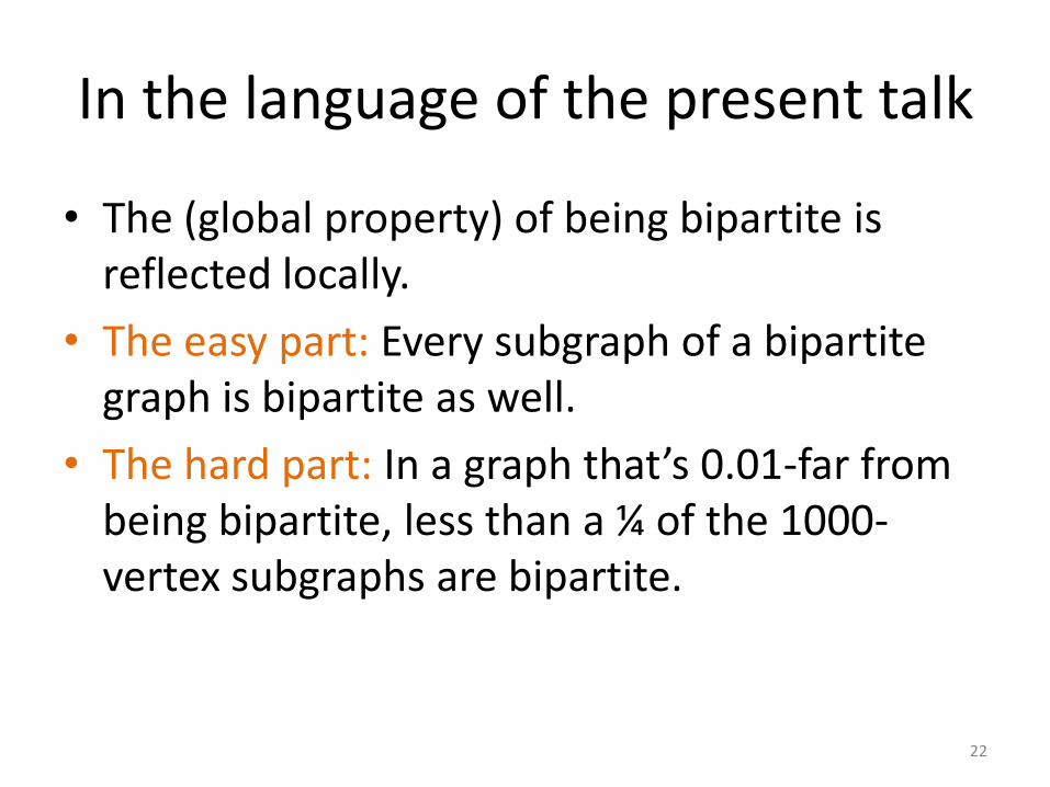
In the language of the present talk

• The (global property) of being bipartite is reflected locally.

• The easy part: Every subgraph of a bipartite graph is bipartite as well.

• The hard part: In a graph that’s 0.01-far from being bipartite, less than a ¼ of the 1000-vertex subgraphs are bipartite.

22

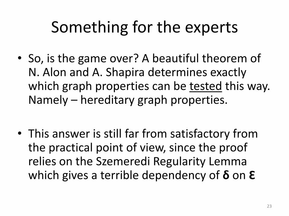
Something for the experts

• So, is the game over? A beautiful theorem of N. Alon and A. Shapira determines exactly which graph properties can be tested this way. Namely – hereditary graph properties.

• This answer is still far from satisfactory from the practical point of view, since the proof relies on the Szemeredi Regularity Lemma which gives a terrible dependency of δ on Ɛ

23

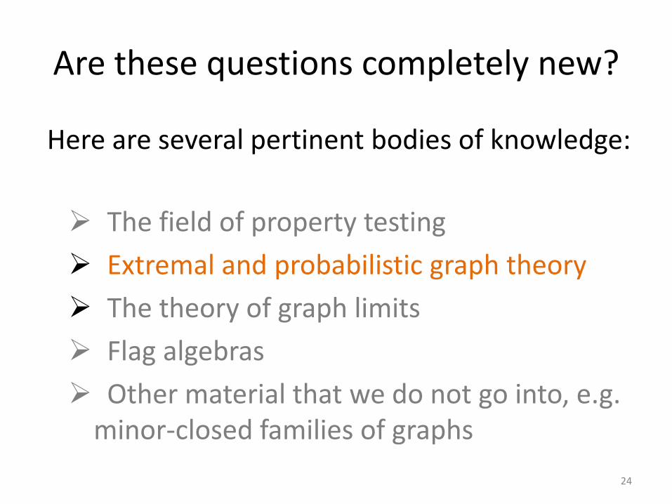
Are these questions completely new?

Here are several pertinent bodies of knowledge:

The field of property testing

Extremal and probabilistic graph theory

The theory of graph limits

Flag algebras

Other material that we do not go into, e.g. minor-closed families of graphs

24

Extremal graph theory - A parent of local graph theory

• A very intuitive thought: A graph with many edges must contain dense sets of vertices.

25

Extremal graph theory - A parent of local graph theory

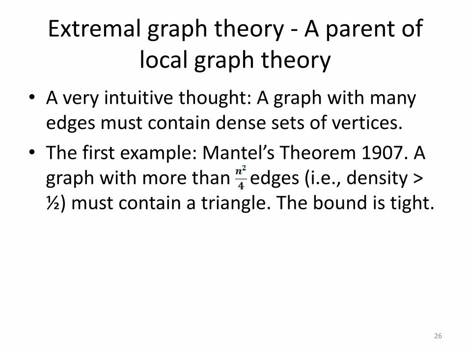
• A very intuitive thought: A graph with many edges must contain dense sets of vertices.

• The first example: Mantel’s Theorem 1907. A graph with more than edges (i.e., density > ½) must contain a triangle. The bound is tight.

26

The grandfather of extremal graph theory

• Turan’s Theorem 1941: A graph with density >(r-2)/(r-1) must contain a complete graph on r vertices. The bound is tight.

27

The density of large H-free graphs

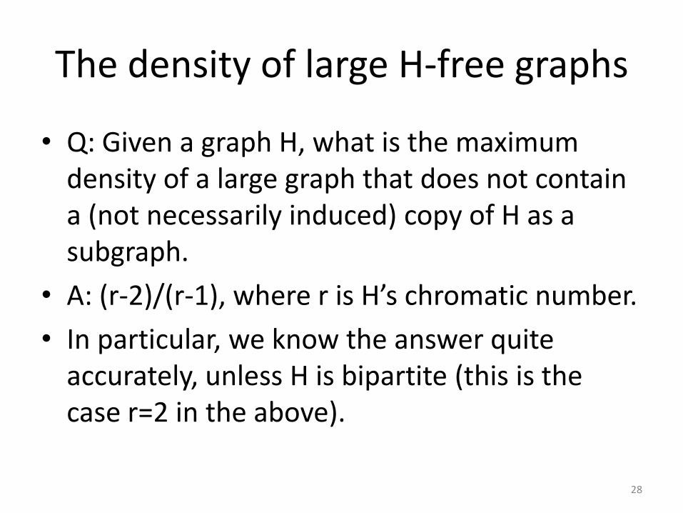
• Q: Given a graph H, what is the maximum density of a large graph that does not contain a (not necessarily induced) copy of H as a subgraph.

• A: (r-2)/(r-1), where r is H’s chromatic number.

• In particular, we know the answer quite accurately, unless H is bipartite (this is the case r=2 in the above).

28

One success with a bipartite H – The case of the 4-cycle

• The largest number of edges in an n-vertex graph that contains no 4-cycle (whether induced or not) is

29

Back to “How to read large graphs ?”

• In statistics we see a bunch of real numbers and we wish to say something worthwhile on the domain from which these numbers came.

30

Back to “How to read large graphs ?”

• In statistics we see a bunch of real numbers and we wish to say something worthwhile on the domain from which these numbers came.

• We realize that the (“empirical”) distribution of the given sample resembles a known distribution (e.g., Normal, Poisson, Gamma…). We estimate the relevant parameters and try to associate with the relevant domain.

31

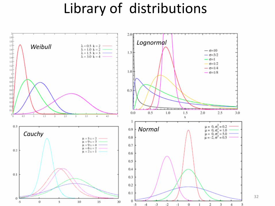
Library of distributions

Normal Cauchy

Lognormal Weibull

32

An analog paradigm for graphs

In order to “read” a large graph G, we:

1. Consider models for generating graphs. 2. Find the best fit among these models. 3. Estimate the relevant parameters. 4. Draw conclusions on the source of the data. We seek to develop the infrastructure that’s needed to make this methodology work.

33

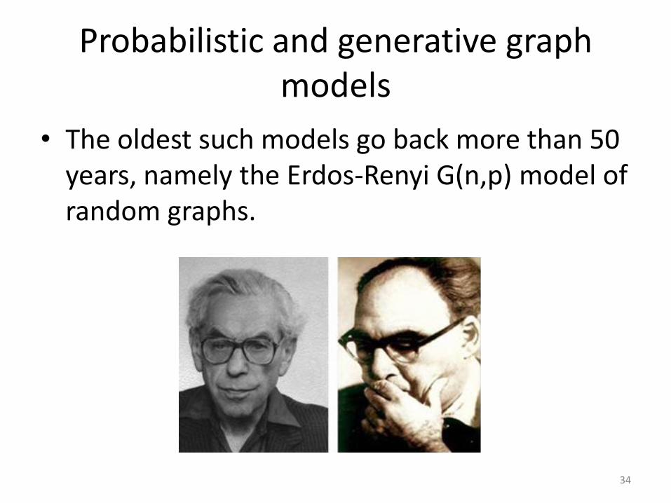
Probabilistic and generative graph models

• The oldest such models go back more than 50 years, namely the Erdos-Renyi G(n,p) model of random graphs.

34

The G(n,p) model

• Here n is an integer (which we normally take to be large – We are interested in the asymptotic theory) and the parameter 1>p>0.

• We start with n vertices. Independently, for each pair of vertices xy we put in the edge xy.

35

G(n,p) theory

• This is the simplest, most basic and most thoroughly understood theory of random graphs. Very flexible and easy to investigate.

• It taught us many previously unexpected things about large graphs.

• On the other hand it’s very simplistic, and too restricted for the purpose of modeling large real-life networks.

36

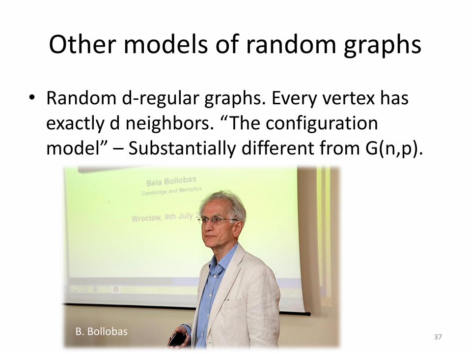
Other models of random graphs

• Random d-regular graphs. Every vertex has exactly d neighbors. “The configuration model” – Substantially different from G(n,p).

B. Bollobas 37

Other models of random graphs • Percolation models – Start from a d-dimensional

grid, maintain edges independently with probability p. Originated in statistical mechanics

• Random graph covers (aka “random lifts”). A model of graph that combines deterministic with stochastic ingredients.

38

Generative models

• Preferential attachment models: An evolving graph model. Start with a seed graph. At each step add a new vertex that becomes a neighbor of a random subset of the earlier vertices with a preference towards high-degree vertices.

• Models of growth + mutations. E.g., a random vertex spawns a ``clone” that slightly ``mutates” the neighbor set of the original vertex.

39

Back to local graph theory: Ramsey’s theorem

• “Total chaos is impossible”. This is a fundamental principle in combinatorics and in many other mathematical areas.

• In particular, every large graph must contain a substantially large homogeneous set, i.e., a clique (a subgraph in which every two vertices are adjacent) or an anti-clique (a set of vertices with no edges).

40

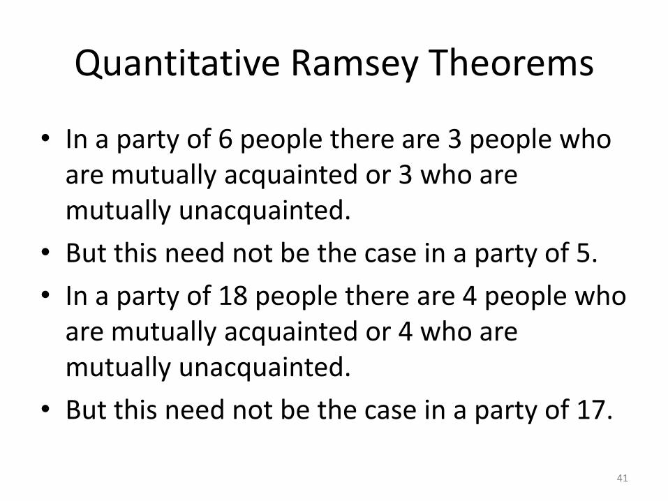
Quantitative Ramsey Theorems

• In a party of 6 people there are 3 people who are mutually acquainted or 3 who are mutually unacquainted.

• But this need not be the case in a party of 5.

• In a party of 18 people there are 4 people who are mutually acquainted or 4 who are mutually unacquainted.

• But this need not be the case in a party of 17.

41

Ramsey’s Theorem R(3,3)>5

42

Ramsey’s Theorem R(3,3)=6

43

Ramsey’s Theorem R(4,4)>17

44

Asymptotic Ramsey Theorem

• Every n-vertex graph must contain a homogenous set of > ½ log n vertices.

• There are n-vertex graphs with no homogenous set of 2 log n vertices. In fact a random G(n, ½) graph has this property.

• The birth of the probabilistic method.

45

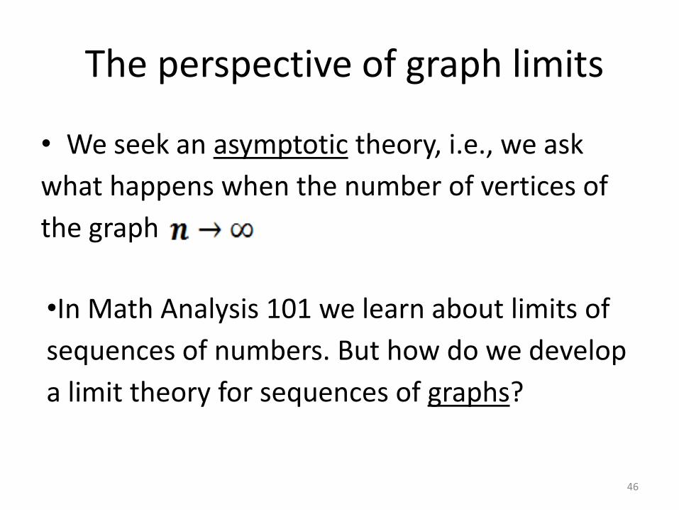
The perspective of graph limits

• We seek an asymptotic theory, i.e., we ask

what happens when the number of vertices of

the graph

•In Math Analysis 101 we learn about limits of

sequences of numbers. But how do we develop

a limit theory for sequences of graphs?

46

It is well known…

• If you want a limit theory, all you need is a notion of distance (``a metric”) d(x,y). You declare that the sequence converges if all distances are arbitrarily small provided m and n are large enough. (Remember ``Cauchy sequences”?)

So, in order to define graph limits all we need is a way to quantify the distance between two graphs G and H.

47

• So, how do you measure the distance between two graphs G and H?

• We say that G and H are close if it’s possible to chop the vertex sets of both G and of H into N (large integer) equal parts each, so that the following holds: For every i<j, the density of the edge set between the i-th and the j-th part in G and in H are nearly equal.

• In words: There is an N-vertex edge-weighted graph that approximates well both G and H.

48

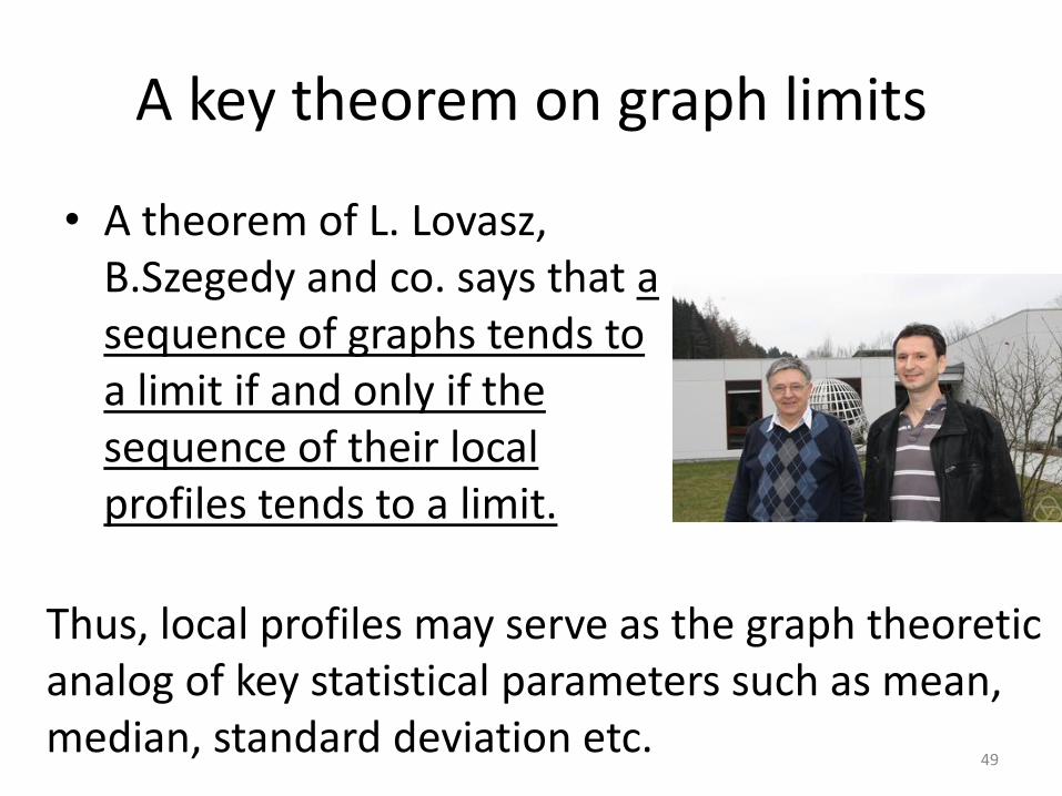
A key theorem on graph limits

• A theorem of L. Lovasz, B.Szegedy and co. says that a sequence of graphs tends to a limit if and only if the sequence of their local profiles tends to a limit.

Thus, local profiles may serve as the graph theoretic analog of key statistical parameters such as mean, median, standard deviation etc.

49

3-profiles

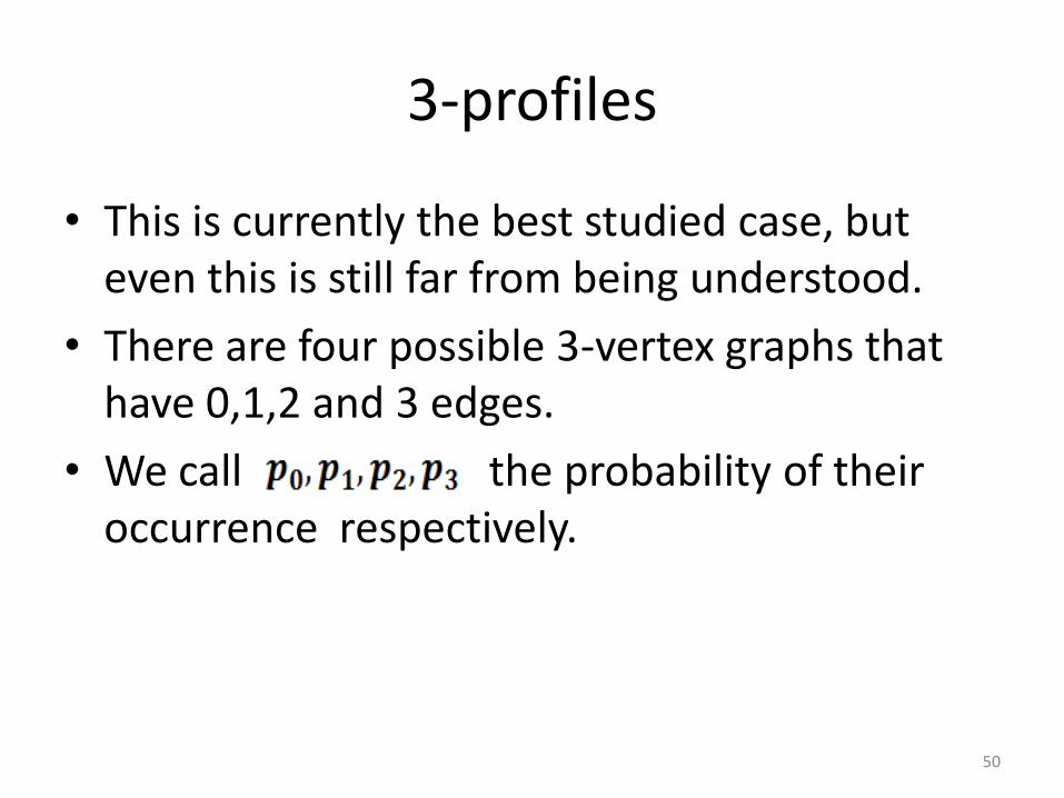
• This is currently the best studied case, but even this is still far from being understood.

• There are four possible 3-vertex graphs that have 0,1,2 and 3 edges.

• We call the probability of their occurrence respectively.

50

3-profiles

• This is currently the best studied case, but even this is still far from being understood.

• There are four possible 3-vertex graphs that have 0,1,2 and 3 edges. We call the probability of their occurrence respectively.

• Goodman’s inequality:

• With Huang, Naves, Peled and Sudakov we proved The bound is tight.

P0 P1 P2 P3

51

Paul Erdos and the Martians

52

But even 4-profiles are still completely mysterious to us

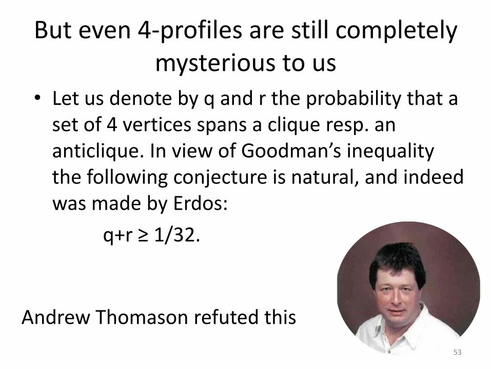
• Let us denote by q and r the probability that a set of 4 vertices spans a clique resp. an anticlique. In view of Goodman’s inequality the following conjecture is natural, and indeed was made by Erdos:

q+r ≥ 1/32.

Andrew Thomason refuted this

53

A word on flag algebras

• Recall Turan’s theorem for triangles: A graph with density > ½ must contain a triangle.

54

A word on flag algebras

• Recall Turan’s theorem for triangles: A graph with density > ½ must contain a triangle.

• So, e.g., does a graph with density 0.77 necessarily contain many triangles? In words, how small can be if the density=0.77?

55

A word on flag algebras

• Recall Turan’s theorem for triangles: A graph with density > ½ must contain a triangle.

• So, e.g., does a graph with density 0.77 necessarily contain many triangles? In words, how small can be if the density=0.77?

• Natural guess: The extreme example for Turan is a bipartite graph with two equal parts. So, try a 5-partite graphs with 4 equal and one smaller parts to achieve right density.

56

• This was conjectured to be answer, but was open for many years, until proved correct by A. Razborov.

57

• His main idea: Rather than seek linear inequalities, find quadratic inequalities. Specifically, he has a method to show that certain matrices which capture some of the local structure of graphs are positive semidefinite.

• Computer assisted proofs.

58

That’s all folks

59

• We already saw the simple observation that a bipartite graph contains no triangles.

• For us, these are ``uninteresting” triangle-free graphs.

• What complicates matters is a theorem of Erdos, Kleitman and Rothschild almost all triangle-free graphs are bipartite.

• So how can we sample ``interesting” triangle-free graphs?

What does a typical triangle-free graph look like?

60

The triangle-free graph process

• Tom Bohman managed to analyze this process, using Wormald’s method of differential equations.

• He showed that almost surely this process terminates with a graph that is tight in terms of Ramsey’s Theorem.

61

The triangle-free graph process

• Erdos and Renyi have introduced a close relative of the G(n,p) model, called ``the evolution of random graph”.

• This model starts with n vertices and no edges. Sequentially at each step a new random edge is added.

• The triangle-free process does the same, except that if a prospective new edges closes a triangle, it’s discarded.

62

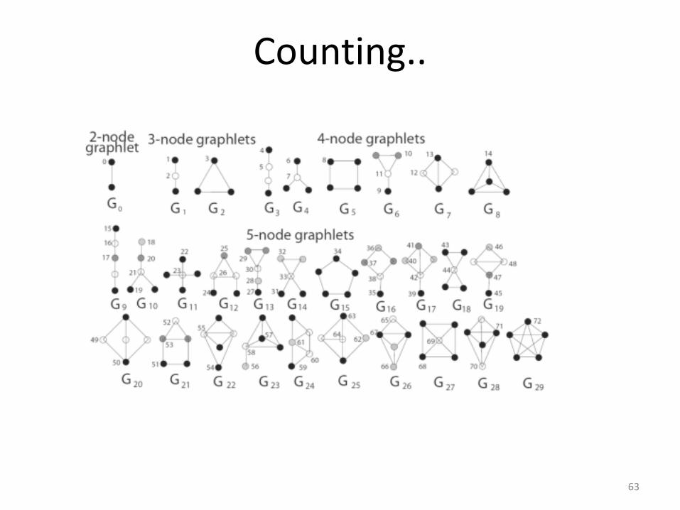
Counting..

63