1

Human Capital, Technology Adoption and Firm Performance:

Impacts of China's Higher Education Expansion in the Late 1990s

(Human Capital, Technology, Firm Performance)

Yi Che

Lei Zhang1

March 2017

Abstract

We exploit a policy-induced exogenous surge in China’s college-educated workforce that started

in 2003 to identify the impact of human capital on productivity. Using a difference-in-differences

estimation strategy, we find that industries using more human-capital intensive technologies

experienced a larger gain in total factor productivity after 2003 than they did in prior years.

Exploring the pathways from human capital increases to TFP growth, we find that these

industries also accelerated new technology adoption, as reflected in the importation of advanced

capital goods, R&D expenditure, and capital intensity, as well as employment of more highly

skilled individuals. The productivity gains were weaker for domestic private firms than for

foreign-owned firms.

Key words: human capital; technology adoption; total factor productivity; higher education

expansion; China

JEL Code: I25; J24; O15; O33

1 Corresponding author: Lei Zhang, Antai College of Economics and Management, Shanghai Jiao Tong University, 1954 Huashan Road, Shanghai 200030, China. Email: zlei89@gmail.com.

This paper benefits from early discussions with Lixin Colin Xu. We thank Alan Auerbach, Stacey Chen, William Dougan, Eric Hanushek, Christos Makridis, Hao Shi, Robert Willis, and seminar participants at Fudan University, Peking University, Renmin University of China, NEUDC, SOLE, and WEAI for helpful comments and suggestions and Ye Peng, Zhaoneng Yuan, Zhicheng Zhang, and Jing Zhao for valuable research assistance. Part of the work was completed when Lei Zhang was visiting the Robert D. Burch Center for Tax Policy and Public Finance at UC-Berkeley. Lei Zhang acknowledges financial support from Shanghai Pujiang Talent Grant No. 14PJC072. Yi Che acknowledges financial support from Shanghai Pujiang Program (16PJC048).

2

Human capital plays an indispensable role in productivity improvement and long-term growth. In

developing countries, the lack of skilled labor force poses a major barrier to firms’ adoption of

frontier technologies that are developed in more advanced economies (Nelson and Phelps, 1966;

Caselli, 1999; Acemoglu and Zilibotti, 2001; Caselli and Coleman 2006), thereby restraining

efficiency in production. Increases in skilled labor force in a developing country facilitate firms’

adoption of frontier technology and hence raise productivity.

We investigate this hypothesis taking advantage of a unique natural experiment in China

that substantially expanded college access for high-school graduates starting in 1999, generating

a subsequent surge in college-educated workers starting in 2003. This higher-education

expansion policy was implemented as part of the economic stimulus plan adopted in the

aftermath of the 1997 Asian financial crisis. The centrally-planned nature of the Chinese higher

education system means that the ensuing dramatic increase in the college-educated workforce

was exogenous to China's economic growth trend, thereby providing a unique opportunity to

identify the impact of human capital on technology adoption and productivity. We estimate this

impact using a unique panel dataset of privately-owned manufacturing firms for 1998-2007.

Using a generalised difference-in-differences (DD) model, we compare the outcomes of firms in

more human-capital-intensive industries with those of firms in less human-capital-intensive

industries before and after the sharp increase in the college-educated labor force. The DD model

allows us to eliminate macroeconomic shocks with industry- and year-fixed effects. We conduct

numerous robustness checks to further deal with potential confounding influences.

We find a significantly larger increase in productivity (measured by total factor

productivity, TFP) of firms in more human-capital intensive industries in the post-2003 years

relative to 1998-2002. Dynamic analysis shows that, prior to 2003, TFP of firms in all industries

3

followed the same trend, but between 2002 and 2003 there was a much larger increase in TFP of

firms in more human-capital-intensive industries. Relative TFP stays at this higher level for the

rest of the sample period. Robustness checks indicate that the results are not driven by China's

accession to the World Trade Organization (WTO) at the end of 2001 or other concurrent

macroeconomic shocks, agglomeration effects in specific cities, spillover effects from the reform

of state-owned firms, or particular subsets of firms.

There are, however, significant differences between the productivity growth trends of

domestic private firms and foreign-owned firms. The relative gains in TFP by domestic private

firms in more human-capital intensive industries are much smaller than those of foreign firms:

While the TFP of foreign firms in more human capital intensive industries grew relatively faster

in the entire post-2003 period, the productivity gains of domestic private firms vanished towards

the end of the sample period. This pattern suggests the existence of severe constraints faced by

domestic private firms in taking advantage of the increased supply of skilled workers. It also

suggests that improvements in credit, taxation, and labor market policies could play important

roles in overcoming those constraints.

Overall, relative to 1998-2002 firms in more human-capital intensive industries exhibit

larger increases post 2003 in imports of advanced capital goods, capital intensity, R&D

expenditure, and new product sales. As a result, they have become relatively more important in

the manufacturing sector, with larger increases in value added, output, and capital stock. These

increases have been accompanied by changes in the composition of employment: between 1995

and 2004 there was a relatively larger increase in the employment of more educated workers, as

well as workers with the job titles of engineer and technician, in more human-capital intensive

industries.

4

This paper contributes to the empirical literature on the role of human capital in

technology diffusion and economic growth. Benhabib and Spiegel (2005) demonstrate via cross-

country regressions that years of schooling are positively correlated with a country’s rate of

catch-up to leader nations' total factor productivity. Eaton and Kortum (1996), Coe et al. (1997),

Xu and Wang (1999), Xu (2000), and Caselli and Coleman (2001) document that technology

diffusion through imports of capital goods or foreign direct investment tends to increase the level

of a country's human capital. These studies however are beset by problems of human-capital

endogeneity and mismeasurement (Bils and Klenow, 2000; Krueger and Lindahl, 2001;

Hanushek and Kim, 2000). More recent studies, such as Becker et al. (2011), Lewis (2011),

Hornung (2014), and Squicciarini and Voigtländer (2015) use a case study or a historical natural

experiment to generate exogenous variation in the quantity of human capital and examine its role

in facilitating technology adoption in specific industries and countries at particular times.

Methodologically, this paper is in the same vein as these recent studies, where causal

identification is achieved by using an exogenous shock to the stock of human capital induced by

a natural experiment. Additionally, our focus on college graduates provides a more suitable

measure of human capital in the context of technology adoption. The rich information from

multiple firm-level databases also allows us to explore thoroughly the links among human capital,

technology adoption, and productivity in a wider range of industries. These are rarely done in a

contemporary developing-country setting.

This paper is also related to the literature on the impact of schooling expansion in

developing countries. Most of these studies focus on the private returns to individuals who

receive more education due to the expansion. Duflo (2001) finds that a large-scale primary

school construction program in Indonesia in the 1970s led to increases in years of schooling and

5

earnings for affected cohorts. Li et al. (2014) study the same higher education expansion policy

as our paper and find negative effects on employment of the cohorts of college graduates

affected by the policy. This paper complements and extends existing studies by investigating the

externality of education expansion, i.e., its impacts on firm productivity and technology adoption.

The paper is organised as follows. Section 2 briefly describes the evolution of the

Chinese higher education sector and, in particular, events surrounding the expansion beginning

in 1999. Section 3 presents the theory underlying the empirical analysis and outlines the

estimation strategy. Section 4 describes data sources and summary statistics. Sections 5 and 6

present estimation results on firm productivity, technology adoption, and employment changes.

Section 7 concludes.

1 Background

1.1 Higher Education in China

The central government has been critical in shaping the evolution of China's higher education

(HE) sector since the founding of the People's Republic of China in 1949. In the early 1950s the

HE institutions were nationalised and reorganised following the Soviet model, resulting in a

dozen or so comprehensive universities and a large number of specialised colleges. Under that

model, the central government, based on its economic development plan, makes detailed

admission plans for each department in each university and is responsible for the placement of

all graduates (Min, 2004; Pepper, 1984). All students are admitted through a unified national

college entrance exam (CEE). The HE sector grew steadily in the 1950s, with college enrolment

rate increasing from 0.02% of population in 1949 to 0.07% in 1957 (Appendix Figure A1). This

steady growth trend was disrupted by two abnormal developments. The first was the higher-

education "Great Leap Forward," concurrent with the economic "Great Leap Forward" of 1958

6

to 1961, when the central government initially planned to achieve universal HE access in 15

years, but that initial period was followed by a severe downsizing in the next four years (Wan

2006). The second major event was the Cultural Revolution of 1966 to 1976, which all but

destroyed China's HE system and reduced HE enrolment by 1976 to a level below that of 1957.

The HE sector returned to a steady growth path in 1977. In the 1990s, to improve its

efficiency and its role in local economic development, the central government implemented a

series of reforms of the HE sector. These included more responsibilities of provincial

governments to finance and administer HE institutions, consolidating institutions to take

advantage of economies of scale, substantial tuition payments by college students, and

curriculum reforms to broaden the education of students to make them more adaptable in the

labor market.2

1.2 Higher Education Expansion since 1999

During the 1997 Asian financial crisis the Chinese government maintained the value of the Yuan,

causing a substantial contraction in exports. The resulting economic downturn and increase in

unemployment were compounded by the reforms of the state-owned enterprises (SOEs) that

generate a large number of laid-off workers. Against this backdrop, the Chinese Politburo

adopted the proposal of Mr. Min Tang, then Chief Economist of the Asian Development Bank’s

Beijing office, who proposed in late 1998 to “double college admissions” to stimulate domestic

demand for educational services and hence investment in construction, services, and other related

industries and to postpone high school graduates' entry into the labor market.3

2 The number of majors is reduced from over1400 in the mid-1980s to around 200 in 2003 (Min, 2004).

In January 1999

the Ministry of Education (MOE) announced an admission plan of 1.3 million for 3- and 4-year

3 In a letter written to the central government leaders in November 1998, Mr. Tang proposed an “effective way to stimulate Chinese economy – double the college admission”. The letter was published in a major newspaper on February 19, 1999 (http://finance.sina.com.cn/review/20041023/15201102716.shtml). See also Bai (2006) and Wan (2006) .

7

college programs, a 20% increase over 1998. The following June it revised the admission plan to

1.56 million, an unprecedented increase of 44% over the previous year.4

Annual college admission growth averaged 4.7% between 1995 and 1998, a moderate

growth rate largely to accommodate the predicted demand for skilled labor due to economic

growth, especially demand of the state sector. In sharp contrast, college admissions grew

annually by more than 40% in both1999 and 2000, and by about 20% over the next five years,

before tapering off in 2006 (Figure 1, top panel). By comparison, annual GDP growth rate was

around 10% from 1995 to 2005. Nationwide college enrolment doubled between 1998 and 2001

and quadrupled by 2005 (Figure 1, bottom panel, statistics in Appendix Table A1). The gross

college enrolment rate among 18-22 year-olds increased from 9.8% in 1998 to 24.2% in 2009.

All but very few college students graduate on time, so increased admissions translate into

increased graduates in about 4 years, as shown in Figure 2. Because the goal of the higher

education expansion policy is to stimulate aggregate demand and is not targeted at any particular

sector, the surge in college graduates in the labor force is exogenous to the growth trend of any

particular industry or firm and allows credible identification of the causal relationship between

human capital and firm economic performance.

2 Analytical Framework

2.1 A Descriptive Theory of Human Capital, Technology Adoption, and Productivity Growth

One important reason that firms in less-developed countries have lower productivity than firms

in developed countries is a lack of skilled labor. This may lead to the employment of

technologies inside the frontier or a mismatch between relatively low-skilled workers and

4 "Major Events of Educational Development in 1999", Ministry of Education. URL: http://www.moe.gov.cn/publicfiles/business/htmlfiles/moe/moe_163/200408/3460.html. The continued consolidation of HE institutions and reorganization within universities such as combining small departments and broadening specialties provides the immediate capacity for expansion. Over time many new campuses are constructed. Faculty-student ratio increases from 5 in 1993 to 15 in 2003, following the new MOE standards.

8

frontier technologies that are primarily invented in developed countries to fit their factor

endowments (Acemoglu, 1998; Caselli, 1999; Acemoglu and Zilibotti, 2001; Caselli and

Coleman 2006). When the constraint on the stock of skilled workers is substantially relaxed such

as through a rapid expansion of formal education, firms may be able to adopt new and more

productive technologies, match frontier technologies with more qualified workers, and conduct

their own R&D. All of these activities are likely to lead to higher firm productivity and economic

growth (Temple and Voth, 1998; Fadinger and Fleiss, 2011; Madsen, 2014).

Meanwhile, the world technology frontier does not progress uniformly across industries.

As well documented by Autor et al. (1998), Kahn and Lim (1998), and Goldin and Katz (2008),

technology progresses since the 1970s are skill-biased, which increases the productivity of

workers with higher levels of human capital, such as college graduates, more than those with low

levels of human capital, leading also to faster growth in total factor productivity in more human-

capital intensive industries.

We conducted informal interviews in several domestic private firms in the suburb of

Ningbo in Zhejiang province; their stories bear out the above hypothesis. Two firms

manufacturing electric machinery report that the hiring of more college graduates since the early

2000s has benefitted their bottom line mainly for three reasons. First, because college graduates

are able to read and understand the manuals of delicate tools and computer-automated machines,

in particular those in English, they can operate the equipment more efficiently and cause less

damage to the equipment. They also translate and post the Chinese labels and instructions for key

parts of the equipment, easing the job of other workers. Another advantage emphasised by the

managers is that most of the maintenance and repair work can now be done by the new college-

educated workers themselves in a timely manner rather than having to wait for the suppliers to

9

provide these services. Second, college graduates’ knowledge in technical drawing, circuit

design, and properties of various materials enables them to quickly translate the intuitive ideas

for product improvement of experienced workers and managers into scientific designs and

prototypes. The manager of one firm gave the example of an improved electric stacker designed

within three months by a group of newly-hired college graduates. Third, the hiring of an

increasing number of college graduates allows firms to improve organization and managerial

practices. For example, one firm has adopted the ERP (Enterprise Resource Planning) system.

The other two firms make apparel and simple metal products; their increase in the hiring of

college graduates is quite modest, and these new hires mostly work in marketing and export-

related functions. All firms agree that college graduates are quick learners relative to other

workers.5

2.2 Empirical Framework

However, they all express concerns that college graduates, especially those of elite

universities, are unwilling to take jobs in manufacturing firms, particularly private firms such as

theirs. These are indeed reflected in the heterogeneous estimation results presented in Section 5.4.

Based on the above theoretical analysis and exploiting the exogenous surge in the supply of

skilled labor generated by the HE expansion policy, we conduct our empirical analysis in a

generalised difference-in-differences (DD) framework, in which we compare changes in

performance before and after the HE expansion of firms in more human-capital intensive

industries to that of firms in less human-capital intensive industries. The intuition is illustrated in

Figure 3, where Industries 1, 2, 3 are the high, medium, and low human-capital intensity

5 An alternative view about the role of higher education is that it serves a screening function and selects more capable people. While we are not able to directly test the relative importance of this versus the human capital hypothesis, the examples given by firm managers suggest that a college education does impart useful knowledge and skills to students, which allow them to contribute to the firm productivity. Estimation results reported in Table 10 indicate that graduates in the science and engineering fields contribute the most to the relative TFP growth; suggesting that it is the special knowledge graduates learn in these fields rather than their raw talent that enables them to improve the firm productivity.

10

industries, and the height of each bar indicates firm performance in each industry if the frontier

technology is employed.6

We implement the DD analysis in the following regression equation:

Before the higher-education expansion, Industry 3 is at the frontier

performance level. Due to the lack of skilled labor, Industries 1 and 2 can only reach

performance level A, far below the frontier; the gap is particularly large for Industry 1. The HE

expansion relaxes the skilled-labor constraint and allows firms in Industries 1 and 2 to adopt

more advanced technologies. Firm performance in both industries improves, and the increase is

larger in Industry 1. In short, the DD method estimates the extra performance increase in

Industry 1 relative to that in Industry 2 following the HE expansion.

𝑦𝑖𝑗𝑡 = 𝛼𝑖 + 𝛾𝑡 + 𝛽 ∙ �𝐼𝑛𝑑𝑢𝑠𝑡𝑟𝑦𝐻𝐶𝑗 ∙ 𝑝𝑜𝑠𝑡𝑡� + 𝜑 ∙ 𝑋𝑖𝑗𝑡 + 𝜀𝑖𝑗𝑡, (1)

where 𝑦𝑖𝑗𝑡 is a performance measure for firm i in industry j in year t. 𝐼𝑛𝑑𝑢𝑠𝑡𝑟𝑦𝐻𝐶𝑗 is the human

capital (HC) intensity of industry j, measured by the percentage of workers with a four-year

college education or more in industry j in the U.S. in 1980. The assumption is that, given the

relative flexibility of the U.S. labor market, and the fact that the bulk of new technologies in the

1970s were created in a handful of the world’s richest countries with the U.S. leading the way,

the industry HC intensity in the U.S. reflects the underlying frontier technology of industries in

general. In contrast, a measure based on Chinese industries is likely contaminated by policy

influences and distortions in resource allocation. This strategy is similar to Hsieh and Klenow

(2009), who use the U.S. labor share as a benchmark for Chinese and Indian industries. The

variable 𝑝𝑜𝑠𝑡𝑡 is an indicator equal to 1 for 2003 and later years and 0 for years before 2003,

since 2003 is the first year when students admitted to a 4-year college program in 1999 graduate

and enter the labor market. The coefficient of interest is the estimate on the interaction between

6 The ranking of the industry performance by human capital intensity is a simplification assumption.

11

HC intensity and the post-2003 dummy, β; it measures the extra increase in y after 2003 relative

to prior years for an industry with one percentage point more of college-educated workers. We

expect β to be positive if Chinese firms in more HC-intensive industries catch up more rapidly

when more skilled workers become available.

The vector 𝛼𝑖 is a full set of firm fixed effects to control for firm-specific time-invariant

factors such as managerial ability and connections that may affect a firm’s performance. Thus,

identification of β is based on firms that are in the sample at least once both before and after

2003. This strategy also addresses potential biases in estimation due to firm entry and exit. The

vector 𝛾𝑡 is a full set of year fixed effects to control for nationwide economic shocks or policy

changes that affect all firms similarly such as monetary policy. Other changes in the economy

such as economic openness, financial deepening, and institutional improvement may affect

different industries differentially. To address this concern, we control for interactive terms

between various industry characteristics and year indicators in 𝑋𝑖𝑗𝑡.

One of the most important events during the period under study that may have had

potentially large effects on the Chinese economy in general and on specific industries in

particular is China's accession to the World Trade Organization (WTO) in late 2001. While the

fixed effects and controls in 𝑋𝑖𝑗𝑡 alleviate potential confounding effects, we conduct numerous

robustness checks to further address the potential effects of the WTO accession. These are

detailed in Section 5.2.

We estimate a more flexible version of Equation (1) as follows:

𝑦𝑖𝑗𝑡 = 𝛼𝑖 + 𝛾𝑡 + ∑ 𝛽𝑡 ∙ 𝐼𝑛𝑑𝑢𝑠𝑡𝑟𝑦𝐻𝐶𝑗2007𝑡=1999 ∙ 𝑦𝑟𝑡 + 𝜑 ∙ 𝑋𝑖𝑗𝑡 + 𝜀𝑖𝑗𝑡, (2)

which allows us to inspect the differences in firm performance across industries for each year

surrounding the time of the sharp increase in college-educated labor force, relative to 1998. In

12

particular, the pre-2003 trend indicates whether performance of firms in different industries

followed the same trend before the surge in college-educated labor force. The absence of a pre-

existing trend indicates that the relative changes post-2003 are likely due to the HE expansion.

We first conduct our empirical analysis on firm productivity measured by total factor

productivity (TFP). We then investigate mechanisms that may lead to TFP improvement such as

the adoption of new technologies through the importation of more high-tech capital goods and

firms’ own R&D activities (Keller 2010). We also explore changes in the education and skill

compositions of firm employees.

3 Data

We combine several data sources for manufacturing firms. First is the 1998-2007 Annual Survey

of Industrial Firms (ASIF) maintained by the National Bureau of Statistics of China (NBS). The

dataset includes all state-owned enterprises (SOEs) and non-SOEs with annual sales over 5

million Yuan (“above scale”), about 600,000 US dollars during the sample period, in the mining,

manufacturing, and utility sectors. The data contain information about basic firm characteristics

and financial variables from firms’ balance sheets, income statements, and cash-flow statements.

We create a panel by matching a firm’s Chinese name and numerical ID over the sample period

and uniquely match about 85% of firms from the annual surveys.7

7 Since a firm’s numerical ID may change for various reasons such as a change in ownership, we first use firms’ Chinese names to link them across years and then track those firms that cannot be linked in the first step using numerical IDs. Overall, 73.7% of all matches are made by firms’ Chinese names and 10.5% using firms’ numerical IDs. Additionally, a new industry classification system (GB/T 4754-2002) was adopted in 2003 to replace the old system (GB/T 4754-1994). We convert the industry codes in the 1998-2002 surveys to the new classification system.

We restrict our sample to

domestic private firms and foreign-owned firms. The SOEs are excluded because instead of

maximizing profits they may take on many social responsibilities, and they may also enjoy

13

preferential treatment by the government (Bai et al., 2000), which may bias our estimates.8

Table 1 provides summary statistics of the panel for each year of the sample period. The

number of private firms in the sample increases from 98,884 in 1998 to 298,135 in 2007 (column

1), as the 5 million Yuan criterion for inclusion becomes easier to meet with the rapid expansion

of the Chinese economy, in particular that of the private sector. Most of the “new” firms are not

newly created firms but existing ones that grow and become eligible for inclusion in the sample.

Firms exit the panel when they shrink, go bankrupt, or are acquired by other firms.

We

delete observations with zero or negative values of output, asset stock, sales, or employment.

9

Our primary measure of firm performance is the Total Factor Productivity (TFP)

estimated from firm input and output variables using the approach proposed by Levinsohn and

Petrin (LP, 2003). The advantage of the LP method relative to OLS in estimating TFP is that it

smoothly controls for unobserved productivity shocks by using intermediate inputs as proxies.

The sharp

increase in the number of firms in 2004 reflects the fact that the more comprehensive Firm

Census in 2004 identifies a large number of firms that were left out of the annual survey due to

imperfect business registry. Columns 2 and 3 report average firm value added and output; at

about 10% per year, the growth trend is consistent with China's aggregate growth during this

period. Meanwhile, average firm employment decreases (column 4), and average capital stock

increases slightly (column 5), consistent with the entry of many small firms over time.

10

8 A firm is excluded if it is state-owned in any year during the sample period, including SOEs that are later privatised. SOEs are defined based on the reported ownership code in the ASIF data; they generally have at least 95% of state shares. We do examine SOEs in our later heterogeneity analysis.

We deflate output, intermediate inputs, and capital to their values in terms of the 2007 price level

9 Differences in the number of firms in each year from Brandt et al. (2012) are largely due to our exclusion of the SOEs, which account for 33.1% of all firms in 1998 and only 3.4% in 2007. 10 The detailed estimation procedure can be found in Appendix A. Our results are robust to using TFP estimates from the OLS, Olley and Pakes (OP,1996) method, and system-GMM method (Blundell and Bond, 1998), as well as alternative measures of firm efficiency such as value added per worker, output per worker, revenue per worker, and profit per worker. Appendix Table A5 reports these estimation results.

14

using pertinent deflators obtained from Brandt et al. (2012). To ensure that our results are robust

to outliers, we drop the top and bottom 1% of estimated TFP in each year. The annual growth

rate of our estimated TFP is 9.3%, consistent with that of Brandt et al. (2012).

To evaluate the adoption of new technologies when the human capital constraint is

relaxed, we use information on imports of capital goods obtained from the 2000-2006 China

Customs Database, which contains monthly information on the value, quantity, price, and source

country of import and export transactions at the Harmonised System (HS) 8-digit product level.

We merge the Customs data with the ASIF panel using firms’ Chinese names. About 43.4% of

importing firms are matched to firms in the ASIF panel.11 We define high-tech capital goods by

a number of Chinese key words.12

We measure firms’ imports of capital goods in a given year by their total value, average

price, and variety. Summary statistics are reported in Panel A of Table 2, where import value and

average price are measured in terms of the year 2000 price level. The sample size is much

smaller due to the imperfect match between the Customs data and the ASIF data. Over time, the

value and average price of imported capital goods generally follow an upward trend, but the

number of different imported capital goods declines slightly. The top five source countries and

regions are Japan, the U.S., Taiwan, Germany, and Russia. As is clear from Panel B of Table 2,

importing firms tend to be much larger than the average firm in the ASIF data, and their

The technologies we identify tend to raise the automation

level of manufacturing on the factory floor. The installation, operation, and maintenance of

equipment embodying those technologies require more-educated workers with greater technical,

problem-solving, and adaptation skills than do more traditional technologies.

11 Following Ahn et al. (2011), we exclude trade companies when merging the two datasets because these are purely intermediaries. Overall, about 15% of all firms in the Customs data are trade companies. Studies using matched datasets of ASIF and China Customs Data include Feenstra et al. (2014) and Yu (2015). 12 These key words in Chinese are "Shebei", "Qi", "Yi", "Zidong", "Diannao", "Weiji", "Jisuanji", "Xitong", "Kongzhi", "Shuzi", "Jichuang", "Xinpian", "Shukong".

15

employment also grows over time. Among all importing firms, 53% import high-tech capital

goods, and these firms are even larger than the average importing firm.13

Industry HC intensity is measured by the percentage of workers with at least a four-year

college education in the same industry in the U.S. in 1980, which comes from Ciccone and

Papaioannou (2009, CP).

14

Several features stand out. First, the worker education level in Chinese firms is highly

correlated with that of their US counterparts, at 0.67 and 0.73 for 1995 and 2004 respectively,

suggesting that the Chinese manufacturing firms are fundamentally similar to the U.S.

benchmark in their HC usage.

We recode the industries of Chinese firms to match the industry

codes used by CP, which is Revision 2 of the United Nations International Standard Industrial

Classification (United Nations, 1968). A total of 28 three-digit industries in the manufacturing

sector are included. Table 3 reports the percentage of workers with at least a college education

for US industries in 1980 and Chinese industries in 1995 and 2004, with the Chinese information

calculated from the 1995 and 2004 Firm Censuses.

15

13 One reason for this larger size is that smaller firms tend to import through trade companies.

Second and more strikingly, the gap in worker education levels

between U.S. and Chinese firms in 1995 is large and highly positively correlated with the worker

education level in U.S. firms (0.78), suggesting that Chinese firms lag further behind in more

HC-intensive industries, so that firms in these industries have more room to catch up to the

technology frontier. Indeed, the increase in the worker education level of Chinese firms between

1995 and 2004 is also highly correlated with the U.S. worker education level (0.66). By 2004 the

14 Results of regression analysis are robust to using average years of schooling or percentage of workers with at least a high-school education in the U.S. firms in 1980. 15 Worker education level is slightly higher for the subsample of above-scale firms, and the correlations with that for U.S. firms is somewhat stronger in both years.

16

worker education gap between the two countries is no longer significantly correlated with the

U.S. worker education level (0.27). 16

The top panel of Figure 4 depicts the evolution of the TFP of firms in industries that are

above and below median HC intensity separately, with the 1998 values normalised to zero.

During the entire sample period, TFP grows continuously for firms in all industries. While TFP

in industries with above- and below-median HC intensity track each other closely up to 2002,

there is a sharp break of trend in 2003, when industries with above-median HC intensity exhibit a

substantially larger increase in TFP than those with below-median HC intensity. The

significantly larger gap in TFP between the two industry groups continues for the rest of the

period. The bottom panel more clearly illustrates the changing pattern in relative TFP between

the two industry groups for the periods 1998-2002 and 2003-2007. The regression analyses to

follow are used to parse out confounding factors in order to determine the extent to which this

difference in trends can be attributed to the surge in the college-educated labor force.

4 Human Capital and Firm-Level Total Factor Productivity

This section reports estimates of the impact of the surge in the college-educated workforce on the

TFP of firms in industries with different human-capital intensities. All standard errors are robust

and clustered at firm level to allow for an arbitrary variance-covariance matrix within each firm

over time.

4.1 Baseline regressions

Table 4 reports the estimate of the interactive term between HC intensity and the post-2003

dummy of equation (1). Column 1 controls only for firm and year fixed effects. The estimate on

the interaction is 0.273, significant at the 1% level. In the remaining columns we add control

16 The percentage with college education measure in CP is weighted by hours worked and is for individuals with at least 16 years of education. The measure for the Chinese industry is unweighted and based on individuals with at least a 3-year college education.

17

variables to address the concern that other concurrent macroeconomic policies may affect the

TFP of firms in different industries differentially, and that these industry characteristics may be

correlated with HC intensity.

In column 2, we add interactions between industry-level capital intensity and a full set of

year indicators, where capital intensity is measured as the ratio between the total real capital

stock and total value added of U.S. industries in 1980. If more capital-intensive industries also

use human capital more intensively, the estimate in column 1 may pick up the effect of policies

that encourage investment. In columns 3 and 4, we further add interactions between the industry

degree of reliance on external finance and year indicators and interactions between the industry

contract intensity and year indicators.17

Economic opening in the 1990s is likely to lead to

financial deepening and stronger institutions that are conducive to the growth of industries that

rely more on the external finance and contract enforcement (Rajan and Zingales, 1998; Nunn,

2007). If these industries are also more HC-intensive, the estimate in column 1 will be biased and

partially capture the effects of institutional improvements. Finally, the regional distribution of

industries is not random, and regions that historically have more industries intensive in human

capital may also implement industrial policies that are conducive to the growth of these

industries. To alleviate confounding effects due to omitted regional policies, we control for

province-year fixed effects in column 5. Estimates on the interaction term in columns 2-5 are all

positive, highly significant, and of similar magnitude to that in Column 1. We take the

specification in column 5 of Table 4 as our baseline model for the remainder of the paper.

17 External finance dependence is the industry median of the ratio of capital expenditure minus cash flow to capital expenditure for U.S. firms averaged over 1980-1989. Contract intensity is defined as the share of intermediate inputs that require relationship-specific investments, based on the 1996 U.S. input-output table. Measures of capital intensity, external finance dependence, and contract intensity are extracted from Ciccone and Papaioannou (2009), with the original data sources provided in the data appendix.

18

The estimate on the interaction between industry HC intensity and the post-2003 dummy

in column 5 (0.257) suggests that, on average, TFP growth between 1998-2002 and 2003-2007

of firms in the most HC-intensive industry (chemicals, other) is 6 percentage points

(0.257*(0.27-0.037)) higher than that of firms in the least HC-intensive industry (footwear).

Indeed, for each industry j with HC intensity jHC , the extra TFP growth relative to the footwear

industry is 00.257 ( )j jz HC HC= ⋅ − , with 0 0.037HC = for the footwear industry, and we can

calculate the extra TFP growth for the entire sector as a weighted sum of the extra TFP growth of

each industry ( )j jj

s zz ⋅=∑ , where the weight js is the value-added share of industry j in this

sector averaged over 2003-2007. The resulting value is 0.024Z = . Between 1998-2002 and

2003-2007 the overall TFP growth of the above-scale manufacturing firms is 0.41; thus the extra

TFP growth due to the HE expansion policy accounts for 5.8% of the overall TFP growth, which

is non-trivial given that the employment of college-educated workers increases by just about 6.2%

(column 7 of Table 3) in this sector.18

Estimates on the interactions between industry capital intensity and year indicators are

insignificant between 1999 and 2001 and significantly positive after 2002, and they increase in

magnitude from 2002 to 2007. This suggests a possible complementarity between human and

physical capital. Estimates on the interactions between year indicators and the external finance

dependence or contract intensity are insignificant in most years and do not show any discernible

pattern.

4.2 Dynamic regressions

18 By making reasonable assumptions about the contribution to the TFP growth of new college graduates in small firms and SOEs of the manufacturing sector and in the service sector and applying an HC intensity measure for the service sector based on Conti and Sulis (2016), we can similarly calculate the extra TFP growth due to the higher education expansion policy for the entire economy. Appendix B provides details of the calculation.

19

Table 5 reports estimates on the interactions between HC intensity and year dummies for

equation (2), where we examine the timing of firms’ responses to the surge in the supply of

skilled labor. Column 1 reports estimates of the baseline model as in column 5 of Table 4.

Estimates on the interactions for 1999-2002 are statistically insignificant, suggesting that relative

to 1998, firms in more HC-intensive industries did not experience significantly higher TFP

growth relative to firms in less HC-intensive industries in the years before the surge of skilled

labor. This finding supports our identification assumption that there is no systematic difference

in TFP growth across industries before the HE expansion policy-induced surge of college

graduates, so it is unlikely that there would have been a post-2003 growth difference were it not

for the higher-education expansion policy. In contrast, relative TFP increases sharply in more

HC-intensive industries in 2003 and remains at roughly the same level as in 2003 from 2004 to

2007, similar to the pattern depicted in Figure 4.19

We note that the estimate on the interaction between HC intensity and the 2002 year

indicator, while statistically insignificant, is quite large in magnitude (0.17, compared to 0.007

for 2001). This raises the concern that it may reflect a trend of relative TFP increase of more HC-

intensive industries that would have occurred even without the surge in skilled labor that began

in 2003. We take several steps to address this concern.

First, the estimate for 2002 may simply be a result of the large increase in graduates from

three-year college programs in 2002, who were admitted in 1999 under the HE expansion

program. As reported in Appendix Table A1 (columns 4-6), the total number of college

graduates increased by 0.3 million (29%) between 2001 and 2002, as a result of a 0.09 million

19 The estimated extra increase in the TFP of more HC-intensive industries is not a spurious relationship due merely to the reduction in the TFP of less HC-intensive industries. As can be seen from the top panel of Figure 4, the TFP of industries of below-median HC intensity also increases during the sample period. Ge and Yang (2014) and Du et al. (2014) document the continued influx of rural migrant workers to the industrial sector and their contribution to the productivity of labor-intensive industries.

20

(16%) increase in the number of four-year college graduates and a 0.21 million (46%) increase in

the number of three-year college graduates. By comparison, the number of college graduates

increased by 0.086 million between 2000 and 2001, of whom 0.072 million were graduates of

four-year programs and 0.014 were graduates of three-year programs. Thus, the substantial

increase in the number of three-year college graduates is plausibly an important contributing

factor to the somewhat large estimate in 2002. To complete the picture, we estimate Equation (1)

using 2002 as the cutoff year. The resulting estimate on the interaction between HC intensity and

the post-2002 indicator (0.273) is significant and slightly larger than that in column 5 of Table 4.

This is consistent with the hypothesis that the large increase in the number of three-year college

graduates in 2002 contributed to the relative increase in the TFP of more HC-intensive

industries.20

Using the large increase in three-year college graduates in 2002 as evidence may not fully

dispel concerns about the pre-trend in TFP if the depth and breadth of a three-year college

education limit graduates’ contribution to firms’ performance. To further address the concern

that other confounding factors may be at work, we add to the baseline model interactions

between industry dummies and the year variable to allow the TFP of each industry to have a

different but smooth trend over time. Estimates on the interactions between industry HC intensity

and year dummies (reported in column 2 of Table 5) thus capture the additional increase in the

TFP of more HC-intensive industries in excess of this smooth trend. Those estimates are all

slightly larger than the ones reported in column 1, but the pattern is similar: the estimate is small

and insignificant for 1999-2001, increases moderately in 2002, jumps drastically in 2003, and

20 It is also worth noting that prior to 2003 the number of graduates from four-year programs increases steadily but modestly, by 0.036, 0.055, 0.072, 0.088 million annually between 1999 and 2002; it increases by about 0.27 million annually in each year from 2003 to 2007, a direct outcome of the HE expansion starting in 1999. For three-year programs, the annual increase prior to 2002 is small but jumps in 2002 and continues to grow through 2007.

21

remains at roughly the same level for 2004-2007. In column 3 of Table 5, we control directly for

the pre-trend in TFP by adding to the baseline model interactions between the past level of TFP

and year dummies. One concern this approach helps address is that the 1997 Asian financial

crisis may have depressed the TFP of more HC-intensive industries to a larger extent than that of

the less HC-intensive industries (so the parallel trend in 1998-2001 reflects this abnormal

change), and the TFP only started to revert to the pre-crisis trend in 2003. Controlling for

interactions between the TFP of early years and year dummies helps remove the impact of the

early-year TFP trend on the TFP of the post-expansion years. Due to data limitation, we can only

control for the TFP of 1995.21

Overall, the estimates reported in columns 2-4 indicate that our baseline estimates are

robust to controls for the pre-trend in TFP in different industries, so that estimates for the post-

2003 period are likely to capture the impact of the surge in the supply of skilled workers on firms’

Estimates reported in column 3 are almost identical to those in

column 1, suggesting that differences in the TFP between industries before 1997 are not driving

our results. The coefficient estimate on the interaction between industry HC intensity and the

post-2003 indicator (Equation 1) corresponding to the models of columns 2 and 3 is 0.294 (s.e.=

0.077) and 0.258 (s.e.=0.070) respectively, again similar to our baseline estimate in column 5 of

Table 4. Finally, in column 4 of Table 5, we follow Hornbeck (2012) and “suppress”

mechanically the pre-trends by controlling for a full set of interactions between the pre-treatment

(1998-2002) values of the dependent variable and year indicators. As expected, estimates on the

interactions between industry HC intensity and year dummies before 2003 are all zero, but those

for 2003 onwards remain large and significant.

21 The past level of TFP is calculated at the 4-digit industry level from the 1995 firm census, the only year data are available prior to 1998. However, since the 1995 census uses a different firm identification system from later years, we are unable to calculate the past TFP for each firm.

22

productivity. The estimate for 2002 suggests that graduates of three-year college programs also

contribute to firm productivity.

In columns 5-7 of Table 5, we report estimates of Equation (2) using data from various

countries; these placebo tests address the concern that our baseline results may just reflect a

global trend in the relative TFP growth of different industries. Column 5 reports results for the

U.S., where relative to 1998, estimates are negative and significant for 1999-2001, but

insignificant and mostly negative for all later years. Columns 6-7 report results for two regions in

Asia: Taiwan and Japan, which are likely to have experienced regional economic shocks similar

to those affecting China.22 Estimates for Taiwan (column 6) are relative to 2000; they are

negative, decreasing, but insignificant. Estimates for Japan (column 7) are relative to 1998, and

they are generally positive but insignificant.23

4.3 Robustness: China's WTO accession and other macroeconomic shocks

To summarise, none of the three countries exhibits

a relative TFP growth trend similar to the Chinese industries. In particular, we do not observe

any jump in the TFP of more HC-intensive industries in those countries in 2003. This provides

strong evidence that our baseline results are not due to a global trend in the relative TFP growth

of different industries.

China's prolonged negotiation with member countries during the 1990s to gain accession to the

World Trade Organization (WTO) and its final accession in November 2001 are accompanied by

increasing economic openness and institutional improvements (Branstetter and Lardy, 2008),

22 One advantage of using Taiwan for comparison is that it gained accession to the WTO in 2002, about the same time as mainland China, so the results also help address the concern of China’s WTO accession and its impacts on firm performance, which we discuss in detail in section 5.2. The drawback however is that the industry coverage of the data we use is quite limited. 23 TFP data for the U.S. 4-digit industries for 1998-2007 are extracted from the NBER-CES Manufacturing Industry Database. Firm level panel data for Taiwan for the years 2000, 2002, 2003, and 2004 are from Aw et al. (2011); the data only cover four industries: consumer electronics, telecommunications equipment, computers and storage equipment, and electronics parts and components. Industry level panel data for Japan spanning 1998-2007 are obtained from the Japan Industrial Productivity Database.

23

which may not benefit all industries uniformly. This may bias our estimate of the impact of

human capital on productivity upward if the industries benefitting disproportionately from the

WTO accession are also more HC-intensive and the impact of the WTO accession on

productivity occurs with a lag. While the fixed effects and controls of interactions between

industry characteristics and year indicators in the baseline model alleviate these confounding

effects, we conduct further analysis to address this concern.

First, Chinese firms may gain better access to overseas markets due to lower import

tariffs at the destination countries or the elimination of other trade barriers, so that firms in

industries that export intensively will benefit more from the WTO accession. To ensure that our

results are not driven by exporting industries, we estimate the baseline model excluding the

computer and footwear industries, which were the top two exporting industries in China during

the sample period. These estimates are reported in columns 1 and 2 of Table 6. In both columns,

the estimate on the interaction between industry HC intensity and the post-2003 indicator is

positive, significant, and similar in magnitude to that in column 5 of Table 4. Column 3 includes

an interaction between the indicator for the two exporting industries and the post-2003 dummy.

The estimate of interest hardly changes.

Second, the WTO accession required China to substantially reduce its import tariffs. The

largest and most widespread reduction occurred between 1992 and 1997, with a much smaller

one in 2002 and lesser changes in other years. The tariffs on both inputs and final goods follow

similar declining trends (Brandt et al., 2012). Reductions of tariffs on final goods increased the

competition faced by Chinese firms in the domestic market, while reductions of input tariffs

improved Chinese firms’ access to higher-quality and more diverse inputs. Both of these effects

may have increased firm productivity (Amiti and Konings, 2007). To mitigate the confounding

24

effects due to potential correlation between tariff reductions and human-capital intensity we

include time-varying tariffs on inputs and on final goods as additional controls. In column 4 of

Table 6 we control for firm-level tariffs, as in Yu (2015).24 While insignificant, the negative

estimates on both tariff measures are consistent with the above argument and with Yu (2015).

More importantly, the estimate on the interaction between industry HC intensity and the post-

2003 indicator remains positive and significant.25 In column 5, we control instead for average

input and final-goods tariffs of 2-digit industries.26 The estimate on the interaction between

industry HC intensity and the post-2003 indicator is significant and almost identical to that in

column 5 of Table 4, while estimates on both tariff variables are insignificant.27

The WTO accession may have affected industries of different HC intensities

differentially via channels other than exports or imports. In addition, other macroeconomic

shocks such as industrial policies or credit policies may have affected industries differentially.

We address these concerns by taking advantage of the variation in the increase of college

graduates across provinces, given that the vast majority of college graduates stay and work in the

24 Yu (2015) and Fan et al. (2015) argue that, relative to industry level tariffs, firm level tariffs have less measurement error. Firm level output tariff is constructed as lnit ih htFOT w τ=∑ , where ihw is the share of exports of product h of firm i in year 2000 obtained from the matched data set of ASIF and China Customs Database;

htτ is the applicable import tariff on product h in year t, downloaded from the WTO website. We use time-invariant weights to avoid potential reverse causality problem from firm productivity to tariffs (Topalova and Khandelwal, 2011). The input tariff is constructed as ' lnit ih htFIT w τ=∑ , where '

ihw is the share of imports of product h in total imports of firm i in 2000. Since imports for processing trade are not subject to import tariffs, we only consider imports in the non-processing categories. 25 Note that the magnitude of this estimated coefficient is not comparable to that in column 5 of Table 4 due to the much smaller sample size. 26 Following Amiti and Konings (2007), we obtain industry output tariffs by taking a simple average of tariffs on HS 6-digit products within each 2-digit CIC industry code. The concordance table between HS code and CIC code is from Upward et al. (2013). The industry input tariff is constructed as ft nf ntIIT w τ=∑ , where nfw is the share of

input n used in producing output f in year 2002 obtained from the 2002 Chinese input-output table. ntτ is the tariff on input n in year t, which is similarly calculated as industry output tariffs. 27 One caveat is that the measurement of the influence using tariffs is noisier than the measurement of human capital. When both measures are included, it is possible that the more precise measure would be dominant even if the less precise measurement were the most important factor. We thank an anonymous referee for pointing this out.

25

province of college (Peking University, 2011). If the estimate on the interaction 𝐼𝑛𝑑𝑢𝑠𝑡𝑟𝑦𝐻𝐶𝑗 ∙

𝑝𝑜𝑠𝑡𝑡 were due to the differential impacts of economy-wide common shocks on different

industries, it would not vary for provinces with different magnitudes of the skilled-labor supply

shock, whereas a larger estimate for provinces experiencing a larger supply shock would suggest

that the relative TFP improvement is more likely a result of the surge in the supply of skilled

labor.

The validity of this strategy hinges on the assumption that the magnitude of the HE

expansion is not a response to the expected provincial economic growth and hence the growth in

the demand for skilled labor; otherwise, using regional variation may lead to an overestimation

of the skilled labor’s effect on relative TFP growth. Appendix Figure A2 plots the annual growth

rates of GDP and college admissions for provinces representing the coastal, central, and western

regions of China. In each province, the annual admission growth rate is uncorrelated with the

annual GDP growth rate, replicating the national pattern depicted in the top panel of Figure 1.

Since we are interested in the impact of the surge of college graduates on the local labor market,

we further define the provincial supply shock of college graduates as the difference between the

number of new college graduates in 2003 and 2001 relative to the size of the labor force in 2001,

focusing on the initial years of the HE expansion. The correlations across provinces between this

supply-shock measure and the 1998-1999 growth in provincial GDP, TFP of all firms in a

province, and TFP of firms in industries with above-median HC intensity are 0.29, 0.14, and 0.21

respectively, none of which is statistically significant. Appendix Table A2 provides additional

evidence that alternative measures of the college-graduate supply shock and provincial economic

and productivity growth are uncorrelated.28

28 In Appendix C, we describe in detail that the distribution of universities across provinces is a result of the relocation of universities from the coastal to the inland areas during 1955-1957, whose main purpose is to reduce the

26

Columns 1-2 of Table 7 present estimation results of the baseline model (column 5 of

Table 4) for provinces with an above- or below-median college-graduate supply shock. For

provinces with an above-median increase in college graduates between 2001 and 2003, the

estimate on the interaction between industry HC intensity and the post-2003 indicator is 0.308,

which is significant at the 1 percent level and significantly larger than the baseline estimate. In

contrast, the estimate for provinces with a below-median increase in college graduates is

insignificant and close to zero. Columns 3 and 4 report results for provinces in the top tercile and

bottom two terciles of the distribution of the graduate shock separately. The results follow the

same pattern as those in columns 1 and 2. In columns 5 and 6, where the college-graduate shock

is defined as the difference between the average number of new college graduates in 2003-2004

and that in 2000-2001, normalised by the average size of the labor force in 2000-2001, the

estimates for provinces with an above- or below-median college-graduate shock are almost

identical to those in columns 1 and 2. Finally, we make use of the time-series variation in the

increase in college graduates across provinces by including an interaction between

𝐼𝑛𝑑𝑢𝑠𝑡𝑟𝑦𝐻𝐶𝑗 ∙ 𝑝𝑜𝑠𝑡𝑡 and the fraction of new college graduates in the labor force in each

province in each year. The estimation results are reported in column 7 of Table 7. The estimate

on the interaction between industry HC intensity and the post-2003 indicator is 0.215, which is

smaller than the baseline estimate. The estimate on the triple interactive term (0.689) is positive

and significant at the 1 percent level.

To summarise, the results reported in Table 7 indicate that provinces with a larger

increase in college graduates exhibit a significantly larger increase in TFP in more HC-intensive

adverse impacts of potential wars along the coast. The regional distribution of universities taking shape in 1957 persists to the late 1990s and explains a great deal of the college graduate shock.

27

industries after 2003. This is in contrast to the predicted pattern if all relative TFP growth were

due to lagged effects of the WTO accession or other concurrent macroeconomic shocks.

4.4 Further Robustness Checks

Agglomeration Beijing and Shanghai have the largest number of universities and college

graduates, as well as the most educated labor force in China. They have continued to attract large

numbers of college graduates from all over the country in the wake of the higher education

expansion. Thus the degree of agglomeration in Beijing and Shanghai may be much higher than

in other regions, potentially leading to much larger increases in productivity of firms in Beijing

and Shanghai than in other regions, particularly in more HC-intensive industries (see, for

example, Moretti 2004). Column 1 of Table 8 reports estimation results for equation (1) from a

sample that excludes firms in Beijing and Shanghai. The estimate of interest becomes slightly

smaller, but remains highly significant, so it does not appear that our baseline results are driven

by TFP progress in Beijing and Shanghai alone. This also suggests that college graduates’

contribution to the local economy is likely to depend on the local economic environment.29

The influence of the SOE reforms During the sample period China carried out dramatic

reforms of the SOEs including privatizing smaller firms, merging and corporatizing larger ones,

and creating new, large state-owned firms. The surviving state-owned and privatised firms show

fast TFP growth (Hsieh and Song 2015). Excluding these firms from our analysis mitigates any

concern that industry-specific TFP improvements may be the result of within-firm efficiency

gains due to the SOE reforms. However, this does not eliminate the potential spillover effects of

the SOE reform on privately owned firms in the same industry. To address this concern we

include an interaction between the share of SOEs in each industry in 1998 and the post-2003

29 Another plausible reason for smaller relative TFP increases in regions other than Beijing and Shanghai is the quality of college graduates. Those two cities have the best universities in China and tend to attract the highest quality graduates.

28

indicator. We expect the estimate on this interactive term to be positive – intuitively, if an

industry has a larger share of SOEs in 1998, it will experience more reforms and hence larger

TFP growth in the ensuing years. Results are reported in column 2 of Table 8. The estimate on

the interaction between the industry SOE share and the post-2003 dummy is positive but

insignificant. Meanwhile, the estimate on the interaction between industry HC intensity and the

post-2003 indicator remains positive and significant at the 1% level, although its magnitude is

slightly less than the baseline estimate. The estimates are almost identical when we control for

interactions between the industry SOE share in 1998 and a full set of year indicators.

Role of entrants Firm entry plays an important role in China's TFP and economic growth

(e.g., Brandt et al., 2012). To gauge the extent to which the surge in the college-educated labor

force may have benefited entrants in more HC-intensive industries we estimate the baseline

model on a sample of entrants only, which, as in Brandt et al. (2012), are firms that report a birth

year at most two years prior to their first appearance in the sample. As reported in column 3 of

Table 8, the estimate on the interaction between HC intensity and the post-2003 indicator, 0.318,

is significantly larger than the baseline estimate of 0.257, suggesting that the TFP of entrants in

more HC-intensive industries improves to a greater extent when skilled labor is more abundant.

More generally, column 4 reports results on the entire sample but controlling for industry instead

of firm fixed effects. The estimate is 10 percent larger than the baseline, suggesting that in

addition to greater within-firm TFP improvements for more HC-intensive industries, TFP

improves within industries, which may result from firm churning within an industry such as

entry of more productive firms and exit of less productive ones. Column 5 reports results from a

balanced panel of firms, i.e., firms in sample for the entire 1998-2007 period. The estimate is

29

smaller than the baseline, again suggesting resource reallocation within industries as a source of

the observed TFP growth.

Alternative ways of clustering standard errors In column 6 of Table 8, we report

standard errors clustered at different levels. First, since we exploit variation in HC intensity

across industries, following Bertrand et al. (2004), we report standard errors clustered at the

industry level in parentheses. The standard error on the interactive term becomes slightly larger,

but the coefficient estimate remains significant at the 10% level. Second, local governments in

China generally have a strong influence over local economic policies and economic

environments (Xu, 2011), so the error term may be serially correlated within each province-

industry cell. We report a simple standard error clustered at the province-industry level in square

brackets, and a standard error calculated using the two-way clustering method proposed by

Cameron et al. (2011) in braces. The coefficient estimates are significant at the 5% and 1% level

respectively. In sum, the baseline estimate remains robust to alternative methods of calculating

standard errors.

4.5 Heterogeneous responses of firms of different ownerships

One important feature of the Chinese economy is that domestic private firms and foreign firms

may face different incentives and constraints, which may lead to different responses when the

constraint of skilled labor is relaxed. We explore these differences in this subsection. For further

comparison, we conduct separate analyses for SOEs.

Panel A of Table 9 reports the average effect estimated from the baseline model. The

extra TFP increase in more HC-intensive industries after 2003 is substantially larger for foreign

firms (0.9) than for domestic private firms (0.145); it is also significant both statistically and

economically for SOEs (0.79). In Panel B, we present dynamic estimates for the three types of

30

firms. For both domestic and foreign firms, estimates on the interactions between HC intensity

and indicators for the years before 2003 are mostly small and insignificant, but the estimate is

again larger for 2002 than for earlier years, suggesting the influence of the increase in three-year

college graduates. The estimate for 2003 is significant and much larger for both types of firms,

but estimates for the years after 2003 follow quite different patterns. Foreign firms in more HC-

intensive industries exhibit large and continued improvements in TFP relative to other firms,

whereas domestic private firms in more HC-intensive industries display much smaller TFP

increases during 2003-2005 relative to other firms, and there are almost no relative TFP gains

from 2006 to 2007.30

The larger responses of foreign-owned firms relative to domestic private firms may raise

a concern about sorting; i.e., during that time period skilled labor may have self-selected into

more productive foreign firms and shunned the less productive domestic private firms that may

have been further from the technology frontier. To address this concern we estimate separate

regressions for provinces with above- or below-median college graduate shocks as defined in

Section 5.2. If the previous estimation results are mostly due to sorting, then within each type of

firms estimates for provinces experiencing different college graduate shocks would not differ

This explains the flat relative TFP growth pattern for all firms reported in

Table 5 given the weight of private firms in the entire sample. In contrast, the dynamic estimates

indicate that the TFP growth of SOEs in more HC-intensive industries was significantly larger

than that of SOEs in other industries before the higher education expansion, but the gap widens

even more after the expansion.

30 The industry HC-intensity measure based on 1980 U.S. data is likely a less precise, albeit more exogenous, measure of the HC intensity of Chinese firms in 2003-2007. In Appendix Table A4 we report estimation results using the education composition of Chinese industries in 1995 to measure industry HC intensity. For firms of all ownership types, both the average effect estimate and the dynamic estimates for the post-2003 period are much larger and more precisely estimated than those reported in Table 9. In particular, for domestic private firms the estimates for all of 2003-2007 are significant and increasing slightly over time. Thus, estimates using the 1980 U.S. industry HC intensity likely underestimate the effects of the surge in the supply of skilled labor on relative TFP improvement. We thank an anonymous referee for pointing this out.

31

substantially if sorting is similar across provinces. As reported in Panel C, for both the domestic

private firms and foreign-owned firms the estimate on the interactive term between industry HC

intensity and the post-2003 indicator is substantially larger for provinces with larger skilled-labor

supply shocks. This is more consistent with the interpretation that the relative TFP improvement

after 2003 is attributable to the increase in the supply of skilled labor rather than sorting of

skilled labor into more productive firms.

The patterns of relative TFP increase are consistent with the findings of Yue et al.

(forthcoming) that, of the 2003-2013 graduate cohorts, domestic private firms tend to hire less-

skilled, three-year college graduates and four-year graduates from lower-tier universities, while

SOEs and foreign-owned firms are much more likely to hire four-year graduates and those with

post-baccalaureate degrees. The different patterns between domestic and foreign firms may have

several explanations related to the complementarity between skilled labor and investment in

frontier technologies. First, foreign-owned firms may have better information about the frontier

technology and better access to overseas markets for advanced capital goods. Second, foreign

firms may face less severe credit constraints than domestic firms (for example, Manova et al.,

2015), thereby more able to carry out new investment. Third, during the sample period foreign

firms received preferential tax treatment relative to domestic firms, which may give them more

incentives to carry out new investment.31

5 Human Capital and Firms’ Technology Adoption

This section investigates pathways through which a surge in the skilled labor force could spur

firms’ productivity. Skilled labor may enhance firms’ productivity by facilitating the adoption of

new technologies and new production organizations. This may be more plausible for firms in

31 We conducted a thorough search of tax policies for the sample period and did not find any industry-specific tax credits targeted at foreign-owned firms.

32

more human capital-intensive industries given the rapid progress in skill-biased technologies in

recent decades. We focus on two types of firm activities: the importation of high-tech capital

goods and firms’ own innovation activities. We also explore changes in the education and

occupation composition of firms’ employees.

Before moving on to investigating firms’ adoption of new technologies, we test a direct

prediction of our hypothesised mechanism: College graduates in science and engineering (S&E)

fields may contribute more to firms’ productivity than graduates of other fields. Making use of

the variation in the number of graduates of different fields across provinces and over time, we

estimate the same model as that of column 7 of Table 7, where we interact 𝐼𝑛𝑑𝑢𝑠𝑡𝑟𝑦𝐻𝐶𝑗 ∙ 𝑝𝑜𝑠𝑡𝑡

with the province-year share of new graduates of various fields in the labor force. Columns 1-3

of Table 10 report estimates separately for the science and engineering fields, economics,

management, and law (EML) fields, and other (humanities, education, medicine, and agriculture)

fields.32

32 Data on the number of graduates of different fields by province-year are from various issues of the provincial statistics yearbooks. No data are available for eight provinces including several with a large number of industrial firms (Guangdong, Shandong, Zhejiang, Beijing), and data are missing for seven provinces in various years. This substantially reduces the sample size.

As expected, with an estimate of 3.07 on the triple interaction and significant at the 1%

level (column 1), more HC-intensive industries in provinces with a larger increase in graduates

of the S&E fields exhibited a significantly larger relative increase in TFP after 2003. The

estimate for the EML fields is moderate and marginally significant (1.532, s.e.=0.838),

suggesting a plausible role of graduates of these fields in improving firm organization and

management. In contrast, the estimate for other fields is much smaller and insignificant. In

column 4 we add simultaneously triple interactions with the share of the S&E fields and EML

fields. The estimate for the S&E fields continues to be large (2.587) and significant, but that for

33

the EML fields is close to zero.33 Overall, the results in Table 10 are consistent with our

hypothesis that increases in the supply of college graduates boost firms’ productivity mainly

through the technology-diffusion channel.34

5.1 Firms’ Imports of High-Tech Capital Goods

The analysis in this subsection is conducted on the merged Customs and ASIF data, which means

that we miss the activities of relatively small firms. To set the stage, we first verify that more

HC-intensive industries exhibited larger increases in TFP after 2003 relative to previous years

for this smaller sample. The estimate of the average effect (Panel A of Table 11, column 1) is

positive, significant, but larger in magnitude than the baseline estimate.35

Estimates for various measures of firms’ imports of high-tech capital goods are reported

in columns 2-4 of Table 11, with all baseline controls included. We first discuss the average

effect estimates (Panel A). In column 2, the dependent variable is the natural logarithm of the

total value of imported capital goods.

The dynamic estimates

(all relative to 2000) in Panel B follow the same pattern as those in column 1 of Table 5.

36

33 Due to multicollinearity, the triple interaction with the graduate share of other fields is omitted from the regression.

Consistent with our hypothesis, firms in more HC-

intensive industries exhibited larger increases in the importation of high-tech capital goods after

2003: The estimate on the interaction term is 2.95 and significant at the 1% level. Column 3

examines, conditional on importing, whether firms in more HC-intensive industries were more

likely to import higher-quality capital goods after 2003, where quality is measured by the

34 College graduates of different majors also tend to work in different industries, and the S&E majors are more likely to work in the manufacturing industry than other majors and hence their larger contribution to the relative TFP growth of manufacturing firms. Based on surveys of nationally representative samples of college graduates in 2009 and 2011 conducted by researchers of Peking University, the top three industries S&E majors enter are manufacturing (24%), telecommunication (16%), and electricity, gas, and water (11%); the top three for EML majors are finance (19%), manufacturing (12%), and telecommunication (8.4%); and the top three for other majors are education (22%), manufacturing (10%), and health and social security (8.9%). Survey data are courtesy of Professor Changjun Yue of Peking University. 35 Note that the pre-period is 2000-2002. 36 Since the sample includes firms with zero import of high-tech capital goods, the dependent variable in column 2 is the natural logarithm of 1 plus the total import value.

34

average price of imported capital goods. Again, this is borne out by the positive and significant

estimate on the interaction. In column 4, we consider the number of different capital goods (at

HS 8-digit level) imported by each firm. The estimation result, positive but insignificant,

suggests that firms in more HC-intensive industries likely substituted more-expensive types of

capital goods for less-expensive ones. Given the larger increases in investment in high-tech

capital goods by more HC-intensive industries, we expect larger increases in capital intensity of

these industries. In column 5, the estimate on the interactive term is positive and significant for

the regression of firm capital-labor ratio, confirming our hypothesis.

Columns 2-5 in Panel B of Table 11 report the results of the baseline dynamic model for

each variable. For the total value and average price of imports and capital intensity, the estimate

on the interaction term for 2001 is small and insignificant. The estimate for 2002 is larger but

generally insignificant, whereas estimates for 2003-2007 are positive and significant both

statistically and economically. This pattern suggests that firms carried out capital goods

investment simultaneously with the arrival of the new college-educated workers. However, since

firms could predict this surge in the supply of college-educated workers, it is likely that they

made their investment plans in advance. Estimates for the number of different capital goods

imported are insignificant.

5.2 Firms’ Innovation Activities

The large increase in the college-educated labor force may have enabled firms to perform various

innovative activities. First, firms may have boosted their own research and development (R&D)

activities to facilitate the assimilation of the newly imported high-tech equipment, to improve

their production process and organizational practice, to improve existing products, and to create

new products. Second, since training is more valuable for more educated workers with higher

35

learning ability, firms may have spent more on worker training, which is also necessary to install,

operate, maintain, and improve on new production equipments. All these activities are likely to

be conducive to firm productivity.

Columns 6-8 of Table 11 report estimates on the interactive term between industry HC

intensity and the post-2003 indicator (Panel A), and those between industry HC intensity and

year dummies (Panel B) using our baseline specification. In columns 6-7, the dependent

variables are the natural logarithm of 1 plus firm spending on R&D and worker training

respectively. Due to missing data, the pre-expansion period includes 2001 and 2002 and the post-

expansion period 2005-2007. In both columns, we find a positive and significant (at 1% level)

effect of the HE expansion on firms’ innovative activities. Although data for 2003 and 2004 are

missing, there appears to be an increasing trend in 2005-2007 for both variables. In column 8, the

dependent variable is the natural logarithm of 1 plus the value of a firm's new products, which

may be regarded as a direct measure of product innovation. In this case, data for 2004 are

missing. Estimate on the interactive term is positive and significant at 1% level. In the dynamic

model, the estimate becomes significant in 2003 and increases in later years.

To summarise, the findings in Table 11 – that firms’ imports of high-tech capital goods

and innovation activities increased more in more HC-intensive industries after 2003 – suggest

that these activities are plausible channels through which firms in more HC-intensive industries

achieved relatively larger increases in TFP after 2003. These results also suggest a strong

complementarity between skilled labor and capital inputs. Thus, in circumstances where there are

big barriers to investment, skilled labor may be less effective in improving firm productivity.

5.3 Changes in Firms’ Employment Composition and Average Wage

36

Our hypothesis that the surge in the supply of the college-educated labor force led to a relative

increase in the adoption of new technologies, and consequent productivity gains, in relatively

HC-intensive industries, implies that firms in more HC-intensive industries increased to a larger

extent the hiring of better-educated workers and in more-skilled occupations after 2003.

The Industry Censuses of 1995 and 2004 contain information on the percentage of

workers with different levels of education and employed as engineers and technicians for each

firm; we use the latter to measure employment in the skilled occupations.37

∆𝐸𝑚𝑝𝑆ℎ𝑎𝑟𝑒𝑘𝑗 = 𝛽0 + 𝛽1 ∙ 𝐼𝑛𝑑𝑢𝑠𝑡𝑟𝑦𝐻𝐶𝑗 + 𝜃 ∙ 𝑋𝑗 + 𝜔𝑘𝑗 , (3)

However, since the

ID coding system for firms changed between the two censuses and firm names are not reported

in the 1995 census, we are unable to link the two data sets at the firm level. We thus aggregate

the firm-level information to the 4-digit industry level. We restrict the sample to above-scale

firms and estimate the following equation:

where ∆𝐸𝑚𝑝𝑆ℎ𝑎𝑟𝑒𝑘𝑗 is the change in the share of employees with a particular characteristic

between 1995 and 2004 in 4-digit industry k belonging to 3-digit ISIC industry j; 𝐼𝑛𝑑𝑢𝑠𝑡𝑟𝑦𝐻𝐶𝑗

is the HC intensity of 3-digit ISIC industry j as in equation (1); and 𝑋𝑗 is a vector of control

variables for 3-digit industry characteristics including physical-capital intensity, reliance on

external finance, and reliance on contract enforcement. The variable 𝜔𝑘𝑗 is a stochastic error

term.

Columns 1-4 of Table 12 report the estimation results of equation (3), with robust

standard errors clustered at 3-digit ISIC industry level reported in parentheses. The first three

columns consider changes in worker education composition between 1995 and 2004. Over the

ten-year period straddling the HE expansion, firms in more HC-intensive industries increased to

37 Another type of skilled occupation is managerial positions. This information is included in the 1995 Census but not in the 2004 Census.

37

a significantly larger extent their hiring of college educated workers (column 1) and, to a lesser

extent, workers with a high school education (column 2). This was accompanied by a

significantly larger reduction in the employment of workers with less than high-school education

(column 3), of a magnitude roughly the same as the growth in college educated workers. Finally,

the estimation result in column 4 indicates that more HC-intensive industries also experienced a

significantly larger growth in the fraction of workers in engineer and technician positions,

consistent with more innovative activities estimated in Table 11.

In columns 5-6 of Table 12, we report estimation results from the baseline model for the

natural logarithm of the average wage of firms using the entire ASIF sample. In column 5 the

estimate on the interaction between industry HC intensity and the post-2003 indicator is positive

but small and insignificant. In column 6, estimates on the interactions between HC intensity and

the year dummies are positive and significant for 2001-2006, steadily increasing up to 2002 and

gradually declining thereafter. The wage dynamics are consistent with changes in the relative

supply of skilled labor. Prior to the HE expansion, skilled labor was in short supply relative to

demand, and the gap may have become larger with economic development, driving up the wage

of skilled labor. Given the difference in the education composition of workers, the average wage

of firms in more HC-intensive industries increased more than other industries. After the large

increase in the supply of skilled labor following the HE expansion the skill premium decreased,

narrowing the average wage difference between more and less HC-intensive industries. This

happens despite the fact that more HC-intensive industries increased their hiring of skilled labor

more than other industries after 2003, as suggested by results in columns 1 of Table 12.38

38 The pattern of the average wage evolution is consistent with findings of Ge and Yang (2014). Using Chinese urban household survey data, they document that both high school and college wage premiums reached their peak in 2001; they argue that this is consistent with the dramatic expansion in college enrollment that started in the late 1990s and the subsequent increase in the supply of college-educated workers. See also Böhm et al. (2015).

38

5.4 Firms’ Production Expansion

Given the larger increases in the productivity of firms in more HC-intensive industries after the

HE expansion, the scale of production of these firms could be expected to increase in relative

terms. We therefore estimate Equation (1) for various measures of the scale of firms in the full

ASIF sample using the baseline specification, including as output measures total output, value

added, and sales revenue, and as input measures capital stock and employment, all in natural

logarithm. Estimation results are reported in Appendix Table A6. For all measures other than

employment, firms in more HC-intensive industries exhibited significantly larger increases after

2003, whereas total employment of these firms grew more slowly. These results indicate a

structural shift of the overall manufacturing sector towards the more HC-intensive industries –

they become not only relatively more productive but also relatively more important in the

economy.

6 Conclusion

This paper estimates the impact of increases in human capital on firms’ productivity and the

pathways by which such impacts take place, taking advantage of an exogenous surge in the

college-educated labor force in China in the early 2000s that resulted from a centrally-devised,

nationwide higher-education expansion in the late 1990s. We find that firms in industries that

were more skilled-labor-intensive exhibited a relatively larger increase in TFP in the years after

the expansion of higher education relative to previous years. This relative increase is not

attributable to pre-existing trends in firm TFP or a global trend, and is robust to controlling for a

number of potential confounding factors including China's accession to the WTO, reform of

state-owned enterprises, and various subsamples. Meanwhile, firms in more human-capital

intensive industries also showed larger increases in the adoption of advanced technologies and

39

innovative activities, in the employment of more skilled workers and in more skilled occupations,

and in their overall scale of production. These findings are consistent with the hypothesis that

Chinese firms in more human-capital intensive industries initially were further away from the

technology frontier due partially to the constraint of skilled labor, so that when this constraint

was relaxed those firms were more able to catch up and narrow the productivity gap.

One of our findings is that firms in more human-capital intensive industries showed a

sharp relative increase in TFP in 2003, and it stays at the same level as in 2003 for later years.

This appears to be driven by the modest relative growth of the domestic private firms. Thus,

policies that target domestic private firms and facilitate their adoption of new technologies and

hiring of skilled workers may be particularly important for the growth prospects of the Chinese

manufacturing sector.

The present study can be extended in different directions. First, the quality of college

graduates may have declined over time due for example to larger classrooms, lower quality of

faculty, and lower innate ability of students themselves. This may potentially have had large

adverse effects on the innovation capacity of the economy that are not captured in this paper.

Second, current data do not include firms in the service sector, so that the analysis misses an

important segment of the economy that is growing rapidly and employing large numbers of

college-educated workers. Bringing the service sector into the analysis would offer a fuller

picture of the role human capital plays in economic growth.

Antai College of Economics and Management, Shanghai Jiao Tong University

Antai College of Economics and Management, Shanghai Jiao Tong University

40

References:

Acemoglu, D. (1998). ‘Why do new technologies complement skills? directed technical change

and wage inequality’, Quarterly Journal of Economics, vol. 113(4), pp. 1055-1089.

Acemoglu, D. and Zilibotti, F. (2001). ‘Productivity differences’, Quarterly Journal of

Economics, vol. 116(2), pp. 563-606.

Ahn, J., Khandelwal, A.K. and Wei, S.J. (2011). ‘The role of intermediaries in facilitating trade’,

Journal of International Economics, vol. 84, pp. 73-85.

Amiti, M. and Konings, J. (2007). ‘Trade liberalization, intermediate inputs, and productivity:

evidence from Indonesia’, American Economic Review, vol. 97(5), pp. 1611-1638.

Autor, D., Katz, L.F. and Krueger, A.B. (1998). ‘Computing inequality: have computers changed

the labor market’, Quarterly Journal of Economics, vol. 113(4), pp. 1169-1214.

Aw, B.Y., Roberts, M.J. and Xu, Y.D. (2011). ‘R&D investment, exporting, and productivity

dynamics’, American Economic Review, vol. 101(4), pp. 1312-1344.

Bai, C., Li, D.D., Tao, Z. and Wang, Y. (2000). ‘A multi-task theory of the state enterprise

reform’, Journal of Comparative Economics, vol. 28, pp. 716-738.

Bai, L. 2006. ‘Graduate unemployment: Dilemmas and challenges in China's move to mass

higher education’, China Quarterly, vol. 185, pp. 128-144.

Becker, S.O., Hornung, E. and Woessmann, L. (2011). ‘Education and catch-up in the industrial

revolution’, American Economic Journal - Macroeconomics, vol. 3, pp. 92-126.

Benhabib, J. and Spiegel, M.M. (2005). ‘Human capital and technology diffusion’, in (P. Aghion

and S.N. Durlauf, eds), Handbook of Economic Growth, pp. 936-966, North Holland:

Elsevier.

41

Bertrand, M., Duflo, E. and Mullainathan, S. (2004). ‘How much should we trust differences-in-

differences estimates’, Quarterly Journal of Economics, vol. 119(1), pp. 249-275.

Bils, M. and Klenow, P.J. (2000). ‘Does schooling cause growth’, American Economic Review,

vol. 90(5), pp. 1160-1183.

Böhm S., Grossmann V. and Steger, T.M. (2015). ‘Does expansion of higher education lead to

trickle-down growth’, Journal of Public Economics, vol. 132(1), pp. 79-94.

Blundell, R. and Bond, S. (1998). ‘Initial conditions and moment restrictions in dynamic panel

data models’, Journal of Econometrics, vol. 87(1), pp. 115-143.

Brandt, L., Biesebroeck, J.V. and Zhang, Y. (2012). ‘Creative accounting or creative destruction?

Firm-level productivity growth in Chinese manufacturing’, Journal of Development

Economics, vol. 97, pp. 339-351.

Brandt, L., Biesebroeck, J.V., Wang, L. and Zhang, Y. (2012). ‘WTO accession and performance

of Chinese manufacturing firms’, Working Paper, Toronto University.

Branstetter, L. and Lardy, N. (2008). ‘China's embrace of globalization’, in (L. Brandt and T.

Rawski, eds), China's Great Economic Transformation, pp. 633-683, Cambridge:

Cambridge University Press.

Cameron, A.C., Gelbach, J.B. and Miller, D. (2011). ‘Robust inference with multiway clustering’,

Journal of Business and Economic Statistics, vol. 29(2), pp. 238-249.

Caselli, F. 1999. ‘Technological revolutions’, American Economic Review, vol. 89(1), pp. 78-

102.

Caselli, F. and Coleman II, W.J. (2001). ‘Cross-country technology diffusion: the case of

computers’, American Economic Review, vol. 91(2), pp. 328-335.

42

Caselli, F. and Coleman II, W.J. (2006). ‘The world technology frontier’, American Economic

Review, vol. 96(3), pp. 499-522.

Ciccone, A. and Papaioannou, E. (2009). ‘Human capital, the structure of production, and

growth’, Review of Economics and Statistics, vol. 91(1), pp. 66-82.

Coe, D.T., Helpman, E. and Hoffmaister, A.W. (1997). ‘North-South R&D spillovers’,

Economic Journal, vol. 107(440), pp. 134-149.

Conti M. and Sulis G. (2016). ‘Human capital, employment protection and growth in Europe’,

Journal of Comparative Economics, vol. 44(2), pp. 213-230.

Du, Y., Cai, F., Qu, X. and Cheng, J. (2014). ‘Sustain the China miracle: reaping the dividends

from Hukou reforms’, Economic Research Journal, vol. 8, pp. 4-13 (in Chinese).

Duflo, E. (2001). ‘Schooling and labor market consequences of school construction in Indonesia:

Evidence from an unusual policy experiment’, American Economic Review, vol. 91(4),

pp. 795-813.

Eaton, J. and Kortum, S. (1996). ‘Trade in ideas: patenting and productivity in the OECD’,

Journal of International Economics, vol. 40(3-4), pp. 251-278.

Fadinger H. and Fleiss P. (2011). ‘Trade and sectoral productivity’, Economic Journal, vol. 121,

pp. 958-989.

Fan, H., Li, Y.A. and Yeaple, S.R. (2015). ‘Trade liberalization, quality, and export prices’,

Review of Economics and Statistics, vol. 97(5), pp. 1033-1051.

Feenstra, R.C., Li, Z. and Yu, M. (2014). ‘Exports and credit constraints under incomplete

information: theory and evidence from China’, Review of Economics and Statistics, vol.

96(4), pp. 729-744.

43

Ge, S. and Yang, D.T. (2014). ‘Changes in China’s wage structure’, Journal of European

Economic Association, vol. 12(2), pp. 300-336.

Goldin, C. and Katz, L. (2008). The Race between Education and Technology. The Belknap

Press for Harvard University Press, 2008.

Hanushek, E.A. and Kimko, D.D. (2000). ‘Schooling, labor-force quality, and the growth of

nations’, American Economic Review, vol. 90(5), pp. 1184-1208.

Hornbeck, R. (2012). ‘The enduring impact of the American Dust Bowl: short- and long-run

adjustments to environment catastrophe’, American Economic Review, vol. 102(4), pp.

1477-1507.

Hornung, E. (2014). ‘Immigration and diffusion of technology: the Huguenot Diaspora in

Prussia’, American Economic Review, vol. 104(1), pp. 84-122.

Hsieh, C.T. and Klenow, P.J. (2009). ‘Misallocation and manufacturing TFP in China and India’,

Quarterly Journal of Economics, vol. 124(4), pp. 1403-1448.

Hsieh, C.T. and Song, Z. (2015). ‘Grasp the large, let go of the small: the transformation of the

state sector in China’, Brookings Papers on Economic Activity, vol. 1, pp. 295-366.

Kahn, J.A. and Lim, T.S. (1998). ‘Skilled labor-augmenting progress in U.S. manufacturing’,

Quarterly Journal of Economics, vol. 113(4), pp. 1281-1308.

Keller, W. (2010). ‘International trade, foreign direct investment, and technology spillovers’, in

(B.H. Hall and N. Rosenberg, eds), Handbook of the Economics of Innovation, pp. 793-

829, North Holland: Elsevier.

Krueger, A.B. and Lindahl, M. (2001). ‘Education for growth: why and for whom’, Journal of

Economic Literature, vol. 39(4), pp. 1101-1136.

Levinsohn, J. and Petrin, A. (2003). ‘Estimating production functions using inputs to control for

44

the unobservable’, Review of Economic Studies, vol. 70(2), pp. 317-341.

Lewis, E. (2011). ‘Immigration, skill mix, and capital skill complementarity’, Quarterly Journal

of Economics, vol. 126(4), pp. 1029-1069.

Li, S., Walley, J. and Xing, C. (2014). ‘China's higher education expansion and unemployment

of college graduates’, China Economic Review, vol. 30, pp. 567-582.

Madsen, J.B. (2014). ‘Human capital and the world technology frontier’, Review of Economics

and Statistics, vol. 96(4), pp. 676-692.

Manova, K., Wei, S.J. and Zhang, Z. (2015). ‘Firm exports and multinational activity under

credit constrains’, Review of Economics and Statistics, vol. 97(3), pp. 574-588.

Min, W. (2004). ‘Chinese Higher Education: the legacy of the past and the context of the future’,

in (P.G. Altbach and T. Umakoshi, eds). Asian Universities: Historical Perspectives and

Contemporary Challenges, pp. 53-83, Maryland: Johns Hopkins University Press.

Moretti, E. (2004). ‘Workers' education, spillovers, and productivity: Evidence from plan-level

production functions’, American Economic Review, vol. 94(3), pp. 656-690.

Nelson, R.R. and Phelps, E.S. (1966). ‘Investment in humans, technological diffusion, and

economic growth’, American Economic Review, vol. 56(1/2), pp. 69-75.

Nunn, N. (2007). ‘Relationship-specificity, incomplete contracts, and the pattern of trade’,

Quarterly Journal of Economics, vol. 122(2), pp. 569-600.

Olley, S. and Pakes, A. (1996). ‘The dynamics of productivity in the telecommunications

equipment industry’, Econometrica, vol. 64(6), pp. 1263-1297

Peking University, School of Education. (2011). Employment Status of Higher Education

Graduates in China, 2009-2010. Peking: Peking University Press.

45

Pepper, S. (1984). China's Universities: Post-Mao Enrollment Policies and Their Impact on the

Structure of Secondary Education. Michigan: The University of Michigan Press.

Rajan, R.G. and Zingales, L. (1998). ‘Financial dependence and growth’, American Economic

Review, vol. 88(3), pp. 559-586.

Squicciarini, M.P. and Voigtländer N. (2015). ‘Human capital and industrialization: Evidence

from the age of Enlightenment’, Quarterly Journal of Economics, vol. 130(4), pp. 1825-

1883.

Temple, J. and Voth, H.J. (1998). ‘Human capital, equipment investment, and industrialization’,

European Economic Review, vol. 42, pp. 1343-1362.

Topalova, P. and Khandelwal, A. (2011). ‘Trade liberalization and firm productivity: the case of

India’, Review of Economics and Statistics, vol. 93(3), pp. 995-1009.

United Nations. "International Standard Industrial Classification for all Economic Activities."

Statistical Papers, Series M No. 4, Revision 2. New York, 1968.

Upward, R., Wang, Z. and Zheng, J. (2013). ‘Weighing China's export basket: the domestic

content and technology intensity of Chinese exports’, Journal of Comparative Economics,

vol. 41(2), pp. 527-543.

Wan, Y. (2006). ‘Expansion of Chinese higher education since 1998: its causes and outcomes’,

Asia Pacific Education Review, vol. 7(1), pp. 19-31.

Xu, B. (2000). ‘Multinational enterprises, technology diffusion, and host country productivity

growth’, Journal of Development Economics, vol. 62(2), pp. 477-493.

Xu, B. and Wang, J. (1999). ‘Capital goods trade and R&D spillovers in the OECD’, Canadian

Journal of Economics, vol. 32(5), pp. 1258-1274.

46

Xu, C. (2011). ‘The fundamental institutions of China’s reforms and development’, Journal of

Economic Literature, vol. 49(4), pp. 1076-1151.

Yu, M. (2015). ‘Processing trade, tariff reductions, and firm productivity: Evidence from

Chinese firms’, Economic Journal, vol. 125, pp. 943-988.

Yue, C., Yue, S. and Zhang, J. (Forthcoming). ‘The allocation of China's higher education talent

(2003-2013)’, Applied Economics Letters.

47

Table 1: Summary Statistics of Firm Characteristics

(1) (2) (3) (4) (5) Year Number of Firms Value Added Output Employment Capital 1998 97393 8043.1 33677.9 248.6 14178.6 1999 98631 8681.9 34963.0 245.0 14760.0 2000 105130 9050.9 36381.5 237.6 14688.7 2001 118676 9730.1 38698.7 224.3 14650.9 2002 133100 10639.3 41722.5 220.3 14811.8 2003 153303 11554.0 45284.0 217.6 15217.8 2004 225575 10736.4 43030.9 186.1 13761.7 2005 228181 13561.3 52919.3 196.1 16244.0 2006 256589 16060.1 62031.4 191.4 17298.3 2007 292800 18661.0 71453.8 184.3 17703.5

Notes: Authors' calculation from the Annual Survey of Industrial Firm (ASIF). Sample includes non-SOE firms only. Sample also excludes firms in the top and bottom 1% of distribution of the TFP estimate. The first column reports number of observations in each year; columns 2-5 report averages of firm value added, output, employment, and capital stock. Value added, output, and capital are measured in thousand of constant 2007 Yuan.

Table 2A: Summary Statistics of Firm Capital Goods Import

(1) (2) (3) (4) Year Number

of Firms Value of Capital Goods

Average Price of Capital Goods

Number of different Capital Goods

2000 13781 440666.7 6365 4.3 2001 16122 526863.2 7612.3 4.2 2002 18297 642985.1 7840.7 4.1 2003 20923 547110.8 8430.5 4.1 2004 32264 638909.1 8775.2 4.0 2005 32522 524151.3 7032.2 3.6 2006 35732 573171.6 8530.4 3.2

Table 2B: Summary Statistics of Importing Firm Characteristics

(1) (2) (3) (4) (5) Year Number of Firms Value Added Output Employment Capital 2000 13781 17108 72929 370 35384 2001 16122 19494 80278 375 37194 2002 18297 21680 87725 384 37129 2003 20923 23482 96794 405 38461 2004 32264 22287 97710 370 36780 2005 31522 27274 116038 399 41859 2006 35732 33206 139229 414 46303

Notes: Authors' calculation from the Annual Survey of Industrial Firms (ASIF) and the Customs Database. Sample includes importing firms in the Customs data that can be matched to the ASIF using firms’ Chinese names; firms with zero import of capital goods are included, but trade companies are excluded. Value and average price of imported capital goods are measured in constant 2000 US dollars; value added, output, and capital are measured in thousand of constant 2007 Yuan.

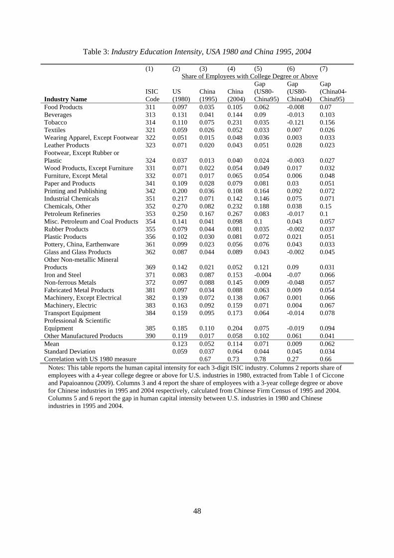
48

Table 3: Industry Education Intensity, USA 1980 and China 1995, 2004

(1) (2) (3) (4) (5) (6) (7)

Share of Employees with College Degree or Above

Industry Name ISIC Code

US (1980)

China (1995)

China (2004)

Gap (US80- China95)

Gap (US80- China04)

Gap (China04- China95)

Food Products 311 0.097 0.035 0.105 0.062 -0.008 0.07 Beverages 313 0.131 0.041 0.144 0.09 -0.013 0.103 Tobacco 314 0.110 0.075 0.231 0.035 -0.121 0.156 Textiles 321 0.059 0.026 0.052 0.033 0.007 0.026 Wearing Apparel, Except Footwear 322 0.051 0.015 0.048 0.036 0.003 0.033 Leather Products 323 0.071 0.020 0.043 0.051 0.028 0.023 Footwear, Except Rubber or Plastic 324 0.037 0.013 0.040 0.024 -0.003 0.027 Wood Products, Except Furniture 331 0.071 0.022 0.054 0.049 0.017 0.032 Furniture, Except Metal 332 0.071 0.017 0.065 0.054 0.006 0.048 Paper and Products 341 0.109 0.028 0.079 0.081 0.03 0.051 Printing and Publishing 342 0.200 0.036 0.108 0.164 0.092 0.072 Industrial Chemicals 351 0.217 0.071 0.142 0.146 0.075 0.071 Chemicals, Other 352 0.270 0.082 0.232 0.188 0.038 0.15 Petroleum Refineries 353 0.250 0.167 0.267 0.083 -0.017 0.1 Misc. Petroleum and Coal Products 354 0.141 0.041 0.098 0.1 0.043 0.057 Rubber Products 355 0.079 0.044 0.081 0.035 -0.002 0.037 Plastic Products 356 0.102 0.030 0.081 0.072 0.021 0.051 Pottery, China, Earthenware 361 0.099 0.023 0.056 0.076 0.043 0.033 Glass and Glass Products 362 0.087 0.044 0.089 0.043 -0.002 0.045 Other Non-metallic Mineral Products 369 0.142 0.021 0.052 0.121 0.09 0.031 Iron and Steel 371 0.083 0.087 0.153 -0.004 -0.07 0.066 Non-ferrous Metals 372 0.097 0.088 0.145 0.009 -0.048 0.057 Fabricated Metal Products 381 0.097 0.034 0.088 0.063 0.009 0.054 Machinery, Except Electrical 382 0.139 0.072 0.138 0.067 0.001 0.066 Machinery, Electric 383 0.163 0.092 0.159 0.071 0.004 0.067 Transport Equipment 384 0.159 0.095 0.173 0.064 -0.014 0.078 Professional & Scientific Equipment 385 0.185 0.110 0.204 0.075 -0.019 0.094 Other Manufactured Products 390 0.119 0.017 0.058 0.102 0.061 0.041 Mean

0.123 0.052 0.114 0.071 0.009 0.062

Standard Deviation

0.059 0.037 0.064 0.044 0.045 0.034 Correlation with US 1980 measure

0.67 0.73 0.78 0.27 0.66

Notes: This table reports the human capital intensity for each 3-digit ISIC industry. Columns 2 reports share of employees with a 4-year college degree or above for U.S. industries in 1980, extracted from Table 1 of Ciccone and Papaioannou (2009). Columns 3 and 4 report the share of employees with a 3-year college degree or above for Chinese industries in 1995 and 2004 respectively, calculated from Chinese Firm Census of 1995 and 2004. Columns 5 and 6 report the gap in human capital intensity between U.S. industries in 1980 and Chinese industries in 1995 and 2004.

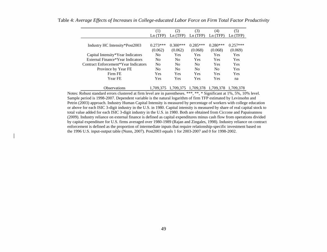
49

Table 4: Average Effects of Increases in College-educated Labor Force on Firm Total Factor Productivity

(1) (2) (3) (4) (5) Ln (TFP) Ln (TFP) Ln (TFP) Ln (TFP) Ln (TFP)

Industry HC Intensity*Post2003 0.273*** 0.300*** 0.285*** 0.280*** 0.257*** (0.062) (0.062) (0.068) (0.068) (0.069)

Capital Intensity*Year Indicators No Yes Yes Yes Yes External Finance*Year Indicators No No Yes Yes Yes

Contract Enforcement*Year Indicators No No No Yes Yes Province by Year FE No No No No Yes

Firm FE Yes Yes Yes Yes Yes Year FE Yes Yes Yes Yes na

Observations 1,709,375 1,709,375 1,709,378 1,709,378 1,709,378

Notes: Robust standard errors clustered at firm level are in parentheses. ***, **, * Significant at 1%, 5%, 10% level. Sample period is 1998-2007. Dependent variable is the natural logarithm of firm TFP estimated by Levinsohn and Petrin (2003) approach. Industry Human Capital Intensity is measured by percentage of workers with college education or above for each ISIC 3-digit industry in the U.S. in 1980. Capital intensity is measured by share of real capital stock to total value added for each ISIC 3-digit industry in the U.S. in 1980. Both are obtained from Ciccone and Papaioannou (2009). Industry reliance on external finance is defined as capital expenditures minus cash flow from operations divided by capital expenditure for U.S. firms averaged over 1980-1989 (Rajan and Zingales, 1998). Industry reliance on contract enforcement is defined as the proportion of intermediate inputs that require relationship-specific investment based on the 1996 U.S. input-output table (Nunn, 2007). Post2003 equals 1 for 2003-2007 and 0 for 1998-2002.

50

Table 5: Dynamic Effects of Increases in College-Educated Labor Force on Firm TFP

(1) (2) (3) (4) (5) (6) (7) Placebo Tests Baseline Controlling

Industry Trend Controlling Past Period Ln (TFP)

Controlling Pre-trends (Hornbeck,

2012)

US 1987 SIC 4-digit industry

Taiwan Japan

Industry HC Intensity*1999 0.099 0.199 0.122 -0.000 -0.273* 0.151 (0.121) (0.142) (0.122) (0.063) (0.143) (0.095)

Industry HC Intensity*2000 -0.100 0.010 -0.079 0.000 -0.379** 0.016 (0.121) (0.151) (0.122) (0.061) (0.163) (0.192)

Industry HC Intensity*2001 0.007 0.131 0.035 -0.000 -0.309* 0.301 (0.113) (0.153) (0.114) (0.057) (0.179) (0.250)

Industry HC Intensity*2002 0.173 0.308* 0.208* -0.000 -0.214 -0.626 0.402 (0.119) (0.162) (0.121) (0.054) (0.223) (0.805) (0.281)

Industry HC Intensity*2003 0.354*** 0.506*** 0.390*** 0.543*** -0.199 -1.035 0.389 (0.108) (0.159) (0.111) (0.051) (0.236) (0.893) (0.304)

Industry HC Intensity*2004 0.359*** 0.518*** 0.374*** 0.600*** 0.052 -1.351 0.400 (0.113) (0.164) (0.116) (0.042) (0.251) (0.869) (0.410)

Industry HC Intensity*2005 0.310*** 0.469*** 0.310*** 0.555*** -0.050 0.289 (0.112) (0.163) (0.115) (0.042) (0.289) (0.476)

Industry HC Intensity*2006 0.175 0.332** 0.197* 0.489*** -0.083 -0.206 (0.110) (0.162) (0.113) (0.040) (0.324) (0.511)

Industry HC Intensity*2007 0.267** 0.423*** 0.293*** 0.677*** 0.527 -0.280 (0.110) (0.162) (0.113) (0.037) (0.366) (0.589)

Capital Intensity*Year Indicators Yes Yes Yes Yes Yes Yes Yes External Finance*Year Indicators Yes Yes Yes Yes Yes Yes Yes

Contract Enforcement*Year Indicators Yes Yes Yes Yes Yes Yes Yes Province by Year FE Yes Yes Yes Yes N.A. N.A. N.A. Linear Industry Trend No Yes No No No No No

1995 Industry ln(TFP)*Year Indicators No No Yes No No No No 1998-2002 ln(TFP)*Year Indicators No No No Yes No No No

Firm/Industry FE Yes Yes Yes Yes Yes Yes Yes Year FE Yes Yes Yes

Observations 1,709,375 1,709,375 1,654,684 1,709,375 4,510 4,944 550 Notes: Robust standard errors clustered at firm level (columns 1-4 and 6) and industry level (columns 5 and 7) are in parentheses. ***, **, * Significant at 1%, 5%, 10% level. Columns 1-4 use Chinese firm data; sample period is 1998-2007, and dependent variable is the natural logarithm of firm TFP estimated by Levinsohn and Petrin (2003) approach. Column 5 uses U.S. industry data obtained from the NBER-CES Manufacturing Industry Database; sample period is 1998-2007, and dependent variable is the natural logarithm of TFP in each 1987 SIC 4-digit industry. Column 6 uses Taiwan firm-year level data; sample period is 2000, 2002-2004. Column 7 uses industry data obtained from Japan Industrial Productivity (JIP) database; sample period is 1998-2007. Industry Human Capital Intensity is measured by percentage of workers with college education or above for each ISIC 3-digit industry in the U.S. in 1980. Measures of capital intensity, industry reliance on external finance, and industry reliance on contract enforcement are the same as in Table 4.

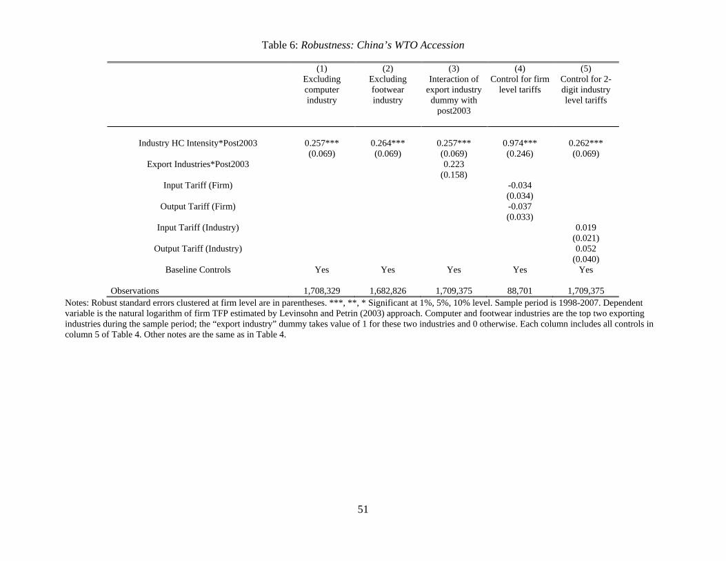
51

Table 6: Robustness: China’s WTO Accession

(1) (2) (3) (4) (5) Excluding

computer industry

Excluding footwear industry

Interaction of export industry

dummy with post2003

Control for firm level tariffs

Control for 2-digit industry level tariffs

Industry HC Intensity*Post2003 0.257*** 0.264*** 0.257*** 0.974*** 0.262*** (0.069) (0.069) (0.069) (0.246) (0.069)

Export Industries*Post2003 0.223 (0.158)

Input Tariff (Firm) -0.034 (0.034)

Output Tariff (Firm) -0.037 (0.033)

Input Tariff (Industry) 0.019 (0.021)

Output Tariff (Industry) 0.052 (0.040)

Baseline Controls Yes Yes Yes Yes Yes Observations 1,708,329 1,682,826 1,709,375 88,701 1,709,375

Notes: Robust standard errors clustered at firm level are in parentheses. ***, **, * Significant at 1%, 5%, 10% level. Sample period is 1998-2007. Dependent variable is the natural logarithm of firm TFP estimated by Levinsohn and Petrin (2003) approach. Computer and footwear industries are the top two exporting industries during the sample period; the “export industry” dummy takes value of 1 for these two industries and 0 otherwise. Each column includes all controls in column 5 of Table 4. Other notes are the same as in Table 4.

52

Table 7: Robustness: Using Regional Variation in College Graduates to Deal with WTO Accession and Other Macroeconomic Shocks

(1) (2) (3) (4) (5) (6) (7) Shock is defined as the increase in new college

graduates between 2001 and 2003 relative to 2001 labor force

Shock is defined as the increase in new college graduates between 2000-

2001 and 2003-2004 relative to the labor force in 2000-2001

Province-year share of new college grads in the labor force

Above median

Below median

Top tercile

Bottom 2 terciles

Above median Below median

Industry HC Intensity*Post2003 0.308*** 0.054 0.356*** 0.185** 0.300*** 0.012 0.215*** (0.078) (0.145) (0.113) (0.087) (0.074) (0.182) (0.069) Industry HC Intensity*Post2003* Province-year share of new college grads

0.689*** (0.265)

Baseline Controls Yes Yes Yes Yes Yes Yes Yes Observations 1,272,469 436,906 627,952 1,081,423 1,419,280 290,095 1,709,375

Notes: Robust standard errors clustered at firm level are in parentheses. ***, **, * Significant at 1%, 5%, 10% level. Sample period is 1998-2007. Dependent variable is the natural logarithm of firm TFP estimated by Levinsohn and Petrin (2003) approach. Industry Human Capital Intensity is measured by percentage of workers with college education or above for each ISIC 3-digit industry in the U.S. in 1980. In columns 1-4, college graduate shock is defined as the increase in new college graduates between 2001 and 2003 relative to 2001 labor force; in columns 5-6, it is defined as the increase in new college graduates between 2000-2001 and 2003-2004 relative to the labor force in 2000-2001. In column 7, we add a triple interaction term between Industry HC Intensity*Post2003 and province-year share of new college graduates in the labor force. Each column includes all controls in column 5 of Table 4. Other notes are the same as in Table 4.

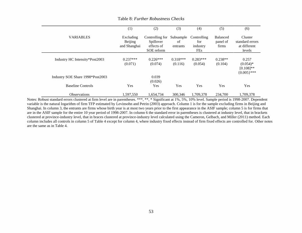
53

Table 8: Further Robustness Checks

(1) (2) (3) (4) (5) (6)

VARIABLES Excluding Beijing

and Shanghai

Controlling for Spillover effects of

SOE reform

Subsample of

entrants

Controlling for

industry FEs

Balanced panel of

firms

Cluster standard errors

at different levels

Industry HC Intensity*Post2003 0.237*** 0.226*** 0.318*** 0.283*** 0.238** 0.257

(0.071) (0.074) (0.116) (0.054) (0.104) (0.054)* [0.108]** {0.005}***

Industry SOE Share 1998*Post2003 0.039 (0.026)

Baseline Controls Yes Yes Yes Yes Yes Yes

Observations 1,597,550 1,654,734 300,346 1,709,378 234,700 1,709,378 Notes: Robust standard errors clustered at firm level are in parentheses. ***, **, * Significant at 1%, 5%, 10% level. Sample period is 1998-2007. Dependent variable is the natural logarithm of firm TFP estimated by Levinsohn and Petrin (2003) approach. Column 1 is for the sample excluding firms in Beijing and Shanghai. In column 3, the entrants are firms whose birth year is at most two years prior to the first appearance in the ASIF sample; column 5 is for firms that are in the ASIF sample for the entire 10 year period of 1998-2007. In column 6 the standard error in parentheses is clustered at industry level, that in brackets clustered at province-industry level, that in braces clustered at province-industry level calculated using the Cameron, Gelbach, and Miller (2011) method. Each column includes all controls in column 5 of Table 4 except for column 4, where industry fixed effects instead of firm fixed effects are controlled for. Other notes are the same as in Table 4.

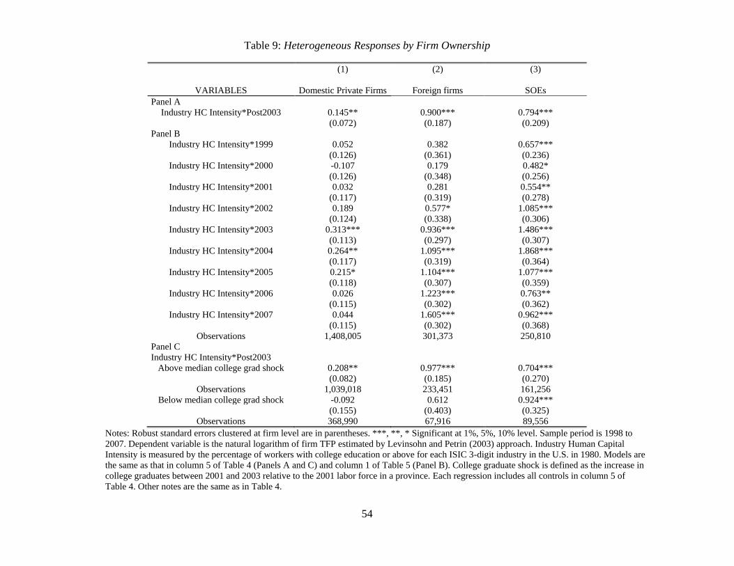
54

Table 9: Heterogeneous Responses by Firm Ownership

(1) (2) (3)

VARIABLES Domestic Private Firms Foreign firms SOEs Panel A

Industry HC Intensity*Post2003 0.145** 0.900*** 0.794*** (0.072) (0.187) (0.209)

Panel B Industry HC Intensity*1999 0.052 0.382 0.657***

(0.126) (0.361) (0.236) Industry HC Intensity*2000 -0.107 0.179 0.482*

(0.126) (0.348) (0.256) Industry HC Intensity*2001 0.032 0.281 0.554**

(0.117) (0.319) (0.278) Industry HC Intensity*2002 0.189 0.577* 1.085***

(0.124) (0.338) (0.306) Industry HC Intensity*2003 0.313*** 0.936*** 1.486***

(0.113) (0.297) (0.307) Industry HC Intensity*2004 0.264** 1.095*** 1.868***

(0.117) (0.319) (0.364) Industry HC Intensity*2005 0.215* 1.104*** 1.077***

(0.118) (0.307) (0.359) Industry HC Intensity*2006 0.026 1.223*** 0.763**

(0.115) (0.302) (0.362) Industry HC Intensity*2007 0.044 1.605*** 0.962***

(0.115) (0.302) (0.368) Observations 1,408,005 301,373 250,810

Panel C Industry HC Intensity*Post2003

Above median college grad shock 0.208** 0.977*** 0.704*** (0.082) (0.185) (0.270)

Observations 1,039,018 233,451 161,256 Below median college grad shock -0.092 0.612 0.924***

(0.155) (0.403) (0.325) Observations 368,990 67,916 89,556

Notes: Robust standard errors clustered at firm level are in parentheses. ***, **, * Significant at 1%, 5%, 10% level. Sample period is 1998 to 2007. Dependent variable is the natural logarithm of firm TFP estimated by Levinsohn and Petrin (2003) approach. Industry Human Capital Intensity is measured by the percentage of workers with college education or above for each ISIC 3-digit industry in the U.S. in 1980. Models are the same as that in column 5 of Table 4 (Panels A and C) and column 1 of Table 5 (Panel B). College graduate shock is defined as the increase in college graduates between 2001 and 2003 relative to the 2001 labor force in a province. Each regression includes all controls in column 5 of Table 4. Other notes are the same as in Table 4.

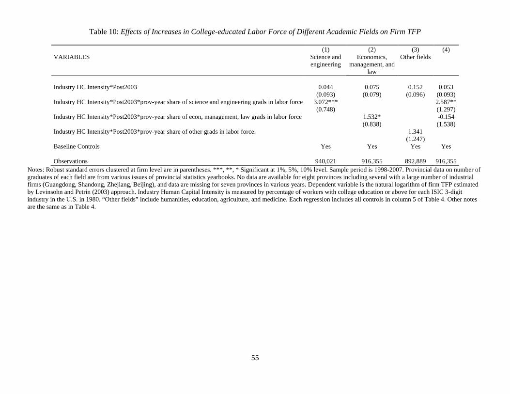
55

Table 10: Effects of Increases in College-educated Labor Force of Different Academic Fields on Firm TFP

(1) (2) (3) (4) VARIABLES Science and

engineering Economics,

management, and law

Other fields

Industry HC Intensity*Post2003 0.044 0.075 0.152 0.053 (0.093) (0.079) (0.096) (0.093) Industry HC Intensity*Post2003*prov-year share of science and engineering grads in labor force 3.072*** 2.587** (0.748) (1.297) Industry HC Intensity*Post2003*prov-year share of econ, management, law grads in labor force 1.532* -0.154 (0.838) (1.538) Industry HC Intensity*Post2003*prov-year share of other grads in labor force. 1.341 (1.247) Baseline Controls Yes Yes Yes Yes Observations 940,021 916,355 892,889 916,355

Notes: Robust standard errors clustered at firm level are in parentheses. ***, **, * Significant at 1%, 5%, 10% level. Sample period is 1998-2007. Provincial data on number of graduates of each field are from various issues of provincial statistics yearbooks. No data are available for eight provinces including several with a large number of industrial firms (Guangdong, Shandong, Zhejiang, Beijing), and data are missing for seven provinces in various years. Dependent variable is the natural logarithm of firm TFP estimated by Levinsohn and Petrin (2003) approach. Industry Human Capital Intensity is measured by percentage of workers with college education or above for each ISIC 3-digit industry in the U.S. in 1980. “Other fields” include humanities, education, agriculture, and medicine. Each regression includes all controls in column 5 of Table 4. Other notes are the same as in Table 4.

56

Table 11: Impact of Increases in College-Educated Labor Force on Firm's Technology Adoption (1) (2) (3) (4) (5) (6) (7) (8) Ln (TFP) Ln (1+ value of

imported high tech capital

goods)

Ln (average price of imported

high tech capital goods)

Number of different high tech

capital goods

Ln (capital stock per

worker)

Ln (1+Research Investment)

Ln (1+Training Investment)

Ln (1+Value of New

Products)

Panel A Industry HC Intensity*Post2003 0.872*** 2.949*** 1.493** 0.238 0.321*** 0.853*** 0.486*** 0.480*** (0.232) (0.725) (0.633) (0.749) (0.119) (0.153) (0.110) (0.152) Baseline Controls Yes Yes Yes Yes Yes Yes Yes Yes Panel B

Industry HC Intensity*1999 0.116 (0.182)

Industry HC Intensity*2000 -0.083 (0.189)

Industry HC Intensity*2001 0.011 -0.237 1.393 0.640 0.104 -0.078 (0.343) (1.073) (0.997) (0.906) (0.147) (0.197)

Industry HC Intensity*2002 0.112 1.519 1.021 0.372 0.309** 0.214 -0.062 0.145 (0.381) (1.091) (1.010) (0.945) (0.149) (0.132) (0.101) (0.197)

Industry HC Intensity*2003 0.786** 2.573** 1.663* 0.476 0.428*** 0.378* (0.342) (1.082) (0.979) (1.002) (0.159) (0.198)

Industry HC Intensity*2004 1.062*** 2.756** 1.922** 1.291 0.517*** (0.352) (1.075) (0.979) (1.077) (0.166)

Industry HC Intensity*2005 0.793** 4.772*** 3.053*** 0.277 0.440** 0.609*** 0.079 0.705*** (0.343) (1.095) (1.016) (1.078) (0.172) (0.171) (0.087) (0.230)

Industry HC Intensity*2006 1.059*** 4.053*** 2.432** 0.027 0.444** 1.058*** 0.244*** 0.589** (0.339) (1.119) (1.038) (1.135) (0.181) (0.176) (0.093) (0.238)

Industry HC Intensity*2007 1.263*** 0.371*** 0.419* (0.182) (0.099) (0.241)

Baseline Controls Yes Yes Yes Yes Yes Yes Yes Yes Observations 168,641 169,332 89,372 169,332 168,641 1,029,300 1,254,833 1,483,802

Notes: Robust standard errors clustered at firm level are in parentheses. ***, **, * Significant at 1%, 5%, 10% level. Sample for columns 1-5 is importing firms in the 2000-2006 Customs Data matched to the ASIF database. Column 2 includes only firms with positive import value of high-tech capital goods. Sample for columns 6-8 is from ASIF. Sample period for columns 6 and 7 is 2001, 2002, and 2005-2007, for column 8 is 1998-2003 and 2005-2007. Industry Human Capital Intensity is measured by percentage of workers with college education or above for each ISIC 3-digit industry in the U.S. in 1980. Each regression includes all controls in column 5 of Table 4. Other notes are the same as in Table 4.

57

Table 12: Change in Education and Occupation Composition between 1995 and 2004 and Wage Dynamics

(1) (2) (3) (4) (5) (6) Dep Var: Difference between 1995 and 2004 in industry

percentage of employees

with college degree

or above

with high school

education

with junior high school edu or below

who are technician

or engineers

Ln (Average Wage)

Industry HC Intensity 0.491*** 0.227*** -0.460*** 0.331*** (0.073) (0.063) (0.098) (0.054) Industry HC Intensity*Post2003 0.022 (0.026) Industry HC Intensity*1999 0.013 (0.040) Industry HC Intensity*2000 0.063 (0.041) Industry HC Intensity*2001 0.134*** (0.041) Industry HC Intensity*2002 0.211*** (0.040) Industry HC Intensity*2003 0.201*** (0.040) Industry HC Intensity*2004 0.140*** (0.038) Industry HC Intensity*2005 0.081** (0.039) Industry HC Intensity*2006 0.119*** (0.039) Industry HC Intensity*2007 0.043 (0.040) Observations 426 426 426 426 1,709,378 1,709,378 Notes: Robust standard errors clustered at industry level are in parentheses. ***, **, * Significant at 1%, 5%, 10% level. Data for columns 1-4 are 4-digit industry level data aggregated from the 1995 and 2004 Firm Censuses. Data for columns 5-6 are from the ASIF database, and the sample period is 1998-2007. Industry Human Capital Intensity is measured by percentage of workers with college education or above for each ISIC 3-digit industry in the U.S. in 1980. Columns 1-4 control for industry capital intensity, reliance on external finance, and reliance on contract enforcement. Regressions in columns 5-6 include all controls in column 5 of Table 4.

58

Figure 1: Annual Growth Rate of College Admission and Number of College Students Enrolled in Each Year

Notes: The top panel plots the annual growth rate of college admission, equal to the number of students admitted to 3- or 4-year regular colleges in current year divided by the number for the previous year minus 1, and the annual growth rate of GDP. The bottom panel depicts the total number of students (in millions) enrolled in regular colleges and universities, including both undergraduate and graduate students. Data are from various issues of China Statistics Yearbook.

0.1

.2.3

.4

1995 2000 2005 2010year

annual growth rate of college admission

annual growth rate of GDP

510

1520

25

1995 2000 2005 2010year

college enrolment, in million

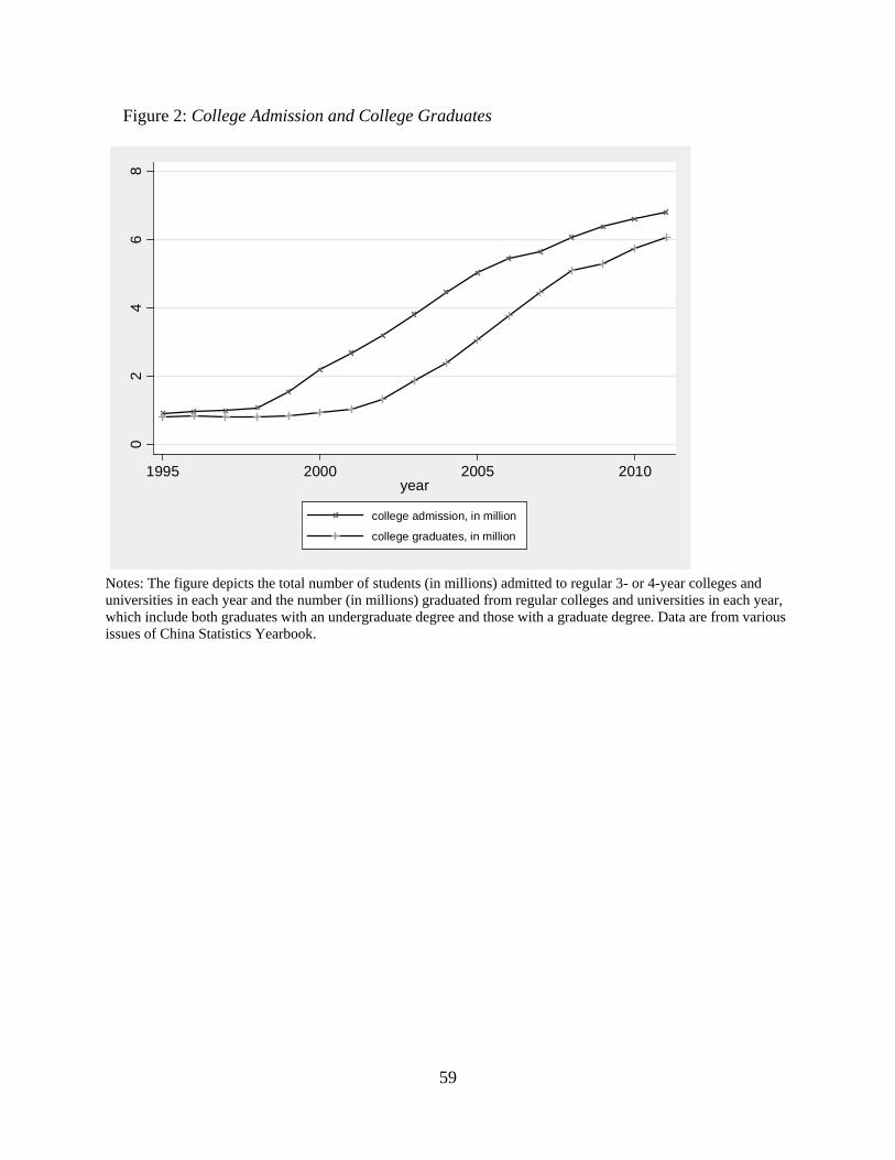
59

Figure 2: College Admission and College Graduates

Notes: The figure depicts the total number of students (in millions) admitted to regular 3- or 4-year colleges and universities in each year and the number (in millions) graduated from regular colleges and universities in each year, which include both graduates with an undergraduate degree and those with a graduate degree. Data are from various issues of China Statistics Yearbook.

02

46

8

1995 2000 2005 2010year

college admission, in million

college graduates, in million

60

Figure 3: Industry Human Capital Intensity and Productivity Growth post of Higher Education Expansion

Notes: Industries 1, 2, and 3 are the high, medium, and low human capital-intensity industries respectively. Height of each column is the firm performance in each industry if the frontier technology is employed. State A is the period before the higher education expansion, and it also indicates the highest level of firm performance in Industry 1 and Industry 2. State B is the period after the higher education expansion, and it also indicates the highest level of firm performance in Industry 1.

61

Figure 4: Firm Average ln(TFP) by Industry Human Capital Intensity

Notes: Each data point in the top panels is the average ln(TFP) of all firms in each year-industry cell, with 1998 values normalized to zero. Each data point in the bottom panel is the difference between the two lines in the top panel (Yt, above median – Yt, below median), with 1998 value normalized to zero. Firm TFP is estimated by the Levinsohn and Petrin (2003) approach.

0.2

.4.6

.81

1998 2000 2002 2004 2006 2008

Above Median HC Intensity Industries

Below Median HC Intensity Industries

A. Average TFP relative to 1998

0.0

2.0

4.0

6.0

8.1

1998 2000 2002 2004 2006 2008year

B. Average TFP relative to 1998, DD

62

Appendix A: Estimation of TFP

Our primary measure of firm performance is the Total Factor Productivity (TFP),

which is estimated using information on firm inputs and output. Consider the following

Cobb-Douglas production function:

0 1 2it it it ity l kβ β β η= + + + (A.1)

where ity is the natural logarithm of the value-added for firm i in year t , itl and itk are

the natural logarithm of labor and capital respectively. The residual term itη is firm

productivity. Let 1β and 2β denote estimates of 1β and 2β ; if we could estimate 1β

and 2β consistently, we can calculate firm TFP as follows:

1 2ˆˆ

it it it ittfp y l kβ β= − − (A.2)

Firm productivity is known to profit-maximizing firms but unobservable to

econometricians. Since a firm chooses its inputs based on its productivity shocks experienced

in the current period, the correlation between firm inputs and the residual term (i.e.,

productivity) could bias 1β and 2β . Thus the ordinary least square (OLS) estimation of

equation A.1 may lead to overestimation of 1β and 2β . Since profit-maximizing firms

respond to positive productivity shocks by increasing intermediate input usage and vice versa,

Levinsohn and Petrin (2003) suggest that one use intermediate inputs as a proxy for these

unobservable productivity shocks (i.e., LP method). In this paper, we employ the LP method

to estimate the firm level productivity.1 Another commonly used technique to estimate the

TFP is the method proposed by Olley and Pakes (1996, OP method), where the firm

investment is used as a proxy for unobserved firm productivity shocks.2

1 STATA command for LP method is levpet (Petrin et al., 2004).

Additionally,

Blundell and Bond (1998) suggest that in addition to controlling for firm and year fixed

effects, one can also use lags of labor and capital as instruments to consistently estimate the

2 STATA command for OP method is opreg (Yasar et al., 2008).

63

coefficients in Equation A.1, the system-GMM method.3

As robustness checks, we will use

TFPs estimated from the OLS, OP, and system-GMM methods as alternative measures.

LP Method

Suppose that the production technology is Cobb-Douglas as follows:

0it l it k it it itl kυ β β β ω η= + + + + (A.3)

where itυ denotes the natural logarithm of the value-added of firm i in year t , itl and

itk are the natural logarithm of labor and capital respectively. The transmitted productivity

component is denoted by itω , which is known to the firm but unobservable to

econometricians. Since itω not only affects firm inputs but also firm output directly, i.e., the

simultaneity problem in the production function estimation, estimators such as the OLS

ignoring this correlation between itω and inputs will yield inconsistent coefficient estimates

on labor and capital. itη is an error term assumed to be orthogonal to all the right-hand side

variables.

We assume that firm demand for intermediate input itm depends on firm i 's state

variables itk and itω , and ( , )it it it itm m k ω= . Relying on weak assumptions about firm

production technology, Levinsohn and Petrin (2003) show that the demand function of the

intermediate input is monotonically increasing with itω , and thus itω can be written as a

function of itk and itm , ( , )it it it itk mω ω= , allowing the use of the intermediate input as a

proxy for the unobserved firm productivity.

LP also assumes that firm productivity is governed by a first-order Markov process as

follows:

1( | )it it it itEω ω ω ξ−= + (A.4)

where itξ is an innovation to the productivity, which is uncorrelated with itk . Equation A.3

3 STATA command for system-GMM method is xtabond2 (Roodman 2009).

64

can thus be written as:

( , )it l it it it itl k mυ β φ η= + + (A.5)

where 0( , ) ( , )it it k it it it itk m k k mφ β β ω= + + . We approximate ( , )it itk mφ using a third-order

polynomial in itk and itm and estimate lβ consistently in the production function.

What remains is to obtain a consistent estimate of kβ . For any possible value of kβ∗ ,

we can predict itω as ˆˆit it k itkω φ β ∗= − . LP suggests a consistent approximation to

1( | )it itE ω ω − as follows:

2 31 0 1 1 2 1 3 1( | )it it it it it itE ω ω γ γ ω γ ω γ ω σ− − − −= + + + +

;

then a consistent estimate of kβ∗ can be obtained by minimizing the sample residual of the

production function using a golden section search algorithm

21

ˆ( ( | ))k

it it k it it itlt

min l k Eβ

υ β β ω ω∗

∗−− − −∑ (A.6)

OP Method

The OP method is based on the Olley and Pakes (1996) model of firm behavior.

Intuitively, incumbent firms decide whether to operate at the beginning of each period. If the

firm exits the market immediately, it receives a liquidation value of Φ . If the firm does not

exit, it chooses variable inputs (e.g., labor, capital, intermediate inputs) and an investment

level. Firm i 's decision problem is to maximise the expected discounted value of net future

profits. The Bellman equation can be written as

1 1 1 10

( , , ) max{ ,sup ( , , ) ( ) [ ( , , ) | ]}it

it it it it it it it it it it it it it iti

V a k a k c i E V a k Jω π ω ρ ω+ + + +≥

= Φ − + (A.7)

where ( )itπ ⋅ is the restricted profit function for firm i in period t , which is a function of

state variables, productivity itω , firm age ita , and firm capital itk . )( itc i is the cost of

investment iti in the current period and ρ is the discount factor. [ | ]itE J⋅ is the

expectation operator of firm i conditional on information itJ at time t . The implication of

65

the Bellman equation is that firm i will exit the market if its liquidation value Φ is larger

than its expected discounted returns; otherwise, firm i will stay in business and choose a

level of investment based on its productivity. The solution to this problem depends on the

Markov perfect Nash equilibrium which defines rules for exit and for investment decisions:

1 if 0 if otherwise

it itit

ω ωχ

≥=

(A.8)

( ), ,it it it iti i a kω= (A.9)

where itχ equals zero if firm i chooses to exit the market and equals one if firm f stays

in business and chooses an optimal investment level fti (constrained to be nonnegative).

Here, firm i 's sell-off value is lower than its expected discounted returns of staying in

business if and only if firm i 's productivity is larger than the cut-off value ( , )it it itk aω . The

investment equation implies that firm i 's decision depends on the productivity, age, and

capital stock, and firms experiencing a positive productivity shock in the current period will

invest more in the next period. Therefore, investment could act as a proxy for firm

productivity.

We augment the production function in Equation A.3 as follows:

0 l it k ii t a it it it tl k aυ β β β β ω η= + + + + + (A.10)

where ita is the age of the firm. Given standard assumptions of the model (e.g., random

sampling and linearity), the OLS generates biased and inconsistent estimates of coefficients

in equation A.10 for two reasons: the simultaneity problem due to the correlation between

itω and itl , itk and the selection bias resulting from the exit of unproductive firms. The

reason for the simultaneity problem is the same as that in the LP method. Regarding the

impact of selection bias, suppose that at the same level of productivity firms with a high

capital intensity is more profitable than firms with a low capital intensity, and this will cause

a negative correlation between the capital intensity and productivity in the next period since

66

low productivity firms with a low capital intensity will exit but low productivity firms with a

high capital intensity may survive. This potential correlation may cause a downward bias in

the estimate of kβ .

OP assumes that investment monotonically increases with productivity; therefore a

positive productivity shock in period t will cause firm i to invest more in that period for

any itk and ita . If we further assume that investment is strictly positive, itω could be

written as follows:

1( , , ) ( , , )it it it it it it iti i k a h i k aω −= = (A.11)

Substituting equation A.11 into equation A.10 yields

( , , )it l it it it it itl i k aυ β φ η= + + (A.12)

where 0( , , ) ( , , )it it it k it a it it it iti k a k a h i k aφ β β β= + + + . We can approximate ( , , )it it iti k aφ with

a second-order polynomial in age, labor, capital and a full set of their interactions. Since

investment is used as a proxy for productivity, OLS estimation of equation A.12 generates

consist estimate of lβ .

The exit rule in equation A.8 implies that the probability of survival for firm i in

period t depends on itω , itω and in turn on 1iti − , 1itk − , 1ita − . Following Yasar et al. (2008),

the predicted probability ˆ itp is calculated by regressing the probability of survival itχ on

1iti − , 1itk − , 1ita − and a full set of their interactions. In order to obtain consistent estimate of

kβ , we fit the following model using nonlinear least squares:

1 1 1 1ˆˆ ˆ( , )it l it k it a it it k it a it it it itl k a g k a pυ β β β φ β β ξ η− − − −− = + + − − + + (A.13)

where )(g ⋅ is proxied by a second-order polynomial in 1 1 1it k it a itk aφ β β− − −− + and 1ˆ itp − . We

then obtain consistent estimates of kβ and aβ , which, along with the consistent estimate of

lβ from the earlier step, allow us to estimate the firm level productivity.

In sum, the difference between the OP method and LP method is that OP uses

67

investment as a proxy for unobserved productivity shocks, whereas LP uses intermediate

inputs as a proxy for productivity shocks. The advantage of the LP over OP method is that

intermediate inputs may respond more smoothly to productivity shocks than investment. On

the other hand, the OP method has the advantage of allowing us to control for firm

self-selection in exiting the data set. Practically, in our main data investment is not directly

reported and has to be calculated from capital stock information for the same firm in two

consecutive years, which leads to missing observations that exit between the two years.

System-GMM Method

Under quite weak assumptions, the System-GMM method is a useful alternative

method to consistently estimate coefficients in production functions. Specifically, we add the

one-year lag of the firm value-added to Equation A.3:

1it l it k it v it it i t itl kυ β β β υ ω σ θ η−= + + + + + + (A.14)

where iσ is firm fixed effects controlling for all time invariant characteristics and tθ is

year fixed effects controlling for macroeconomic and policy shocks which are common to all

firms. Since itl , itk , and 1itυ − could be endogenous due to time varying omitted factors

included in itη , an instrumental variables strategy is used to estimate Equation A.14.

We take the first difference of equation (14) to eliminate firm level fixed effects iσ

1it l it k it v it it t itl kυ β β β υ ω θ η−∆ = ∆ + ∆ + ∆ + ∆ + ∆ + ∆ ; (A.15)

we then use all available lag levels as instruments for itl∆ , itk∆ , and 1itυ −∆ following the

difference-GMM method of Arellano and Bond (1991). The moment conditions are

( ) 0 for 2,..., and 1it s itE l t T sη− ∆ = =

( ) 0 for 2,..., and 1it s itE k t T sη− ∆ = =

( ) 0 for 3,..., and 2it s itE t T sυ η− ∆ = = .

In the System-GMM, we stack the level equations and first difference equations together and

68

use lag differences as instruments for the level equations. The additional moment conditions

for the level equations are:

[ ( )] 0 for 2,...,it i itE l t Tσ η∆ + = =

[ ( )] 0 for 2,...,it i itE k t Tσ η∆ + = =

1[ ( )] 0 for 3,...,it i itE t Tυ σ η−∆ + = =

Since there are more moment conditions than unknown parameters, consistent estimates of

lβ and kβ could be chosen by minimizing the distance of these moment conditions in the

system (Blundell and Bond, 1998).

Studies using this method to estimate the TFP include Blundell and Bond (2000),

Levinsohn and Petrin (2003), and Yu (2015). The disadvantage of the system-GMM method

is that it cannot control for time varying productivity shocks and the instruments used are

usually weak and their validity hard to test (Bun and Windmeijer 2010).

69

Appendix B: Aggregate TFP Growth

We calculate the contribution of new college graduates to the TFP growth of the

aggregate economy in the following two steps.

First, we consider the TFP growth of above-scale domestic-private and foreign-owned

firms in the manufacturing sector, the sample of our regression analyses. For firms in industry

j with human capital (HC) intensity jHC , on average, the extra TFP growth between

1998-2002 and 2003-2007 due to the surge in the college-educated labor force relative to the

least HC-intensive industry (with HC intensity 0HC ) is:

0( )j jz HC HCβ= ⋅ − , (B.1)

where β is the coefficient on the interaction between industry HC intensity and the

post-2003 dummy in Equation (1). We calculate the extra TFP growth for the entire sector as

the weighted sum of the extra TFP growth of each industry:

( )Ma j jj

s zz ⋅=∑ , (B.2)

where Ma stands for above-scale firms in the manufacturing sector, and the weight js is

the value-added share of industry j in this sector. Taking the estimate of β in column 5 of

Table 4 (0.257), jHC from column 2 of Table 3 with 0 0.037HC = for the footwear

industry, and the value-added share of industry j averaged over 2003-2007 for js , then

0.024MaZ = . Between 1998-2002 and 2003-2007 the overall TFP growth of the above-scale

manufacturing firms is 0.41; thus the extra TFP growth due to the HE expansion policy

accounts for 5.8% of the overall TFP growth, which is non-trivial given that the employment

of college-educated workers increases by just 6.2% in this sector.4

Second, we take into account of small firms and SOEs in the manufacturing sector

4 Education composition of employees by firm ownership and size is not available for this period, so we use the increase in the share of employees with a college education of the same type of firms between 1995 and 2004 as a proxy (column 7 of Table 3).

70

and firms in the service sector.5 β Assume that the interpretation of also applies to these

sectors, then the extra TFP growth of these sectors between 1998-2002 and 2003-2007 due to

the higher education (HE) expansion policy relative to the least HC-intensive manufacturing

industry can also be calculated as

0( )k kHCZ HCβ= ⋅ − , (B.3)

where ,k Mo Ser= for other firms in the manufacturing sector and for the service sector.

We then calculate the extra TFP growth for the entire economy as the weighted sum of the

extra TFP growth of each sector:

( )k kk

SZ Z⋅= ∑ , (B.4)

where , ,k Ma Mo Ser= for the three sectors, and kS is the value-added share of each sector

in the economy.6MoHC We proxy the value of by the average HC intensity of the US

manufacturing firms in 1980 (0.123, column 2 of Table 3), compute the value of SerHC (0.13)

based on data in Conti and Sulis (2016), and use the value-added share of each sector

averaged over 2003-2007 for kS (0.18, 0.22, and 0.48 respectively); the resulting value is

0.021Z = . Since the annual TFP growth of the Chinese economy for 1998-2007 is roughly

0.045 (Zhu, 2012), the extra TFP growth due to the HE expansion policy accounts for about 9%

of the TFP growth of the aggregate economy,7

The above calculations are based on the assumption that new college graduates

contribute similarly to the TFP growth in different types of firms and in different economic

a non-trivial amount given that the new

college-educated workers only accounted for 3.7% of total non-agricultural employees.

5 The service sector here is service sector plus construction, public utility, and quarry industries. Between 2002 and 2007, employees with at least a 4-year college education increased by 6.34 million in the service sector and 0.68 million in the manufacturing sector. We ignore the agriculture sector because only 0.2% agricultural employees have at least a 4-year college education in 2007. Data are from various issues of China Labor Statistics Yearbook. 6 For each above-scale manufacturing industry j, the value-added share in the entire economy is j j MasS S= ⋅ ;

thus ( ) ( )Ma Ma Ma j j j jZ S s z zS S⋅ = ⋅ ⋅ = ⋅∑ ∑ . 7 This is calculated as (0.021/5)/0.045=0.09, since Z is the extra TFP growth between two 5-year periods.

71

sectors. If, instead, their contribution in each sector depends on that sector’s productivity

growth, their contribution to the aggregate TFP growth may be different from the one

calculated above. For example, it may be smaller due to the much slower productivity growth

in the service sector than the manufacturing sector (He et al., 2014) – 7.2% and 5.8%

respectively if we assume the contribution to the TFP growth of college-educated workers in

the service sector is 60% and one-third of that in the manufacturing sector.

72

Appendix C: Regional Redistribution of Chinese Universities: 1955-1957

China’s higher education system is shaped by the central government’s restructuring

policies carried out in two stages in the 1950s. In the first stage, from 1951 to 1954, higher

education institutions (HEIs) are nationalised and reorganised following the Soviet model;

this is briefly discussed in Section 2.1. In the second stage, from 1955 to 1957, HEIs are

relocated from the coastal to the inland areas. This serves two goals: to foster the growth of

new industrial bases in the central and western provinces and to reduce the adverse impact of

potential wars along the coast, with the former also part of the strategy to cope with the latter.

The following measures are taken: (1) relocating entire departments or HEIs from the coastal

to central and western provinces; (2) expanding existing HEIs and establishing new ones in

the central and western provinces; (3) limiting the expansion of existing HEIs and the

construction of new ones in the coastal provinces. At the conclusion of this relocation effort

in 1957, the number of the HEIs and enrolment are roughly even between the coastal and

inland regions (Hao et al., 2011). Shaanxi, Sichuan, Hubei, Gansu, and Jilin are among the

provinces that gain the most from the relocation, while Jiangsu, Shandong, Beijing and

Shanghai lose. Provinces with a large ethnic minority population such as Xinjiang, Inner

Mongolia, and Qinghai also benefit from the central support for building new HEIs.

This "westward relocation" of HEIs has a profound impact on the regional distribution

of China's HE sector. Appendix Figure A3 plots the percentage of college enrolment in

population in selected years against that in 1957 for all provinces except for Beijing,

Shanghai, and Tianjin.8

8 Province names and abbreviations are listed in columns 2 and 3 of Appendix Table A3. It also reports the college enrolment rate in 1957 and college graduate shock in 2003. Chongqing (ChQ) was the largest city in Sichuan Province in the 1950s, and many of the new HE institutions relocated to Sichuan were in Chongqing.

There is a remarkably strong positive relationship between the

enrolment rate in 1957 and later years, reflecting the continued central control over the HE

sector. The correlation is close to 0.9 up to 1998, right before the higher education expansion

is set in motion, and only reduces to 0.81 and 0.68 for 2003 and 2010, post of the 1999

73

expansion. In contrast, the 1957 college enrolment rate is only weakly correlated with per

capita GDP and decreasing over time; in particular, it is merely 0.22 in 1998.9 Appendix

Figures A4 plots the per capita GDP in selected years against the 1957 college enrolment rate

for the subsample of provinces excluding Beijing, Shanghai, and Tianjin.10

In a simple regression of the provincial shock of college graduates, defined in Section

5.2 as the difference between the number of new college graduates in 2003 and 2001 relative

to the size of the labor force in 2001, college enrolment rate in 1957 alone explains 42% of

the variation for all provinces and 68% once the few outliers are excluded; adding per capita

GDP in 1998 increases the explanatory power to 65% and 75% respectively. Thus, the

magnitude of the HE expansion in the late 1990s and early 2000s is largely determined by

historical factors, which are at most weakly related to provincial economic performance in

the late 1990s and are controlled for by province-year fixed effects in the regressions.

9 The correlation is 0.53, 0.45, 0.29, 0.19 and 0.18 for 1957, 1982, 1992, 2003, and 2010 respectively. 10 The three large autonomous cities, Beijing, Shanghai, and Tianjin, are apparent outliers. They are much more developed in both economic activities and higher education. Other provinces are catching up in more recent years, but more in the per capita GDP than in the HE enrolment.

74

References:

Arellano, M. and Bond, S. (1991). ‘Some tests of specification for panel data: monte carlo

evidence and an application to employment equations’, Review of Economic Studies,

vol. 58(2), pp. 277-297.

Blundell, R. and Bond, S. (1998). ‘Initial conditions and moment restrictions in dynamic

panel data models’, Journal of Econometrics, vol. 87(1), pp. 115-143.

Blundell, R. and Bond, S. (2000). ‘GMM estimation with persistent panel data: an application

to production functions’, Econometric Reviews, vol. 19(3), pp. 321-340.

Bun, M.J.G. and Windmeijer, F. (2010). ‘The weak instrument problem of the system GMM

estimator in dynamic panel data models’, Econometrics Journal, vol. 13, pp. 95-126.

Conti M. and Sulis G. (2016). ‘Human capital, employment protection and growth in Europe’,

Journal of Comparative Economics, vol. 44(2), pp. 213-230.

Hao, W., Long, Z. and Zhang, J. (2011). ‘History of higher education of people's republic of

China . Beijing: the New World Press (in Chinese).

He, D., Zhang, W., Han, G. and Wu, T. (2014). ‘Productivity growth of the nontradable

sectors in China’, Review of Development Economics, vol. 18(4), pp. 655-666.

Levinsohn, J. and Petrin, A. (2003). ‘Estimating production functions using inputs to control

for unobservables’, Review of Economic Studies, vol. 70, pp. 317-341.

Olley, S.G. and Pakes, A. (1996). ‘The dynamics of productivity in the telecommunications

equipment industry’, Econometrica, vol. 64(6), pp. 1263-1297.

Petrin, A., Poi, B.P. and Levinsohn, J. (2004). ‘Production function estimation in Stata using

inputs to control for unobservables’, Stata Journal, vol. 4(2), pp. 113-123.

Roodman, D. (2009). ‘How to do Xtabond2: an introduction to difference and system GMM

in Stata’, Stata Journal, vol. 9(1), pp. 86-136.

Yasar, M., Raciborski, R. and Poi, B. (2008). ‘Production function estimation in Stata using

the Olley and Pakes method’, Stata Journal, vol. 8(2), pp. 221-231.

75

Yu, M. (2015). ‘Processing trade, tariff reductions and firm productivity: evidence from

Chinese firms’, Economic Journal, vol. 125, pp. 943-988.

Zhu, X. (2012). ‘Understanding China’s growth: Past, present, and future’, Journal of

Economic Perspectives, vol. 26(4), pp. 103-124.

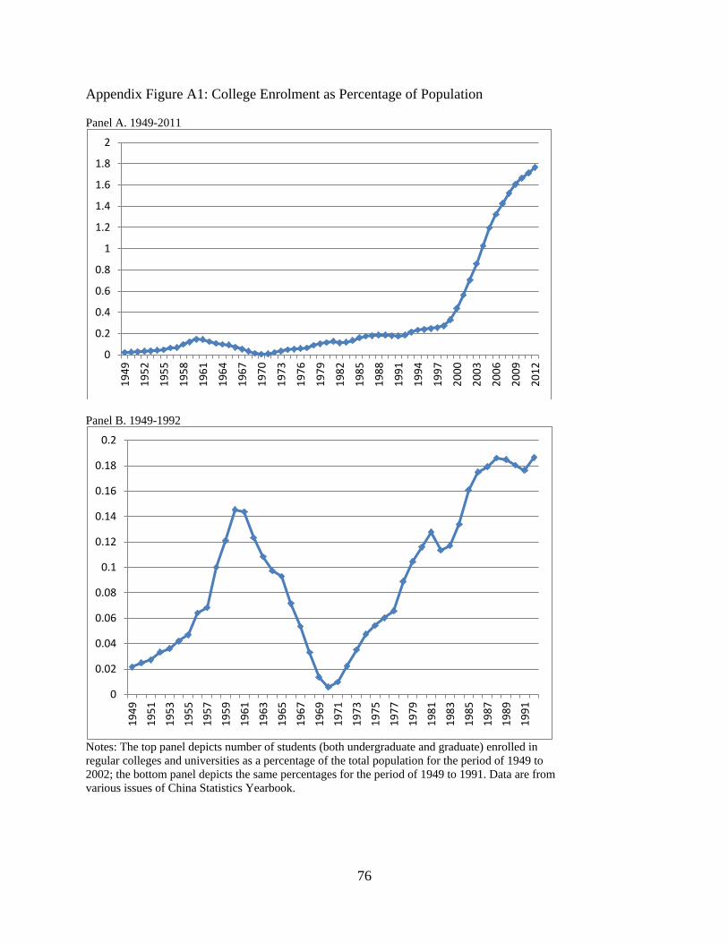
76

Appendix Figure A1: College Enrolment as Percentage of Population Panel A. 1949-2011

Panel B. 1949-1992

Notes: The top panel depicts number of students (both undergraduate and graduate) enrolled in regular colleges and universities as a percentage of the total population for the period of 1949 to 2002; the bottom panel depicts the same percentages for the period of 1949 to 1991. Data are from various issues of China Statistics Yearbook.

0

0.2

0.4

0.6

0.8

1

1.2

1.4

1.6

1.8

2 1

949

195

2

195

5

195

8

196

1

196

4

196

7

197

0

197

3

197

6

197

9

198

2

198

5

198

8

199

1

199

4

199

7

200

0

200

3

200

6

200

9

201

2

0

0.02

0.04

0.06

0.08

0.1

0.12

0.14

0.16

0.18

0.2

194

9 1

951

195

3 1

955

195

7 1

959

196

1 1

963

196

5 1

967

196

9 1

971

197

3 1

975

197

7 1

979

198

1 1

983

198

5 1

987

198

9 1

991

77

Appendix Figure A2: Annual Growth Rates of GDP and College Admission for Selected Provinces, 1995-2011

Notes: Each figure plots the annual growth rate of college admission, equal to the number of students admitted to 3- or 4-year regular colleges in current year divided by the number in the previous year minus 1 (solid dots), and the annual growth rate of GDP (solid diamonds). Beijing and Guangdong represent provinces on the coast, Hebei and Anhui those in central China, and Shaanxi and Sichuan those in the west. Data are from various issues of China Statistics Yearbook, China Education Statistics Yearbook, and provincial Statistics Yearbooks.

-.10

.1.2

.3

1995 2000 2005 2010year

Beijing

0.1

.2.3

.4.5

1995 2000 2005 2010year

Guangdong

0.1

.2.3

.4.5

1995 2000 2005 2010year

Hebei0

.2.4

.6

1995 2000 2005 2010year

Anhai

0.1

.2.3

.4.5

1995 2000 2005 2010year

Shaanxi

0.2

.4.6

1995 2000 2005 2010year

Sichuan

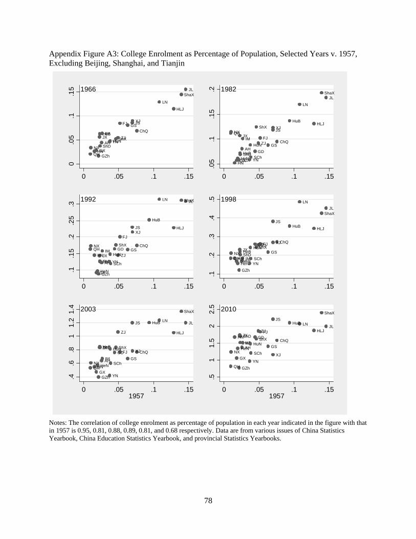
78

Appendix Figure A3: College Enrolment as Percentage of Population, Selected Years v. 1957, Excluding Beijing, Shanghai, and Tianjin

Notes: The correlation of college enrolment as percentage of population in each year indicated in the figure with that in 1957 is 0.95, 0.81, 0.88, 0.89, 0.81, and 0.68 respectively. Data are from various issues of China Statistics Yearbook, China Education Statistics Yearbook, and provincial Statistics Yearbooks.

HeBShX

IM

LN

JL

HLJ

JS

ZJAH

FJ

JX

ShDHuN

GXHN

ChQ

GZh

YN

ShaX

GS

QHNX

XJ

0.0

5.1

.15

0 .05 .1 .15

1966

HeB

ShX

IM

LNJL

HLJJS

ZJAH

FJJX

ShDHeN

HuB

HuNGD

GXHN

ChQ

SChGZh YN

ShaX

GS

QHNXXJ

.05

.1.1

5.2

0 .05 .1 .15

1982

HeB

ShXIM

LN JL

HLJJS

ZJ

AH

FJ

JXShD

HeN

HuB

HuNGD

GX

HN

ChQ

SCh

GZh

YN

ShaX

GSQHNX

XJ

.1.1

5.2

.25

.3

0 .05 .1 .15

1992

HeBShX

IM

LNJL

HLJ

JS

ZJ

AH

FJJXShD

HeN

HuB

HuNGD

GXHN

ChQ

SCh

GZhYN

ShaX

GSQHNX

XJ

.1.2

.3.4

.5

0 .05 .1 .15

1998

HeB ShX

IM

LN JL

HLJ

JS

ZJ

AH

FJJXShD

HeN

HuB

HuNGD

GXHN

ChQ

SCh

GZh YN

ShaX

GS

QHNX

XJ

.4.6

.81

1.2

1.4

0 .05 .1 .151957

2003

HeBShX

IM

LN JLHLJ

JS

ZJ

AH

FJJXShD

HeN

HuB

HuNGD

GX

HNChQ

SCh

GZhYN

ShaX

GS

QH

NXXJ

.51

1.5

22.

5

0 .05 .1 .151957

2010

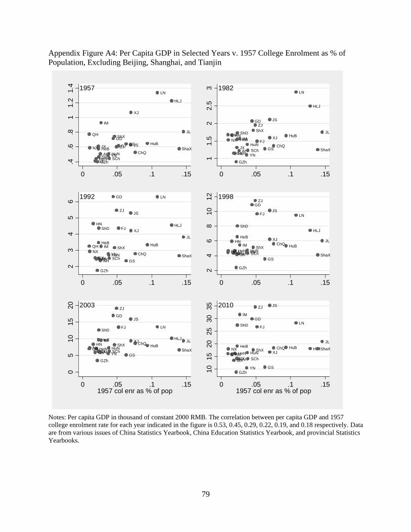
79

Appendix Figure A4: Per Capita GDP in Selected Years v. 1957 College Enrolment as % of Population, Excluding Beijing, Shanghai, and Tianjin

Notes: Per capita GDP in thousand of constant 2000 RMB. The correlation between per capita GDP and 1957 college enrolment rate for each year indicated in the figure is 0.53, 0.45, 0.29, 0.22, 0.19, and 0.18 respectively. Data are from various issues of China Statistics Yearbook, China Education Statistics Yearbook, and provincial Statistics Yearbooks.

HeB

ShX

IM

LN

JL

HLJ

JSZJ

AH

FJJX

ShDHeN

HuB

HuN

GD

GX

ChQSCh

GZhYN

ShaXGS

QH

NX

XJ

.4.6

.81

1.2

1.4

0 .05 .1 .15

1957

HeB

ShX

IM

LN

JL

HLJ

JSZJ

AH

FJJX

ShD

HeN

HuB

HuN

GD

GX

HN

ChQSCh

GZh

YNShaXGS

QHNX XJ

11.

52

2.5

3

0 .05 .1 .15

1982

HeBShXIM

LN

JL

HLJ

JSZJ

AH

FJ

JX

ShD

HeN

HuB

HuN

GD

GX

HN

ChQSCh

GZh

YN ShaXGS

QHNX

XJ

23

45

6

0 .05 .1 .15

1992

HeB

ShXIM

LN

JL

HLJ

JS

ZJ

AH

FJ

JX

ShD

HeNHuB

HuN

GD

GX

HN ChQ

SCh

GZh

YN ShaXGS

QHNX

XJ

24

68

1012

0 .05 .1 .15

1998

HeBShX

IM

LN

JLHLJ

JS

ZJ

AH

FJ

JX

ShD

HeNHuBHuN

GD

GX

HN ChQ

SCh

GZh

YNShaX

GSQHNX

XJ

05

1015

20

0 .05 .1 .151957 col enr as % of pop

2003

HeBShX

IM

LN

JL

HLJ

JSZJ

AH

FJ

JX

ShD

HeNHuB

HuN

GD

GXHN

ChQ

SCh

GZhYN

ShaX

GS

QHNX

XJ

1015

2025

3035

0 .05 .1 .151957 col enr as % of pop

2010

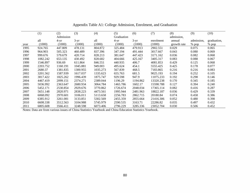
80

Appendix Table A1: College Admission, Enrolment, and Graduation

(1) (2) (3) (4) (5) (6) (7) (8) (9) (10)

year

all (1000)

Admission 4-yr (1000)

3-yr (1000)

all (1000)

Graduation 4-yr (1000)

3-yr (1000)

enrolment (1000)

admission, annual growth rate

admission, % pop

graduation, % pop

1995 924.765 447.809 478.131 804.872 325.484 479.913 2902.551 0.029 0.075 0.065 1996 964.903 505.323 460.489 837.396 347.194 491.444 3017.667 0.043 0.080 0.069 1997 999.676 579.679 420.714 828.213 381.647 447.423 3171.162 0.036 0.082 0.068 1998 1082.242 653.135 430.492 828.682 404.666 425.167 3405.317 0.083 0.088 0.067 1999 1546.897 936.69 611.864 846.551 440.935 406.7 4081.853 0.429 0.125 0.068 2000 2203.752 1160.191 1045.881 949.003 495.624 454.1 5555.425 0.425 0.178 0.077 2001 2680.37 1381.835 1300.955 1035.273 567.839 468.5 7183.865 0.216 0.216 0.083 2002 3201.562 1587.939 1617.037 1335.623 655.763 681.5 9025.193 0.194 0.252 0.105 2003 3817.422 1825.262 1996.439 1875.747 929.598 947.9 11075.233 0.192 0.298 0.146 2004 4467.419 2099.151 2374.271 2389.044 1196.29 1194.862 13320.238 0.170 0.345 0.185 2005 5036.992 2363.647 2680.934 3064.784 1465.786 1602.17 15598.788 0.127 0.394 0.240 2006 5452.171 2530.854 2929.676 3770.862 1726.674 2048.034 17365.114 0.082 0.416 0.287 2007 5651.148 2820.971 2838.223 4473.561 1995.944 2481.963 18822.187 0.036 0.429 0.339 2008 6068.092 2970.601 3106.011 5113.658 2256.783 2862.715 20180.84 0.074 0.458 0.386 2009 6385.912 3261.081 3133.851 5302.569 2455.359 2855.664 21416.306 0.052 0.480 0.398 2010 6608.338 3512.563 3104.988 5745.979 2590.535 3163.71 22286.82 0.035 0.497 0.432 2011 6805.608 3566.411 3248.598 6073.406 2796.229 3285.336 23052.704 0.030 0.506 0.452 Notes: Data are from various issues of China Statistics Yearbook and China Education Statistics Yearbook.

81

Appendix Table A2: Correlations between Alternative Measures of College Graduate Shock and Economic Growth Rate across Provinces

All provinces w/o Beijing, Tianjin, Shanghai Economic growth rate Shock 1 Shock 2 Shock 1 Shock 2 Per capita GDP growth rate 0.29 0.35

0.20 0.29

(0.11) (0.06)

(0.30) (0.13) Growth rate of number of manufacturing firms -0.04 -0.02

-0.03 0.01

(0.84) (0.92)

(0.89) (0.95) Growth rate of number of manufacturing firms in Industries with above median HC intensity -0.08 -0.06

-0.10 -0.06

(0.67) (0.74)

(0.60) (0.75) Growth rate of TFP of manufacturing firms 0.14 0.15

0.06 0.03

(0.44) (0.42)

(0.77) (0.87) Growth rate of TFP of manufacturing firms in Industries with above median HC intensity 0.21 0.17

0.24 0.18

(0.26) (0.35)

(0.21) (0.37) Growth rate of TFP of firms in the fabricated metal product industry (median HC intensity) -0.17 -0.17

-0.25 -0.24

(0.36) (0.37)

(0.19) (0.22) Growth rate of TFP of firms in the electric machinery industry (75th percentile of HC intensity) 0.12 0.09

0.30 0.25

(0.53) (0.63)

(0.12) (0.19) Notes: Authors’ calculation based on data from the Annual Survey of Industrial Firms, various issues of China Statistics Yearbook. Numbers in parentheses are p-values. All economic growth rates are annual growth rate from 1998 to 1999. College graduate Shock 1 is defined as the ratio between the growth of college graduates from 2001 to 2003 and the labor force in 2001; college graduate Shock 2 is defined as the difference between the average number of college graduates in 2003 and 2004 and that in 2000 and 2001 normalized by the average size of labor force in 2000 and 2001. All variables are at the provincial level.

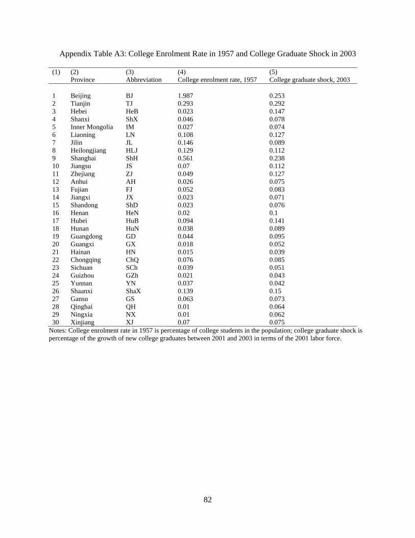
82

Appendix Table A3: College Enrolment Rate in 1957 and College Graduate Shock in 2003 (1) (2) (3) (4) (5)

Province Abbreviation College enrolment rate, 1957 College graduate shock, 2003

1 Beijing BJ 1.987 0.253 2 Tianjin TJ 0.293 0.292 3 Hebei HeB 0.023 0.147 4 Shanxi ShX 0.046 0.078 5 Inner Mongolia IM 0.027 0.074 6 Liaoning LN 0.108 0.127 7 Jilin JL 0.146 0.089 8 Heilongjiang HLJ 0.129 0.112 9 Shanghai ShH 0.561 0.238 10 Jiangsu JS 0.07 0.112 11 Zhejiang ZJ 0.049 0.127 12 Anhui AH 0.026 0.075 13 Fujian FJ 0.052 0.083 14 Jiangxi JX 0.023 0.071 15 Shandong ShD 0.023 0.076 16 Henan HeN 0.02 0.1 17 Hubei HuB 0.094 0.141 18 Hunan HuN 0.038 0.089 19 Guangdong GD 0.044 0.095 20 Guangxi GX 0.018 0.052 21 Hainan HN 0.015 0.039 22 Chongqing ChQ 0.076 0.085 23 Sichuan SCh 0.039 0.051 24 Guizhou GZh 0.021 0.043 25 Yunnan YN 0.037 0.042 26 Shaanxi ShaX 0.139 0.15 27 Gansu GS 0.063 0.073 28 Qinghai QH 0.01 0.064 29 Ningxia NX 0.01 0.062 30 Xinjiang XJ 0.07 0.075

Notes: College enrolment rate in 1957 is percentage of college students in the population; college graduate shock is percentage of the growth of new college graduates between 2001 and 2003 in terms of the 2001 labor force.

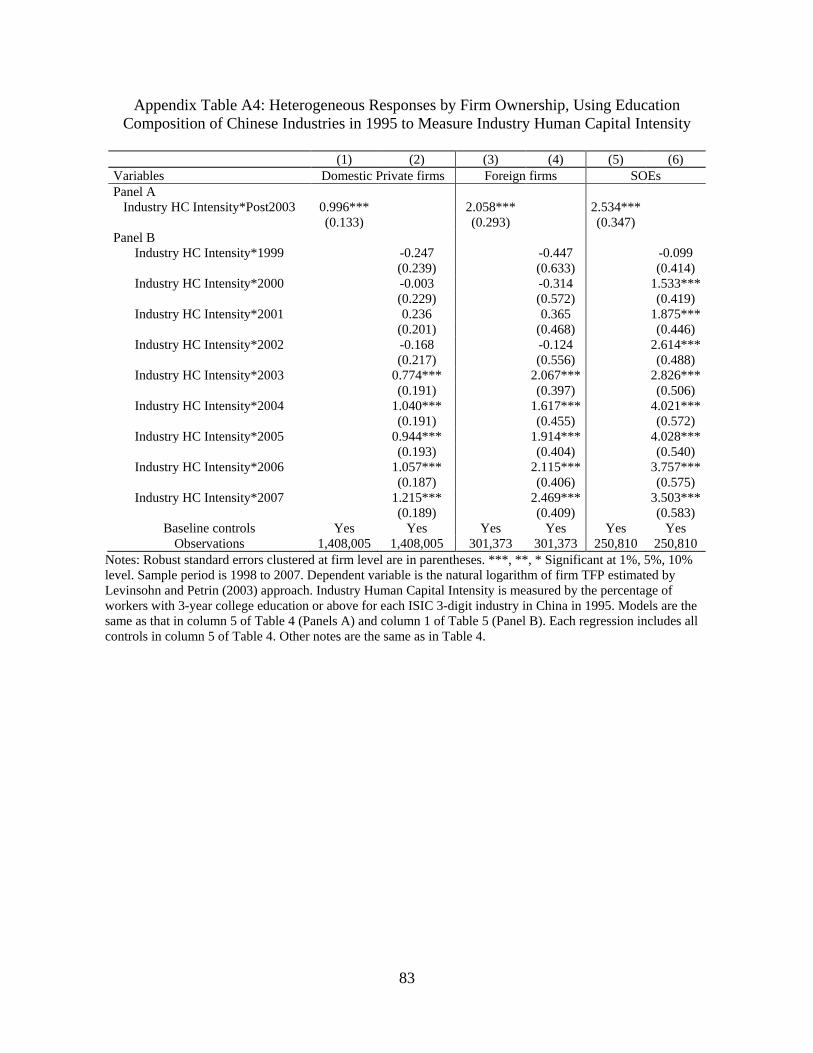
83

Appendix Table A4: Heterogeneous Responses by Firm Ownership, Using Education Composition of Chinese Industries in 1995 to Measure Industry Human Capital Intensity

(1) (2) (3) (4) (5) (6) Variables Domestic Private firms Foreign firms SOEs Panel A

Industry HC Intensity*Post2003 0.996*** 2.058*** 2.534*** (0.133) (0.293) (0.347) Panel B

Industry HC Intensity*1999 -0.247 -0.447 -0.099 (0.239) (0.633) (0.414)

Industry HC Intensity*2000 -0.003 -0.314 1.533*** (0.229) (0.572) (0.419)

Industry HC Intensity*2001 0.236 0.365 1.875*** (0.201) (0.468) (0.446)

Industry HC Intensity*2002 -0.168 -0.124 2.614*** (0.217) (0.556) (0.488)

Industry HC Intensity*2003 0.774*** 2.067*** 2.826*** (0.191) (0.397) (0.506)

Industry HC Intensity*2004 1.040*** 1.617*** 4.021*** (0.191) (0.455) (0.572)

Industry HC Intensity*2005 0.944*** 1.914*** 4.028*** (0.193) (0.404) (0.540)

Industry HC Intensity*2006 1.057*** 2.115*** 3.757*** (0.187) (0.406) (0.575)

Industry HC Intensity*2007 1.215*** 2.469*** 3.503*** (0.189) (0.409) (0.583)

Baseline controls Yes Yes Yes Yes Yes Yes Observations 1,408,005 1,408,005 301,373 301,373 250,810 250,810

Notes: Robust standard errors clustered at firm level are in parentheses. ***, **, * Significant at 1%, 5%, 10% level. Sample period is 1998 to 2007. Dependent variable is the natural logarithm of firm TFP estimated by Levinsohn and Petrin (2003) approach. Industry Human Capital Intensity is measured by the percentage of workers with 3-year college education or above for each ISIC 3-digit industry in China in 1995. Models are the same as that in column 5 of Table 4 (Panels A) and column 1 of Table 5 (Panel B). Each regression includes all controls in column 5 of Table 4. Other notes are the same as in Table 4.

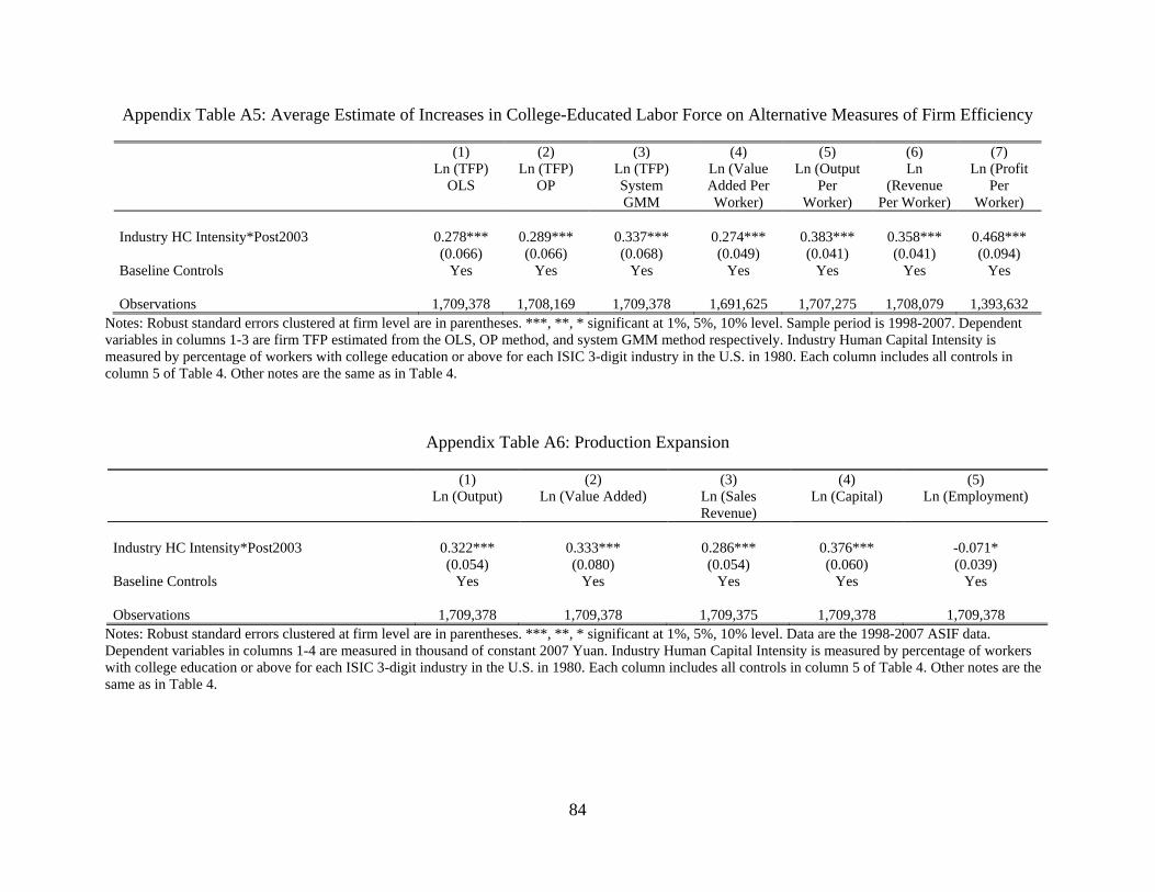
84

Appendix Table A5: Average Estimate of Increases in College-Educated Labor Force on Alternative Measures of Firm Efficiency

(1) (2) (3) (4) (5) (6) (7) Ln (TFP)

OLS Ln (TFP)

OP Ln (TFP) System GMM

Ln (Value Added Per Worker)

Ln (Output Per

Worker)

Ln (Revenue

Per Worker)

Ln (Profit Per

Worker) Industry HC Intensity*Post2003 0.278*** 0.289*** 0.337*** 0.274*** 0.383*** 0.358*** 0.468*** (0.066) (0.066) (0.068) (0.049) (0.041) (0.041) (0.094) Baseline Controls Yes Yes Yes Yes Yes Yes Yes Observations 1,709,378 1,708,169 1,709,378 1,691,625 1,707,275 1,708,079 1,393,632

Notes: Robust standard errors clustered at firm level are in parentheses. ***, **, * significant at 1%, 5%, 10% level. Sample period is 1998-2007. Dependent variables in columns 1-3 are firm TFP estimated from the OLS, OP method, and system GMM method respectively. Industry Human Capital Intensity is measured by percentage of workers with college education or above for each ISIC 3-digit industry in the U.S. in 1980. Each column includes all controls in column 5 of Table 4. Other notes are the same as in Table 4.

Appendix Table A6: Production Expansion

(1) (2) (3) (4) (5) Ln (Output) Ln (Value Added) Ln (Sales

Revenue) Ln (Capital) Ln (Employment)

Industry HC Intensity*Post2003 0.322*** 0.333*** 0.286*** 0.376*** -0.071* (0.054) (0.080) (0.054) (0.060) (0.039) Baseline Controls Yes Yes Yes Yes Yes Observations 1,709,378 1,709,378 1,709,375 1,709,378 1,709,378

Notes: Robust standard errors clustered at firm level are in parentheses. ***, **, * significant at 1%, 5%, 10% level. Data are the 1998-2007 ASIF data. Dependent variables in columns 1-4 are measured in thousand of constant 2007 Yuan. Industry Human Capital Intensity is measured by percentage of workers with college education or above for each ISIC 3-digit industry in the U.S. in 1980. Each column includes all controls in column 5 of Table 4. Other notes are the same as in Table 4.