Human Capital Theory and the Life-Cycle Pattern of ...paulgomme.github.io/lifecycle.pdf · Human Capital Theory and the Life-Cycle Pattern of Learning and Earning, Income and Wealth

Human Capital Theory and the Life-Cycle Pattern ofLearning and Earning, Income and Wealth

David AndolfattoSimon Fraser University

Christopher FerrallQueen’s University

Paul GommeFederal Reserve Bank of Cleveland

May 2000

Abstract

Life-cycle patterns of income, earnings, consumption, labor supply, and wealth vary sys-tematically across educational groups. Human capital theory explains different educationalchoices in terms of parameters describing tastes and technology. We ask whether differencesin these parameters are also consistent with other patterns of behavior. Our preliminary find-ings suggest that no single form of parameter heterogeneity will be able to account for the jointbehavior of life-cycle choices.

1 Introduction

Individuals with different educational backgrounds differ significantly and systematically in their

economic behavior over the life-cycle. It is well-known, for example, that well-educated individ-

uals tend to have higher income and earnings throughout most of the life-cycle. Most of their

higher earnings are in the form of higher wages, but they also tend to work more. In addition, they

tend to consume more and accumulate financial wealth at a faster rate. What accounts for these

differences?

Unlike demographic variables such as age, sex, and race, educational attainment (or human

capital accumulation in general) is largely a choice variable. From an early age, individuals are

taught about the benefits of schooling. Teenagers are warned about the consequences of failing

to complete their high-school education and they are generally made aware of the high returns

associated with a college degree. Yet, individuals quite clearly make different choices concerning

educational attainment; to a first approximation, roughly 25% of the population does not complete

high-school, 50% complete high-school, and 25% attain a college degree. Casual empiricism

suggests that lifetime learning expenditures and learning efforts devoted to more general human

capital accumulation activities are highly correlated with the schooling decision. What determines

these choices?

One way to understand the human capital choice is in terms of an optimal investment decision;

see Ben-Porath (1967). In the Ben-Porath model, individuals seek to maximize the present value

of their lifetime earnings by allocating their time between work and learning activities, and by

choosing an appropriate expenditure path for educational goods and services. A key parameter in

this model is the ‘ability to learn’, modeled as the technological efficiency with which learning

effort and resources augment the value of human capital.1 Not surprisingly, the model predicts that

more able individuals choose to undertake greater human capital investments, especially early on

in the life-cycle, and that learning effort declines over time. During youth, less able individuals

1Another way to model learning ability is in terms of initial endowments of human capital.

1

tend to earn more (as they devote more time to work rather than learning), but more able individuals

have rapidly rising earning profiles that soon overtake those of the less able. In addition, dispersion

in earnings across educational groups tends to grow over time. These predictions are broadly

consistent with the evidence; e.g., see Lillard (1977).

We think that the basic Ben-Porath model featuring differences in learning ability provides

a plausible interpretation of why educational attainment differs across individuals as well as ex-

plaining how these different human capital accumulation patterns translate into different earnings

profiles. However, before one can be confident that ability differences are at the root of inequality,

it would be prudent to examine whether the human capital model is consistent with the observed

lifetime profiles of other important economic variables, such as consumption, leisure (labor), and

financial asset accumulation (capital income). In order to address this question, we augment the

basic human capital model along the lines of Blinder and Weiss (1976), Heckman (1976), and Ry-

der, Stafford, and Stephan (1976), who explicitly model the labor-leisure choice. Judging by what

is reported in the recent survey by Neal and Rosen (2000), these versions of the human capital

model represent the extent to which theory has currently been developed.

Blinder and Weiss (1976) are primarily concerned with determining the conditions under which

the age profiles of human capital, wages, leisure, and learning behave in a ‘normal’ manner; see

their Figure 5. Their main finding is that ‘normal’ behavior arises when the rate of time prefer-

ence is sufficiently ‘small’.2 They do not ask how other parameters (in particular, learning ability)

affect life-cycle behavior, nor do they comment on consumption and asset accumulation. Ryder

et al.(1976) also demonstrate that many qualitatively different life-cycle patterns are possible and,

in particular, there are cases in which small differences in initial endowments can result in dra-

matically different behavior. Heckman (1976) reports the results of several comparative dynamics

exercises, but does not always provide a full description of behavior. For example, he finds that

individuals with greater learning ability have peaks in their hours of work profiles at older ages,

2To the extent that schooling entails foregone leisure, very impatient individuals may prefer to postpone theirschooling and work effort to later stages of the life-cycle.

2

but we are not told whether these profiles are generally higher or lower. Similarly, he does not ask

how differences in ability affect financial asset accumulation.

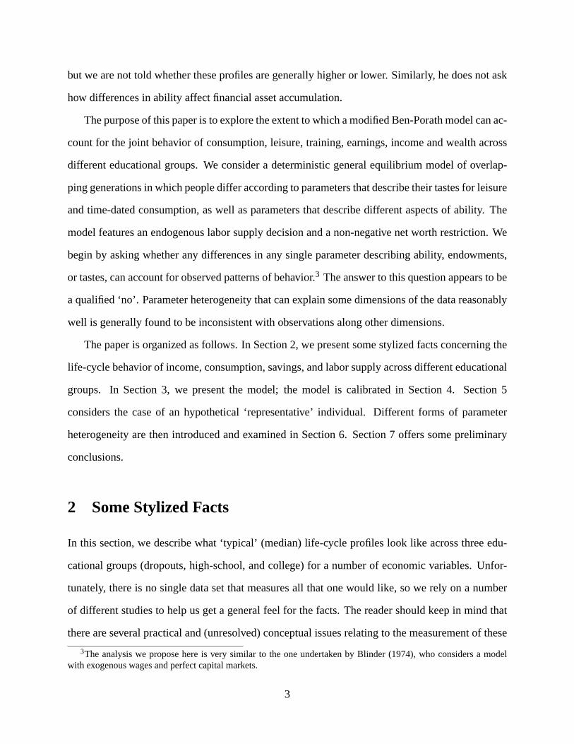
The purpose of this paper is to explore the extent to which a modified Ben-Porath model can ac-

count for the joint behavior of consumption, leisure, training, earnings, income and wealth across

different educational groups. We consider a deterministic general equilibrium model of overlap-

ping generations in which people differ according to parameters that describe their tastes for leisure

and time-dated consumption, as well as parameters that describe different aspects of ability. The

model features an endogenous labor supply decision and a non-negative net worth restriction. We

begin by asking whether any differences in any single parameter describing ability, endowments,

or tastes, can account for observed patterns of behavior.3 The answer to this question appears to be

a qualified ‘no’. Parameter heterogeneity that can explain some dimensions of the data reasonably

well is generally found to be inconsistent with observations along other dimensions.

The paper is organized as follows. In Section 2, we present some stylized facts concerning the

life-cycle behavior of income, consumption, savings, and labor supply across different educational

groups. In Section 3, we present the model; the model is calibrated in Section 4. Section 5

considers the case of an hypothetical ‘representative’ individual. Different forms of parameter

heterogeneity are then introduced and examined in Section 6. Section 7 offers some preliminary

conclusions.

2 Some Stylized Facts

In this section, we describe what ‘typical’ (median) life-cycle profiles look like across three edu-

cational groups (dropouts, high-school, and college) for a number of economic variables. Unfor-

tunately, there is no single data set that measures all that one would like, so we rely on a number

of different studies to help us get a general feel for the facts. The reader should keep in mind that

there are several practical and (unresolved) conceptual issues relating to the measurement of these

3The analysis we propose here is very similar to the one undertaken by Blinder (1974), who considers a modelwith exogenous wages and perfect capital markets.

3

variables; see Browning and Lusardi (1996) for details.

2.1 Disposable Income

In Figure 1, we plot median disposable income across three educational groups in the United

States for the year 1990.4 Not surprisingly, more highly educated individuals have significantly

more income at each age. The age-income profile for dropouts is essentially flat. Individuals with

high-school display a moderate hump-shaped age-income profile, while those with college have a

significant hump-shaped pattern.5 Consequently, income inequality across educational groups is

the greatest during the peak income ages of 41–55. Median income for college graduates in the

51–55 age group is 1.67 times that of high-school graduates in the same age group and 2.84 times

that of high-school dropouts.

2.2 Consumption

In Figure 2, we plot median consumption expenditure across educational groups; this data is from

the same survey in which the income data is recorded. Qualitatively, it appears that consumption

tracks disposable income fairly closely in the sense of sharing the same hump-shaped pattern.

This fact that has been referred to as the ‘consumption-income parallel’ (see Carroll and Summers

(1991)) and is sometimes used as an argument to reject the basic life-cycle model, which predicts a

flat age-consumption profile. Attanasio and Browning (1995) argue that the consumption-income

parallel largely reflects family-size effects. Using several years of U.K. FES data to follow cohorts

through time, they reproduce the finding that consumption and income move together over the

life-cycle. However, deflating consumption by an adult-equivalent scale renders a completely flat

life-cycle path for adjusted consumption. On the other hand, Gourinchas and Parker (1999) argue

that with their adjustments, consumption continues to display a hump-shape.

4This data is from Attanasio (1994) and is based on the 1990 Consumer Expenditure Survey.5It is important to keep in mind that this data represents a cross-section. That is, given general productivity growth,

the age-income profiles reported here do not represent the actual income profiles expected by any given individual.

4

2.3 Saving

Figure 3 plots ‘saving,’ defined here as the difference between median disposable income and

consumption measures reported above. The figure here is consistent with the well-known fact

that most households save very little; i.e., the vast bulk of the economy’s capital stock is owned

by a very small proportion of households. According to this data, high-school dropouts have on

average zero savings. By their late 20s, individuals with a high-school diploma appear to build

up their assets at a modest rate until retirement, but there is little evidence of dissaving during

retirement. College graduates, on the other hand, appear to build up their assets at relatively rapid

rate and maintain relatively high savings levels until retirement. This is the only group that appears

to undertake any significant dissaving during retirement. However, the amount of dissaving during

retirement is not enough to deplete the accumulated stock of wealth, a fact that suggests that this

group is likely to leave relatively large bequests.

The saving behavior reported in Figure 3 is broadly consistent with SCF and PSID data on

wealth accumulation patterns across educational groups. According to Cagetti (1999), median

net worth positions (including housing but abstracting from pension entitlements) are very low

and similar across individuals at age 30. While all three educational groups tend to save over the

entire life-cycle, the rate of asset accumulation is much higher for well-educated individuals. By

age 60, the median dropout has accumulated roughly between $60,000–90,000; the median high-

school graduate has between $125,000–180,000; and the median college graduate has between

$250,000–300,000.6 In other words, to a first approximation, each level of education is associated

with a doubling of net worth in old age.

2.4 Labor Supply

The Consumer Expenditure Survey examined by Attanasio (1994) also has data on labor supply

across education groups as well as across various demographic characteristics. In Figure 4, we

6The figures are in 1992 dollars. The lower bound is from the SCF; the upper bound is from the PSID.

5

report roughly what the life-cycle labor supply profile looks like for males; the corresponding

diagram for females looks qualitatively similar, but scaled down such annual hours average around

1500 during the peak earning years.7

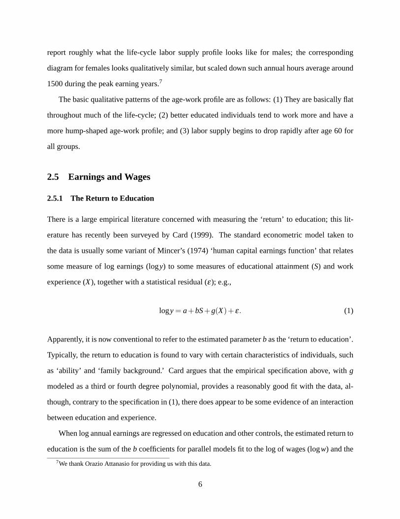
The basic qualitative patterns of the age-work profile are as follows: (1) They are basically flat

throughout much of the life-cycle; (2) better educated individuals tend to work more and have a

more hump-shaped age-work profile; and (3) labor supply begins to drop rapidly after age 60 for

all groups.

2.5 Earnings and Wages

2.5.1 The Return to Education

There is a large empirical literature concerned with measuring the ‘return’ to education; this lit-

erature has recently been surveyed by Card (1999). The standard econometric model taken to

the data is usually some variant of Mincer’s (1974) ‘human capital earnings function’ that relates

some measure of log earnings (logy) to some measures of educational attainment (S) and work

experience (X), together with a statistical residual (ε); e.g.,

logy = a+bS+g(X)+ ε. (1)

Apparently, it is now conventional to refer to the estimated parameterb as the ‘return to education’.

Typically, the return to education is found to vary with certain characteristics of individuals, such

as ‘ability’ and ‘family background.’ Card argues that the empirical specification above, withg

modeled as a third or fourth degree polynomial, provides a reasonably good fit with the data, al-

though, contrary to the specification in (1), there does appear to be some evidence of an interaction

between education and experience.

When log annual earnings are regressed on education and other controls, the estimated return to

education is the sum of theb coefficients for parallel models fit to the log of wages (logw) and the

7We thank Orazio Attanasio for providing us with this data.

6

log of annual hours (logh). Here, we reproduce Card’s (1999) Table 1, which reports the estimated

returns to education using (1) fit to the 1994–96 CPS.

Dependent Variablelogw logh logy

Menb 0.100 0.042 0.142R2 0.328 0.222 0.403

Womenb 0.109 0.056 0.165R2 0.247 0.105 0.247

Thus, Card concludes that in the U.S. labour market in the mid-1990s, about two-thirds of the

measured return to education in annual earnings data is attributable to the effect of education on

the wage rate, with the remainder attributable to the effect on annual hours worked.

3 The Model

Consider an economy populated by overlapping generations of individuals who live forJ periods,

indexed byj = 1,2, ...,J. The population is assumed to grow at a constant raten per period, and we

denote the share of age-j individuals in the population byµ j , which is time-invariant and satisfies

µ j = (1+n)µ j−1 for j = 2, ...,J and∑Jj=1 µ j = 1.

Individuals have preferences defined over deterministic time-profiles of consumptionc j , quality-

adjusted leisurezj , as well as a final net worth positionaJ+1 (bequeathed to the future generation);

let preferences be represented by the utility function:

J

∑j=1

δj−1[U(c j)+λV(zj)]+θB(aJ+1).

Assume that the functionsU , V andB are all strictly concave and that they satisfy standard Inada

conditions; we will treat these functions as common across individuals. Preferences are parame-

terized by the discount factorδ , the taste for leisureλ , and the strength of the bequest motiveθ ;

7

individuals may or may not differ along these dimensions.

There are three uses for time: market workn; learning efforte; and leisurel ; wheren+e+ l = 1

(and the usual non-negativity constraints). Leth denote human capital. People might differ in their

initial endowment of human capital (one measure of differences in ability). A person’s human

capital is assumed to augment time-use in each of the three activities; measured in ‘efficiency

units’, work effort equalhn, learning effort equalshe, and leisure outputz equalshl.

Following Heckman (1976), the human capital accumulation technology is given by:

h j+1 = (1−σ)h j +αG(h jej),

whereG is strictly increasing and concave,σ is the depreciation rate on human capital, andα

is a parameter that indexes ‘learning ability’. We will assume thatG andσ are common across

households; however,α may differ. Letv denote the vector of parameters describing a particular

individual.

There are two prices in the model. Letω denote the price of an efficiency unit of labor and

let R denote the (gross) real rate of interest. Both of these prices will be determined by market

clearing conditions in the general equilibrium. Note that labor earnings are given byωhn, so that

w = ωh can be interpreted as the real wage.

Individuals can save but cannot borrow against future earnings or bequests; consequently, all

saving is used to finance the construction of new capital. For simplicity, we assume that all bequests

accrue at some agei ∈ {1,2, ...,J} in a person’s lifetime. We also assume that type-v parents pass

on their parameter vectorv perfectly to their children (consequently, the bequest made by each

type-v individual aJ+1 will be exactly equal to the bequest receivedb at datei. Note that in the

absence of perfect capital markets, the timing of the bequest will matter. The asset accumulation

equation is given as follows:

a j+1 = Raj + χib+w jn j −c j ,

whereχi = 1 in period j = i (the period of the bequest), andχi = 0 otherwise. Optimal decision-

8

making results in a desired profile{c j ,n j ,ej , l j ,a j+1,h j+1 | b,ω,R;v}Jj=1.

Conjecture 1 There exists an unique b such that aJ+1 = b.

If the conjecture above is true, then optimal decision-making can be conditioned solely on

(ω,R;v). In the special case of zero bequests (i.e.,θ = 0), we haveaJ+1 = b= 0 and all individuals

begin life with zero net worth (this is the case we consider below). What remains now is the

determination of prices.

In a steady-state, the per capita capital stock is given by:

K = (1+n)−1J

∑j=1

µ j ∑v

a j(v)Λ(v),

whereΛ(v) represents the fraction of the population with parameter vectorv. The per capita level

of hours (measured in efficiency units) is given by:

H =J

∑j=1

µ j ∑v

h j(v)n j(v)Λ(v)

Output is produced by a constant returns to scale production technologyQ= F(K,H). Equilibrium

prices are determined by the usual marginal conditions:

ω =FH(K,H)

R=FK(K,H)+1−φ ,

whereφ is the depreciation rate of physical capital. Finally, goods-market clearing requires:

C+(n+φ)K = Q,

where,

C =J

∑j=1

µ j ∑v

c j(v)Λ(v).

9

3.1 Parameterization

Functional forms are required forU , V, B, G andF .

U(c) =c1−γ −1

1− γ

V(z) =z1−η −1

1−η

B(a) =a1−ρ −1

1−ρ

G(x) =xζ

F(K,H) =KπH1−π .

4 Calibration

At this stage, we do not have the time to calibrate or estimate the model as precisely as we would

like. So, we will content ourselves with a rough calibration. We calibrate first to a ‘representative’

individual; the parameters are chosen as follows.

4.1 Demographics

Let the number of periods beJ = 11; the length of a period is five years (think of people beginning

their economic life at age 20 and living to 70). The population growth rate is set ton = 0, so that

µ j = 1/J for all j.

4.2 Preferences

The curvature parameter onU is chosen to beγ = 1 (a standard choice). The curvature forV is

also chosen to beη = 1. We will abstract from the bequest motive; i.e.,θ = 0 (so the curvature

parameter forB does not matter). The weighting factor for leisure is chosen to beλ = 1.75; this

generates the result that roughly 1/3 of available time is devoted to the labour market. The discount

factor is chosen to beδ = 0.86, which implies an annual discount rate of 3%.

10

4.3 Technology

The learning ability parameter is set toα = 0.4; this implies that young people spend around 10%

of their available time in learning activities. The curvature of the learning technology is taken

from Heckman (1976);ζ = 0.70. The share of physical capital in total output is set toπ = 0.33.

Physical capital depreciates at an annual rate of 13.5%; setφ = 0.48. Assume that human capital

does not depreciate;σ = 0.

4.4 Endowments

The human capital endowment is normalized toh1 = 1.

5 Representative Individual

In Figure 5 we plot the life-cycle behavior of the representative individual; i.e., the equilibrium

based on the parameterization above.

As Figure 5 reveals, the model does a very nice job of replicating ‘typical’ life-cycle behavior,

with the possible exception of the very aged. In particular, the model predicts that consumption

continues to rise throughout the life-cycle; the data suggests otherwise. As well, in the model, in-

dividuals dissave in old age much more rapidly than in the data. This last feature could presumably

be rectified by incorporating the bequest motive.

6 Evaluating Alternative Sources of Heterogeneity

In this section, we consider four separate sources of heterogeneity and evaluate how each, in isola-

tion, is predicted to affect life-cycle behavior. The four parameters we consider are: (1) the ability

to learn,α; (2) the initial endowment of human capital,h1; (3) the discount factor,δ ; and (4) the

taste for leisure,λ . For each case, we will model three types, representing high, medium, and low

11

values, with 50% of the population taking on the medium value, and the other 50% evenly divided

across the two extreme values.

6.1 Heterogeneous Learning Ability

Suppose that individuals differ only in their ability to learn; e.g.,α = 0.3,0.4,0.5. The results are

plotted in Figure 6 (high ability types are associated with college graduates and low ability types

are associated with dropouts).

Observe that the earnings profiles take the expected shape in the sense that those with low

learning ability have higher earnings when young (relative to high learning ability types), and

relatively lower earnings when old. This basic qualitative pattern is also highlighted in Neal and

Rosen (2000), Figure 4.2, who remark that this U-shaped relationship between cohort earnings

variance and cohort age is an important theme in the literature on human capital.

But as Figure 6 reveals, differences in learning ability alone cannot account for life-cycle be-

havior. In particular, the model has wildly inaccurate predictions concerning the rate at which

financial assets are accumulated across education groups. According to the model, individuals

with low learning ability (dropouts) will accumulate financial assets rapidly, while those with high

learning ability (college) will not even begin accumulating assets until age 40.

The model’s logic is perfectly clear. Wealth takes two forms in this model: human wealth

and financial wealth. Low ability individuals naturally wish to substitute into the accumulation of

financial wealth, while high ability individuals allocate their resources toward accumulating human

capital. Later on in the life-cycle, those who are rich in human capital work harder to exploit their

relatively high skill levels, while those who are rich in financial wealth can afford to consume more

leisure.

12

6.2 Heterogeneous Human Capital Endowment

An alternative notion of ability is in terms of a person’s endowed human capital stock, possibly

inherited at an early age by parental teachings. Unlike learning ability, which is specific to ac-

cumulation of human capital, the ability represented in the endowed human capital stock makes

the individual more skillful in all three time uses: work, learning, and leisure. Figure 7 plots the

model’s prediction with differences in this type of ability.

According to the model, people who are born with high skill levels do not spend much time

learning (the model would associate these individuals with dropouts). The amount of time spent

learning measured inefficiency units(i.e.,eh) is very similar across different types, but the amount

of raw time spent learning is not.

The dispersion in cohort earnings is predicted to be greatest during youth, which is counterfac-

tual. Furthermore, the highly-skilled individuals work relatively hard in youth and display a steeply

declining hours-age profile; this too is counterfactual. On the positive side, the model does fairly

well at replicating consumption and asset accumulation patterns (except for the fact that ‘dropouts’

have the higher profiles).

6.3 Heterogeneous Discount Rate

The idea that people differ in their degree of ‘patience’, and that this might explain much eco-

nomic behavior, is an old one; see Rae (1834). Here we consider the three (annualized) discount

rates equal to 0.0275, 0.03 and 0.0325, corresponding to the ‘Very Patient’, the ‘Patient’, and the

‘Impatient’, respectively. The results are plotted in Figure 8.

With perfect capital markets, differences in the rate of pure time preference would have no

impact on the schooling decision.

According to Figure 8, this hypothesis actually shows some promise in replicating observed

life-cycle patterns, especially in regard to wealth accumulation. But there are some problems here

as well. In particular, as cohorts approach mid-life, the earnings of the well-educated begin to

13

drop off steeply as they come to rely more on their capital income. Earnings drop off because of

labour supply behavior; the patient have sacrificed consumption and leisure when young for higher

levels of consumption and leisure in the future. The sharp drop off in hours worked reflects the fact

that these prudent and (now) wealthy individuals can afford to consume more leisure. In the data,

however, the well-educated tend to work harder throughout the entire life-cycle.

6.4 Heterogeneous Taste for Leisure

Here we consider the hypothesis that people differ in the relative weights they place on ‘market-

based’ consumption versus ‘home-based’ consumption. Before proceeding, we should emphasize

that the framework we have adopted here is from Heckman (1976), where human capital is assumed

to be equally productive in producing either output or leisure. An alternative specification (one

which we will explore) would have human capital improving productivity only in the market sector.

The three parameter values we use areλ = 1.25,1.75,2.25, which correspond to ‘Workaholics’,

‘Normal’, and ‘Leisure-Lovers’, respectively, in Figure 9.

This hypothesis also shows some promise in explaining some patterns of behavior. In partic-

ular, the qualitative positioning of the profiles for earnings, income, hours and consumption look

not too bad, except possibly for very early on in the life cycle. However, under the specification

considered here, this hypothesis predicts identical schooling and saving behavior across the three

groups of individuals. Under the current specification, ‘lazy’ individuals are motived to accumu-

late human capital as rapidly as anyone else; the reason being that human capital augments the

production of leisure (measured in efficiency units). Again, we conjecture that by altering the

Heckman specification to the more traditional one in which human capital augments only market-

based activity (and schooling), the hypothesis of heterogeneous tastes for leisure might do very

well in replicating all patterns of life-cycle behavior reasonably well.

14

7 Preliminary Conclusions

In this paper we have reviewed some stylized facts concerning the life-cycle behavior of indi-

viduals distinguished by their human capital investments. We have attempted to interpret these

differences in the context of a modified Ben-Porath human capital model that featured individuals

who differed in the parameters that describe tastes, ability and endowments. We discovered that

no single parameter seems capable of describing the heterogeneous patterns of economic behavior

that arise in the data (an exception may turn out to be the taste for leisure parameter in a suitably

modified environment). However, there is a possibility that some combination of parameters may

do the trick and we plan an estimation exercise in order to discover whether this might be the case.

One of two things will come out of this exercise. Either we will discover that a suitably pa-

rameterized version of the human capital theory can account reasonably well for the facts, or we

will discover otherwise. In either case, we will have a valuable result. In the latter case, we will

have provided a challenge for the human capital theorists, which will presumably send them back

to the drawing board. In the former case, we can begin to use the model to explore its implications

for policy. The source of parameter heterogeneity can matter for the optimal design of policy; see

Blackorby and Donaldson (1988) and Andolfatto (2000). At this stage, it would also be appropriate

to ask the deeper questions of what exactly is it that determines differences in tastes and ability.

15

References

ANDOLFATTO, D., “A Theory of Inalienable Property Rights,” (2000), manuscript, University of

Waterloo.

ATTANASIO, O. P., “Personal Saving in the United States,” in J. M. Poterba, (ed.) “International

Comparisons of Household Saving,” (Chicago: National Bureau of Economic Research, Uni-

versity of Chicago Press) (1994) 57–123.

ATTANASIO, O. P.AND M. BROWNING, “Consumption over the Life Cycle and over the Business

Cycle,” American Economic Review85 (1995), 1118–1137.

BEN-PORATH, Y., “The Production of Human Capital and the Life Cycle of Earnings,”Journal of

Political Economy75 (1967), 352–365.

BLACKORBY, C. AND D. DONALDSON, “Cash versus Kind, Self-selection, and Efficient Trans-

fers,” American Economic Review78 (1988), 691–700.

BLINDER, A. S.,Toward an Economic Theory of Income Distribution(The MIT Press) (1974).

BLINDER, A. S. AND Y. WEISS, “Human Capital and Labor Supply: A Synthesis,”Journal of

Political Economy84 (1976), 449–472.

BROWNING, M. AND A. L USARDI, “Household Saving: Micro Theories and Micro Facts,”Jour-

nal of Economic Literature34 (1996), 1797–1855.

CAGETTI, M., “Wealth Accumulation Over the Life Cycle and Precautionary Savings,” (1999),

presented at the 1999 NBER Summer Institute.

CARD, D., “The Causal Effect of Education on Earnings,” in O. Ashenfelter and D. Card, (eds.)

“Handbook of Labor Economics,” volume 3A (Amsterdam; New York and Oxford: Elsevier

Science, North-Holland) (1999) 1801–1863.

CARROLL, C. D. AND L. H. SUMMERS, “Consumption Growth Parallels Income Growth: Some

New Evidence,” in B. D. Bernheim and J. B. Shoven, (eds.) “National Saving and Economic

16

Performance,” (Chicago: National Bureau of Economic Research, University of Chicago

Press) (1991) 305–343.

GOURINCHAS, P.-O.AND J. A. PARKER, “Consumption Over the Life Cycle,” (1999), presented

at the 1999 NBER Summer Institute.

HECKMAN , J. J., “A Life-Cycle Model of Earnings, Learning, and Consumption,”Journal of

Political Economy84 (1976), S11–44.

L ILLARD , L. A., “Inequality: Earnings vs. Human Wealth,”American Economic Review67

(1977), 42–53.

M INCER, J.,Schooling, Experience and Earnings(Columbia University Press) (1974).

NEAL , D. AND S. ROSEN, “Theories of the Distribution of Labor Earnings,” in A. B. Atkinson and

F. Bouguignon, (eds.) “Handbook of Income Distribution, Volume 1,” (Amsterdam: Elsevier)

(2000) 379–427.

RAE, J., Statement of Some New Principles on the Subject on the Subject of Political Economy

(Boston: Hilliard, Gray and Co.; reprinted by Augustus M. Kelley, Bookseller, New York

(1964)) (1834).

RYDER, H. E., F. P. STAFFORD, AND P. E. STEPHAN, “Labor, Leisure and Training over the Life

Cycle,” International Economic Review17 (1976), 651–674.

17

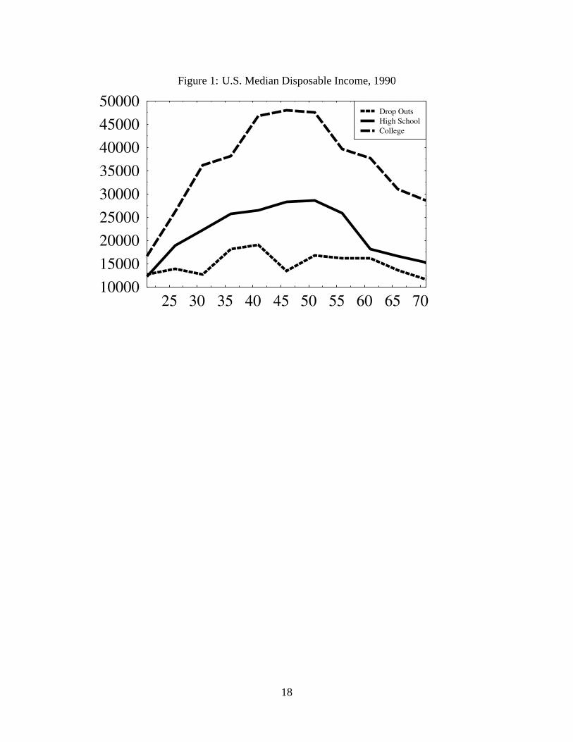
Figure 1: U.S. Median Disposable Income, 1990

25 30 35 40 45 50 55 60 65 70100001500020000250003000035000400004500050000

CollegeHigh SchoolDrop Outs

18

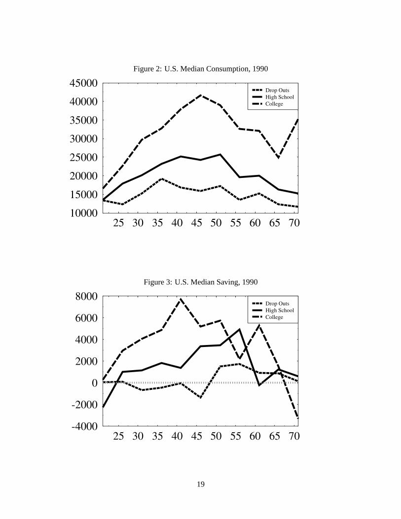
Figure 2: U.S. Median Consumption, 1990

25 30 35 40 45 50 55 60 65 7010000

15000

20000

25000

30000

35000

40000

45000


Figure 3: U.S. Median Saving, 1990

25 30 35 40 45 50 55 60 65 70-4000

-2000

0

2000

4000

6000

8000


19

Figure 4: U.S. Male Labor Supply

20 25 30 35 40 45 50 55 60 65 700

500

1000

1500

2000CollegeHigh SchoolDrop Outs

20

Figure 5: Representative Agent

1 2 3 4 5 6 7 8 9 100.1

0.12

0.14

0.16

0.18

0.2

0.22

0.24

0.26

ConsumptionEarningsIncome

1 2 3 4 5 6 7 8 9 10

0.0

0.1

0.2

0.3

0.4

Work+TrainingWork

1 2 3 4 5 6 7 8 9 101.0

1.05

1.1

1.15

1.2

1.25

Net Worth

1 2 3 4 5 6 7 8 9 100.4

0.42

0.44

0.46

0.48

0.5

0.52

0.54

Wage Rate

21

Figure 6: Differences in Learning Ability

1 2 3 4 5 6 7 8 9 100.05

0.1

0.15

0.2

0.25

0.3

CollegeHighschoolDropouts

(a) Income

1 2 3 4 5 6 7 8 9 100.0

0.05

0.1

0.15

0.2

0.25

0.3

0.35


(b) Earnings

1 2 3 4 5 6 7 8 9 100.12

0.14

0.16

0.18

0.2

0.22

0.24

0.26

0.28

0.3


(c) Consumption

1 2 3 4 5 6 7 8 9 100.1

0.15

0.2

0.25

0.3

0.35

0.4

0.45


(d) Hours Worked

1 2 3 4 5 6 7 8 9 10-0.2

-0.1

0.0

0.1

0.2

0.3


(e) Net Worth

1 2 3 4 5 6 7 8 9 100.4

0.45

0.5

0.55

0.6

0.65

0.7

0.75

0.8


(f) Wage

22

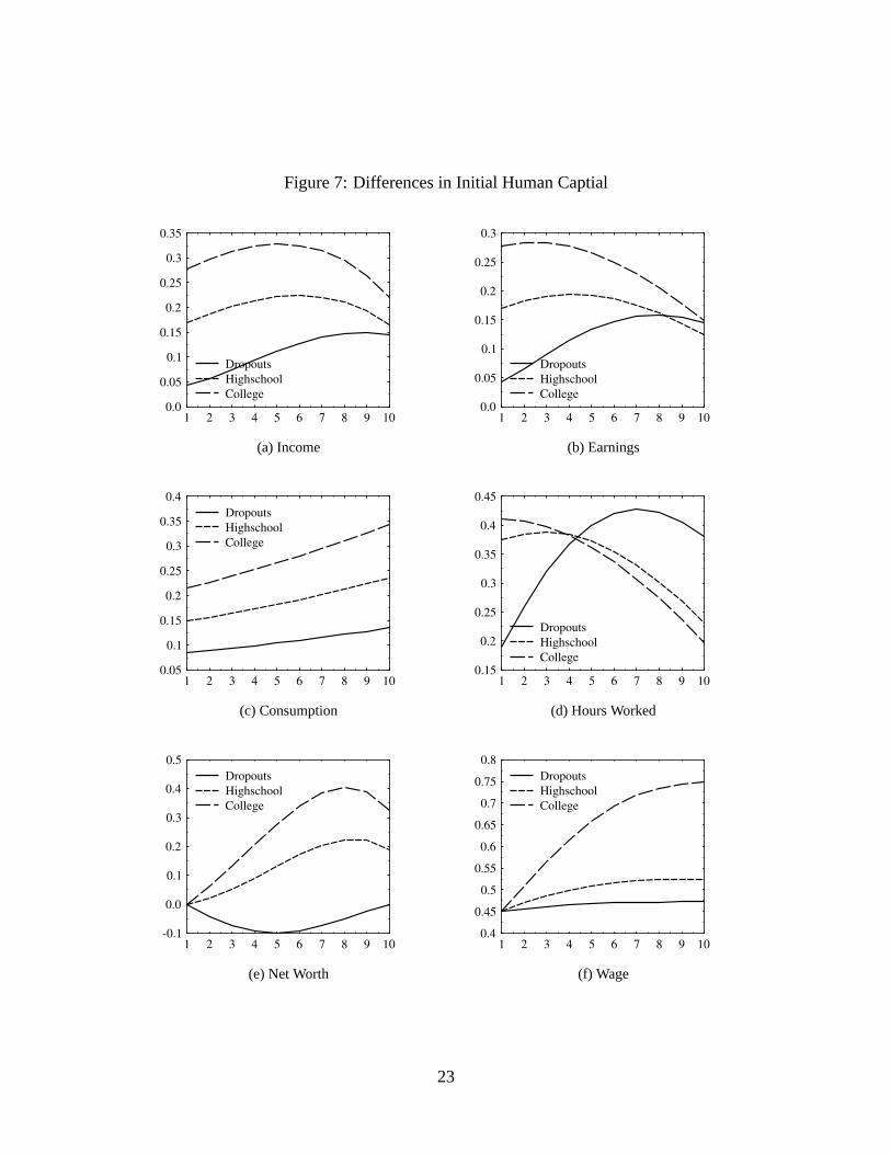
Figure 7: Differences in Initial Human Captial

1 2 3 4 5 6 7 8 9 100.0

0.05

0.1

0.15

0.2

0.25

0.3

0.35


(a) Income

1 2 3 4 5 6 7 8 9 100.0

0.05

0.1

0.15

0.2

0.25

0.3


(b) Earnings

1 2 3 4 5 6 7 8 9 100.05

0.1

0.15

0.2

0.25

0.3

0.35

0.4


(c) Consumption

1 2 3 4 5 6 7 8 9 100.15

0.2

0.25

0.3

0.35

0.4

0.45


(d) Hours Worked

1 2 3 4 5 6 7 8 9 10-0.1

0.0

0.1

0.2

0.3

0.4

0.5


(e) Net Worth

1 2 3 4 5 6 7 8 9 100.4

0.45

0.5

0.55

0.6

0.65

0.7

0.75

0.8


(f) Wage

23

Figure 8: Differences in Time-Preference

1 2 3 4 5 6 7 8 9 100.1

0.12

0.14

0.16

0.18

0.2

0.22

0.24


(a) Income

1 2 3 4 5 6 7 8 9 100.06

0.08

0.1

0.12

0.14

0.16

0.18

0.2

0.22


(b) Earnings

1 2 3 4 5 6 7 8 9 100.14

0.16

0.18

0.2

0.22

0.24

0.26

0.28


(c) Consumption

1 2 3 4 5 6 7 8 9 100.1

0.15

0.2

0.25

0.3

0.35

0.4

0.45


(d) Hours Worked

1 2 3 4 5 6 7 8 9 10-0.05

0.0

0.05

0.1

0.15

0.2

0.25

0.3

0.35


(e) Net Worth

1 2 3 4 5 6 7 8 9 100.4

0.45

0.5

0.55

0.6


(f) Wage

24

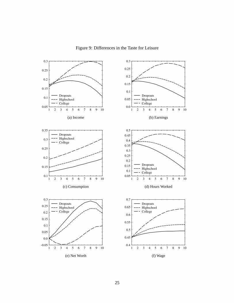
Figure 9: Differences in the Taste for Leisure

1 2 3 4 5 6 7 8 9 100.05

0.1

0.15

0.2

0.25

0.3


(a) Income

1 2 3 4 5 6 7 8 9 100.0

0.05

0.1

0.15

0.2

0.25

0.3


(b) Earnings

1 2 3 4 5 6 7 8 9 100.1

0.15

0.2

0.25

0.3

0.35


(c) Consumption

1 2 3 4 5 6 7 8 9 100.05

0.1

0.15

0.2

0.25

0.3

0.35

0.4

0.45

0.5


(d) Hours Worked

1 2 3 4 5 6 7 8 9 10-0.05

0.0

0.05

0.1

0.15

0.2

0.25

0.3


(e) Net Worth

1 2 3 4 5 6 7 8 9 100.4

0.45

0.5

0.55

0.6

0.65

0.7


(f) Wage

25

Figure 10: Negative Correlation Between the Rate of Time-Preference and the Ability to Learn

1 2 3 4 5 6 7 8 9 100.12

0.14

0.16

0.18

0.2

0.22

0.24

0.26

0.28

0.3


(a) Income

1 2 3 4 5 6 7 8 9 100.1

0.12

0.14

0.16

0.18

0.2

0.22

0.24

0.26


(b) Earnings

1 2 3 4 5 6 7 8 9 100.14

0.16

0.18

0.2

0.22

0.24

0.26

0.28

0.3

0.32


(c) Consumption

1 2 3 4 5 6 7 8 9 100.15

0.2

0.25

0.3

0.35

0.4

0.45


(d) Hours Worked

1 2 3 4 5 6 7 8 9 10-0.05

0.0

0.05

0.1

0.15

0.2

0.25

0.3


(e) Net Worth

1 2 3 4 5 6 7 8 9 100.4

0.45

0.5

0.55

0.6

0.65

0.7


(f) Wage

26

Figure 11: Positive Correlation Between the Rate of Time-Preference and the Taste for Leisure

1 2 3 4 5 6 7 8 9 100.120.140.160.180.2

0.220.240.260.28

0.30.32


(a) Income

1 2 3 4 5 6 7 8 9 100.1

0.12

0.14

0.16

0.18

0.2

0.22

0.24

0.26

0.28


(b) Earnings

1 2 3 4 5 6 7 8 9 100.1

0.15

0.2

0.25

0.3

0.35

0.4


(c) Consumption

1 2 3 4 5 6 7 8 9 100.15

0.2

0.25

0.3

0.35

0.4

0.45

0.5


(d) Hours Worked

1 2 3 4 5 6 7 8 9 10-0.05

0.0

0.05

0.1

0.15

0.2

0.25

0.3

0.35


(e) Net Worth

1 2 3 4 5 6 7 8 9 100.4

0.45

0.5

0.55

0.6


(f) Wage

27

Documents

Human Capital Theory and the Life-Cycle Pattern of ...paulgomme.github.io/lifecycle.pdf · Human Capital Theory and the Life-Cycle Pattern of Learning and Earning, Income and Wealth