Embed Size (px)
Citation preview
Hybrid Prognostic Model for Residual Useful Life Estimation of Degraded Equipment
Jie Zhang
Reliability, Availability, Maintainability and Safety (RAMS)
Supervisor: Yiliu Liu, IPK
Department of Production and Quality Engineering
Submission date: July 2015
Norwegian University of Science and Technology


RAMSReliability, Availability,
Maintainability, and Safety
Hybrid Prognostic Model for Residual Useful
Life Estimation of Degraded Equipment
JIE ZHANG
June 2015
MASTER THESIS
Department of Production and Quality Engineering
Norwegian University of Science and Technology
Supervisor: Professor Yiliu Liu

i
Preface
This is a Master’s thesis in RAMS (Reliability, Availability, Maintainability and Safety) at NTNU
as part of the study program, when it was carried out during the spring semester of 2015).
In this report, The basic concepts in prognostics and health management and different diag-
nostic and prognostic methods have been discussed. a case study of choke valve is implemented
and one hybrid model has been proposed for valve erosion.
The reader is assumed to have some basic knowledge of condition-based maintenance or
prognostics and health management.
Trondheim, 2015-06-16
Jie Zhang

ii
Acknowledgment
First, I would like to thank my professor Yiliu Liu for the patient guidance of my work and the
suggestions of my thesis structure.
In addition, I would like to thank Professor Anne Barros for giving guidance on Gamma pro-
cess. And also I would like to thank my sister who gives me advices for modeling. Moreover, I
really appreciate that Fen and Yun are often present to discuss the topics and questions what we
have met in common. Finally, I would like to thank my friends for their cheering up, encourage-
ment and support.
J.Z.
iii
Summary and Conclusions
As the consequence of the more widely used complex systems, there has been a shift in main-
tenance strategy. The traditional corrective maintenance is gradually replaced by preventive
maintenance or even more advanced philosophy such as condition based maintenance and
prognostics and health management. This thesis introduces prognostics and health manage-
ment that can implement the advanced condition-based maintenance for the more complex
and dynamic systems. First, the content of prognostics and health management is discussed,
and then the procedure is described as data acquisition, data processing, diagnostics and prog-
nostics, and maintenance decision making. In addition, historical literatures about diagnostic
and prognostic models are systematically and throughly reviewed. It consists of model-based
models and data-driven models and the paper focuses more on data-driven models, due to its
simplicity and generality. Since degradation is one of main causes for system failure either for
either machinery or electronics, degradation status assessment and prognostics are discussed
in this paper. Gamma process is suitable for monotonic degradation, but there is a prerequi-
site that the degradation indicator is observable. In order to overcome this limitation, ANNs
are used to calculate the value of indicator by monitoring relevant measurable covariates. One
hybrid model is proposed consists of ANNs model together with Gamma process for degrada-
tion prognostics. Bayesian estimation for updating the scale parameter of gamma process is
suggested to improve the accuracy.
Chock valve is studied as a case to demonstrate how the hybrid model can be applied to
estimate valve residual useful life. The case study approves the results from hybrid prognostic
model, the distribution of RUL can support the maintenance decision making. This proposed
hybrid model can not only be applied to subsea valves erosion prognostics, but also can be
applied to other equipment degradation prognostics problem.
Contents
Preface . . . . . . . . . . . . . . . . . . . . . . . . . . . . . . . . . . . . . . . . . . . . . . . . i
Acknowledgment . . . . . . . . . . . . . . . . . . . . . . . . . . . . . . . . . . . . . . . . . . ii
Summary and Conclusions . . . . . . . . . . . . . . . . . . . . . . . . . . . . . . . . . . . . iii
1 Introduction 1
1.1 Background . . . . . . . . . . . . . . . . . . . . . . . . . . . . . . . . . . . . . . . . . . 1
1.2 Objectives . . . . . . . . . . . . . . . . . . . . . . . . . . . . . . . . . . . . . . . . . . . 2
1.3 Limitations . . . . . . . . . . . . . . . . . . . . . . . . . . . . . . . . . . . . . . . . . . . 3
1.4 Approach . . . . . . . . . . . . . . . . . . . . . . . . . . . . . . . . . . . . . . . . . . . . 3
1.5 Structure of the report . . . . . . . . . . . . . . . . . . . . . . . . . . . . . . . . . . . . 4
2 Introduction of prognostics and health management 5
2.1 Evolution of maintenance technologies . . . . . . . . . . . . . . . . . . . . . . . . . . 5
2.2 Content of Prognostics and Health Management . . . . . . . . . . . . . . . . . . . . 7
2.3 Procedure of PHM . . . . . . . . . . . . . . . . . . . . . . . . . . . . . . . . . . . . . . 9
2.3.1 FMECA analysis . . . . . . . . . . . . . . . . . . . . . . . . . . . . . . . . . . . . 9
2.3.2 Data Acquisition . . . . . . . . . . . . . . . . . . . . . . . . . . . . . . . . . . . 9
2.3.3 Data processing . . . . . . . . . . . . . . . . . . . . . . . . . . . . . . . . . . . . 10
2.3.4 Diagnostics . . . . . . . . . . . . . . . . . . . . . . . . . . . . . . . . . . . . . . 11
2.3.5 Prognostics . . . . . . . . . . . . . . . . . . . . . . . . . . . . . . . . . . . . . . 12
2.3.6 Decision making . . . . . . . . . . . . . . . . . . . . . . . . . . . . . . . . . . . 13
2.4 Diagnostics methods review . . . . . . . . . . . . . . . . . . . . . . . . . . . . . . . . . 13
2.4.1 Model-based approaches . . . . . . . . . . . . . . . . . . . . . . . . . . . . . . 13
2.4.2 Data-driven approaches . . . . . . . . . . . . . . . . . . . . . . . . . . . . . . . 14
iv

CONTENTS v
2.5 Prognostics methods review . . . . . . . . . . . . . . . . . . . . . . . . . . . . . . . . . 15
2.5.1 Experience-based prognostics approaches . . . . . . . . . . . . . . . . . . . . 16
2.5.2 Data-driven method . . . . . . . . . . . . . . . . . . . . . . . . . . . . . . . . . 17
2.5.3 Model based method . . . . . . . . . . . . . . . . . . . . . . . . . . . . . . . . . 21
3 Proposed hybrid model for degradation prognostics 23
3.1 Propose a hybrid model . . . . . . . . . . . . . . . . . . . . . . . . . . . . . . . . . . . 24
3.2 Artificial Neural Network . . . . . . . . . . . . . . . . . . . . . . . . . . . . . . . . . . . 25
3.2.1 Feedforward neural network . . . . . . . . . . . . . . . . . . . . . . . . . . . . 27
3.2.2 NNs merits and limitations . . . . . . . . . . . . . . . . . . . . . . . . . . . . . 29
3.3 Stochastic Process . . . . . . . . . . . . . . . . . . . . . . . . . . . . . . . . . . . . . . 30
3.3.1 Parameter Estimation . . . . . . . . . . . . . . . . . . . . . . . . . . . . . . . . 32
3.3.2 Estimation of RUL . . . . . . . . . . . . . . . . . . . . . . . . . . . . . . . . . . 33
3.3.3 Merits and Limitations . . . . . . . . . . . . . . . . . . . . . . . . . . . . . . . . 34
4 Hybrid model application on subsea valves 35
4.1 Subsea choke valves introduction . . . . . . . . . . . . . . . . . . . . . . . . . . . . . 35
4.2 Choke valve erosion . . . . . . . . . . . . . . . . . . . . . . . . . . . . . . . . . . . . . 36
4.3 Hybrid model for choke RUL estimation . . . . . . . . . . . . . . . . . . . . . . . . . 38
4.4 Visualization of the erosion indicator . . . . . . . . . . . . . . . . . . . . . . . . . . . 38
4.4.1 Calculating δCv . . . . . . . . . . . . . . . . . . . . . . . . . . . . . . . . . . . . 38
4.4.2 Filtering of δCv . . . . . . . . . . . . . . . . . . . . . . . . . . . . . . . . . . . . 40
4.4.3 Building ANNs model . . . . . . . . . . . . . . . . . . . . . . . . . . . . . . . . 42
4.5 Gamma process parameter estimation . . . . . . . . . . . . . . . . . . . . . . . . . . 43
4.5.1 Maximum likelihood method . . . . . . . . . . . . . . . . . . . . . . . . . . . . 43
4.5.2 Bayesian method for updating u . . . . . . . . . . . . . . . . . . . . . . . . . . 46
4.6 Residual useful life Prediction . . . . . . . . . . . . . . . . . . . . . . . . . . . . . . . . 48
5 Summary 52
5.1 Summary and conclusions . . . . . . . . . . . . . . . . . . . . . . . . . . . . . . . . . 52
5.2 Discussion . . . . . . . . . . . . . . . . . . . . . . . . . . . . . . . . . . . . . . . . . . . 53
5.3 Recommendations for further work . . . . . . . . . . . . . . . . . . . . . . . . . . . . 53

CONTENTS vi
A Acronyms 55
B 57
B.1 ANNs . . . . . . . . . . . . . . . . . . . . . . . . . . . . . . . . . . . . . . . . . . . . . . 57
B.2 Choke A . . . . . . . . . . . . . . . . . . . . . . . . . . . . . . . . . . . . . . . . . . . . . 58
B.3 Choke B . . . . . . . . . . . . . . . . . . . . . . . . . . . . . . . . . . . . . . . . . . . . . 58
Bibliography 63
Curriculum Vitae 68
Chapter 1
Introduction
1.1 Background
During the past half century, more and more complex and highly embedded and automated
systems has been used in industries. The cost of unavailability of these systems is so huge that
no one can afford and in addition, the high reliability and availability of systems are the key to
ensure the safety and environment are protected. The simplest maintenance strategy (run to
failure) is out of date for the complex system. The scheduled preventive maintenance is also
not economically wise to implement since it may lead to waste of components or subsystems
useful life. As the maintenance cost accounts more and more of the operational cost, the need
to lower the maintenance cost and at the same time without compromising safe operation is in
emergency.
Condition-based maintenance has developed to minimize the unnecessary preventive main-
tenance by assessing actual equipments or components health condition based on real-time
sensor data analysis. A lot of effort has been put on failure or fault detection and diagnostics,
and the principle of diagnostics is once the monitored indicator reaches the presetting thresh-
old, system will send alarms to inform there is something wrong within the system. Based on
the diagnostic techniques, the prognostics-related techniques like fault propagation and resid-
ual useful life estimation of the system or components have only recently attracted attentions in
research studies. While according to Li and Nilkitsaranont (2009), making accurate prognostic
predictions allows benefits such as advanced scheduling of maintenance activities, proactive al-
1
CHAPTER 1. INTRODUCTION 2
location of replacement parts and enhanced fleet deployment decisions based on the estimated
progression of component life consumption.
In military and aerospace, Prognostics and health management (PHM) has been developed
as a system that can implement the advanced condition-based maintenance strategy and focus
more on prognostics and predicting the residual life. PHM has already been used in the aircraft
(Carl S. Byington et al. (2004))and military for decades, and the benefits of apply PHM is ap-
parent and remarkable. For example, the capability allows end users to improve fault isolation,
better plan maintenance, reduce or eliminate inspections, and decrease time-based mainte-
nance intervals with confidence, as well as an overall decrease in life cycle costs. Whilst in other
industries PHM is still not applied widely. For example, oil and gas industry already starts to im-
plement condition monitoring technologies to monitor the equipments’ degradation, but the
prognostics has not even been considered as one necessary practice. Considering the more time
consuming and difficult maintenance for subsea equipments, it is imperative to apply prognos-
tic algorithms in subsea industry to calculate the residual useful life (RUL) of the equipments,
which can let the proactive maintenance practicable. Prognostics and health management is
a wide topic and in this paper the main focus is the prognostic algorithms used in prognostics
and health management systems.
The book George Vachtsevanos (2006) details the technologies in CBM and PHM that have
been introduced by researchers and practitioners within different application domains. It con-
tains the important concepts within this field, the data collection and processing techniques,
and the diagnostics and prognostics methods. The diagnostics and prognostics methods will be
reviewed in detail in Chapter 2 in this thesis.
1.2 Objectives
The main objective is to study prognostics methods that can be used in Prognostics and Health
Management for predicting the residual useful life which can help the maintenance scheduling.
Using a subsea choke valve as a case study to discuss how can different methods be combined
together.
The sub-objectives are:
CHAPTER 1. INTRODUCTION 3
1. Summarize the prognostics and health management content and procedure;
2. Discuss different diagnostics and prognostics methods used in Prognostics and Health
Management;
3. Propose a hybrid model for dealing with the equipments degradation problem;
4. Apply the hybrid model for prognostics of choke valve erosion.
1.3 Limitations
1. This thesis focus on prognostics models more than diagnostics, and it just gives a sum-
mary for different diagnostics methods. More deep understanding of diagnostics will help
to understand prognostics better since prognostic models is developed based on diagnos-
tics;
2. The report has discussed more about the machinery prognostics, the prognostics of elec-
tronics is not covered.
3. Due to time limitation and lacking of relevant knowledge, some relevant topics have not
been introduced in detail, such as signal processing techniques, the system level health
assessment.
4. Since no field data for the case study of choke erosion, the manually generated data is
used for calculation.
1.4 Approach
The background knowledge about prognostics and health management is obtained by literature
review, and in addition the most currently common used diagnostics and prognostics method
are also reviewed. For choke valve erosion, Gamma process could be suitable method for ero-
sion prognostics and residual useful life prediction, if the limitation of Gamma process can be
solved. By compare the merits and limits of different models, ANNs model is chosen to solve the
limitation of Gamma process together with data processing techniques.

CHAPTER 1. INTRODUCTION 4
1.5 Structure of the report
The report is structured as:
• Chapter 1 introduces the background of Prognostics and health management and objec-
tives of this report;
• Chapter 2 gives a detailed introduction of the content of Prognostics and health manage-
ment and a literature review of the relevant diagnostic and prognostic models;
• A hybrid prognostics model is proposed for the equipment degradation in Chapter 3 and
the details about the ANNs model and Stochastic model are discussed;
• Chapter 4 introduces subsea choke valve as a case study, and demonstrates the hybrid
prognostic model for valve erosion;
• Chapter 5 presents the summary and conclusion of the report and recommends the future
works.
Chapter 2
Introduction of prognostics and health
management
2.1 Evolution of maintenance technologies
The earliest maintenance techniques is basically breakdown maintenance (also called correc-
tive maintenance or run-to-failure), where no actions are taken to maintain the equipment until
it breaks and consequently needs a repair or replacement. Breakdown maintenance only applies
to the equipment that is not expensive and the failure does not lead to a severe consequence.
In the 1950s, preventive maintenance (planned maintenance) was introduced to prevent the
catastrophic failures, which means regular inspections and maintenance is implemented in
certain intervals regardless of the condition of the equipment. Bazovsky (1961) pioneers the
use of mathematical optimization methods in preventive maintenance policies. Jardine (1973)
introduces decision models for determining optimal replacement or overhaul interval by ana-
lyzing reliability data (e.g. historical breakdown events) and cost data. These polices do reduce
some failures, but they can not eliminate all the catastrophic failures and at the same time it
needs more labor or sometime is more costly. Both preventative and corrective maintenance
approaches have financial implications with them. The use of conservative failure rate to de-
cide the maintenance interval will result in components regularly being replaced away before
they actually reached their end of life time. Alternatively, the use of corrective maintenance ap-
proaches makes the best use of the components serviceable time, however, the failure of com-
5
CHAPTER 2. INTRODUCTION OF PROGNOSTICS AND HEALTH MANAGEMENT 6
ponents can cause damage to other part of a system, resulting in significant repair cost and
down time cost. The common factor making them unsuitable is that the actual condition of the
equipment is not considered.
As system and equipment become more complex and expensive, the cost of the failure of sys-
tems and corresponding cost such as down time cost and safety cost is significantly increased.
In addition, high availability and reliability of the system becomes more demanding than ever.
These factors drive the industries to look for a new maintenance philosophy. Eventually, condition-
based maintenance(CBM) starts to play a role in different industries. CBM is a maintenance
program that recommends maintenance actions based on the information collected through
condition monitoring and only when there is evidence of abnormal behaviors in the equipment.
ISO (2012) defines condition monitoring (CM) as the process of monitoring a parameter of con-
dition in machinery (vibration, temperature etc.), in order to identify a significant change which
is indicative of a developing fault.
Condition-based maintenance is a kind of proactive maintenance. Compared with tradi-
tional reactive maintenance, it can not only improve operational availability, but also reduce
the unnecessary scheduled maintenance cost, reduce the spare parts inventory cost, and mini-
mize the life-cycle cost. However it can not be applied to every system. CBM can be applied in
systems that (1) can be regarded as being deterministic to some extent. (2) is stationary or static,
and (3) for which signal variables that can be good health indicators can be extracted.
With the development and advancement in censoring technology, data collection storage
and processing capabilities, and continuous improvements in algorithms and data analysis tech-
niques, CBM approaches is developing and improving. Currently, more and more focus has
shifted to prognostics and health management which focus more on incipient failure detec-
tion, current health assessment and remaining useful life prediction. Figure 2.1 illustrates the
relationship between CBM and PHM. According to Kalgren et al. (2006), PHM is a health man-
agement approach utilizing measurements, models, and software to perform incipient fault de-
tection, condition assessment, and failure progression prediction. Lee et al. (2014) considers
PHM as an evolved form of CBM, and CBM techniques can be used as input for the prognostics
models in PHM and support the timely, accurate decision making.
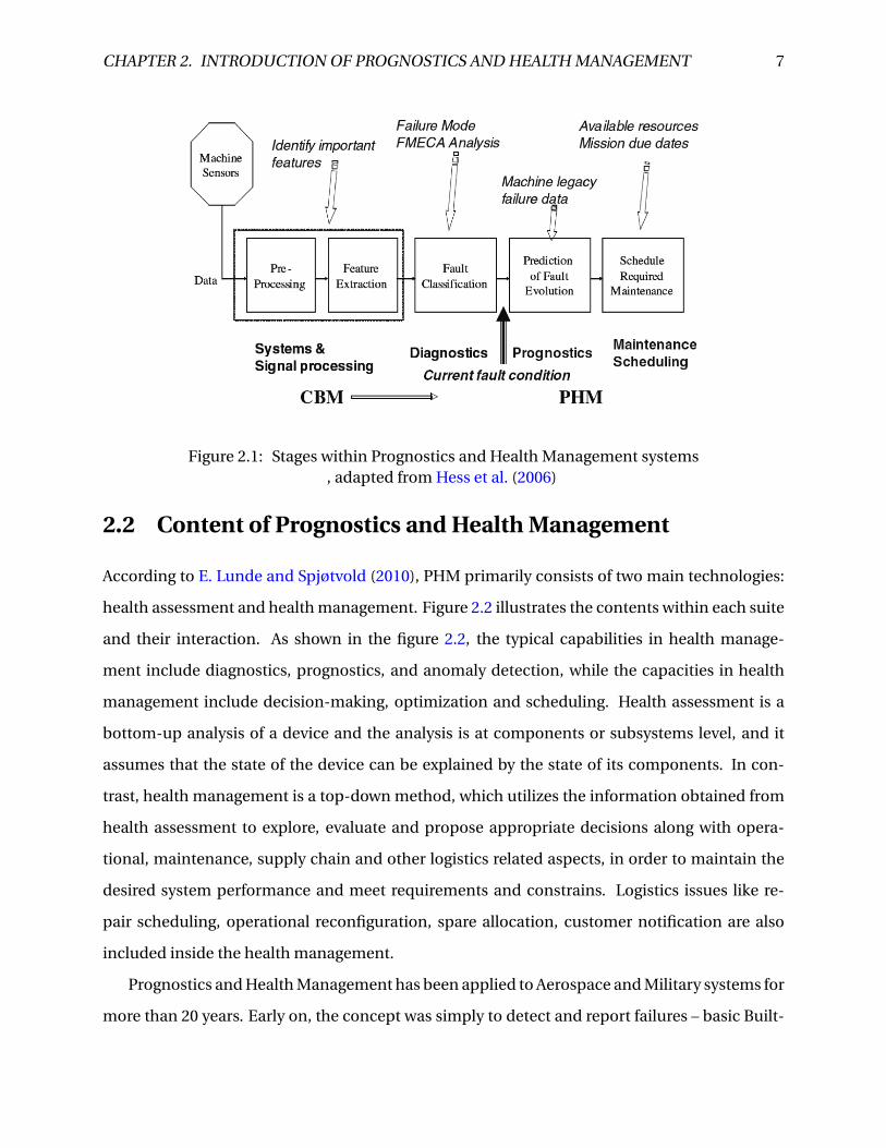
CHAPTER 2. INTRODUCTION OF PROGNOSTICS AND HEALTH MANAGEMENT 7
Figure 2.1: Stages within Prognostics and Health Management systems, adapted from Hess et al. (2006)
2.2 Content of Prognostics and Health Management
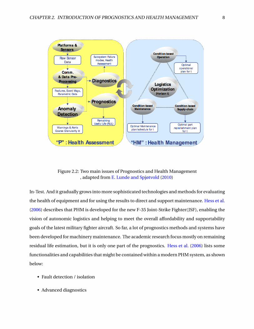
According to E. Lunde and Spjøtvold (2010), PHM primarily consists of two main technologies:
health assessment and health management. Figure 2.2 illustrates the contents within each suite
and their interaction. As shown in the figure 2.2, the typical capabilities in health manage-
ment include diagnostics, prognostics, and anomaly detection, while the capacities in health
management include decision-making, optimization and scheduling. Health assessment is a
bottom-up analysis of a device and the analysis is at components or subsystems level, and it
assumes that the state of the device can be explained by the state of its components. In con-
trast, health management is a top-down method, which utilizes the information obtained from
health assessment to explore, evaluate and propose appropriate decisions along with opera-
tional, maintenance, supply chain and other logistics related aspects, in order to maintain the
desired system performance and meet requirements and constrains. Logistics issues like re-
pair scheduling, operational reconfiguration, spare allocation, customer notification are also
included inside the health management.
Prognostics and Health Management has been applied to Aerospace and Military systems for
more than 20 years. Early on, the concept was simply to detect and report failures – basic Built-
CHAPTER 2. INTRODUCTION OF PROGNOSTICS AND HEALTH MANAGEMENT 8
Figure 2.2: Two main issues of Prognostics and Health Management, adapted from E. Lunde and Spjøtvold (2010)
In-Test. And it gradually grows into more sophisticated technologies and methods for evaluating
the health of equipment and for using the results to direct and support maintenance. Hess et al.
(2006) describes that PHM is developed for the new F-35 Joint-Strike Fighter(JSF), enabling the
vision of autonomic logistics and helping to meet the overall affordability and supportability
goals of the latest military fighter aircraft. So far, a lot of prognostics methods and systems have
been developed for machinery maintenance. The academic research focus mostly on remaining
residual life estimation, but it is only one part of the prognostics. Hess et al. (2006) lists some
functionalities and capabilities that might be contained within a modern PHM system, as shown
below:
• Fault detection / isolation
• Advanced diagnostics

CHAPTER 2. INTRODUCTION OF PROGNOSTICS AND HEALTH MANAGEMENT 9
• Predictive prognostics
• RUL and time-to-failure predictions
• Component life usage tracking
• Warranty guarantee tracking
• Health reporting and information management
• Utilization tracking
• Decision support systems
• Fault accommodation
• Information fusion and reasoners
2.3 Procedure of PHM
2.3.1 FMECA analysis
The fist step of PHM system development is to implement a comprehensive FMECA study. The
objective is to relate failures to the root causes. Through FMECA studies, all potential failure
modes, the severity of them and the probabilities of occurrence, the fault symptoms and the
monitoring methods and sensors required will be covered in the analysis at component level or
subsystem level.
Butler (2012) claims that FMECA are often used as the starting point of development of fault
diagnostics capabilities, and it typically requires input from variety of sources including domain
experts, maintenance personnel, equipment specialists and designers.
2.3.2 Data Acquisition
According to Jardine et al. (2006) data acquisition is a process of collecting and storing useful
data(information) and it is an essential step for fault diagnostics and prognostics. And Data
could be categorized into two types, namely event data and condition monitoring data. Event

CHAPTER 2. INTRODUCTION OF PROGNOSTICS AND HEALTH MANAGEMENT 10
data includes the information on what happened and what was done to the systems or equip-
ments. while condition monitoring data can be the measurements related to the condition of
the equipment. In practice, event data always need manual data entry to the information sys-
tems and sometimes may be neglected by personnel, but event data and condition monitoring
data are equally important.
With the rapid development of the computer and sensor technologies, more and more pow-
erful data acquisition techniques is becoming affordable. The most common monitoring data
can be vibration data, acoustic data, oil analysis data, temperature, pressure, humidity, mois-
ture, weather or environment data, etc. Various sensors have been designed for data collec-
tion, such as micro-sensors, ultrasonic sensors, acoustic emission sensors. This thesis will not
cover the detail about data acquisition techniques, but books like Nikolay V. Kirianaki (2002)
and Austerlitz (2002) will provide more details.
2.3.3 Data processing
Data cleaning
The first step of data processing is data cleaning. This is an important step since data, especially
event data, which is usually entered manually, always contains errors. Data cleaning ensures, or
at least increases the chance, that clean (error-free) data are used for further analysis and mod-
eling. Data errors are caused by many factors including the human factor and sensor faults. In
general, however, there is no simple way to clean data. Sometimes it requires manual examina-
tion of data. Graphical tools would be very helpful to finding and removing data errors. Data
cleaning is, indeed, a big area. It is not in the scope and will not be discussed in detail here.
Data analysis
The next step of data processing is data analysis. Jardine et al. (2006) categorizes condition
monitoring data into three categories: value type, waveform type, and multi dimension type.
Value type data is single value, like temperature, pressure, etc. Waveform data is like vibration
signals and acoustic emissions, motor current, partial discharge, etc. An example for multidi-
mensional type data is the image data. A variety of models, algorithms and tools are available in

CHAPTER 2. INTRODUCTION OF PROGNOSTICS AND HEALTH MANAGEMENT 11
the literature to analyze data for better understanding and interpretation of data. The models,
algorithms and tools used for data analysis depend mainly on the types of data collected. For
example, for waveform data analysis, frequency-domain analysis obtained by transformation
from time domain, can easily identify and isolate certain frequency components of interest. For
detail introduction about time-domain, frequency domain and time frequency analysis meth-
ods, check the article Jardine et al. (2006).
2.3.4 Diagnostics
Fault diagnostic, according to George Vachtsevanos (2006), is the foundation of the condition-
based maintenance, and it is designed to detect system performance, monitor degradation lev-
els, and identify faults based on physical property changes, through detectable phenomena.
Early diagnostic was developed in the form of built-in-test(BIT) equipment in the aircraft.
Built-in test is defined as an on-board hardware-software diagnostic means to identify and lo-
cate faults, and includes error detection and correction circuits. Later on fault diagnostic ca-
pability has bee improved due to the continuous improvement in computer power and data
storage capabilities.
The term fault diagnostics is used to describe a range of tasks and capabilities and it has not
yet been well defined. The following definition is given by George Vachtsevanos (2006):
Z Fault diagnosis: Detecting, isolating, and identifying an impending or incipient failure condition-
the affected component (subsystem, or system) is still operational even though at a degraded
mode.
Failure diagnosis: Detecting, isolating, and identifying a component (subsystem, or system)
that has ceased to operate.
Fault (failure) detection involves identifying the occurrence of a fault, or failure, in a mon-
itored system, or the identification of abnormal behavior which may be indicative of a fault
condition.
Fault (failure) isolation involves identifying which component/subsystem/system has a fault
condition, or has failed.
Fault (failure) identification involves determining the nature and extent of a system fault

CHAPTER 2. INTRODUCTION OF PROGNOSTICS AND HEALTH MANAGEMENT 12
condition or failure.
2.3.5 Prognostics
Diagnostics is conducted to investigate or analyze the cause or nature of a condition situation
or problem, whereas prognostics is concerned with calculating or predicting the future as a re-
sult of rational study and analysis of available data. Prognostics has the ability to identify the
presence of incipient fault conditions and incipient faults identification enables maintenance
personnel to potentially avoid the catastrophic failures. Butler (2012) considers prognostics as
a more difficult task than diagnostics since evolution of equipment fault conditions is subject
to stochastic processes and in addtion prognostics involves a large degree of uncertainty. The
figure 2.3 describes a clear relationship between diagnostics and prognostics according to the
propagation of the fault.
Figure 2.3: Diagnostics and Prognostics, adapted from Lee et al. (2014)
The standard ISO 13381-1 introduces a definition of prognostics, which is an estimation of
time to failure and risk for one or more existing and future failure modes. The most common
prognostics is to predict how much time left before a failure (or a fault) occurs given the current
machine condition and past operation profile. The time left before failure is called remaining
useful life(RUL). Except for RUL prediction, the probability that the machine can survive until

CHAPTER 2. INTRODUCTION OF PROGNOSTICS AND HEALTH MANAGEMENT 13
next inspection given the current condition and history operation profiles is also a good refer-
ence for maintenance personnel to make decisions.
2.3.6 Decision making
the results from prognostics such as residual useful life with its confidence level and the prob-
ability of failure before next inspection is the vital information for supporting the maitnenacen
decision making. Except for that, there are also other issue should be taken into considera-
tion, such as the availability of spare parts and specific tools, human resources, economic costs,
maintenance strategy, regulations and laws, etc. Hence, a robust maintenance decision making
system is needed to balance the different profits and boundaries. Jardine et al. (2001) introduces
the EXAKT software for optimizing maintenance decisions for the mine haul truck wheel mo-
tors. EXAKT not only considers the results from prognostics but also considers the cost function,
replacement policy, hazard sensitivity and cost sensitivity for making decision.
2.4 Diagnostics methods review
As discussed in last section diagnostics is the basis of prognostics and has been deeply re-
searched. In this section common diagnostics methods that has used are briefly reviewed, and
more focus is given to prognostics. According to George Vachtsevanos (2006) fault diagnosis
methods can be classified into two types, model-based and data-based approaches. In the fol-
lowing both two types will be introduced.
2.4.1 Model-based approaches
Model-based fault diagnostic approaches utilize a mathematical model of the system under ob-
servation. The estimated results generated by the model are then compared with the actual pro-
cess outputs, and the potential fault conditions are identified based on the residual value. The
model being utilized is derived from fist principles, and embodied by series of dynamic equa-
tions that define relationships, at a given time or load cycle, between damage (or degradation) of
a system or component and environmental and operational conditions under which the system

CHAPTER 2. INTRODUCTION OF PROGNOSTICS AND HEALTH MANAGEMENT 14
or component are operated. Figure 2.4 illustrates the basic concepts of a typical model-based
approach to fault diagnostics.
Figure 2.4: Model-based Diagnostic Approach
As illustrated in figure 2.4, a residual is generated after the comparison of actual system out-
put and the model estimate. For normal operation, the value of residual signal should be ap-
proximately zero, while when the value of the residual signal is deviated from zero, the residual
signal will be forwarded to a decision logic routine which is used to map the behavior of the
residual signal onto a specific fault condition.
2.4.2 Data-driven approaches
The general principle of data-driven approaches to fault diagnostics is to utilize pattern recogni-
tion techniques to map data in the measurement, or feature, space, to equipment faults within
the fault space. And data-driven approaches is categorized into two types, namely statistical
approaches and artificial intelligence based approaches by Jardine et al. (2006).
Statistical approaches has some common methods, such as statistical process control(SPC),
principal component analysis(PCA), and partial least squares(PLS).
CHAPTER 2. INTRODUCTION OF PROGNOSTICS AND HEALTH MANAGEMENT 15
Statistical process control, SPC, which was originally developed in quality control theory, has
been well developed and widely used in fault detection and diagnostics. The principle of SPC is
to measure the deviation of the current signal from a reference signal representing the normal
condition to see whether the current signal is within the control limits or not. Gallagher et al.
(1997) uses SPC for semiconductor chamber damage detection
Principal component analysis, PCA, is often applied to high-dimensional datasets to trans-
form a number of related variables to a smaller set of uncorrelated variables. According to
Venkatasubramanian et al. (2003), the basic principle of PCA for fault diagnostics is to derive
a PCA model using a dataset of normal fault-free behavior. Future observations are then com-
pared with this model using statistical measures such as the T 2 and Q statistics. If the measured
statistics exceed a defined limit, a potential fault condition is flagged.
Partial least squares, PLS, is a multivariate regression algorithm based upon PCA. Whilst
PCA is concerned with decomposing an input matrix X into its principal components, PLS is
concerned with developing a linear regression model by first projecting the input matrix X and
output matrix Y onto a lower dimensional space. Qin (2009) gives a contemporary review of
applications of PCA and PLS to fault diagnostics.
Cluster analysis, as a multivariate statistical analysis method, is a statistical classification ap-
proach that groups signals into different fault categories on the basis of the similarity of the char-
acteristics or features they possess. It seeks to minimize within-group variance and maximize
between-group variance. The result of cluster analysis is a number of heterogeneous groups
with homogeneous contents: There are substantial differences between the groups, but the sig-
nals within a single group are similar.
AI approaches for diagnostics includes artificial neural networks(ANNs), support vector clas-
sification, and fuzzy logic. And the detail of ANNs will be discussed in next section.
2.5 Prognostics methods review
Due to the variety of techniques that are applied into prognostics problems, it is not easy to
categorize different approaches into different classes. George Vachtsevanos (2006) categorizes
prognostics approaches into three classes, experience-based, data-driven and model-based ap-
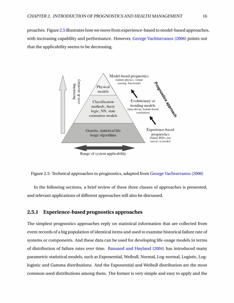
CHAPTER 2. INTRODUCTION OF PROGNOSTICS AND HEALTH MANAGEMENT 16
proaches. Figure 2.5 illustrates how we move from experience-based to model-based approaches,
with increasing capability and performance. However, George Vachtsevanos (2006) points out
that the applicability seems to be decreasing.
Figure 2.5: Technical approaches to prognostics, adapted from George Vachtsevanos (2006)
In the following sections, a brief review of these three classes of approaches is presented,
and relevant applications of different approaches will also be discussed.
2.5.1 Experience-based prognostics approaches
The simplest prognostics approaches reply on statistical information that are collected from
event records of a big population of identical items and used to examine historical failure rate of
systems or components. And these data can be used for developing life-usage models in terms
of distribution of failure rates over time. Rausand and Høyland (2004) has introduced many
parametric statistical models, such as Exponential, Weibull, Normal, Log-normal, Logistic, Log-
logistic and Gamma distributions. And the Exponential and Weibull distribution are the most
common used distributions among them. The former is very simple and easy to apply and the
CHAPTER 2. INTRODUCTION OF PROGNOSTICS AND HEALTH MANAGEMENT 17
later has the ability to adjust to varies types of failure rate in different phases, like infant, mature,
wear out phases.
The conventional experience-based approach is used for preventive maintenance schedul-
ing based on the mean time between failure(MTBF). However, these approaches do not have
predictive capability and are not the real prognostics techniques. In general, these approaches
can be applied widely in systems or components with low criticality and cost, or in the situation
where the sensor data is not available. The following data-driven and model-based methods are
developed for individual component or system prognostics.
2.5.2 Data-driven method
Data-driven approaches attempt to derive models directly from routinely collected condition
monitoring data instead of building models based on comprehensive system physics and hu-
man expertise. They are built based on historical records and produce prediction outputs di-
rectly in terms of CM data, so that it only needs the certain amount of data, and it does not
require comprehensive understanding of the system . However, the main drawback of this ap-
proach is that its effectiveness and accuracy is highly dependent on the quantity and quality of
operational data used to build the model. While, data driven models are considered to be the
most popular method for prognostics.
Data driven approach can be divided into three major categories: Artificial Intelligent (AI)
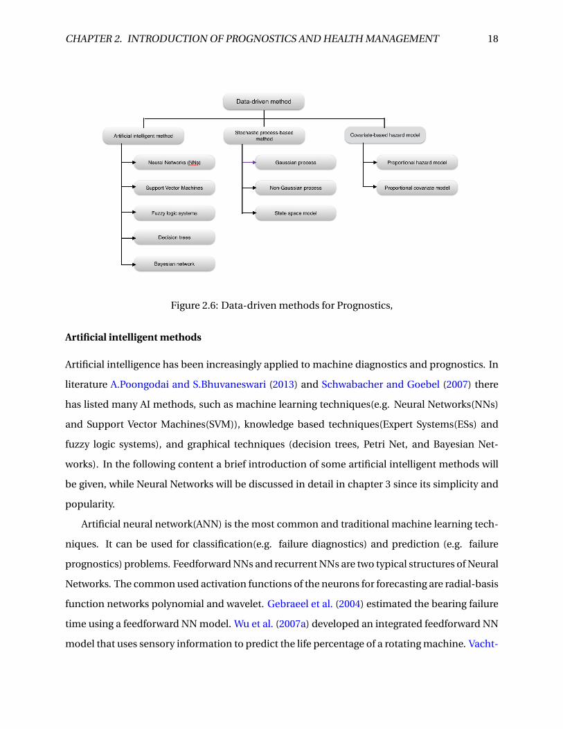
methods; stochastic process based models; and covariate based hazard models. Figure 2.6 lists
most of the date-driven method for prognostics.
Time series approaches
The conventional data-driven methods rely on simple projection models, which project the
current level of degradation into the future. Such common used approaches can be exponen-
tial smoothing techniques (Byington and Roemer (2002)) and autoregressive model (Wu et al.
(2007b)). One major advantage of these techniques is the simplicity of their calculations, which
can be carried out on a programmable calculator. However, the limitation of these trend fore-
casting techniques is the assumption of some underlying stability in the monitored system and
relying on past patterns of degradation to project future degradation.
CHAPTER 2. INTRODUCTION OF PROGNOSTICS AND HEALTH MANAGEMENT 18
Figure 2.6: Data-driven methods for Prognostics,
Artificial intelligent methods
Artificial intelligence has been increasingly applied to machine diagnostics and prognostics. In
literature A.Poongodai and S.Bhuvaneswari (2013) and Schwabacher and Goebel (2007) there
has listed many AI methods, such as machine learning techniques(e.g. Neural Networks(NNs)
and Support Vector Machines(SVM)), knowledge based techniques(Expert Systems(ESs) and
fuzzy logic systems), and graphical techniques (decision trees, Petri Net, and Bayesian Net-
works). In the following content a brief introduction of some artificial intelligent methods will
be given, while Neural Networks will be discussed in detail in chapter 3 since its simplicity and
popularity.
Artificial neural network(ANN) is the most common and traditional machine learning tech-
niques. It can be used for classification(e.g. failure diagnostics) and prediction (e.g. failure
prognostics) problems. Feedforward NNs and recurrent NNs are two typical structures of Neural
Networks. The common used activation functions of the neurons for forecasting are radial-basis
function networks polynomial and wavelet. Gebraeel et al. (2004) estimated the bearing failure
time using a feedforward NN model. Wu et al. (2007a) developed an integrated feedforward NN
model that uses sensory information to predict the life percentage of a rotating machine. Vacht-
CHAPTER 2. INTRODUCTION OF PROGNOSTICS AND HEALTH MANAGEMENT 19
sevanos and Wang (2001) develop a recurrent wavelet neural network to predict rolling element
bearing crack propagation.
Support vector machines (SVMs) are supervised learning models with associated learning al-
gorithms that analyze data and recognize patterns, used for classification and regression analy-
sis. It is relatively new and complex machine learning techniques that overcomes the overfitting
problem of NNs. Widodo and Yang (2007) has reviewed and summarized the recent research
and developments of SVMs in machine condition monitoring. Li et al. (2007) has used a SVM
approach to predict the condition residual life.
Stochastic process based models
Stochastic process based models are developed to describe degradation of an asset using suit-
able stochastic process. Gaussian and non-Gaussian process are common underlying degrada-
tion process that were applied in prognostics issue.
The Wiener process ( Brownian motion with drift) is a well-known Gaussian process. It is a
continuous-time Markov process with independent increments. Wiener process originally was
developed to model the movement of small particles in fluids and air, so the increments can
be either positive or negative, while in reliability issue, some pattens are only monotone, such
as fatigue crack propagation, creep, and the amount of erosion. Also, Wiener process is a time
homogeneous process, but the degradation process may not have this nature.
One common non-Gaussian process is Gamma process. Gamma process is a natural model
for degradation processes where deterioration is supposed to take place gradually over time in
a sequence of tiny positive increments. In theory, Gamma process has 3 properties: (1) the
increments Y (ti )−Y (ti−1) for a given time interval ∆t has a gamma distribution; (2) The incre-
ments in any disjoint time intervals are independent random variables; (3) Y (0) = 0. Lawless
and Crowder (2004) applies a Gamma process model to fatigue growth problem, Pandey et al.
(2005) has compared the random variable deteriorate model with Gamma process model for
aging structural components.
Compound Poisson process is a continuous-time Markov process with non-negative, sta-
tionary, and independent increments. The main difference from Gamma process is Compound
Poisson process has a finite number of jumps in finite time intervals. And Compound Poisson

CHAPTER 2. INTRODUCTION OF PROGNOSTICS AND HEALTH MANAGEMENT 20
process is suitable for modeling usage such as damage due to shocks.
State-space models are models that use state variables to describe a system by a set of first-
order differential or difference equations. State variables x(t) can be reconstructed from the
measured input-output data, but are not themselves measured during an experiment. General
state models are represented by the following equations:
xt = Ft (xt−1, wt ) (2.1)
yt = Ht (xt−1, vt ) (2.2)
Where the yt is observed state value, xt is the unobserved state process, Ft and Ht are arbitrary
functions.
State space models are appropriate for handling multivariate data, linear Gaussian process
and nonlinear-Gaussian process. According to J. Durbin. (2012) the advantage of state space
models is the ability to model the behavior of different components of the series separately and
then put the sub-models together to form an overall model for the series. When the state vari-
ables are discrete, it is often called Hidden Markov Model (HMM).
Covariate-based hazard models
In practice, wear out of mechanical components or deterioration of electrical devices is caused
by one or more factors, and these factors are called covariates, for example, temperature, humid-
ity, pressure, etc. These covariates change stochastically and may influence and or indicate the
lifetime. Therefore, it is important to incorporate these covariates into lifetime modeling. con-
dition monitoring can record the change of these covariates. Considering the condition moni-
toring data together with the historical failure data,is the advantage of covariate-based hazard
models. Proportional hazard model is one common used model and it has been used in various
applications (e.x. Jardine et al. (2001), Kumar and Westberg (1996)).
CHAPTER 2. INTRODUCTION OF PROGNOSTICS AND HEALTH MANAGEMENT 21
2.5.3 Model based method
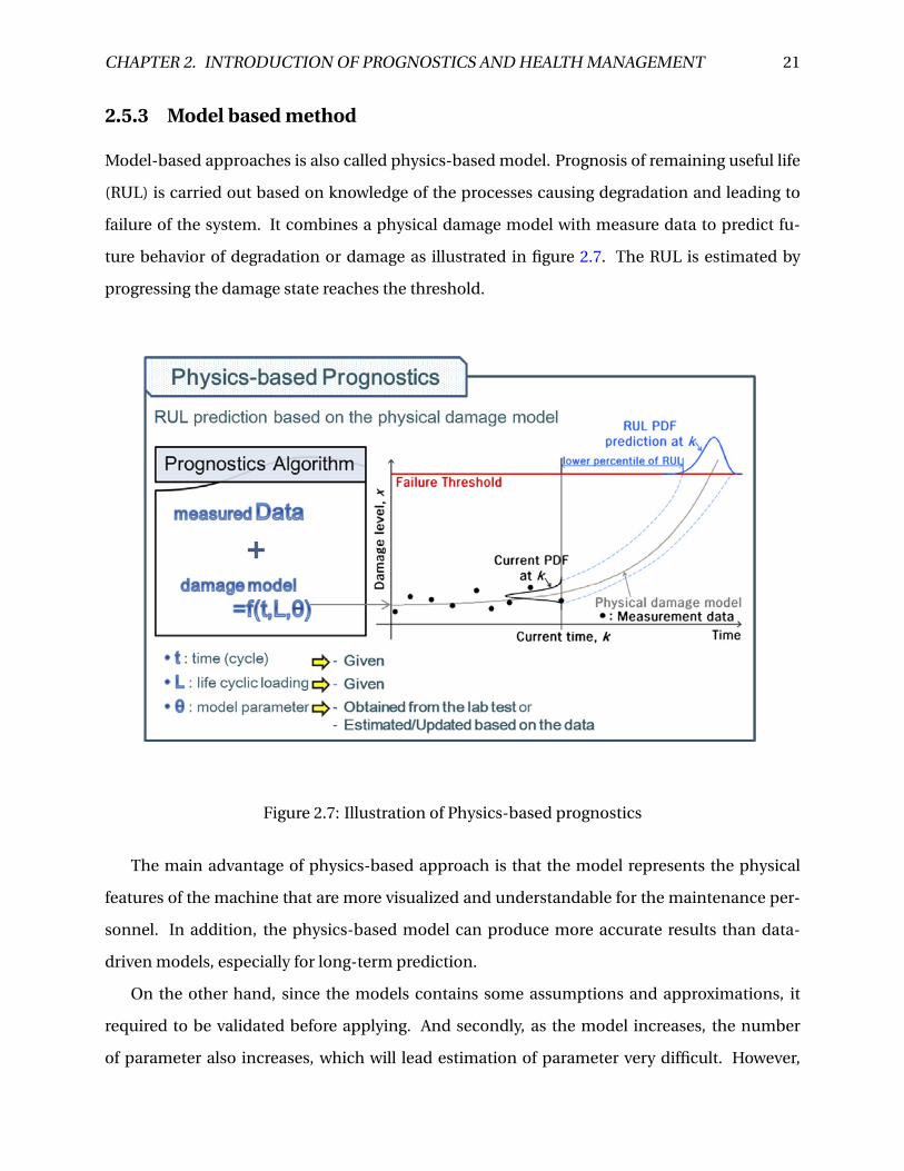
Model-based approaches is also called physics-based model. Prognosis of remaining useful life
(RUL) is carried out based on knowledge of the processes causing degradation and leading to
failure of the system. It combines a physical damage model with measure data to predict fu-
ture behavior of degradation or damage as illustrated in figure 2.7. The RUL is estimated by
progressing the damage state reaches the threshold.
Figure 2.7: Illustration of Physics-based prognostics
The main advantage of physics-based approach is that the model represents the physical
features of the machine that are more visualized and understandable for the maintenance per-
sonnel. In addition, the physics-based model can produce more accurate results than data-
driven models, especially for long-term prediction.
On the other hand, since the models contains some assumptions and approximations, it
required to be validated before applying. And secondly, as the model increases, the number
of parameter also increases, which will lead estimation of parameter very difficult. However,

CHAPTER 2. INTRODUCTION OF PROGNOSTICS AND HEALTH MANAGEMENT 22
parameter identification and estimation is the most important issue because the behavior of a
physical model depends on the model parameter estimation. Thirdly, sometimes the system is
so complex that a mathematical model can not be developed from the first principles. Finally,
due to the variate principles, different components should use different models. The process of
building models requires the personnel to have a very deep understanding of the system and it
is also very time consuming and costly.
Chapter 3
Proposed hybrid model for degradation
prognostics
In last chapter both of model-based and data-driven prognostics methods has been discussed
and compared. Unlike model-based prognostic method, data-driven prognostic approaches are
much more practicable to implement for industries because data-driven methods are easy to
understand and mostly there are a big amount of monitoring data existing. Within data-driven
methods, artificial neural networks (ANNs) and Stochastic process based models are relatively
new in applications in the reliability field and have not yet been effectively applied in remaining
asset lifetime prediction problems. These models are promising to demonstrate both linear and
nonlinear relationships between covariate data and actual asset health. In this chapter these
two methods will be used to deal with the degradation prognostics.
Degradation or deterioration problem is a common issue either for machinery or electron-
ics. Currently, the industry common strategy for degradation is using model-based diagnostic
method to send alarm if something goes wrong, however, the need to maintain high availabil-
ity of the system is necessary, which means maintenance planning in advance is prerequisite.
Therefore the prognostic ability becomes more important and imperative.
23

CHAPTER 3. PROPOSED HYBRID MODEL FOR DEGRADATION PROGNOSTICS 24
3.1 Propose a hybrid model
For machinery, many researches has been done on degradation relevant issues. The conclusion
is the Gamma process is the most suitable model for monotonic degradation issues, such as cor-
rosion, erosion, crack propagation, etc. Gamma process is a suitable method for predicting the
trend of degradation with stochastic property. Nevertheless, the assumption always made for
gamma process is that the degradation status is directly observed. In fact the indicator some-
times is not observable. For example subsea equipments are located on the seabed and difficult
for retrieval and inspection. It is difficult and time-consuming and also very costly. The prob-
lem of degradation indicator selection and extraction has not yet been studied much so far. This
paper is going to discover the method for solving the gamma process application limitation.
As the condition monitoring technology is developing fast and being applied in various in-
dustries, it becomes easier for the degradation visualization. The degradation level is not di-
rectly detected, but it is possible to monitor the relevant covariates that can be fused into a
parameter that indicates current status of the monitored system or component. For example
DWS team introduces that the tire deflation is detected not directly by the air pressure, instead,
Dunlop Tech monitors the wheel speed to indicate the deflation.
The relationship between the degradation indicator and its relevant covariates can be ei-
ther linear or non-linear, and it is normally derived from the first principles. Ideally the trend
of degradation indicator should be monotonic due to the property of the degradation, but in
reality, the results of the degradation parameter will always varies, with a lot of noise.
The non-monotone degradation parameter calculated from the monitoring data, needs to
be processed by techniques such as filtering and smoothing. When data processing is done, the
relationship between the history monitoring data set (measurable covariates) with these post-
processed values of degradation parameter could be built by ANNs model to replace the original
physics-orientated relation. The post-processed degradation parameter values are used as the
output of the ANNs, and the values of the measurable variables are fitted in ANNs as inputs.
The ANNs is trained with a certain amount of the history data sets. After training, if the future
measurable variables are collected and putted into the ANNs model, the degradation parameter
value can be obtained from the new output of ANNs, which infers the health condition of com-
CHAPTER 3. PROPOSED HYBRID MODEL FOR DEGRADATION PROGNOSTICS 25
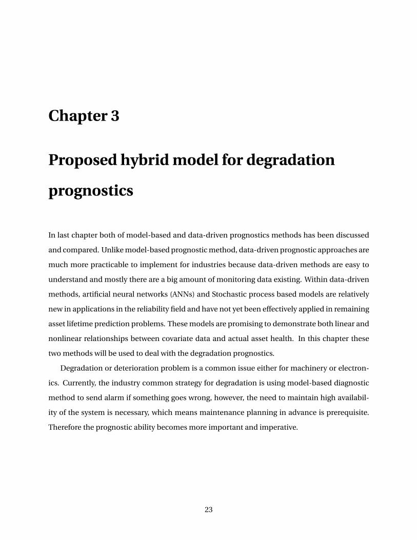
ponents or subsystems. The new output sets are the target values that is assumed as a gamma
process and used for prognostics. The technical road map of this method is shown in the figure
3.1:
Figure 3.1: The procedure of proposed method for degradation problem
In a word, a hybrid model is proposed with Artificial Neural Network for degradation state
visualization and Gamma process for degradation prognostics. And in the following content,
the theory of Artificial Neural Networks and Gamma process will be discussed in detail.
3.2 Artificial Neural Network
As described in previous chapter, artificial neural network is a flexible model that can be used
for nonlinear modeling. ANNs model relationships between input and output variables with a
model structure inspired by the neural structure of the human brain.
According to Heng et al. (2009), an ANN consists of a layer of input nodes, one or more lay-
ers of hidden nodes, one layer of output nodes and connecting weights. The network learns

CHAPTER 3. PROPOSED HYBRID MODEL FOR DEGRADATION PROGNOSTICS 26
the unknown function by adjusting its weights with repetitive observations of inputs and out-
puts. After the training process, the validation should be done using another sets of history data
before ANN is used for prediction.
Neural network can be classified into two major types: the static neural network and the dy-
namic neural network. Static neural networks have no feedback elements and contain no time
delays. Contrary to the static neural network, the dynamic neural network, the output depends
on the current or previous inputs, outputs or states of the networks. Moreover, dynamic network
can be divided into two subgroups: Dynamic networks with feed-forward connections, where
the output response depends both on inputs and time; dynamic networks with feedback or re-
current connections, where the output depends on the previous states and time. For example,
recurrent neural networks (RNNs), according to Boden (2001), have one or more feedback loops
and it has the ability to store the preceding states and record the characteristics of a system it
represents over time. The figure 3.2 shows an illustrative example of the general structure of a
recurrent network.
Figure 3.2: Recurrent Neural Network
Since the ANNs is not going to applied for prediction in this paper, the recurrent neural net-
works will be not discussed here. In the following the feed-forward neural network (FFNN) is
introduced.
CHAPTER 3. PROPOSED HYBRID MODEL FOR DEGRADATION PROGNOSTICS 27
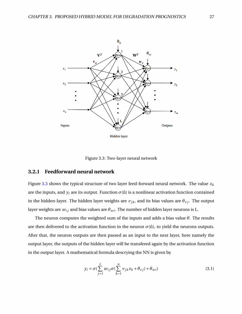
Figure 3.3: Two-layer neural network
3.2.1 Feedforward neural network
Figure 3.3 shows the typical structure of two layer feed-forward neural network. The value xk
are the inputs, and yi are its output. Function σ(u) is a nonlinear activation function contained
in the hidden-layer. The hidden layer weights are v j k , and its bias values are θv j . The output
layer weights are wi j and bias values are θwi . The number of hidden layer neurons is L.
The neuron computes the weighted sum of the inputs and adds a bias value θ. The results
are then delivered to the activation function in the neuron σ(u), to yield the neurons outputs.
After that, the neuron outputs are then passed as an input to the next layer, here namely the
output layer, the outputs of the hidden layer will be transfered again by the activation function
in the output layer. A mathematical formula descrying the NN is given by
yi =σ(L∑
j=1wi jσ(
n∑k=1
v j k xk +θv j )+θwi ) (3.1)
CHAPTER 3. PROPOSED HYBRID MODEL FOR DEGRADATION PROGNOSTICS 28
Activation functions
There is a variety of linear or non-linear activation functions in the neurons and some common
ones are step function, log-sigmoid, and tan-sigmoid functions, radial-basis, ridge polynomial,
wavelet functions. A.Poongodai and S.Bhuvaneswari (2013) claims that log-sigmoid activation
function is often used in output layer for classification problems, to limit the output to a small
range, whilst linear activation function is often used in output layer for regression problems, to
avoid limiting the output range.
Network Training
A network training procedure is to identify the optimal set of weights and bias values for each
neuron, given a set of input and output training data. The most common training approach is
the back propagation algorithm, and the procedure of network training is described here:
(1) The first step is put the training data into the network, and networks weights and bias are
randomly generated, and output can be calculated;
(2) The second step is to compare the model output yi with the target value yi from the data
set, and the sum of squared error(SSE) is computed as below:
SSE =n∑
i=1
m∑j=1
(yi − yi ) (3.2)
where n is the number of input-output samples in the training data set, m is the number of
outputs.
(3) The next step is to evaluate the error and minimize the SSE by modifying the weights
between each neuron. A common weight-tuning algorithm is the gradient algorithm based on
back-propagated error. This algorithm is given by:
Wt+1 = Wt +Fσ(VTt Xd)ET
t (3.3)
Vt+1 = Vt +GXd(σ′Tt WtEt)T (3.4)
Where t is the time index, and Et = yd−yt is the output error at time t, yd is the output value from
the training data set, yt is the model output at time t. F and G are weighting matrices selected

CHAPTER 3. PROPOSED HYBRID MODEL FOR DEGRADATION PROGNOSTICS 29
by the designer that determine the speed of convergence of the algorithm.
(4) The training process is then repeated until the error reaches a desired threshold value,
or until the required number of training iteration has been done. At that time, the network is
deemed to have done with training, and can be used for prediction.
3.2.2 NNs merits and limitations
Merits
According to Heng et al. (2009), numerous studies from various disciplines have demonstrated
the merits of ANNs:
a) It performs faster than system identification techniques in multivariate prognosis;
b) Its performance is at least as good as the best traditional statistical methods, without re-
quiring untenable distributional assumptions [33,34];
c) It is able to capture complex phenomenon without a priori knowledge.
Limitations
a) The first issue is the selection of the network architecture. There is always problems to de-
termine the number of neurons should be contained in the network, as well as the number
of layers. Lawrence has utilized the mean square errors in order to find the optimal num-
ber of neurons. Ostafe introduces a method to determine the number of hidden layers by
using pattern recognition. However, there is still no standard method. It is often a trial
and error exercise. More neurons within the network, more powerful the ability of net-
work to model more complex relationship. However, more neurons maybe lead to over fit
the data, and the generalization capability will reduce. Many issues should be considered
during network size selection.
b) Finding the optimal parameters is another problem for neural networks. As known for
more complex system the network will contain more neurons. It is extremely difficult to
find global optimum if there are many parameters, especially for back propagation.

CHAPTER 3. PROPOSED HYBRID MODEL FOR DEGRADATION PROGNOSTICS 30
c) The uncertainty caused by the noise in the data is not considered in neural network. And
there is no parameters related to the noise of data. For the noise in the data, it is com-
mon to provide the confidence bounds. Few works has been done on probabilistic neural
network in order to handle the uncertainty. Khawaja introduces a way to obtain confi-
dence bounds and also confidence distributions. The ability of handling noise of data is
still need to be improved to build confidence.
d) Lacking of transparency is also an issue that is argued by many authors. However, Bost-
wick and Burke (2001) argues that the transparency will reduce when model complexity
increase for both of traditional statistical models and ANN models. It is just that ANNs are
more capable in modeling complex phenomenon and consequently need a more complex
structure to represent the phenomenon.
e) There is no clear documentation shows how the decisions are reached in a trained neural
network, since NNs are the black box . While, Thong (2000) argues that rules can actually
be extracted from trained ANNs to explain how decisions are reached.
3.3 Stochastic Process
As discussed in chapter 2.6, the stochastic process is a very powerful method to model the
temporal uncertainty associated with the evolution of deterioration. And the common used
stochastic process are Gamma process, Wiener process and Levy process. Since most of the
degradation is monotone and random, which makes Gamma process most suitable model for
analyzing the wear and fatigue propagation, corrosion, erosion, etc. And it overcomes the prob-
lem of random coefficient regression based model. The regression based model is simple to
implement but they are lacking of temporal randomness even if they use nonlinear regression,
and also the regression based model may not be able to derive a closed-form expressions for
time to failure(TTF) distribution or residual useful life (RUL) distribution.
In the Gamma process model, the cumulative deterioration X (t ) at time t follows a gamma
distribution, with a shape function λ(t ) > 0 and a scale parameter u > 0, which is a constant
value. Since gamma process has the monotonic property, the shape function λ(t ) is required
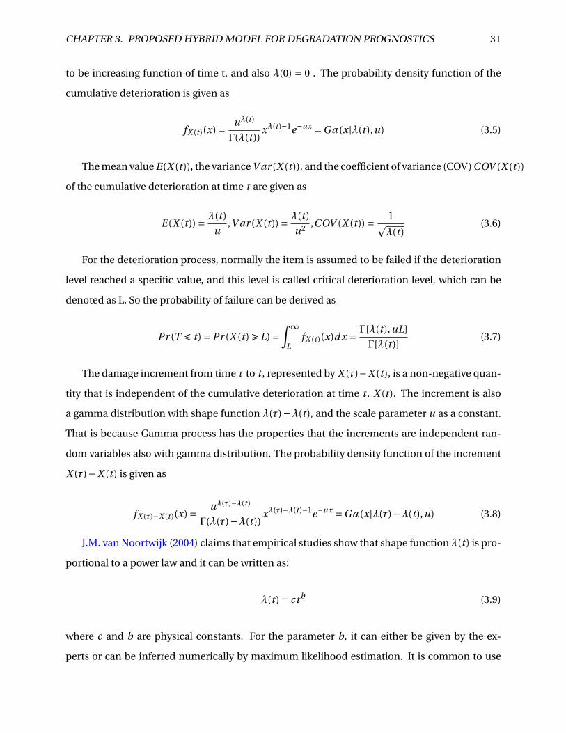
CHAPTER 3. PROPOSED HYBRID MODEL FOR DEGRADATION PROGNOSTICS 31
to be increasing function of time t, and also λ(0) = 0 . The probability density function of the
cumulative deterioration is given as
fX (t )(x) = uλ(t )
Γ(λ(t ))xλ(t )−1e−ux =Ga (x|λ(t ),u) (3.5)
The mean value E(X (t )), the variance V ar (X (t )), and the coefficient of variance (COV) COV (X (t ))
of the cumulative deterioration at time t are given as
E(X (t )) = λ(t )
u,V ar (X (t )) = λ(t )
u2,COV (X (t )) = 1p
λ(t )(3.6)
For the deterioration process, normally the item is assumed to be failed if the deterioration
level reached a specific value, and this level is called critical deterioration level, which can be
denoted as L. So the probability of failure can be derived as
Pr (T É t ) = Pr (X (t ) Ê L) =∫ ∞
LfX (t )(x)d x = Γ[λ(t ),uL]
Γ[λ(t )](3.7)
The damage increment from time τ to t , represented by X (τ)−X (t ), is a non-negative quan-
tity that is independent of the cumulative deterioration at time t , X (t ). The increment is also
a gamma distribution with shape function λ(τ)−λ(t ), and the scale parameter u as a constant.
That is because Gamma process has the properties that the increments are independent ran-
dom variables also with gamma distribution. The probability density function of the increment
X (τ)−X (t ) is given as
fX (τ)−X (t )(x) = uλ(τ)−λ(t )
Γ(λ(τ)−λ(t ))xλ(τ)−λ(t )−1e−ux =Ga (x|λ(τ)−λ(t ),u) (3.8)
J.M. van Noortwijk (2004) claims that empirical studies show that shape function λ(t ) is pro-
portional to a power law and it can be written as:
λ(t ) = ct b (3.9)
where c and b are physical constants. For the parameter b, it can either be given by the ex-
perts or can be inferred numerically by maximum likelihood estimation. It is common to use

CHAPTER 3. PROPOSED HYBRID MODEL FOR DEGRADATION PROGNOSTICS 32
expert judgment to get the value of b, for example, sometimes b equals to 1 for simplicity, which
means λ(t ) = ct . In this case, it is a stationary gamma process, where the average deterioration
increases linearly with time. According to J.M. van Noortwijk (2004), the gamma process is not
restricted to using a power law for modeling the expected deterioration over time. As a matter
of fact, any shape function λ(t ) suffices, as long as it is a non-decreasing, right continuous, and
real-valued function. So now the probability density function is
fX (t )(x) = uct b
Γ(ct b)xct b−1e−ux =Ga
(x|ct b ,u
)(3.10)
After substitute λ(t ) withct b , the mean and variance is given as
E(X (t )) = ct b
u,V ar (X (t )) = ct b
u2(3.11)
3.3.1 Parameter Estimation
The commonly used estimation methods are Probability Plotting, Least Squares, Maximum
Likelihood Estimation and Bayesian Estimation Methods. A paper on Reliawiki said the method
of maximum likelihood estimation method is, with some exceptions, considered to be the most
robust of the parameter estimation techniques. In general, for a fixed set of data and underlying
statistical model, the method of maximum likelihood selects values of the model parameters
that produce a distribution that gives the observed data the greatest probability (i.e., parame-
ters that maximize the likelihood function). Assuming we have n observations x1, x2, .., xn . The
principle of maximum likelihood assumes that the sample data set is representative of the pop-
ulation with a probability density function of f (x1, x2, .., xn ;θ) and chooses that value for θ (un-
known parameter) that most likely caused the observed data to occur.
The maximum likelihood function can be setting up by using the independent increments
di = X (ti )−X (ti−1) in interval (ti−1, ti ), di is a product of independent gamma densities:
L(d1,d2, ...,dn |c,u) =n∏
i=1fX (ti )−X (ti−1)(di )
=n∏
i=1
uc(tbi −tb
i−1)
Γ[c(t bi −t b
i−1)]d
c(t bi −t b
i−1)
i e−udi
(3.12)
CHAPTER 3. PROPOSED HYBRID MODEL FOR DEGRADATION PROGNOSTICS 33
We know the cumulative amounts of deterioration at last inspection time tn are measured as
xn , so the Expected value E(X (tn)) = xn . And since E(x(tn)) = ct bn
u , the estimated value of scale
parameter can be derived as
u = c t bn
xn(3.13)
3.3.2 Estimation of RUL
After estimating parameters of Gamma distribution function, the reliability function of time to
failure could be deduced. For a single item, R(t ) is the probability of the deterioration level at
time t smaller than the critical threshold L, and it can be derived as
R(t ) = Pr (T Ê t )
= Pr (X É L)
= Pr (X t −X0 É L)
= ∫ L0 Ga (v |ct ,u)d v
(3.14)
Similarly, the conditional reliability function, given that at time the item is still functioning
at time t j can be given as
R(t |T > t j ) = Pr (T Ê t |T > t j )
= Pr (X t É L|T > t j )
= Pr (X t −X0 É L|X t j −X0 < L)
=∫ L
0 Ga(v |ct ,u)d v∫ L0 Ga(v |ct j ,u)du
(3.15)
Finally, the residual useful life distribution function RRU L(h) at time t j can be derived as
RRU L(t j )(h) = Pr (RU L(t j ) > h)
= Pr (X t j+h < L|X t j < L, X t j = xt j )
= Pr (X t j+h −X t j É L−xt j |X t j < L)
=∫ L−xt j
0 Ga(v |ch,u)d v∫ L0 Ga(v |αt j ,β)d v
(3.16)

CHAPTER 3. PROPOSED HYBRID MODEL FOR DEGRADATION PROGNOSTICS 34
3.3.3 Merits and Limitations
Merits
a) Gamma process is a stochastic process and it can account for the population variability
and temporal variability associated with a degradation process.
b) Gamma process has a straightforward mathematic calculations and it is easy to under-
stand.
Limitations
a) Gamma process is only suitable for modeling the wear and fatigue issues, with a strictly
monotonic process. Or this can also be the advantage of Gamma process in terms of
monotonic process.
b) The degradation state should be observed directly. This can be solved by this hybrid
model.

Chapter 4
Hybrid model application on subsea valves
Subsea industry is growing very fast in 21st century, since the easy fields in the world have al-
ready been explored, and the left oil and gas reservoir is far from shore and deep under water.
However, the maintenance for subsea equipments are different from topside facilities, much
longer time needed for retrieval of failed equipments and replacement of new one. Even though
the condition monitoring has applied for many subsea equipments, the utilization ability of
monitoring data and prognostics algorithms has not been deeply explored. In this paper, a sub-
sea choke valve will be studied as a case, and the relevant prognostics issues are going to be
discussed in this chapter.
4.1 Subsea choke valves introduction
As the choke valves used on topside, the subsea choke valves regulates the main flow from its
corresponding wells into a common manifold. There are many suppliers of subsea chokes,
namely, FMC Technologies, Master Flo, Cameron, etc. Different suppliers offers different types
of subsea choke valves. While, according to Cameron website Cameron (2009), subsea chokes
are typically used to:
• Start up and shut in subsea wells
• Balance pressures from different wells to a common manifold
• Reduce flow line pressures and costs
35
CHAPTER 4. HYBRID MODEL APPLICATION ON SUBSEA VALVES 36
• Protect against reservoir collapse during startup
• Control flow rates to extend production life
• Protect subsea gate valves from high-pressure drops during startup and shutdown
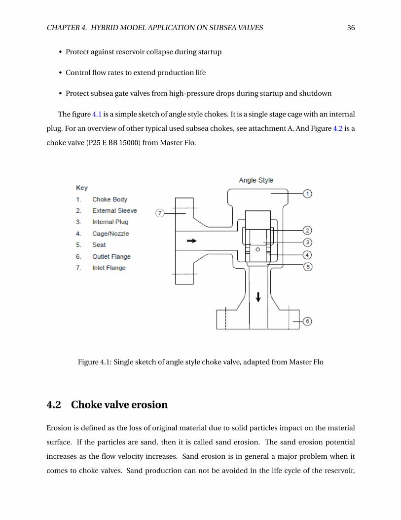
The figure 4.1 is a simple sketch of angle style chokes. It is a single stage cage with an internal
plug. For an overview of other typical used subsea chokes, see attachment A. And Figure 4.2 is a
choke valve (P25 E BB 15000) from Master Flo.
Figure 4.1: Single sketch of angle style choke valve, adapted from Master Flo
4.2 Choke valve erosion
Erosion is defined as the loss of original material due to solid particles impact on the material
surface. If the particles are sand, then it is called sand erosion. The sand erosion potential
increases as the flow velocity increases. Sand erosion is in general a major problem when it
comes to choke valves. Sand production can not be avoided in the life cycle of the reservoir,

CHAPTER 4. HYBRID MODEL APPLICATION ON SUBSEA VALVES 37
Figure 4.2: Choke valve P25 E BB 15000, adapted from Master Flo
especially in the late life phase when the pressure starts decreasing dramatically. For economic
purpose downstream pressure at the choke valve is decreased to enhance the production rate,
however at the same time more sand will pass through the choke valve and therefore increases
the erosion rate of choke valve.
Many researches have been done so far within the choke erosion. Peri and Rogers (2007)
has introduced how CFD can be used for modeling the erosion of choke valves. With the help
of experiments or computational fluid dynamic modeling, many models for assessing the sand
erosion rate are developed. Veritas (2007) has made a outline of most of the methods for piping
systems. Sæther (2010) introduces some models for calculating choke valves erosion rate and
CHAPTER 4. HYBRID MODEL APPLICATION ON SUBSEA VALVES 38
also claims that Cv of valves is the best indicator on choke valve erosion.
Flow coefficient(Cv ) of a device is a relative measure of its efficiency at allowing fluid flow. It
describes the relationship between the pressure drop across an orifice, valve or other assembly
and the corresponding flow rate. Therefore, the flow coefficient (Cv ) is an important indicator
of choke performance, and the difference between the actual and theoretical flow coefficient,
δCv =C acv −C th
v , could be a good indicator of the valve erosion level.
4.3 Hybrid model for choke RUL estimation
In terms of choke erosion, directly observing the erosion level of the subsea choke valves is an
unpractical issue, since they are located several hundred meters under the seawater, sometime
even several thousand meters. Even for the retrievable subsea choke valve, it is also undesired
from the economic point of view. From last section, the δCv is considered to be a good choke
valve degradation state indicator. If the value of indicator is obtained, Gamma process can be
a practicable model for choke erosion prediction. In the next two sections the procedure of the
application of hybrid model will be introduced in detail.
Before discussing the hybrid model for choke erosion, the issue of data set used in this paper
is discussed here. Since the choke valves have been used for many decades in oil and gas in-
dustry and condition monitoring technologies are also developed many years ago, there should
exist many historical records of chokes operational and environmental condition data. Unfortu-
nately the data normally is kept by the operation companies as their secret database. So in this
paper, the data used is generated artificially from Matlab and it is just used for model demon-
stration. The data set for 10 similar choke valves are listed in the appendix. The purpose is to
show how the hybrid model is used for choke valve erosion prognostics and RUL calculation.
4.4 Visualization of the erosion indicator
4.4.1 Calculating δCv
The theoretical flow coefficient C thv is always provided by the valve supplier, and is dependent
on the valve type and valve opening (Stem travel shown in figure 4.3 ). An example is shown in
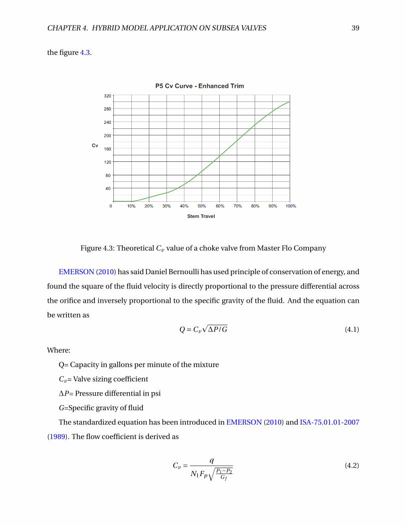
CHAPTER 4. HYBRID MODEL APPLICATION ON SUBSEA VALVES 39
the figure 4.3.
Figure 4.3: Theoretical Cv value of a choke valve from Master Flo Company
EMERSON (2010) has said Daniel Bernoulli has used principle of conservation of energy, and
found the square of the fluid velocity is directly proportional to the pressure differential across
the orifice and inversely proportional to the specific gravity of the fluid. And the equation can
be written as
Q =Cv
p∆P/G (4.1)
Where:
Q= Capacity in gallons per minute of the mixture
Cv = Valve sizing coefficient
∆P= Pressure differential in psi
G=Specific gravity of fluid
The standardized equation has been introduced in EMERSON (2010) and ISA-75.01.01-2007
(1989). The flow coefficient is derived as
Cv = q
N1Fp
√P1−P2
G f
(4.2)

CHAPTER 4. HYBRID MODEL APPLICATION ON SUBSEA VALVES 40
Where q = qg + qw + qo , is the total volumetric flow rate of the mixture (kg /h). N1 = 0.865,
the value of N is shown in the Appendix B B.8. Fp is the so-called piping geometry factor and
P1 −P2 is the pressure drop across the valve (bar), G f is specific gravity of the mixture. And the
specific gravity of the mixture can be calculated as
G f =
(fg
ρg∗J 2 + fwρw
+ foρo
)−1
ρw(4.3)
Theoretically the relationship between the flow coefficient with other basic value type vari-
ables, such as pressure, temperature, and flow rate is built. Practically, the temperature, pres-
sure, flow rate and the opening angle can be collected by high-tech sensors. With the devel-
opment of the sensor technologies, it boosts the speed of implementing condition monitoring.
The sensors for metering the temperature, pressure, and flow rate have already been used for
oil and gas industry for many decades. Therefore on basis of on-line monitoring, the model
based method for indicator visualization is to calculate the difference between the actual and
theoretical flow coefficient, δCv , can be derived as
δCv =C acv −C th
v
= q
N1Fp
√(P1−P2)
(fg
ρg ∗J2 + fwρw
+ foρo
)−1
/ρw
−C thv
(4.4)
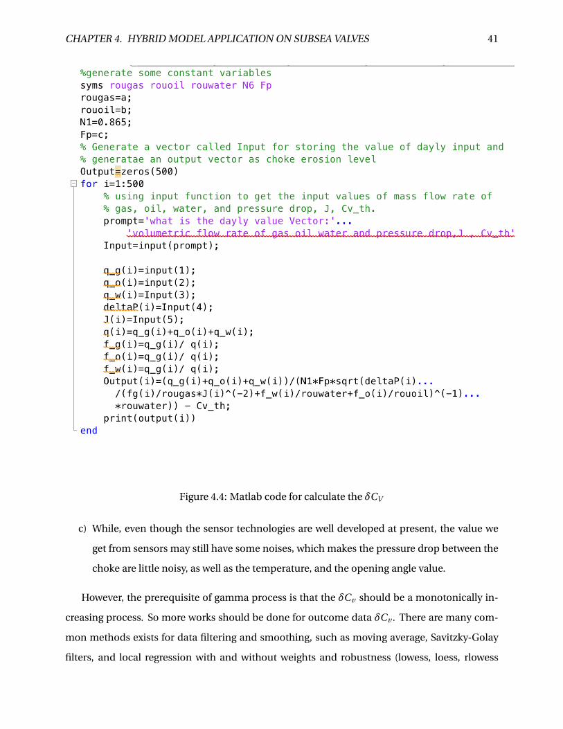
This calculation of δCv can be carried out by Matlab directly, and the simple code is shown
in figure 4.4 for demonstration.
4.4.2 Filtering of δCv
Fitting in the actual everyday average value of the six on-line monitoring variables, the trend of
outcome should be slightly increasing from the beginning, but it varies quite much, not always
a monotonic increment. The main reasons are listed below:
a) The big sharp variance is due to the short valve opening variations;
b) The value of everyday flow rate of oil, gas, and water is not precise enough;
CHAPTER 4. HYBRID MODEL APPLICATION ON SUBSEA VALVES 41
Figure 4.4: Matlab code for calculate the δCV
c) While, even though the sensor technologies are well developed at present, the value we
get from sensors may still have some noises, which makes the pressure drop between the
choke are little noisy, as well as the temperature, and the opening angle value.
However, the prerequisite of gamma process is that the δCv should be a monotonically in-
creasing process. So more works should be done for outcome data δCv . There are many com-
mon methods exists for data filtering and smoothing, such as moving average, Savitzky-Golay
filters, and local regression with and without weights and robustness (lowess, loess, rlowess
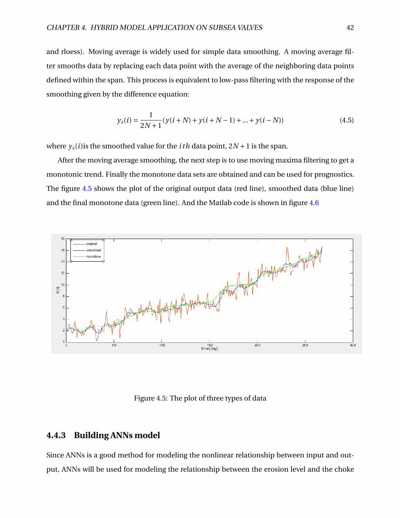
CHAPTER 4. HYBRID MODEL APPLICATION ON SUBSEA VALVES 42
and rloess). Moving average is widely used for simple data smoothing. A moving average fil-
ter smooths data by replacing each data point with the average of the neighboring data points
defined within the span. This process is equivalent to low-pass filtering with the response of the
smoothing given by the difference equation:
ys(i ) = 1
2N +1(y(i +N )+ y(i +N −1)+ ...+ y(i −N )) (4.5)
where ys(i )is the smoothed value for the i th data point, 2N +1 is the span.
After the moving average smoothing, the next step is to use moving maxima filtering to get a
monotonic trend. Finally the monotone data sets are obtained and can be used for prognostics.
The figure 4.5 shows the plot of the original output data (red line), smoothed data (blue line)
and the final monotone data (green line). And the Matlab code is shown in figure 4.6
Figure 4.5: The plot of three types of data
4.4.3 Building ANNs model
Since ANNs is a good method for modeling the nonlinear relationship between input and out-
put, ANNs will be used for modeling the relationship between the erosion level and the choke
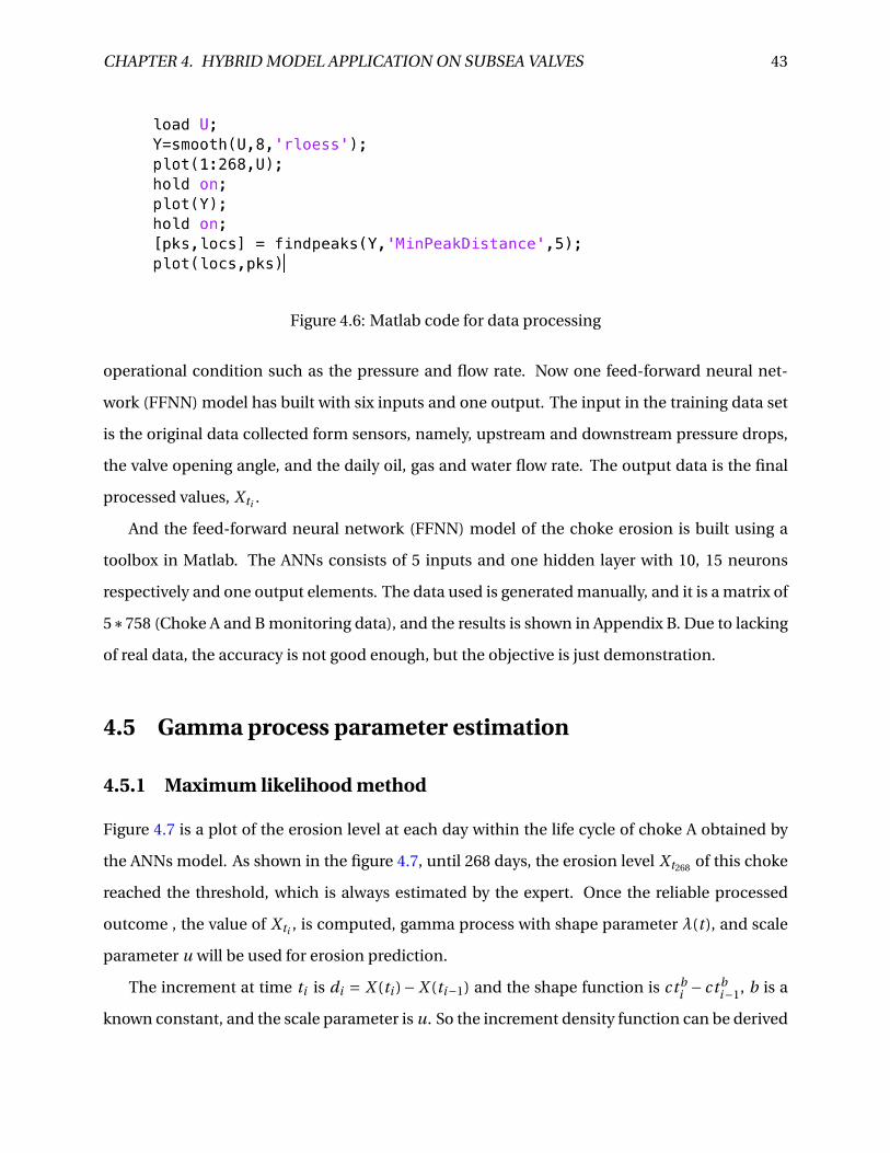
CHAPTER 4. HYBRID MODEL APPLICATION ON SUBSEA VALVES 43
Figure 4.6: Matlab code for data processing
operational condition such as the pressure and flow rate. Now one feed-forward neural net-
work (FFNN) model has built with six inputs and one output. The input in the training data set
is the original data collected form sensors, namely, upstream and downstream pressure drops,
the valve opening angle, and the daily oil, gas and water flow rate. The output data is the final
processed values, X ti .
And the feed-forward neural network (FFNN) model of the choke erosion is built using a
toolbox in Matlab. The ANNs consists of 5 inputs and one hidden layer with 10, 15 neurons
respectively and one output elements. The data used is generated manually, and it is a matrix of
5∗758 (Choke A and B monitoring data), and the results is shown in Appendix B. Due to lacking
of real data, the accuracy is not good enough, but the objective is just demonstration.
4.5 Gamma process parameter estimation
4.5.1 Maximum likelihood method
Figure 4.7 is a plot of the erosion level at each day within the life cycle of choke A obtained by
the ANNs model. As shown in the figure 4.7, until 268 days, the erosion level X t268 of this choke
reached the threshold, which is always estimated by the expert. Once the reliable processed
outcome , the value of X ti , is computed, gamma process with shape parameter λ(t ), and scale
parameter u will be used for erosion prediction.
The increment at time ti is di = X (ti )− X (ti−1) and the shape function is ct bi − ct b
i−1, b is a
known constant, and the scale parameter is u. So the increment density function can be derived
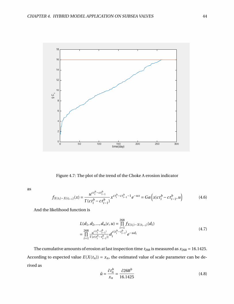
CHAPTER 4. HYBRID MODEL APPLICATION ON SUBSEA VALVES 44
Figure 4.7: The plot of the trend of the Choke A erosion indicator
as
fX (ti )−X (ti−1)(x) = uct bi −ct b
i−1
Γ(ct bi − ct b
i−1)xct b
i −ct bi−1−1e−ux =Ga
(x|ct b
i − ct bi−1,u
)(4.6)
And the likelihood function is
L(d1,d2, ...,dn |c,u) =268∏i=1
fX (ti )−X (ti−1)(di )
=268∏i=1
uc(tbi −tb
i−1)
Γ[c(t bi −t b
i−1)]d
c(t bi −t b
i−1)
i e−udi
(4.7)
The cumulative amounts of erosion at last inspection time t268 is measured as x268 = 16.1425.
According to expected value E(X (tn)) = xn , the estimated value of scale parameter can be de-
rived as
u = c t bn
xn= c268b
16.1425(4.8)
CHAPTER 4. HYBRID MODEL APPLICATION ON SUBSEA VALVES 45
Taking logarithm of the likelihood function, the log-likelihood function is
∂∂c l og L(d1,d2, ...,dn |c,u)
=n∑
i=1
∂∂c
{c[t b
i − t bi−1]log
(ct b
nxn
)− l ogΓ(c[t b
i − t bi−1])+ (
c[t bi − t b
i−1]−1)
logδi − ct bn
xnδi
}=
n∑i=1
{[t b
i − t bi−1]
[log
(ct b
nxn
)+1−ψ(c[t b
i − t bi−1])+ logδi
]− t b
nxnδi
}= t b
n log(
ct bn
xn
)+
n∑i=1
[t bi − t b
i−1]{logδi −ψ(c[t b
i − t bi−1])
}= 0
(4.9)
Where the function ψ(a) is the derivative of the logarithm of the gamma function:
ψ(a) = Γ′(a)
Γ(a)= ∂logΓ(a)
∂a(4.10)
for a > 0. Summarizing the maximum likelihood estimation, we can get
u = c268b
16.1425,
268∑i=1
[t bi − t b
i−1]{ψ(c[t b
i − t bi−1])− logδi
}= 268blog
(c268b
16.1425
)(4.11)
The parameter b is assumed to be 1, and the other two parameters c and β are estimated
by Matlab, and the code is shown below in figure 4.8. The result from the maximum likelihood
estimation is listed as formula 4.12 and the figure of estimated expected erosion level is shown in
figure 4.9, and some other figures with different b values are shown in the Appendix. In addition,
for Choke B, the results are shown in the Appendix.
c = 0.8487, u = 14.0902 (4.12)
As shown in figure 4.9, the red line is actual δCv and the blue line is the plot of estimated
value. The erosion level is overestimated when t < 160, while it is underestimated by the ex-
pected value from the gamma proces when t > 160. The same happens with the other b values
(b 6= 1), even though they do not represent linear increments. The solution for this problem is to
use Bayesian method for updating estimate parameters to reach a more precise estimation.
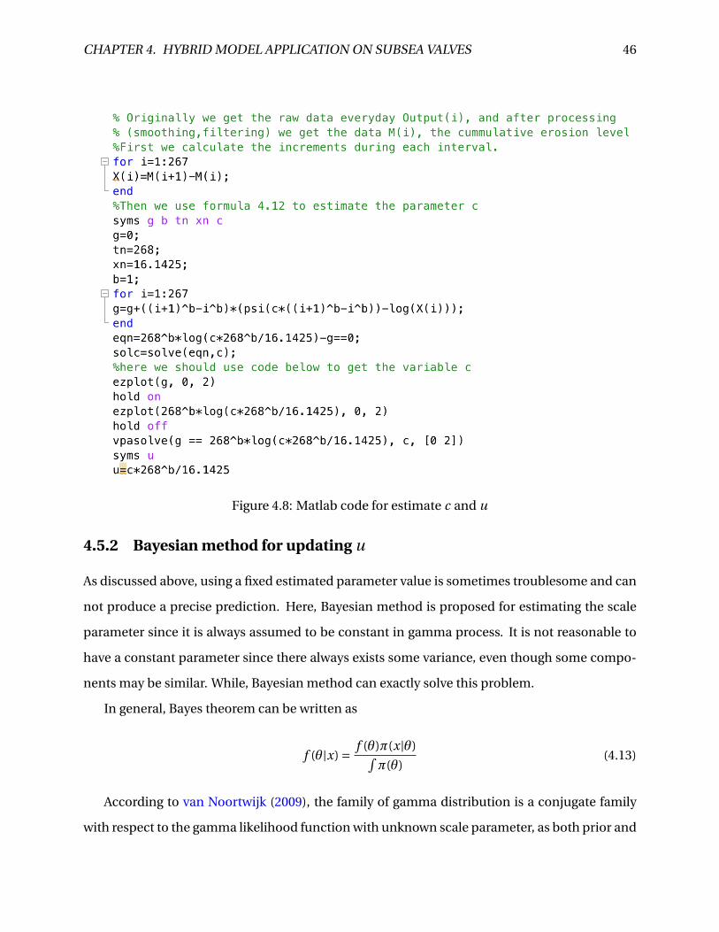
CHAPTER 4. HYBRID MODEL APPLICATION ON SUBSEA VALVES 46
Figure 4.8: Matlab code for estimate c and u
4.5.2 Bayesian method for updating u
As discussed above, using a fixed estimated parameter value is sometimes troublesome and can
not produce a precise prediction. Here, Bayesian method is proposed for estimating the scale
parameter since it is always assumed to be constant in gamma process. It is not reasonable to
have a constant parameter since there always exists some variance, even though some compo-
nents may be similar. While, Bayesian method can exactly solve this problem.
In general, Bayes theorem can be written as
f (θ|x) = f (θ)π(x|θ)∫π(θ)
(4.13)
According to van Noortwijk (2009), the family of gamma distribution is a conjugate family
with respect to the gamma likelihood function with unknown scale parameter, as both prior and

CHAPTER 4. HYBRID MODEL APPLICATION ON SUBSEA VALVES 47
Figure 4.9: Estimated expected δCv when b=1
posterior distribution belong to the family of gamma distributions. Therefore, scale parameter
u is assumed to be a gamma distribution with shape parameter α and scale parameter β. The
prior distribution of scale parameter u can be written as
f (u|α,β) = βα
Γ(α)uα−1exp(−uβ) (4.14)
The parameters α and β is either from expert judgment, or derived from parameter estima-
tion. Here assuming that for the historical data of similar valves, maximum likelihood has been
used for estimating c and u, and then the expected value of u and variance of u can be easily
derived. According to the property of gamma distribution, E(u) = αβ
and V (u) = αβ2 , the value of
α and β can be calculated.

CHAPTER 4. HYBRID MODEL APPLICATION ON SUBSEA VALVES 48
And the posterior distribution can be derived as
f (u|d1,d2, ...,dn) = f (u|α,β)L(d1,d2, ...,dn)
= βα
Γ(α) uα−1exp(−uβ)n∏
i=1
uc(tbi −tb
i−1)
Γ[c(t bi −t b
i−1)]d
c(t bi −t b
i−1)
i e−udi
=Ga(u|α+ ct bn ,β+xn)×
(1
β+xn
)α+ct bn βαΓ(α+ct b
n )Γ(α)
n∏i=1
dic(tb
i −tbi−1)
Γ(c(t bi −t b
i−1))
∝Ga(u|α+ ct bn ,β+xn)
(4.15)
Where c is an known variable, which is estimated by maximum likelihood function. As
shown in the formula 4.15, the posterior distribution of u is also a gamma distribution with
shape parameter α+ ct bn and scale parameter β+xn .
As discussed in last section, the parameter b is assumed to be 1, and other parameters c and
u are estimated by maximum likelihood method. For parameter u, the expected value is 14, and
the variance is 9. To make the prediction more precise, the Bayesian method will be applied for
updating parameter u. so the prior distribution of u is Ga(u|α= 1.6,β= 21.7), once a new Xi is
collected, then derive the posterior distribution. The Beyes esimate is given by the mean in this
distribution of u.
u = α+ cti
β+xi= 21.7+ cti
1.6+xi(4.16)
After applying Bayes method, the prediction is shown in the figure 4.10. From the plot, it
shows that as more data collected for the choke A, more precise the prediction will be.
4.6 Residual useful life Prediction
For choke A, by setting the erosion threshold, L = 16, and b = 1,c = 0.85,u = 14 the cumulative
lifetime distribution can be obtained as
F (t ) = Pr (T É t ) = Pr (X Ê L) =∫ ∞
16
140.85t
Γ(0.85t )x0.85t−1e−14xd x = Γ(0.85t ,14∗16)
Γ(0.85t )(4.17)
Plot the F (t ) in Matlab, the plot is with some error, since the data is generated randomly.
And also because the estimation of parameters is at time t = 0 without Bayesian method is not

CHAPTER 4. HYBRID MODEL APPLICATION ON SUBSEA VALVES 49
Figure 4.10: Estimated expected δCv when b=1 with Bayesian method
accurate. However when t = 100, with Bayesian estimation of scale parameter, u = 2.97, and the
plot of F (t |X t100 ) is shown below in figure 4.11 the cumulative distribution function of the RUL
is derives as
F (t |X100) = Pr (T É t |X100 = 7.23)
= Pr (X t Ê L)
= ∫ ∞16
2.970.85t
Γ(0.85t ) x0.85t−1e−2.97xd x
= Γ(0.85t ,2.97∗16)Γ(0.85t )
(4.18)
The residual useful life distribution at time t = 100d ay s is calculated as equation4.19 and
the plot of the cumulative distribution of RUL at t = 100 is shown in figure 4.12
FRU L(t100)(h) = Pr (RU L(t100) < h)
= Pr (X t100+h > L|X t100 < L, X t100 = 7.23)
= Pr (X t100+h −X t100 Ê L−xt100 |X t100 < L)
=∫ ∞
L−xt jGa
(v |ch,
α+ct jβ+xt j
)d v
∫ L0 Ga
(v |ct j ,
α+ct jβ+xt j
)d v
(4.19)
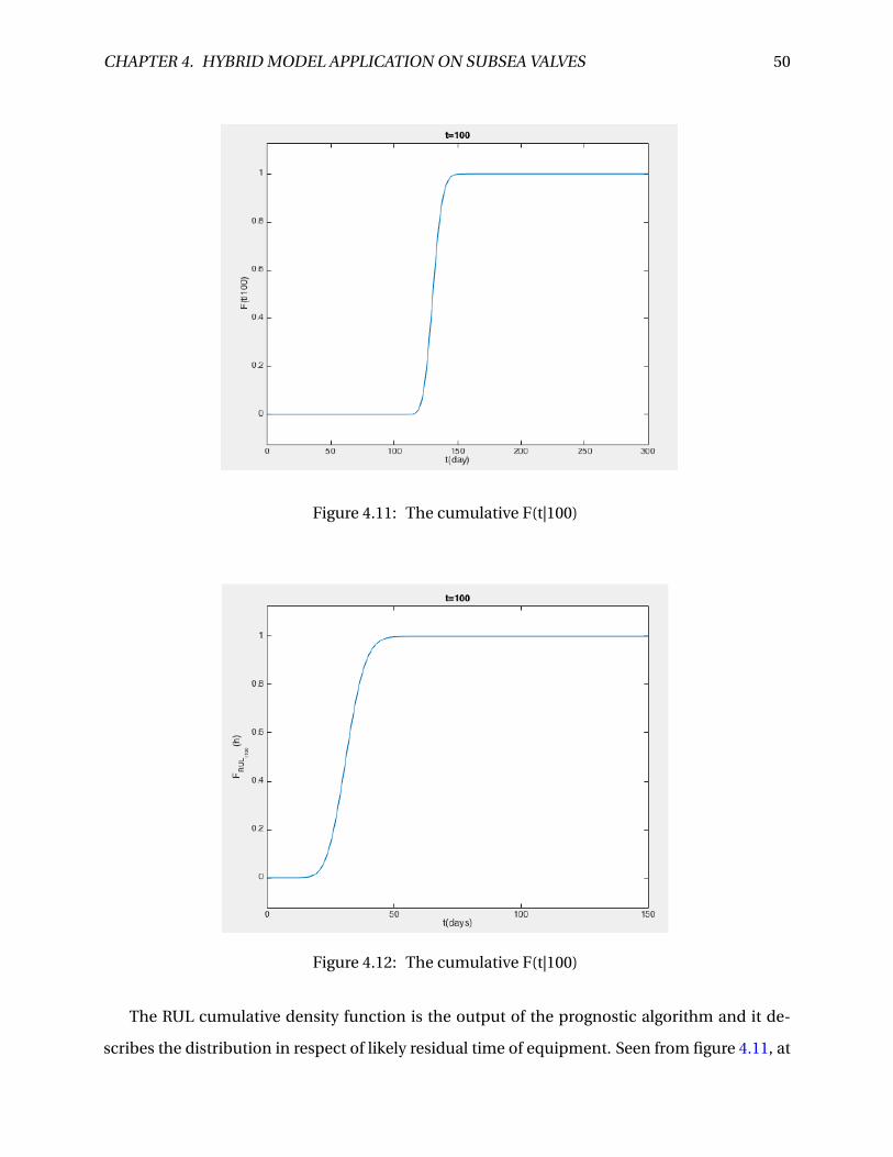
CHAPTER 4. HYBRID MODEL APPLICATION ON SUBSEA VALVES 50
Figure 4.11: The cumulative F(t|100)
Figure 4.12: The cumulative F(t|100)
The RUL cumulative density function is the output of the prognostic algorithm and it de-
scribes the distribution in respect of likely residual time of equipment. Seen from figure 4.11, at

CHAPTER 4. HYBRID MODEL APPLICATION ON SUBSEA VALVES 51
time t = 100d ay s the residual life estimation is generated. If the acceptable probability of fail-
ure is 0.1, which defines the acceptable risk level, the latest time when the maintenance must
to be carried out is about 30 days in the future. Considering other aspects such as the time
length needed for maintenance (MTTR), the availability of spare parts together with the RUL,
the optimal maintenance schedule will be decided.
Chapter 5
Summary and recommendations for further
work
5.1 Summary and conclusions
The thesis has presented the main content of prognostics and health management and its pro-
cedure. It summarized the relevant theory and techniques within each steps, namely, data ac-
quisition and processing, and diagnostics and prognostics which is the foundation of decision
making. In addition, a systematic and comprehensive review of different methods and mod-
els for diagnostics and prognostics has been presented, such as the statistical control method
for diagnostics and the the conventional reliability method, artificial intelligence method, and
stochastic methods and model based method for prognostics.
After the review, the problem of degradation prognostics is discussed. Various research has
done on degradation and gamma process is approved to be a well known stochastic method for
solving degradation problems. Whilst the problem of the unobservable degradation indicator
has not been deeply studied. In this paper, a proposed hybrid model is introduced and devel-
oped to deal with the limitation of applying Gamma process into the degradation prognostics.
The hybrid model first trains a ANNs model to use the indirect monitored variables to obtain a
monotonically increasing degradation indicator, and the data processing tasks need to be done
before the ANNs training. And the next step is to apply Gamma process to the degradation
prognostics and calculate the residual useful life. The gamma process parameter estimation
52
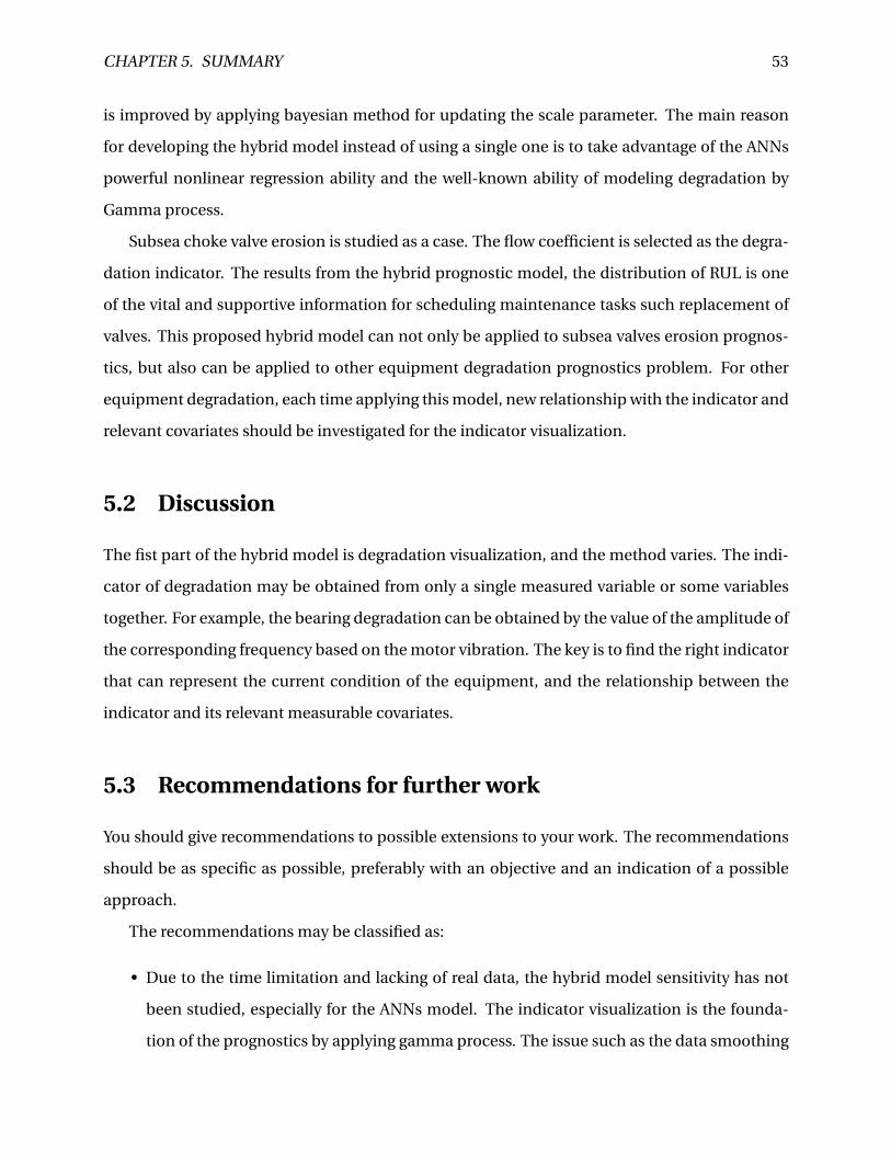
CHAPTER 5. SUMMARY 53
is improved by applying bayesian method for updating the scale parameter. The main reason
for developing the hybrid model instead of using a single one is to take advantage of the ANNs
powerful nonlinear regression ability and the well-known ability of modeling degradation by
Gamma process.
Subsea choke valve erosion is studied as a case. The flow coefficient is selected as the degra-
dation indicator. The results from the hybrid prognostic model, the distribution of RUL is one
of the vital and supportive information for scheduling maintenance tasks such replacement of
valves. This proposed hybrid model can not only be applied to subsea valves erosion prognos-
tics, but also can be applied to other equipment degradation prognostics problem. For other
equipment degradation, each time applying this model, new relationship with the indicator and
relevant covariates should be investigated for the indicator visualization.
5.2 Discussion
The fist part of the hybrid model is degradation visualization, and the method varies. The indi-
cator of degradation may be obtained from only a single measured variable or some variables
together. For example, the bearing degradation can be obtained by the value of the amplitude of
the corresponding frequency based on the motor vibration. The key is to find the right indicator
that can represent the current condition of the equipment, and the relationship between the
indicator and its relevant measurable covariates.
5.3 Recommendations for further work
You should give recommendations to possible extensions to your work. The recommendations
should be as specific as possible, preferably with an objective and an indication of a possible
approach.
The recommendations may be classified as:
• Due to the time limitation and lacking of real data, the hybrid model sensitivity has not
been studied, especially for the ANNs model. The indicator visualization is the founda-
tion of the prognostics by applying gamma process. The issue such as the data smoothing

CHAPTER 5. SUMMARY 54
method, the input numbers of ANNs model should be studied further in the future re-
search.
• Electrical equipments are more commonly used in industries, for example, Subsea in-
dustry is focus on developing all electrical control systems. However, in this paper more
focus is put on machinery, therefore, the models for electronics deterioration prognostics
should be paid more attention.
• The subsystems or the components health condition assessment and their fault prognos-
tics are the main focus at present, however, it is also very important to get the health status
at the the system level.

Appendix A
Acronyms
PM Preventive maintenance
CM Corrective maintenance
CBM Condition-based maintenance
PHM Prognostics and health management
CM Condition monitoring
SPC Statistical process control
PCA Principal component analysis
PLS Partial least squares
MTBF Mean time between failure
TTF Time to failure
AI Artificail intelligent
SVM Support vector machines
ANNs Artificial neural networks
RNN Recurrent neural network
55

APPENDIX A. ACRONYMS 56
FFNN Feed-forward neural network
RUL Residual useful life
Var Variance
COV Coefficient of variance
MLE Maximum likelihood estimation
Appendix B
B.1 ANNs
Figure B.1: The simulation results of ANNs fitting when there are 10 neurons in hidden layer
57

APPENDIX B. 58
Figure B.2: The simulation results of ANNs fitting when there are 15 neurons in hidden layer
B.2 Choke A
For choke A, using maximum likelihood estimation for parameter c and u, when assuming b =0.5 and the results is c = 23.15, u = 23.47; when assuming b = 1.5, the estimated parameter c =2.83, u = 0.8. The following two figures ?? and B.5 are the plots of the estimated expected δCv
B.3 Choke B
For choke B, the plot of the degradation trend that obtained from the ANNs model is shown in
figureB.6.
The maximum likelihood estimation code is shown below in figure B.7. And the results of
the estimated parameters are c = 0.74, u = 12.28 when b = 1 and c = 0.035, u = 9.51 when b = 1.5.
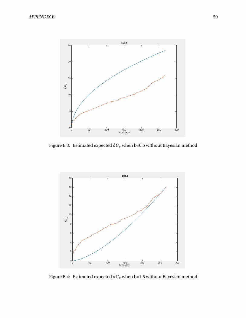
APPENDIX B. 59
Figure B.3: Estimated expected δCv when b=0.5 without Bayesian method
Figure B.4: Estimated expected δCv when b=1.5 without Bayesian method

APPENDIX B. 60
Figure B.5: Estimated expected δCv when b=2 without Bayesian method
Figure B.6: The plot of the choke B erosion indicator
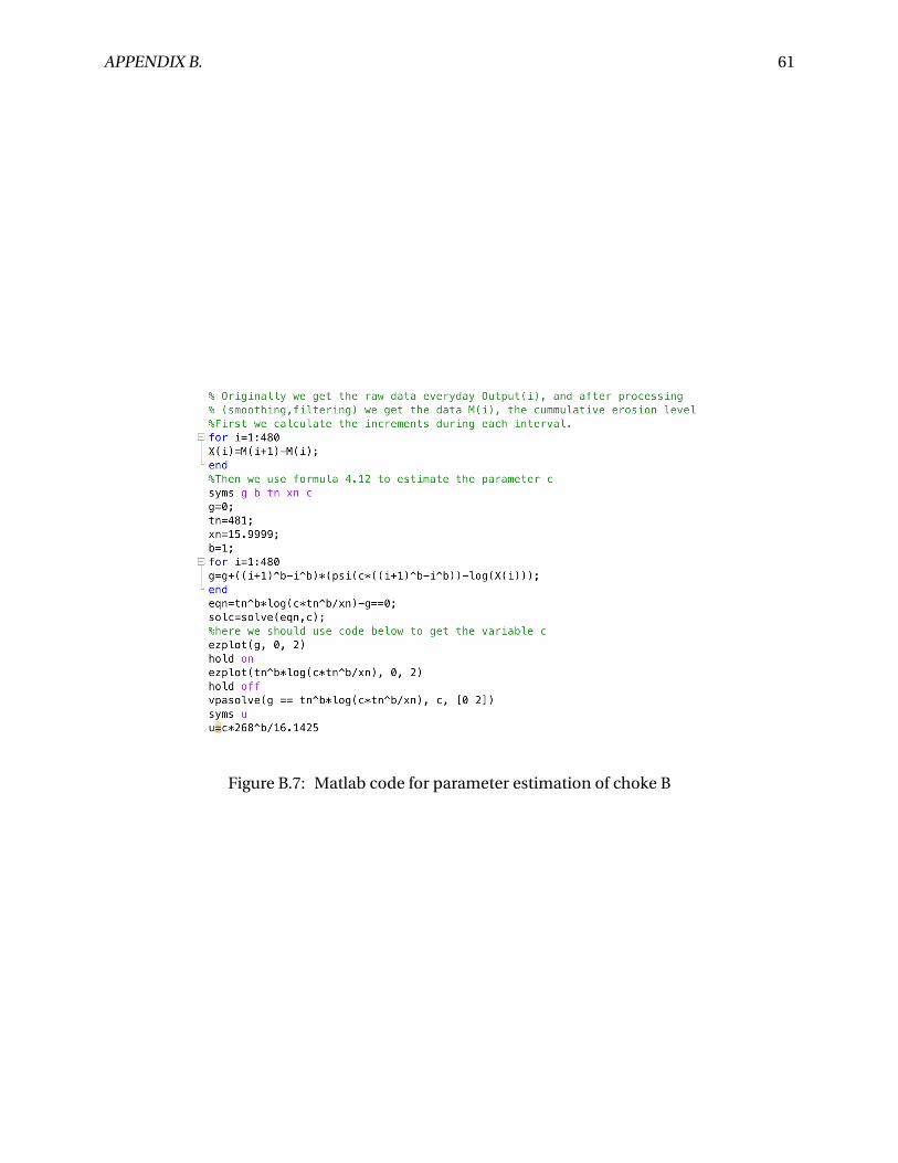
APPENDIX B. 61
Figure B.7: Matlab code for parameter estimation of choke B
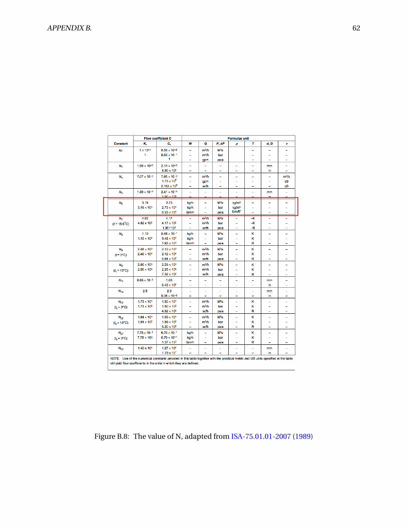
APPENDIX B. 62
Figure B.8: The value of N, adapted from ISA-75.01.01-2007 (1989)

Bibliography
A.Poongodai and S.Bhuvaneswari (2013). Ai technique in diagnostics and prognostics. Interna-
tional Journal of Computer Applications.
Austerlitz, H. (2002). Data Acquisition Techniques Using PCs. Academic Press.
Bazovsky, I. (1961). Reliability theory and practice. Prentice Hall, Englewood Cliffs, N.J.
Boden, M. (2001). A guide to recurrent neural networks and backpropagation.
Bostwick, D. G. and Burke, H. B. (2001). Prediction of individual patient outcome in cancer.
Cancer, 91.
Butler, S. . (2012). Prognostic Algorithms for Condition Monitoring and Remaining Useful Life
Estimation. PhD thesis, National University of Ireland Maynooth.
Byington, C. and Roemer, M. (2002). Prognostic enhancements to diagnostic systems for im-
proved condition-based maintenance [military aircraft]. In Aerospace Conference Proceedings,
2002. IEEE.
Cameron (2009). Subsea chokes-setting the industry standard, decade after decade. Technical
report, Cameron.
Carl S. Byington, P.E. Matthew Watson Byington, C. S., Watson, M., Edwards, D., and Stoelting,
P. (2004). A model-based approach to prognostics and health management for flight control
actuators. In Aerospace Conference, 2004. Proceedings. 2004 IEEE.
DWS team, D. T. G. Deflation warning system.
63

BIBLIOGRAPHY 64
E. Lunde, K. H. and Spjøtvold, J. (2010). Multi-disciplinary, multi-user process monitoring:
Cross-discipline development and cross-company collaboration. In SPE Intelligent Energy
Conference and Exhibition held in Utrecht, The Netherlands, 23–25 March 2010. SPE.
EMERSON (2010). Valve sizing calculations. Technical report, EMERSON.
Gallagher, N. B., Wise, B. M., Butler, S. W., White, D. D., Jr., and Barna, G. G. (1997). Development
and benchmarking of multivariate statistical process control tools for a semiconductor etch
process: Improving robustness through model updating.
Gebraeel, N., Lawley, M., Liu, R., and Parmeshwaran, V. (2004). Residual life predictions from
vibration-based degradation signals: a neural network approach. Industrial Electronics, IEEE
Transactions on, 51(3):694–700.
George Vachtsevanos, Frank L. Lewis, M. R. (2006). Intelligent Fault Diagnosis and Prognosis for
Engineering Systems. Wiley.
Heng, A., Zhang, S., Tan, A. C., and Mathew, J. (2009). Rotating machinery prognostics: State of
the art, challenges and opportunities. Mechanical Systems and Signal Processing, 23(3):724 –
739.
Hess, A., Calvello, G., Frith, P., and Engel (2006). Challenges, issues, and lessons learned chasing
the “big p”: real predictive prognostics part 2. Aerospace Conference, 2006 IEEE.
ISA-75.01.01-2007 (1989). Flow equations for sizing control valves,. In Standards and Recom-
mended Practices for Instrumentation and Control, volume 2.
ISO (2012). Iso 13372:2012 condition monitoring and diagnostics of machines – vocabulary.
J. Durbin., J. K. (2012). Time Series Analysis by State Space Methods. Oxford Statistical Science.
Jardine, A., Banjevic, D., Wiseman, M., Buck, S., and Joseph, T. (2001). Optimizing a mine haul
truck wheel motors’ condition monitoring program use of proportional hazards modeling.
Journal of Quality in Maintenance Engineering, 7(4):286–302.
Jardine, A. K. (1973). Maintenance, Replacement, and Reliabilitt. Wiley.
BIBLIOGRAPHY 65
Jardine, A. K., Lin, D., and Banjevic, D. (2006). A review on machinery diagnostics and prognos-
tics implementing condition-based maintenance. Mechanical Systems and Signal Processing,
20(7):1483 – 1510.
J.M. van Noortwijk, M. P. (2004). A stochastic deterioration process for time-dependent reliabil-
ity analysis. Reliability and optimization of structural systems, pages 259–265.
Kalgren, P., Byington, C., and Roemer, M. (2006). Defining phm, a lexical evolution of mainte-
nance and logistics. IEEE.
Kumar, D. and Westberg, U. (1996). Proportional hazards modeling of time-dependent covari-
ates using linear regression: a case study [mine power cable reliability]. Reliability, IEEE
Transactions on, 45(3).
Lawless, J. and Crowder, M. (2004). Covariates and random effects in a gamma process model
with application to degradation and failure. Lifetime Data Analysis, 10(3).
Lee, J., Wu, F., Zhao, W., Ghaffari, M., Liao, L., and Siegel, D. (2014). Prognostics and health
management design for rotary machinery systems—reviews, methodology and applications.
Mechanical Systems and Signal Processing, 42(1–2):314 – 334.
Li, C., Tao, L., and Yongsheng, B. (2007). Condition residual life evaluation by support vector
machine. Electronic Measurement and Instruments, 2007. ICEMI ’07. 8th International Con-
ference on.
Li, Y. and Nilkitsaranont, P. (2009). Gas turbine performance prognostic for condition-based
maintenance. Applied Energy, 86(10):2152 – 2161.
Nikolay V. Kirianaki, Sergey Y. Yurish, N. O. S. (2002). Data Acquisition and Signal Processing for
Smart Sensors. Wiley.
Pandey, M., Yuan, X., and Van Noortwijk, J. (2005). Gamma process model for reliability analysis
and replacement of aging structural components. Proceedings ICOSSAR, Rome, Italy, page
311.
BIBLIOGRAPHY 66
Peri, S. and Rogers, B. M. (2007). Computational fluid dynamics (cfd) erosion study for chokes.
In International Petroleum Technology Conference. International Petroleum Technology Con-
ference.
Qin, S. J. (2009). Data-driven fault detection and diagnosis for complex industrial processes.
Fault Detection, Supervision and Safety of Technical Processes.
Rausand, M. and Høyland, A. (2004). System Reliability Theory: Models, Statistical Methods, and
Applications. Wiley, Hoboken, NJ, 2nd edition.
Sæther, J. H. (2010). Choke condition and performance monitoring. Master’s thesis, Norwegian
University of Science and Technology.
Schwabacher, M. and Goebel, K. (2007). A survey of artificial intelligence for prognostics.
Thong, R. S. K. L. Y. L. (2000). Opening the neural network black box: an algorithm for extracting
rules from function approximating artificial neural networks. Proceedings of international
conference on Information systems, pages 176–186.
Vachtsevanos, G. and Wang, P. (2001). Fault prognosis using dynamic wavelet neural networks.
IEEE Systems Readiness Technology Conference, pages 857–870.
van Noortwijk, J. (2009). A survey of the application of gamma processes in maintenance. Reli-
ability Engineering System Safety, 94(1):2 – 21. Maintenance Modeling and Application.
Venkatasubramanian, V., Rengaswamy, R., Kavuri, S. N., and Yin, K. (2003). A review of pro-
cess fault detection and diagnosis: Part iii: Process history based methods. Computers and
Chemical Engineering, 27(3):327 – 346.
Veritas, D. N. (2007). Det Norske Veritas Recommended Practice RP0501 Erosive Wear In Piping
Systems, Revision4.2-2007. Det Norske Veritas.
Widodo, A. and Yang, B.-S. (2007). Support vector machine in machine condition monitoring
and fault diagnosis. Mechanical Systems and Signal Processing, 21(6):2560 – 2574.

BIBLIOGRAPHY 67
Wu, S.-j., Gebraeel, N., Lawley, M. A., and Yih, Y. (2007a). A neural network integrated decision
support system for condition-based optimal predictive maintenance policy. Systems, Man
and Cybernetics, Part A: Systems and Humans,, 37(2).
Wu, W., Hu, J., and Zhang, J. (2007b). Prognostics of machine health condition using an im-
proved arima-based prediction method. In Industrial Electronics and Applications, 2007.
ICIEA 2007. 2nd IEEE.

Curriculum Vitae
Name: Jie Zhang
Gender: Male
Date of birth: 11. January 1989
Address: Herman Krags Vei 15, 23, Moholt–7050 Trondheim
Nationality: Chinese
Email (1): [email protected]
Email (2): [email protected]
Telephone: +47 94433057
Language Skills
English: professional working proficiency (IELTS: overall: 7.0)
Norwegian: level 2
Education
• 2013.08 - 2015.07 Norwegian University of Science and Technology
RAMS Engineering (Reliability, Availability, Maintainability and Safety) GPA: B
• 2008.09 - 2012.07 China University of Geosciences (Beijing)
Safety Engineering GPA: 3.4 / 4.0 (87/100)
68

BIBLIOGRAPHY 69
Computer Skills
• Visual Basic, C Language, Python
• Minitab, SMILE, CARA Fault Tree, RCM++
• AutoCAD, PyroSim, Eclipse (basic), PLC (basic)
Experience
• 2015.01-2015.06 Norwegian University of Science and Technology
Title: Student Assistant (RAMS Engineering and Management Course)
• 2013.01-2015.06 Tsinghua Urban Planning and Design Institute
Title: Fire protection design engineer
-Proficiency in using PyroSim (Fluid Dynamics Simulation) Software
-Analysed the fire development, smoke and heat transmission
-Technically support for developing fire protection strategy
-Involved in projects Kunming Historical Block Fire Safety Risks Analysis, and Fire Preven-
tion and Control Planning of Gu Lei Port Economic Development Zone
Hobbies and Other Activities
• 2015.02 - 2015.02 Volunteer of introducing Chinese Culture in Trondheim
• 2014.10 - 2014.10 Your Extreme 2014 held by Kongsberg
• 2014.08 - 2014.08 Volunteer of Coralua Trondheim International Choir Festival
• 2009.05 - 2014.10 Volunteer of Chinese 60th anniversary celebration parade phalanx
• 2008.09 - 2010.07 President of Class 024081
-Organised more than 25 collective activities, including two New Year Galas.
-Held about 30 class meetings, including safety education, award selection work, learning

BIBLIOGRAPHY 70
experience sharing conferences.
- Be awarded Top 10 Class of our University (10/240) Good Style of Class (20/240)
• 2008.09 - 2009.07 Member of University Modern Drama Troupe
• 2008.09 - 2009.07 Member of Table Tennis Team and Badminton Team
Hobbies: Badminton, Basketball, Hiking, Swimming, Skiing, Table tennis, Photography