i © Copyright 2021 Xiaotian Li

i

© Copyright 2021

Xiaotian Li

ii

Agent-Based Parallelization of a Multi-Dimensional Semantic Database Model

Xiaotian Li

A whitepaper

submitted in partial fulfillment of the

requirements for the degree of

Master of Science in Computer Science & Software Engineering

University of Washington

May 2021

Project Committee:

Munehiro Fukuda, Ph.D., Committee Chair

Min Chen, Ph.D., Committee Member

Bill Erdly, Ph.D., Committee Member

iii

University of Washington

Abstract

Agent-Based Parallelization of a Multi-Dimensional Semantic Database Model

Xiaotian Li

Chair of the Supervisory Committee: Dr. Munehiro Fukuda

Computing and Software Systems

In conventional database systems, people consistently ignore the semantic meaning in autonomous

databases. It is not easy to extract significant information based on different querying contexts

from a database system. Mathematical Model of Meaning (MMM) is a meta database system that

extracts features from the database and explains the database by those features. It provides users

with the capabilities to extract significant information under different semantic spaces. The

semantic space is created dynamically with user-defined impression words to compute semantic

equivalence and similarity between data items. MMM computes semantic correlations between

the key data item and other data items to achieve dynamic data querying.

Multi-Agent Spatial Simulation library (MASS) is a parallel programming library that utilizes an

agent-based model (ABM) to parallelize extensive data analysis. This project presents parallel

iv

solutions to improve the performance of MMM using MASS. Multiple agent-based parallel

solutions were implemented to improve the efficiency of MMM. Compared to the sequential

MMM program, the parallel solution using MASS achieved 23 times speedup over the sequential

program on matrix multiplication. MASS also reduced the processing time of distance sorting of

multidimensional vectors by 23.70%. Additionally, this work also conducted benchmark analysis

and programmability analysis between MASS and MPI Java to indicate the advantages of agent-

based behavior.

v

v

TABLE OF CONTENTS

List of Figures ............................................................................................................................... vii

List of Tables ............................................................................................................................... viii

Chapter 1. Introduction ................................................................................................................... 9

1.1 Motivation ....................................................................................................................... 9

1.2 Project Goals and Achievements .................................................................................. 10

1.3 Structure of White Paper ............................................................................................... 12

Chapter 2. Background ................................................................................................................. 12

2.1 Mathematical Model of Meaning .................................................................................. 12

2.1.1 Correlation Matrix Calculation ................................................................................. 13

2.1.2 User-Defined Subspace Extraction with Eigen Decomposition ............................... 14

2.1.3 Sorting the Data Items by Calculating Euclidean Distance ...................................... 16

2.2 MASS ............................................................................................................................ 16

2.2.1 Place .......................................................................................................................... 17

2.2.2 Agent ......................................................................................................................... 18

Chapter 3. Related Works ............................................................................................................. 19

3.1 Parallel Database ........................................................................................................... 19

3.2 Semantic Database ........................................................................................................ 20

3.3 Summary ....................................................................................................................... 21

Chapter 4. Parallelization .............................................................................................................. 22

vi

vi

4.1 Sequential Results of MMM ......................................................................................... 22

4.2 Step I: Matrix Multiplication ........................................................................................ 23

4.2.1 Cannon's Algorithm .................................................................................................. 23

4.2.2 Parallel I/O ................................................................................................................ 26

4.3 STEP II: Eigen Decomposition ..................................................................................... 28

4.3.1 Householder Transformation .................................................................................... 28

4.3.2 Parallelization of Eigen Decomposition ................................................................... 29

4.4 STEP III: Euclidean distance sort of multi-dimensional vectors .................................. 30

4.4.1 Parallelization Algorithm .......................................................................................... 30

4.4.2 File I/O with RandomAccessFile .............................................................................. 33

Chapter 5. Results ......................................................................................................................... 34

5.1 Execution Environment ................................................................................................ 34

5.2 Matrix Multiplication .................................................................................................... 34

5.2.1 Computation Results ................................................................................................. 34

5.2.2 MASS Programmability Analysis ............................................................................ 36

5.3 Multi-Dimensional Vector Distance Sorting ................................................................ 39

5.3.1 Computational Results .............................................................................................. 40

Chapter 6. Conclusion ................................................................................................................... 42

6.1 Achievement ................................................................................................................. 42

6.2 Future Work .................................................................................................................. 43

Bibliography ................................................................................................................................. 45

Appendix A ................................................................................................................................... 48

vii

vii

LIST OF FIGURES

Figure 2.1. Creation of Input Matrix ................................................................................. 14

Figure 2.2. Dynamic Semantic Spaces ............................................................................. 16

Figure 2.3. MASS Programming Model ........................................................................... 18

Figure 4.1. MASS Sequential Benchmarks ...................................................................... 23

Figure 4.2. Programming Model of Cannon's Algorithm [17] ......................................... 24

Figure 4.3. Sample Diagonal Matrix [21] ......................................................................... 29

Figure 4.4. Agent Propagation in Three-Dimensional Space. .......................................... 31

Figure 4.5. Agent Propagation in Multi-Dimensional Space. ........................................... 32

Figure 5.1. Matrix Multiplication Benchmarks ................................................................ 35

Figure 5.2. Deadlocks in MPI ........................................................................................... 39

Figure 5.3. Data Sorting with Memory Space .................................................................. 40

Figure 5.4. Data Sorting with Random Access File .......................................................... 41

viii

viii

LIST OF TABLES

Table 5.1. Execution Time with Different Data Size and Levels ..................................... 41

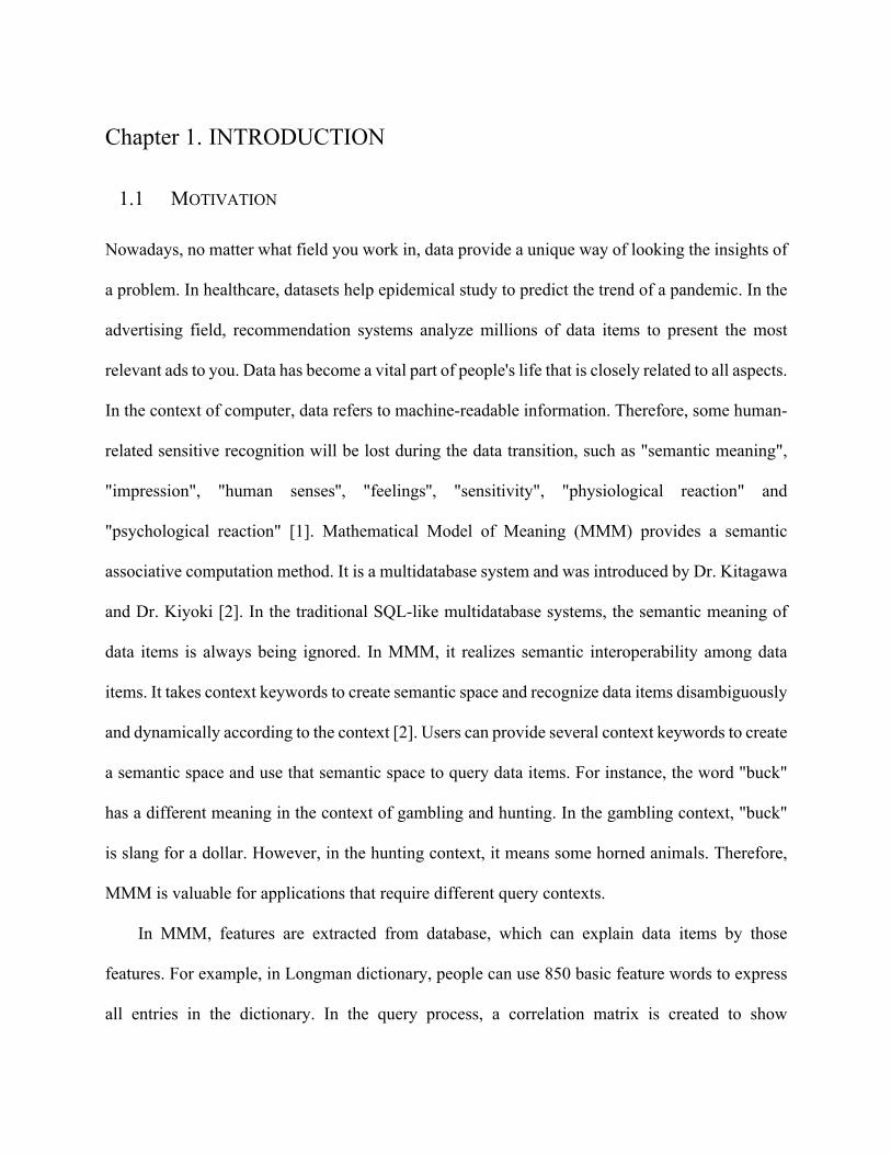
Chapter 1. INTRODUCTION

1.1 MOTIVATION

Nowadays, no matter what field you work in, data provide a unique way of looking the insights of

a problem. In healthcare, datasets help epidemical study to predict the trend of a pandemic. In the

advertising field, recommendation systems analyze millions of data items to present the most

relevant ads to you. Data has become a vital part of people's life that is closely related to all aspects.

In the context of computer, data refers to machine-readable information. Therefore, some human-

related sensitive recognition will be lost during the data transition, such as "semantic meaning",

"impression", "human senses'', "feelings'', "sensitivity", "physiological reaction" and

"psychological reaction" [1]. Mathematical Model of Meaning (MMM) provides a semantic

associative computation method. It is a multidatabase system and was introduced by Dr. Kitagawa

and Dr. Kiyoki [2]. In the traditional SQL-like multidatabase systems, the semantic meaning of

data items is always being ignored. In MMM, it realizes semantic interoperability among data

items. It takes context keywords to create semantic space and recognize data items disambiguously

and dynamically according to the context [2]. Users can provide several context keywords to create

a semantic space and use that semantic space to query data items. For instance, the word "buck"

has a different meaning in the context of gambling and hunting. In the gambling context, "buck"

is slang for a dollar. However, in the hunting context, it means some horned animals. Therefore,

MMM is valuable for applications that require different query contexts.

In MMM, features are extracted from database, which can explain data items by those

features. For example, in Longman dictionary, people can use 850 basic feature words to express

all entries in the dictionary. In the query process, a correlation matrix is created to show

10

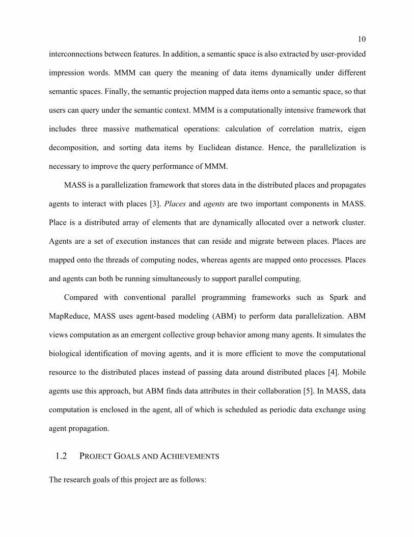
interconnections between features. In addition, a semantic space is also extracted by user-provided

impression words. MMM can query the meaning of data items dynamically under different

semantic spaces. Finally, the semantic projection mapped data items onto a semantic space, so that

users can query under the semantic context. MMM is a computationally intensive framework that

includes three massive mathematical operations: calculation of correlation matrix, eigen

decomposition, and sorting data items by Euclidean distance. Hence, the parallelization is

necessary to improve the query performance of MMM.

MASS is a parallelization framework that stores data in the distributed places and propagates

agents to interact with places [3]. Places and agents are two important components in MASS.

Place is a distributed array of elements that are dynamically allocated over a network cluster.

Agents are a set of execution instances that can reside and migrate between places. Places are

mapped onto the threads of computing nodes, whereas agents are mapped onto processes. Places

and agents can both be running simultaneously to support parallel computing.

Compared with conventional parallel programming frameworks such as Spark and

MapReduce, MASS uses agent-based modeling (ABM) to perform data parallelization. ABM

views computation as an emergent collective group behavior among many agents. It simulates the

biological identification of moving agents, and it is more efficient to move the computational

resource to the distributed places instead of passing data around distributed places [4]. Mobile

agents use this approach, but ABM finds data attributes in their collaboration [5]. In MASS, data

computation is enclosed in the agent, all of which is scheduled as periodic data exchange using

agent propagation.

1.2 PROJECT GOALS AND ACHIEVEMENTS

The research goals of this project are as follows:

11

1) Reimplement MMM using Java and collect sequential performance benchmarks.

MMM was first introduced in 1993, the software and hardware performance have been

improved a lot since then. We want to evaluate the performance of MMM to see which part

takes the most time of the application so that we will get a better idea of the parallelization

strategy.

2) Enhance the overall performance of MMM by applying MASS. We implemented four

algorithms to parallelize MMM using agent-based approaches. We also conduct five

benchmark analyses to evaluate performance improvement compared with the sequential

program. In addition, we also compared MASS with MPI Java for some parts of the

parallelization, which reveals MASS's strengths to some data streaming problems.

3) Prove applicability of MASS in a real-world problem. Before we started this project,

MASS was used for analyzing large datasets and paralleling data-science applications.

MASS shows excellent performance when compared with other frameworks such as MPI,

MapReduce, and Spark [5]. However, MASS hasn't approved much on real-world

problems. This project gives us an opportunity to explore how MASS will perform when

solving those problems.

In our work, we split MMM into three different steps and implemented the MMM using Java.

By analyzing the execution performance of MMM, we identified the performance bottleneck

within it. Therefore, agent-based parallelization approaches with MASS were applied to MMM,

which gave us a satisfactory result compared with sequential performance. The execution time of

matrix multiplication using MASS improved by 95% in comparison with the sequential program

and the distance sort of multidimensional vectors also improved by 24%. The details of our

achievements can be viewed in Chapter 5.

12

1.3 STRUCTURE OF WHITE PAPER

The rest of this white paper is organized as follows: Chapter 2 introduces the background of MMM

and MASS. Chapter 3 reviews related works of semantic database and parallel database. Chapter

4 discusses the related parallelization strategy of different steps in MMM. Chapter 5 presents the

benchmarks analysis as well as the programmability analysis of MASS's implementations. At last,

Chapter 6 concludes the project with future enhancements and limitations.

Chapter 2. BACKGROUND

2.1 MATHEMATICAL MODEL OF MEANING

The relational database is unarguably the most popular database model today. It has been widely

used in almost every field that needs to save structural data. As in relational databases such as

SQL, database model designers have to convert data interconnections to computer language, which

requires an additional direction. In addition, relational database also shows weakness in capturing

the semantic meaning of data items. During a data querying process, the results from relational

database are usually abstracted and returned to unnatural structural relationships. These

relationships are always defined by the pre-defined foreign key declarations [6]. It always captures

the logical relationship but ignores the natural semantic structures.

In a database, the semantics usually refer to three major categories: formal semantics, lexical

semantics, and conceptual semantics [6]. The formal semantics means the feeling and sense of

people. The lexical semantics represents the underlying meaning of a word and data item, and the

conceptual semantics usually indicates the cognitive structure of data items. In order to realize the

semantic meaning in the database, it not only focuses on the underlying meaning of data items but

also the relationship of what they stand for. Data items always cannot be identified independently.

13

MMM is a semantic database model that helps users to discover data items with equivalent or

similar meanings. In the normal SQL-like database, a data item is queried by pattern matching.

The SELECT and WHERE clauses are used to filter data items through user-provided conditions.

Comparing with a SQL-like database, the data item is queried by semantic associative search

where data items are projected onto semantic spaces. MMM calculates the Euclidean distance

between data items to find out the most relevant data items based on user-selected semantic spaces.

The following sections present the technical details of three steps in MMM and discuss how does

semantic associative work in MMM.

2.1.1 Correlation Matrix Calculation

Overall, MMM can be separated into three different steps. The first step is to formalize the initial

input data into matrix A, which is an m rows by n columns matrix. In this matrix, each feature is

translated into a column, and each data item is represented as a row in a matrix. To create the initial

input matrix, we refer to the basic words that explain all the dictionary's vocabulary entries as

features. For example, the word "nice" can be expressed by features "kind", "nice" and "friend"

and the word "small" can be expressed by features "amount", "average", "importance", "-large",

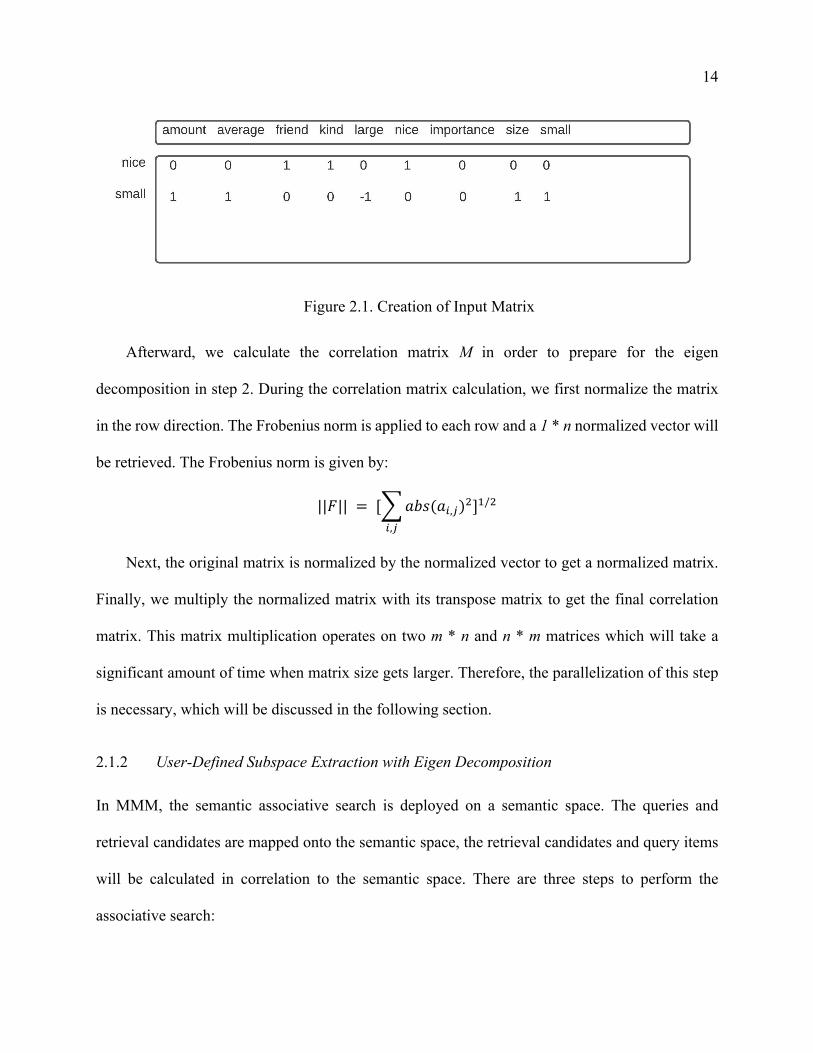
"size" and "small" itself. Figure 2.1 shows a matrix to use n features to explain all m words. For

example, in the word "nice", each feature word is set to 1 to illustrate the positive relationship

between feature word and data word. In the case of "small", the negative value "-1" is set on the

column of "large" to explain the negative value of this column. If features are not used to explain

vocabulary terms, the columns corresponding to those features are set to "0" [1].

14

Figure 2.1. Creation of Input Matrix

Afterward, we calculate the correlation matrix M in order to prepare for the eigen

decomposition in step 2. During the correlation matrix calculation, we first normalize the matrix

in the row direction. The Frobenius norm is applied to each row and a 1 * n normalized vector will

be retrieved. The Frobenius norm is given by:

||𝐹|| = [&𝑎𝑏𝑠(𝑎!,#)$!,#

]%/$

Next, the original matrix is normalized by the normalized vector to get a normalized matrix.

Finally, we multiply the normalized matrix with its transpose matrix to get the final correlation

matrix. This matrix multiplication operates on two m * n and n * m matrices which will take a

significant amount of time when matrix size gets larger. Therefore, the parallelization of this step

is necessary, which will be discussed in the following section.

2.1.2 User-Defined Subspace Extraction with Eigen Decomposition

In MMM, the semantic associative search is deployed on a semantic space. The queries and

retrieval candidates are mapped onto the semantic space, the retrieval candidates and query items

will be calculated in correlation to the semantic space. There are three steps to perform the

associative search:

15

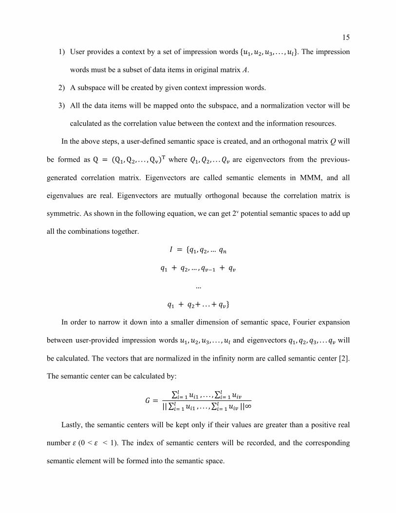
1) User provides a context by a set of impression words {𝑢%, 𝑢$, 𝑢', . . . , 𝑢(}. The impression

words must be a subset of data items in original matrix A.

2) A subspace will be created by given context impression words.

3) All the data items will be mapped onto the subspace, and a normalization vector will be

calculated as the correlation value between the context and the information resources.

In the above steps, a user-defined semantic space is created, and an orthogonal matrix Q will

be formed as Q = (Q%, Q$, . . . , Q))* where 𝑄%, 𝑄$, . . . 𝑄+are eigenvectors from the previous-

generated correlation matrix. Eigenvectors are called semantic elements in MMM, and all

eigenvalues are real. Eigenvectors are mutually orthogonal because the correlation matrix is

symmetric. As shown in the following equation, we can get 2v potential semantic spaces to add up

all the combinations together.

𝐼 = {𝑞%, 𝑞$, …𝑞,

𝑞% + 𝑞$, … , 𝑞+-% + 𝑞+

…

𝑞% + 𝑞$+. . . +𝑞+}

In order to narrow it down into a smaller dimension of semantic space, Fourier expansion

between user-provided impression words 𝑢%, 𝑢$, 𝑢', . . . , 𝑢( and eigenvectors 𝑞%, 𝑞$, 𝑞', . . . 𝑞+will

be calculated. The vectors that are normalized in the infinity norm are called semantic center [2].

The semantic center can be calculated by:

𝐺 = ∑ 𝑢!%(!.% , . . . , ∑ 𝑢!+(

!.%

|| ∑ 𝑢!%(!.% , . . . , ∑ 𝑢!+(

!.% ||∞

Lastly, the semantic centers will be kept only if their values are greater than a positive real

number 𝜀 (0 < 𝜀 < 1). The index of semantic centers will be recorded, and the corresponding

semantic element will be formed into the semantic space.

16

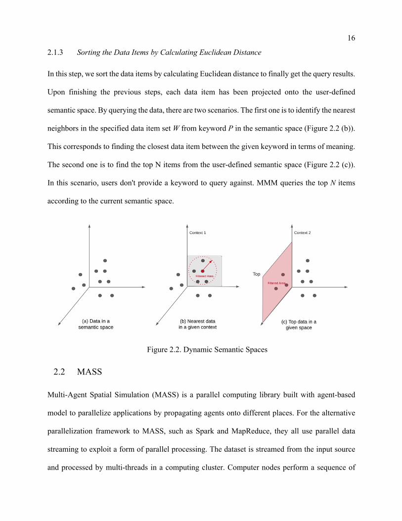
2.1.3 Sorting the Data Items by Calculating Euclidean Distance

In this step, we sort the data items by calculating Euclidean distance to finally get the query results.

Upon finishing the previous steps, each data item has been projected onto the user-defined

semantic space. By querying the data, there are two scenarios. The first one is to identify the nearest

neighbors in the specified data item set W from keyword P in the semantic space (Figure 2.2 (b)).

This corresponds to finding the closest data item between the given keyword in terms of meaning.

The second one is to find the top N items from the user-defined semantic space (Figure 2.2 (c)).

In this scenario, users don't provide a keyword to query against. MMM queries the top N items

according to the current semantic space.

Figure 2.2. Dynamic Semantic Spaces

2.2 MASS

Multi-Agent Spatial Simulation (MASS) is a parallel computing library built with agent-based

model to parallelize applications by propagating agents onto different places. For the alternative

parallelization framework to MASS, such as Spark and MapReduce, they all use parallel data

streaming to exploit a form of parallel processing. The dataset is streamed from the input source

and processed by multi-threads in a computing cluster. Computer nodes perform a sequence of

17

operations on the data stream in parallel and return the results to the downstream. In this way, each

individual request has to go through the whole process of data streaming.

On the other hand, with agent-based approach, MASS is able to save the data into a dedicated

area so that further agents can retrieve data on demand. In addition, the database system requires

the parallelization framework should be able to analyze data on the fly. Once the system receives

a query request, the parallelization framework should minimize the data-reading process. MASS

can also satisfy this requirement by spawning new agents to take charge of new requests. In MASS,

there are two major components, Places and Agents. In the following sections, we will discuss the

programming model of MASS as well as the main functionalities of places and agents.

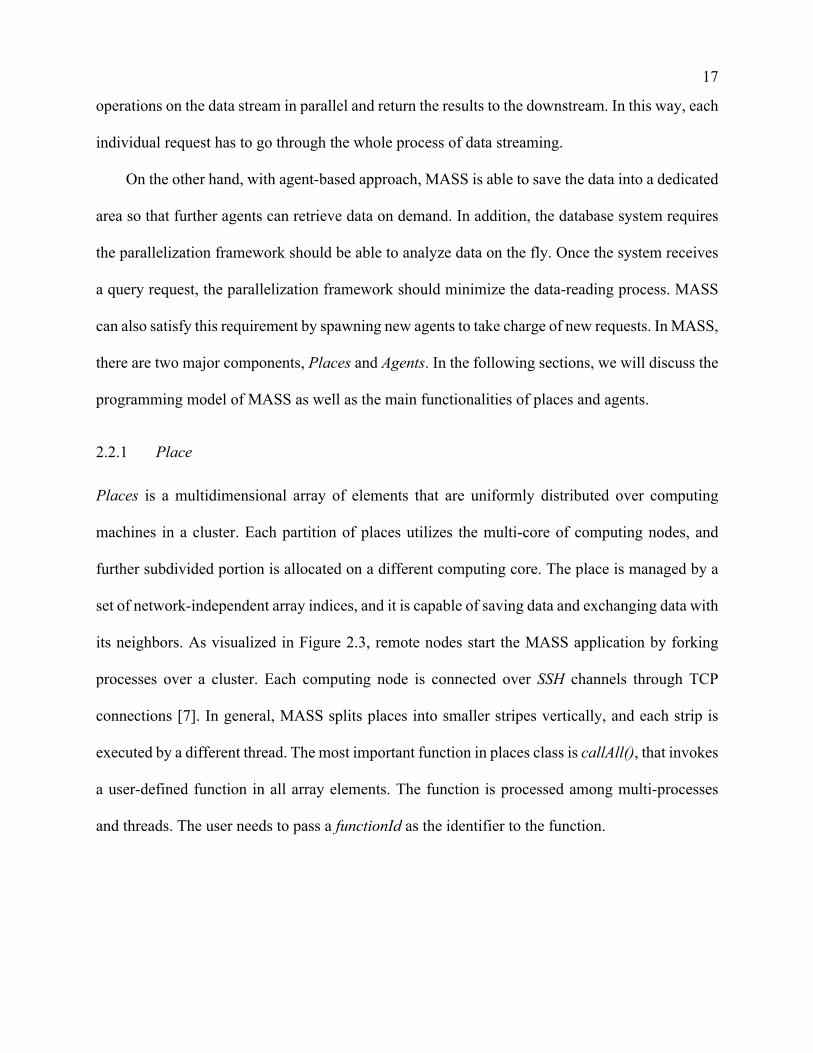
2.2.1 Place

Places is a multidimensional array of elements that are uniformly distributed over computing

machines in a cluster. Each partition of places utilizes the multi-core of computing nodes, and

further subdivided portion is allocated on a different computing core. The place is managed by a

set of network-independent array indices, and it is capable of saving data and exchanging data with

its neighbors. As visualized in Figure 2.3, remote nodes start the MASS application by forking

processes over a cluster. Each computing node is connected over SSH channels through TCP

connections [7]. In general, MASS splits places into smaller stripes vertically, and each strip is

executed by a different thread. The most important function in places class is callAll(), that invokes

a user-defined function in all array elements. The function is processed among multi-processes

and threads. The user needs to pass a functionId as the identifier to the function.

18

Figure 2.3. MASS Programming Model

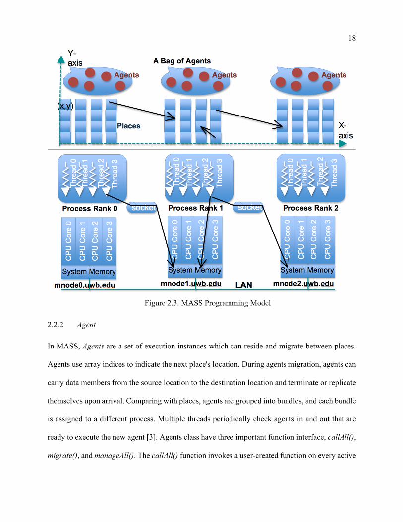
2.2.2 Agent

In MASS, Agents are a set of execution instances which can reside and migrate between places.

Agents use array indices to indicate the next place's location. During agents migration, agents can

carry data members from the source location to the destination location and terminate or replicate

themselves upon arrival. Comparing with places, agents are grouped into bundles, and each bundle

is assigned to a different process. Multiple threads periodically check agents in and out that are

ready to execute the new agent [3]. Agents class have three important function interface, callAll(),

migrate(), and manageAll(). The callAll() function invokes a user-created function on every active

19

agent, and the user-created function is pointed by functionId. migrate() function initiates an agent

migration to a new place by calling places index. manageAll() function updates the status of an

agent. Under the hood of manageAll() function, it checks the size of each agent bag and

synchronizes all threads together. The most recent version of MASS also supports event-driven

agent behaviors to allow users to associate functions upon agents' departure, arrival, and creation.

Each of them is annotated as @OnDeparture, @OnArrival, and @OnCreation [8].

Chapter 3. RELATED WORKS

This chapter describes the existing semantic database and parallelized database. It discusses the

advantage of our approach and the limitations of past research.

3.1 PARALLEL DATABASE

Parallel database has been widely adopted by data-intensive applications. It provides optimized

performance and high scalability compared with traditional database. In the traditional database,

the size of disk space and memory space always limits the number of data items that can be fit in

a database. As data size grows bigger, parallel database can store the data item in a distributed

fashion and improve its processing speed with multiple computing nodes and CPUs. In the parallel

database system, where operations are performed simultaneously, a single task can be distributed

onto multiple nodes and combine results by finishing the task.

There are three types of architecture for parallel machines. They are shared-disk, shared-

memory, and shared-nothing architectures [9]. Shared-memory architecture typically means that

all computer nodes share a global memory space. In [10], authors proposed multiple algorithms

that use remote direct memory (RDMA) in parallel database system. The work dynamically

manages RMDA-registered memory to improve the database performance. A shared-disk parallel

20

database system was proposed in [11]. The shared-disk system has a low communication overhead

compared to other architectures. Especially for the reading actions, the operations can spread over

multiple nodes to shorten the response time. It provides flexibility for the reading operations.

Our proposed MMM and MASS integrated solution is a shared-nothing architecture. The

advantage of shared-nothing architecture is high extensibility and high availability. Compare with

other shared-nothing architecture, such as MySQL Cluster, MASS is easier to scale up the system

without considering data partitioning. The data can be fed into places of new machines instead of

syncing up with previously existing nodes. In addition, our solution also eliminates single points

of failure. With agent-based approach, a single failure will only cause some agents to be terminated

but other agents can continue work on their tasks. Moreover, MASS is capable to operate multiple

concurrent requests and analyze data on the fly. Once places are initialized, agents can make use

of the initialized data to do operations and analysis and concurrent requests can be handled by new

spawned agents. Our solution is more flexible and reliable compared to other discussed work.

3.2 SEMANTIC DATABASE

In 1978, Semantic Data Model (SDM) was firstly introduced by Michael Hammer, which provides

a high-level semantic-based modeling mechanism to capture and express the structural formalism

for databases [12]. SDM facilitates data querying from different perspectives, where users can

query data by declaring their views of a large database. Although SDM leads to some redundancy

of data storage by providing multiple perspectives of a database, users can still benefit from its

enriched relationship schema to better understand the data in a natural way. In World Wide Web,

W3C introduced the standard of Web Ontology Language (OWL) and the Resource Description

Format (RDF) to realize a semantic web. The purpose of introducing a semantic web is to make

machines can understand and interpret complex human requests based on their meaning [13]. The

21

focus of OWL and RDF is known as triples, which is the form of subject-predicate-object. The

subject and object denote the resources, and the predicate tells the relationship between subject

and resources, as well as describes the traits or aspects of the resources. OWL and RDF utilize a

metadata model to express semantic meaning in web resources and various syntax notations to

make the semantic meaning understandable by machines. With the growing amount of web

information being processed and extracted, the most valuable and related information can be

filtered by domains. Also, the web crawler can be beneficial from the semantic web information.

In [14], a semantic-based model to represent big multimedia data is proposed. The work describes

a property-based graph that allows users to express the concept and relationship between

multimedia data items. A graph database is utilized to save key-value pairs of data items and

traverse their connections. Their work presents a machine-understandable representation that

organizes the semantic associations between multimedia data items.

Most semantic database models highly rely on either modeling information in a relational

database or modeling the resources and their relationship of data items [6][14]. In addition, some

semantic databases are limited to specific domains, and they usually don't provide a general

semantic database solution. In the vision of MMM, it doesn't rely on any relational database. A

group of features represents the value of data items. In addition, MMM can realize the dynamic

recognition of the context by a semantic projection that cannot be achieved by other discussed

literature.

3.3 SUMMARY

To summarize, our integrated system with MMM and MASS has the following advantages.

1) MMM, as a semantic database model, is a complete mathematical model. MMM doesn't

require assistance from any other relational database or graphs to save the semantic

22

structure. MMM can use semantic projection and semantic associative search to realize

data search by semantic meaning under a different context.

2) By using the agent-based model in our system, the system can achieve the best scalability

and availability. Since MASS is based on shared-nothing architecture, we can add more

computing resources on demand. Therefore, the architecture will not set any obstacles

when scaling up the system.

Chapter 4. PARALLELIZATION

This chapter, it presents multiple agent-based parallelization algorithms, each applied to a different

MMM step. Additionally, it also discusses the sequential results of MMM, which are programmed

in Java.

4.1 SEQUENTIAL RESULTS OF MMM

We first implemented MMM using Java to retrieve the sequential benchmarks. The sequential

benchmarks are organized in 3 steps, as we previously mentioned.

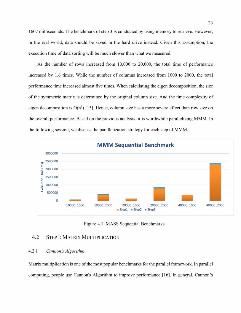
Figure 4.1 shows the execution time measured with System.currentTimeMillis() when

handling different sizes of datasets. The datasets are generated with random double values. Overall,

step 1 costs the most time in MMM. The matrix normalization and multiplication take over 90%

of the overall time. When the matrix size reaches 40000 rows and 2000 columns, it takes more

time than other datasets, which takes over 40 minutes to complete the calculation. As for step 2, it

accounts for 7% of the total time on average. It has the highest percentage of overall time when

the matrix size is at 10000 rows and 2000 columns, which is 17%. As of step 3, the performance

of sorting all data items is based on the distance between themselves and the key data item. The

benchmarks indicate step 3 has the smallest percentage of overall time, and the slowest one takes

23

1607 milliseconds. The benchmark of step 3 is conducted by using memory to retrieve. However,

in the real world, data should be saved in the hard drive instead. Given this assumption, the

execution time of data sorting will be much slower than what we measured.

As the number of rows increased from 10,000 to 20,000, the total time of performance

increased by 1.6 times. While the number of columns increased from 1000 to 2000, the total

performance time increased almost five times. When calculating the eigen decomposition, the size

of the symmetric matrix is determined by the original column size. And the time complexity of

eigen decomposition is O(n3) [15]. Hence, column size has a more severe effect than row size on

the overall performance. Based on the previous analysis, it is worthwhile parallelizing MMM. In

the following session, we discuss the parallelization strategy for each step of MMM.

Figure 4.1. MASS Sequential Benchmarks

4.2 STEP I: MATRIX MULTIPLICATION

4.2.1 Cannon's Algorithm

Matrix multiplication is one of the most popular benchmarks for the parallel framework. In parallel

computing, people use Cannon's Algorithm to improve performance [16]. In general, Cannon’s

0

500000

1000000

1500000

2000000

2500000

3000000

10000_1000 10000_2000 20000_1000 20000_2000 40000_1000 40000_2000

Exec

utio

n TI

me

(ms)

MMM Sequential Benchmark

Step1 Step2 Step3

24

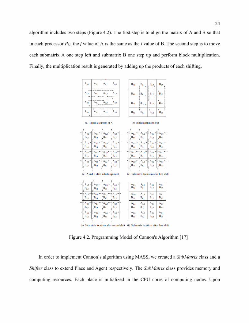
algorithm includes two steps (Figure 4.2). The first step is to align the matrix of A and B so that

in each processor Pi,j, the j value of A is the same as the i value of B. The second step is to move

each submatrix A one step left and submatrix B one step up and perform block multiplication.

Finally, the multiplication result is generated by adding up the products of each shifting.

Figure 4.2. Programming Model of Cannon's Algorithm [17]

In order to implement Cannon’s algorithm using MASS, we created a SubMatrix class and a

Shifter class to extend Place and Agent respectively. The SubMatrix class provides memory and

computing resources. Each place is initialized in the CPU cores of computing nodes. Upon

25

initialization, the place will read the data from the CSV file and save their corresponding portion

into the memory space.

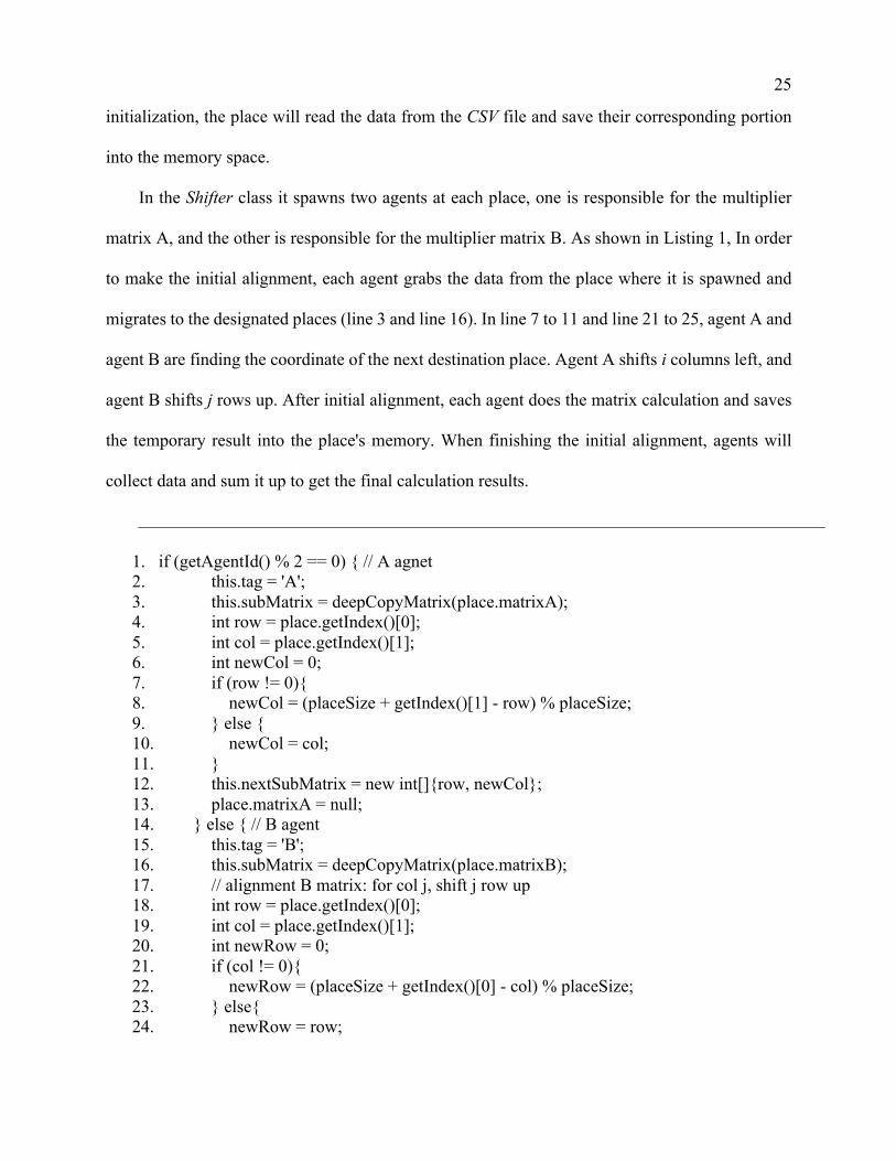
In the Shifter class it spawns two agents at each place, one is responsible for the multiplier

matrix A, and the other is responsible for the multiplier matrix B. As shown in Listing 1, In order

to make the initial alignment, each agent grabs the data from the place where it is spawned and

migrates to the designated places (line 3 and line 16). In line 7 to 11 and line 21 to 25, agent A and

agent B are finding the coordinate of the next destination place. Agent A shifts i columns left, and

agent B shifts j rows up. After initial alignment, each agent does the matrix calculation and saves

the temporary result into the place's memory. When finishing the initial alignment, agents will

collect data and sum it up to get the final calculation results.

1. if (getAgentId() % 2 == 0) { // A agnet 2. this.tag = 'A'; 3. this.subMatrix = deepCopyMatrix(place.matrixA); 4. int row = place.getIndex()[0]; 5. int col = place.getIndex()[1]; 6. int newCol = 0; 7. if (row != 0){ 8. newCol = (placeSize + getIndex()[1] - row) % placeSize; 9. } else { 10. newCol = col; 11. } 12. this.nextSubMatrix = new int[]{row, newCol}; 13. place.matrixA = null; 14. } else { // B agent 15. this.tag = 'B'; 16. this.subMatrix = deepCopyMatrix(place.matrixB); 17. // alignment B matrix: for col j, shift j row up 18. int row = place.getIndex()[0]; 19. int col = place.getIndex()[1]; 20. int newRow = 0; 21. if (col != 0){ 22. newRow = (placeSize + getIndex()[0] - col) % placeSize; 23. } else{ 24. newRow = row;

26

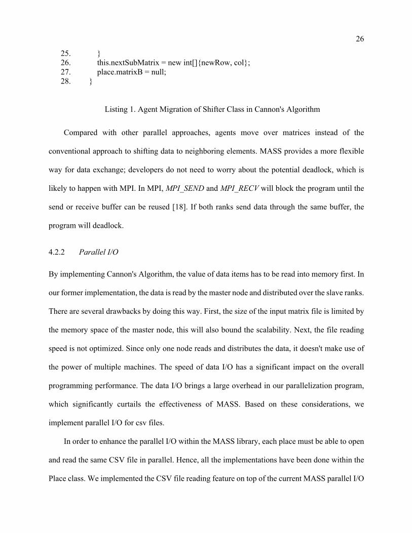
25. } 26. this.nextSubMatrix = new int[]{newRow, col}; 27. place.matrixB = null; 28. }

Listing 1. Agent Migration of Shifter Class in Cannon's Algorithm

Compared with other parallel approaches, agents move over matrices instead of the

conventional approach to shifting data to neighboring elements. MASS provides a more flexible

way for data exchange; developers do not need to worry about the potential deadlock, which is

likely to happen with MPI. In MPI, MPI_SEND and MPI_RECV will block the program until the

send or receive buffer can be reused [18]. If both ranks send data through the same buffer, the

program will deadlock.

4.2.2 Parallel I/O

By implementing Cannon's Algorithm, the value of data items has to be read into memory first. In

our former implementation, the data is read by the master node and distributed over the slave ranks.

There are several drawbacks by doing this way. First, the size of the input matrix file is limited by

the memory space of the master node, this will also bound the scalability. Next, the file reading

speed is not optimized. Since only one node reads and distributes the data, it doesn't make use of

the power of multiple machines. The speed of data I/O has a significant impact on the overall

programming performance. The data I/O brings a large overhead in our parallelization program,

which significantly curtails the effectiveness of MASS. Based on these considerations, we

implement parallel I/O for csv files.

In order to enhance the parallel I/O within the MASS library, each place must be able to open

and read the same CSV file in parallel. Hence, all the implementations have been done within the

Place class. We implemented the CSV file reading feature on top of the current MASS parallel I/O

27

implementations. In the new design of parallel I/O, it firstly opens the file by taking the given

filePath argument, which determines the file's name and whether the file's type is supported.

Currently, MASS parallel I/O supports NetCDF, TXT, and CSV files. If the given file type is not

supported, then -1 is returned. Otherwise, this file will be opened and saved into the fileTable. The

open method is a synchronized method so that only one place will perform the open task on

individual computing node. The file reading is implemented by splitting the file into an equal

number of bytes, and each computing node gets a corresponding portion. However, since each data

record's character length is different for the CSV file, directly splitting the file will make records

lose some digits. To solve this problem, we add paddings on each line to make sure they all have

the same length. In this case, when we split the file by an equal number of bytes, every computing

node gets the same number of rows. The following method is added in the CsvFile.java class,

which is used explicitly for handling CSV parallel I/O.

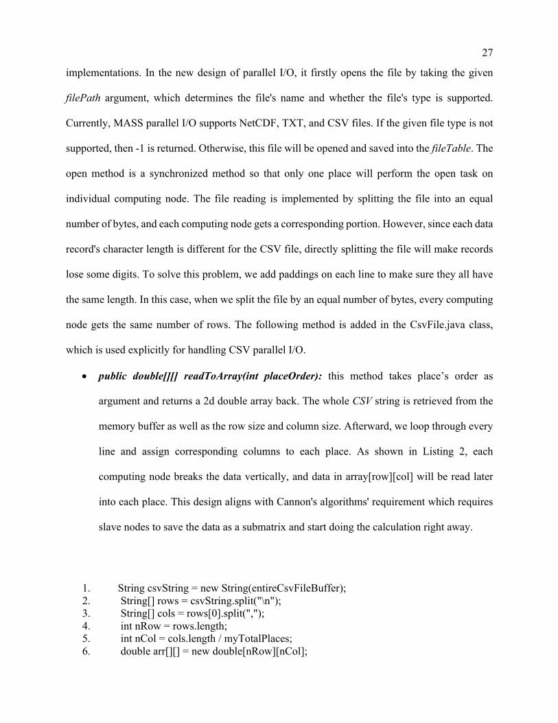
• public double[][] readToArray(int placeOrder): this method takes place’s order as

argument and returns a 2d double array back. The whole CSV string is retrieved from the

memory buffer as well as the row size and column size. Afterward, we loop through every

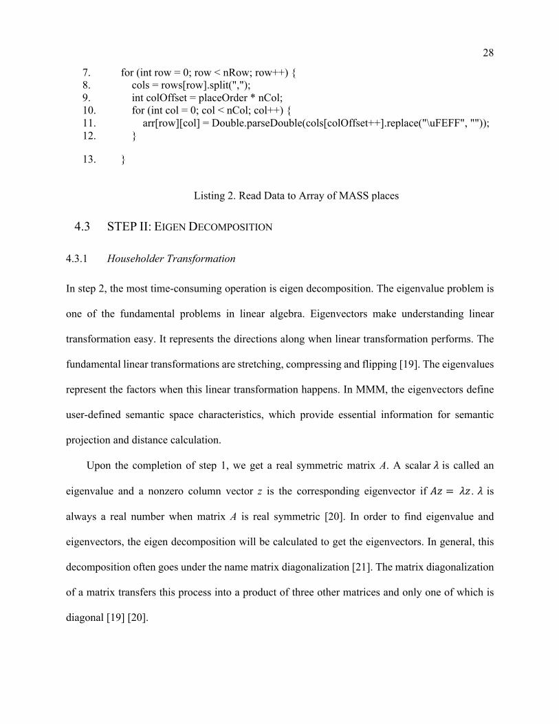
line and assign corresponding columns to each place. As shown in Listing 2, each

computing node breaks the data vertically, and data in array[row][col] will be read later

into each place. This design aligns with Cannon's algorithms' requirement which requires

slave nodes to save the data as a submatrix and start doing the calculation right away.

1. String csvString = new String(entireCsvFileBuffer); 2. String[] rows = csvString.split("\n"); 3. String[] cols = rows[0].split(","); 4. int nRow = rows.length; 5. int nCol = cols.length / myTotalPlaces; 6. double arr[][] = new double[nRow][nCol];

28

7. for (int row = 0; row < nRow; row++) { 8. cols = rows[row].split(","); 9. int colOffset = placeOrder * nCol; 10. for (int col = 0; col < nCol; col++) { 11. arr[row][col] = Double.parseDouble(cols[colOffset++].replace("\uFEFF", "")); 12. }

13. }

Listing 2. Read Data to Array of MASS places

4.3 STEP II: EIGEN DECOMPOSITION

4.3.1 Householder Transformation

In step 2, the most time-consuming operation is eigen decomposition. The eigenvalue problem is

one of the fundamental problems in linear algebra. Eigenvectors make understanding linear

transformation easy. It represents the directions along when linear transformation performs. The

fundamental linear transformations are stretching, compressing and flipping [19]. The eigenvalues

represent the factors when this linear transformation happens. In MMM, the eigenvectors define

user-defined semantic space characteristics, which provide essential information for semantic

projection and distance calculation.

Upon the completion of step 1, we get a real symmetric matrix A. A scalar 𝜆 is called an

eigenvalue and a nonzero column vector z is the corresponding eigenvector if 𝐴𝑧 = 𝜆𝑧 . 𝜆 is

always a real number when matrix A is real symmetric [20]. In order to find eigenvalue and

eigenvectors, the eigen decomposition will be calculated to get the eigenvectors. In general, this

decomposition often goes under the name matrix diagonalization [21]. The matrix diagonalization

of a matrix transfers this process into a product of three other matrices and only one of which is

diagonal [19] [20].

29

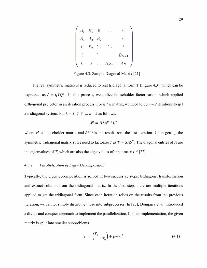
Figure 4.3. Sample Diagonal Matrix [21]

The real symmetric matrix A is reduced to real tridiagonal form T (Figure 4.3), which can be

expressed as 𝐴 = 𝑄𝑇𝑄0 . In this process, we utilize householder factorization, which applied

orthogonal projector in an iteration process. For n * n matrix, we need to do n – 2 iterations to get

a tridiagonal system. For k = 1, 2, 3, … n – 2 as follows:

𝐴1 = 𝐻1𝐴1-%𝐻1

where H is householder matrix and 𝐴1-% is the result from the last iteration. Upon getting the

symmetric tridiagonal matrix T, we need to factorize T as 𝑇 = 𝑆𝛬𝑆0. The diagonal entries of 𝛬 are

the eigenvalues of T, which are also the eigenvalues of input matrix A [22].

4.3.2 Parallelization of Eigen Decomposition

Typically, the eigen decomposition is solved in two successive steps: tridiagonal transformation

and extract solution from the tridiagonal matrix. In the first step, there are multiple iterations

applied to get the tridiagonal form. Since each iteration relies on the results from the previous

iteration, we cannot simply distribute those into subprocesses. In [23], Dongarra et al. introduced

a divide and conquer approach to implement the parallelization. In their implementation, the given

matrix is split into smaller subproblems.

𝑇 = C𝑇% 𝑇$D + 𝑝𝑤𝑤0 (4.1)

30

As shown in 4.1, the original input matrix is divided into two half-sized submatrices. For 1 ≤

𝑘 ≤ 𝑛, the 𝑇%and 𝑇$are the kth diagonal elements. When subproblems are small enough, the QR

refactor is called so that

𝑇% = 𝑄%Λ%𝑄%0 (4.2)

𝑇$ = 𝑄$Λ$𝑄$0 (4.3)

Finally, the backward computation will be called to form the tridiagonal matrix and compute

the eigenvectors of matrix T. Because of the time restriction of this project, we don't have chance

to implement this parallelization algorithm with MASS. We wish we can tackle this problem in

future.

4.4 STEP III: EUCLIDEAN DISTANCE SORT OF MULTI-DIMENSIONAL VECTORS

4.4.1 Parallelization Algorithm

In step 3 of MMM, it requires sorting data items by the distance from the key data item to others.

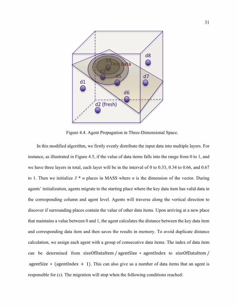
In our original proposal, we wanted to use agent propagation for the parallelization

implementation. An agent spawns at the location of a test data item. They will propagate to the

surrounding places until one agent collides with others. As shown in Figure 4.4, this approach

works well in one-dimension to three-dimensional spaces. However, it would be tough to find out

the number of surrounding data items for agents to migrate to when it comes to higher-dimensional

space than three-dimension. Therefore, we cannot make use of this methodology in our

implementation. Instead, a modified agent propagation algorithm is introduced for the distance

calculation of multi-dimensional vectors.

31

Figure 4.4. Agent Propagation in Three-Dimensional Space.

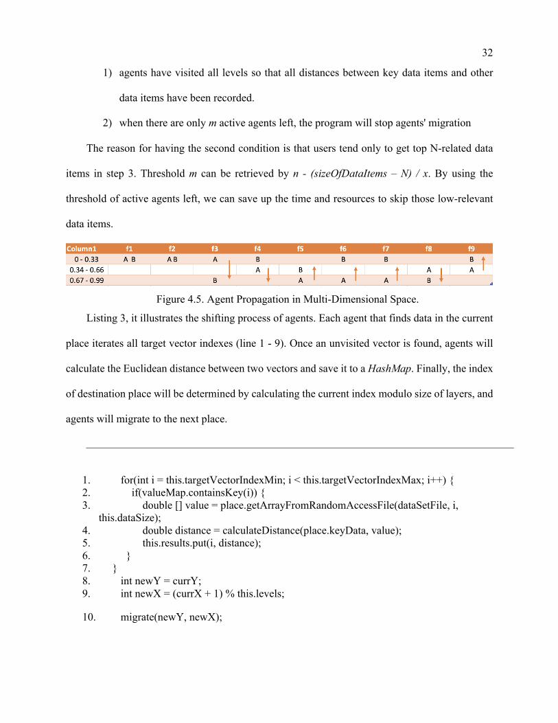
In this modified algorithm, we firstly evenly distribute the input data into multiple layers. For

instance, as illustrated in Figure 4.5, if the value of data items falls into the range from 0 to 1, and

we have three layers in total, each layer will be in the interval of 0 to 0.33, 0.34 to 0.66, and 0.67

to 1. Then we initialize 3 * n places in MASS where n is the dimension of the vector. During

agents’ initialization, agents migrate to the starting place where the key data item has valid data in

the corresponding column and agent level. Agents will traverse along the vertical direction to

discover if surrounding places contain the value of other data items. Upon arriving at a new place

that maintains a value between 0 and 1, the agent calculates the distance between the key data item

and corresponding data item and then saves the results in memory. To avoid duplicate distance

calculation, we assign each agent with a group of consecutive data items. The index of data item

can be determined from sizeOfDataItem/agentSize ∗ agentIndex to sizeOfDataItem/

agentSize ∗ (agentIndex + 1). This can also give us a number of data items that an agent is

responsible for (x). The migration will stop when the following conditions reached:

32

1) agents have visited all levels so that all distances between key data items and other

data items have been recorded.

2) when there are only m active agents left, the program will stop agents' migration

The reason for having the second condition is that users tend only to get top N-related data

items in step 3. Threshold m can be retrieved by n - (sizeOfDataItems – N) / x. By using the

threshold of active agents left, we can save up the time and resources to skip those low-relevant

data items.

Figure 4.5. Agent Propagation in Multi-Dimensional Space.

Listing 3, it illustrates the shifting process of agents. Each agent that finds data in the current

place iterates all target vector indexes (line 1 - 9). Once an unvisited vector is found, agents will

calculate the Euclidean distance between two vectors and save it to a HashMap. Finally, the index

of destination place will be determined by calculating the current index modulo size of layers, and

agents will migrate to the next place.

1. for(int i = this.targetVectorIndexMin; i < this.targetVectorIndexMax; i++) { 2. if(valueMap.containsKey(i)) { 3. double [] value = place.getArrayFromRandomAccessFile(dataSetFile, i,

this.dataSize); 4. double distance = calculateDistance(place.keyData, value); 5. this.results.put(i, distance); 6. } 7. } 8. int newY = currY; 9. int newX = (currX + 1) % this.levels;

10. migrate(newY, newX);

33

Listing 3. Distance Calculation and Agent Migration

4.4.2 File I/O with RandomAccessFile

In this implementation, the size of memory space limits the data that can be retrieved, 8GB

memory space can only fit 500,000 rows with 2000 features. In addition, in the real database

system, data is usually saved in the hard disk instead of memory space. Therefore, we decide to

bring RandomAccessFile for agents to retrieve values of data items.

A random access file behaves like a large array of bytes [24]. A file pointer, which is similar

to a cursor, can be moved to any position on the byte array. It reads bytes starting at the file pointer

and advances a certain number of bytes to read the content. Similar to previously mentioned

parallel I/O, this feature is also added to the place class.

By implementing these functions, MASS is able to access the data directly from the hard drive

instead of saving all of them into RAM. There are several tradeoffs of using this methodology.

First of all, MASS gets rid of the restrictions of memory space. Place doesn't need to keep a copy

of the whole database. Instead, agents can access their required records on demand. This behavior

simulates data querying in the real database. Technically, we can handle any size of database using

this methodology. Moreover, in MMM, users don't query all related data items under a semantic

space. Instead, only top N items will be returned. In this case, the number of file I/O can be limited.

While the frequency of file I/O is narrowed down, the speed of reading a file from a hard drive is

still much slower than directly taking it from memory space. If the number of file I/O gets bigger,

it will inevitably reduce efficiency.

34

Chapter 5. RESULTS

This chapter shows experimental results of MASS and MPI implementations discussed in

Chapter 3. It also compares the experimental results with sequential. The detailed benchmarks

data can be found in Appendix.

5.1 EXECUTION ENVIRONMENT

The experiments are conducted in cssmpi cluster at the University of Washington Bothell. There

are eight computing nodes in cssmpi cluster which provides us with 4-core Intel(R) Xeon(R)

Gold 6130 CPU with 20GB memory space. The MASS library 1.3.0 and MPI Java [25] are used

in our experiment. The MASS java is configured with 4GB initial heap size and 12GB maximum

heap space. The testing dataset is random generated with double precision.

5.2 MATRIX MULTIPLICATION

5.2.1 Computation Results

The experiments were conducted to evaluate and compare large-scale matrix multiplication

performance using MASS, MPI Java and sequential Java programs. Previous students have

conducted benchmark comparisons between MASS with Spark and MapReduce. The results

showed that Spark and MapReduce were much slower than MASS [26]. Therefore, we only

compare MASS with MPI Java in our benchmark.

For MASS and MPI Java, they use Cannon's algorithm, and the sequential Java program uses

the basic matrix multiplication algorithm. The testing data is a square matrix that has 2048 rows

and 2048 columns. We used four computing nodes to conduct benchmarks with both MPI and

MASS. The number of computing nodes must be divisible by the matrix size in Cannon’s

35

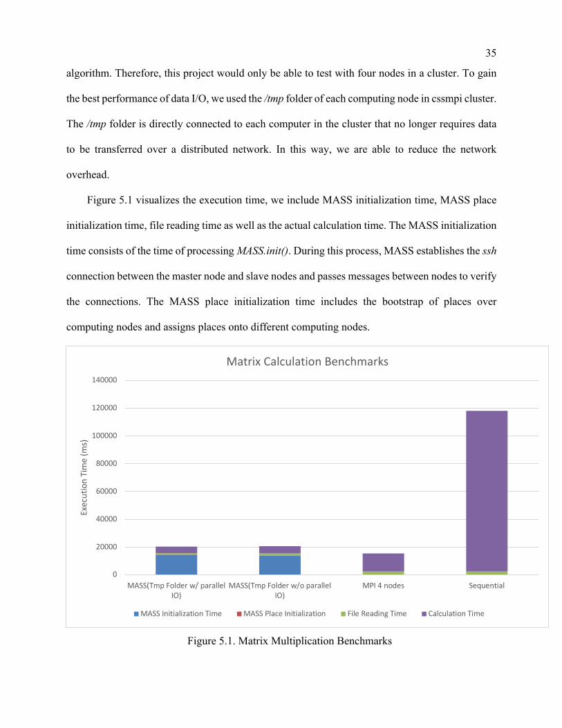
algorithm. Therefore, this project would only be able to test with four nodes in a cluster. To gain

the best performance of data I/O, we used the /tmp folder of each computing node in cssmpi cluster.

The /tmp folder is directly connected to each computer in the cluster that no longer requires data

to be transferred over a distributed network. In this way, we are able to reduce the network

overhead.

Figure 5.1 visualizes the execution time, we include MASS initialization time, MASS place

initialization time, file reading time as well as the actual calculation time. The MASS initialization

time consists of the time of processing MASS.init(). During this process, MASS establishes the ssh

connection between the master node and slave nodes and passes messages between nodes to verify

the connections. The MASS place initialization time includes the bootstrap of places over

computing nodes and assigns places onto different computing nodes.

Figure 5.1. Matrix Multiplication Benchmarks

0

20000

40000

60000

80000

100000

120000

140000

MASS(Tmp Folder w/ parallelIO)

MASS(Tmp Folder w/o parallelIO)

MPI 4 nodes Sequential

Exec

utio

n Ti

me

(ms)

Matrix Calculation Benchmarks

MASS Initialization Time MASS Place Initialization File Reading Time Calculation Time

36

MPI Java takes 15319.6 milliseconds in total, which exceeded MASS and sequential

program's performance. MASS also has good performance results, which achieves 20370.83

milliseconds using parallel I/O and 20587.67 milliseconds without using parallel I/O. When we

look at the calculation time only, MASS has the best performance. It takes around 5000

milliseconds while MPI Java takes 12937.2 milliseconds and the sequential program takes over

115693.8 milliseconds. By comparing the calculation performance between MASS and MPI, we

can see that MASS improves over 95% from the sequential program while MPI Java improves

around 88% from the sequential program. This is because MASS uses multi-core capability,

whereas MPI only uses a single core on each machine. In this case, the number of computing nodes

of MASS increases from 4 to 16, and each computing node is responsible for a smaller submatrix

size so that the overall performance is faster than MPI. In MASS, the MASS initialization time

takes the most time. This time is static, and it will not change with the change of the number of

computing nodes. In this case, we expect the percentage of MASS initialization will be relatively

small when we use more computing nodes, and MASS will have a chance to surpass MPI in terms

of overall performance.

In MPI Java programs, the file reading time is around 2300 milliseconds, accounting for 15%

of the overall processing time. MASS improves the file reading time significantly by implementing

the parallel I/O. It dropped the file reading time from 1507 milliseconds to 993 milliseconds which

is a 34% improvement.

5.2.2 MASS Programmability Analysis

This section discusses programmability analysis between MASS with MapReduce, Spark, and

MPI Java.

37

MapReduce and Spart introduce a new programming paradigm. With MapReduce, operations

are separated into two types of procedures, Map and Reduce. The map procedure filters and sorts

the input data, and the reduce method behaves like a summary operation [27]. The whole process

is very similar to the divide and conquer algorithm. This programming model with multi-threaded

implementations provides better scalability and fault tolerance. In order to fit the model of

MapReduce, developers need to be familiar with new data structures (Map and Queue), which will

bring extra learnings to developers.

Spark is a cluster computing platform, and it extends MapReduce to support nonlinear

dataflow structure on distributed programs [28]. The core of Spark is Resilient Distributed Dataset

(RDD), which is a read-only collection of items distributed across computing nodes in a cluster.

The input data is transformed into RDDs in a Spark application, and each computing node receives

a corresponding portion of RDD partitions. In Spark application, there are two types of operations.

Transformation converts the data input into a new RDD, and Action performs operations on input

RDD to return results. Same as the abovementioned MapReduce, this new programming paradigm

brings a steep learning curve to developers. Moreover, during the data stream, the data

transformation in MapReduce and Spark leads to extra unnecessary efforts to satisfy the

framework's requirements. This drawback in iterative MapReduce or RDD transformations results

in additional overhead due to the need to exchange data over clusters.

On the contrary, MASS uses an agent-based approach, and it simulates the problem-solving

process using agents. Although Spark has a built-in matrix multiplication library, RDD requires

transforming all input data instead of submatrix only. Since communication among data items is

only allowed from data shuffling and sorting in Spark and MapReduce, their implementation of

matrix multiplication is extremely difficult. On the other hand, a matrix is laid out smoothly over

38

a cluster system with places, and agents work as messengers in Cannon’s algorithm. That’s why

MASS can parallelize Cannon’s algorithm much easier than Spark and MapReduce.

When we look at Cannon’s algorithm with MASS and MPI Java, the most challenging part in

Cannon’s algorithm is data transmission between different ranks. In MPI, this can be achieved

using MPI_SEND and MPI_RECV. Since MPI doesn’t support multiple dimension array data

transmission, we have to allocate arrays into a contiguous format. Moreover, MPI ranks are

organized in linear order. Developers have to map their rank numbers into a 2d array to get the

relationship between rank number and submatrices' id. MPI provides users with MPI_Cart_create

method to create a communicator in a 2d topology format. We utilize this method to achieve rank

mapping. In contrast, MASS offers a more convenient way to work with Cannon's algorithm than

MPI Java. Places are a multidimensional array so that they can easily be mapped with submatrices.

MASS utilizes agents to carry data among computing nodes, and this gives developers a more

intuitive way to think about data transactions.

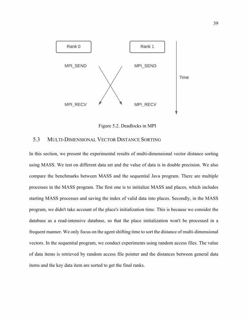
Lastly, the deadlock is the most common mistake in MPI. Developers have to be aware that

for every MPI_SEND there must be a pairing MPI_RECV. For example, as shown in Figure 5.2,

this may end in deadlock as rank 0 and rank 1 are sending simultaneously, but none of them are

receiving data. In comparison with MPI, MASS allows flexible communication between

submatrices that won't cause deadlock during data transmission. Thus, matrix multiplication

requiring frequent data transmission between submatrices benefit from MASS's flexibility and

reliability.

39

Figure 5.2. Deadlocks in MPI

5.3 MULTI-DIMENSIONAL VECTOR DISTANCE SORTING

In this section, we present the experimental results of multi-dimensional vector distance sorting

using MASS. We test on different data set and the value of data is in double precision. We also

compare the benchmarks between MASS and the sequential Java program. There are multiple

processes in the MASS program. The first one is to initialize MASS and places, which includes

starting MASS processes and saving the index of valid data into places. Secondly, in the MASS

program, we didn't take account of the place's initialization time. This is because we consider the

database as a read-intensive database, so that the place initialization won't be processed in a

frequent manner. We only focus on the agent shifting time to sort the distance of multi-dimensional

vectors. In the sequential program, we conduct experiments using random access files. The value

of data items is retrieved by random access file pointer and the distances between general data

items and the key data item are sorted to get the final ranks.

40

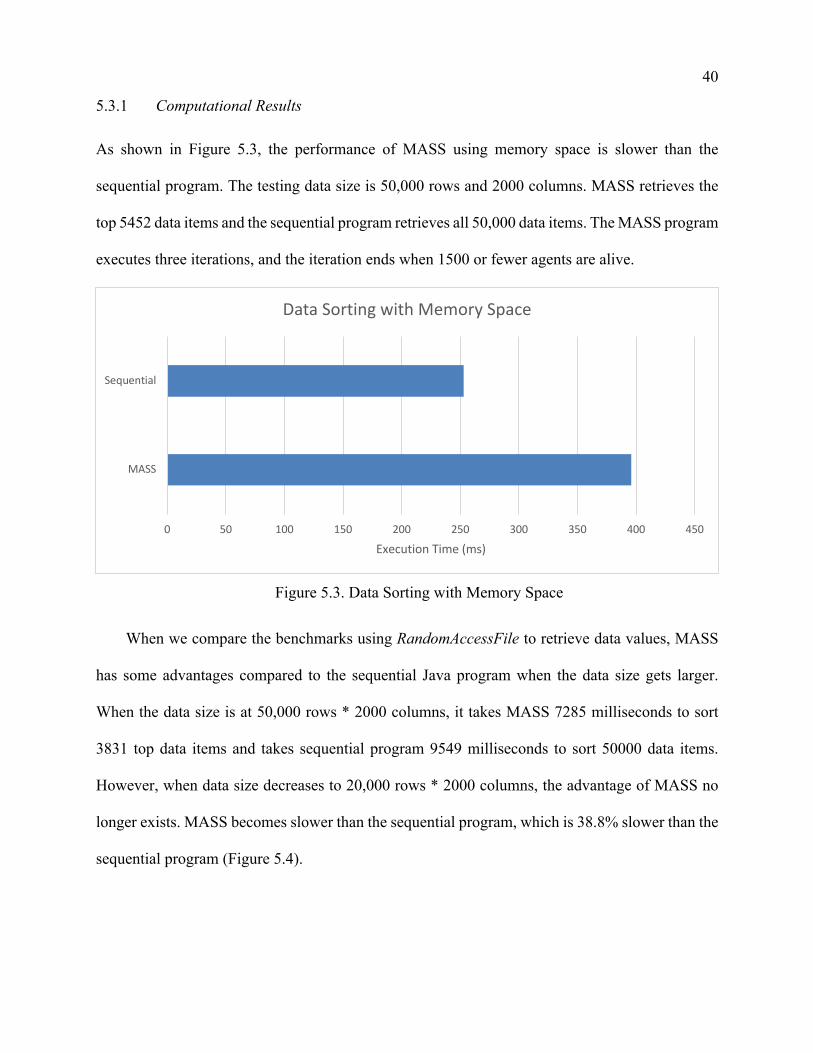
5.3.1 Computational Results

As shown in Figure 5.3, the performance of MASS using memory space is slower than the

sequential program. The testing data size is 50,000 rows and 2000 columns. MASS retrieves the

top 5452 data items and the sequential program retrieves all 50,000 data items. The MASS program

executes three iterations, and the iteration ends when 1500 or fewer agents are alive.

Figure 5.3. Data Sorting with Memory Space

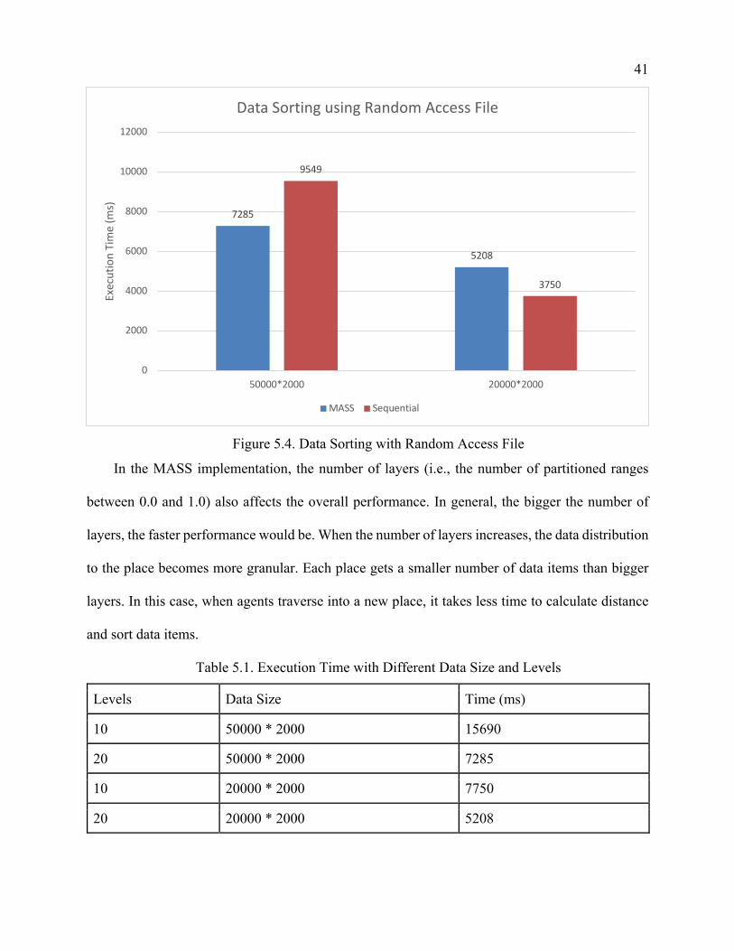
When we compare the benchmarks using RandomAccessFile to retrieve data values, MASS

has some advantages compared to the sequential Java program when the data size gets larger.

When the data size is at 50,000 rows * 2000 columns, it takes MASS 7285 milliseconds to sort

3831 top data items and takes sequential program 9549 milliseconds to sort 50000 data items.

However, when data size decreases to 20,000 rows * 2000 columns, the advantage of MASS no

longer exists. MASS becomes slower than the sequential program, which is 38.8% slower than the

sequential program (Figure 5.4).

0 50 100 150 200 250 300 350 400 450

MASS

Sequential

Execution Time (ms)

Data Sorting with Memory Space

41

Figure 5.4. Data Sorting with Random Access File

In the MASS implementation, the number of layers (i.e., the number of partitioned ranges

between 0.0 and 1.0) also affects the overall performance. In general, the bigger the number of

layers, the faster performance would be. When the number of layers increases, the data distribution

to the place becomes more granular. Each place gets a smaller number of data items than bigger

layers. In this case, when agents traverse into a new place, it takes less time to calculate distance

and sort data items.

Table 5.1. Execution Time with Different Data Size and Levels

Levels Data Size Time (ms)

10 50000 * 2000 15690

20 50000 * 2000 7285

10 20000 * 2000 7750

20 20000 * 2000 5208

7285

5208

9549

3750

0

2000

4000

6000

8000

10000

12000

50000*2000 20000*2000

Exec

utio

n Ti

me

(ms)

Data Sorting using Random Access File

MASS Sequential

42

Considering the scenarios in real-world database systems, MASS can be utilized to query

large-scale databases. Once MASS applications and places are initialized, the performance of data

querying is superior to the sequential Java program. In addition, MASS is also able to handle

multiple querying requests in parallel. Upon a new request arrives, a new group of agents could be

spawned onto places and migrate to the neighbors to fulfill the user's request. However, the

sequential program has to re-calculate the distance whenever the key data item got changed.

Additionally, when data size gets larger, MASS can easily pick up the most related data items

using the agent migration approach, while a sequential program needs to sort all data items that

put it in a disadvantaged position. Therefore, MASS is well suited for multi-dimensional vector

distance sorting in the data querying context.

Chapter 6. CONCLUSION

6.1 ACHIEVEMENT

As a database, MMM handles data queries on the fly in accordance with the user-provided

impression words. It applied semantic correlations computations between different data items with

context computation mechanisms. After examining the performance conducted by the sequential

program, we found MMM is a high computational framework that requires large-scale

mathematical operations. When the data size is 40,000 rows * 2000 columns, the total execution

time of MMM is over 40 minutes. MMM creates a space to save data items, and places of MASS

can support this space. Therefore, we applied MASS to parallelize MMM using the agent-based

methodology.

For step 1 of MMM, we utilized Cannon’s Algorithm with MASS. MASS showed a

significant performance improvement over the sequential program and MPI Java program. On

43

average, MASS with parallel I/O achieved 23 times speedup over the sequential program on 2048

* 2048 matrix multiplication. By comparison with other parallel frameworks, it also improved the

efficiency by 2.47 times over MPI Java. With the new parallel I/O feature added into MASS,

MASS utilized the advantage of distributed systems to reduce the overhead in data I/O. The file

reading time reduced by 57% compared to the sequential execution. This feature also enhanced

the scalability of MASS to deal with millions of data with a moderate performance

impact. Concluding that, MMM delivered the best computation performance with reactive agents

and facilitated user-defined submatrices mapping in distributed arrays.

The work of sorting distance of multidimensional vectors indicates that MASS is capable of

solving real-world problems. In comparison with the sequential problem, MASS provides a

solution for high concurrency scenarios. MASS is suitable to handle multiple requests concurrently

with multi-threading programming. Additionally, MASS also offers a competitive benchmark to

acquire the top related data items in MMM.

6.2 FUTURE WORK

As for future work, the following tasks can be implemented. In step 2 of MMM, the parallelization

of eigen decomposition is not finished. In the future, eigen decomposition can be parallelized along

with divide and conquer techniques to improve the performance significantly. In MMM, we want

to clarify some technical details of step 3. The projections between vectors to the semantic space

are still ambiguous. We want to identify the accurate math formulas to identify the projections

between vectors to the semantic space. Besides, in our implementations, we tried handling multiple

querying requests at the same time. However, we are not clear what the maximum limitations of

MASS are. Hence, we want to test the max number of concurrent requests that the system can

handle. Furthermore, MASS and MMM require a real-world database to verify correctness and

44

efficiency. This would give us more confidence in our integrated system to apply to more practical

applications in the future.

45

BIBLIOGRAPHY [1] Y. Kiyoki and X. Chen, "A Semantic Associative Computation Method for Automatic

Decorative-Multimedia Creation with 'Kansei' Information," p. 10.

[2] T. Kitagawa and Y. Kiyoki, "A mathematical model of meaning and its application to multidatabase systems," in Proceedings RIDE-IMS '93: Third International Workshop on Research Issues in Data Engineering: Interoperability in Multidatabase Systems, Vienna, Austria, 1993, pp. 130–135. doi: 10.1109/RIDE.1993.281933.

[3] M. Fukuda, C. Gordon, U. Mert, and M. Sell, "An Agent-Based Computational Framework for Distributed Data Analysis," Computer, vol. 53, no. 3, pp. 16–25, Mar. 2020, doi: 10.1109/MC.2019.2932964.

[4] J. Emau, T. Chuang, and M. Fukuda, "A multi-process library for multi-agent and spatial simulation," in Proceedings of 2011 IEEE Pacific Rim Conference on Communications, Computers and Signal Processing, Victoria, BC, Canada, Aug. 2011, pp. 369–375. doi: 10.1109/PACRIM.2011.6032921.

[5] C. Gordon, U. Mert, M. Sell, and M. Fukuda, "Implementation Techniques to Parallelize Agent-Based Graph Analysis," in Highlights of Practical Applications of Survivable Agents and Multi-Agent Systems. The PAAMS Collection, Cham, 2019, pp. 3–14. doi: 10.1007/978-3-030-24299-2_1.

[6] “Semantic Database: Concept, Architecture and Implementation," CodeProject, Oct. 25, 2014. https://www.codeproject.com/Articles/832959/Semantic-Database-Concept-Architecture-and-Impleme (accessed May 30, 2021).

[7] T. Chuang and M. Fukuda, "A Parallel Multi-agent Spatial Simulation Environment for Cluster Systems," in 2013 IEEE 16th International Conference on Computational Science and Engineering, Sydney, Australia, Dec. 2013, pp. 143–150. doi: 10.1109/CSE.2013.32.

[8] M. Sell and M. Fukuda, "Agent Programmability Enhancement for Rambling over a Scientific Dataset," in Advances in Practical Applications of Agents, Multi-Agent Systems, and Trustworthiness. The PAAMS Collection, vol. 12092, Y. Demazeau, T. Holvoet, J. M. Corchado, and S. Costantini, Eds. Cham: Springer International Publishing, 2020, pp. 251–263. doi: 10.1007/978-3-030-49778-1_20.

[9] A. S. Talwadker, "Survey of performance issues in parallel database systems," J. Comput. Sci. Coll., vol. 18, no. 6, pp. 5–9, Jun. 2003.

[10] F. Liu, L. Yin, and S. Blanas, "Design and Evaluation of an RDMA-aware Data Shuffling Operator for Parallel Database Systems," ACM Trans. Database Syst., vol. 44, no. 4, pp. 1–45, Dec. 2019, doi: 10.1145/3360900.

[11] E. Rahm, "Parallel query processing in shared disk database systems," SIGMOD Rec., vol. 22, no. 4, pp. 32–37, Dec. 1993, doi: 10.1145/166635.166649.

46

[12] M. Hammer and D. McLeod, "The semantic data model: a modelling mechanism for data base applications," in Proceedings of the 1978 ACM SIGMOD international conference on management of data - SIGMOD '78, Austin, Texas, 1978, p. 26. doi: 10.1145/509252.509264.

[13] "Semantic Web," Wikipedia. May 24, 2021. Accessed: May 30, 2021. [Online]. Available: https://en.wikipedia.org/w/index.php?title=Semantic_Web&oldid=1024772935

[14] A. M. Rinaldi and C. Russo, "A semantic-based model to represent multimedia big data," in Proceedings of the 10th International Conference on Management of Digital EcoSystems, Tokyo Japan, Sep. 2018, pp. 31–38. doi: 10.1145/3281375.3281386.

[15] V. Y. Pan and Z. Q. Chen, "The complexity of the matrix eigenproblem," in Proceedings of the thirty-first annual ACM symposium on Theory of computing - STOC '99, Atlanta, Georgia, United States, 1999, pp. 507–516. doi: 10.1145/301250.301389.

[16] H.-J. Lee, J. P. Robertson, and J. A. B. Fortes, "Generalized Cannon's algorithm for parallel matrix multiplication," in Proceedings of the 11th international conference on Supercomputing, New York, NY, USA, Jul. 1997, pp. 44–51. doi: 10.1145/263580.263591.

[17] "Cannon's algorithm for distributed matrix multiplication." https://iq.opengenus.org/cannon-algorithm-distributed-matrix-multiplication/ (accessed May 18, 2021).

[18] "MPI: A Message-Passing Interface Standard," p. 868.

[19] J. J. Dongarra and D. C. Sorensen, "On The Implementation Of A Fully Parallel Algorithm For The Symmetric Eigenvalue Problem,” San Diego, Apr. 1986, p. 45. doi: 10.1117/12.936874.

[20] “Symmetric Eigenproblems.” https://www.netlib.org/lapack/lug/node48.html (accessed May 18, 2021).

[21] “Tridiagonal matrix,” Wikipedia. Apr. 27, 2021. Accessed: May 18, 2021. [Online]. Available: https://en.wikipedia.org/w/index.php?title=Tridiagonal_matrix&oldid=1020127061

[22] "Householder transformation," Wikipedia. May 07, 2021. Accessed: May 18, 2021. [Online]. Available: https://en.wikipedia.org/w/index.php?title=Householder_transformation&oldid=1021914234

[23] J. J. Dongarra and D. C. Sorensen, "A Fully Parallel Algorithm for the Symmetric Eigenvalue Problem," SIAM J. Sci. and Stat. Comput., vol. 8, no. 2, pp. s139–s154, Mar. 1987, doi: 10.1137/0908018.

[24] "RandomAccessFile (Java Platform SE 7 )." https://docs.oracle.com/javase/7/docs/api/java/io/RandomAccessFile.html (accessed May 18, 2021).

47

[25] "MPI Java." https://www.open-mpi.org/faq/?category=java (accessed May 18, 2021).

[26] C. Liu, "Development of Application Programs Oriented to Agent-Based Data Analysis," p. 60.

[27] "MapReduce," Wikipedia. May 05, 2021. Accessed: Jun. 01, 2021. [Online]. Available: https://en.wikipedia.org/w/index.php?title=MapReduce&oldid=1021636888

[28] "Apache Spark," Wikipedia. Apr. 23, 2021. Accessed: Jun. 01, 2021. [Online]. Available: https://en.wikipedia.org/w/index.php?title=Apache_Spark&oldid=1019447044

48

APPENDIX A

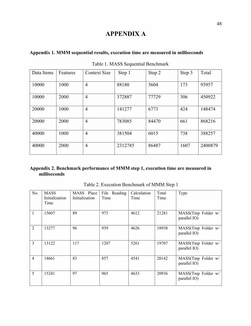
Appendix 1. MMM sequential results, execution time are measured in milliseconds

Table 1. MASS Sequential Benchmark

Data Items Features Context Size Step 1 Step 2 Step 3 Total

10000 1000 4 88180 5604 173 93957

10000 2000 4 372887 77729 306 450922

20000 1000 4 141277 6773 424 148474

20000 2000 4 783085 84470 661 868216

40000 1000 4 381504 6015 738 388257

40000 2000 4 2312785 86487 1607 2400879

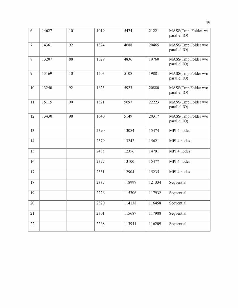
Appendix 2. Benchmark performance of MMM step 1, execution time are measured in milliseconds

Table 2. Execution Benchmark of MMM Step 1

No. MASS Initialization Time

MASS Place Initialization

File Reading Time

Calculation Time

Total Time

Type

1 15607 89 973 4612 21281 MASS(Tmp Folder w/ parallel IO)





49


7 14361 92 1324 4688 20465 MASS(Tmp Folder w/o parallel IO)






13

2390 13084 15474 MPI 4 nodes

14

2379 13242 15621 MPI 4 nodes

15

2435 12356 14791 MPI 4 nodes

16

2377 13100 15477 MPI 4 nodes

17 2331 12904 15235 MPI 4 nodes

18

2337 118997 121334 Sequential

19

2226 115706 117932 Sequential

20

2320 114138 116458 Sequential

21

2301 115687 117988 Sequential

22

2268 113941 116209 Sequential

50

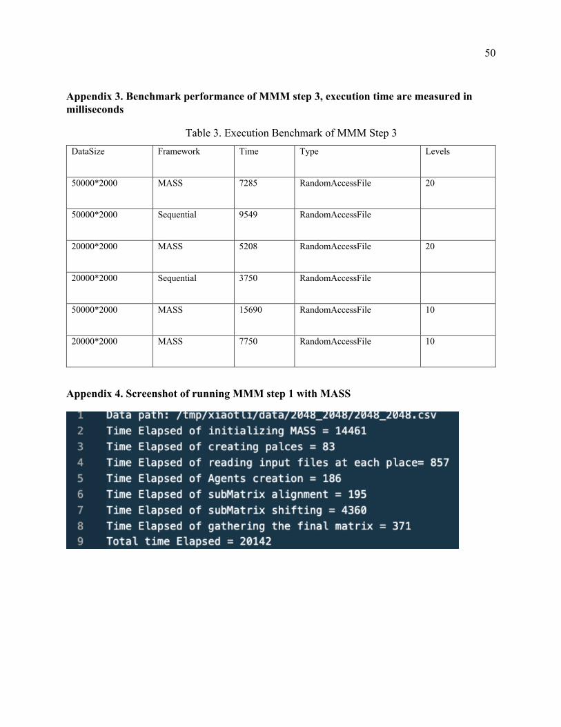
Appendix 3. Benchmark performance of MMM step 3, execution time are measured in milliseconds

Table 3. Execution Benchmark of MMM Step 3 DataSize Framework Time Type Levels

50000*2000 MASS 7285 RandomAccessFile 20

50000*2000 Sequential 9549 RandomAccessFile


20000*2000 Sequential 3750 RandomAccessFile



Appendix 4. Screenshot of running MMM step 1 with MASS

51

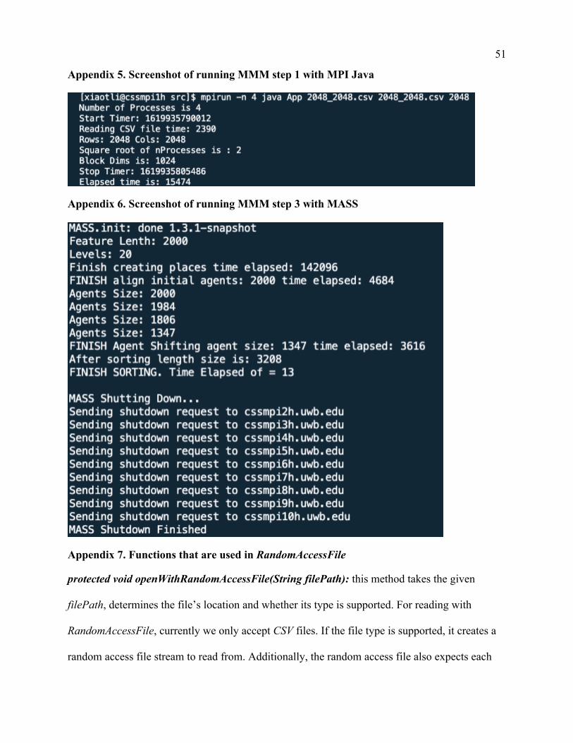
Appendix 5. Screenshot of running MMM step 1 with MPI Java

Appendix 6. Screenshot of running MMM step 3 with MASS

Appendix 7. Functions that are used in RandomAccessFile

protected void openWithRandomAccessFile(String filePath): this method takes the given

filePath, determines the file’s location and whether its type is supported. For reading with

RandomAccessFile, currently we only accept CSV files. If the file type is supported, it creates a

random access file stream to read from. Additionally, the random access file also expects each

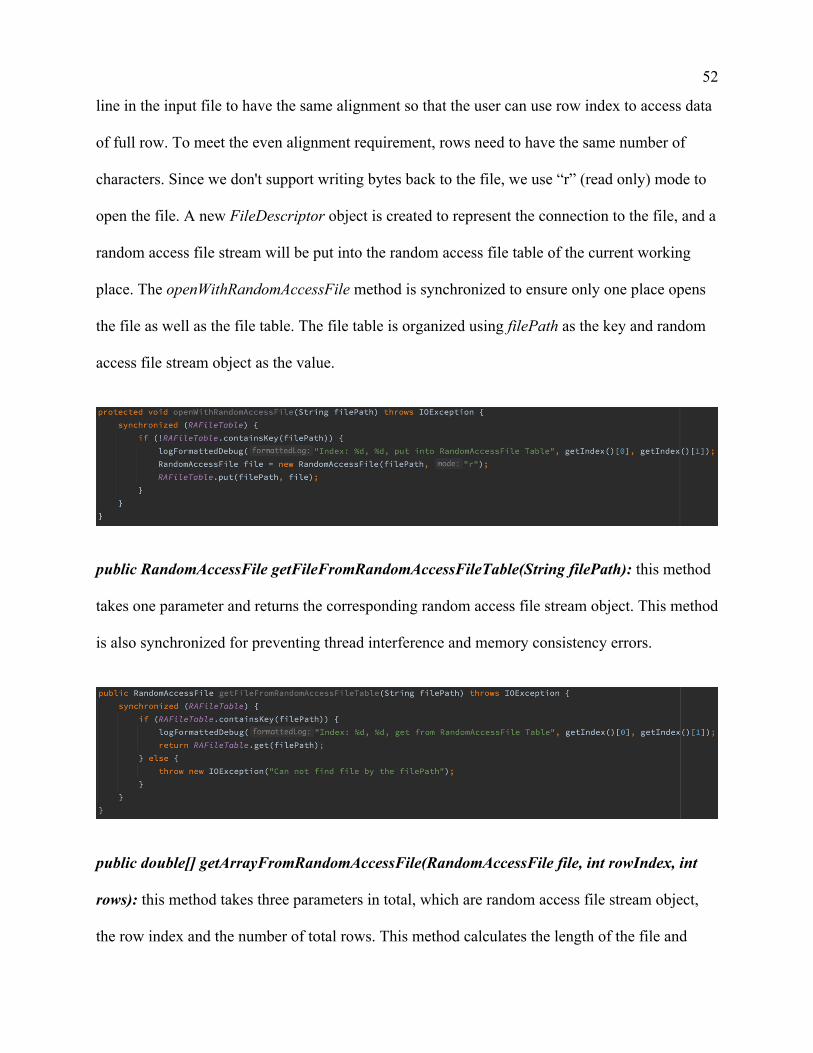
52

line in the input file to have the same alignment so that the user can use row index to access data

of full row. To meet the even alignment requirement, rows need to have the same number of

characters. Since we don't support writing bytes back to the file, we use “r” (read only) mode to

open the file. A new FileDescriptor object is created to represent the connection to the file, and a

random access file stream will be put into the random access file table of the current working

place. The openWithRandomAccessFile method is synchronized to ensure only one place opens

the file as well as the file table. The file table is organized using filePath as the key and random

access file stream object as the value.

public RandomAccessFile getFileFromRandomAccessFileTable(String filePath): this method

takes one parameter and returns the corresponding random access file stream object. This method

is also synchronized for preventing thread interference and memory consistency errors.

public double[] getArrayFromRandomAccessFile(RandomAccessFile file, int rowIndex, int

rows): this method takes three parameters in total, which are random access file stream object,

the row index and the number of total rows. This method calculates the length of the file and

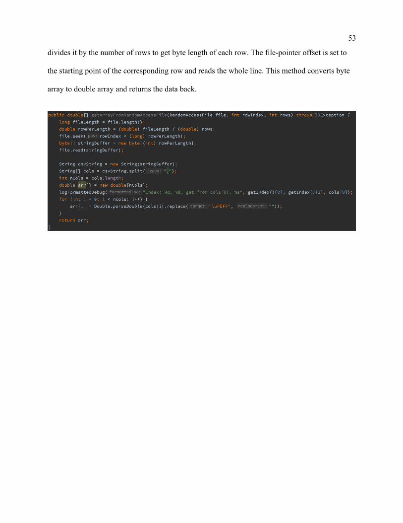
53

divides it by the number of rows to get byte length of each row. The file-pointer offset is set to

the starting point of the corresponding row and reads the whole line. This method converts byte

array to double array and returns the data back.

Documents

i © Copyright 2021 Xiaotian Li