Copyright by Xun Li 2018

Copyright

by

Xun Li

2018

The Dissertation Committee for Xun Li certifies that this is the approved version of the

following Dissertation:

OPPONENT MODELING AND EXPLOITATION IN POKER

USING EVOLVED RECURRENT NEURAL NETWORKS

Committee:

Risto Miikkulainen, Supervisor

Dana Ballard

Benito Fernandez

Aloysius Mok

OPPONENT MODELING AND EXPLOITATION IN POKER

USING EVOLVED RECURRENT NEURAL NETWORKS

by

Xun Li

Dissertation

Presented to the Faculty of the Graduate School of

The University of Texas at Austin

in Partial Fulfillment

of the Requirements

for the Degree of

Doctor of Philosophy


August 2018

To my mother, Rongsheng Li, my father, Weiru Guo, and my love, Yuanyuan Zhou,

for your support and patience.

v

Acknowledgements

I would like to start by thanking my research supervisor, Dr. Risto Miikkulainen,

for his invaluable guidance and support throughout my Ph.D. program. To me, he is not

only a knowledgeable mentor but also a great friend.

I would also like to thank my committee, Dr. Dana Ballard, Dr. Benito Fernandez,

and Dr. Aloysius Mok, for their suggestions and encouragement. Without their help, this

dissertation would not have been possible.

In addition, I would like to extend my appreciation to my friends and colleagues in

the Department of Computer Science at the University of Texas at Austin. It has been a

great honor and pleasure working in this lively and inspiring community.

Last but not least, I would like to thank my beloved family. In particular, I would

like to thank my Mom, who encouraged me to embark on my journey towards a Ph.D. It

would not be possible for this dream to come true without her love and dedication.

This research was supported in part by NIH grant R01- GM105042, and NSF grants

DBI-0939454 and IIS-0915038.

XUN LI


August 2018

vi

Abstract

Opponent Modeling and Exploitation in Poker

Using Evolved Recurrent Neural Networks

Xun Li, Ph.D.

The University of Texas at Austin, 2018

Supervisor: Risto Miikkulainen

As a classic example of imperfect information games, poker, in particular, Heads-

Up No-Limit Texas Holdem (HUNL), has been studied extensively in recent years. A

number of computer poker agents have been built with increasingly higher quality. While

agents based on approximated Nash equilibrium have been successful, they lack the ability

to exploit their opponents effectively. In addition, the performance of equilibrium strategies

cannot be guaranteed in games with more than two players and multiple Nash equilibria.

This dissertation focuses on devising an evolutionary method to discover opponent models

based on recurrent neural networks.

A series of computer poker agents called Adaptive System for Hold’Em (ASHE)

were evolved for HUNL. ASHE models the opponent explicitly using Pattern Recognition

Trees (PRTs) and LSTM estimators. The default and board-texture-based PRTs maintain

statistical data on the opponent strategies at different game states. The Opponent Action

Rate Estimator predicts the opponent’s moves, and the Hand Range Estimator evaluates

vii

the showdown value of ASHE’s hand. Recursive Utility Estimation is used to evaluate the

expected utility/reward for each available action.

Experimental results show that (1) ASHE exploits opponents with high to moderate

level of exploitability more effectively than Nash-equilibrium-based agents, and (2) ASHE

can defeat top-ranking equilibrium-based poker agents. Thus, the dissertation introduces

an effective new method to building high-performance computer agents for poker and other

imperfect information games. It also provides a promising direction for future research in

imperfect information games beyond the equilibrium-based approach.

viii

Table of Contents

List of Tables ................................................................................................................... xiii

List of Figures .................................................................................................................. xiv

Chapter 1: Introduction ........................................................................................................1

1.1. Motivation ............................................................................................................1

1.2. Challenge .............................................................................................................3

1.3. Approach ..............................................................................................................5

1.4. Guide to the Readers ............................................................................................7

Chapter 2: Heads-Up No-Limit Texas Holdem ...................................................................9

2.1. Rules of the Game................................................................................................9

2.2. Rankings of Hands in Texas Holdem ................................................................12

2.3. Related Terminology .........................................................................................16

Chapter 3: Related Work ...................................................................................................21

3.1. Computer Poker and Nash Equilibrium Approximation ...................................21

3.1.1. Simple Poker Variants ........................................................................22

3.1.2. Full-scale Poker ..................................................................................23

Equilibrium Approximation Techniques .............................................23

Abstraction Techniques .......................................................................25

3.1.3. Conclusions on Nash Equilibrium Approximation .............................26

3.2. Opponent Modeling and Exploitation................................................................27

3.2.1. Non-equilibrium-based Opponent Exploitation..................................27

Rule-based Statistical Models ..............................................................28

Bayesian Models ..................................................................................29

ix

Neural Networks ..................................................................................30

Miscellaneous Techniques ...................................................................31

3.2.2. Equilibrium-based Opponent Exploitation .........................................31

3.2.3. Conclusions on Opponent Modeling ..................................................34

3.3. LSTM and Neuroevolution ................................................................................34

3.3.1. LSTM Neural Networks .....................................................................35

3.3.2. Neuroevolution ...................................................................................37

3.3.3. Conclusions .........................................................................................40

Chapter 4: Evolving LSTM-based Opponent Models .......................................................41

4.1. ASHE 1.0 Architecture ......................................................................................41

4.1.1. LSTM Modules ...................................................................................43

4.1.2. Decision Network and Decision Algorithm........................................44

4.2. Method of Evolving Adaptive Agents ...............................................................45

4.2.1. Motivation ...........................................................................................45

4.2.2. Evolutionary Method ..........................................................................46

4.3. Experimental Results .........................................................................................48

4.3.1. Experimental Setup .............................................................................48

Training Opponents .............................................................................49

Evaluation and Selection......................................................................50

Parameter Settings ...............................................................................51

4.3.2. Adaptation, Exploitation, and Reliability ...........................................52

4.3.3. Slumbot Challenge ..............................................................................55

4.4. Discussion and Conclusion ................................................................................57

x

Chapter 5: Pattern Recognition Tree and Explicit Modeling.............................................59

5.1. ASHE 2.0 Architecture ......................................................................................59

5.1.1. Motivation and Framework ................................................................60

Motivation: Pattern Recognition Tree .................................................60

Motivation: Explicit Modeling and Utility-based Decision-making ...62

5.1.2. Opponent Model .................................................................................64

Pattern Recognition Tree .....................................................................64

LSTM Estimators .................................................................................68

5.1.3. Decision Algorithm.............................................................................71

5.2. Evolution of the LSTM Estimators ....................................................................72



5.3.2. Training and Testing Opponents.........................................................75

5.3.3. Results and Analysis ...........................................................................76

Performance vs. High-exploitability Opponents..................................78

Performance vs. Low-exploitability Opponents ..................................79

Performance vs. Dynamic Strategies ...................................................80

Training Opponent(s) and Performance...............................................83

5.4. Discussion and Conclusion ................................................................................85

Chapter 6: Advanced PRT .................................................................................................87

6.1. Default PRT .......................................................................................................87

6.1.1. Motivation ...........................................................................................87

6.1.2. Construction and Application .............................................................89

xi

Construction .........................................................................................89

Application ...........................................................................................91

6.2. Board-Texture-Based PRT ................................................................................91

6.2.1. Motivation ...........................................................................................92

6.2.2. Implementation ...................................................................................93

Board-texture-based PRT Structure .....................................................93

Board Texture Clusters ........................................................................94



6.3.2. Results and Analysis ...........................................................................97

Chapter 7: Recurrent Utility Estimation ............................................................................99

7.1. Recurrent Utility Estimation ..............................................................................99

7.2. ASHE 2.2 Architecture ....................................................................................102

7.3. Experimental Results .......................................................................................104

7.3.1. Experimental Setup ...........................................................................104

7.3.2. Results and Analysis .........................................................................105

Chapter 8: Hand Range Analysis .....................................................................................109

8.1. Hand Range Analysis.......................................................................................109

8.2. Hand Range Estimator and the ASHE 2.3 Architecture ..................................110

8.3. Experimental Results .......................................................................................112

8.3.1. Evolving ASHE 2.3 ..........................................................................113

8.3.2. Performance vs. Highly Exploitable Opponents...............................113

8.3.3. Tournament Evaluation.....................................................................115

xii

Chapter 9: Discussion and Future Work ..........................................................................118

9.1. Training and Evaluation...................................................................................118

9.2. Reinforcement Learning ..................................................................................119

9.3. Generalization ..................................................................................................120

Chapter 10: Contributions and Conclusion ......................................................................122

10.1. Contributions .................................................................................................122

10.2. Conclusion .....................................................................................................124

References ........................................................................................................................126

xiii

List of Tables

Table 4-1: ASHE 1.0 Parameter Settings ..........................................................................52

Table 4-2: Opponent Exploitation .....................................................................................53

Table 4-3: Champion Action Statistics vs. Different Opponents ......................................54

Table 5-1: Estimator Inputs ...............................................................................................69

Table 5-2: ASHE 2.0 Parameters .......................................................................................75

Table 5-3: Training and Testing Opponents ......................................................................76

Table 5-4: ASHE 2.0 Evaluation Results ..........................................................................77

Table 5-5: ASHE 2.0 and ASHE 1.0 vs. Low-Exploitability Opponents ..........................79

Table 5-6: Performance against Dynamic Strategies .........................................................81

Table 5-7: Snapshot Strategy Analysis ..............................................................................82

Table 6-1: Board Textures .................................................................................................95

Table 6-2: ASHE 2.1 Evaluation Results ..........................................................................97

Table 7-1: ASHE 2.2 Parameters. ....................................................................................105

Table 7-2: ASHE 2.2 Evaluation Results ........................................................................106

Table 8-1: ASHE 2.3 Parameters. ....................................................................................113

Table 8-2: ASHE Systems v. Highly Exploitable Opponents. ........................................114

Table 8-3: Tournament Evaluation Results .....................................................................116

xiv

List of Figures

Figure 2-1: A Standard Poker Deck ...................................................................................13

Figure 3-1: A Vanilla LSTM Block ...................................................................................36

Figure 3-2: Genetic Algorithm Framework .......................................................................38

Figure 4-1: ASHE 1.0 Architecture ...................................................................................42

Figure 4-2: ASHE 1.0 Decision Algorithm. ......................................................................44

Figure 4-3: ASHE 1.0 Training Opponents .......................................................................49

Figure 4-4: Champion Performance vs. Rule-based Players .............................................53

Figure 5-1: ASHE 2.0 Architecture ...................................................................................61

Figure 5-2: A Pattern Recognition Tree.............................................................................65

Figure 5-3: An LSTM Estimator........................................................................................68

Figure 5-4: Decision Algorithm (ASHE 2.0) .....................................................................71

Figure 6-1: ASHE with Default PRTs (ASHE 2.1) ...........................................................90

Figure 6-2: A Board-Texture-Base PRT ............................................................................94

Figure 7-1: Recurrent Utility Estimation .........................................................................100

Figure 7-2: ASHE with Recursive Utility Estimation (ASHE 2.2) .................................102

Figure 7-3: Sample Game – ASHE 2.2 v. Slumbot 2017 ................................................107

Figure 8-1: ASHE 2.3 Architecture .................................................................................112

1

Chapter 1: Introduction

Imagine a world where computers are not only tools we use but also colleagues and

collaborators with which we solve problems. For instance, you may be concerned about

how to protect the safety of your community, or wish to have the upper hand in an important

business negotiation, or simply hope to impress your friends in the next poker party. Many

such challenges entail hidden secrets and cunning opponents, and it would be nice to have

a loyal and intelligent computer partner on our side. Our tireless collaborators will help us

identify weaknesses, hone our skills, and devise our strategies whenever and wherever we

need. Such collaborators need to deal with imperfect information and deceptive opponents,

and they must be able to exploit opponent strategies through adaptation. This dissertation

is a step towards that goal.

1.1. MOTIVATION

Imperfect information games are an important AI problem with numerous real-

world applications, including cyber security, trading, business transaction and negotiation,

military decision-making, table games, etc.

Computer agents in imperfect information games must address two challenges.

First, the agents are unable to fully observe the state of the game. Second, opponents may

attempt to mislead the agents with deceptive actions. As an example, poker agents cannot

observe their opponents’ cards when making their moves (partial observation), and the

opponents may slow-play a strong hand or bluff (deception).

Game theoretic analysis have been the most common approach to solve these

problems. For instance, Sajjan et al. [2014] proposed a holistic cyber security approach in

which the interaction between the attacks and the defense mechanisms was modeled as an

2

imperfect information game. A game theory inspired defense architecture was developed

to defend against dynamic adversary strategies.

Vatsa et al. [2005] modeled the conflicting motives between an attacker and a credit

card fraud detection system as a multi-stage imperfect information game and proposed a

fraud detection system based on a game-theoretic approach.

Business transaction and negotiation can be modeled as imperfect information

games as well. For example, Cai and Wurman [2005] developed an agent that constructs a

bidding policy in sealed-bid auction by sampling the valuation space of the opponents,

solving corresponding complete information game, and aggregating the samples.

Wang and Wellman [2017] proposed an agent-based model of manipulating prices

in the financial markets through spoofing. Empirical game-theoretic analysis showed that

spoofing can be profitable in a market with heuristic belief learning traders. However, after

re-equilibrating games with spoofing, such manipulation hurts market surplus and reduces

the proportion of HBL traders.

As a classic imperfect information game, poker has been studied extensively in

recent years. It is an ideal problem for the research on imperfect information games for the

following reasons. First, most real world applications must be modeled as a formal game.

This process is domain-specific and can be quite challenging. Moreover, a problem can be

modeled in different ways, making it difficult to compare results. In contrast, poker games

are already well-defined formal games. Hence, there is no need to model and formalize the

problem. Experimental results are comparable for each variant of the game, and the

techniques can be generalized to formal games derived from other problem domains.

Second, simple variants of poker is manually solvable, while complex variants such

as No-limit Holdem can be extremely challenging. Therefore, poker games have been used

as the target problem for both early and recent studies.

3

Third, poker is one of the most popular games. Poker variants, e.g. Texas Holdem,

Omaha, etc., are enjoyed by millions of players all over the world. Thus, research on poker

is both fun and rewarding.

Existing work on poker focuses on two aspects: (1) equilibrium approximation and

(2) opponent modeling. Equilibrium approximation techniques are designed to minimum

exploitability, and opponent modeling techniques allow the agents to adapt to and exploit

the opponents for higher utility.

This dissertation addresses opponent modeling problem from a new perspective. It

applies genetic algorithms to evolve RNN-based adaptive agents for HUNL, providing an

effective new approach to building high-performance computer agents for poker and other

large-scale imperfect information games.

1.2. CHALLENGE

Equilibrium-approximation techniques, e.g. Counterfactual Regret Minimization

(CFR) have been applied to multiple variants of the game and have achieved remarkable

successes [Zinkevinch et al., 2007]. In particular, Heads-Up Limit Texas Holdem has been

weakly solved [Bowling et al., 2015]. Many powerful poker agents for Heads-Up No-Limit

Holdem (HUNL) have been built through CFR in combination with various abstraction

and/or sampling techniques [Gilpin and Sandholm, 2008a; Brown et al., 2015; Jackson,

2017]. In recent Human vs. AI competitions, Nash-equilibrium-based poker agents have

defeated top professional human players in HUNL with statistically significant margins

[Moravcik et al., 2017; Brown and Sandholm, 2017].

However, equilibrium-approximation approaches have three limitations. First, for

imperfect information games with a large state space, the quality of Nash-equilibrium

approximation can be far from ideal. While a real Nash-equilibrium strategy in a two-

4

player zero-sum game such as HUNL is theoretically unexploitable (i.e. the game value of

the best counter-strategy is zero), most top-ranking poker agents based on approximated

Nash equilibrium strategies are exploitable with a simple local best response method [Lisy

and Bowling, 2016].

Second, in imperfect information games with more than two players and multiple

equilibria, if the opponents are not following the same equilibrium as approximated by an

equilibrium-based agent, the agent’s performance cannot be guaranteed [Ganzfried, 2016].

Therefore, it is difficult to apply equilibrium-approximation approaches to many imperfect

information games with three or more players, such as poker tournaments, multi-party

business negotiation, and security resource allocation.

Third, unexploitability does not guarantee maximum utility. In most real-world

applications, the ultimate goal is not to become unexploitable but to achieve maximum

utility against any opponent. In the case of poker, the goal is to win as many chips as

possible. While a real equilibrium strategy is guaranteed not to lose money statistically to

any opponent, it is unlikely to be the most profitable strategy.

The most effective counter-strategy against each opponent is different, and only

through opponent modeling and adaptation, can a player approximate such counter-

strategies for all opponents. Therefore, opponent modeling and adaptation may be the next

step towards building stronger poker agents beyond Nash equilibrium approximation [Li

and Miikkulainen, 2017].

Existing work on opponent modeling lays a foundation for building high-quality

adaptive poker agents. A number of computer agents capable of exploiting weak opponents

have been built over the past two decades. However, few of them can achieve comparable

performance playing against cutting-edge equilibrium-based agents in large-scale games

such as HUNL (see Chapter 3 for details).

5

In recent years, researchers attempted to build adaptive poker agents by adjusting

precomputed equilibrium strategies according to opponent’s action frequencies [Ganzfried

and Sandholm, 2011 and 2015]. This approach reduces the exploitability of adaptive

agents, thereby allowing them to perform better against other equilibrium-based opponents.

Nevertheless, it only allows limited deviation from the Nash equilibrium strategy, thus

reducing the effectiveness of opponent exploitation.

This dissertation aims at developing a method to build adaptive poker agents with

recurrent-neural-network-based opponent models for HUNL. The goal of the research is to

build agents that are effective in modeling a wide range of opponents and exploiting their

weaknesses. In addition, they should achieve overall equivalent or better performance

playing against cutting-edge equilibrium-based opponents. Such approach does not

approximate equilibrium strategies and should be able to generalize to games with multiple

players and equilibria.

1.3. APPROACH

This dissertation proposes an evolutionary method to discover opponent models

based on recurrent neural networks. These models are combined with a decision-making

algorithm to build agents that can exploit their opponents through adaptation.

In HUNL, opponent strategies are not known but must be learned from gameplay.

While supervised learning is commonly adopted for training neural network models, the

lack of sufficient labeled training data makes it rather difficult to apply such techniques for

opponent modeling. In fact, even the best human players cannot agree on the probability

for the opponent taking different actions given the current game state and the entire history

of games played against that opponent.

6

A particular powerful approach for such domains is evolutionary computation: in

many comparisons with reinforcement learning, it has achieved better performance in

discovering effective strategies from gameplay [Stanley et al., 2005; Li and Miikkulainen,

2018]. Evolution evaluates the agents based on their fitness, i.e. the overall performance

against different opponents rather than specific predictions, thus requiring no labeled

training data.

To evaluate the proposed approach, a series of poker agents called Adaptive System

for Hold’Em (ASHE) were evolved for HUNL. ASHE models the opponent using Pattern

Recognition Trees (PRTs) and LSTM estimators.

The PRTs store and maintain statistical data on the opponent’s strategy. They are

introduced to capture exploitable patterns based on different game states, thus improving

performance against strong opponents. They can also reduce the complexity of the LSTM

modules, making evolution more efficient. There are two types of PRTs in ASHE: the

default PRTs and the regular PRTs. The default PRTs are fixed and serve as a background

model. They allow the agent to make effective moves when facing a new opponent or an

infrequent game state. The regular PRTs are reset and updated for each opponent. As more

games are played with the opponent, the regular PRTs data becomes increasingly reliable,

allowing the agent to capture exploitable patterns in the opponent strategy.

The LSTM estimators are recurrent neural network modules, which are optimized

through evolution. They receive sequential inputs derived from the game states and the

corresponding PRT data. The Opponent Action Rate Estimator predicts the probability of

different opponent actions. The Hand Range Estimator evaluates strength of the opponent’s

hand, allowing the agent to compute showdown value more accurately.

7

Decisions are made via Recursive Utility Estimation. The utility of each available

action is computed using the predictions from the LSTM estimators. Action utilities are

evaluated by aggregating possible future moves and corresponding results.

The above techniques are introduced separately in ASHE 1.0 through ASHE 2.3,

each technique improves ASHE’s performance substantially, leading to a system that can

defeat top-ranking Nash-equilibrium-based agents and outperform them significantly when

playing against weaker opponents.

1.4. GUIDE TO THE READERS

This dissertation is organized as follows:

Chapter 2 introduces the problem domain, i.e. Heads-Up No Limit Texas Holdem.

It specifies the rules of the game and rankings of the hands. It also defines common poker

terminology that is used in this dissertation.

Chapter 3 outlines related work on computer poker, including the state-of-the-art

approach of Nash Equilibrium Approximation, and existing work on opponent modeling

and exploitation in poker. It also presents the technical foundation of ASHE, including

recurrent neural networks and neuroevolution.

Chapter 4 introduces ASHE 1.0, a two-module LSTM-based agent evolved by

playing against highly exploitable opponents. ASHE 1.0 validates the methodology and

establishes a framework for evolving adaptive poker agents.

Chapter 5 presents ASHE 2.0, which employs Pattern Recognition Trees (PRTs) to

models the opponent explicitly. Experimental results in this chapter show that the system

is significantly more effective in exploiting weak opponents than equilibrium-based agents

and that it achieves comparable performance in matches against top-ranking poker agents.

8

Chapter 6 introduces ASHE 2.1 and advanced PRTs, which is capable of modeling

and exploiting patterns in opponent strategies that are related to board texture.

Chapter 7 introduces ASHE 2.2 and Recursive Utility Estimation. This technique

provides more accurate evaluation of action utilities, thus allowing the adaptive agent to

apply advanced poker tactics effectively.

Chapter 8 introduces ASHE 2.3 and Hand Range Estimator (HRE), which improves

showdown value estimation through range analysis. ASHE 2.3 outperforms top-ranking

equilibrium-based agents by a significant margin and is highly effective against opponents

with different level of exploitability.

Chapter 9 discusses the experimental results and points out potential directions for

future work, including using stronger training opponents, reinforcement learning, and

generalization to other imperfect information games.

Chapter 10 reviews the contributions of this dissertation and summarizes the

conclusions from it.

9

Chapter 2: Heads-Up No-Limit Texas Holdem

Texas Holdem is a popular variation of the card game of poker. No-Limit Texas

Holdem is regarded as one of the most challenging problems among imperfect information

games because of its enormous state space considering all possible combinations of hole

cards, community cards, and action sequences.

As an example, Heads-Up No-Limit Holdem in the format adopted by the Annual

Computer Poker Competition in recent years has approximately 6.31 × 10164 game states

and 6.37 × 10161 observable states [Johanson, 2013]. On the other hand, unlike most real

world applications, actions, states, and utilities (rewards) in Texas Holdem are clearly

defined by the rules of the game, making it easy to model the game mathematically.

Therefore, No-Limit Texas Holdem has become a classic problem in the research of

imperfect information games.

This dissertation, like most current researches on No-Limit Texas Holdem, focuses

on the two-player version of the game, i.e. Heads-Up No-Limit Holdem (HUNL). The rest

of this chapter presents the rules of the game and defines most poker terminology used in

this dissertation.

2.1. RULES OF THE GAME

In HUNL, two players compete for money or chips contributed by both of them,

i.e. the pot. At the beginning of each game, both players are forced to post a bet into the

pot, i.e. the blinds. One of the players posts a smaller bet called the Small Blind, the other

posts a bigger bet called the Big Blind. Usually, the big blind is twice the small blind, and

a “$50/$100 game” means a game with $50 small blind and $100 big blind.

Depending on the context, the term “Small Blind” and “Big Blind” may refer to the

player posting the corresponding forced bet. In HUNL, the Small Blind (player) can be

10

referred to as the “button” or the “dealer”. In a game session with multiple games, the

players play as the dealer and the Big Blind alternately.

At the beginning of a game, each player is dealt two cards, i.e. the hole cards, from

a standard 52-card poker deck. The hole cards are private to the receiver, thus making the

states of the game partially observable. The game is divided into four betting rounds:

preflop, flop, turn, and river. The players acts alternately in each betting rounds. The dealer

acts first preflop, and the big blind acts first in all other betting rounds. Players must choose

one of the following actions when it is their turn to act:

Raise: To raise is to commit more chips than the opponent. A raise not only

makes the pot bigger but also challenges the opponent to match the raise

by calling, (re-)raising, or moving all-in.

Call: To call is to match the opponent’s contribution to the pot. If the two

players have already committed the same amount of money to the pot

(i.e. the player does not need to commit more chips to match the

opponent’s contribution), the action is usually called “check”.

All-in: To go all-in is to commit all chips into the pot. An all-in may or may

not be a legitimate call or raise. In particular, if a player cannot afford

to call after the opponent raises or moves all-in, the player may go all-

in in response.

Fold: To fold is to concede the pot to the opponent. It is the only way for a

player to avoid committing more chips to the pot after a raise from the

opponent.

By convention, the size of a raise refers to the difference between chips committed

by the raiser after the raise and the chips committed by the opponent. If the opponent has

11

not raised in the current betting round, this action is usually called a “bet” or an “open

raise”. The minimum size of an open raise is equal to the Big Blind. If the opponent raised

in the current betting round, the minimum size of a raise is the size of the opponent’s last

raise.

If a player folds, the game ends, and the opponent wins the pot. Otherwise, the

betting round continues until both players have taken at least one action and committed the

same amount of chips into the pot.

As the game proceeds, five cards are dealt face up on the table. Each of them is a

community card, and the set of community cards is called the board. Specifically, the board

is empty preflop; three community cards are dealt at the beginning of the flop, a fourth

community card is dealt at the beginning of the turn, and the last community card is dealt

at the beginning of the river. The board is observable to both players throughout the game.

If neither player has folded by the end of the river, the game goes into a showdown.

In addition, at any point of the game, if a player who has moved all-in contributes no more

chips to the pot than the other, the game also goes into a showdown. In this case, unfinished

betting rounds are skipped, and the board is completed immediately.

Note that if the players have contributed different amount of chips into the pot, the

effective size of the pot is twice the amount committed by the player with less contribution.

Any additional chips are returned to the player with more contribution.

In a showdown, each player combines the hole cards with the board and chooses

five out of the seven cards (two hole cards plus five community cards) to form the best

possible hand. The player with the better hand wins the pot. If the two hands are equally

strong, the players split the pot. The next section presents the rankings of poker hands.

Thus, a player may win the pot in two ways: (1) forcing the opponent to fold before

showdown, or (2) going into a showdown with a stronger hand. In principle, a player should

12

choose actions based on their expected utilities in both aspects. The expected utilities of an

action can be estimated based on a player’s hole cards, the board, and the sequence of

actions in the game. Furthermore, since an HUNL game session usually contains hundreds

of games, the strategy of the opponent can be modeled and weaknesses exploited based on

the history of previous games.

The huge number of possible game states and clear mathematical definition of

HUNL make it one of the most challenging and interesting problems for research on

building high-performance computer agents for large-scale imperfect information games.

2.2. RANKINGS OF HANDS IN TEXAS HOLDEM

In a showdown, the winner is the player with a better five-card hand according to

the rankings of hands. There are nine categories of hands in Texas Holdem. The categories

are ranked based on the rarity of the hands. A hand in a higher-ranking category beats any

hand in a lower-ranking category. Hands in the same category are ranked relative to each

other by comparing the ranks of their respective cards.

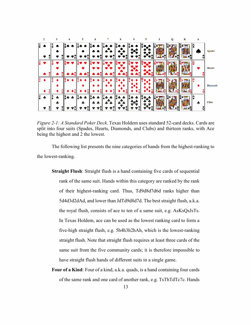
Texas holdem uses standard 52-card poker deck, which contains four suits, i.e.

Spades, Hearts, Diamonds, and Clubs. Each card has a rank. The ranks are: Ace (A), King

(K), Queen (Q), Jack (J), 10 (T), 9, 8, 7, 6, 5, 4, 3, 2, with Ace being the highest and 2 the

lowest. The suit of the cards do not affect their value in making a hand, e.g. Ace of Spades

is the same as Ace of Clubs.

For convenience of reference, cards in the rest of this dissertation are represented

by two-character strings where the first character represents the rank of the card, and the

second character represents the suit of the card. For example, “Ks” refers to king of spades,

“Th” Ten of Hearts, “5d” Five of Diamonds, and “2c” Two (a.k.a. Deuce) of Clubs.

13

Figure 2-1: A Standard Poker Deck. Texas Holdem uses standard 52-card decks. Cards are

split into four suits (Spades, Hearts, Diamonds, and Clubs) and thirteen ranks, with Ace

being the highest and 2 the lowest.

The following list presents the nine categories of hands from the highest-ranking to

the lowest-ranking.

Straight Flush: Straight flush is a hand containing five cards of sequential

rank of the same suit. Hands within this category are ranked by the rank

of their highest-ranking card. Thus, Td9d8d7d6d ranks higher than

5d4d3d2dAd, and lower than JdTd9d8d7d. The best straight flush, a.k.a.

the royal flush, consists of ace to ten of a same suit, e.g. AsKsQsJsTs.

In Texas Holdem, ace can be used as the lowest ranking card to form a

five-high straight flush, e.g. 5h4h3h2hAh, which is the lowest-ranking

straight flush. Note that straight flush requires at least three cards of the

same suit from the five community cards; it is therefore impossible to

have straight flush hands of different suits in a single game.

Four of a Kind: Four of a kind, a.k.a. quads, is a hand containing four cards

of the same rank and one card of another rank, e.g. TsThTdTc7c. Hands

14

in this category are ranked first by the rank of their quadruplet, and then

by the rank of the single card, i.e. the kicker. Thus, QsQhQdQcKh ranks

the same as QsQhQdQcKc, higher than 2s2h2d2cAs, and lower

thanAsAhAdAc7d.

Full House: Full house, a.k.a. boat, is a hand containing three cards of the

same rank and two cards (a pair) of another rank, e.g. KsKhKc2s2c.

Hands within this category are ranked first by the rank of the triplet, and

then by the rank of the pair. Therefore, 8s8h8d3h3c ranks the same

as8s8h8c3h3d, higher than 3s3h3c8s8h, and lower than AsAhAc2s2c.

Flush: Flush is a hand containing five cards of the same suit, not all of

sequential rank. Flush hands are ranked first by the rank of their highest-

ranking card, then by the second highest-ranking card, and so forth. For

example, AsJs8s5s2s ranks higher than KsQsJs8s5s, AsTs9s5s2s, or

AsJs8s4s3s, and lower than AsJs8s5s3s. Flush hands tie only if the

players are playing the board, i.e. the community cards form a flush,

which cannot be improved by the hole cards from any player. It is not

possible to have flush hands of different suits in a single game.

Straight: Straight is a hand containing five cards of sequential rank, not of

the same suit. Similar to straight flush, straights are ranked by the rank

of their highest-ranking card, regardless of the suit. Thus, Ts9c8h7d6c

ranks the same as Th9c8h7d6h, higher than 8h7d6c5d4d, and lower than

QhJdTs9c8h. The best possible straight, a.k.a. the Broadway, consists

of ace to ten of two or more suits, e.g. AsKsQhJhTc. The lowest-ranking

straight, a.k.a. the wheel, consists of five to ace of two or more suits,

e.g. 5d4c3s2hAd.

15

Three of a Kind: Three of a kind is a hand containing three cards of the

same rank and two cards from two other ranks. Hands within this

category are ranked first by their triplet, then by the rank of the higher-

ranking kicker, and finally by the lower-ranking kicker. For example,

JsJdJcTs8c ranks the same as JsJhJdTh8c, higher than TsThTdsAsJs,

and lower than JsJdJcAs2c or JsJdJcTs9h.

Two Pair: Two pair is a hand containing two cards of the same rank, two

cards of another rank, and one card from a third rank. Two pair hands

are compared first by the rank of the higher-ranking pair, then by the

rank of the lower-ranking pair, and finally by the kicker. For example,

AsAcTsTcQh is ranked higher than KhKdQsQhAs, and lower than

AsAhQhQcTc or AsAhTsTcKc.

One Pair: One pair is a hand containing two cards of the same rank and

three cards of three other ranks. Hands in this category are ranked first

by the rank of the pair, then by the rank of the kickers from highest to

the lowest. Therefore, AsAcKhTc7h ranks higher than KsKhAsTc7h,

AsAcQsJdTc or AsAcKhTc2d.

High Card: High card, a.k.a. no-pair or nothing, is a hand containing five

cards not all of sequential rank or of the same suit, and none of which

are of the same rank. Hands in this category are ranked first by their

highest-ranking card, then the second-highest-ranking card, and so

forth. Thus, AsJh8s5d2s ranks higher than KcQsJh8s5d, AsTs9h5d2s,

or AsJh8s4d3c, and lower than AsJh8s5d3s.

16

The game rules in the previous section and the above rankings of hands define the

imperfect information game studied in this dissertation.

2.3. RELATED TERMINOLOGY

This section introduces some common poker terms used in this dissertation.

Bluff and Semi-bluff: A bluff is a raise (bet) or all-in for the purpose of

inducing a fold from the opponent. Usually, the bluffer is holding a hand

that is (believed to be) unlikely to win in a showdown. In a semi-bluff,

while the bluffer’s hand is unlikely to win at the time of the bluff, it is

possible to be improved by community cards dealt in future betting

rounds (thus becoming the winning hand in a showdown).

As an example, suppose a player holds Qs7s, and the board contains

AsTs6h2c, the player bets $300 to a $400 pot. In this case, the player’s

move is a semi-bluff. While the player holds only a high card hand now,

if a card of spades falls on the river, the player’s hand can be improved

to a flush, which is very likely to win.

Board Texture: Board texture refers to the conditions of the community

cards, e.g. whether the board contains pair(s), three or more suited cards,

connected cards, etc. Such conditions are important in evaluating the

strength of a player’s hand before showdown, because they make certain

high-ranking hands possible.

A pair on the board makes four of a kind and full house possible.

Three or more suited community cards make flush possible. Players are

likely to showdown with a straight on a highly connected board, e.g.

QhJdTs (flop), Ts8h7c6s5d (river), etc.

17

Note that conditions such as two suited or connected cards on the

flop are also important board textures, for the turn card and/or the river

card may complete big hands.

A board is considered “dry” if few such conditions exist, and “wet”

otherwise. It is more difficult to evaluate the strength of a hand on a wet

board than on a dry board, for wet boards make high-ranking hands such

as straight, flush, full house, and/or quads possible, and more conditions

must be taken into consideration.

Check-raise: Check-raise is a tactic used by poker players postflop. As an

example, player A checks the flop, player B bets $200 to the $400 pot,

making the pot $600, and player A then makes a $1000 raise (first check,

then raise). By check-raising, player A is representing a big hand. This

tactic can be used to induce a bet from the opponent or as a bluff.

Draw: A draw is a situation in which a player’s hole cards cannot form a

strong hand given the board now, but may become the best hand as more

community cards are dealt. A player’s hand has high drawing power if

many cards in the deck can make that hand the best.

As an example, a common type of draws is the flush draw, e.g. the

player holds AhKh, and the flop goes 8h7h2s. In this case, any card of

hearts will improve the player’s hand to an ace-high flush, which is

likely to be the best hand in a showdown. Another common type of

draws is the straight draw. As an example, the flop goes 9c8h5d, and a

player holds JsTd. In this case, a queen or a seven of any suit will

improve the player’s hand to a straight.

18

Hand strength: In this dissertation, hand strength refers to the probability

of a player’s hand being the winning hand if the game goes into a

showdown. The hand strength depends on the hole cards as well as the

board and may change drastically as more community cards are dealt.

Note that incomplete observation makes it rather difficult to compute

the real hand strength. However, hand strength can be estimated based

on the hole cards, the board, the sequence of actions in the current game,

and the history of previous games against the same opponent.

n-bet: n-bet, e.g. 3-bet, 4-bet, etc, refers to a raise. Conventionally, the

number before the hyphen is the count of raises, including the action

itself. In the preflop betting round, the big blind is considered the first

raise (1-bet), if player A raises (2-bet), and player B raises after player

A, player B’s move is called a 3-bet. If player A raises again after player

B, that move is called a 4-bet.

The concept of n-bet can also be used to describe postflop raises. If

player A raises the flop (1-bet), player B raises after player A (2-bet),

and player A raises again after player B, the last move is a 3-bet.

Pot odds: Pot odds is the minimum probability of hand winning in a

showdown that justifies calling a raise from the opponent, assuming that

the game will go to a showdown without additional chips being

committed to the pot. Pot odds op can be computed as:

𝑜p =𝑥

𝑥 + 𝑠p

where x is the amount of chips the player has to commit for the call, and

sp is the size of the pot (before calling).

19

Value bet: A bet from a player holding a strong hand with the purpose of

inducing a call.

x-pot raise: x-pot raise, e.g. 1/4-pot raise, half-pot raise, pot-size raise, etc,

denotes a raise (or bet) of a certain size. Note that (1) the size of the raise

is equal to the amount of chips committed by the player after the raise

minus the amount of chips committed by the opponent so far (as is

defined in Section 2.1), and (2) the “pot” in “x-pot raise” refers to the

size of the pot after the players match their contribution.

As an example, suppose player A (as the button) makes a pot-size

raise preflop on a $50/$100 table. That is, player A first calls the big

blind, making the pot $200, and then raises by the size of that pot, i.e.

$200. As a result, after this action, player A will commit $300 into the

pot, and the pot has a total $400. Suppose player B calls, making the pot

$600. On the flop, player B makes a half-pot raise. In this case, player

B will commit an extra $300 (half of the pot) to the pot since both

players have already matched their contributions. Assuming player A

responds by a 3/4-pot raise, similar to the preflop raise, this means that

player A first matches the contribution of player B, i.e. call with $300,

making the pot $1200, and then raises by 3/4 of that pot, i.e. committing

another $900. By the end of this action, the pot is $2100 with $1500

from player A.

As a table game, HUNL is easy to model mathematically. Its enormous game state

space presents a great challenge for building high-performance agents. In addition, it is a

two-player version of arguably the most popular variant of poker enjoyed by millions of

20

players around the world. Thus, HUNL has become the most extensively studied problems

for research on imperfect information games in recent years.

21

Chapter 3: Related Work

This Chapter introduces related work on imperfect information games and poker in

particular. Section 3.1 discusses the state-of-the-art approach in building computer poker

agent, i.e. Nash Equilibrium Approximation. Section 3.2 presents related work on opponent

modeling and exploitation in poker. Section 3.3 introduces recurrent neural networks and

neuroevolution and summarizes the motivation for applying such techniques in building

adaptive poker agents.

3.1. COMPUTER POKER AND NASH EQUILIBRIUM APPROXIMATION

Poker has been studied academically since the founding of game theory. In fact, the

only motivating problem described by Nash [1951] in his Ph.D. thesis, which defined and

proved existence of the central solution concept, was a three-player poker game. Ever since

then, poker has been one of the most visible applications of research in computational game

theory, and building poker agents following Nash equilibrium strategy or approximated

Nash-equilibrium strategy has been considered a mainstream direction for research on

computer poker.

The Nash equilibrium approximation approach is based on the existence of optimal

strategies, or Nash equilibria in the target game. Using such strategies ensures that an agent

will obtain at least the game-theoretic value of the game, regardless of the opponent’s

strategy [Billings et al. 2003]. For two-player zero-sum games such as heads-up poker,

Nash equilibria are proven to exist. Furthermore, the game value of such strategies in

heads-up poker is zero [von Neumann, 1928]. Thus, if a real Nash equilibrium strategy for

heads-up poker is found, that strategy is guaranteed to either win or tie against any

opponent in the long run.

22

This section introduces the related work on computer poker and Nash equilibrium

approximation. Subsection 3.1.1 outlines existing work on small-scale poker variants.

Subsection 3.1.2 focuses on equilibrium approximation and abstraction techniques, which

are applied to full-scale poker, and Subsection 3.1.3 summarizes the related work and

points out directions for improvement.

3.1.1. Simple Poker Variants

The biggest challenge for applying the Nash equilibrium approximation approach

to full-scale poker games is the enormous size of their state space. For instance, Heads-Up

Limit Texas Holdem has over 1017 game states, and HUNL as in the format adopted by the

ACPC in recent years has more than 10164 game states. Therefore, early studies on poker

usually focused on finding Nash equilibrium strategies for simplified poker games whose

equilibria could be manually computed [Kuhn, 1950; Sakaguchi and Sakai, 1992]. While

these methods are of theoretical interest, they are not feasible for full-scale poker [Koller

and Pfeffer, 1997].

As computers became more powerful, researchers started to study poker games of

bigger scale. Selby [1999] computed an optimal solution for the abbreviated game of

preflop Holdem. Takusagawa [2000] created near-optimal strategies for the play of three

specific Holdem flops and betting sequences. To tackle more challenging poker variants,

abstraction techniques were developed to reduce the game state space while capturing

essential properties of the real domain. Shi and Littman [2001] investigated abstraction

techniques using Rhode Island Holdem, a simplified variant of poker with over three billion

game states. Gilpin and Sandholm [2006b] proposed GameShrink, an abstraction algorithm

based on ordered game isomorphism. Any Nash equilibrium in an abstracted smaller game

obtained by applying GameShrink to a larger game can be converted into an equilibrium

23

in the larger game. Using this technique, a Nash equilibrium strategy was computed for

Rhode Island Holdem [Gilpin and Sandholm, 2005].

3.1.2. Full-scale Poker

Billings et al. [2003] transformed Heads-Up Limit Texas Holdem into an abstracted

game using a combination of abstraction techniques such as bucketing, preflop and postflop

models, betting round reduction and elimination. Linear programming solutions to the

abstracted game were used to create poker agents for Heads-Up Limit Holdem, which

achieved competitive performance against human players. Billings’ work is the first

successful application of Nash equilibrium approximation approach to building high-

quality computer agents for full-scale poker games.

To address the challenge of large-scale imperfect information games such as Heads-

Up Holdem more effectively, the Nash equilibrium approximation approach was further

improved in two directions: (1) equilibrium approximation algorithms and (2) abstraction

techniques.

Equilibrium Approximation Techniques

The development of equilibrium approximation algorithms focuses on reducing

computational cost and improving the quality of approximation. For two-player zero-sum

games, there exists a polynomial-time linear programming formulation based on the

sequence form such that strategies for the two players correspond to primal and dual

variables, respectively. Thus, a minimax solution for small-to-medium-scale two-player

zero-sum games can be computed via linear programming [Koller et al. 1996]. This method

was extended to compute sequential equilibria by Miltersen and Sorensen [2006].

However, it is generally not efficient enough for large-scale games.

24

Hoda et al. [2006] proposed a gradient-based algorithm for approximating Nash

equilibria of sequential two-player zero-sum games. The algorithm uses modern smoothing

techniques for saddle-point problems tailored specifically for the polytopes in the Nash

equilibrium. Shortly after, Gilpin et al [2007a] developed a gradient method using

excessive gap technique (EGT).

Heinrich and Silver [2016] introduces the first scalable end-to-end approach to

learning approximate equilibrium strategy without prior domain knowledge. This method

combines fictitious self-play with deep reinforcement learning. Empirical results show that

the algorithm approached an equilibrium strategy in Leduc poker and achieved comparable

performance against the state-of-the-art equilibrium strategies in Limit Holdem.

An efficient algorithm for finding Nash equilibrium strategies in large-scale

imperfect information games, Counterfactual Regret Minimization (CFR), was introduced

by Zinkevich et al. [2007]. CFR minimizes overall regret by minimizing counterfactual

regret and computes Nash equilibrium strategy through iterative self-play. Compared to

prior methods such as linear programming, CFR is more efficient and can be utilized to

solve much larger abstractions.

A series of studies have been dedicated to optimizing and extending CFR in recent

years. Lanctot et al. [2009] proposed a general family of domain-independent CFR sample-

based algorithms called Monte Carlo CFR (MCCFR). Monte Carlo sampling reduces cost

per iteration in MCCFR significantly, leading to drastically faster convergence.

Burch et al. [2014] developed an offline game solving algorithm, CFR-D, for

decomposing an imperfect information game into subgames that can be solved

independently while retaining optimality guarantees on the full-game solution. This

technique can be used to construct theoretically justified algorithms that overcome memory

or disk limitations while solving a game or at run-time.

25

End-game solving was proposed by Ganzfried and Sandholm [2015a]. This method

computes high-quality strategies for endgames rather than what can be computationally

afforded for the full game. It can solve the endgame in a finer abstraction than the

abstraction used to solve the full game, thereby making the approximated strategy less

exploitable. Brown and Sandholm [2017] introduced safe and nested endgame solving,

which outperformed prior end game solving methods both in theory and in practice.

In addition, Brown and Sandholm [2014] proposed a warm-starting method for

CFR through regret transfer, saving regret-matching iterations at each step significantly.

Jackson [2016] proposed Compact CFR to reduce memory cost through a collection of

techniques, allowing CFR to be run with 1/16 of the memory required by classic methods.

Abstraction Techniques

Meanwhile, a number of abstraction techniques were developed to capture the

properties of the original game states effectively and efficiently. The basic approach for

abstraction in poker is to cluster hands by Expected Hand Strength (EHS), which is the

probability of winning against a uniform random draw of private cards for the opponent,

assuming a uniform random roll-out of the remaining community cards. Clustering

algorithm such as k-means were employed to group similar game states together using the

difference of EHS as the distance metric [Billings et al. 2003; Zinkevich et al. 2007].

Gilpin and Sandholm [2006a] developed an automatic abstraction algorithm to

reduce the complexity of the strategy computation. A Heads-Up Limit Holdem agent, GSI,

was built using this technique. GSI solves a large linear program to compute strategies for

the abstracted preflop and flop offline and computes an equilibrium approximation for the

turn and river based on updated probability of the opponent’s hand in real time. The agent

was competitive against top poker playing agents at the time.

26

While EHS is a reasonable first-order-approximation for the strength of a hand, it

fails to account for the entire probability distribution of hand strength. To address this

problem, distribution-aware abstraction algorithms were developed. In particular, Gilpin et

al. [2007b] proposed potential-aware automated abstraction of sequential games. This

technique considers high-dimensional space consisting of histograms over abstracted

classes of states from later stages of the game, and thus taking into account the potential of

a hand automatically. Abstraction quality is further improved by making multiple passes

over the abstraction, enabling the algorithm to narrow the scope of analysis to information

that is relevant given abstraction decisions made earlier.

Ganzfried and Sandholm [2014] proposed an abstraction algorithm for computing

potential-aware imperfect recall abstractions using earth mover’s distance. Experimental

results showed that the distribution-aware approach outperforms EHS-based approaches

significantly [Gilpin and Sandholm, 2008b; Johanson et al. 2013].

3.1.3. Conclusions on Nash Equilibrium Approximation

Progress in both equilibrium-approximation algorithms and abstraction techniques

has led to remarkable successes in building high-performance agents for full-scale poker

using the Nash equilibrium approximation approach. Heads-Up Limit Texas Holdem has

been solved [Bowling et al. 2015; Tammelin et al. 2015]. In recent Human vs. AI

competitions, Nash-equilibrium-based computer agents such as Libratus and DeepStack

have defeated top professional human players in HUNL with statistically significant

margins [Moravcik et al., 2017; Brown and Sandholm, 2017].

For reasons discussed in the Chapter 1, most recent work on computer poker largely

focuses on HUNL. While the Nash equilibrium approximation approach has been

successful, studies also revealed that the approach has several important limitations. In

27

particular, Lisy and Bowling [2016] showed that most top-ranking poker agents for HUNL

built through this approach are exploitable with a simple local best-response method. The

enormous state space of HUNL also renders abstraction and solving abstracted games

rather costly [Brown and Sandholm, 2017]. Performance of the equilibrium approximation

approach is not guaranteed in games with more than two players and multiple equilibria

[Ganzfried, 2016]. In addition, agents following equilibrium strategy lack the ability to

adapt to their opponents and are unable to exploit the opponent’s weaknesses effectively

[Li and Miikkulainen, 2017].

Therefore, as is pointed out in the introduction, developing new methods in building

high-performance computer agent for HUNL that is adaptive and does not rely on Nash

equilibrium is an interesting and promising direction for future research in imperfect

information game.

3.2. OPPONENT MODELING AND EXPLOITATION

While a real Nash equilibrium strategy is statistically unexploitable, it is unlikely

to be the most profitable strategy. The most effective strategy against each opponent is

different, and only through opponent modeling and adaptation, can a player approximate

such counter-strategies for all opponents [Li and Miikkulainen, 2018]. Hence, to achieve

high performance in an imperfect information game such as Texas Holdem, the ability to

model and exploit suboptimal opponents effectively is critical [Billings et al. 2002].

3.2.1. Non-equilibrium-based Opponent Exploitation

Similar to the Nash equilibrium approximation approach, the research on opponent

modeling in poker started with relatively simple variants such as Stud Poker and Limited

Holdem. This subsection outlines the early work on opponent modeling and exploitation.

28

Rule-based Statistical Models

The first attempts to construct adaptive poker agents employed rule-based statistical

models. Billings et al. [1998] described and evaluated Loki, a poker program capable of

observing its opponents, constructing opponent models and dynamically adapting its play

to exploit patterns in the opponents’ play. Loki models its opponents through weighting for

possible opponent hands. Weights are initialized and adjusted by hand-designed rules

according to actions of the opponent. Both generic opponent modeling (i.e. using a fixed

strategy as a predictor) and specific opponent modeling (i.e. using an opponent’s personal

history of actions to make predictions) were evaluated. Empirical results in Limit Texas

Holdem showed that Loki outperformed the baseline system that did not have the opponent

model. In addition, experimental results showed that specific opponent modeling was

generally more effective than generic opponent modeling.

Billings et al. [2002] presented an upgraded version of the rule-based poker agent,

Poki, which adopts specific opponent modeling and constructs statistical models for each

opponent. The opponent model is essentially a probability distribution over all possible

hands. It is maintained for each player participating in the game, including Poki itself. The

opponent modeler uses the hand evaluator, a simplified rule-based betting strategy, and

learned parameters about each player to update the current model after each opponent

action. The work also explored the potential of neural-network-based opponent models.

The result is a program capable of playing reasonably strong poker, but there remains

considerable research to be done to play at a world-class level in Heads-Up Limit Texas

Holdem.

Billings et al. [2006] proposed opponent modeling with adaptive game tree

algorithms: Miximax and Miximix. The algorithms compute the expected value at decision

nodes of an imperfect information game tree by modeling them as chance nodes with

29

probabilities based on the information known or estimated about the domain and the

specific opponent. The algorithm performs a full-width depth-first search to the leaf nodes

of the imperfect information game tree to calculate the expected value of each action. The

probability of the opponent’s possible actions at each decision node is based on frequency

counts of past actions. The expected value at showdown nodes is estimated using a

probability density function over the strength of the opponent’s hand, which is an empirical

model of the opponent based on the hands shown in identical or similar situations in the

past. Abstraction techniques were used to reduce the size of the game tree. The poker agents

using these methods, Vexbot, outperformed top-ranking agents at the time in Heads-Up

Limit Holdem (e.g. Sparbot, Hobbybot, Poki, etc).

Bayesian Models

A second direction of research in opponent modeling is Bayesian model. Korb et

al. [1999] developed the Bayesian Poker Program (BPP). The BPP uses a Bayesian network

to model the program’s poker hand, the opponent’s hand, and the opponent’s actions

conditioned upon the hand and the betting curves. The history of play with opponents is

used improve BPP’s understanding of their behavior. Experimental results showed that the

BPP outperformed simple poker agents that did not model their opponents as well as non-

expert-level human players in five-card-stud poker, a relatively simple variant of the game.

Later on, Southey et al. [2005] proposed a Bayesian probabilistic model for a broad

class of poker games, fully modeling both game dynamics and opponent strategies. The

posterior distribution was described and several approaches for computing appropriate

responses considered, including approximate Bayesian best response, Max A Posteriori

(MAP), and Thompson’s response. Independent Dirichlet prior was used for Leduc

Holdem and expert-defined informed prior for Limit Texas Holdem. Experimental results

30

in Leduc Holdem and Heads-Up Limit Texas Holdem showed that the model was able to

capture opponents drawn from the prior rapidly and the subsequent responses were able to

exploit the opponents within 200 hands.

Further, Posen et al. [2008] proposed an opponent modeling approach for No-Limit

Texas Holdem that starts from a learned prior (i.e., general expectations about opponent

behavior) and learns a relational regression tree to adapt to these priors to specific

opponents. Experimental results showed that the model was able to predict both actions

and outcomes for human players in the game after observing 200 games, and that in

general, the accuracy improves with the size of the training set. However, the opponent

models were not integrated into any poker agents, and the performance of agents using

these models in Heads-Up No-Limit Holdem against human players or other computer

agents remains unclear.

Neural Networks

A third direction for opponent modeling in poker is neural networks. They can be

either used to building opponent modeling components or complete agents. Davidson et al.

[2000] proposed to use neural networks to assign each game state with a probability triple,

predicting the action of the opponent in Heads-Up Limit Texas Holdem. The prediction

had an accuracy of over 80%. Billings et al. [2002] integrated neural-network-based

predictors into the Poki architecture and showed that the neural network predictors

outperformed simple statistical models. Lockett and Miikkulainen [2008] proposed a

method to evolve neural networks to classify opponents in a continuous space. Poker agents

were trained via neuroevolution both with and without the opponent models, and the

players with the models conclusively outperformed the players without them.

31

Miscellaneous Techniques

A few other methods for opponent modeling were explored in addition to these

three main approaches. Teofilo and Reis [2011] presented an opponent modeling method

based on clustering. The method applies clustering algorithms to a poker game database to

identify player types in No-Limit Texas Holdem based on their actions. In the experiments,

the opponents were clustered into seven types, each having its own characterizing tactics.

However, the models were not used to build poker agents or tested in real matches.

Ensemble learning was introduced for opponent modeling in poker by Ekmekci and

Sirin [2013]. This work outlines a learning method for acquiring the opponent’s behavior

for the purpose of predicting opponent’s future actions. A number of features were derived

for modeling opponent’s strategy. Expert predictors were trained to predict actions of a

group of opponents, respectively. An ensemble learning method was used for generalizing

the model based on these expert predictors. The proposed approach was evaluated on a set

of test scenarios and shown to be effective in predicting opponent actions in Heads-Up

Limit Texas Holdem.

Bard et al. [2013] proposed an implicit modeling framework where agents aim to

maximize the utility of a fixed portfolio of pre-computed strategies. A group of robust

response strategies were computed and selected for the portfolio. Variance reduction and

online learning techniques were used to dynamically adapt the agent’s strategy to exploit

the opponent. Experimental results showed that this approach was effective enough to win

the Heads-Up Limit Holdem opponent exploitation event in the 2011 ACPC.

3.2.2. Equilibrium-based Opponent Exploitation

While the above work lays a solid foundation for research on opponent modeling

in poker, computer poker agents using none of these models demonstrated competitive

32

performance in HUNL. In fact, most of the above models were not integrated with any

poker agent architecture, and their performance was not evaluated against computer or

human opponent in heads-up matches of any variants of poker.

As introduced in Section 3.1, the Nash equilibrium approximation approach has

become the mainstream method in recent years for building poker agents for both Limit

and No-Limit Holdem. While being relatively difficult to exploit, poker agents following

approximated equilibrium strategies lack the ability to model and exploit their opponents.

Therefore, researchers have attempted to combine opponent modeling with equilibrium

approximation.

In particular, Ganzfried and Sanholm [2011] proposed an efficient real-time

algorithm that observes the opponent’s action frequencies and built an opponent model by

combining information from an approximated equilibrium strategy with the observations.

It computes and plays a best response based on the opponent model, which is updated

continually in real time. This approach combines game-theoretic reasoning and pure

opponent modeling, yielding a hybrid that can effectively exploit opponents after only a

small number of interactions. Experimental results in Heads-Up Limit Texas Holdem

showed that the algorithm leads to significantly higher win rates against a set of weak

opponents. However, the agent built in this method may become significantly exploitable

to strong opponents.

A series of work has been dedicated to reducing exploitability of adaptive agents.

Johanson et al. [2008] introduced technique for computing robust counter-strategies for

adaptation in multi-agent scenarios under a variety of paradigms. The strategies can take

advantage of a suspected tendency in the actions of the other agents while bounding the

worst-case performance when the tendency is not observed.

33

Johanson and Bowling [2009] proposed data-biased responses for generating robust

counterstrategies that provide better compromises between exploiting a tendency and

limiting the worst case exploitability of the resulting counter-strategy. Both techniques

were evaluated in Heads-Up Limit Holdem and shown effective.

Ponsen et al. [2011] proposed Monte-Carlo Restricted Nash Response (MCRNR),

a sample-based algorithm for the computation of restricted Nash strategies. These

strategies are robust best-response strategies that are not overly exploitable by other

strategies while exploiting sub-optimal opponents. Experimental results in Heads-Up Limit

Holdem showed that MCRNR learns robust best-response strategies fast, and that these

strategies exploit opponents more than playing an equilibrium strategy.

Norris and Watson [2013] introduced a statistical exploitation module that is

capable of adding opponent exploitation to any base strategy for playing No-Limit Holdem.

The module is built to recognize statistical anomalies in the opponent’s play and capitalize

on them through the use of expert designed statistical exploitation. Such exploitation

ensures that the addition of the module does not make the base strategy more exploitable.

Experiments against a range of static opponents with varying exploitability showed

promising results.

Safe opponent exploitation was proposed by Ganzfried and Sandholm [2015b]. A

full characterization of safe strategies was presented and efficient algorithms developed for

exploiting sub-optimal opponents while guaranteeing safety. Experimental results in Kuhn

poker showed that (1) aggressive safe exploitation strategies significantly outperform

adjusting the exploitation within equilibrium strategies, and (2) all the safe exploitation

strategies significantly outperform non-safe best response strategy against strong dynamic

opponents.

34

While these techniques improve adaptive agents’ performance against high-quality

equilibrium-based opponents, they also restrict adaptation and are unable to fully exploit

relatively weak opponents. The idea of “safety” is meaningful only if the agent is unable

to adapt to the opponent quickly enough to exploit its strategy. An agent with ideal

opponent modeling should be able to adapt its strategy to approximate the best response

against all opponents. In other words, it should aim for the maximum exploitation against

every opponent, weak or strong, and rely on adaptation to avoid being exploited rather than

restricting adaptation to limited deviation from equilibrium strategies.

3.2.3. Conclusions on Opponent Modeling

As discussed in the previous two subsections, the research on opponent modeling

and exploitation in poker is relatively limited. Most of the techniques were applied to small-

scale poker variants or tested as a separate component without being integrated into poker

agents. While latest work has started tackling more complex poker variants such as HUNL,

they are generally equilibrium-based and cannot exploit flawed opponents effectively.

Therefore, it is an interesting and rewarding challenge to develop new opponent modeling

and exploitation method that is effective in No-limit Holdem and other large-scale


3.3. LSTM AND NEUROEVOLUTION

As pointed out in the previous section, neural networks have been used in opponent

modeling, and have already yielded promising results in Limit Texas Holdem. Existing

work employed only simple feed-forward neural networks. However, decision-making in

many large-scale imperfect information games should be based on not only the current

observation but also observations in the past.

35

In the case of HUNL, a players should consider previous observations in two levels.

Action sequence of both players in the current game is crucial for evaluating opponent hand

strength and predicting future actions. In addition, history of previous games against the

same opponent is essential in exposing and exploiting the opponent’s strategy.

Therefore, compared to using feed-forward neural networks in opponent modeling,

recurrent neural networks are preferable for their ability to extract and balance information

over time. This section reviews related work on LSTM and neuroevolution, which can be

utilized to model opponents effectively.

3.3.1. LSTM Neural Networks

Hochreiter and Schmidhuber [1997] proposed a type of recurrent neural network,

Long Short Term Memory (LSTM), which was later improved by Gers et al. [2000]. A

LSTM network is a neural network that contains LSTM blocks instead of, or in addition

to, other network units. A LSTM block is a recurrent network module that excels at

remembering values for either long or short duration of time. The key to this ability is that

it uses no activation function within its recurrent components. Therefore, the stored value

is not iteratively squashed over time, and the gradient does not tend to vanish when back-

propagation through time is applied for training.

Figure 3-1 illustrates the structure of a vanilla LSTM block. The LSTM blocks

memorizes and accumulates information with cell states. The input gate filters the input,

the forget gate discards outdated or irrelevant information, and the output gate may

strengthen or block the cell states before sending them as the output. Note that the outputs

of the three gates are influenced by the current input, the previous output, and the cell states

if a peephole connection exists.

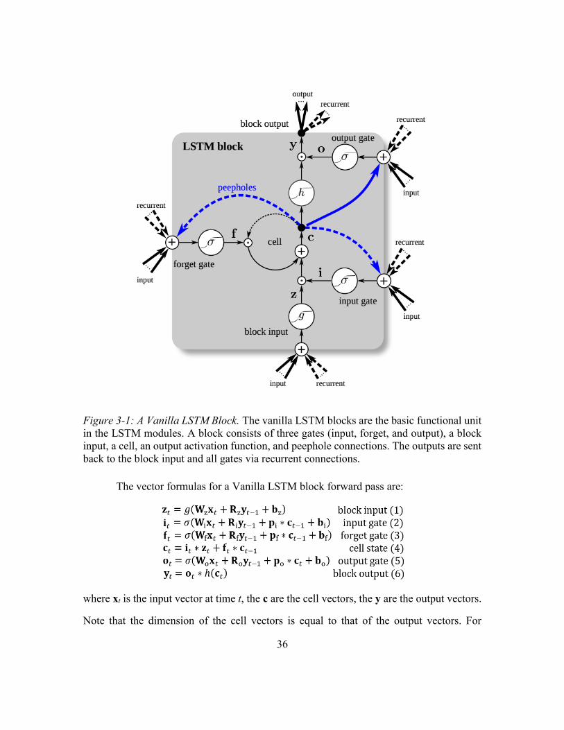
36

Figure 3-1: A Vanilla LSTM Block. The vanilla LSTM blocks are the basic functional unit

in the LSTM modules. A block consists of three gates (input, forget, and output), a block

input, a cell, an output activation function, and peephole connections. The outputs are sent

back to the block input and all gates via recurrent connections.

The vector formulas for a Vanilla LSTM block forward pass are: a ,

where xt is the input vector at time t, the c are the cell vectors, the y are the output vectors.

Note that the dimension of the cell vectors is equal to that of the output vectors. For

37

convenience of discussion, it is referred to as the cell size. The W are weight matrices for

the inputs, the R are recurrent weight matrices for the outputs, the p are peephole weight

vectors, and the b are bias vectors. The asterisks denote point-wise multiplication of two

vectors, and 𝜎, g, and h are point-wise activation functions. In this application, all LSTM

blocks use hyperbolic tangent as both input and output activation function

In recent years, LSTM neural networks have emerged as the state-of-the-art models

for a number of challenging AI problems where extraction and analysis of sequential

patterns are essential, including handwriting recognition [Doetsch et al., 2014; Graves et

al., 2008], language modeling [Zaremba et al., 2014] and translation [Luong et al., 2014],

acoustic modeling of speech [Sak et al., 2014], speech synthesis [Fan et al., 2014], and

analysis of audio [Marchi et al., 2014], etc. Hence, applying LSTM neural networks for

opponent modeling in poker is a promising new direction.

Greff et al. [2015] presented a large-scale analysis of eight LSTM variants on three

representative tasks: speech recognition, handwriting recognition, and polyphonic music

modeling. Experimental results showed that none of the variants can improve upon the

standard LSTM architecture significantly, and that the forget gate and the output activation

function to be the most critical components.

This work provides helpful insights for the design and optimization of the

architecture of opponent models based on LSTM neural networks.

3.3.2. Neuroevolution

A potential difficulty in building LSTM-based opponent models in HUNL is the

lack of training data for supervised learning. In particular, the correct outputs of certain

predictions cannot be easily obtained (e.g. what is the probability of a certain opponent

folding to a pot-size bet given current game state and the history of previous game against

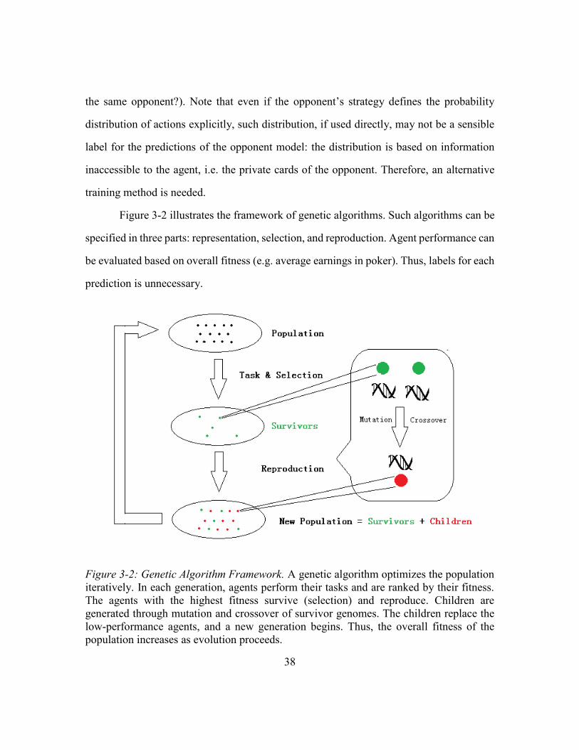
38

the same opponent?). Note that even if the opponent’s strategy defines the probability

distribution of actions explicitly, such distribution, if used directly, may not be a sensible

label for the predictions of the opponent model: the distribution is based on information

inaccessible to the agent, i.e. the private cards of the opponent. Therefore, an alternative

training method is needed.

Figure 3-2 illustrates the framework of genetic algorithms. Such algorithms can be

specified in three parts: representation, selection, and reproduction. Agent performance can

be evaluated based on overall fitness (e.g. average earnings in poker). Thus, labels for each

prediction is unnecessary.

Figure 3-2: Genetic Algorithm Framework. A genetic algorithm optimizes the population

iteratively. In each generation, agents perform their tasks and are ranked by their fitness.

The agents with the highest fitness survive (selection) and reproduce. Children are

generated through mutation and crossover of survivor genomes. The children replace the

low-performance agents, and a new generation begins. Thus, the overall fitness of the

population increases as evolution proceeds.

39

Neuroevolution (NE), the artificial evolution of neural networks using genetic

algorithms, has showed great promise in many complex reinforcement learning tasks since

its inception [Gomez and Miikkulainen, 1999; Gruau et al., 1996; Moriarty and

Miikkulainen, 1997; Potter et al., 1995; Whitley et al., 1993].

In particular, Stanley and Miikkulainen [2002] proposed Neuroevolution with

Augmented Topology (NEAT) to evolve neural network topologies along with weights.

The algorithm was extended for evolving neural networks in real time [Stanley et al. 2005].

In addition, NE algorithms were proposed to evolve deep unsupervised convolutional

network [Koutnik et al. 2014] and multi-modal neural networks [Li and Miikkulainen,

2014; Schrum and Miikkulainen, 2014].

While NEAT was initially designed to evolve feed-forward neural networks and

simple recurrent neural networks, its principles for crossover of different topologies,

protecting structural innovation using speciation, and growing incrementally from minimal

structure can be adjusted for optimizing the architecture of LSTM neural network. Bayer

et al. [2009] proposed to optimize LSTM memory cell structure through multi-objective

evolutionary algorithm. Rawal and Miikkulainen [2016] extended NEAT for evolving deep

LSTM neural networks by introducing information stored in the LSTM networks as a

secondary optimization objective.

NE searches for behaviors with highest fitness instead of a specific function. In the

context of HUNL, fitness can be evaluated by the agents’ average winning in matches

against the opponents. Thus, it can be used to evolve LSTM-based opponent models

without labeled training data.

40

3.3.3. Conclusions

Based on the above related work, the proposed dissertation aims at (1) developing

an evolutionary method for discovering opponent model based on LSTM neural networks

and (2) building high-performance adaptive poker agents using such models. Poker agents

built in this method should achieve comparable performance against state-of-the-art

equilibrium based agents. In addition, they should be able to adapt to their opponents

dynamically, even to those with stronger strategies than they have seen in training, and

exploit weak strategies effectively.

Compared to existing method, the proposed approach has several advantages. First,

this approach aims at maximizing utility rather than minimizing exploitation, potentially

producing agents with higher performance practically. Second, agents built in this method

are not bound by Nash-equilibrium strategies and can adapt their moves to exploit

opponent’s weaknesses more effectively. Third, the proposed approach does not rely on

the existence or any property of Nash equilibria in the problem domain and is therefore

applicable to a wider range of problems involving imperfect information.

Thus, the approach provides a promising new direction for research in computer

poker and imperfect information games.

41

Chapter 4: Evolving LSTM-based Opponent Models

ASHE 1.0 is the first step in devising an evolutionary approach to building

recurrent-neural-network-based computer poker agents. It serves three purposes: (1) to

validate the general methodology, (2) to devise an effective algorithmic framework that

can be used to evolve such agents, and (3) to discover key factors that influence agent

performance for further optimization.

This chapter contains four subsections. Section 4.1 details the architecture of the

system. Section 4.2 introduces the genetic algorithm to evolve the agents. Section 4.3

presents and analyzes experimental results. Section 4.4 summarizes key findings and

conclusions.

4.1. ASHE 1.0 ARCHITECTURE

Figure 4-1 illustrates the overall architecture of ASHE 1.0. The opponent module

extracts and encodes patterns in opponent strategy based on the entire game history against

the opponent, i.e. every action in every hand against the current opponent. In contrast, the

game module does not look into previous games. Instead, it focuses on the hand in play

and encodes the game states, e.g. action sequence, pot odds, expected hand strength of the

agent, etc., of that hand only. Both the opponent and the game module contain a single

layer of vanilla LSTM blocks.

The patterns and game states encoded by the LSTM modules are sent to the decision

network, whose output is a score indicating the relative strength of the agent’s hand

compared to the perceived range of the opponent’s possible holdings. Finally, the decision

algorithm selects the next move for the agent using the score and a set of rules that are

specified by human experts.

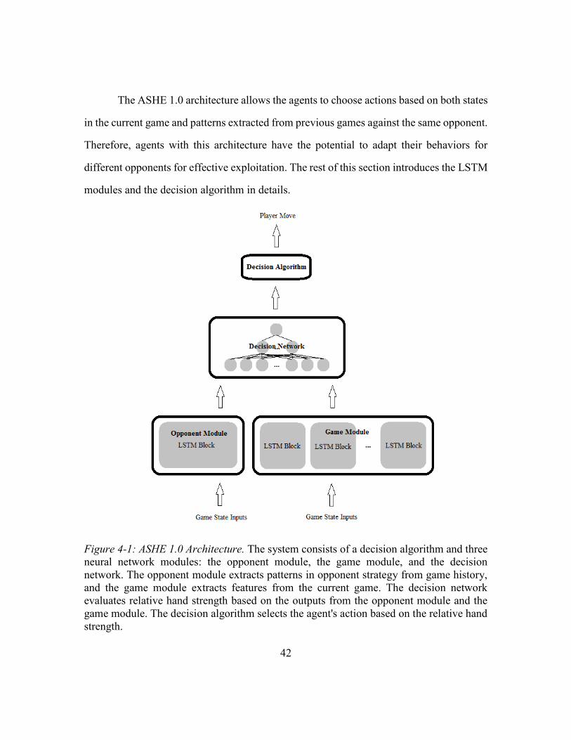
42

The ASHE 1.0 architecture allows the agents to choose actions based on both states

in the current game and patterns extracted from previous games against the same opponent.

Therefore, agents with this architecture have the potential to adapt their behaviors for

different opponents for effective exploitation. The rest of this section introduces the LSTM

modules and the decision algorithm in details.

Figure 4-1: ASHE 1.0 Architecture. The system consists of a decision algorithm and three

neural network modules: the opponent module, the game module, and the decision

network. The opponent module extracts patterns in opponent strategy from game history,

and the game module extracts features from the current game. The decision network

evaluates relative hand strength based on the outputs from the opponent module and the

game module. The decision algorithm selects the agent's action based on the relative hand

strength.

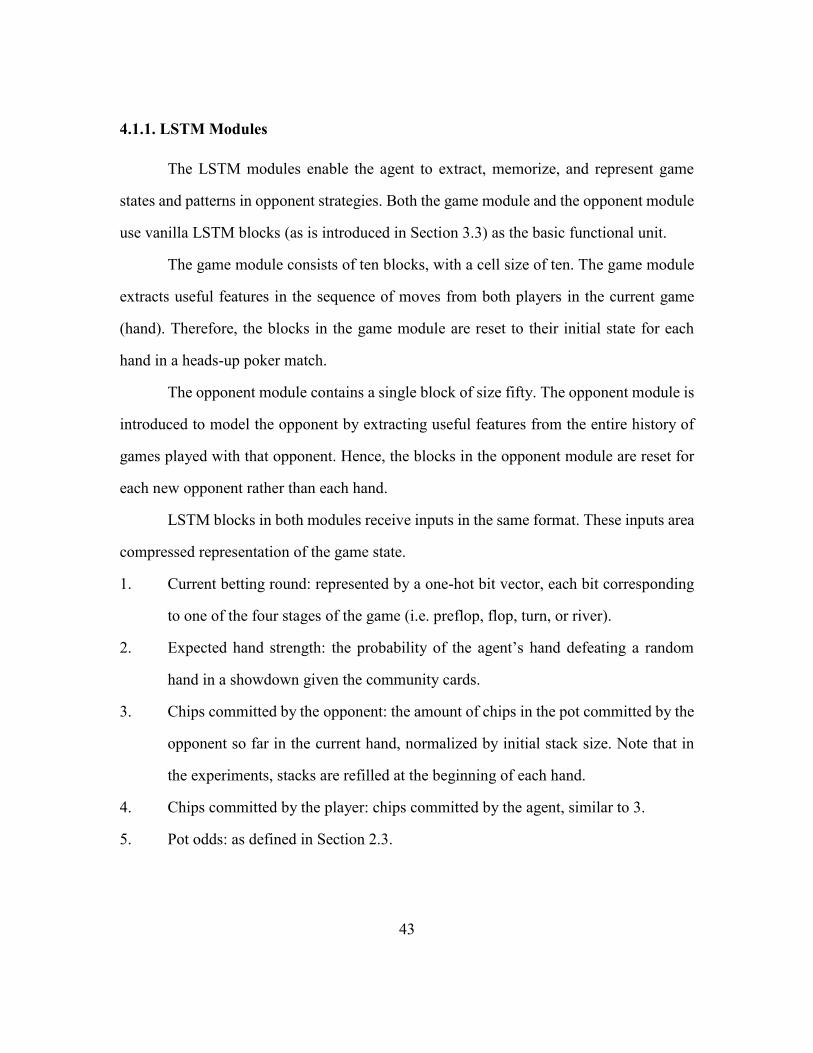
43

4.1.1. LSTM Modules

The LSTM modules enable the agent to extract, memorize, and represent game

states and patterns in opponent strategies. Both the game module and the opponent module

use vanilla LSTM blocks (as is introduced in Section 3.3) as the basic functional unit.

The game module consists of ten blocks, with a cell size of ten. The game module

extracts useful features in the sequence of moves from both players in the current game

(hand). Therefore, the blocks in the game module are reset to their initial state for each

hand in a heads-up poker match.

The opponent module contains a single block of size fifty. The opponent module is

introduced to model the opponent by extracting useful features from the entire history of

games played with that opponent. Hence, the blocks in the opponent module are reset for

each new opponent rather than each hand.

LSTM blocks in both modules receive inputs in the same format. These inputs area

compressed representation of the game state.

1. Current betting round: represented by a one-hot bit vector, each bit corresponding

to one of the four stages of the game (i.e. preflop, flop, turn, or river).

2. Expected hand strength: the probability of the agent’s hand defeating a random

hand in a showdown given the community cards.

3. Chips committed by the opponent: the amount of chips in the pot committed by the

opponent so far in the current hand, normalized by initial stack size. Note that in

the experiments, stacks are refilled at the beginning of each hand.

4. Chips committed by the player: chips committed by the agent, similar to 3.

5. Pot odds: as defined in Section 2.3.

44

The LSTM blocks are organized into layers and serves as the core component in

both LSTM modules, allowing the agent to decide its actions based on game states of the

current hand and patterns extracted from previous games against the same opponent.

4.1.2. Decision Network and Decision Algorithm

The decision network and algorithm decide the next action of the agent using the

outputs from the LSTM modules. The outputs of the LSTM blocks in the game module

and the opponent module are concatenated as an input vector to the decision network. The

decision network is a fully-connected feed-forward neural network with one hidden layer.

In ASHE 1.0, the decision network has a single real valued output o, where −1 < 𝑜 < 1.

The output can be considered as an aggression score indicating how aggressive ASHE’s

next action should be, with -1 and 1 indicating the least and most aggressive, respectively.

Figure 4-2: ASHE 1.0 Decision Algorithm. The decision algorithm selects the next action

for the agent based on the output o from the decision network. The variable ss is the stack

size at the start of the game, x is the amount to call, BB is the big blind, rmin is the minimum

raise, and y can be considered as the amount of extra chips the player is willing to commit.

Figure 4-3 presents the decision algorithm in ASHE 1.0. The algorithm uses a

straight-forward rule-based approach to decide the next move. If a call is decided but

current stack is too short to call, the agent goes all-in instead. In the case of a raise, k ∙ BB

is the amount of extra chips committed to the pot, and k ∙ BB - x is technically the raise

amount. The actual number of chips committed in a raise is converted to integer times of

45

the big blind. Similar to the case of a call, if current stack is too short for a decided raise,

the player goes all-in. The decision algorithm in ASHE 1.0 takes advantage of opponent

modeling through the aggression score, i.e. o, which is computed using features extracted

by the LSTM modules from both the current and the previous games.

The algorithm has two limitations. First, it does not take possible future actions into

consideration. Second, its level of aggression strongly correlates with the relative hand

strength. Thus, it is unable to trap the opponent with tactics such as check-raising and slow-

playing. However, even with the above limitations, this simplified decision algorithm

combined with the LSTM modules and the decision network is sufficient for the agents to

demonstrate adaptive behaviors and exploit different opponents, achieving much stronger

performance against weak opponents than top-ranking equilibrium-based poker agents.

4.2. METHOD OF EVOLVING ADAPTIVE AGENTS

This section introduces the genetic algorithm to evolve adaptive RNN-based agents

for imperfect information games. Subsection 4.2.1 describes the motivation of using

genetic algorithms. Subsection 4.2.2 outlines the algorithmic framework and discusses key

technical points.

4.2.1. Motivation

While gradient-based approaches for training LSTM neural networks are most

commonly used, they require sufficient training samples with correct labels. In poker, the

correct label translates into the optimal action for a given game state (i.e. private cards,

community cards, action sequence, etc.) and a specific opponent. However, such training

data generally do not exist and are infeasible to obtain, because the optimal actions are

usually unknown or undefined. Even the best professional players often disagree on what

46

the correct move should be when analyzing poker games, especially when the opponent's

strategy is taken into consideration.

In contrast, evolutionary methods do not require any labeled training data. The

agents can be trained as long as an appropriate fitness function is provided to reflect their

overall performance. In other words, the agents are evaluated and optimized based on their

overall performance, e.g. in poker, their average earnings, and the value of each action is

unnecessary.

A major technical insight in this research is that it is possible to evolve RNN-based

agents for imperfect information games through genetic algorithms. This approach allows

the method to be applied to problems with little or no labeled training data.

4.2.2. Evolutionary Method

Since the Vanilla LSTM blocks in the opponent module and the game module have

a fixed structure, and the decision network has a fixed structure as well, the genetic

representation of an agent can be constructed by serializing and concatenating weight

matrices, weight vectors, bias vectors, etc., of all components.

In order to encourage adaptation, the selection process must allow players to play

against opponents with a variety of exploitable strategies. These strategies should require

different and preferably opposite counter-strategies for maximum exploitation. Fitness

functions should evaluate a player based on its performance against all opponents. In

particular, bias must be taken into consideration to prevent experts specialized in exploiting

certain types of opponents from constantly dominating the population. For example,

exploiting a player who goes all-in every hand can generate far more earnings than

exploiting a player who folds to any bets. If the fitness function evaluates agents'

performance by simply adding up their earnings against each opponent, the population may

47

focus on a few opponents that generate high earnings while ignoring the others, resulting

in specialized rather than adaptive behaviors.

Stochasticity in imperfect information games presents an additional challenge to

the selection process. For example, the length of game sessions for evaluation must be

chosen carefully. If the sessions are too short, high-quality agents are likely to lose due to

bad luck. On the other hand, long game sessions may render selection painfully slow.

Similarly, a small survival rate may eliminate many unlucky good players, while a large

survival rate may preserve poor genotypes and reduce performance of future generations.

Furthermore, genomes of adaptive LSTM players tend to be sizable, making it relatively

difficult to discover and propagate advantageous genotypes via mutation and crossover.

To alleviate these problems, the Tiered Survival and Elite Reproduction (TSER)

method was developed in this dissertation. Survivors of a generation are divided into two

tiers based on their fitness. Only members of the top tier, i.e. the elites, are allowed to

reproduce. They are immune to mutation as long as they remain in the top tier. Members

of the second tier are not allowed to reproduce, neither are they immune to mutation.

However, survival provides them the opportunity to preserve advantageous genotypes and

improve performance through mutation.

In each generation, all players are evaluated in the same way regardless of their

status. Thus, second-tier survivors from previous generations and newborn players in the

latest generation can compete for positions in the top tier. After survivors are selected and

classified, crossover takes place between randomly selected elites to construct genomes for

the next generation. After crossover, children and second-tier survivor genomes are

mutated.

TSER has three advantages. First, advantageous genotypes are not lost even if they

perform poorly occasionally, because they can survive in the second tier. Second, the

48

survival rate dilemma no longer exists. A high survival rate coupled with a small top tier

can keep poor genotypes from being propagated while reducing accidental losses of

desirable genotypes. Third, because advantageous genotypes among elites are immune to

mutation, they are preserved for multiple generations, thereby providing them more time

to be propagated among entire population.

To balance exploration of genome space and preservation of advantageous

genotype, descending mutation rate and strength is introduced. High mutation rate and

strength in early stage of evolution allows more effective exploration of the genome space.

As evolution proceeds, more advantageous genotypes are discovered, making less

aggressive mutation preferable.

The evolutionary method in this section provides an algorithmic framework for

evolving adaptive LSTM-based agents for large-scale imperfect information games.

4.3. EXPERIMENTAL RESULTS

This section presents experimental results and evaluates the effectiveness of the

method outlined in previous sections. Subsection 4.3.1 provides details on experimental

setup, including opponents, fitness evaluation, and parameter settings. Subsection 4.3.2

presents and analyzes ASHE 1.0’s performance against opponents with high exploitability.

Subsection 4.3.3 discusses the performance against Slumbot 2016, a Nash-equilibrium-

based player with low exploitability.

4.3.1. Experimental Setup

As stated in the previous section, selection and fitness evaluation play a key role in

evolution. To encourage adaptation, players need to be evaluated by their performance

against multiple opponents with different strategies. Fitness function needs to reward good

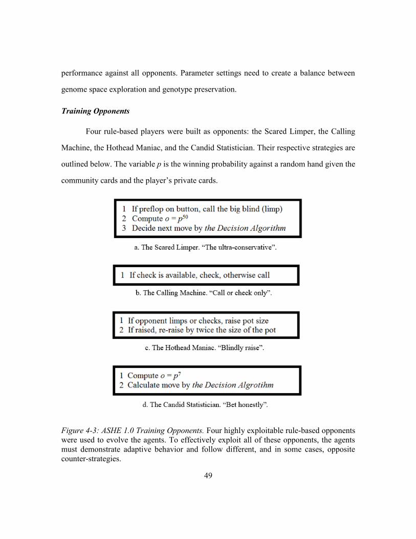
49

performance against all opponents. Parameter settings need to create a balance between

genome space exploration and genotype preservation.

Training Opponents

Four rule-based players were built as opponents: the Scared Limper, the Calling

Machine, the Hothead Maniac, and the Candid Statistician. Their respective strategies are

outlined below. The variable p is the winning probability against a random hand given the

community cards and the player’s private cards.

Figure 4-3: ASHE 1.0 Training Opponents. Four highly exploitable rule-based opponents

were used to evolve the agents. To effectively exploit all of these opponents, the agents

must demonstrate adaptive behavior and follow different, and in some cases, opposite

counter-strategies.

50

The Scared Limper always calls the big blind when being the small blind and folds

to almost any raise at any stage of the game unless holding top hands (i.e. winning

probability close to one). Counter-strategy against the Scared Limper is simple: raise any

hand regardless of hand strength; if called or re-raised, fold unless holding the best hand.

The Calling Machine stays in the game for a showdown regardless of hand strength.

To effectively exploit its weakness, players must refrain from bluffing and raise

aggressively when holding strong hands.

The Hothead Maniac is addicted to bluffing. Similar to the Calling Machine, it is

immune to bluffs. The counter-strategy must take pot control into consideration, i.e. it must

avoid inflating the pot when holding speculative hand (e.g. a flush draw) and/or moderately

strong hands (e.g. a middle pair). Folding becomes necessary when holding weak hands.

The Candid Statistician’s moves always reflect its hand strength. Bluffing can be

effective when the Candid Statistician holds a weak hand. In addition, the moves from the

Candid Statistician can be viewed as an accurate measure of its hand strength, making it

much easier for its opponent to take correct actions.

Evaluation and Selection

In each generation, every LSTM player plays against all four opponents. Two game

sessions are played with each opponent. Both sessions contain 500 hands. Card decks in

the first session are duplicated and played again in the second session. The players switch

seats between the two sessions, and the memory of the LSTM player is cleared before

entering the second session. At the beginning of each game, the chip stacks of the two

participants are reset to $20,000. The big blind of the game is $100, and no ante is required.

Cumulative earnings (i.e. the total earnings of 1000 hands in two sessions) against every

opponent is recorded for all LSTM players.

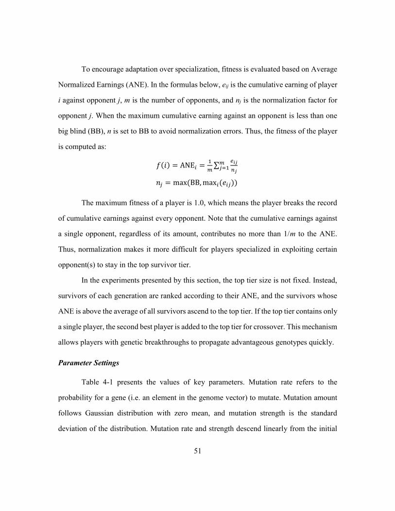
51

To encourage adaptation over specialization, fitness is evaluated based on Average

Normalized Earnings (ANE). In the formulas below, eij is the cumulative earning of player

i against opponent j, m is the number of opponents, and nj is the normalization factor for

opponent j. When the maximum cumulative earning against an opponent is less than one

big blind (BB), n is set to BB to avoid normalization errors. Thus, the fitness of the player

is computed as:

𝑓(𝑖) = ANE𝑖 =1

𝑚∑

𝑒𝑖𝑗

𝑛𝑗

𝑚𝑗=1 ,

𝑛𝑗 = max (BB, max𝑖(𝑒𝑖𝑗)),

The maximum fitness of a player is 1.0, which means the player breaks the record

of cumulative earnings against every opponent. Note that the cumulative earnings against

a single opponent, regardless of its amount, contributes no more than 1/m to the ANE.

Thus, normalization makes it more difficult for players specialized in exploiting certain

opponent(s) to stay in the top survivor tier.

In the experiments presented by this section, the top tier size is not fixed. Instead,

survivors of each generation are ranked according to their ANE, and the survivors whose

ANE is above the average of all survivors ascend to the top tier. If the top tier contains only

a single player, the second best player is added to the top tier for crossover. This mechanism

allows players with genetic breakthroughs to propagate advantageous genotypes quickly.

Parameter Settings

Table 4-1 presents the values of key parameters. Mutation rate refers to the

probability for a gene (i.e. an element in the genome vector) to mutate. Mutation amount

follows Gaussian distribution with zero mean, and mutation strength is the standard

deviation of the distribution. Mutation rate and strength descend linearly from the initial

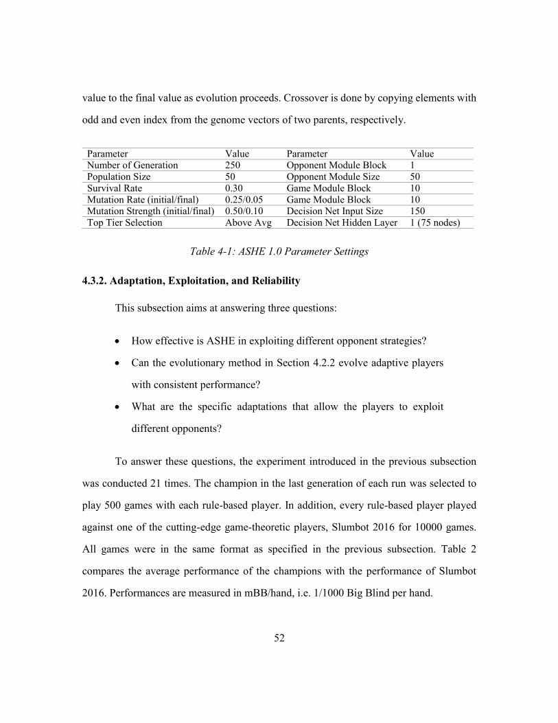
52

value to the final value as evolution proceeds. Crossover is done by copying elements with

odd and even index from the genome vectors of two parents, respectively.

Parameter Value Parameter Value Number of Generation 250 Opponent Module Block 1

Population Size 50 Opponent Module Size 50

Survival Rate 0.30 Game Module Block 10

Mutation Rate (initial/final) 0.25/0.05 Game Module Block 10 Mutation Strength (initial/final) 0.50/0.10 Decision Net Input Size 150

Top Tier Selection Above Avg Decision Net Hidden Layer 1 (75 nodes)

Table 4-1: ASHE 1.0 Parameter Settings

4.3.2. Adaptation, Exploitation, and Reliability

This subsection aims at answering three questions:

How effective is ASHE in exploiting different opponent strategies?

Can the evolutionary method in Section 4.2.2 evolve adaptive players

with consistent performance?

What are the specific adaptations that allow the players to exploit

different opponents?

To answer these questions, the experiment introduced in the previous subsection

was conducted 21 times. The champion in the last generation of each run was selected to

play 500 games with each rule-based player. In addition, every rule-based player played

against one of the cutting-edge game-theoretic players, Slumbot 2016 for 10000 games.

All games were in the same format as specified in the previous subsection. Table 2

compares the average performance of the champions with the performance of Slumbot

2016. Performances are measured in mBB/hand, i.e. 1/1000 Big Blind per hand.

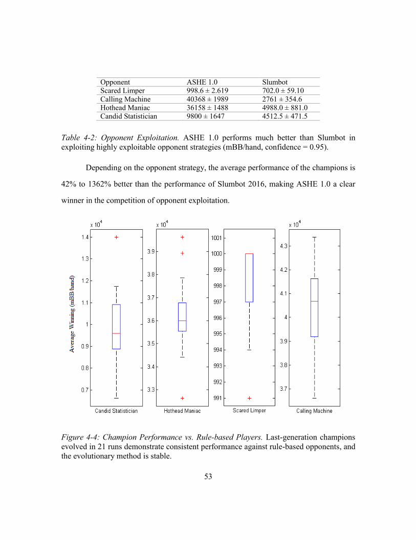
53

Opponent ASHE 1.0 Slumbot Scared Limper 998.6 ± 2.619 702.0 ± 59.10

Calling Machine 40368 ± 1989 2761 ± 354.6 Hothead Maniac 36158 ± 1488 4988.0 ± 881.0 Candid Statistician 9800 ± 1647 4512.5 ± 471.5

Table 4-2: Opponent Exploitation. ASHE 1.0 performs much better than Slumbot in

exploiting highly exploitable opponent strategies (mBB/hand, confidence = 0.95).

Depending on the opponent strategy, the average performance of the champions is

42% to 1362% better than the performance of Slumbot 2016, making ASHE 1.0 a clear

winner in the competition of opponent exploitation.

Figure 4-4: Champion Performance vs. Rule-based Players. Last-generation champions

evolved in 21 runs demonstrate consistent performance against rule-based opponents, and

the evolutionary method is stable.

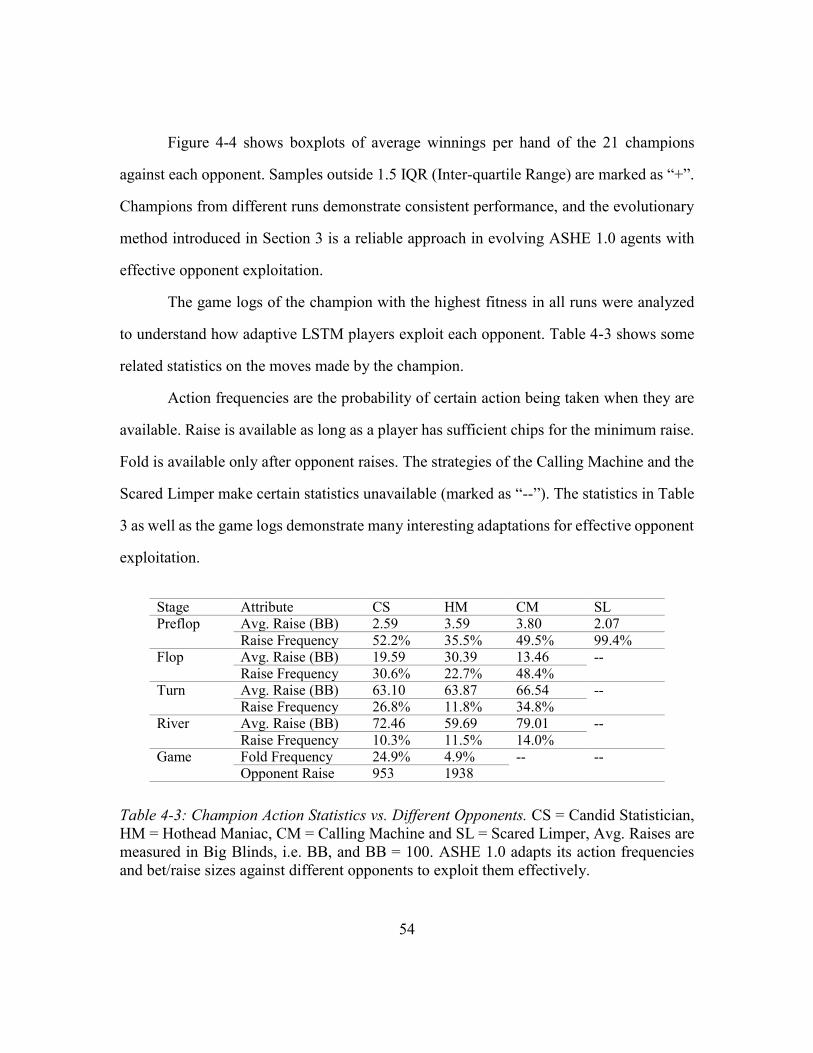
54

Figure 4-4 shows boxplots of average winnings per hand of the 21 champions

against each opponent. Samples outside 1.5 IQR (Inter-quartile Range) are marked as “+”.

Champions from different runs demonstrate consistent performance, and the evolutionary

method introduced in Section 3 is a reliable approach in evolving ASHE 1.0 agents with

effective opponent exploitation.

The game logs of the champion with the highest fitness in all runs were analyzed

to understand how adaptive LSTM players exploit each opponent. Table 4-3 shows some

related statistics on the moves made by the champion.

Action frequencies are the probability of certain action being taken when they are

available. Raise is available as long as a player has sufficient chips for the minimum raise.

Fold is available only after opponent raises. The strategies of the Calling Machine and the

Scared Limper make certain statistics unavailable (marked as “--”). The statistics in Table

3 as well as the game logs demonstrate many interesting adaptations for effective opponent

exploitation.

Stage Attribute CS HM CM SL Preflop Avg. Raise (BB) 2.59 3.59 3.80 2.07

Raise Frequency 52.2% 35.5% 49.5% 99.4% Flop Avg. Raise (BB) 19.59 30.39 13.46 --

Raise Frequency 30.6% 22.7% 48.4% Turn Avg. Raise (BB) 63.10 63.87 66.54 --

Raise Frequency 26.8% 11.8% 34.8% River Avg. Raise (BB) 72.46 59.69 79.01 --

Raise Frequency 10.3% 11.5% 14.0% Game Fold Frequency 24.9% 4.9% -- --

Opponent Raise 953 1938

Table 4-3: Champion Action Statistics vs. Different Opponents. CS = Candid Statistician,

HM = Hothead Maniac, CM = Calling Machine and SL = Scared Limper, Avg. Raises are

measured in Big Blinds, i.e. BB, and BB = 100. ASHE 1.0 adapts its action frequencies

and bet/raise sizes against different opponents to exploit them effectively.

55

First, the fold frequency of the champion when playing against the Candid

Statistician is four times higher than the fold frequency against the Hothead Maniac. The

champion adapts to the fact that the Candid Statistician’s raises indicate strong hands, while

the Hothead Maniac is inclined to bluff. Second, to exploit the strategy of the Scared

Limper, the champion increases preflop raise frequency to nearly 100%, forcing the

extremely-conservative opponent to fold almost every hand. Third, when playing against

the Hothead Maniac, the champion’s raise frequency is much lower in all stages of the

game. However, the average raises from the champion at the turn and the river are both

close to 60 BBs. Note that a raise over 40 BBs ($4,000) generally leads to an all-in due to

the Hothead Maniac’s strategy and the size of the stack ($20,000). Thus, the champion

exploits Hothead Maniac’s strategy by folding weak hands, calling with fair hands, and

inducing all-in with strong hands. Fourth, the champion’s strategy against the Calling

Machine features much higher raise frequency compared to its strategy against the Hothead

Maniac. Game logs indicate that the champion is not bluffing. Rather, it simply recognizes

the fact that the Calling Machine’s moves are independent from the strength of its hands.

Therefore, if the champion’s hand is better than the average, it raises. In addition, the

amount of a raise is strongly correlated with hand strength, which is different from the

strategy against the Candid Statistician where the champion plays strong hands less

aggressively and bluffs when the opponent appears passive.

Such adaptations enable ASHE 1.0 agents to make more profitable moves against

different players, thus exploiting the weakness of opponent strategy effectively.

4.3.3. Slumbot Challenge

ASHE 1.0 agents are evolved through playing against rule-based players with only

simple, weak strategies. Generally, genetic algorithms tend to achieve no fitness beyond

56

the scope of evolution. Nevertheless, adaptive players have the potential to compete against

previously unseen opponents through adaptation. How well can they generalize against

new opponents with much stronger strategies?

To answer this question, 500 games were played between the champions from each

run (as introduced in the previous subsection) and Slumbot 2016. The adaptive players lost

to Slumbot 2016 by an average of 426 mBB/hand.

Game logs show that ASHE 1.0 adopts an aggressive strategy that is essentially a

biased combination of the strategies against the rule-based players, and is able to bluff

Slumbot 2016 effectively when holding relatively weak hands. However, Slumbot 2016

performs much better when holding strong hands. In particular, Slumbot 2016 uses value

bets (i.e. small to mid-sized bets aimed at inducing a call or re-raise) effectively. In contrast,

ASHE 1.0 tends to raise rather aggressively with a strong hand, which usually reveals true

hand strength and leads to a fold in response.

This problem may be caused by the fact that ASHE 1.0 agents have rarely seen

value bets from the rule-based opponents; neither is value bet necessary for exploiting

them. Two out of the four rule-based players almost never fold to any raise. Furthermore,

the Candid Statistician can be quite reckless in calling or raising when the pot is small.

To alleviate this problem, two adjustments were made to the decision algorithm:

(1) raise amount was restricted to be integer times of a half of the pot size, up to twice the

pot size and all-in, and (2) if the desired raise amount was smaller than a fourth of the pot

size, the player was made to call or check instead of raise. These rule-based adjustments

limit raise amount to five options, making each option representing a much wider range of

hands, which helps conceal true hand strength. After the adjustments, the agents’

performance improved considerably, losing 115 mBB/hand, or approximately 1/10 of a big

blind per hand against Slumbot 2016.

57

These results suggest that ASHE 1.0 agents can adapt to opponents that are not seen

in training by combining strategies against the training opponents. However, when the

opponent is significantly stronger than the training opponents, such as Slumbot 2016, it

still loses in heads-up matches against it.

4.4. DISCUSSION AND CONCLUSION

ASHE 1.0 is the first attempt in evolving an adaptive recurrent-neural-network-

based computer agent for HUNL, which is considered one of the most challenging

imperfect information games. The system lays a solid foundation for this line of research

and provides valuable insights into the methodology.

First, the experimental results showed that LSTM neural networks can be leveraged

to represent game states and model opponent strategies. The ASHE 1.0 architecture enables

the agents to adapt their behaviors, thereby exploiting different opponents. In particular,

when facing opponents with highly exploitable strategies, the adaptive agents are

significantly more effective than top-ranking equilibrium-based agents. Second, ASHE 1.0

presents an algorithmic framework for evolving adaptive RNN-based agents for HUNL

and other imperfect information games. Such evolutionary methods do not require labeled

training data and are therefore applicable to a wider range of problems. The TSER method

preserves advantageous genotypes while creating high-quality offspring, and is particularly

effective in evolving computer agents for games of chance. Third, the experimental results

show that the evolutionary method is reliable, i.e. the agents generated from different runs

demonstrate consistent performance. Fourth, ASHE 1.0 can adapt to opponents that are not

seen during training by combining strategies learned through evolution. However, if the

opponents are much stronger than the training opponents, it still loses in a heads-up match.

58

Thus, the empirical results and analysis of ASHE 1.0 validate the methodology.

They also point out potential directions for further improvement. From an architectural

perspective, ideally, the LSTM module, and in particular, the opponent module should

contain enough blocks to extract and encode all useful features. This design is especially

important when playing against more sophisticated opponents, as exploitable patterns in

their strategies tend to be conditional and well-hidden. On the other hand, evolving bigger

networks is generally less efficient. Hence, the first challenge is to develop an architecture

that uses (relatively) small LSTM modules to extract and encode sufficient features in

opponent strategies.

In addition, ASHE 1.0 models the opponents implicitly. It does not predict the

opponent’s actions or estimate the opponent’s (expected) hand strength directly. In fact, all

information on the game states of the hand in play and the opponent’s strategy is

represented by the aggression score, i.e. the output of the decision network. Implicit

opponent modeling makes it difficult to estimate the expected value for possible actions.

Hence, ASHE 1.0 adopts an intuitive rule-based approach to select the next action based

on the aggression score. Such intuitive methods may be effective against opponents with

relatively simple strategies. However, their performance against strong opponents, e.g.

Slumbot 2016, is unsatisfactory.

Therefore, the second direction is explicit opponent modeling, i.e. to predict hand

strength, opponent actions, etc. The prediction can be used to estimate the expected values

for possible actions, thus allowing the agents to make more accurate decisions. The next

chapter introduces ASHE 2.0, an upgrade of the system that addresses both of these

problems.

59

Chapter 5: Pattern Recognition Tree and Explicit Modeling

This chapter introduces ASHE 2.0, which establishes an effective and extensible

architectural framework for building LSTM-based adaptive agents for HUNL and other


Compared to the previous version, ASHE 2.0 makes two improvements. First, it

introduces the Pattern Recognition Tree (PRT), which enhances the ability of modeling

complex opponent strategies while keeping the LSTM modules small enough for efficient

evolution. Second, it models the opponents explicitly, thus allowing the agents to make

decisions by estimating the expected utility of each available action.

Experimental results show that ASHE 2.0 models and exploits both weak and

strong opponents effectively. In particular, it achieves significantly better performance in

matches against top-ranking equilibrium opponents than the previous version and tied

statistically with Slumbot 2017, an upgraded and much stronger version of Slumbot 2016,

which was used in the ASHE 1.0 experiments.

This chapter consists of four sections. Section 5.1 introduces the architecture of

ASHE 2.0. Section 5.2 introduces the genetic algorithm to evolve the agents. Section 5.3

presents and analyzes the experimental results. Section 5.4 summarizes the findings and

discusses directions for further improvements.


The ASHE 2.0 architecture is an RNN-based architectural framework that enables

the agents to capture more subtle patterns in opponent strategies through explicit opponent

modeling. The architecture allows efficient training by the evolutionary methods specified

in Chapter 4, and is effective against opponents that are much stronger than opponents seen

during evolution.

60

Subsection 5.1.1 presents the overall architecture and introduces the motivation of

the design. Subsection 5.1.2 and subsection 5.1.3 focuses on the components, e.g. the

opponent model and the decision algorithm, respectively.

5.1.1. Motivation and Framework

The ASHE 2.0 architecture builds on ASHE 1.0 by expanding the opponent model.

Instead of the LSTM modules only, it now contains the Pattern Recognition Tree (PRT)

and two LSTM estimators. The PRT and the LSTM estimators extract exploitable patterns,

predicts opponent moves, and estimate showdown value based on opponent hand strength.

In addition, ASHE 2.0 decides its moves based on action utilities estimation instead of the

aggression score as in ASHE 1.0. The decision algorithm evaluates the expected utility of

each available action using the outputs of the opponent model, and selects the action with

the highest utility (Figure 5-1).

Motivation: Pattern Recognition Tree

As is presented in Chapter 4, ASHE 1.0 achieved remarkable performance against

highly exploitable opponents through implicit opponent modeling and adaptation.

However, it was less effective playing against Nash-equilibrium-based opponents whose

strategy is considerably less exploitable. This result is attributable to the fact that the

exploitable patterns of strong opponents are usually conditional and difficult to discover.

For instance, Slumbot 2016 (the version in ASHE 1.0 experiments) tends to underestimate

its hand value when facing a paired board. Thus, bluffing on paired-flops is a profitable

move against this agent in the long run. As another example, when holding a two-card flush

draw on the flop, Slumbot 2016 semi-bluffs noticeably more often than most players. Since

a flush draw hits only (roughly) 1/3 of the time, this pattern can be exploited by continuing

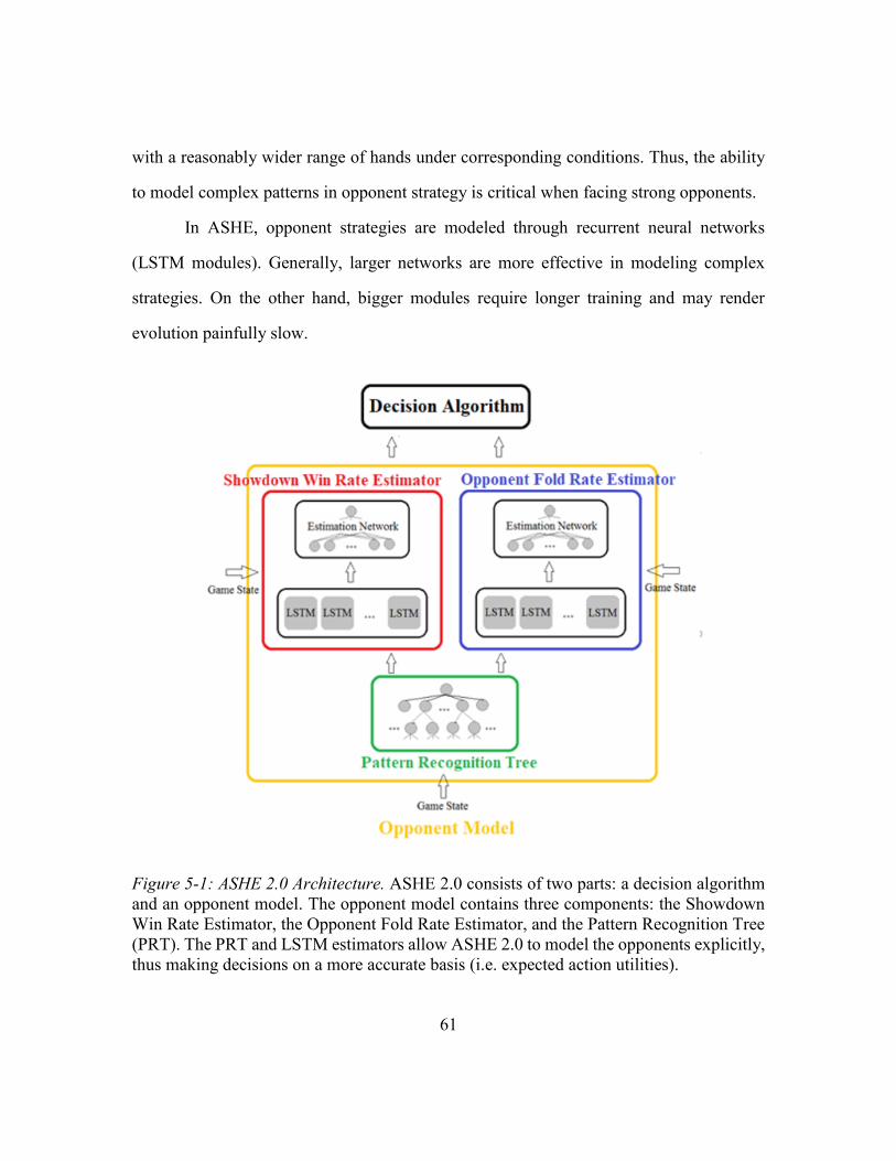
61

with a reasonably wider range of hands under corresponding conditions. Thus, the ability

to model complex patterns in opponent strategy is critical when facing strong opponents.

In ASHE, opponent strategies are modeled through recurrent neural networks

(LSTM modules). Generally, larger networks are more effective in modeling complex

strategies. On the other hand, bigger modules require longer training and may render

evolution painfully slow.

Figure 5-1: ASHE 2.0 Architecture. ASHE 2.0 consists of two parts: a decision algorithm

and an opponent model. The opponent model contains three components: the Showdown

Win Rate Estimator, the Opponent Fold Rate Estimator, and the Pattern Recognition Tree

(PRT). The PRT and LSTM estimators allow ASHE 2.0 to model the opponents explicitly,

thus making decisions on a more accurate basis (i.e. expected action utilities).

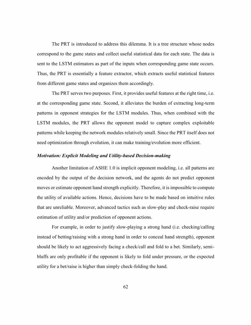
62

The PRT is introduced to address this dilemma. It is a tree structure whose nodes

correspond to the game states and collect useful statistical data for each state. The data is

sent to the LSTM estimators as part of the inputs when corresponding game state occurs.

Thus, the PRT is essentially a feature extractor, which extracts useful statistical features

from different game states and organizes them accordingly.

The PRT serves two purposes. First, it provides useful features at the right time, i.e.

at the corresponding game state. Second, it alleviates the burden of extracting long-term

patterns in opponent strategies for the LSTM modules. Thus, when combined with the

LSTM modules, the PRT allows the opponent model to capture complex exploitable

patterns while keeping the network modules relatively small. Since the PRT itself does not

need optimization through evolution, it can make training/evolution more efficient.

Motivation: Explicit Modeling and Utility-based Decision-making

Another limitation of ASHE 1.0 is implicit opponent modeling, i.e. all patterns are

encoded by the output of the decision network, and the agents do not predict opponent

moves or estimate opponent hand strength explicitly. Therefore, it is impossible to compute

the utility of available actions. Hence, decisions have to be made based on intuitive rules

that are unreliable. Moreover, advanced tactics such as slow-play and check-raise require

estimation of utility and/or prediction of opponent actions.

For example, in order to justify slow-playing a strong hand (i.e. checking/calling

instead of betting/raising with a strong hand in order to conceal hand strength), opponent

should be likely to act aggressively facing a check/call and fold to a bet. Similarly, semi-

bluffs are only profitable if the opponent is likely to fold under pressure, or the expected

utility for a bet/raise is higher than simply check-folding the hand.

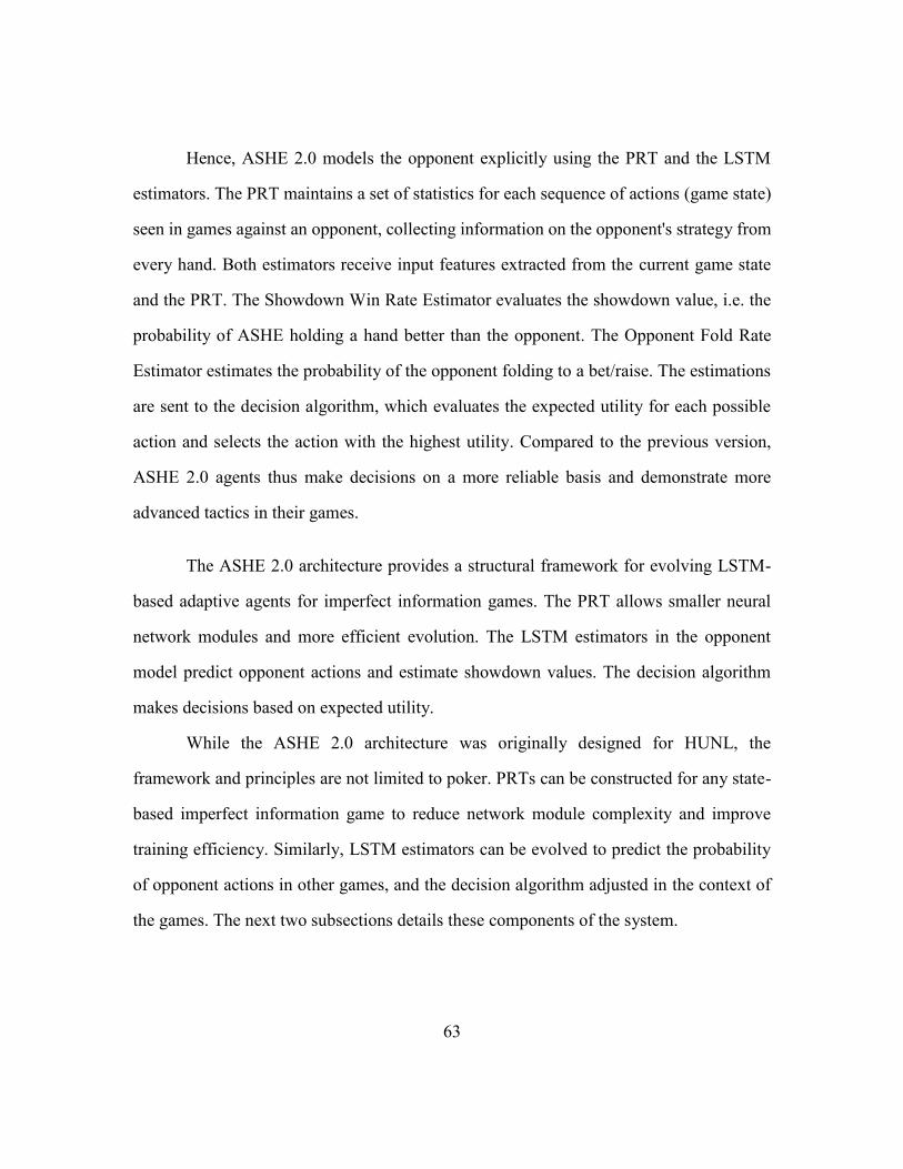
63

Hence, ASHE 2.0 models the opponent explicitly using the PRT and the LSTM

estimators. The PRT maintains a set of statistics for each sequence of actions (game state)

seen in games against an opponent, collecting information on the opponent's strategy from

every hand. Both estimators receive input features extracted from the current game state

and the PRT. The Showdown Win Rate Estimator evaluates the showdown value, i.e. the

probability of ASHE holding a hand better than the opponent. The Opponent Fold Rate

Estimator estimates the probability of the opponent folding to a bet/raise. The estimations

are sent to the decision algorithm, which evaluates the expected utility for each possible

action and selects the action with the highest utility. Compared to the previous version,

ASHE 2.0 agents thus make decisions on a more reliable basis and demonstrate more

advanced tactics in their games.

The ASHE 2.0 architecture provides a structural framework for evolving LSTM-

based adaptive agents for imperfect information games. The PRT allows smaller neural

network modules and more efficient evolution. The LSTM estimators in the opponent

model predict opponent actions and estimate showdown values. The decision algorithm

makes decisions based on expected utility.

While the ASHE 2.0 architecture was originally designed for HUNL, the

framework and principles are not limited to poker. PRTs can be constructed for any state-

based imperfect information game to reduce network module complexity and improve

training efficiency. Similarly, LSTM estimators can be evolved to predict the probability

of opponent actions in other games, and the decision algorithm adjusted in the context of

the games. The next two subsections details these components of the system.

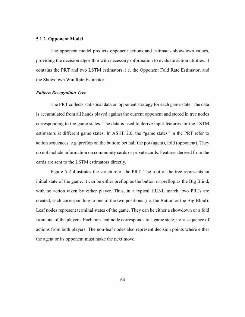
64

5.1.2. Opponent Model

The opponent model predicts opponent actions and estimates showdown values,

providing the decision algorithm with necessary information to evaluate action utilities. It

contains the PRT and two LSTM estimators, i.e. the Opponent Fold Rate Estimator, and

the Showdown Win Rate Estimator.

Pattern Recognition Tree

The PRT collects statistical data on opponent strategy for each game state. The data

is accumulated from all hands played against the current opponent and stored in tree nodes

corresponding to the game states. The data is used to derive input features for the LSTM

estimators at different game states. In ASHE 2.0, the “game states” in the PRT refer to

action sequences, e.g. preflop on the button: bet half the pot (agent), fold (opponent). They

do not include information on community cards or private cards. Features derived from the

cards are sent to the LSTM estimators directly.

Figure 5-2 illustrates the structure of the PRT. The root of the tree represents an

initial state of the game: it can be either preflop as the button or preflop as the Big Blind,

with no action taken by either player. Thus, in a typical HUNL match, two PRTs are

created, each corresponding to one of the two positions (i.e. the Button or the Big Blind).

Leaf nodes represent terminal states of the game. They can be either a showdown or a fold

from one of the players. Each non-leaf node corresponds to a game state, i.e. a sequence of

actions from both players. The non-leaf nodes also represent decision points where either

the agent or its opponent must make the next move.

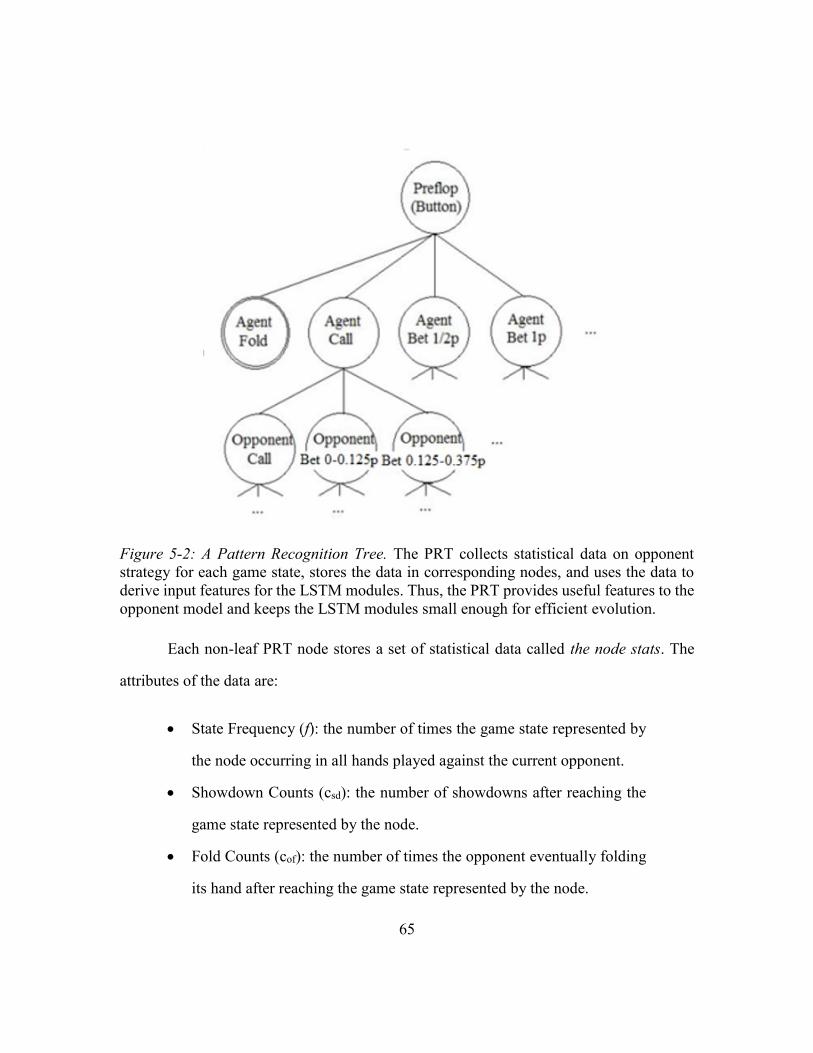
65

Figure 5-2: A Pattern Recognition Tree. The PRT collects statistical data on opponent

strategy for each game state, stores the data in corresponding nodes, and uses the data to

derive input features for the LSTM modules. Thus, the PRT provides useful features to the

opponent model and keeps the LSTM modules small enough for efficient evolution.

Each non-leaf PRT node stores a set of statistical data called the node stats. The

attributes of the data are:

State Frequency (f): the number of times the game state represented by

the node occurring in all hands played against the current opponent.

Showdown Counts (csd): the number of showdowns after reaching the

game state represented by the node.

Fold Counts (cof): the number of times the opponent eventually folding

its hand after reaching the game state represented by the node.

66

Showdown Strength ( �̅� ): the average opponent hand strength in all

showdowns after passing the game state represented by the node.

The node stats capture patterns in the opponent strategy at different game states.

For instance, if the opponent is over-cautious when facing consecutive bets at both the flop

and the turn, the cof will be high for every node along that path, suggesting an opportunity

for bluffing. At the beginning of a match, two PRTs corresponding to each position (i.e.

the button and the Big Blind) are initialized with only a root node. Nodes are inserted to

the trees when their corresponding game states occur for the first time in the match.

Suppose in the first hand of a game session, ASHE plays the button and decides to

call the Big Blind preflop, a node representing that action will be added as a child of the

root. At this point, all attributes in the node stats are set to null and cannot be used for

deriving input features to the LSTM estimators. Instead, a set of default inputs are sent to

the estimators. Suppose the opponent decides to raise by two Big Blinds, a node

representing the raise will be added to the PRT as a child of the node that represents

ASHE’s call. This process continues until the current hand is finished.

After each hand, node stats in non-leaf nodes along the path (from the root to the

leaf) will be updated based on the result of the game. State frequencies of the nodes will

be increased by one. If the opponent folds in the end, fold counts of the nodes will be

increased by one. If a showdown occurs, showdown counts of the nodes will be increased

by one, and showdown strengths updated based on the opponent’s hole cards. The hand

strength of the opponent is defined as the probability of the opponent’s hand beating a

random hand.

Suppose that in another hand, ASHE plays the button and decides to call the Big

Blind preflop once again. This time, a node representing that state already exists; hence, it

67

is unnecessary to create a new node, and the existing node will be visited. If the state

frequency is greater than a threshold, i.e. the node has been visited enough times to collect

meaningful data, the node stats will be used to derive input features for the LSTM

estimators; otherwise, the default inputs will be used. As the match proceeds, the PRTs

grow, and the node stats become increasingly reliable, especially for game states that occur

frequently.

Since each node in the PRT corresponds to a game state, an important trade-off lies

in the definition of the game states. The number of distinct game states should not be too

large, otherwise most of the nodes cannot be visited often enough in a game session, and

the node stats become useless. On the other hand, if the number of game states in the PRT

is too small, the PRTs cannot distinguish enough game states and capture complex patterns

in opponent strategies.

The raw game states in HUNL contain the actions, the community cards, and the

private cards, making the total number of states huge. Thus, these states must be merged

into more general states in the PRT. To control the size of the trees and to ensure that most

nodes are visited frequently enough to provide meaningful node stats, PRTs in ASHE 2.0

contain nodes for each action sequence and do not distinguish game states by community

or private cards.

All bets/raises are scaled with respect to the size of the pot to make the PRTs

generalizable to games of different stakes. ASHE’s bets are restricted to 0.5, 1.0, 1.5, 2.0

pot size, and all-in. The opponent’s bets are discretized into seven buckets: (0, 0.125),

(0.125, 0.375), (0.375, 0.75), (0.75, 1.25), (1.25, 2.0), (2.0, 4.0), (> 4.0), also with respect

to the size of the pot.

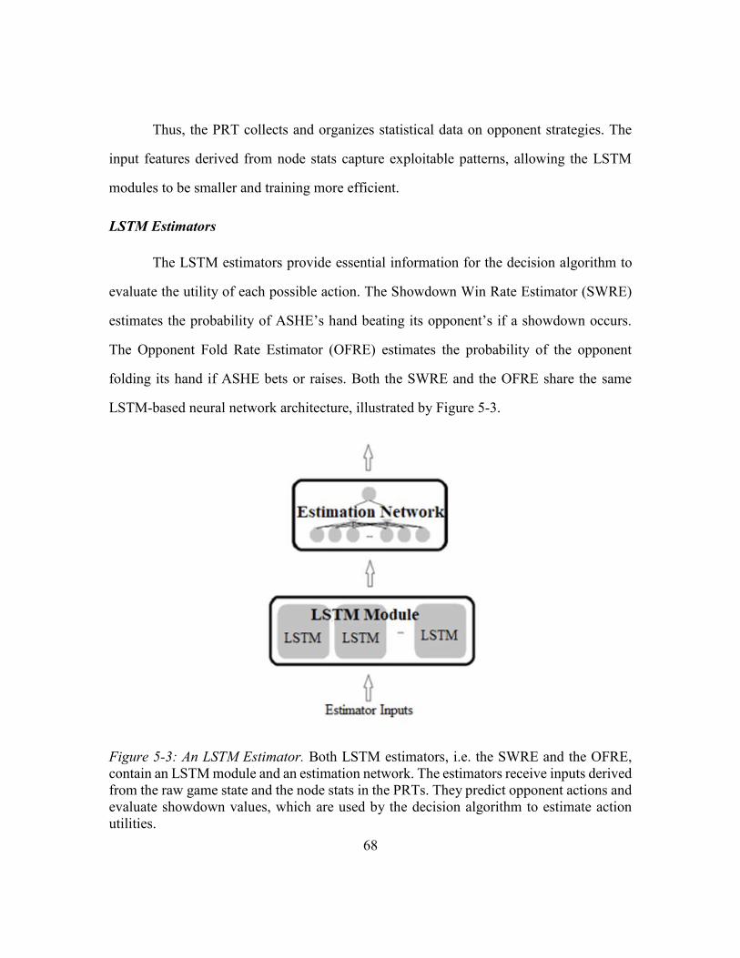
68

Thus, the PRT collects and organizes statistical data on opponent strategies. The

input features derived from node stats capture exploitable patterns, allowing the LSTM

modules to be smaller and training more efficient.

LSTM Estimators

The LSTM estimators provide essential information for the decision algorithm to

evaluate the utility of each possible action. The Showdown Win Rate Estimator (SWRE)

estimates the probability of ASHE’s hand beating its opponent’s if a showdown occurs.

The Opponent Fold Rate Estimator (OFRE) estimates the probability of the opponent

folding its hand if ASHE bets or raises. Both the SWRE and the OFRE share the same

LSTM-based neural network architecture, illustrated by Figure 5-3.

Figure 5-3: An LSTM Estimator. Both LSTM estimators, i.e. the SWRE and the OFRE,

contain an LSTM module and an estimation network. The estimators receive inputs derived

from the raw game state and the node stats in the PRTs. They predict opponent actions and

evaluate showdown values, which are used by the decision algorithm to estimate action

utilities.

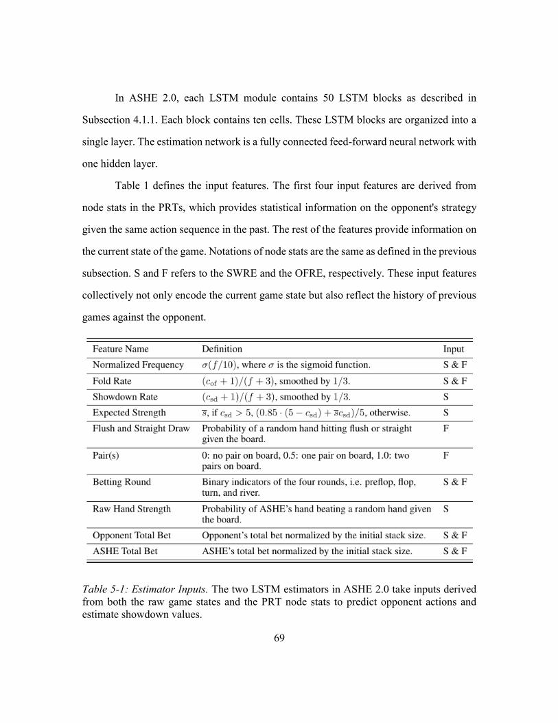
69

In ASHE 2.0, each LSTM module contains 50 LSTM blocks as described in

Subsection 4.1.1. Each block contains ten cells. These LSTM blocks are organized into a

single layer. The estimation network is a fully connected feed-forward neural network with

one hidden layer.

Table 1 defines the input features. The first four input features are derived from

node stats in the PRTs, which provides statistical information on the opponent's strategy

given the same action sequence in the past. The rest of the features provide information on

the current state of the game. Notations of node stats are the same as defined in the previous

subsection. S and F refers to the SWRE and the OFRE, respectively. These input features

collectively not only encode the current game state but also reflect the history of previous

games against the opponent.

Table 5-1: Estimator Inputs. The two LSTM estimators in ASHE 2.0 take inputs derived

from both the raw game states and the PRT node stats to predict opponent actions and

estimate showdown values.

70

At the beginning of each hand, all LSTM blocks in the estimators are set to their

initial states. Suppose ASHE plays the button and needs to decide its first action preflop.

The features in Table 5-1 will be derived from the raw game state and the node stats in the

current PRT node (in this case, the root of the tree). After the input features are sent to the

LSTM modules in both estimators, the states of the LSTM modules will be saved as the

current states. Note that if the node does not exist or the node stats are not reliable, the

default inputs will be used instead.

The output of the SWRE based on the current states will be sent to the decision

algorithm to estimate the utility for every possible action, including fold, check/call, and

bet/raise. ASHE assumes that the opponent will never fold when check is available.

Therefore, the probability of the opponent folding its hand after a check or call is always

assumed to be zero. However, for a bet/raise, the probability of inducing a fold from the

opponent, a.k.a. the fold equity, is crucial for estimating the utility.

To compute the fold equity, the system need to look one step ahead by assuming

that ASHE makes a bet/raise of a certain size. Input features will be computed using the

node stats that correspond to the action. After receiving the input features and predicting

the fold equity for the bet/raise, the OFRE will be reset to the current states. Fold equity

prediction will be made for bets/raises of all legitimate sizes.

As the game proceeds, input features derived from the raw game states and the node

stats corresponding to each action will be sent to the LSTM estimators. Thus, the estimators

can make predictions based on every move in this hand as well as the patterns that are

captured in previous games with similar situation.

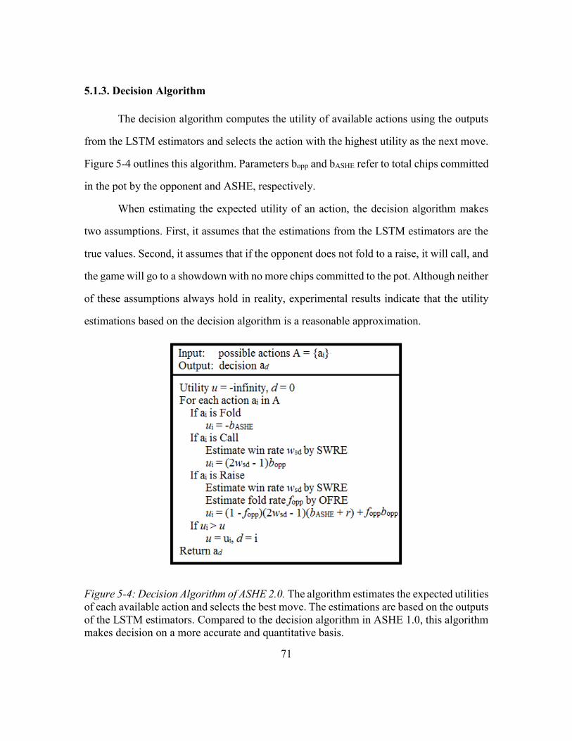
71

5.1.3. Decision Algorithm

The decision algorithm computes the utility of available actions using the outputs

from the LSTM estimators and selects the action with the highest utility as the next move.

Figure 5-4 outlines this algorithm. Parameters bopp and bASHE refer to total chips committed

in the pot by the opponent and ASHE, respectively.

When estimating the expected utility of an action, the decision algorithm makes

two assumptions. First, it assumes that the estimations from the LSTM estimators are the

true values. Second, it assumes that if the opponent does not fold to a raise, it will call, and

the game will go to a showdown with no more chips committed to the pot. Although neither

of these assumptions always hold in reality, experimental results indicate that the utility

estimations based on the decision algorithm is a reasonable approximation.

Figure 5-4: Decision Algorithm of ASHE 2.0. The algorithm estimates the expected utilities

of each available action and selects the best move. The estimations are based on the outputs

of the LSTM estimators. Compared to the decision algorithm in ASHE 1.0, this algorithm

makes decision on a more accurate and quantitative basis.

72

In addition, a restriction is placed on ASHE’s actions: when facing a four-bet (as

the Big Blind) or a three-bet (as the Button) ASHE can only respond with a fold, a call, or

an all-in. This restriction simplifies utility estimation and reduces the size of the PRTs.

In sum, the ASHE 2.0 architecture uses the PRTs to collect statistical information

on the opponent’s moves given different at decision points. The LSTM estimators consider

such information and the game state at each decision point in the current hand to estimate

ASHE’s winning probability in a showdown and the probability of the opponent folding to

bets/raises. The decision algorithm uses these outputs to approximate the expected utility

of available actions and selects the best move accordingly.

Evolving high-performance computer agents for large-scale imperfect information

games is a challenging task. The ASHE 2.0 architecture provides a structural framework

for building such agents and should be applicable to domains other than poker as well.

5.2. EVOLUTION OF THE LSTM ESTIMATORS

The performance of ASHE depends on the accuracy of the LSTM estimators.

Although it is clear what the LSTM estimators need to do, how can they be trained to do

it? As is discussed in Subsection 4.2.1, it is difficult to obtain sufficient labeled data for

training adaptive poker agents. In fact, even the definition of “correctness” is unclear. For

example, what is the chance of the opponent folding to a half-pot raise given the current

game state and the history of previous games? While most professional human players may

be able to figure out a reasonable range, it is impossible to give an answer that is correct in

an absolute sense.

Therefore, the LSTM estimators cannot be trained through supervised methods. A

major technical insight in this work is that it is possible to evolve the LSTM estimators for

73

their tasks with genetic algorithms as outlined in Section 4.2. This approach makes the

method applicable to problems with little or no labeled training data.

In the genetic algorithm, a population of agents are created with randomly

initialized LSTM estimators at first. They are evaluated based on their fitness, i.e. their

performance against a variety of training opponents. These opponents require different

counter-strategies for effective exploitation. Thus, the agents with adaptive behaviors that

can exploit various strategies are rewarded by higher fitness. The agents with the highest

fitness survive and reproduce via mutation and crossover. The others are replaced by the

offspring. Selection and reproduction are done iteratively, thus improving the overall

fitness of the population. Note that the agents do not have to know what the accurate

estimations are or what actions are the best; it is sufficient to select agents that perform

relatively well in the population.

Specifically, during evolution, agents are represented by theirs numeric genomes,

which are constructed by concatenating all parameters in the estimators, i.e. the weights in

the LSTM module, the initial states of all LSTM blocks, and the weights of the estimation

network.

To preserve advantageous genotypes against occasional poor luck, Tiered Survival

and Elite Reproduction (TSER, as introduced in Section 4.2.2) is adopted. Survivors are

divided into two tiers based on their fitness. Agents in the top tier (i.e. the elite tier), can

reproduce and do not mutate. Agents of the second tier mutate but cannot reproduce. Thus,

genotypes from more agents can be preserved without compromising the performance of

the offspring.

Evolving agents with multiple modules can be inefficient, especially at an early

stage. Advantageous genotypes of one module may be coupled with poor genotypes of

another, causing low performance and loss of progress. Therefore, evolution is organized

74

into a series of sessions, with each session dedicated to evolving one of the estimators.

When a new session begins, the champion of the previous session is duplicated to form the

agent population. The weights in the estimator to be evolved are mutated, and the weights

in the other estimator frozen. Thus, the genetic algorithm is able to discover effective

LSTM estimators efficiently, although there is no data for supervised training.


ASHE 2.0 agents were evolved by playing against opponents with different level

of exploitability. A total of 11 agents were used to evaluate ASHE’s performance against

both weak and strong opponents.

Below, Subsection 5.3.1 provides details on the experimental setup and match

formats, Subsection 5.3.2 introduces the opponents in training and testing, and Subsection

5.3.3 presents and discusses the results.


Table 5-2 presents the parameters in the experiments. During training, evolution

was organized into sessions. Each session evolves one of the two LSTM modules, i.e. the

OFRE or the SWRE, and freezes the other (Subsection 5.2). The champions of the last

generation were used for evaluation.

Mutation followed Gaussian distribution. As evolution proceeded, mutation rate

and mutation strength (i.e. the standard deviation of the Gaussian distribution) descended

linearly. Similar to the ASHE 1.0 experiments, fitness was measured by the Average

Normalized Earnings (ANE, as in Subsection 4.3.3). Survivors whose fitness was higher

than the mean of fitness among all survivors became the elites in TSER.

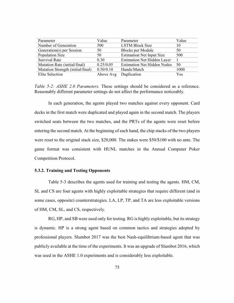
75

Table 5-2: ASHE 2.0 Parameters. These settings should be considered as a reference.

Reasonably different parameter settings do not affect the performance noticeably.

In each generation, the agents played two matches against every opponent. Card

decks in the first match were duplicated and played again in the second match. The players

switched seats between the two matches, and the PRTs of the agents were reset before

entering the second match. At the beginning of each hand, the chip stacks of the two players

were reset to the original stack size, $20,000. The stakes were $50/$100 with no ante. The

game format was consistent with HUNL matches in the Annual Computer Poker

Competition Protocol.

5.3.2. Training and Testing Opponents

Table 5-3 describes the agents used for training and testing the agents. HM, CM,

SL and CS are four agents with highly exploitable strategies that require different (and in

some cases, opposite) counterstrategies. LA, LP, TP, and TA are less exploitable versions

of HM, CM, SL, and CS, respectively.

RG, HP, and SB were used only for testing. RG is highly exploitable, but its strategy

is dynamic. HP is a strong agent based on common tactics and strategies adopted by

professional players. Slumbot 2017 was the best Nash-equilibrium-based agent that was

publicly available at the time of the experiments. It was an upgrade of Slumbot 2016, which

was used in the ASHE 1.0 experiments and is considerably less exploitable.

Parameter Value Parameter Value

Number of Generation 500 LSTM Block Size 10

Generation(s) per Session 50 Blocks per Module 50

Population Size 50 Estimation Net Input Size 500

Survival Rate 0.30 Estimation Net Hidden Layer 1 Mutation Rate (initial/final) 0.25/0.05 Estimation Net Hidden Nodes 50 Mutation Strength (initial/final) 0.50/0.10 Hands/Match 1000

Elite Selection Above Avg Duplication Yes

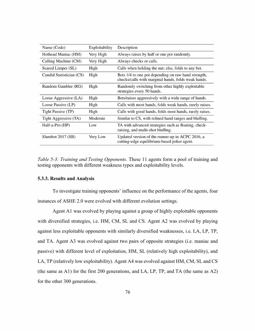
76

Table 5-3: Training and Testing Opponents. These 11 agents form a pool of training and

testing opponents with different weakness types and exploitability levels.

5.3.3. Results and Analysis

To investigate training opponents’ influence on the performance of the agents, four

instances of ASHE 2.0 were evolved with different evolution settings.

Agent A1 was evolved by playing against a group of highly exploitable opponents

with diversified strategies, i.e. HM, CM, SL and CS. Agent A2 was evolved by playing

against less exploitable opponents with similarly diversified weaknesses, i.e. LA, LP, TP,

and TA. Agent A3 was evolved against two pairs of opposite strategies (i.e. maniac and

passive) with different level of exploitation, HM, SL (relatively high exploitability), and

LA, TP (relatively low exploitability). Agent A4 was evolved against HM, CM, SL and CS

(the same as A1) for the first 200 generations, and LA, LP, TP, and TA (the same as A2)

for the other 300 generations.

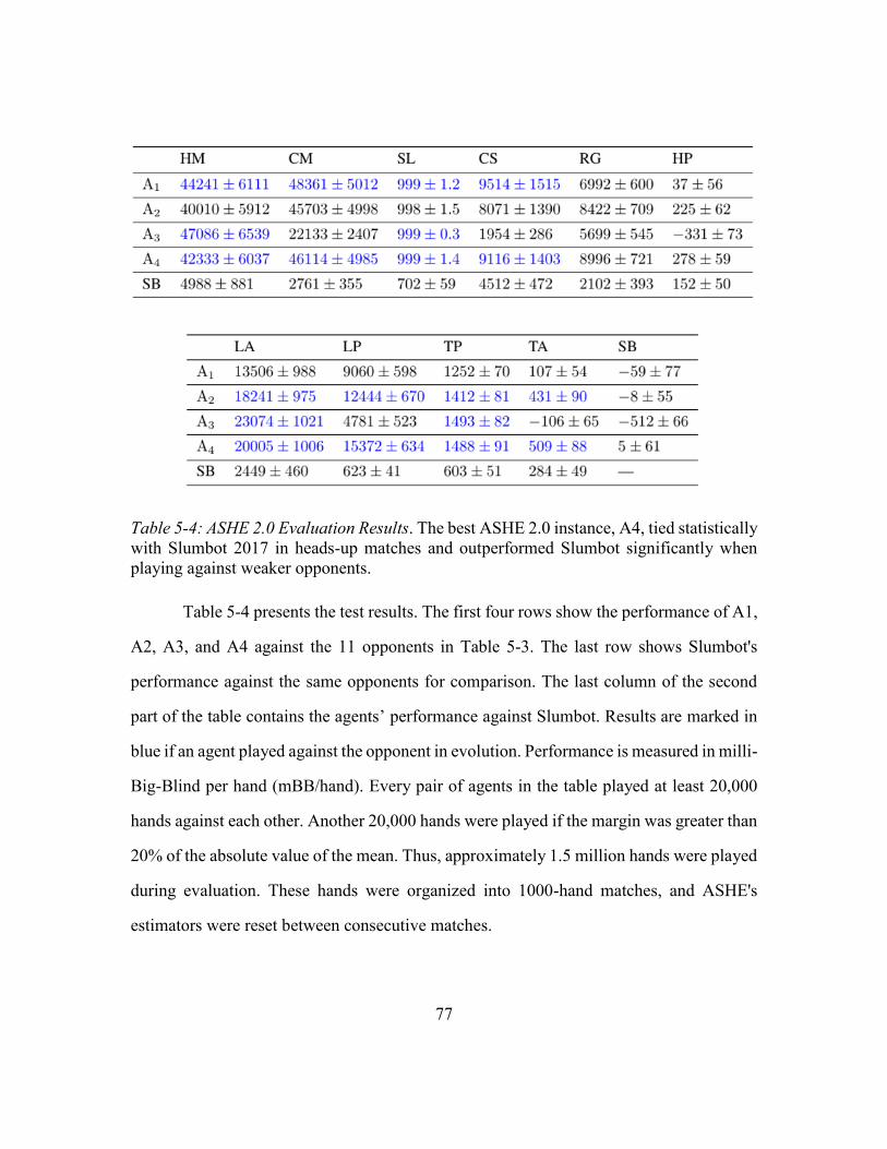
77

Table 5-4: ASHE 2.0 Evaluation Results. The best ASHE 2.0 instance, A4, tied statistically

with Slumbot 2017 in heads-up matches and outperformed Slumbot significantly when

playing against weaker opponents.

Table 5-4 presents the test results. The first four rows show the performance of A1,

A2, A3, and A4 against the 11 opponents in Table 5-3. The last row shows Slumbot's

performance against the same opponents for comparison. The last column of the second

part of the table contains the agents’ performance against Slumbot. Results are marked in

blue if an agent played against the opponent in evolution. Performance is measured in milli-

Big-Blind per hand (mBB/hand). Every pair of agents in the table played at least 20,000

hands against each other. Another 20,000 hands were played if the margin was greater than

20% of the absolute value of the mean. Thus, approximately 1.5 million hands were played

during evaluation. These hands were organized into 1000-hand matches, and ASHE's

estimators were reset between consecutive matches.

78

Overall, the best of the four ASHE 2.0 instances is A4, followed by A2, A1, and

A3 in decreasing order of their average performance. A1 through A3 were mainly used as

control group agents.

Performance vs. High-exploitability Opponents

The results show that ASHE 2.0 is remarkably effective in exploiting weak

opponents. Opponent modeling and adaptation allow the agents to quickly adjust their

strategies and take advantage of the opponent’s weaknesses. In the experiments, eight

opponents were considered highly exploitable: HM, SL, CM, CS, LP, TP and RG. These

agents are theoretically highly exploitable because their strategies are flawed. However, to

exploit their weaknesses effectively, an agent must adopt different counter-strategies that

may require entirely opposite actions facing similar game states. Thus, these highly

exploitable agents form an effective test group for opponent modeling and adaptation.

As is shown in Table 5-4, the best instance, A4, outperformed SB 40% to 2300%

when playing against the highly exploitable opponents. The performance gap depends on

the type of the weaknesses and the level of exploitability. Generally, the more exploitable

the opponent strategy is, the bigger the margin tends to be. Furthermore, the second-best

instance, A2, evolved by playing against LA, LP, TP, and TA, was much more effective

than SB when facing HM, CM, SL and CS. These results show that ASHE’s performance

advantage over Nash-equilibrium-based agents is not limited to opponents seen during

training. Therefore, the proposed method can build poker agents that are significantly more

effective in exploiting weak opponents than top-ranking agents following equilibrium-

based strategies.

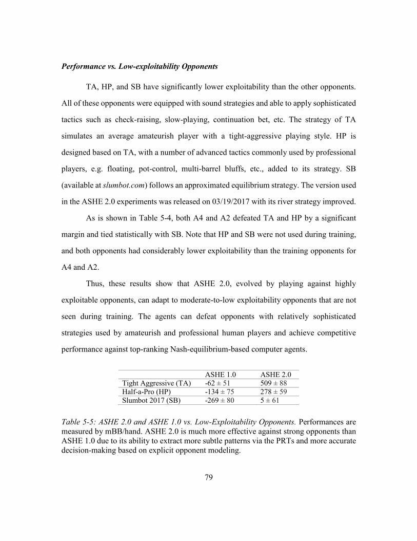
79

Performance vs. Low-exploitability Opponents

TA, HP, and SB have significantly lower exploitability than the other opponents.

All of these opponents were equipped with sound strategies and able to apply sophisticated

tactics such as check-raising, slow-playing, continuation bet, etc. The strategy of TA

simulates an average amateurish player with a tight-aggressive playing style. HP is

designed based on TA, with a number of advanced tactics commonly used by professional

players, e.g. floating, pot-control, multi-barrel bluffs, etc., added to its strategy. SB

(available at slumbot.com) follows an approximated equilibrium strategy. The version used

in the ASHE 2.0 experiments was released on 03/19/2017 with its river strategy improved.

As is shown in Table 5-4, both A4 and A2 defeated TA and HP by a significant

margin and tied statistically with SB. Note that HP and SB were not used during training,

and both opponents had considerably lower exploitability than the training opponents for

A4 and A2.

Thus, these results show that ASHE 2.0, evolved by playing against highly

exploitable opponents, can adapt to moderate-to-low exploitability opponents that are not

seen during training. The agents can defeat opponents with relatively sophisticated

strategies used by amateurish and professional human players and achieve competitive

performance against top-ranking Nash-equilibrium-based computer agents.

ASHE 1.0 ASHE 2.0 Tight Aggressive (TA) -62 ± 51 509 ± 88

Half-a-Pro (HP) -134 ± 75 278 ± 59

Slumbot 2017 (SB) -269 ± 80 5 ± 61

Table 5-5: ASHE 2.0 and ASHE 1.0 vs. Low-Exploitability Opponents. Performances are

measured by mBB/hand. ASHE 2.0 is much more effective against strong opponents than

ASHE 1.0 due to its ability to extract more subtle patterns via the PRTs and more accurate

decision-making based on explicit opponent modeling.

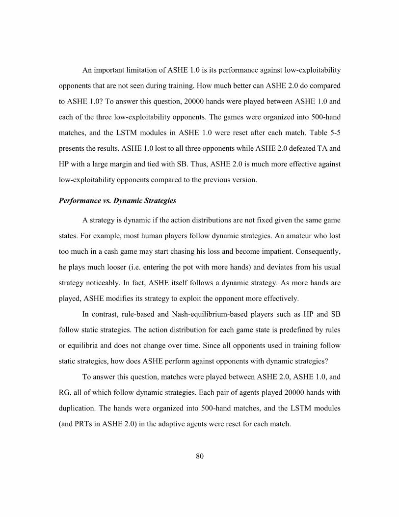
80

An important limitation of ASHE 1.0 is its performance against low-exploitability

opponents that are not seen during training. How much better can ASHE 2.0 do compared

to ASHE 1.0? To answer this question, 20000 hands were played between ASHE 1.0 and

each of the three low-exploitability opponents. The games were organized into 500-hand

matches, and the LSTM modules in ASHE 1.0 were reset after each match. Table 5-5

presents the results. ASHE 1.0 lost to all three opponents while ASHE 2.0 defeated TA and

HP with a large margin and tied with SB. Thus, ASHE 2.0 is much more effective against

low-exploitability opponents compared to the previous version.

Performance vs. Dynamic Strategies

A strategy is dynamic if the action distributions are not fixed given the same game

states. For example, most human players follow dynamic strategies. An amateur who lost

too much in a cash game may start chasing his loss and become impatient. Consequently,

he plays much looser (i.e. entering the pot with more hands) and deviates from his usual

strategy noticeably. In fact, ASHE itself follows a dynamic strategy. As more hands are

played, ASHE modifies its strategy to exploit the opponent more effectively.

In contrast, rule-based and Nash-equilibrium-based players such as HP and SB

follow static strategies. The action distribution for each game state is predefined by rules

or equilibria and does not change over time. Since all opponents used in training follow

static strategies, how does ASHE perform against opponents with dynamic strategies?

To answer this question, matches were played between ASHE 2.0, ASHE 1.0, and

RG, all of which follow dynamic strategies. Each pair of agents played 20000 hands with

duplication. The hands were organized into 500-hand matches, and the LSTM modules

(and PRTs in ASHE 2.0) in the adaptive agents were reset for each match.

81

Table 5-6: Performance of ASHE against Dynamic Strategies. Green, yellow, and red

indicate the agent in the row winning, tying, and losing against the agent in the column

with a 0.95 confidence, respectively. ASHE 2.0 exploits dynamic strategies more

effectively than SB does. Both ASHE 2.0 and ASHE 1.0 defeats highly exploitable

dynamic strategies, e.g. RG, with a big margin.

Table 5-6 presents the results. Performance of SB against each agent is provided

for comparison. Both ASHE 2.0 and ASHE 1.0 were more effective in exploiting RG than

SB. In addition, ASHE 2.0 defeated ASHE 1.0 with a much bigger margin than SB did.

These results show that ASHE 2.0 can adapt to dynamic strategies and exploit them more

effectively than equilibrium-based agents. The performance gap tends to get bigger with

more exploitable opponents.

To understand how ASHE 2.0 adapts to dynamic strategies, snapshots of ASHE’s

strategy were taken after every 50 hands in a 500-hand match against RG. Each snapshot

strategy was evaluated against RG and the strategy RG chose in the previous 50 hands

before the snapshot was taken.

In the sample shown by Table 5-7, RG chose the SL strategy during the first 50

hands. The snapshot strategy at hand 50 achieved maximum performance against SL.

However, when facing RG, it did not perform better than SB did. As more hands were

played, ASHE’s performance against RG improved rapidly. By the end of hand 200, ASHE

had played against each strategy RG might choose for at least 50 hands. The performance

of the snapshot strategy at hand 250 is four times better than that of SB against RG. The

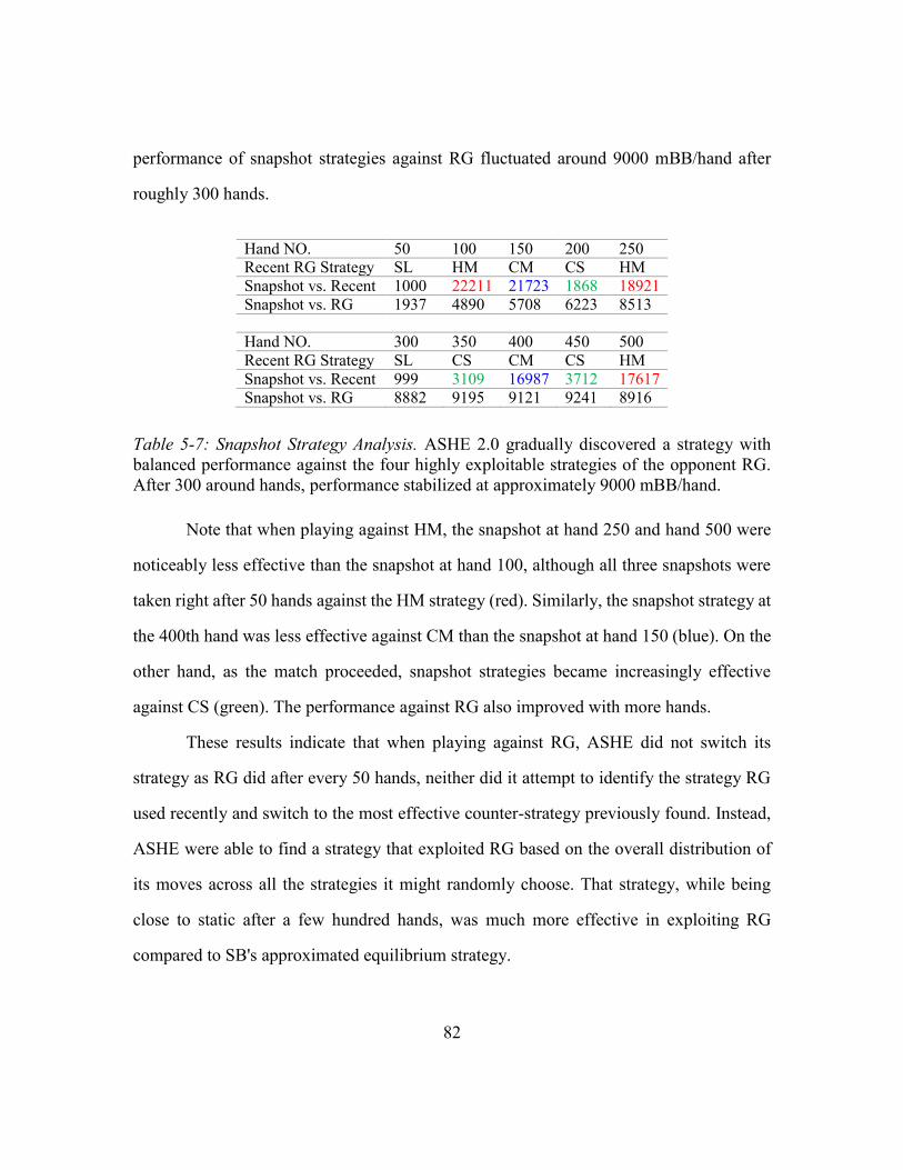
82

performance of snapshot strategies against RG fluctuated around 9000 mBB/hand after

roughly 300 hands.

Hand NO. 50 100 150 200 250 Recent RG Strategy SL HM CM CS HM

Snapshot vs. Recent 1000 22211 21723 1868 18921

Snapshot vs. RG 1937 4890 5708 6223 8513

Hand NO. 300 350 400 450 500

Recent RG Strategy SL CS CM CS HM

Snapshot vs. Recent 999 3109 16987 3712 17617

Snapshot vs. RG 8882 9195 9121 9241 8916

Table 5-7: Snapshot Strategy Analysis. ASHE 2.0 gradually discovered a strategy with

balanced performance against the four highly exploitable strategies of the opponent RG.

After 300 around hands, performance stabilized at approximately 9000 mBB/hand.

Note that when playing against HM, the snapshot at hand 250 and hand 500 were

noticeably less effective than the snapshot at hand 100, although all three snapshots were

taken right after 50 hands against the HM strategy (red). Similarly, the snapshot strategy at

the 400th hand was less effective against CM than the snapshot at hand 150 (blue). On the

other hand, as the match proceeded, snapshot strategies became increasingly effective

against CS (green). The performance against RG also improved with more hands.

These results indicate that when playing against RG, ASHE did not switch its

strategy as RG did after every 50 hands, neither did it attempt to identify the strategy RG

used recently and switch to the most effective counter-strategy previously found. Instead,

ASHE were able to find a strategy that exploited RG based on the overall distribution of

its moves across all the strategies it might randomly choose. That strategy, while being

close to static after a few hundred hands, was much more effective in exploiting RG

compared to SB's approximated equilibrium strategy.

83

Adaptation in matches between ASHE 2.0 and ASHE 1.0 appeared to be similar.

At the beginning, the two adaptive agents changed their behaviors drastically, racing for a

strategy to better exploit the opponent. As more hands were played, the strategies of both

agents started converging. After a few hundred hands, the performance became stable.

Thus, ASHE 2.0 adapts to dynamic strategies by reacting to their overall action

distribution rather than just following the recent moves.

Training Opponent(s) and Performance

Results in Table 5-4 also provide insights into how opponents should be selected

and arranged for training/evolution. First, the performance of A3 was much worse than the

other three instances when facing opponents whose strategies were fundamentally different

from those seen during evolution. For instance, CM and CS are fundamentally different

from any opponent used in A3’s training. Consequently, A3’s performance against these

agents were much lower than that of A1, A2, or A4. Moreover, A3’s strategy did not

perform well against stronger opponents that were not seen during training. In contrast,

instances evolved by playing against a reasonably diversified set of strategies, e.g. A1, A2,

and A4, could adapt to HP or SL, whose strategies were superior to any strategies seen

during evolution.

These results indicate that a reasonable level of diversity of opponent strategies

during evolution is necessary for evolving strong adaptive agents. It is unlikely for an agent

that has never seen maniac-style bluffing to exploit it effectively. In other words, the agents

should be exposed to different types of weaknesses through evolution. With such diversity,

however, agents can generalize remarkably well to opponents that are not seen in training.

While exploitable patterns can be categorized into many types, agents with these

patterns may have different level of exploitability. For example, TP and SL both tend to

84

underestimate the value of their hands and fold more often than they should. However, SL

is extremely cautious and only plays the absolute best hands, and TP continues with a

noticeably wider range. Suppose multiple agents with the same type of weaknesses are

available for training, which works better as a training opponent?

In the experiments, A2 and A1 were evolved by playing against opponents with the

same types of weakness. A2’s training opponents, i.e. LA, LP, TP, and TA, were less

exploitable compared to A1’s training opponents, i.e. HM, SL, CM, and CS. As a result,

A2 achieved consistently better performance than A1 when playing against opponents that

had not been seen during evolution. Therefore, the level of exploitability of opponent

strategies during evolution is another factor that influences performance. Moderately

exploitable opponents tend to be more effective as training opponents than a highly

exploitable opponents with similar types of weakness.

Experimental results also indicate that combining training opponents with high and

low level of exploitability can improve performance. In particular, highly exploitable

training opponents can be used in early generations. Once the agents start demonstrating

adaptive behaviors, less exploitable training opponents can be introduced. For instance,

both A2 and A4 played against LA, LP, TP, and TA during training. Nevertheless, A4 were

evolved by first playing against a group of more exploitable opponents with similar types

of weakness, i.e. HM, SL, CM and CS. In matches against opponents that were not seen

by both agents during training, A4 performed consistently better than A2.

In addition, using highly exploitable agents at the early stage of evolution can

improve training efficiency, because they are more sensitive to exploitation and provide

more incentive for the agents to explore adaptive behaviors. In comparison, exploitable

patterns of stronger opponents tend to be more subtle and offer less reward even if fully

85

exploited. These subtle patterns are great training examples after enough generations, but

may be overwhelming for the agent population in the beginning.

The above observations and findings show that the proposed approach is effective

in building high-quality adaptive agents for HUNL. They also provide useful principles for

its application and improvement in the future.

5.4. DISCUSSION AND CONCLUSION

ASHE 2.0 introduces two major improvements to the previous version: (1) Pattern

Recognition Trees/PRTs and (2) explicit opponent modeling. The PRTs are tree structures

whose nodes correspond to the game states. They collect statistical data on the opponent’s

strategy and serve as a feature extractor of the opponent model. Input features derived from

the node stats in PRT are sent to the LSTM modules, which evaluate fold equities and

showdown values. The PRTs improve performance in two ways. First, they extract useful

features on the opponent’s strategy from the game history. Second, they reduce the

complexity of the task for the LSTM modules, thus allowing the networks to be smaller

and evolution more efficient.

Explicit opponent modeling refers to predicting opponent actions, estimating hand

strength, etc. These predictions can be used to estimate the utility of each possible action,

providing a more accurate method for deciding the next moves. ASHE 2.0 evaluates fold

equity and showdown value with LSTM modules, which take inputs derived from raw

game states and the PRT node stats.

Experimental results demonstrates that ASHE 2.0 is significantly more effective

than cutting-edge equilibrium-based agents in exploiting weak opponents. In addition,

ASHE 2.0 can adapt to opponents that are not seen during training, even if they are much

stronger than the training opponents. In particular, ASHE 2.0 tied statistically in heads-up

86

matches with Slumbot 2017, an upgrade of the equilibrium-based agent used in the ASHE

1.0 experiments. The PRT-LSTM-based opponent model is effective in matches against

both static and dynamic strategies. Experimental results show that ASHE 2.0 outperforms

Slumbot by significant margin facing dynamic opponents with different level of

exploitability.

Empirical results also provide insights into how opponents should be selected and

arranged during evolution. Training opponent should be reasonably diversified to ensure

generalizability. Moderately exploitable opponents in training tend to yield better results

than highly exploitable opponents with similar types of weakness. Nevertheless, highly

exploitable opponents can be used in early generations to encourage adaptive behaviors.

While ASHE 2.0 achieved much higher performance than the previous version

against strong opponents that are not seen during training, it can be further improved in

several ways. Chapter 6 to 8 introduce various extensions of ASHE 2.0 and investigate

their influence on performance. Chapter 6 focuses on the PRTs, Chapter 7 focuses on action

utility estimation, and Chapter 8 introduces the Hand Range Estimators. The overall result

will be a version of ASHE that will defeat a wide range of opponents, including Slumbot

2017, in heads-up matches.

87

Chapter 6: Advanced PRT

In ASHE 2.0, the Pattern Recognition Tree serves as a feature extractor for the

opponent model and plays an important role in capturing exploitable patterns in the

opponent’s strategy. However, the PRTs in ASHE 2.0 have two limitations: (1) they cannot

provide useful node stats when facing a new opponent or an infrequent game state, and (2)

they do not take community cards into consideration.

This chapter introduces advanced PRTs, which addresses the above limitations.

Advance PRT entails two techniques: the default PRT (Section 6.1), which models the

actions of an unknown opponent, and the board-texture-based PRT (Section 6.2), which is

able to capture exploitable patterns based on the community cards. Section 6.3 presents

and analyzes experimental results on ASHE 2.1, the upgraded version with advanced PRT.

6.1. DEFAULT PRT

The default PRT allows the agents to make better decisions in the early stage of a

match when node stats are unreliable, thus improving overall performance. This technique

is also a prerequisite for the PRTs to model the opponents based on board textures, because

collecting reliable node stats on such specific game states takes more hands, and decision

quality must be guaranteed before node stats become reliable.

6.1.1. Motivation

The PRTs in ASHE 2.0 are updated in a lazy fashion. They are initialized with a

root node that represents one of the two initial states of the game. Nodes representing the

other game states are inserted to the PRTs when the game states occur in the match. Even

if the node corresponding to a game state already exists in the PRTs, node stats cannot be

used to derive inputs for the LSTM estimators before the game state occurs enough times

88

to generate meaningful data. Thus, in the early stage of a match, the agent have to make

many decisions essentially without the support of the PRTs.

In ASHE 2.0, if node stats are not reliable, a set of default values are sent to the

estimators in place of the features derived from the node stats. Different default values are

selected for each betting round. These values are estimated based on domain knowledge

and empirical results. They do not provide information on the opponent’s strategy, neither

do they correspond to any specific game state. Consequently, ASHE’s strategy in the early

stage of a match, i.e. the first 50 to 100 hands, tends to be unstable and flawed, reducing

overall performance.

Moreover, the more nodes the PRTs have, the longer it takes to collect reliable node

stats. Hence, the low quality of default values makes it infeasible to expand the PRTs to

represent more specific game states. In fact, it is the main reason for the PRT nodes in

ASHE 2.0 to ignore the community cards.

The key to address the above problem is to provide high quality default inputs for

the LSTM estimators when node stats are unreliable. While it is impossible to extract

exploitable patterns in a specific strategy without sufficient observation, a player can still

make good decisions in the early stage of a match.

When facing a new opponent at the table, a human player usually adopts an initial

strategy based on his/her experience from games against other players. As more hands are

played, the player learns about the opponent and adapts his/her strategy accordingly.

Similarly, default inputs for the LSTM estimators can be generated from games played

against other opponents. Such inputs may not represent the strategy of the current

opponent. However, they allow the agent to make decisions at infrequent states that work

well enough against most opponents.

89

Default PRT is designed to provide such inputs. It is used in combination with the

opponent-specific PRTs introduced in Chapter 5, allowing the agents to make good early-

match decisions. The next subsection details this technique.

6.1.2. Construction and Application

A default PRT has the same structure as the regular PRT and maintains the same

set of node stats listed in Subsection 5.1.2. However, they represent different strategies.

The regular PRTs are built for each opponent from scratch. As more hands are

played, the regular PRTs grow, and the node stats become increasingly reliable. They

reflect the strategy of the current opponent. In contrast, the default PRTs are built during

training. They do not change in a match, and their node stats are used to derive input

features for the LSTM estimators when the regular PRTs cannot provide reliable node stats.

The default PRTs represent the general strategy ASHE adopts when facing a new opponent

or game state.

Construction

Like the regular PRTs, the default PRTs are constructed through playing against

other agents. When evolving agents with default PRTs, each generation is divided into two

sessions: a preliminary session and an evaluation session.

In the preliminary session, the agents play against the default opponent(s). The

entire session is treated as one match, and the PRTs are not reset even if the agents play

against multiple opponents. Default values are used when facing new game states like the

ASHE 2.0 baseline. At the end of the session, the PRTs are saved as the default PRTs.In

the evaluation session, the agents play against their opponents using both the default PRTs

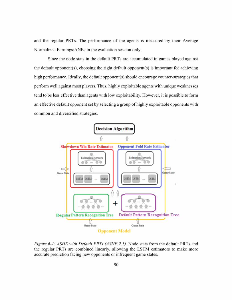
90

and the regular PRTs. The performance of the agents is measured by their Average

Normalized Earnings/ANEs in the evaluation session only.

Since the node stats in the default PRTs are accumulated in games played against

the default opponent(s), choosing the right default opponent(s) is important for achieving

high performance. Ideally, the default opponent(s) should encourage counter-strategies that

perform well against most players. Thus, highly exploitable agents with unique weaknesses

tend to be less effective than agents with low exploitability. However, it is possible to form

an effective default opponent set by selecting a group of highly exploitable opponents with

common and diversified strategies.

Figure 6-1: ASHE with Default PRTs (ASHE 2.1). Node stats from the default PRTs and

the regular PRTs are combined linearly, allowing the LSTM estimators to make more

accurate prediction facing new opponents or infrequent game states.

91

Application

Figure 6-1 presents the architecture of ASHE 2.1, an upgrade of the baseline

equipped with the default PRTs. The game states are sent to the default PRTs for tracking

actions in the game and retrieving node stats. Unlike the regular ones, the default PRTs are

not updated at the end of each hand. Given a game state, the node stats are retrieved from

each of the two PRTs. The stats are linearly combined based on the state frequency f (as

defined in Subsection 5.1.2) and the normalization factor λ:

𝑣 = { 𝑓

λ𝑣R + (1 −

𝑓

λ) 𝑣D (𝑓 < λ)

𝑣R (𝑓 ≥ λ) ,

where v is the node stats value used to derive input features for the LSTM estimators, vR

and vD are the node stats from the regular PRT and the default PRT, respectively. The

normalization factor λ can be adjusted based on the depth of the nodes. The deeper the

nodes are, the more difficult it is for the regular PRTs to collect reliable data. Hence, λ can

be smaller for deeper nodes.

If the node stats in the default PRT is also unreliable, the default features are sent

to the LSTM estimators. However, such cases are extremely rare and do not influence

overall performance.

Thus, the default PRTs provide node stats representing the default opponent(s) to

derive input features for the LSTM estimators. They allow the estimators to make reliable

predictions even if ASHE has little information on the opponent.

6.2. BOARD-TEXTURE-BASED PRT

With the default PRTs in place, the LSTM estimators no longer rely solely on the

regular PRT node stats for inputs features. Therefore, the regular PRTs are allowed more

92

time to collect reliable node stats. This means the PRT nodes can represent more specific

game states and capture more subtle patterns in the opponent strategies.

This section introduces board-texture-based PRT, which maintains node stats for

game states defined by the action sequence and the patterns in the community cards. The

board-texture-based PRT and the default PRT technique are applied together to build the

advanced PRTs in ASHE 2.1.

6.2.1. Motivation

The raw game state of HUNL is defined by the action sequence, the private cards,

and the community cards. The nodes of the PRTs in ASHE 2.0 only represent the action

sequences. What should be added to make the PRT more effective for opponent modeling

and exploitation?

The private cards certainly play an important role in the game. Nevertheless, they

are not a viable option to be represented by the PRT nodes. The opponent strategy is not

related to ASHE’s private cards. The opponent makes decisions based on its own private

cards, the action sequence, and the community cards. Knowing the opponent’s private

cards is very helpful in modeling the opponent strategy. However, a large portion of hands

end without a showdown, and the opponent’s private cards are never revealed. Hence, it is

difficult to extract or update the node stats.

The community cards, a.k.a. the board, is critical for making decisions in HUNL.

Many exploitable patterns may be closely related to the texture of the board. For instance,

some players tend to overvalue flush and/or straight draws and semi-bluff excessively.

Taking the board into consideration is necessary to discover and exploit such weaknesses.

The biggest challenge to introduce the community cards as part of the game states

93

represented by the PRT nodes is the huge number of possible boards. There are over two

million possible boards, and it is impossible to create nodes for all of the combinations.

ASHE 2.1 addresses this problem by clustering the boards at each betting round

based on their texture (e.g. if the board is paired, connected, suited, etc.). Game states are

defined using clusters instead of specific cards. This approach simulates what human

players do. Suppose two cards of the same suit show up on the flop, a human player may

notice that the board allows flush draws, but the specific ranks of the suited cards are often

ignored, unless they are part of another feature that is related to the ranks. Since there are

no more than a dozen of interesting board texture, they can be included in the game state

to represent the community cards. Thus, board-texture-based PRTs are able to capture

patterns that are directly related to the board while collecting reliable node stats quickly.

6.2.2. Implementation

Both the opponent-specific PRTs and default PRTs in ASHE 2.1 are board-texture-

based. This subsection introduces the structure of the board-texture-based PRTs and

specifies the method to generate the board texture clusters.

Board-texture-based PRT Structure

Figure 6-2 illustrates the structure of a board-texture-based PRT. Compared to the

PRTs in ASHE 2.0, the board-texture-based PRTs have one more type of nodes: the board

nodes. Each of them represents a cluster of boards. Since the board nodes are not decision

points, they do not have node stats. The board-texture-based PRTs work in the same way

as the ASHE 2.0 PRTs do, with one exception: when the community cards are dealt, the

board is associated with one of the board texture clusters, and the board node representing

that cluster is visited. If the board node does not exist, one will be added to the tree.

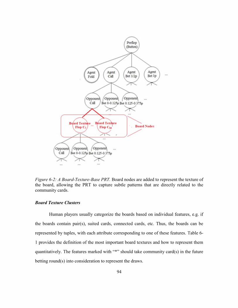
94

Figure 6-2: A Board-Texture-Base PRT. Board nodes are added to represent the texture of

the board, allowing the PRT to capture subtle patterns that are directly related to the

community cards.

Board Texture Clusters

Human players usually categorize the boards based on individual features, e.g. if

the boards contain pair(s), suited cards, connected cards, etc. Thus, the boards can be

represented by tuples, with each attribute corresponding to one of these features. Table 6-

1 provides the definition of the most important board textures and how to represent them

quantitatively. The features marked with “*” should take community card(s) in the future

betting round(s) into consideration to represent the draws.

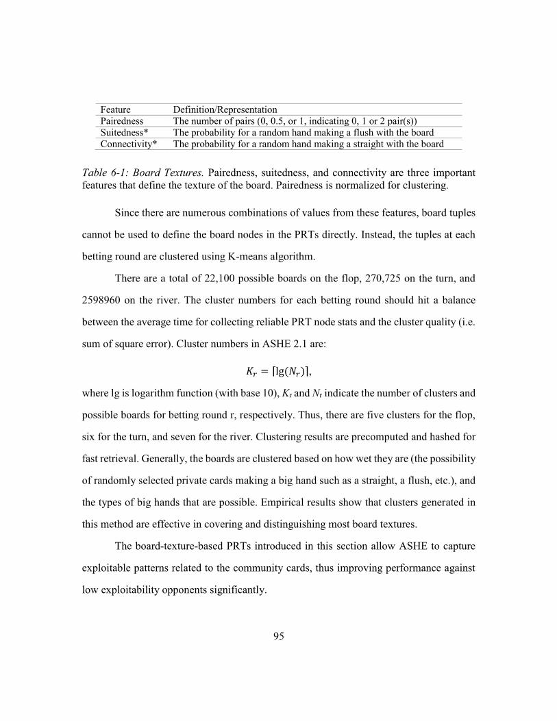
95

Feature Definition/Representation Pairedness The number of pairs (0, 0.5, or 1, indicating 0, 1 or 2 pair(s))

Suitedness* The probability for a random hand making a flush with the board

Connectivity* The probability for a random hand making a straight with the board

Table 6-1: Board Textures. Pairedness, suitedness, and connectivity are three important

features that define the texture of the board. Pairedness is normalized for clustering.

Since there are numerous combinations of values from these features, board tuples

cannot be used to define the board nodes in the PRTs directly. Instead, the tuples at each

betting round are clustered using K-means algorithm.

There are a total of 22,100 possible boards on the flop, 270,725 on the turn, and

2598960 on the river. The cluster numbers for each betting round should hit a balance

between the average time for collecting reliable PRT node stats and the cluster quality (i.e.

sum of square error). Cluster numbers in ASHE 2.1 are:

𝐾𝑟 = ⌈lg (𝑁𝑟)⌉,

where lg is logarithm function (with base 10), Kr and Nr indicate the number of clusters and

possible boards for betting round r, respectively. Thus, there are five clusters for the flop,

six for the turn, and seven for the river. Clustering results are precomputed and hashed for

fast retrieval. Generally, the boards are clustered based on how wet they are (the possibility

of randomly selected private cards making a big hand such as a straight, a flush, etc.), and

the types of big hands that are possible. Empirical results show that clusters generated in

this method are effective in covering and distinguishing most board textures.

The board-texture-based PRTs introduced in this section allow ASHE to capture

exploitable patterns related to the community cards, thus improving performance against

low exploitability opponents significantly.

96


This section presents and analyzes experimental results on ASHE 2.1, which is an

upgrade version of ASHE 2.0 with default PRTs added to the opponent model. Both the

default PRTs and the opponent-specific PRTs in ASHE 2.1 are board-texture-based. For

convenience of discussion, such PRT settings will be referred to as advanced PRT in the

rest of this dissertation.


Although the PRTs are not optimized through evolution, neural network modules

must be re-trained to utilize additional information from the advanced PRTs. Parameters

are set to the same values as in Table 5-2.

The normalization factor λ (as defined in Subsection 6.1.2) should decrease for

nodes representing longer action sequences to keep a balance between node stats from the

default PRTs and the regular PRTs. In the experiments, λ was set to 50, 20, 10, and 5 for

preflop, flop, turn and river nodes, respectively.

The preliminary session for each generation contained 5000 hands. These hands

were chosen from the board texture clusters with equal probability to ensure most nodes in

the default PRTs contain reliable node stats.

The same agents specified in Table 5-3 were used for evolution and evaluation. The

match format were also the same, i.e. 1000 duplicated hands per match, $50/$100 stake,

and $20000 stacks refilled every hand.

The opponent-specific PRTs in the ASHE 2.1 agents were reset to their initial states

at the start of each match and before switching position to replay the duplicated hands in

the match. The default PRTs remain unchanged after the preliminary session.

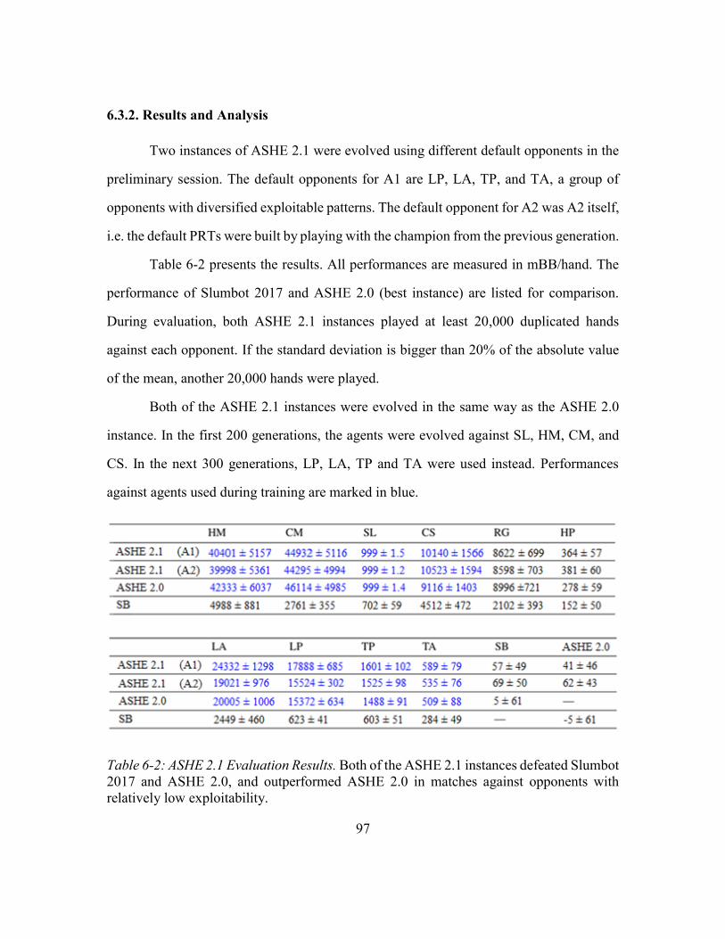
97


Two instances of ASHE 2.1 were evolved using different default opponents in the

preliminary session. The default opponents for A1 are LP, LA, TP, and TA, a group of

opponents with diversified exploitable patterns. The default opponent for A2 was A2 itself,

i.e. the default PRTs were built by playing with the champion from the previous generation.

Table 6-2 presents the results. All performances are measured in mBB/hand. The

performance of Slumbot 2017 and ASHE 2.0 (best instance) are listed for comparison.

During evaluation, both ASHE 2.1 instances played at least 20,000 duplicated hands

against each opponent. If the standard deviation is bigger than 20% of the absolute value

of the mean, another 20,000 hands were played.

Both of the ASHE 2.1 instances were evolved in the same way as the ASHE 2.0

instance. In the first 200 generations, the agents were evolved against SL, HM, CM, and

CS. In the next 300 generations, LP, LA, TP and TA were used instead. Performances

against agents used during training are marked in blue.

Table 6-2: ASHE 2.1 Evaluation Results. Both of the ASHE 2.1 instances defeated Slumbot

2017 and ASHE 2.0, and outperformed ASHE 2.0 in matches against opponents with

relatively low exploitability.

98

The rest of this section summarizes key discoveries and conclusions from these

results. First, both A1 and A2 outperformed ASHE 2.0 when playing against opponents of

relatively low exploitability. In particular, both instances defeated SB with statistically

significant margin. These results indicate that the advanced PRTs in ASHE 2.1 are

particularly effective against strong opponents for their ability to extract complex patterns

in opponent strategies.

Second, both ASHE 2.1 instances exploited RG effectively and defeated ASHE 2.0

in heads-up matches, demonstrating remarkable generalizability to dynamic strategies that

are not seen during training.

Third, both ASHE 2.1 instances are effective against opponents with different level

of exploitability. Thus, the default opponent(s) can be either dynamic (A2) or static (A1).

A group of agents with diversified and highly exploitable patterns and adaptive agents with

relatively low exploitability can both serve the purpose, as long as they allow ASHE to

explore different paths in the default PRTs and develop a good default strategy.

Fourth, agents with advanced PRTs tend to be more effective against opponents

that are similar to their default opponent(s). A1 achieved the highest performance against

LA, LP, TP, and TA, all of which were used as default opponents for the instance. A2

performed best against ASHE 2.0, SB, and HP, whose low-exploitability strategies are

similar to A2 itself. In contrast, when playing against HM or CM, it took longer for the

ASHE 2.1 instances to adapt to these highly exploitable opponents than the ASHE 2.0

instance, resulting in slightly worse performance.

In sum, advanced PRTs allow ASHE to capture board-based patterns in opponent

strategies. The ASHE 2.1 is particularly effective against low-exploitability opponents

defeating both Slumbot 2017 and ASHE 2.0 in heads-up matches.

99

Chapter 7: Recurrent Utility Estimation

In ASHE 2.0, the decision algorithm evaluates the expected utilities for available

actions and selects the action with the highest utility. Hence, utility estimation is critical to

achieving high performance. As is introduced in Subsection 5.1.3, utility estimation in

ASHE 2.0 is based on the assumption that when ASHE bets or raises, the opponent either

folds or calls; if the opponent calls, the game goes to a showdown without more chips

committed to the pot. Clearly, the above assumption may not always hold, especially in

early rounds of betting, i.e. preflop and flop. This assumption simplifies utility estimation,

thus allowing faster decision. However, it can make utility estimation inaccurate, leading

to suboptimal decisions. Thus, this chapter introduces Recurrent Utility Estimation, which

takes possible future moves into consideration and estimates action utilities more

accurately. ASHE 2.2 was built using this technique. Experimental results demonstrate that

the algorithm improves performance against opponents with different level of

exploitability.

7.1. RECURRENT UTILITY ESTIMATION

To evaluate the utilities of available actions more accurately, future moves must be

taken into consideration. For example, slow playing (checking/calling instead of betting or

raising to induce opponent aggression) a big hand is profitable only if the opponent is likely

to bet/raise in the future. Similarly, floating (i.e. calling with a weak hand in order to bluff

later) is a viable option when the opponent is likely to fold under pressure in the next betting

round(s).

Recurrent Utility Estimation relies on advanced PRTs and the LSTM estimators to

predict future moves from the opponent and evaluate showdown values at the terminal

states. Figure 7-1 outlines the algorithm.

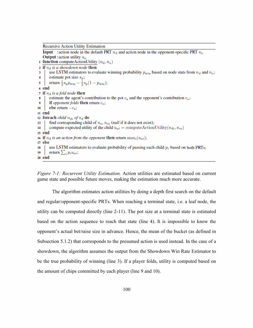
100

Figure 7-1: Recurrent Utility Estimation. Action utilities are estimated based on current

game state and possible future moves, making the estimation much more accurate.

The algorithm estimates action utilities by doing a depth first search on the default

and regular/opponent-specific PRTs. When reaching a terminal state, i.e. a leaf node, the

utility can be computed directly (line 2-11). The pot size at a terminal state is estimated

based on the action sequence to reach that state (line 4). It is impossible to know the

opponent’s actual bet/raise size in advance. Hence, the mean of the bucket (as defined in

Subsection 5.1.2) that corresponds to the presumed action is used instead. In the case of a

showdown, the algorithm assumes the output from the Showdown Win Rate Estimator to

be the true probability of winning (line 3). If a player folds, utility is computed based on

the amount of chips committed by each player (line 9 and 10).

101

Given a node that represents a non-terminal state, the algorithm first computes the

utility for each child node recursively. In other words, the algorithm estimates the utilities

assuming each possible move from the next player to act.

If ASHE is the next player to act, the algorithm assumes that ASHE will select the

action with the highest utility and returns that values (line 16). If the opponent is the next

player to act, a new LSTM module called the Opponent Action Rate Estimator (i.e. OARE,

introduced in Section 7.2), predicts the probability of each opponent action. The utility of

this non-terminal state is the sum of all utilities of the child nodes, weighted by their

corresponding probability (line 18-19).

As the algorithm visits each non-leaf node, the states of the LSTM modules are

saved. Then, inputs derived from the raw game state and the nodes stats in the default and

regular PRT are sent to the SWRE and the OARE. In the rare case where the node stats in

both PRTs are unreliable, utility is estimated using the ASHE 2.0 decision algorithm. The

states of the LSTM modules are restored after the algorithm finishes visiting the node.

When applying Recurrent Utility Estimation in combination with advanced PRTs,

the algorithm may run into board nodes. While community cards in future betting rounds

are not known, the utility can be approximated using the sum of the utilities given each

cluster, weighted by their respective probabilities.

For the first two betting rounds, i.e. preflop and flop, computing the utilities for all

possible paths can be very costly. Therefore, a Monte Carlo method is used to generate

random boards, and the algorithm returns the average utility of all samples. Note that

different boards may fall into the same cluster, and the utility only needs to be computed

once for each cluster/board node. As for the turn, since there is only a single community

card to come, the algorithm traverses all possible paths. Thus, the Recursive Utility

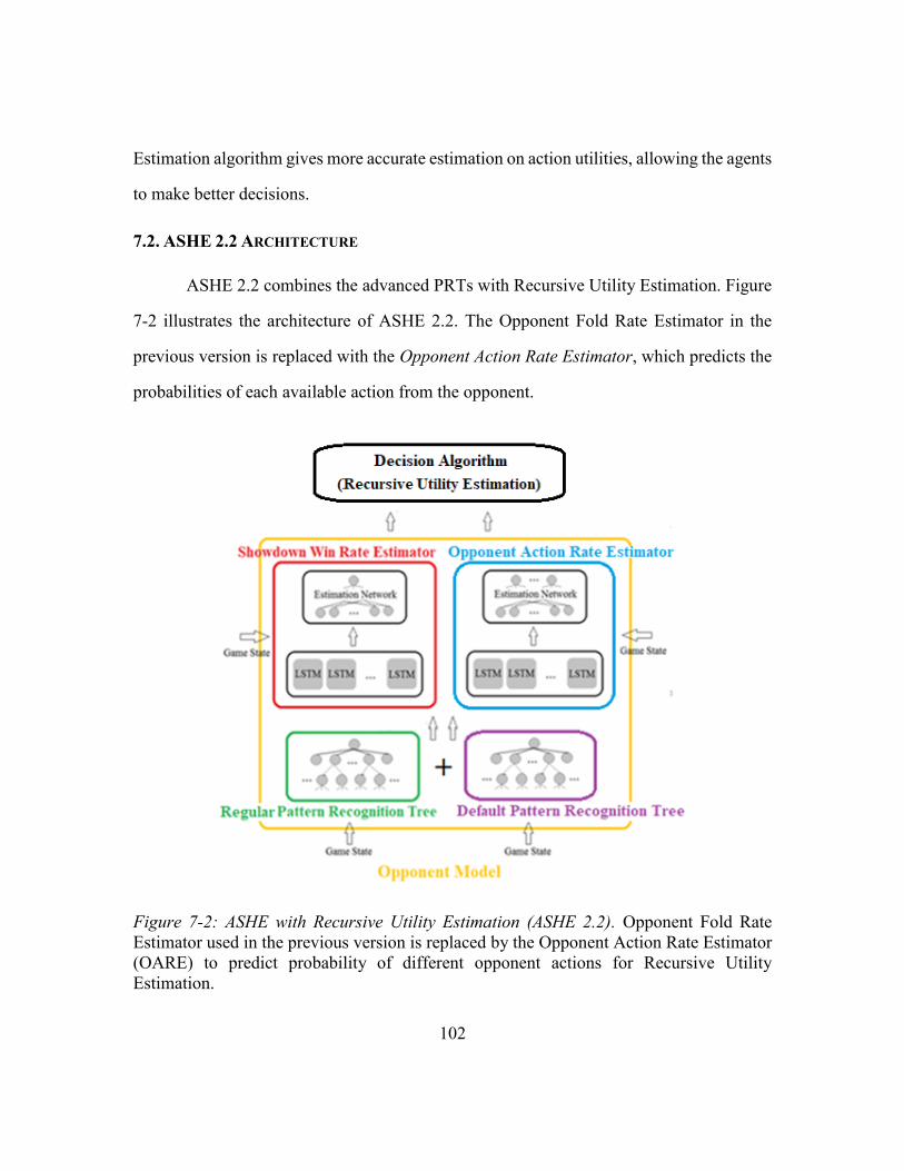
102

Estimation algorithm gives more accurate estimation on action utilities, allowing the agents

to make better decisions.


ASHE 2.2 combines the advanced PRTs with Recursive Utility Estimation. Figure

7-2 illustrates the architecture of ASHE 2.2. The Opponent Fold Rate Estimator in the

previous version is replaced with the Opponent Action Rate Estimator, which predicts the

probabilities of each available action from the opponent.

Figure 7-2: ASHE with Recursive Utility Estimation (ASHE 2.2). Opponent Fold Rate

Estimator used in the previous version is replaced by the Opponent Action Rate Estimator

(OARE) to predict probability of different opponent actions for Recursive Utility

Estimation.

103

Like the OFRE, The OARE consists of a single layer of LSTM blocks and a fully

connected feed-forward estimation network. The output layer of the OARE estimation

network contains nine nodes, corresponding to fold, check/call, and bet/raise in each of the

seven bet-size buckets. These outputs go through a softmax function before being sent to

the decision algorithm. An output is skipped in the softmax if the corresponding action is

not available to the opponent.

To support opponent action prediction other than folding, the PRT node stats are

expanded as follows:

State Frequency (f), showdown counts (csd), and showdown strength (�̅�)

remains the same as defined in Subsection 5.1.2. “Fold counts” in 5.1.2

(cof) is now referred to as the “eventual fold count”, not to be confused

with the new fold counts cf. These node stats are maintained at every

non-leaf node as before.

Fold Counts (cf): the number of times the opponent folding its hand as

the next action.

Check/Call Counts (cc): the number of times the opponent checking or

calling as the next action.

Bet/Raise Counts (1-7, cb1 – cb7): the number of times the opponent

betting or raising in each of the seven buckets as the next action.

The new node stats, i.e. cf, cc, and cb1 to cb7, are maintained only in nodes that

represent a game state where the opponent is the next to act. These nodes correspond to

ASHE’s actions rather than those of the opponent (i.e. ASHE’s decision points).

During runtime, the input features for the SWRE remain the same as specified by

Table 5-1, although the feature “fold rate” is renamed as “eventual fold rate”.

104

The OARE takes all the input features that are sent to the OFRE in the previous

versions, with the exception of the eventual fold rate. In addition, it also takes fold rate,

call/check rate, and bet/raise rates for each bucket as its inputs. These features are defined

as their corresponding count divided by the state frequency (f). In PRT nodes where these

counts are not maintained (i.e. ASHE is the next to act), the features are set to zero. All

features derived from the node stats in the default PRT and regular PRT are linearly

combined as specified in Subsection 6.1.2.

Given a game state, the ASHE 2.2 decision algorithm performs Recursive Utility

Estimation for each available action. In the rare case where the node stats in both PRTs are

unreliable or the action node does not exist, the utility of that action is estimated by the

ASHE 2.0 decision algorithm. The OARE and the SWRE are restored to the current states

(Subsection 5.1.2) after all estimations complete.

Thus, the ASHE 2.2 architecture utilizes the node stats in the advanced PRTs to

predict opponent actions. It is essentially another step towards explicit opponent modeling,

thus allowing decision-making to be more accurate.


This section presents and discusses experimental results on ASHE 2.2, which

integrates advanced PRTs with Recursive Utility Estimation.


Table 7-1 lists key parameter settings for the ASHE 2.2 experiments. Evolution was

extended to 750 generations. Sessions evolving the OARE contained twice as many

generations as those for the SWRE. Monte Carlo sampling size was set to 100 for the first

two betting rounds, which keeps a good balance between fitness and training efficiency.

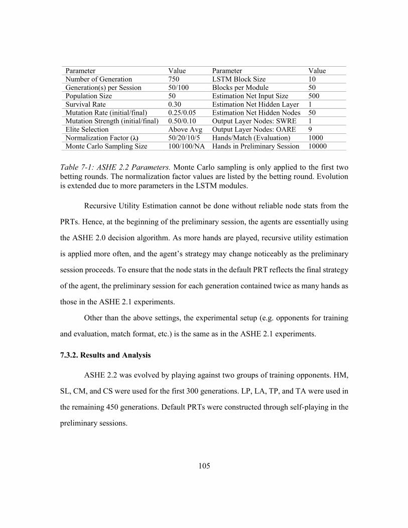
105

Table 7-1: ASHE 2.2 Parameters. Monte Carlo sampling is only applied to the first two

betting rounds. The normalization factor values are listed by the betting round. Evolution

is extended due to more parameters in the LSTM modules.

Recursive Utility Estimation cannot be done without reliable node stats from the

PRTs. Hence, at the beginning of the preliminary session, the agents are essentially using

the ASHE 2.0 decision algorithm. As more hands are played, recursive utility estimation

is applied more often, and the agent’s strategy may change noticeably as the preliminary

session proceeds. To ensure that the node stats in the default PRT reflects the final strategy

of the agent, the preliminary session for each generation contained twice as many hands as

those in the ASHE 2.1 experiments.

Other than the above settings, the experimental setup (e.g. opponents for training

and evaluation, match format, etc.) is the same as in the ASHE 2.1 experiments.


ASHE 2.2 was evolved by playing against two groups of training opponents. HM,

SL, CM, and CS were used for the first 300 generations. LP, LA, TP, and TA were used in

the remaining 450 generations. Default PRTs were constructed through self-playing in the

preliminary sessions.

Parameter Value Parameter Value

Number of Generation 750 LSTM Block Size 10

Generation(s) per Session 50/100 Blocks per Module 50


Survival Rate 0.30 Estimation Net Hidden Layer 1 Mutation Rate (initial/final) 0.25/0.05 Estimation Net Hidden Nodes 50 Mutation Strength (initial/final) 0.50/0.10 Output Layer Nodes: SWRE 1

Elite Selection Above Avg Output Layer Nodes: OARE 9

Normalization Factor (λ) 50/20/10/5 Hands/Match (Evaluation) 1000

Monte Carlo Sampling Size 100/100/NA Hands in Preliminary Session 10000

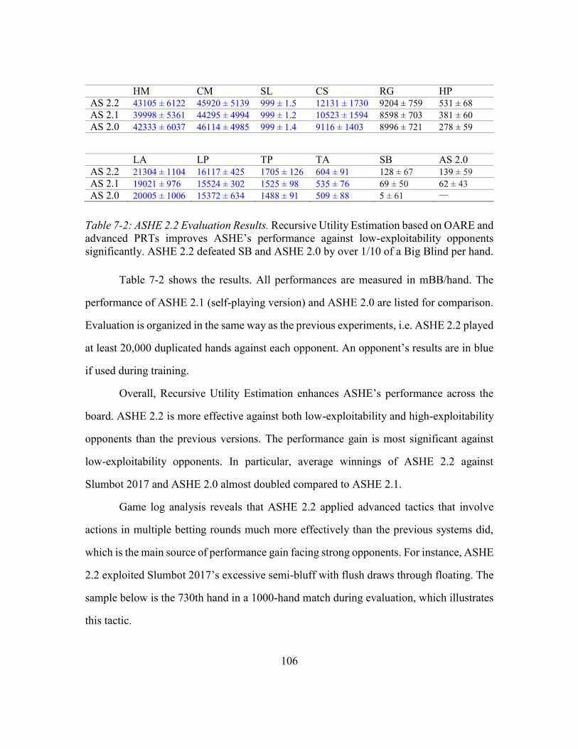
106

HM CM SL CS RG HP AS 2.2 43105 ± 6122 45920 ± 5139 999 ± 1.5 12131 ± 1730 9204 ± 759 531 ± 68

AS 2.1 39998 ± 5361 44295 ± 4994 999 ± 1.2 10523 ± 1594 8598 ± 703 381 ± 60

AS 2.0 42333 ± 6037 46114 ± 4985 999 ± 1.4 9116 ± 1403 8996 ± 721 278 ± 59

LA LP TP TA SB AS 2.0

AS 2.2 21304 ± 1104 16117 ± 425 1705 ± 126 604 ± 91 128 ± 67 139 ± 59

AS 2.1 19021 ± 976 15524 ± 302 1525 ± 98 535 ± 76 69 ± 50 62 ± 43

AS 2.0 20005 ± 1006 15372 ± 634 1488 ± 91 509 ± 88 5 ± 61 —

Table 7-2: ASHE 2.2 Evaluation Results. Recursive Utility Estimation based on OARE and

advanced PRTs improves ASHE’s performance against low-exploitability opponents

significantly. ASHE 2.2 defeated SB and ASHE 2.0 by over 1/10 of a Big Blind per hand.

Table 7-2 shows the results. All performances are measured in mBB/hand. The

performance of ASHE 2.1 (self-playing version) and ASHE 2.0 are listed for comparison.

Evaluation is organized in the same way as the previous experiments, i.e. ASHE 2.2 played

at least 20,000 duplicated hands against each opponent. An opponent’s results are in blue

if used during training.

Overall, Recursive Utility Estimation enhances ASHE’s performance across the

board. ASHE 2.2 is more effective against both low-exploitability and high-exploitability

opponents than the previous versions. The performance gain is most significant against

low-exploitability opponents. In particular, average winnings of ASHE 2.2 against

Slumbot 2017 and ASHE 2.0 almost doubled compared to ASHE 2.1.

Game log analysis reveals that ASHE 2.2 applied advanced tactics that involve

actions in multiple betting rounds much more effectively than the previous systems did,

which is the main source of performance gain facing strong opponents. For instance, ASHE

2.2 exploited Slumbot 2017’s excessive semi-bluff with flush draws through floating. The

sample below is the 730th hand in a 1000-hand match during evaluation, which illustrates

this tactic.

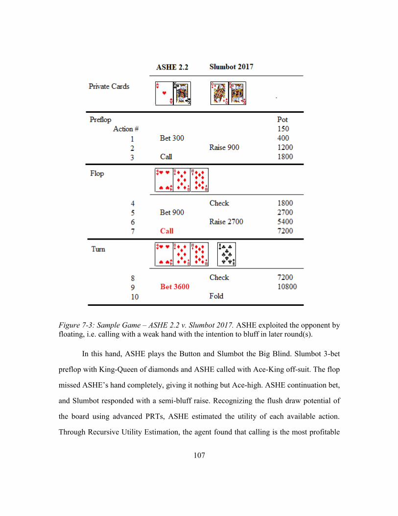
107

Figure 7-3: Sample Game – ASHE 2.2 v. Slumbot 2017. ASHE exploited the opponent by

floating, i.e. calling with a weak hand with the intention to bluff in later round(s).

In this hand, ASHE plays the Button and Slumbot the Big Blind. Slumbot 3-bet

preflop with King-Queen of diamonds and ASHE called with Ace-King off-suit. The flop

missed ASHE’s hand completely, giving it nothing but Ace-high. ASHE continuation bet,

and Slumbot responded with a semi-bluff raise. Recognizing the flush draw potential of

the board using advanced PRTs, ASHE estimated the utility of each available action.

Through Recursive Utility Estimation, the agent found that calling is the most profitable

108

action given the current game state, because the opponent is likely to be holding a flush

draw and fold it to a turn bet if the turn card does not complete the flush. Thus, ASHE

called on the flop, and when the turn card missed the draw, it bluffed with a half-pot bet,

winning the “bluff war” and a big pot.

In contrast, when facing similar situations, ASHE 2.0 tends to fold and ASHE 2.1

tends to re-raise (pot-size/all-in) on the flop. Both options are inferior: folding makes the

opponent’s semi-bluff profitable; re-raising on the flop offers the opponent better odds to

call with two more cards to come and risks much more chips. Note that in order to make

the optimal decision in such situations, future moves and community cards must be taken

into consideration when evaluating action utilities. Hence, Recursive Utility Estimation

and advanced PRTs is necessary for achieving high performance against low-exploitability

opponents.

In sum, ASHE 2.2 outperformed the previous versions consistently and achieved

considerably better results in matches against low-exploitability opponents. Experimental

results show that Recursive Utility Estimation allows the agent to apply advanced poker

tactics more effectively, which is the main source of the performance gain.

109

Chapter 8: Hand Range Analysis

The ASHE 2.0 architecture contains four components: the PRTs, the two LSTM

estimators, i.e. OFRE and SWRE, and the decision algorithm. ASHE 2.1 introduces the

advanced PRTs, ASHE 2.2 replaces OFRE with OARE and employs Recursive Utility

Estimation in the decision algorithm. This chapter focuses on improving SWRE. The idea

is to enhance the accuracy of showdown value estimation by integrating the Hand-Range

Estimation into ASHE 2.2. Experimental results show that such a system is most effective

in modeling and exploiting both high-exploitability and low-exploitability opponents.

8.1. HAND RANGE ANALYSIS

Hand range analysis is one of the most important tools for professional human

players to decide their moves in poker. It means to evaluate the showdown equity of a hand

based on the range of hands the opponent may have.

The probability of the opponent holding certain hand(s) can be inferred from the

action sequence and the community cards. For example, suppose the hero holds AsAc, and

the river board is Kh9h7s|2s|Ah. The hero has top set/three-of-a-kind, a reasonably strong

hand. The villain checks the river, the hero bets half the pot, and the villain raises by the

size of the pot. At this point, the hero is facing a tough decision.

From a hand range analysis perspective, rather than guessing what the villain is

holding at the moment, the hero should ask: what is the range of hands with which the

villain might raise? The hero should take the board, the actions in this hand, and the overall

strategy of the opponent into consideration. Given this board, the villain could be holding

a flush, which crushes hero’s hand. However, flushes may not be the only hands in the

villain’s range. Here, action sequence can provide valuable clues. For instance, suppose

the villain played aggressively preflop, he is likely to have Ace-King, Kings, nines, or even

110

sevens, all of which are worse hands. The opponent’s overall strategy is another important

factor. If the villain is a maniac, it is entirely possible that he is simply bluffing on a “scary

river” with a much worse hand. In contrast, if he plays tight and only raises with strong

hands, the hero’s hand may not be good enough against the villain’s range to justify a call.

Through hand range analysis, good human players estimates showdown value of

their hands more accurately, which usually leads to profitable decisions in the long run.

The Hand Range Estimator in ASEH 2.3 is designed to do the same.

8.2. HAND RANGE ESTIMATOR AND THE ASHE 2.3 ARCHITECTURE

Hand Range Estimator is introduced in ASHE 2.3 to improve showdown equity

evaluation, which is critical for estimating action utility. In Recursive Utility Estimation,

showdown equity, i.e. the probability of winning in a showdown, is used only at terminal

states where all five community cards are dealt out or sampled by Monte Carlo method

(Figure 7-1, line 3-4). In these states, seven out of the 52 cards are ruled out by either the

board or the private cards, leaving the opponent with 990 possible combinations of private

cards. While it is possible to predict opponent hand range based on their type (e.g. one-

pair, two-pair, three-of-a-kind, etc.) like most human players do, it is unnecessary since

what matters is the probability of the opponent holding each of these combinations.

An important trade-off in the design of the Hand Range Estimator is between the

specificity of hands and the complexity of the model. Predicting the probability of each

combination may lead to more accurate estimation of showdown equity. Nevertheless, it

requires a big network, resulting in slow training.

In ASHE 2.3, the HRE estimates the probabilities of the opponent’s hand falling

into one of the nine buckets. These buckets are not defined by the type of hands (e.g. a

flush, straight, etc.). Instead, they correspond to different intervals in the ranking among

111

the 990 possible hands. These intervals are: 1 – 25, 26 – 50, 51 – 100, 101 – 150, 151 –

250, 251 – 350, 351 – 500, 501 – 650, and 651 – 990. The intervals are defined narrower

for higher ranks because high-ranking hands end up in a showdown more often and need

to be distinguished from each other.

To estimate showdown equity using HRE predictions, ASHE’s hand is compared

with the possible hands in the opponent’s range. Suppose a rA is the number of hands that

are stronger than ASHE’s hand, showdown equity pwin is computed as:

𝑝win = 1 − ∑ 𝑝𝑖𝛿(𝑟A, 𝑎𝑖, 𝑏𝑖)

𝑁

𝑖=1

𝛿(𝑟A, 𝑎, 𝑏) = {

0 𝑖𝑓 𝑟A ≤ 𝑎𝑟A − 𝑎

𝑏 − 𝑎 𝑖𝑓 𝑎 < 𝑟A ≤ 𝑏

1 𝑖𝑓 𝑏 < 𝑟A

where N is the number of intervals (N = 9), ai and bi are the boundaries of interval i, and pi

is the HRE prediction for interval i.

Similar to the OARE in ASHE 2.2, the HRE consists of a single layer of LSTM

blocks and a fully-connected feed-forward estimation network with one hidden layer and

nine output nodes. Softmax function is applied to normalize the outputs. Input features for

the HRE are the same as those for the SWRE. As the Recursive Utility Estimation

algorithm visits a node, the states of the HRE are saved. The inputs are then sent to the

HRE. The LSTM states are restored before the algorithm returns from the PRT node.

Figure 8-1 presents the architecture of ASHE 2.3. Note that SWRE is replaced by

the HRE to provide showdown equity estimation based on hand range. The ASHE 2.3

architecture is the most advanced version of the system in this dissertation and integrates

all upgraded components introduced in the previous chapters.

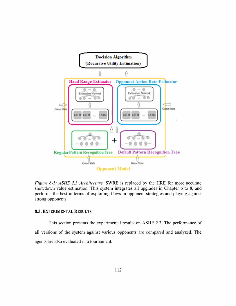
112

Figure 8-1: ASHE 2.3 Architecture. SWRE is replaced by the HRE for more accurate

showdown value estimation. This system integrates all upgrades in Chapter 6 to 8, and

performs the best in terms of exploiting flaws in opponent strategies and playing against

strong opponents.


This section presents the experimental results on ASHE 2.3. The performance of

all versions of the system against various opponents are compared and analyzed. The

agents are also evaluated in a tournament.

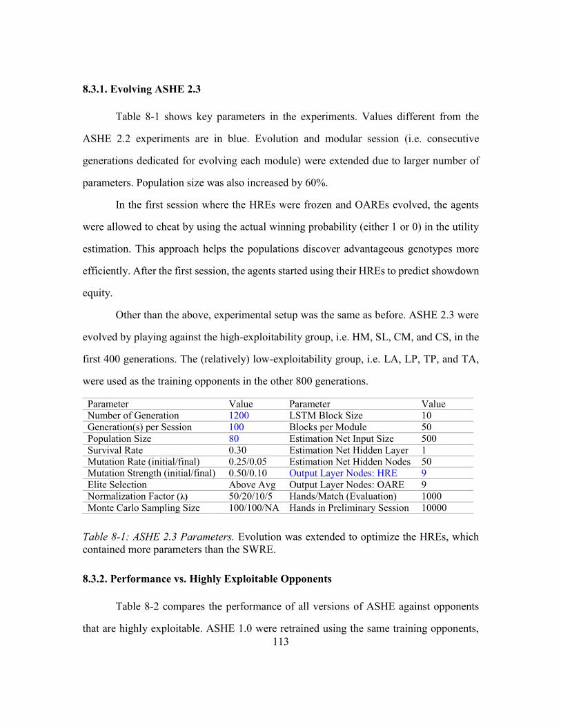
113

8.3.1. Evolving ASHE 2.3

Table 8-1 shows key parameters in the experiments. Values different from the

ASHE 2.2 experiments are in blue. Evolution and modular session (i.e. consecutive

generations dedicated for evolving each module) were extended due to larger number of

parameters. Population size was also increased by 60%.

In the first session where the HREs were frozen and OAREs evolved, the agents

were allowed to cheat by using the actual winning probability (either 1 or 0) in the utility

estimation. This approach helps the populations discover advantageous genotypes more

efficiently. After the first session, the agents started using their HREs to predict showdown

equity.

Other than the above, experimental setup was the same as before. ASHE 2.3 were

evolved by playing against the high-exploitability group, i.e. HM, SL, CM, and CS, in the

first 400 generations. The (relatively) low-exploitability group, i.e. LA, LP, TP, and TA,

were used as the training opponents in the other 800 generations.

Table 8-1: ASHE 2.3 Parameters. Evolution was extended to optimize the HREs, which

contained more parameters than the SWRE.

8.3.2. Performance vs. Highly Exploitable Opponents

Table 8-2 compares the performance of all versions of ASHE against opponents

that are highly exploitable. ASHE 1.0 were retrained using the same training opponents,

Parameter Value Parameter Value Number of Generation 1200 LSTM Block Size 10

Generation(s) per Session 100 Blocks per Module 50


Survival Rate 0.30 Estimation Net Hidden Layer 1 Mutation Rate (initial/final) 0.25/0.05 Estimation Net Hidden Nodes 50 Mutation Strength (initial/final) 0.50/0.10 Output Layer Nodes: HRE 9

Elite Selection Above Avg Output Layer Nodes: OARE 9

Normalization Factor (λ) 50/20/10/5 Hands/Match (Evaluation) 1000

Monte Carlo Sampling Size 100/100/NA Hands in Preliminary Session 10000

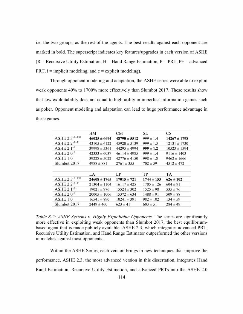
114

i.e. the two groups, as the rest of the agents. The best results against each opponent are

marked in bold. The superscript indicates key features/upgrades in each version of ASHE

(R = Recursive Utility Estimation, H = Hand Range Estimation, P = PRT, P+ = advanced

PRT, i = implicit modeling, and e = explicit modeling).

Through opponent modeling and adaptation, the ASHE series were able to exploit

weak opponents 40% to 1700% more effectively than Slumbot 2017. These results show

that low exploitability does not equal to high utility in imperfect information games such

as poker. Opponent modeling and adaptation can lead to huge performance advantage in

these games.

HM CM SL CS ASHE 2.3eP+RH 46025 ± 6694 48790 ± 5512 999 ± 1.4 14267 ± 1798

ASHE 2.2eP+R 43105 ± 6122 45920 ± 5139 999 ± 1.5 12131 ± 1730

ASHE 2.1eP+ 39998 ± 5361 44295 ± 4994 999 ± 1.2 10523 ± 1594

ASHE 2.0eP 42333 ± 6037 46114 ± 4985 999 ± 1.4 9116 ± 1403

ASHE 1.0i 39228 ± 5022 42776 ± 4150 998 ± 1.8 9462 ± 1666

Slumbot 2017 4988 ± 881 2761 ± 355 702 ± 59 4512 ± 472

LA LP TP TA

ASHE 2.3eP+RH 24608 ± 1765 17015 ± 721 1744 ± 153 626 ± 102

ASHE 2.2eP+R 21304 ± 1104 16117 ± 425 1705 ± 126 604 ± 91

ASHE 2.1eP+ 19021 ± 976 15524 ± 302 1525 ± 98 535 ± 76

ASHE 2.0eP 20005 ± 1006 15372 ± 634 1488 ± 91 509 ± 88

ASHE 1.0i 16541 ± 890 10241 ± 391 982 ± 102 134 ± 59

Slumbot 2017 2449 ± 460 623 ± 41 603 ± 51 284 ± 49

Table 8-2: ASHE Systems v. Highly Exploitable Opponents. The series are significantly

more effective in exploiting weak opponents than Slumbot 2017, the best equilibrium-

based agent that is made publicly available. ASHE 2.3, which integrates advanced PRT,

Recursive Utility Estimation, and Hand Range Estimator outperformed the other versions

in matches against most opponents.

Within the ASHE Series, each version brings in new techniques that improve the

performance. ASHE 2.3, the most advanced version in this dissertation, integrates Hand

Rand Estimation, Recursive Utility Estimation, and advanced PRTs into the ASHE 2.0

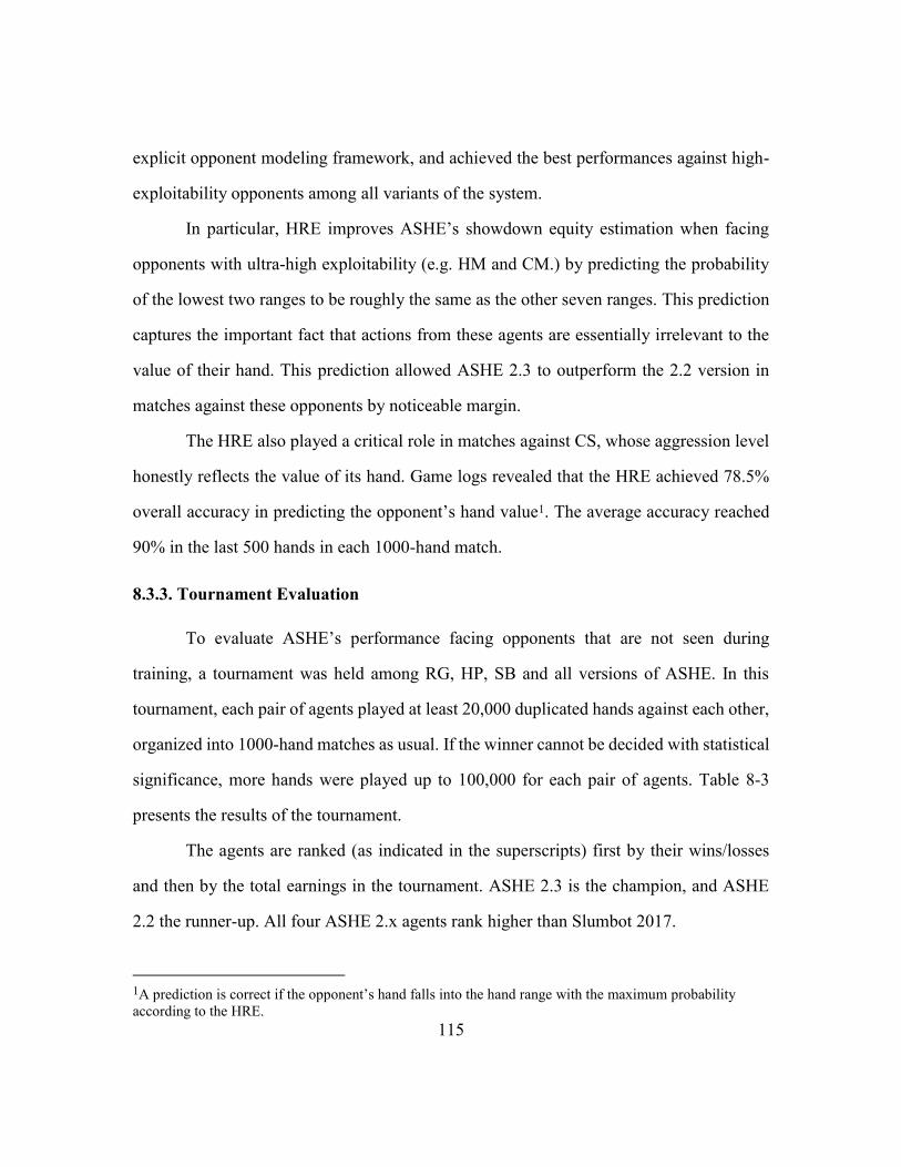
115

explicit opponent modeling framework, and achieved the best performances against high-

exploitability opponents among all variants of the system.

In particular, HRE improves ASHE’s showdown equity estimation when facing

opponents with ultra-high exploitability (e.g. HM and CM.) by predicting the probability

of the lowest two ranges to be roughly the same as the other seven ranges. This prediction

captures the important fact that actions from these agents are essentially irrelevant to the

value of their hand. This prediction allowed ASHE 2.3 to outperform the 2.2 version in

matches against these opponents by noticeable margin.

The HRE also played a critical role in matches against CS, whose aggression level

honestly reflects the value of its hand. Game logs revealed that the HRE achieved 78.5%

overall accuracy in predicting the opponent’s hand value1. The average accuracy reached

90% in the last 500 hands in each 1000-hand match.

8.3.3. Tournament Evaluation

To evaluate ASHE’s performance facing opponents that are not seen during

training, a tournament was held among RG, HP, SB and all versions of ASHE. In this

tournament, each pair of agents played at least 20,000 duplicated hands against each other,

organized into 1000-hand matches as usual. If the winner cannot be decided with statistical

significance, more hands were played up to 100,000 for each pair of agents. Table 8-3

presents the results of the tournament.

The agents are ranked (as indicated in the superscripts) first by their wins/losses

and then by the total earnings in the tournament. ASHE 2.3 is the champion, and ASHE

2.2 the runner-up. All four ASHE 2.x agents rank higher than Slumbot 2017.

1A prediction is correct if the opponent’s hand falls into the hand range with the maximum probability

according to the HRE.

116

Table 8-3: Tournament Evaluation Results. The colors red, yellow, and green indicate the

agent in the row losing to, tying with, or winning the agent in the column. The ASHE

Systems are effective against both static and dynamic opponents that are not seen during

evolution. ASHE 2.1 and later versions of the system defeated Slumbot 2017. ASHE 2.3

and ASHE 2.2 performed the best in matches against low-exploitability opponents.

ASHE 2.3 and 2.2 were both undefeated in the tournament. The two agents tied

statistically after 1000 matches (100,000 duplicated hands) against each other. The HRE

gave ASHE 2.3 an edge in total earnings by beating RG with a bigger margin. Therefore,

the championship was awarded to ASHE 2.3.

Empirical results indicate that the HRE is more effective in predicting showdown

values against weaker opponents. The performance advantage of ASHE 2.3 over ASHE

2.2 tends to be smaller when facing low-exploitability opponents. In heads-up matches

between these two agents, overall the accuracy of the HRE predictions was 32.7%, which

increased to around 35% in the last 500 hands. Note that the accuracy was significantly

lower than the accuracy when facing CS. This difference is likely to be caused by

adaptation, which makes hand range prediction more difficult.

Overall, ASHE 2.3 and 2.2 demonstrate strong generalizability to opponents that

are not seen during training. In particular, both agents exploited ASHE 1.0 effectively by

check-raising and/or slow playing their strong hands. They were also able to discover and

exploit a big “leak” in HP’s strategy: the agent’s calling range was too tight when facing

AS 2.3 AS 2.2 AS 2.1 AS 2.0 SB HP AS 1.0 RG

AS 2.31st 9.5 109 132 141 549 1094 11227

AS 2.22nd -9.5 98 139 128 531 1150 9204

AS 2.13rd -109 -98 62 69 381 638 8598

AS 2.04th -132 -139 -62 11.4 278 581 8996

SB5th -141 -128 -69 -11.4 152 269 2102

HP7th -549 -531 -381 -278 -152 89 1413

AS 1.06th -1094 -1150 -638 -581 -269 -89 7984

RG8th -11227 -9204 -8598 -8996 -2102 -1413 -7984

117

raises on the river. Furthermore, the performance of ASHE 2.3 and 2.2 in matches against

SB, HP, RG and the previous versions in the ASHE Series show that the system can model

and exploit both dynamic and static strategies effectively.

Thus, the ASHE Series provide a new approach to building adaptive agents for

HUNL and other imperfect information games. The next chapter summarizes this line of

research and discusses potential directions for future work.

118

Chapter 9: Discussion and Future Work

This chapter discusses ASHE’s limitations and suggests potential directions for

future work in two aspects: (1) training and evaluation, (2) reinforcement learning, and (3)

end-to-end learning and generalization to other problem domains.

9.1. TRAINING AND EVALUATION

The ASHE agents are mainly evolved by playing against opponents that are highly

or moderately exploitable. Empirical results demonstrate the remarkable generalizability

of this approach. A set of reasonably diversified training opponents is usually sufficient for

evolving agents that can generalize well to new opponents with much lower exploitability.

Nevertheless, experimental results also indicate that training opponents with lower

exploitability tend to yield better performance than highly exploitable opponents with the

same types of weakness.

In addition, opponents can be organized into training groups according to their level

of exploitability. During evolution, training groups with higher exploitability can be used

first, followed by groups with lower exploitability. This method promotes adaptation and

exploitation more effectively, which leads to higher performance. Hence, it would be

interesting to see how performance can be improved if more low-exploitability agents are

used during training and evaluation.

While the plan is straightforward, it can be difficult to access high-quality HUNL

agents. Most state-of-the-art poker agents such as DeepStack and Libratus are not publicly

available due to the huge computational resource requirement. The Annual Computer

Poker Competition (ACPC) used to be the best way to access high-quality agents.

Submissions were made accessible to participants by convention. A prototype of ASHE

2.0 was submitted to the 2017 ACPC and ranked the seventh among fifteen submissions in

119

overall performance (http://www.computerpokercompetition.org). However, due to budget

issues and technical difficulties, the 2017 results were incomplete, and the submissions

were not made available. In addition, the 2018 ACPC results are not released at the time

of writing, and the submissions are also not accessible.

For the above reason, the best available low-exploitability opponent, i.e. Slumbot,

was used in the experiments in this dissertation. Slumbot 2016 (used in Chapter 4) was the

runner-up of for the 2016 ACPC, and Slumbot 2017 (used in Chapter 5 to 8) is the latest

version of the agent. A potential direction for future work is to evolve and evaluate the

system with stronger opponents when they become available.

9.2. REINFORCEMENT LEARNING

Neuroevolution has been shown to be more effective than standard reinforcement

learning techniques in many benchmark tasks with sparse reinforcement such as helicopter

control [Koppejan and Whiteson, 2009] and pole balancing [Moriarty and Miikkulainen

1996; Heidrich-Meisner and Igel, 2009]. In particular, compact and effective neural

network structures can be discovered efficiently through genetic algorithms such as NEAT

[Stanley and Miikkulainen, 2002]. Thus, this dissertation employs evolutionary methods

for training the RNN-based opponent models in ASHE.

However, it is also possible to apply reinforcement learning techniques to building

computer agents for poker and other imperfect information games. Heinrich and Silver

[2016] combined fictitious self-play with deep reinforcement learning to approximate Nash

equilibrium strategies in Leduc poker and Limit Holdem, whose performance approached

the state of the art. Nevertheless, the agents were not adaptive. Hence, a possible direction

for future work is to apply deep RL to opponent modeling and exploitation in HUNL. For

120

instance, earnings/losses in each hand can be used as rewards to adjust the agent’s actions

during lifetime, thus allowing the agents to adapt to different opponent strategies.

9.3. GENERALIZATION

In principle, the architectural framework of the ASHE Series and the evolutionary

method to train the system are applicable to other domains with imperfect information, if

they are modeled as a formal game. Thus, another direction for future work is to generalize

the proposed method in other problem domains.

A natural extension of the system is to develop an agent for multi-player tournament

poker. The main challenge is to represent the enormous game state space efficiently. One

possible approach is to train additional neural network modules to identify the “strongest

opponent”, thus converting the multi-player game into a heads-up game. Another option is

to train a neural network encoder to compress the game states. Agents can be trained to

operate on the compressed/abstracted game instead, which is similar to abstraction in Nash

equilibrium approximation.

In addition, ASHE can be applied to games other than poker. For instance, in a

security game between the attacker and the defender, PRTs can be constructed to represent

the action sequences. LSTM modules can be evolved to predict the form and target of the

attacks. Recursive Utility Estimation can be used to estimate expected utility for each

defensive measure. However, as in the case of poker, feature engineering is necessary in

adjusting the system. In particular, the PRT node stats and the input features for the LSTM

modules are defined based on domain knowledge, which is problem-specific.

While most existing methods in building computer agents for imperfect information

games (e.g. CFR and other equilibrium approximation techniques) rely heavily on domain

knowledge, such reliance makes generalization more difficult. Therefore, another potential

121

direction for future work is to improve generalizability by reducing the dependency of

domain-specific knowledge and human interference in feature extraction. The goal is to

develop an end-to-end RNN-based adaptive poker agents with high performance.

Yakovenko, et al [2016] proposed creating a poker playing system using a unified poker

representation. A convolutional-neural-network-based model was developed to learn the

patterns in three variants of poker, including Limit Texas Holdem. This approach may be

combined with the ASHE 2.x architecture to reduce expert knowledge needed in feature

extraction.

122

Chapter 10: Contributions and Conclusion

This chapter summarizes the work from Chapter 4 to 8. Section 10.1 outlines the

contributions of this work. Section 10.2 evaluates its impact.

10.1. CONTRIBUTIONS

From ASHE 1.0 to ASHE 2.3, the ASHE Series provide an effective new approach

to building high-performance adaptive agents for HUNL and other imperfect information

games. ASHE 1.0 uses LSTM modules, i.e. the opponent module and the game module, to

extract and encode opponent strategy and game states from the current hand. These features

are then sent to a feed-forward neural network, i.e. the decision network, which calculates

an aggression score. Actions are chosen by a rule-based decision algorithm according to

the score. To address the problem of insufficient training data for supervised learning, the

system is evolved through neuroevolution. Tiered Survival and Elite Reproduction (TSER)

is introduced to resolve the dilemma between offspring quality and genotype preservation

in a stochastic game. Fitness is evaluated by Average Normalized Earnings (ANEs) against

highly exploitable opponents that require different counterstrategies for exploitation.

Empirical results show that ASHE 1.0 is far more effective than Slumbot 2016, one

of the top-ranking Nash-equilibrium-based agents, in matches against highly exploitable

opponents. This result demonstrates ASHE’s ability to model and exploit the opponents.

In addition, ASHE 1.0 evolved through playing against highly exploitable opponents can

generalize to stronger opponents that are not seen in training. However, the agent is

defeated by Slumbot in heads-up matches with relatively big margins.

ASHE 1.0 validates the design principle of RNN-based adaptive agents in large-

scale imperfect information games and lays a solid foundation for discovering opponent

models through evolutionary methods. The main shortcoming is that opponent modeling

123

in ASHE 1.0 is implicit. The agent does not predict opponent actions or evaluate showdown

value. Everything is encoded by the aggression score, which leads to less accurate decision-

making.

ASHE 2.0 solves this problem with an extended architecture that models the

opponents explicitly. LSTM neural networks are employed to estimate the showdown

value and predict the opponent’s probability of folding given bets/raises of different size.

The decision algorithm evaluates the expected utilities of available actions using these

predictions and decides the agent’s move accordingly. A new data structure, i.e. Pattern

Recognition Tree (PRT), is introduced to maintain statistics on opponent strategy given

different game states. The PRTs benefit the system in two ways: (1) they provide useful

features for the LSTM estimators, and (2) they reduce the size of the LSTM modules, thus

improving training efficiency.

Experimental results show that ASHE 2.0 inherits the ability to model and exploit

weak opponents from ASHE 1.0. In addition, the agent ties statistically with Slumbot 2017,

which is an upgrade and much stronger version of the equilibrium-based agent used in the

ASHE 1.0 experiments. Moreover, the agent can model and exploit both static and dynamic

opponents effectively. ASHE 2.0 establishes an architectural framework for LSTM-based

adaptive agents with explicit opponent modeling. Key components in the architectural

framework, i.e. the PRTs, the LSTM estimators, and the decision algorithm are then

upgraded in ASHE 2.1 to 2.3, each focusing on a different aspect.

ASHE 2.1 introduces the advanced PRTs, which contain default PRTs and board-

texture-based PRTs. The former allows the agent to make better decisions facing new

opponents or infrequent game states, and the latter enables the agent to extract subtle

patterns in opponent strategy that are based on the texture of the board. The advanced PRTs

124

are particularly effective against low-exploitability opponents; ASHE 2.1 defeats both

ASHE 2.0 and Slumbot 2017 by statistically significant margins.

ASHE 2.2 introduces Recursive Utility Estimation to evaluate action utility more

accurately. This technique allows the agent to take future moves into consideration when

choosing its actions. The LSTM estimators are extended to predict probability of different

actions from the opponent. Experimental results show that Recursive Utility Estimation

allows ASHE to apply advanced poker tactics more effectively, thus enhancing

performance against both high and low exploitability opponents.

ASHE 2.3 introduces Hand Range Estimator (HRE) to improve showdown value

estimation. The HRE predicts the probability of the opponent’s hand falling into different

hand strength interval. Showdown values are then calculated based on statistical rules.

Empirical results indicate that the HRE enhances overall performance of the agent and is

especially effective in predicting the hand range of high-exploitability opponents.

Tournament evaluation show that ASHE 2.3 has the best overall performance among the

ASHE series, tying heads-up against ASHE 2.2 and defeating all other versions as well as

Slumbot 2017.

Thus, the ASHE series of poker agents provide an effective new approach to

building RNN-based adaptive agents for HUNL through evolutionary method. The

architectural framework and genetic algorithm should be generalizable to other imperfect

information games.

10.2. CONCLUSION

This dissertation presents the first evolutionary method for building RNN-based

adaptive agents that model and exploit their opponents in Heads-Up No-Limit Holdem. A

series of poker agents called Adaptive System for Holdem (ASHE) were built to evaluate

125

the proposed approach. Experimental results show that compared to Nash-equilibrium-

based agents, the ASHE Series are generally far more effective against flawed strategies

due to opponent modeling and adaptation. Moreover, given reasonably diversified training

opponents, ASHE 2.x are able to model and exploit both static and dynamic opponent

strategies with much lower exploitability. In particular, ASHE 2.1 and later versions of the

system were able to defeat top-ranking equilibrium-based agents in heads-up matches.

Thus, this dissertation provides an effective new approach for building adaptive

agents for poker and other imperfect information games and points out a promising new

direction for research on such games. In particular, opponent modeling and exploitation

using evolved recurrent neural networks may be the next step beyond Nash equilibrium

approximation for building computer agents for imperfect information games. In the future,

the ASHE architecture and evolutionary method in the dissertation can applied to other

decision-making problems with imperfect information.

126

References

Bard, N., Johanson, M., Burch, N., and Bowling, M. (2013). Online Implicit Agent

Modeling. In Proceedings of the 12th International Conference on Autonomous

Agents and Multi-agent Systems (AAMAS 2013), Saint Paul, Minnesota, USA.

Billings, D., Papps, D., Schaeffer, J., and Szafron, D. (1998). Opponent Modeling in Poker.

In Proceedings of the Joint Conference of AAAI/IAAI, 1998.

Billings, D., Davidson, A., Schaeffer. J, and Szafron, D. (2002). The challenge of poker.

Artificial Intelligence 134, 201–240.

Billings, D., Burch, N., Davidson, A., Holte, R., Schaeffer, J., Schauenberg, T., Szafron,

D. (2003). Approximating Game-Theoretic Optimal Strategies for Full-scale Poker.

In The Eighteenth International Joint Conference on Artificial Intelligence.

Billings, D. (2006). Algorithms and Assessment in Computer Poker. Ph.D. Dissertation,

University of Alberta.

Bowling, M., Burch, N., Johanson, M., and Tammelin, O. (2015). Heads-up limit holdem

poker is solved. Science, 347(6218):145–149.

Brown, N., and Sandholm, T. (2014). Regret transfer and parameter optimization. In

Proceedings of the AAAI Conference on Artificial Intelligence (AAAI).

Brown, N. and Sandholm, T. (2017). Safe and Nested Endgame Solving for Imperfect-

Information Games. In the AAAI workshop on Computer Poker and Imperfect

Information Games.

Brown, N., Ganzfried, S., and Sand-holm, T. (2015). Hierarchical Abstraction, Distributed

Equilibrium Computation, and Post-Processing, with Application to a Champion

No-Limit Texas Hold’em Agent. In Proceedings of the International Conference

on Autonomous Agents and Multi-agent Systems.

Burch, N., Johanson, M., and Bowling, M. (2014). Solving Imperfect Information Games

Using Decomposition. In AAAI Conference on Artificial Intelligence (AAAI).

Cai, G., Wurman, P. (2005). Monte Carlo Approximation in Incomplete Information,

Sequential Auction Games, Decision Support Systems, v.39 n.2, p.153-168.

Davidson, A., Billings, D., Schaeffer, J., and Szafron, D. (2000). Improved Opponent

Modeling in Poker. In International Conference on Artificial Intelligence, ICAI’00.

Doetsch, P., Kozielski, M., and Ney, H. (2014). Fast and Robust Training of Recurrent

Neural Networks for Offline Handwriting Recognition. In the 14th International

Conference on Frontiers in Handwriting Recognition.

127

Ekmekci, O., and Sirin, V. (2013). Learning Strategies for Opponent Modeling in Poker.

In Proceedings of Workshops at the Twenty-Seventh AAAI Conference on Artificial

Intelligence. Bellevue: AAAI Press (pp. 6-12).

Fan, Y., Qian, Y., Xie, F., and Soong, F. (2014). TTS Synthesis with Bidirectional LSTM-

based Recurrent neural networks. In Proc. Interspeech.

Fitzgerald, A. (2015). Range Analysis: The Correct Way to Analyze Poker Hands. In

Jonathan Little’s Excelling at No-Limit Hold’em, D&B Publishing.

Ganzfried, S. (2016). Bayesian Opponent Exploitation in Imperfect-Information Games.

In AAAI Workshop on Computer Poker and Incomplete Information.

Ganzfried, S. and Sandholm, T. (2011). Game Theory-Based Opponent Modeling in Large

Imperfect-Information Games. In Proceedings of the International Conference on

Autonomous Agents and Multi-Agent Systems.

Ganzfried, S. and Sandholm, T. (2014). Potential-aware Imperfect-Recall Abstraction with

Earth-Mover’s Distance in Imperfect Information Games. In AAAI Workshop on

Computer Poker and Imperfect Information Games.

Ganzfried, S. and Sandholm, T. (2015a). Endgame Solving in Large Imperfect Information

Games. In International Conference on Autonomous Agents and Multi-Agent

Systems (AAMAS).

Ganzfried, S. and Sandholm, T. (2015b). Safe Opponent Exploitation. In ACM

Transactions on Economics and Computation, 3(2), 8.

Gilpin, A.; Hoda, S.; Pena, J.; and Sandholm, T. (2007a). Gradient-based Algorithms for

Finding Nash Equilibria in Extensive Form Games. In International Workshop on

Internet and Network Economics (WINE).

Gilpin, A., Sandholm, T., and Sorensen, T. (2007b). Potential-aware Automated

Abstraction of Sequential Games. In Proceedings of the 22nd national conference

on Artificial intelligence, pp.50-57, Vancouver, British Columbia, Canada.

Gilpin, A. and Sandholm, T. (2005). Optimal Rhode Island Hold’em poker, in Proceedings

of the 20th national conference on Artificial intelligence, p.1684-1685, Pittsburgh,

Pennsylvania.

Gilpin, A. and Sandholm, T. (2006a). A Competitive Texas Holdem Poker Player via

Automated Abstraction and Real-time Equilibrium Computation. In Proceedings

of the National Conf. on Artificial Intelligence (AAAI).

Gilpin, A., and Sandholm, T. (2006b). Finding Equilibria in Large Extensive Form Games

of Imperfect Information. In Proceedings of the 7th ACM conference on Electronic

commerce.

128

Gilpin, A. and Sandholm, T. (2008a). Solving Two-Person Zero-Sum Repeated Games of

Incomplete Information. In Proceedings of the Seventh International Conference

on Autonomous Agents and Multi-Agent Systems.

Gilpin, A., and Sandholm, T. (2008b). Expectation-based Versus Potential-aware

Automated Abstraction in Imperfect Information Games: An Experimental

Comparison Using Poker. In Proceedings of theAAAI Conference on Artificial

Intelligence (AAAI).

Gomez, F. and Miikkulainen, R (1999). Solving Non-markovian Control Tasks with

Neuroevolution. In Proceedings of the Sixteenth International Joint Conference on

Artificial Intelligence, pp. 1356–1361, San Francisco, California, USA.

Graves, A., and Schmidhuber, J. (2005). Framewise Phoneme Classification with

Bidirectional LSTM and Other Neural Network Architectures. Neural Networks,

18(5–6):602–610.

Graves, A., Liwicki, M., Bunke, H., Schmidhuber, J., and Fernandez, S. (2008).

Unconstrained Online Handwriting Recognition with Recurrent Neural Networks.

In Advances in Neural Information Processing Systems, pp. 577–584.

Greff, K., Srivastava, R. K., Jan, K., Steunebrink, B. R., and Schmidhuber, J. (2015).

LSTM: a Search Space Odyssey. arXiv preprint arXiv:1503.04069.

Gruau, F., Whitley, D., and Pyeatt, L. (1996). A Comparison between Cellular Encoding

and Direct Encoding for Genetic Neural Networks. In Proceedings of the First

Annual Conference, pp. 81–89, MIT Press, Cambridge, Massachusetts.

Heidrich-Meisner, V. and Igel, C. (2009). Neuroevolution Strategies for Episodic

Reinforcement Learning, Journal of Algorithms, Vol 64, pp 152-168.

Heinrich, J. and Silver, D. (2016). Deep Reinforcement Learning from Self-play in

Imperfect Information Games. In NIPS 2016 Deep Reinforcement Learning

Workshop.

Hochreiter, S. and Schmidhuber, J. (1997). Long Short Term Memory. Neural

Computation 9, pp 1735–1780.

Hoda, S., Gilpin, A., and Pena, J. (2006). A Gradient-based Approach for Computing Nash

Equilibria of Large Sequential Games. In INFORMS.

Jackson, E. (2016). Compact CFR. In AAAI Work-shop on Computer Poker and Imperfect

Information Games, Phoenix, AZ, USA.

Jackson, E. (2017). Targeted CFR. In AAAI Work-shop on Computer Poker and Imperfect

Information Games, San Francisco, CA, USA.

Johanson, M. and Bowling, M. (2009). Data Biased Robust Counter Strategies, In

Proceedings of the Twelfth International Conference on Artificial Intelligence and

Statistics (AISTATS).

129

Johanson, M. (2013). Measuring the Size of Large No-Limit Poker Games.

arXiv:1302.7008 [cs.GT].

Johanson, M., Burch, N., Valenzano, R., and Bowling, M. (2013). Evaluating State-space

Abstractions in Extensive Form Games. In Proceedings of the International

Conference on Autonomous Agents and Multi-Agent Systems (AAMAS).

Johanson, M., Zinkevich, M., and Bowling, M. (2008). Computing Robust Counter-

Strategies. In Advances in Neural Information Processing Systems 20 (NIPS).

Koller, D., Megiddo, N., and von Stengel, B. (1996). Efficient Computation of Equilibria

for Extensive Two-person Games. In Games and Economic Behavior 14(2):247–

259.

Koller, D. and Pfeffer, A. (1997). Representations and Solutions for Game-theoretic

Problems. In Artificial Intelligence, pages 167–215.

Koppejan, R. and Whiteson, S. (2009) Neuroevolutionary Reinforcement Learning for

Generalized Helicopter Control, In Proceedings of the 11th Annual Conference on

Genetic and Evolutionary Computation (GECCO 09), pp 145-152.

Korb, K., Nicholson, A., and Jitnah, N. (1999). Bayesian Poker. In Proceedings of the

Fifteenth Conference on Uncertainty in Artificial Intelligence, pp. 343-350.

Morgan Kaufmann Publishers Inc.

Koutnik, J., Schmidhuber, J., and Gomez, F. (2014). Evolving Deep Unsupervised

Convolutional Networks for Vision-based Reinforcement Learning. In Proceedings

of the 2014 Conference on Genetic and Evolutionary Computation (GECCO 2014),

pp. 541–548.

Kuhn, H. (1950). A Simplified Two-person Poker. Contributions to the Theory of Games,

1:97–103.

Lanctot, M., Waugh, K., Zinkevich, M., and Bowling, M. (2009). Monte Carlo Sampling

for Regret Minimization in Extensive Games. In Advances in Neural Information

Processing Systems (NIPS), pp.1078–1086.

Lehman, J. and Miikkulainen, R. (2014). Overcoming Deception in Evolution of Cognitive

Behaviors. In Proceedings of the Genetic and Evolutionary Computation

Conference (GECCO), Vancouver, BC, Canada, July.

Li, X. and Miikkulainen, R. (2014). Evolving Multimodal Behavior through Subtask and

Switch Neural Networks. In Proceedings of the Fourteenth International

Conference on the Synthesis and Simulation of Living Systems.

Li, X. and Miikkulainen, R. (2017). Evolving Adaptive Poker Players for Effective

Opponent Exploitation. In AAAI Workshop on Computer Poker and Imperfect

Information Games, San Francisco, CA.

130

Li, X. and Miikkulainen, R (2018) Opponent Modeling and Exploitation in Poker Using

Evolved Recurrent Neural Networks. In Proceedings of the 2018 Conference on

Genetic and Evolutionary Computation (GECCO 2018).

Lisy, V. and Bowling, M. (2016). Equilibrium Approximation Quality of Current No-Limit

Poker Bots, arXiv preprint arXiv:1612.07547.

Lockett, A., and Miikkulainen, R. (2008). Evolving Opponent Models for Texas Hold’em.

In Proceedings of the IEEE Conference on Computational Intelligence in Games,

IEEE Press.

Luong, T., Sutskever, I., Le, Quoc V., Vinyals, O. and Zaremba, W. (2014). Addressing

the Rare Word Problem in Neural Machine Translation. arXiv:1410.8206.

Marchi, E., Ferroni, G., Eyben, F., Gabrielli, L., Squartini, S., and Schuller, B. (2014).

Multiresolution Linear Prediction-based Features for Audio Onset Detection with

Bidirectional LSTM Neural Networks. In 2014 IEEE International Conference on

Acoustics, Speech and Signal Processing (ICASSP), pp. 2164–2168.

Miltersen, P. B., and Sørensen, T. B. (2006). Computing Sequential Equilibria for Two-

Player games. In Annual ACMSIAM Symposium on Discrete Algorithms (SODA),

pp. 107–116.

Moravcik, M., Schmid, M., Burch, N., Lisy, V., Morrill, D., Bard, N., Davis, T., Waugh,

K., Johanson, M., and Bowling, M. (2017). DeepStack: Expert-Level Artificial

Intelligence in No-Limit Poker, axXiv:1701. 01724.

Moriarty, D. E. and Miikkulainen, R. (1996). Efficient Reinforcement Learning through

Symbiotic Evolution. Machine Learning, v.22 n. 1-3, pp 11-32.

Moriarty, D. E. and Miikkulainen, R. (1997). Forming Neural Networks through Efficient

and Adaptive Co-evolution. In Evolutionary Computation, 5(4):373–399.

Nash, J. (1951). Non-cooperative Games. In the Annals of Mathematics, Second Series,

Vol 54, Issue 2 (Sep., 1951), pp. 286-295.

Norris, K. and Watson, I. (2013). A Statistical Exploitation Module for Texas Hold’em and

Its Benefits When Used With an Approximate Nash Equilibrium Strategy. In

Proceedings of IEEE Conference on Computational Intelligence and Games,

Niagara, Canada.

Ponsen, M., Ramon, J., Croonenborghs, T., Driessens, K., and Tuyls, K. (2008). Bayes

Relational Learning of Opponent Models from Incomplete Information in No-Limit

Poker. In Twenty-third Conference of the Association for the Advancement of

Artificial Intelligence (AAAI-08).

Ponsen, M., Jong, S., and Lanctot, M. (2011). Computing Approximate Nash Equilibria

and Robust Best Responses Using Sampling. In Journal of Artificial Intelligence

Research.

131

Potter, M. A., De Jong, K. A., and Grefenstette, J. J. (1995). A Coevolutionary Approach

to Learning Sequential Decision Rules. In Proceedings of the Sixth International

Conference on Genetic Algorithms, pp. 366–372, Morgan Kaufmann, San

Francisco, California, USA.

Rawal, A. and Miikkulainen, R. (2016). Evolving Deep LSTMs Networks Using

Information Maximization Objective. In Proceedings of the Genetic and

Evolutionary Computation Conference, Denver, CO.

Sajjan, S., Sankardas, R., Dipankar, D. (2014). Game Theory for Cyber Security. In

Proceedings of the Sixth Annual Workshop on Cyber Security and Information

Intelligence Research, April 21-23, 2010, Oak Ridge, Tennessee, USA

Sak, H., Senior, A., and Beaufays, F. (2014). Long Short-Term Memory Recurrent Neural

Network Architectures for Large Scale Acoustic Modeling. In Proceedings of the

Annual Conference of International Speech Communication Association

(INTERSPEECH).

Sakaguchi, M. and Saka, S. (1992). Solutions of Some Three-person Stud and Draw Poker.

Mathematics Japonica, pages 1147–1160.

Schrum, J. and Miikkulainen, R. (2014). Evolving Multimodal Behavior With Modular

Neural Networks in Ms. Pac-Man. In Proceedings of the Genetic and Evolutionary

Computation Conference (GECCO).

Selby, A (1999). Optimal Heads-up Preflop Poker. www.archduke.demon.co.uk/simplex.

Shi, J. and Littman, M. (2001). Abstraction Models for Game Theoretic Poker. In

Computers and Games, pp. 333–345. Springer-Verlag.

Southey, F., Bowling, M., Larson, B., Piccione, C., Burch, N., Billings, D., and Rayner, C

(2005). Bayes Bluff: Opponent Modelling in Poker. In Proceedings of the 21st

Annual Conference on Uncertainty in Artificial Intelligence.

Stanley, K. and Miikkulainen, R. (2002). Evolving Neural Networks through Augmenting

Topologies. In Evolutionary Computation. 10 (2): 99–127.

Stanley, K., Bryant, B., and Miikkulainen, R. (2005). Real-time Neuroevolution in the

NERO Video Game. In IEEE Transactions on Evolutionary Computation, Vol. 9,

No. 6.

Takusagawa., K (2000). Nash Equilibrium of Texas Hold’em Poker. Undergraduate thesis,

Computer Science, Stanford University.

Tammelin, O.; Burch, N., Johanson, M., and Bowling, M. (2015). Solving heads-up limit

Texas Holdem. In Proceedings of the 24th International Joint Conference on

Artificial Intelligence (IJCAI).

132

Teofilo, L. F., Reis, L. P. (2011). Identifying Player’s Strategies in No Limit Texas

Hold’em Poker through the Analysis of Individual Moves, In Proceedings of the

15th Portuguese Conference on Artificial Intelligence. Lisbon, Portugal.

Vatsa, S., Sural, S., Majumdar, A.K. (2005). A Game-theoretic Approach to Credit Card

Fraud Detection. In Proceedings of the First Int'l Conf. Information Systems

Security, pp. 263-276.

Von Neumann, J., (1928). Zur Theorie der Gesellschaftsspiele Math. Annalen. 100 (1928)

pp. 295–320.

Wang, X. and Wellman, M. (2017). Spoofing the Limit Order Book: An Agent-based

Model. In AAAI Workshop on Computer Poker and Imperfect Information Games,

San Francisco, CA.

Waugh, K.; Zinkevich, M.; Johanson, M.; Kan, M.; Schnizlein, D.; and Bowling, M.

(2009). A Practical Use of Imperfect Recall. In Proceedings of the Symposium on

Abstraction, Reformulation and Approximation (SARA).

Whitley, D., Dominic, S, Das, R., and Anderson, C. (1993). Genetic Reinforcement

Learning for Neurocontrol problems. In Machine Learning, 13:259–284.

Yakovenko, N., Cao, L., Raffel, C., and Fan, J. (2016). Poker-CNN: A Pattern Learning

Strategy for Making Draws and Bets in Poker Games Using Convolutional Neural

Networks. In Proceedings of the 30th AAAI Conference on Artificial Intelligence.

Zaremba, W., Sutskever, I., and Vinyals, O. (2014). Recurrent Neural Network

Regularization. arXiv:1409.2329 [cs].

Zinkevich, M., Johanson, M., Bowling, M., and Piccione, C. (2007). Regret Minimization

in Games with Incomplete Information. In Proceedings of the Twenty-First Annual

Conference on Neural Information Processing Systems (NIPS).

Documents

Copyright by Xun Li 2018