Solar Physics (2006) 236: 415–439

DOI: 10.1007/s11207-006-0103-8 C© Springer 2006

IBIS: A NEW POST-FOCUS INSTRUMENT FOR SOLAR IMAGINGSPECTROSCOPY

F. CAVALLINIINAF: Osservatorio Astrofisico di Arcetri, Largo E. Fermi, 5, 50125 Firenze, Italy

(e-mail: fabio@arcetri.astro.it)

(Received 11 November 2005; accepted 7 March 2006)

Abstract. A new instrument for solar bi-dimensional spectroscopy, the Interferometric BIdimen-

sional Spectrometer (IBIS), has been successfully installed at the Dunn Solar Telescope of the National

Solar Observatory (USA-NM) in June 2003. This instrument is essentially composed of a series of

two Fabry-Perot interferometers and a set of narrow-band interference filters, used in a classic mount

and in axial-mode. It has been designed to take monochromatic images of the solar surface with high

spectral (R≥ 200 000), spatial (� 0.2′′), and temporal resolution (several frames s−1). IBIS has a

circular field of view, 80′′ in diameter and, with suitable interference filters, it can be used in the

wavelength range 580 – 860 nm. The wavelength stability of the instrumental profile is very high, the

maximum drift in 10 hours amounting to �10 m s−1. In this paper the criteria used in the design and

the expected instrumental characteristics are described.

1. Introduction

It has become increasingly evident that many quiet and active solar phenomenademand, to be properly studied, measurements over a two-dimensional field withhigh spectral, spatial, and temporal resolution.

The spatial resolution, of course, depends primarily on the diameter of the tele-scope entrance pupil as well as on atmospheric seeing. However, as far as thespectrometer is concerned, to completely exploit the telescope resolution, threeconditions must be at least satisfied: i) the instrument itself must not impair the op-tical quality of the telescope; ii) the detector must allow a suitable spatial sampling;iii) the exposure time must be sufficiently short to reduce the effects of atmosphericdistortion and allow the application of image reconstruction techniques.

Moreover, a high spectral resolving power (R ≥ 200 000) is also required, tosuitably analyze narrow photospheric lines, and a high temporal resolution (severalframes s−1) is demanded to observe rapidly evolving active phenomena. We alsoneed a sufficiently large field of view (FOV), to easily study active regions, asufficiently extended wavelength range, to offer a broad choice among lines withdifferent diagnostic power, and, finally, a high wavelength stability, to provide agood reproducibility of the selected spectral points, also in long observing runs,(e.g., oscillatory phenomena).

416 F. CAVALLINI

Unfortunately, it is difficult to simultaneously meet all these, sometimes con-flicting, requirements. So, a high spectral resolving power implies a lower photonflux on the detector, forcing an increase in the exposure time so as not reduce thephotometric accuracy. However, in this case, both the temporal and the spatial reso-lution decrease. If the exposure time exceeds some tens of milliseconds, the seeingcannot be frozen, with a perceptible reduction of the effective spatial resolution.In reality, two different methods can be used to compensate for the seeing effects:adaptive optics (AO) and/or some post facto techniques. AO allows long exposuretimes, but it is only effective on small FOV’s, with a typical size of �10′′. For largerareas, post facto techniques must be used (destretching, phase diversity, speckleinterferometry, blind deconvolution, etc.), all nevertheless requiring images wherethe spatial information has not been completely lost. Exposure times sufficientlyshort to freeze the seeing are therefore required.

In conclusion, an imaging spectrometer, with simultaneously high spectral, spa-tial, and temporal resolution is a photon-starved instrument. To have therefore aphoton flux per resolved element, such as to not compromise the photometric accu-racy, it is mandatory that such an instrument has the largest attainable throughputand transmittance.

To this purpose, the Fabry-Perot interferometer (FPI) seems to be a good candi-date: in fact, thanks to its large area and to the modern dielectric multi-layer coatings(with very low absorption coefficients), this device has both the required character-istics. Moreover, other points in favour of the FPI are its high achievable spectralresolution, similar to that of a grating spectrograph, and its rapid wavelength tuning,if piezo-scanned.

Notwithstanding, only a few multi-FPIs for ground-based solar bi-dimensionalspectrometry have been built in the past. The first one was the triple-FPI of theCulgoora Observatory (Ramsay, Kobler, and Mugridge, 1970; Loughhead, Bray,and Brown 1978), which however was never really operative.

Two hybrid systems, both using a FPI in series with a tunable birefringent fil-ter, have been built in Gottingen (Bendlin, Volkmer, and Kneer, 1992; Bendlinand Volkmer, 1995) and in Florence (IPM: Italian Panoramic Monochromator)(Cavallini, 1998). However, the main limitations of these instruments are theirslow wavelength tuning and, primarily, their low transmittance, due to the bire-fringent filter. Recently, three new multi-etalons have been built. The first oneis TESOS (Telecentric Etalon SOlar Spectrometer), a double-FPI spectrometerwhich, since 1997, is operating at the Vacuum Tower Telescope (VTT) on Tenerife(Kentischer et al., 1998); in Spring 2000 TESOS was upgraded to a three-etalonsystem (Tritschler et al., 2002). The second multi-etalon is an improvement of theoriginal Gottingen instrument, where the tunable birefringent filter has been re-placed by a second FPI; this instrument is operative now at the VTT (Koschinsky,Kneer, and Hirzberger, 2001). The third one, described in this paper, is the Inter-ferometric BIdimensional Spectrometer (IBIS), a double-FPI recently built at theINAF – Arcetri Astrophysical Observatory, with the contribution of the Department

A NEW POST-FOCUS INSTRUMENT FOR SOLAR IMAGING SPECTROSCOPY 417

of Astronomy and Space Science of the Florence University and the Departmentof Physics of the Roma “Tor Vergata” University. IBIS has been operating, sinceJune 2003, at the Dunn Solar Telescope (DST) of the National Solar Observatory(USA – NM), where, since January 2005, it is one of the facilities at the disposal of allobservers.

Since 2002, a further double-etalon is operating at the National Solar Obser-vatory (Neidig et al., 2003). This instrument, built for the ISOON patrol program(Improved Solar Observing Optical Network), is used to acquire solar images inthe Hα line (once per minute), in continuum (once every 10 minutes), in line-of-sight magnetic fields, and, more recently, in the 1083 nm He line. This multi-FPIdiffers however from previous instruments for its very large FOV (full disk) andthe relatively small spatial (� 0.6′′ – 2′′) and spectral resolution (R ≤ 100 000).

2. The Project

2.1. THE OPTICAL MOUNT

The first problem to be solved in designing a multi-FPI is the choice of the most suit-able optical mount. Two different mounts can be used: classic (CM) or telecentric(TM).

In CM, the FPIs are placed near an image of the entrance pupil of the telescope,where the object is at infinity. In this case the points of the final image are formedby collimated beams, incident with different angles on the interferometer plates. InTM, instead, the FPIs are placed near an object image, where the entrance pupil ofthe telescope is at infinity. In this case the points of the final image are formed byequal cones of rays, normally incident on the plates, and containing all the possibledirections allowed by the optics (see Figure 1).

To evaluate advantages and disadvantages of each optical mount, let us supposefirstly to use ideal FPIs, ones whose plates are perfectly parallel and without defects.In CM, under these hypotheses, the transparency profile of each interferometer onlydepends on the spacing (t), the reflectivity (R) and the refraction index (μ) of thematerial between the plates (air in our case). Its full width at half maximum (FWHM)is given by

FWHMCM = λ2 (1 − R) / (2πμt R1/2), (1)

while its wavelength position shifts radially towards the blue, from the center tothe edge of the field, following the well-known equation

δλθ = − λ θ2 / (2μ), (2)

where θ is the incidence angle. For different FPIs with the same μ, δλθ is thesame, and the overall transparency profile is simply the product of those of eachinterferometer.

418 F. CAVALLINI

Figure 1. Schematic drawing of a double-etalon in classic and in telecentric mount. I and P respec-

tively represent the sequence of images of the object and of the entrance pupil of the telescope, each

one at the focus of the following lens.

For an ideal multi-FPI in CM the FOV is therefore spectrally inhomogeneous,while the spectral resolution has the maximum obtainable value. Finally, concerningthe image quality, it is entirely preserved.

In TM, instead, the transparency profile of each interferometer is broad-ened by the finite aperture of the incident beam. Its FWHM is givenby

FWHMTM = {[ λ2 (1 − R) / (2πμt R1/2) ]2 + [ λ / (8μ f 2# ) ]2}1/2, (3)

where f# is the f -number of the incident beam, and its wavelength position is thesame at all the points of the final image. For an ideal multi-FPI in TM the FOVis therefore spectrally homogeneous, while the spectral resolution is lower than inCM. Finally, concerning the image quality, it is reduced by a systematic effect, dueto a wavelength dependent pupil apodization (Beckers, 1998; von der Luhe andKentischer, 2000).

Both telecentric and classic mounts benefit by increasing the f# of the incidentbeam, hereinafter meaning the inverse of the maximum incidence angle: in TMboth the spectral resolution (Equation (3)) and the image quality (von der L uhe andKentischer, 2000) are improved, while in CM the spectral inhomogeneity decreases(Equation (2)). On the other hand, a larger f# also requires larger interferometers tonot reduce the FOV. As a matter of fact, for small incidence angles and a constantrefraction index of the medium (air, in our case), it is easy to show that, due to

A NEW POST-FOCUS INSTRUMENT FOR SOLAR IMAGING SPECTROSCOPY 419

the Helmholtz-Lagrange invariant, the following relation holds for both classic andtelecentric mounts:

β = �FPI / ( f# �T ), (4)

where β is the field angle, and �FPI and �T respectively are the interferometer andthe telescope diameters.

We may conclude that in the ideal case the CM seems preferable, allowingthe best spectral resolution and image quality, with the only disadvantage beingthe spectral inhomogeneity. This latter, however, can be recovered by extendingthe spectral scanning towards the red an amount equal to the total instrumentalblue-shift (see later).

Let us suppose now to use real FPIs, ones whose plates are not perfectly flat, andlet us remember that, for each interferometer, transparency peaks occur whenever

2 μ t = n λ cos θ, (5)

where n is an integer. From Equation (5), we obtain:

δλ = λ δt / t, (6)

showing that spacing fluctuations due to plate defects (cavity errors) produce wave-length shifts of the transparency profile.

Let us suppose that the mean spacings (t1, t2) of the two FPIs in series areadjusted, so that two of their transparency profiles coincide at a given wavelength,when measured by integrating over the image area. If TM has been adopted, eachcone of rays, corresponding to an image point, crosses both interferometers in twosmall areas (typical size �1 mm), where the spacings generally differ from theirmean values by small amounts (δt1, δt2). These produce the following wavelengthshifts of the corresponding transparency profiles (Equation (6)): δλ1 = λ δt1 / t1 andδλ2 = λ δt2 / t2. If δλ1 �= δλ2, the situation is equivalent to a local detuning and theresulting transparency profile changes both in wavelength and in shape (FWHM,peak transparency, equivalent width, symmetry) in comparison with the ideal case.On the other hand, if δλ1 = δλ2, the resulting transparency profile does not changeat all or changes only in wavelength.

For a real multi-FPI in TM, therefore, the spectral resolution is generally lowerthan in the ideal case, randomly changing over the image plane, and the FOV isspectrally inhomogeneous. The wavelength fluctuations of the transparency pro-file can be measured and corrected (Cavallini, 1998), and the fluctuations of theequivalent width can be recovered by flat-fielding, but other shape changes (e.g.,asymmetry or FWHM) are more difficult to be compensated. Finally, concerningthe image quality, it is affected by the same apodization effect which is present inthe ideal case.

On the other hand, if CM has been adopted, each collimated beam, correspondingto an image point, has a diameter not much smaller than that of each FPI andpractically covers the same area of the plates. The overall transparency profiles,

420 F. CAVALLINI

averaged over the same shift distributions due to the cavity errors, have hence thesame broadened shape in all the points of the final image, while their wavelengthposition shows a parabolic blue-shift towards the edge of the field, as in the idealcase.

For a real multi-FPI in CM, therefore, the spectral resolution is reduced and theFOV is spectrally inhomogeneous. Finally, the image quality is impaired by thecavity errors (Ramsay, 1969).

We may conclude that the choice between classic and telecentric mount is moredifficult in the real than in the ideal case. As a matter of fact, when plate defects arealso considered, both mounts show reduced image quality and spectral resolution,as well as a spectrally inhomogeneous FOV. Moreover, since the manufacturergenerally only specifies the maximum peak-to-peak value of the cavity errors, theireffects can be only roughly estimated on the basis of some assumptions about theirspatial distribution.

Some other minor aspects of the two optical mounts can also be considered, suchas the possible contamination of the image in TM due to dust or coating defectson the plates, and/or due to fringing produced by any pair of plane parallel glasssurfaces present in the image space where the FPIs are placed. The first problemmay be solved by moving the interferometers as far as possible from the focal plane,and then removing the residual unwanted objects by flat-fielding. Concerning thefringes, they are also in principle removed by the flat-field, but only if they did notchange during the observing run. This requires a constant temperature of the opticalelement(s) where they originate, a condition that may be difficult to satisfy.

Moreover, both in CM and in TM, to avoid the spurious images due to reflectionsfrom the rear surfaces of the plates, these latter are wedged by a suitable angle. InTM these spurious images demand a reimaging optics and an aperture stop to beeliminated; more simply, in CM, they appear separated from the principal imageon the final focal plane.

On the basis of these considerations, CM has been adopted finally. From thespectroscopic point of view this mount has the advantage of a transparency profilewith the same shape at all the points of the final image. Moreover, its systematicblue-shift is not difficult to correct (see later), allowing use of larger incidence anglesthan the TM, which needs, on the contrary, small relative apertures to achieve goodimage quality and spectral resolution. This implies that the CM generally allows alarger FOV (Equation (4)).

On the other hand, in CM the optical quality critically depends on the numberof FPIs (see Section 2.2) and on the plate defects. Supposing that the cavity errorsare essentially due to a symmetric parabolic nonuniformity, as may arise in practicein polishing or in coating the interferometer plates (Ramsay, 1969; Netterfield andRamsay, 1974), both the optical quality and the spectral resolution may be improvedby using only the inner part of the FPIs. A good compromise has been found byimposing for IBIS a maximum diameter of 35 mm for the pupil image: under thesehypotheses, as both interferometers are 50 mm in diameter, the cavity errors are

A NEW POST-FOCUS INSTRUMENT FOR SOLAR IMAGING SPECTROSCOPY 421

reduced by at least a factor two, from λ/100 to λ/200 (see Section 4.1). In this case,a Strehl ratio ranging from 0.97 (580 nm) to 0.98 (860 nm) is found for the pointspread function of each interferometer (Ramsay, 1969). This is a promising result,although the Ramsay theory is limited to evaluating image quality of a single FPI,and it is not straightforward to extend it to a multi-etalon case. Moreover, the upperlimit imposed on the pupil image diameter allows a sufficiently large FOV and areasonable instrumental blue-shift. As a matter of fact, from Equations (2) and (4)we find:

δλθ = − λ / (8μ) (β�T / �FPI)2, (7)

showing that for μ = 1, β = 80′′, �T = 762 mm (diameter of the DST entrancepupil) and �FPI = 32 mm, the instrumental blue-shift ranges from 6 to 9 pm withinthe useful wavelength range (580 – 860 nm). This blue-shift is then compensatedby the following procedure: i) the spectral scanning is extended an equal amounttowards the red, to have the same coverage of the selected spectral intervals at thecenter and at the edge of the field; ii) a series of flat-field images, taken at the diskcenter, is used to calculate at each pixel the wavelength position of a solar spectralline (λi ) and its mean value (λM ) on the image plane; iii) a map is obtained where,at each pixel, the shift δλi = λi − λM is known; iv) by fitting this map with aparaboloid, the instrumental blue-shift is finally obtained and can be then used tocorrect the wavelength scale of the single line profiles.

2.2. THE NUMBER OF FPIS

Let us consider now a series of N interferometers in CM. If TIF(λ) and Ti (λ)respectively are the transmission profiles of the interference filter (IF), used asorder sorter, and of the i-th FPI, the resulting instrumental profile T (λ) is obtainedsimply as the product

T (λ) = TIF(λ)N∏

i=1

Ti (λ). (8)

The next step is the choice of the number of interferometers. From the spectroscopicpoint of view, if the number of FPIs increases, the side unwanted interference ordersare better suppressed, the spectral resolving power increases and an IF with a largerpassband may be used. On the other hand, the complexity also grows and both theoverall transparency and the optical quality decrease. Considering that the primaryaim of this project is to build an instrument that allows us high spatial resolution,we need the highest possible transmittance and optical quality. On the basis of theseconsiderations, we finally preferred a double rather than a triple-FP. A drawback ofthis solution is that very narrow-band interference filters (FWHMIF � 0.3 – 0.5 nm)are required as order sorters (see Section 2.3). This reduces the useful wavelengthrange to � 0.2 – 0.3 nm, sufficient, however, to analyse most Fraunhofer lines.

422 F. CAVALLINI

2.3. THE OPTIMUM RATIO

Once the optical mount and the number of FPIs have been defined, the next stepis the search of the optimum ratio, i.e., that ratio between the interferometer spac-ings, which, for a given IF, best reduces the parasitic light. This quantity is de-fined as the ratio between the flux outside and inside the instrumental profile,namely as

P =[∫ λ1

0

T (λ) dλ +∫ ∞

λ2

T (λ) dλ

] / ∫ λ2

λ1

T (λ) dλ, (9)

where λ1 and λ2 are two wavelengths around that of the transparency peak (λ0),where T (λ1) = T (λ2) T (λ0). To calculate P , recall that the transparency profileof an ideal interferometer, illuminated by a perfectly collimated beam, is

Ti (λ) = T0 [1 + 4R (1 − R)−2 sin2(2πμti cos θ/λ)]−1 = T0 A(λ). (10)

In Equation (10), A is the Airy function, while T0 is the peak transparency, namely:

T0 = [1 − A/(1 − R)]2, (11)

where R and A respectively are the coating reflectivity and the absorption coeffi-cient.

Concerning IF, a Lorentzian transparency profile has been adopted:

TIF(λ) = τIF

[1 + (2λ/FWHMIF)2n

]−1, (12)

where λ is the wavelength separation from the transparency peak, n the number ofcavities and τIF the peak transparency. Inserting Equations (10) and (12) in Equation(8), the resulting profile is finally obtained as

T (λ) = τIF [1 + (2λ/FWHMIF)2n]−1 ×

× T 20

2∏i=1

[1 + 4R (1 − R)−2 sin2(2π ti/λ)

]−1, (13)

where μ = 1 (air between the plates), θ = 0 (normal incidence) and the same A andR have been assumed for both interferometers.

By chosing for IF a 0.3 nm passband (FWHMIF = 0.3 nm), two cavities (n = 2)and τIF = 0.30, we have (Equation (12)) TIF � 10−5 for λ = ±2 nm. P has beentherefore evaluated by assuming λ1 = −2 nm and λ2 = 2 nm in Equation (9).

As shown in Figure 2a, the P vs. ratio is a function with a series of minimaand maxima. In particular, referring to Figure 2b, P decreases with increasing λ

(solid – dotted line), R (solid – dot-dashed line), and decreasing t (dashed – solidline), while the ratio values, corresponding to the relative minima and maxima,do not change. To reduce the parasitic light, the useful wavelength range has beentherefore chosen partly in the visible, partly in the near infrared (580 – 860 nm). Aratio of 0.277 has been then chosen, corresponding to the smallest of the P relative

A NEW POST-FOCUS INSTRUMENT FOR SOLAR IMAGING SPECTROSCOPY 423

Figure 2. (a) Parasitic light vs. ratio for a double-etalon in classic mount, under the following condi-

tions: wavelength: 580 nm; coating reflectivity (R): 0.9; plate defects: λ/100; spacing (t) of one FPI: 2

mm. A two-cavity interference filter with a FWHM = 0.3 nm has been also assumed. Ratios between

0.5 and 1.0 have been omitted, because in this range the relative minima of the parasitic light monoton-

ically increase. The two vertical dashed lines define a range where the deepest minima can be found,

while the two horizontal ones indicate 1% and 10% parasitic light. (b) Parasitic light vs. ratio within

the range defined in (a), under different assumptions. Solid line: t = 2.0 mm, R = 0.90, λ = 580 nm;

dotted: t = 2.0 mm, R = 0.90, λ = 860 nm; dashed: t = 2.5 mm, R = 0.90, λ = 580 nm; dot-dashed:

t = 2.0 mm, R = 0.95, λ = 580 nm. The four relative minima within the range considered are shown

by their corresponding ratio values and by a pair of vertical lines, showing the ratio uncertainty due

to the spacing accuracy of ±1 μm, claimed by the manufacturer for each interferometer.

minima, except for the dashed line (minimum at 0.217), which however is the leastfavorite candidate, corresponding to the largest P values.

Moreover, thanks to the decrease of P with increasing wavelength, for theinterference filters a FWHMIF = 0.3 and 0.5 nm has been respectively adopted in

424 F. CAVALLINI

TABLE I

Interference Filter Characteristics.

Manufacturer Barr Associates, Inc.

Clear aperture (mm) 50

Wavefront tolerance λ/8 over 25 mm

Cavity number 2

Blocking 10−5 (200 nm– 1.2 μ)

FWHM (nm) 0.3 (580 – 750 nm),

0.5 (750 – 860 nm)

Available ranges (nm) 0.2 (580 – 750 nm),

0.3 (750 – 860 nm),

Peak transparency � 0.3

Peak wavelengths (nm) 589.6

630.2

709.0

722.4

854.2

the ranges 580 – 750 and 750 – 860 nm. The primary characteristics of the selectedinterference filters are shown in Table I.

2.4. THE SPACING AND THE REflECTIVITY

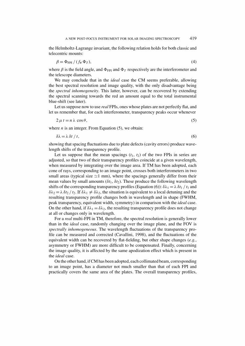
Once the optimum ratio has been found, the best spacing can be looked for. To thisend, recall that the spectral resolving power (R) is a relevant instrumental parameterdepending on the spacing. For a single ideal interferometer in CM (Equation (1)):

R= λ/FWHMCM = [λ (1 − R)]−1 2πμt R1/2. (14)

Two opposing requirements must be therefore envisaged: because with increasingspacing both parasitic light and spectral resolving power increase (Section 2.3 andEquation (14)), the best spacing will be a compromise between a low P and a highR. Moreover, because with increasing wavelength both parasitic light and spectralresolving power decrease (Section 2.3 and Equation (14)), these two quantities havebeen respectively calculated at the shortest (580 nm) and at the longest (860 nm)wavelengths used, while the broadening of the transparency profile, due to cavityerrors, has been evaluated as described in Section 4.1. Finally, R and P have beenplotted in Figure 3 versus the spacing of the thickest FPI, for R varying from0.90 to 0.95. This figure seems to suggest that the highest coating reflectivity isthe best choice, providing the highest R and the lowest P . We have to consider,however, that with the increasing reflectivity, the overall maximum transmittance ofthe two interferometers (Equations (11) and (13)) and the image quality (Ramsay,

A NEW POST-FOCUS INSTRUMENT FOR SOLAR IMAGING SPECTROSCOPY 425

Figure 3. Abscissae: spacing of the thickest FPI. Ordinates: spectral resolving power (R) at 860 nm

and parasitic light (P) at 580 nm, for a plate reflectivity ranging from 0.90 to 0.95, by steps of 0.01.

Dashed lines refer to a reflectivity of 0.93.

1969) decrease, while the ghost relative intensity increases (see Section 2.5). Thissuggests using the less reflective coating, compatible with the spectral resolutionand the parasitic light.

Going back to Figure 3, it may be seen that, assuming R = 0.93 and t = 2.3 mm(vertical dashed line), a spectral resolving power R ≥ 200 000 and a parasitic lightP ≤ 2.5% are obtained.

Therefore, a pair of interferometers with spacings t = 2.300 (FPI 1) and0.637 mm (FPI 2) and a coating reflectivity R = 0.93 have been chosen, as thebest compromise between transparency, ghosts, parasitic light, image quality andspectral resolution.

426 F. CAVALLINI

TABLE II

Fabry-Perot Interferometer Characteristics.

Manufacturer IC Optical Systems

Type ET50 FS

Clear aperture 50 mm

Plate spacings 2.300, 0.637 mm

Wedge angle 20′

Coating Multilayer broadband

Wavelength range 580 – 860 nm

Reflectance 0.93

Absorption coefficient 0.002

Cavity errors (nominal) λ/150 (after coating)

Setting time � 20 ms

The primary characteristics of both interferometers are shown in Table II.

2.5. THE GHOSTS

Up to this point, we have implicitly supposed that both interferometers are used inaxial-mode (the plates normal to the optical axis), and we have not considered theeffects of the reflected radiation. In reality, a collimated raybundle incident on aFPI produces both a transmitted and a reflected beam. The transmission profile ofan ideal interferometer has been already given (Equation (10)), while its reflectionprofile is (Vaughan, 1989):

Ri (λ) = (1 − A) [1 − A(λ)] + A(λ) A2 R/(1 − R)2. (15)

Both in classic and in telecentric mounts, the inter-reflections between two inter-ferometers in series produce ghost images at the final focal plane that must beaccuratly evaluated. Let us consider therefore an IF with a transparency profile TIF,followed (or preceded) by two FPIs with transparency and reflectivity T1, R1 andT2, R2, respectively. If the relative distance between the interferometers is muchlarger than their plate spacings, the FPIs can be considered “decoupled” (Steel,1967) and incoherent addition of intensities may be assumed for the inter-reflectedradiation. In this case it is easy to show that the ghost profile G(λ) is given by

G(λ) = TIF(λ) T1(λ) T2(λ) [1/(1 − R1(λ)R2(λ) − 1)]. (16)

Moreover, if T (λ) is the transparency profile of the principal image (the first trans-mitted one), we have (Equation (8)):

T (λ) = TIF(λ) T1(λ) T2(λ). (17)

A NEW POST-FOCUS INSTRUMENT FOR SOLAR IMAGING SPECTROSCOPY 427

By comparing G(λ) and T (λ), it may be seen that the former dominates the lat-ter everywhere, save near the transparency peak, producing extended wings, thatsignificantly reduce the spectral resolution.

Moreover, if we observe an object with a flat spectrum, the flux associated withits image is proportional to the equivalent width of the instrumental profile, definedas

W =∫ λ2

λ1

T (λ) dλ, (18)

where λ1 = −2 nm and λ2 = 2 nm (Section 2.3). Therefore, if �G and �P are thefluxes corresponding to the ghosts and to the principal image respectively, we have:

�G/�P =∫ λ2

λ1

G(λ) dλ

/ ∫ λ2

λ1

T (λ) dλ =WG /WP . (19)

It may be shown that �G/�P increases with decreasing wavelength and increasingreflectivity, and that, in particular, for the two IBIS interferometers (R = 0.93),�G/�P changes from 0.32 (860 nm) to 0.52 (580 nm). We may conclude thereforethat the inter-reflections so seriously affect both the imaging and the spectroscopicquality, that it is mandatory to eliminate them or to reduce their effects to acceptablevalues.

A generally adopted solution consists in tilting one or both interferometers ata small angle, sufficient to allow the ghost images to clear the field (Loughhead,Bray, and Brown, 1978; Kentischer et al., 1998; Koschinsky, Kneer, and Hirzberger,2001). If both interferometers are equally rotated around the same axis, but inopposite directions, the required tilt angle is

α ≥ 1/(4 f#). (20)

Since generally large f# are used ( f# � 100), small tilt angles are required(α � 0.1◦), sufficient however to produce serious secondary effects.

In CM a consequence of the tilt is a detuning of the two FPIs, increasing fromthe tilt axis towards the edge of the field, which produces an increasing asymmetryand a decreasing W of the instrumental profile. In comparison with the no-tilt case,the transparency is the same along the tilt axis, but decreases normally to this,reaching a minimum at the extremes of the perpendicular diameter. This producesan inhomogeneous darkening of the FOV, resulting in a general loss of instrumentaltransmittance, which can be evaluated as

D(λ) =[∫

FOV

W dS −∫

FOV

WT(P) dS

] / ∫FOV

W dS, (21)

where dS is a surface element, andW ,WT (P) respectively are the equivalent widthwithout and with tilt, this latter depending on the image point considered (P). ForIBIS ( f# = 110) a tilt angle α = ± 0.13◦ should be adopted to avoid the ghosts;

428 F. CAVALLINI

this would produce an overall darkening, decreasing with increasing wavelength,ranging from D = 0.51 (580 nm) to D = 0.39 (860 nm).

In TM and in the ideal case, each cone of rays finds instead the same detuningsituation in crossing the two tilted FPIs. The instrumental profile is therefore thesame at each image point, but it is strongly asymmetric and with a reduced equivalentwidth. The result is a homogeneous darkening of the field, equivalent to an overallloss of instrumental transmittance, which, in this case, can be computed as

D(λ) = (W − WT) /W. (22)

Evaluating Equation (22) for IBIS, we find again D = 0.51 (580 nm) and D = 0.39(860 nm), confirming that, for the same tilt angle, the loss of flux through thetwo FPIs does not change for different optical mounts. In reality, from the opticalpoint of view, the situation at the pupil, in TM, is the same as that at the image,in CM, and vice versa. In TM, however, due to the inhomogeneous darkeningof the pupil, the tilt not only produces an asymmetric instrumental profile and aloss of instrumental transparency, but also an apodization effect, causing a furtherasymmetric broadening of the instrumental point spread function.

We may conclude therefore that, if the tilting is an effective method to eliminatethe ghost images, it generally produces such serious secondary effects, both inclassic and in telecentric mounts, that a different solution must be looked for.

Going back to the Equations (16) and (17), it may be shown that, if the IF doesnot follow or precede the two FPIs, but it is placed between them:

G(λ) = TIF(λ) T1(λ) T2(λ){ [

1 − T 2IF(λ)R1(λ)R2(λ)

]−1 − 1}

(23)

and

T (λ) = TIF(λ) T1(λ) T2(λ). (24)

By inserting Equations (23) and (24) in Equation (19), and calculating again �G/�P

for different τIF values of the IF transparency peak, we find that, for τIF = 0.30,�G/�P ≤ 0.015 over all the useful wavelength range. Moreover, in this case, bycomparing Equation (23) and Equation (24), it may be seen that G(λ) is everywherenegligible in comparison with T (λ).

Because τIF � 0.30 is the typical peak transparency of the narrow-band IFsselected as order sorters for IBIS (see Table I), the solution finally adopted was toinsert the filters between the two interferometers (Cavallini et al., 2000). In this waythe ghost effects on the imaging and on the spectroscopy are reduced to acceptablevalues, and both interferometers can be used in axial-mode, without affecting theshape of the instrumental profile and, most importantly, without any transparencyloss.

A NEW POST-FOCUS INSTRUMENT FOR SOLAR IMAGING SPECTROSCOPY 429

3. The Instrument

3.1. THE PRINCIPAL OPTICAL PATH

IBIS has been installed at the DST on an optical bench, feed by a high-orderAO system. This essentially is formed by a tip/tilt corrector, a Shack-Hartmannwavefront sensor (76 subapertures, 2500 frames s−1), and a deformable mirror (97actuators) described by Rimmele et al. (2004).

Figure 4 schematically represents the IBIS layout, where the principal opticalpath is shown by the solid line. At the exit of the high-order AO, the telescopeprimary image is at infinity and a pupil image is formed near the first foldingmirror m1, at the focus of the transfer lens L0. This lens and two further mirrors(m2, m3) form the solar image on the field stop (FS) of the instrument, 21.3 mmin diameter, corresponding to 80′′ on the Sun. Three lenses (L1, L2, L3) and afolding mirror (M1) successively collimate the solar and the pupil image. AfterL3, the two FPIs, used in axial-mode and in classic mount and, between them, afilter wheel (FWH) carrying a hole, a dark slide and five interference filters (seeTable I). To avoid unwanted effects from interferometer tilts (see Section 2.5), theorthogonality to the optical axis must be secured for both FPIs. To accomplish this,each interferometer can be rotated on two perpendicular axes and it is mounted onan independent translating stage, allowing it to be removed from the optical path.Before any observing run, with the sunlight feeding the instrument, a pair of pelliclebeamsplitters (BS2) are inserted into the principal optical path. The first one is at45◦ with respect to the optical axis, while the second one is perpendicular to itand at the focus of the L2 lens, where two images are formed: the first one by L2(direct image), the second one by L3, after reflection on one of the FPIs (reflectedimage). Both of these images are reflected by the first pellicle beamsplitter anda folding mirror (M4) onto a TV camera (TV2). The procedure for determiningthe interferometer perpendicularity is as follows. First, FPI 1 is removed from theoptical path, the open position is selected in the filter wheel, and FPI 2 is rotatedaround the two allowed axes, so as to overlap the direct and the reflected image.Then, FPI 1 is reinserted into the optical path and the same procedure is repeated.This method allows us to adjust the perpendicularity of each interferometer to theoptical axis with an accuracy of ±10′′. Moreover, a diaphragm D, placed in front ofFPI 1 and centered on the incoming beam (just a few millimeters larger in diameter)can be used as reference for the position of the optical axis on the interferometerplates.

Going back to Figure 4, a fourth lens (L4) and two further folding mirrors (M2,M3) form a solar image, 6.85 mm in diameter, on a CCD camera (CCD 1) (seeTable IV). As the overall FOV is 80′′ and the FWHM of the telescope point spreadfunction is 0.19′′ at 580 nm, 418 is the maximum number of resolved elements.Assuming two pixels per resolved element, a detector with at least 836 × 836 pixelsis required. In our case the solar image is inscribed in a square area measuring

430 F. CAVALLINI

Figure 4. Schematic drawing of the instrumental layout. The solid line represents the principal optical

path, while the secondary ones are shown by dashed lines. The moveable optical components, which

can be inserted or extracted from the optical path, are represented as transparent objects. The meaning

of the labels is as follows. BS: beamsplitter; BST: beam steering; CCD: CCD camera; ES: electronic

shutter; FPI: Fabry-Perot interferometer; FS: field stop; FWH: filter wheel; HL: halogen lamp; L:

lens; LW: lens wheel; M, m: mirror; PMT: photomultiplier; RL: relay lenses; TV: TV camera; W:

window.

1007 × 1007 pixels on a CCD with 1024 × 1024 pixels. This implies an image scaleof 0.08′′ pixel−1 (at least 2.4 pixels per resolved element), such as to completelyexploit the telescope spatial resolution.

A NEW POST-FOCUS INSTRUMENT FOR SOLAR IMAGING SPECTROSCOPY 431

3.2. THE REFERENCE PATH

This secondary path originates from two beamsplitters (BS1) placed between L1and L2 (see Figure 4), in a space where the solar image is at infinity. Each of themis a BK7 plane-parallel window, anti-reflection coated on both surfaces, reflectinga small amount of the incoming light (≤ 0.5%) to a TV (TV5) and to a CCDcamera (CCD 2) (see Table IV) through two folding mirrors (M12 and M13). Anelectronic shutter (ES), placed between the two beamsplitters in a pupil space,simultaneously controls the exposure time for CCD 1 and CCD 2. The thickness ofeach beamsplitter (12.7 mm) is such that the secondary pupil image, coming fromits rear surface, is sufficiently far from the principal one to be eliminated by meansof a suitable diaphragm. Both TV5 and CCD 2 are equipped with a photographiczoom lens, allowing the adjustment of the image scale, an interference filter (λ =720 nm, FWHM �10 nm) and a pair of linear polarizers, to adjust the light level.TV5, continuously showing the selected solar region, is used to monitor the solarand atmospheric conditions. CCD 2 allows one to take, simultaneously with CCD 1,broad-band images of the same FOV, which can be used as a transparency referenceand/or for post facto procedures, to correct the seeing effects.

3.3. THE TUNING PATH

The initial tuning between the two interferometers and the selected interferencefilters is obtained by using a halogen lamp (HL). Its output is kept constant to betterthan 1% by a light intensity control system for a sufficiently long time such that noother reference is required. The goal is to faithfully reproduce the optical situationwhen the Sun is observed, but with a source with a flat spectrum. To this purpose,the lamp light is concentrated on a flashed opal diffuser, and a suitable system ofrelay lenses (RL) provides an image of the diffuser with the same size and f# asthe solar one produced by L2. This image can be put on the L3 focus by meansof a fixed (M6) and of a moveable (M8) folding mirror. The perpendicularity ofthe lamp light to the interferometers is then verified by inserting in the optical pathBS3, a pair of pellicle beamsplitters identical to BS2 (see Section 3.1). The directand the reflected images can be seen thanks to the folding mirror M5 and the TVcamera TV3, while the position of the beam on the diaphragm D is shown by TV4,through M10 and M11, as a bright ring. By adjusting the orientation of M6 andM8, it is possible to simultaneously overlap the two images and to make the ringsymmetrical, securing in this way the perpendicularity and the centering of theincident beam. Once these two conditions are verified, the lenses L3 and L4, themirrors M2 and M14, and the moveable mirror M9 finally form an image of thediffuser on the photochatode of a photomultiplier (PMT). Tuning is then performedby keeping FPI 2 at a fixed voltage and measuring the PMT signal, while scanningFPI 1. The voltage where the maximum signal is found corresponds to a tuningsituation, namely to the coincidence of one interference order of FPI 1 with one of

432 F. CAVALLINI

FPI 2. A further scanning, performed with both interferometers tuned, allows oneto find the peak transparency of the selected interference filter.

3.4. THE LASER PATH

This secondary optical path is used to verify and to adjust the parallelism of theinterferometer plates. To this purpose, the beam of a frequency-stabilized He-Nelaser is sent through a beam steering system (BST) near the edge of a circularrotating diffuser. The result is a small bright spot, with a rapidly changing specklepattern, which simulates a monochromatic incoherent source. This spot illuminates,at short distance, a second flashed opal diffuser (� 8 mm in diameter), an image ofwhich can be then put, by means of the moveable mirror M7, at the focus of the L3lens.

The two lenses L3 and L4, the fixed mirror M2, and the moveable mirror M9finally send the laser light to LW. This is a wheel, carrying three different lenses,respectively forming on TV1 an image of the diffuser and of the FPI 1 and FPI 2plates.

As a first step, FPI 2 is removed from the optical path and a suitable lens isselected on the LW, showing on TV1 the diffuser image. Its monochromatic light,crossing FPI 1, produces a ring system, the inner part of which can be seen withsuperimposed the diffuser circular edge. By adjusting M7 to center the ring systemon the diffuser contour, normal incidence of the laser light on the interferometerplates is obtained. By selecting a suitable lens on the LW, TV1 shows the FPI 1plates, lighted by the laser. Due to the wavelength fluctuations of the transparencyprofile produced by spacing and parallelism errors, the plate image generally showsboth random and systematic brightness inhomogeneities. By changing the appliedvoltage, so that one interference order moves back and forth in wavelength on thelaser line, and adjusting, at the same time, the parallelism conditions to obtainan image changing as homogeneously as possible, the best parallelism condition isfinally obtained. The same procedure can be then repeated for FPI 2, by exchangingthe two FPIs on the optical path, and by selecting a third suitable lens on the LW.

4. The Expected Instrumental Characteristics

4.1. THE SPECTRAL RESOLVING POWER

To correctly calculate the spectral resolving power, the broadening of the instru-mental profile, due to the cavity errors, must be properly evaluated. To this purpose,if incoherent addition of intensities is assumed, the transparency profile can be ob-tained as the convolution between that of an ideal FPI and the distribution functionof the wavelength shifts due to the plate defects Vaughan, 1989). The peak-to-peak

A NEW POST-FOCUS INSTRUMENT FOR SOLAR IMAGING SPECTROSCOPY 433

value of these, expressed as λ0/p (λ0 = 632.8 nm, p = 150 after coating), is the onlyinformation provided by the manufacturer. We conservatively assumed p = 100 andsupposed the cavity errors as being due to a symmetric parabolic nonuniformity(see Section 2.1). The corresponding shift distribution, in this case, is a rectangularfunction, with a width λλ0/(pt). Under these hypotheses, the overall instrumentalprofile can be calculated and a spectral resolving power is found, ranging from200 000 to 270 000.

4.2. THE EXPOSURE TIME AND THE TEMPORAL RESOLUTION

To evaluate the expected exposure time (a relevant instrumental parameter if highspatial resolution is wanted), let us estimate firstly the photoelectron flux on thedetector. This may be written as

� (e− s−1 pixel−1) = H 2 D2 τT τO τIF λ fλ Qλ W e−Kλ/ cos z (h c α2)−1, (25)

with the following meaning of the symbols. H (arcsec pixel−1): image scale onthe detector; D (cm): diameter of the telescope entrance pupil; τT, τO and τIF:transparency of the telescope, of the IBIS optics and of the interference filter,respectively; fλ (erg cm−2 s−1 nm−1): solar flux outside the Earth’s atmosphere inthe continuum between the lines; Qλ (e− photon−1): detector quantum efficiency;W (nm): equivalent width of the instrumental profile; Kλ: exponential absorptioncoefficient of the Earth’s atmosphere; z (degrees): Sun zenith distance; α (arcsec):solar angular diameter, and h c/λ (erg photon−1): photon energy.

If we demand a signal to noise ratio S/N ≥ 100, a minimum of 104 e− pixel−1

is required, namely an exposure time

t (ms) ≥ 107/�. (26)

� has been then evaluated by taking fλ and Kλ from Allen (1985), and Qλ from thequantum efficiency curve of the detector (Kodak KAF-1400). Moreover, D = 76.2cm (DST entrance pupil diameter), τIF = 0.30, H = 0.08′′ pixel−1 (see Table IV),and z = 45◦ have been assumed. To evaluate τO, the following expression has beenthen used:

τO = T 4L T 2

BS T 8W T 2

P1T 2

P2R3

M , (27)

where TL = 0.988, TBS = 0.981, TW = 0.989, TP1= 0.986, and TP2

= 0.983 respec-tively are the transparency of each lens, beamsplitter, window, first and secondplate of the IBIS FPIs. All of the surfaces of these optical elements have an anti-reflection (AR) coating, optimized in the range 580 – 860 nm. Its reflectivity, aswell as the glass internal absorption, have been considered in calculating the overalltransparency. Moreover, RM = 0.980 has been assumed for the reflectivity of eachmirror (protected Ag). Inserting these values in Equation (27), we find τO = 0.742.Finally, the shortest allowed exposure times (ti ) have been evaluated by means

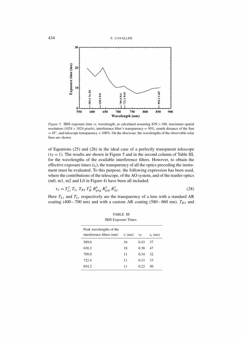
434 F. CAVALLINI

Figure 5. IBIS exposure time vs. wavelength, as calculated assuming S/N = 100, maximum spatial

resolution (1024 × 1024 pixels), interference filter’s transparency = 30%, zenith distance of the Sun

= 45◦, and telescope transparency = 100%. On the abscissae: the wavelengths of the observable solar

lines are shown.

of Equations (25) and (26) in the ideal case of a perfectly transparent telescope(τT = 1). The results are shown in Figure 5 and in the second column of Table III,for the wavelengths of the available interference filters. However, to obtain theeffective exposure times (te), the transparency of all the optics preceding the instru-ment must be evaluated. To this purpose, the following expression has been used,where the contributions of the telescope, of the AO system, and of the tranfer optics(m0, m1, m2 and L0 in Figure 4) have been all included:

τT = T 2Ls TLc TBS T 2

W R6pAg R2

pAl R3Al. (28)

Here TLs and TLc respectively are the transparency of a lens with a standard ARcoating (400 – 700 nm) and with a custom AR coating (580 – 860 nm). TBS and

TABLE III

IBIS Exposure Times.

Peak wavelengths of the

interference filters (nm) ti (ms) τT te (ms)

589.6 16 0.43 37

630.2 18 0.38 47

709.0 11 0.34 32

722.4 11 0.33 33

854.2 11 0.22 50

A NEW POST-FOCUS INSTRUMENT FOR SOLAR IMAGING SPECTROSCOPY 435

TW respectively are the transparency of each beamsplitter and window, while RpAg,RpAl and RAl are the reflectivity of mirrors respectively protected Ag, protected Al,and unprotected Al.

The calculated τT and te values are reported in Table III, showing that the lowtransparency of the optics in front of the instrument sensibly increases the exposuretimes. In any case, the expected te, ranging from 32 and 50 ms, seems to be suffi-ciently short to freeze most of the seeing. Finally, the temporal resolution can beevaluated by considering the time required for the wavelength setting (� 20 ms),the exposure (≤50 ms), the readout (300 ms at 5 MHz), and the storing (� 30 ms)of each image (1024 × 1024 pixels). An acquisition rate of �2.5 frames s−1 can betherefore expected.

4.3. THE TUNING AND THE WAVELENGTH STABILITY

As the instrument is essentially formed by two FPIs in series, their wavelengthstability is critical, not only to warrant a good reproducibility of the selected spectralpoints on long observing runs, but also to avoid any detuning which could changethe shape of the resulting instrumental profile. A detuning of 0.28 pm at 580 nm hasbeen assumed as the maximum permitted, producing an asymmetry of � 0.1 pmand a decrease of � 0.5% of W , namely of the overall instrumental transmittance.At longer wavelengths less strict requirements can be adopted.

On the other hand, the wavelength stability of each interferometer dependsonly on the stability of its cavity optical length (μt in Equation (5)). For each ofthe adopted FPIs, the plate parallelism and geometrical spacing (t) are controlledby a close-loop electronic system (CS100), using five capacitance sensors andthree piezo-electric actuators. The CS100, however, is sensitive to changes of thedielectric constant of the air and to thermal effects of the capacitor pillars and ofsome electronic components. Moreover, the refractive index (μ) of the air betweenthe plates changes, due to any variation of the ambient pressure, temperature, orhumidity. To eliminate the environmental effects on the capacitance sensors and onthe cavity optical length, each interferometer is enclosed in a sealed cell.

The temperature sensitivity of the capacitor pillars produces a drift of0.28 pm ◦C−1 for FPI 1 and 0.27 pm ◦C−1 for FPI 2. This effect has been reducedby means of a thermostatic system, similar to that used for the IPM FPI (Cavallini,1998), able to mantain each interferometer at � 38 ◦C within ± 5×10−3 ◦C. In thisway a maximum drift of ±1.4×10−3 pm (for both positive or negative shifts), anda maximum detuning of 2.8×10−3 pm (for opposite shifts) have been obtained.

Moreover, the CS100 temperature sensitivity (50 pm ◦C−1), producing a driftof 1.3×10−2 pm ◦C−1 for FPI 1 and 4.6×10−2 pm ◦C−1 for FPI 2, has beencompensated by means of a rough temperature control (± 0.1 ◦C), obtained bycontrolling the speed of the cooling fan of each CS100. In this way the maximum

436 F. CAVALLINI

drift and the maximum detuning have been respectively reduced to ± 3.0×10−3 pmand 5.9×10−3 pm.

The largest source of detuning is however the CS100 digital resolution (12 bits),allowing the change of the plate spacing by discrete steps of 0.49 nm. Due to thedifferent spacings of the two FPIs, the corresponding wavelength steps (λ) are(Equation (6))

λ1/λ2 = t2/t1. (29)

This implies that the minimum wavelength step (see Table IV) is imposed by theinterferometer with the smallest spacing (FPI 2), while the maximum possibledetuning is one half of the FPI 1 minimum wavelength step, namely 6.2×10−2 pmat 580 nm. This is the worst situation, when the peak wavelength of the FPI 2 orderused is in the middle of two admitted wavelength positions of one FPI 1 interferenceorder.

Therefore, the maximum expected detuning, when all of the possible effectsare considered, amounts to 7×10−2 pm, well below the maximum admitted valueof 0.28 pm, while the maximum expected drift amounts to ± 4.4×10−3 pm, or± 2.3 ms−1, in velocity units.

However, some tests of long-term wavelength stability, performed on a similarinterferometer with an equivalent thermostatic system Cavallini 1998), showed alarger drift, amounting to � 10 ms−1 in 10 hours, which has been conservativelyassumed also for IBIS. This is equivalent to assuming that all of the thermal insta-bilities evaluated before amount to 2×10−2 pm for each FPI. In this case, therefore,the maximum expected detuning, when the CS100 digital resolution is also consid-ered, amounts to 0.1 pm, while the maximum expected drift amounts to ±0.01 pm,or ±5.2 ms−1, in velocity units. Both drift and detuning are larger under this as-sumption, but small in absolute value; the detuning, in particular, is still below themaximum admitted value of about a factor three.

Finally, the wavelength stability of the interference filters must be also consid-ered. To reduce the parasitic light and to avoid an excessive loss of transparency, anarrow range (λ) around the peak wavelength of each interference filter is used,where the transparency is larger than 85% of the peak. This implies a λ � 0.2nm for the filters with a 0.3 nm passband, and a λ � 0.3 nm for those with a0.5 nm passband (Equation (12)). Since the maximum transparency gradient is0.7% pm−1 at ± 0.1 nm from the peak wavelength of the filters with a 0.3 nm pass-band (Equation (12)), and since they have a temperature sensitivity of � 2 pm ◦C−1,the filter wheel has been closed with two glass windows and the temperature in-side has been stabilized within ± 0.1 ◦C. This achieves a wavelength stability of± 0.2 pm of the interference filters, corresponding to a maximum transparencyvariation of ± 0.14%.

A NEW POST-FOCUS INSTRUMENT FOR SOLAR IMAGING SPECTROSCOPY 437

TABLE IV

IBIS Characteristics.

Wavelength range 580 – 860 nm

Spectral resolving power 200 000 – 270 000

Wavelength drift ≤ 10 ms−1 in 10 h

Wavelength blue-shift on 6 – 9 pm

the image plane (radial)

Field of view (circular) 80′′

Wavelength setting time � 20 ms

Minimum wavelength step 0.45 – 0.66 pm

Monochromatic camera Roper PentaMAX

1317 × 1035 square pixels

6.8 μm in size.

Dyn. range: 12 bits

Data rate: 5 MHz

Broad band camera Dalsa CA-D7-1024T

1024 × 1024 square pixels

12 μm in size.

Dyn. range: 12 bits

Data rate: 10 MHz

Image scale 0.08′′ pix−1 (2.4 – 3.6 pix/r.e.)

Exposure time 32 – 50 ms

(S/N = 100 in the solar continuum) (1024 × 1024 pixels)

Acquisition rate including: � 2.5 frames s−1 (1024 × 1024 pixels);

wavelength setting, � 4 frames s−1 (binning 2 × 2)

exposure, frame reading,

storing

5. Summary

The IBIS instrumental characteristics, shown in Table IV, seem to meet the initialrequirements well. The spectral and the temporal resolution are satisfactory, as wellas the useful wavelength range, the FOV, and the wavelength stability. Concerningthe spatial resolution, the image scale allows a suitable sampling and the exposuretime is sufficiently short to use post facto image restoring techniques. At first glance,the monochromatic images seem of good quality, showing, when compared withsimultaneously taken broad-band images, a comparable spatial resolution and onlya slight decrease in contrast. However, without knowing the real cavity errors and

438 F. CAVALLINI

their spatial distribution, it is difficult to quantitatively evaluate the effective imagequality. This latter, as well as other instrumental characteristics which need to bedirectly measured, will be the subject of a following paper.

Acknowledgements

Thanks are due to Dr. C. Baffa for having written the first version of the controlsoftware for the instrument, afterwards developed and improved by Dr. K. Reardon;to G. Falcini and to S. Paloschi for having built the mechanical structure and theelectronic controls; to T. Grisendi and F. Fabiani for assistance in assembling andtesting the instrument; to Prof. A. Egidi, Prof. S. Cantarano and Prof. F. Berrilliwho provided the software for the CCD acquisition system. Thanks are also dueto Dr. A. Falchi, Prof. R. Falciani, and Dr. G. Cauzzi for their suggestions andencouragement.

IBIS was built with the contribution of the INAF – Osservatorio Astrofisico diArcetri, the Universita di Firenze, the Universita di Roma “Tor Vergata”, and theMinistero dell’Universita e della Ricerca Scientifica.

Since June 2003 this instrument is installed at the Dunn Solar Telescope of theNational Solar Observatory, operated by the Association of Universities for Re-search in Astronomy, Inc. (AURA), under cooperative agreement with the NationalScience Foundation. We are grateful to the observing staff of the DST for theircontinued assistance in the installation phase.

References

Allen, C.W.: 1985, Astrophysical Quantities. The Athlon Press, London.

Beckers, J.M.: 1998, Astron. Astrophys. Suppl. 129, 191.

Bendlin, C. and Volkmer, R.: 1995, Astron. Astrophys. Suppl. 112, 371.

Bendlin, C., Volkmer, R., and Kneer, F.: 1992, Astron. Astrophys. 257, 817.

Cavallini, F.: 1998, Astron. Astrophys. Suppl. 128, 589.

Cavallini, F., Berrilli, F., Cantarano, S., and Egidi, A.: 2000, in A. Wilson (ed.), The Solar Cycle andTerrestrial Climate, ESA Publications Division, Noordwijk, ESA SP-463, p. 607.

Kentischer, T.J., Schmidt, W., Sigwarth, M., and von Uexkull, M.: 1998, Astron. Astrophys. 340,

569.

Koschinsky, M., Kneer, F., and Hirzberger, J.: 2001, Astron. Astrophys. 365, 588.

Loughhead, R.E., Bray, R.J., and Brown, N.: 1978, Appl. Opt. 17, 415.

Neidig, D., Wiborg, P., Mozer, J., Dalrymple, N., Dunn, R., Gregory, S., and Gullixson, C.: 2003,

Bull. Am. Astron. Soc. 35, 848.

Netterfield, R.P. and Ramsay, J.V.: 1974, Appl. Opt. 13, 2685.

Ramsay, J.V.: 1969, Appl. Opt. 8, 569.

Ramsay, J.V., Kobler, H., and Mugridge, E.G.V.: 1970, Solar Phys. 12, 492.

Rimmele, T.R., Richards, K., Hegwer, S.L. et al.: 2004, Proc. SPIE 5171, 179.

Steel, W.H.: 1967, Interferometry, Cambridge University Press, Cambridge, p. 125.

A NEW POST-FOCUS INSTRUMENT FOR SOLAR IMAGING SPECTROSCOPY 439

Tritschler, A., Schmid, W., Langhans, K., and Kentischer, T.: 2002, Solar Phys. 211, 17.

Vaughan, J.M.: 1989, The Fabry-Perot interferometer: History, Theory, Practice and Applications.

Adam Hilger, Bristol and Philadelphia.

von der Luhe, O. and Kentischer, T.J.: 2000, Astron. Astrophys. 146, 499.