UPTEC F10049

Examensarbete 30 hpAugusti 2010

Ice navigation with ice compression in the Gulf of Finland

Niklas Berg

Teknisk- naturvetenskaplig fakultet UTH-enheten

Besöksadress: Ångströmlaboratoriet Lägerhyddsvägen 1 Hus 4, Plan 0

Postadress: Box 536 751 21 Uppsala

Telefon:018 – 471 30 03

Telefax: 018 – 471 30 00

Hemsida:http://www.teknat.uu.se/student

Abstract

Ice navigation with ice compression in the Gulf ofFinland

Niklas Berg

Safe winter navigation is a hot topic. Not only is the traffic density increasing but theenvironmental considerations are also getting bigger. An oil leakage from a big oiltanker can be of catastrophic proportions in the wrong area and more trafficincreases the risk of an accident. A project that aims for safer winter navigation isSafeWIN. The aim of this project is to develop a forecasting system for compressiveice and thus make winter navigation safer. This thesis is part of above mentioned project and aims to investigate what influenceice compression and ice class has on winter navigation. Vessels are exclusivelyAFRAMAX size tankers sailing on Primorsk in the Gulf of Finland during 2006. Transitdata comes from AIS tracks recorded by the Swedish Maritime Administration. Adatabase with tanker transits has been created and this information is the source forthe studies in this thesis. Included in the database are wind data, ice particulars andtransit information such as speed, and time at different activities during the transit.Average values for a transit has been investigated for comparison and to get a pictureof an average transit. Velocity, waiting time and time with assisting icebreaker are parameters that arebelieved to show how a tanker performs in winter navigation. These parameters arecompared with ice compression and ice class separately to see if there is acorrelation. Ice compression has also been investigated for correlation towards windforce to see if stronger wind generates stronger compression. Using the velocity in different ice compressions an estimate of ice resistance that stemfrom ice compression has been extracted by means of Lindqvist’s formula.

Sponsor: Stena Rederi ABISSN: 1401-5757, UPTEC F10049Examinator: Tomas NybergÄmnesgranskare: Kjartan HalvorsenHandledare: Göran Liljeström

1

Acknowledgements

This thesis has been carried out in cooperation with Stena Rederi AB. They have helped me

with a lot of things. Getting access to the information from various sources where they have

contacts and given a helping hand whenever I needed it. Many thanks for that.

Göran Liljeström at Stena Teknik has been my main contact at Stena and has been a great

support. Thank you for all your help.

Secondly Fredrik Efraimsson and David André at Stena Teknik have helped me with various

parts during this thesis. Thank you for all your comments and material.

Kjartan Halvorsen, my academic supervisor, thank you for steering me in the right direction

and for all academic input.

I would like to thank Polina Soloshchuk at Hydrometeorological Center of St.-Petersburg who

helped me with the Russian ice charts and weather information.

At last I would like to direct my gratitude to everyone else that helped me make this thesis

possible.

Stockholm, June 2010

Niklas Berg

2

3

List of nomenclature

L - Ship length

B - Vessel width

T - Vessel draft

E - Elastic modulus

σb - Bending strength of ice

ψ - Angle between normal of surface and vertical vector( )

α - Water line entrance angle

φ - Stem angle

μ - Friction coefficient

δp - Density difference between ice and water

ρw - Density of water

g - Gravitational constant

Hice - Ice thickness

Fv -Force acting on ice

List of abbreviations

Hog - Island of Hogland

Priin -Point were vessels inbound for Primorsk turn north east. See chapter 3.2.1. Pri -Port of Primorsk

GoF -Gulf of Finland

TSS -Traffic separation scheme

AIS -Automatic identification system

AFRAMAX- Size of vessel, Deadweight under 120000 tones and breadth more than 32.31 m

MCR - Maximum continuous revolution

NCR - Normal continuous revolution

Nm - Nautical miles

4

Contents Acknowledgements .................................................................................................................... 1

List of nomenclature ................................................................................................................... 3

List of abbreviations ................................................................................................................... 3

1. Introduction ........................................................................................................................ 9

1.1 Background .................................................................................................................. 9

1.2 Objective of the study .................................................................................................. 9

1.3 Method ....................................................................................................................... 10

1.4 Limitations ................................................................................................................. 10

2. Winter navigation ............................................................................................................. 11

2.1 General about winter navigation in the Baltic ........................................................... 11

2.1.1 Finnish Swedish ice class ................................................................................... 11

2.2 SafeWIN .................................................................................................................... 12

2.3 Components affecting ice resistance ......................................................................... 12

2.3.1 Crushing at the stem ........................................................................................... 12

2.3.2 Breaking by bending .......................................................................................... 13

2.3.3 Submersion ......................................................................................................... 13

2.3.4 Speed .................................................................................................................. 13

2.3.5 Lindqvist’s complete formula ............................................................................ 13

2.4 Ice compression ......................................................................................................... 14

2.5 Ice situation 2006 in the Gulf of Finland ................................................................... 14

2.6 Gulf of Finland in a navigational aspect .................................................................... 15

2.6.1 Route to Primorsk ............................................................................................... 16

3. Database ........................................................................................................................... 18

3.1 Raw material .............................................................................................................. 18

3.1.1 Adveto Aecdis-2000 ver. 2009-09-01 ................................................................ 18

3.1.2 Automatic Identification System data ................................................................ 18

3.1.3 Ice charts ............................................................................................................ 19

3.1.4 Wind data ........................................................................................................... 21

3.2 Explanation of database ............................................................................................. 21

3.2.1 Areas in the Gulf of Finland ............................................................................... 21

3.2.2 Ice classes ........................................................................................................... 22

3.2.3 Ice particulars ..................................................................................................... 22

3.2.4 Icebreaker ........................................................................................................... 23

3.2.5 Transit particulars ............................................................................................... 23

5

3.2.6 Average speed .................................................................................................... 24

3.2.7 Distance .............................................................................................................. 24

3.2.8 Ice edge longitude .............................................................................................. 24

3.2.9 Weather .............................................................................................................. 24

3.2.10 Extra material ..................................................................................................... 24

3.3 Procedure ................................................................................................................... 24

4. Analysis ............................................................................................................................ 26

4.1 Traffic pattern ............................................................................................................ 26

4.2 Ice class ...................................................................................................................... 26

4.3 Wind and ice compression correlation ...................................................................... 26

4.4 Ice compression and transit particulars ..................................................................... 27

4.4.1 Speed .................................................................................................................. 27

4.4.2 Waiting time ....................................................................................................... 27

4.4.3 Icebreaker time ................................................................................................... 28

4.5 Technical estimate of ice resistance originating from ice compression .................... 28

5. Results .............................................................................................................................. 29

5.1 Traffic pattern ............................................................................................................ 29

5.1.1 Icebreaker assistance .......................................................................................... 29

5.1.2 Waiting and stop ................................................................................................. 29

5.1.3 The Mean transit ................................................................................................. 30

5.1.4 Average speed .................................................................................................... 31

5.2 Ice classes .................................................................................................................. 32

5.2.1 Speed .................................................................................................................. 32

5.2.2 Icebreaker ........................................................................................................... 33

5.2.3 Waiting time ....................................................................................................... 34

5.3 Ice compression ......................................................................................................... 35

5.3.1 Wind and ice compression correlation ............................................................... 35

5.3.2 Speed .................................................................................................................. 35

5.3.3 Icebreaker time ................................................................................................... 36

5.3.4 Waiting time ....................................................................................................... 37

5.3.5 Ice resistance that stem from ice compression. .................................................. 37

6. Discussion ........................................................................................................................ 39

6.1 Database ..................................................................................................................... 39

6.2 Traffic pattern ............................................................................................................ 39

6.3 Ice classes .................................................................................................................. 40

6.4 Ice compression and transit particulars ..................................................................... 40

6.5 Technical estimate of ice resistance .......................................................................... 42

6

7. Conclusion ........................................................................................................................ 43

8. Recommended further studies .......................................................................................... 44

9. List of references .............................................................................................................. 45

10. Appendices .................................................................................................................... 46

A. Explanation of Russian ice charts .............................................................................. 46

B. Example of a recorded ship transit ............................................................................ 47

C. Wind and ice compression plots ................................................................................ 48

D. Ice class variance on average plots ............................................................................ 51

E. Ice compression ......................................................................................................... 53

F. Parameters used when estimating ice resistance from ice compression ....................... 54

7

List of Figure Figure 1: Russia way of identifying ice compression. Scale from 0-3 on how fast the channel

closes behind a vessel. [9] ........................................................................................................ 14

Figure 2: The main traffic separation scheme in the Gulf of Finland. ..................................... 15

Figure 3: Overview of routes and traffic separations in the eastern part of the Gulf of Finland.

.................................................................................................................................................. 16

Figure 4: Recommended route to Primorsk with waypoints. ................................................... 16

Figure 5: Zoom of the eastern GoF with recommended route and corresponding waypoints to

Primorsk. .................................................................................................................................. 17

Figure 6: Example of Russian ice chart. .................................................................................. 20

Figure 7: The areas chosen because of the different navigational conditions. ......................... 22

Figure 8: Average time spent on inbound transit, outbound transit, at terminal and the sum of

the three as roundtrip transit. .................................................................................................... 30

Figure 9: Average time spent on different activities on inbound, outbound and roundtrip

transits. ..................................................................................................................................... 31

Figure 10: Average speed inbound and outbound in the three determined areas. ................... 32

Figure 11: Average speed in knots and ice classes compared on inbound and outbound transit.

Ice classes on x-axis as numbers (1=1C, 2=1B, 3=1A, 4=1AS). ............................................. 33

Figure 12: Average parts of transit under way with icebreaker assistance compared to ice

classes on inbound and outbound transit. Ice classes on x-axis as numbers(1=1C, 2=1B,

3=1A, 4=1AS). ......................................................................................................................... 34

Figure 13: Average waiting time for different ice classes. Ice classes on x-axis as

numbers(1=1C, 2=1B, 3=1A, 4=1AS). .................................................................................... 34

Figure 14: Average speed compared with ice compression in different areas. ........................ 36

Figure 15: Average parts of transit under way with icebreaker assistance compared with ice

compression. ............................................................................................................................. 36

Figure 16: Average waiting time and ice compression ............................................................ 37

Figure 17: Example of a recorded transit. Delta Pioneer on outbound transit March 18th

, 2006.

.................................................................................................................................................. 47

Figure 18: Wind speed from Kalbådagrund and ice compression from ice edge - Hog .......... 48

Figure 19: Wind speed from Orrengrund and ice compression from Ice edge - Hog .............. 48

Figure 20: Wind speed from Kalbådagrund and ice compression from Hog-Priin ................. 49

Figure 21: Wind speed from Orrengrund and ice compression from Hog-Priin ..................... 49

Figure 22: Wind force from Kronstadt and ice compression from Hog-Priin ......................... 50

Figure 23: Average speed in Ice edge- Hog for different ice classes. Ice classes on x-axis as numbers(1=1C, 2=1B, 3=1A, 4=1AS). .................................................................................... 51

Figure 24: Average speed in Hog-Priin for different ice classes. Ice classes on x-axis as

numbers (1=1C, 2=1B, 3=1A, 4=1AS). ................................................................................... 51

Figure 25: Parts of time under way on inbound transit with icebreaker assistance compared to

ice class. Ice classes on x-axis as numbers (1=1C, 2=1B, 3=1A, 4=1AS)............................... 52

Figure 26: Parts of time under way on outbound transit with icebreaker assistance compared

to ice class. Ice classes on x-axis as numbers (1=1C, 2=1B, 3=1A, 4=1AS). ......................... 52

Figure 27: Speed in knots compared to ice compression in Ice edge -Hog. Compressions

recorded in database as 0,1 regarded as 1. ............................................................................... 53

Figure 28: Speed in knots compared to ice compression in Ice edge -Hog. Compressions

recorded in database as 0,1 regarded as 0. ............................................................................... 53

Figure 29: Speed in knots compared to ice compression in Hog-Priin. ................................... 54

8

List of table Table 1: Definition in what condition the ice classes shall be able to hold at least 5 knots. ... 11

Table 2: Position and distance between waypoints shown in Figure 4 and Figure 5. .............. 17

Table 3: Information the AIS data contains in Access format. ................................................ 18

Table 4: Available Russian ice charts during the winter 2006. Marked dates are unavailable.

.................................................................................................................................................. 20

Table 5: Average icebreaker assistance as percent of time under way and time with assisting

icebreaker with corresponding standard deviation divided into inbound and outbound transit.

.................................................................................................................................................. 29

Table 6: The number of stop and waiting periods with standard deviation on an inbound,

outbound and roundtrip transit respectively. ............................................................................ 29

Table 7: Time on transit divided into activities. ....................................................................... 30

Table 8. Average speed for different ice classes in different areas. ......................................... 32

Table 9: Average parts of transit under way with icebreaker assistance compared with ice

class on inbound and outbound transit respectively. ................................................................ 33

Table 10: Pearson correlation coefficient on wind speed and ice compression in different

areas. ......................................................................................................................................... 35

Table 11: Average speed in different ice compression and areas. ........................................... 35

Table 12: Ice resistance that stem from ice compression extracted with Lindqvist(6). ........... 38

Table 13: Explanation of Russian ice chart. The middle column is the Russian name and the

right column is the translation. ................................................................................................. 46

Table 14: Waiting time in hours for different ice classes. ....................................................... 52

Table 15: Values used when estimating ice resistance in different ice compression. .............. 54

9

1. Introduction

1.1 Background

Efficient and safe winter navigation has been a hot topic for many decades. Today this topic is

more discussed than ever. Traffic increases on winter ports, global warming makes new sea

routes like the Northwest Passage more navigable and increased petroleum demand makes the

oil companies explore new areas such as the Arctic sea.

There are many factors to account for regarding safe winter navigation. Ice particulars,

weather situation, icebreaker assistance, crew experience and their way of interpreting the ice

conditions are some of the factors.

Efficient and all year round sea traffic is imperative for a functioning transport system. In

some areas, such as the Baltic, ice navigation is a recurring situation and has to be dealt with.

This is done by icebreaker assistance and regulations that state what kind of ships that get

assistance based on the severity of the ice, propulsion power and deadweight.

Ice compression is formed when wind and/or current pushes an ice field against a solid

boundary like a coastline or land fast ice. When proceeding in compressive ice the channel

behind the ship starts to close and the ship might get stuck due to the force that arises. The ice

then starts to climb up the hull. This is a great hazard and must be avoided at all costs. When

assisted by an icebreaker the channel behind the icebreaker starts to close and the channel gets

smaller and thus harder to navigate.

SafeWIN is an EU project with the aim to increase the safety of winter navigation in dynamic

ice and ice compression. The project aims to develop a forecasting system for ice

compression and ice dynamics that is specially intended for oil tankers of AFRAMAX size, or

larger, operating in the Baltic sea. Part of this thesis is to give a technical estimate of the

increased ice resistance when ice compression occurs. This is to be used in the above

mentioned project.

Furthermore the influence of ice compression on transit particulars such as waiting time,

velocity and time with icebreaker assistance will be studied. As with ice compression the

Finish Swedish ice classes will be compared with transit particulars to see how the different

ice classes perform.

A big part of this study is to build a database with extensive information about AFRAMAX

oil tankers sailing on the port of Primorsk in Russia in the winter of 2006. The database is to

be the foundation of the different studies made in this thesis and to be a help in further

studies.

1.2 Objective of the study

The main objective of this thesis is to investigate what influences ice compression has on

winter navigation. A secondary objective is to study if there is a notable difference between

the ice classes and to extract some information about the average roundtrip to Primorsk. The

focus on the study will be on AFRAMAX oil tankers sailing on Primorsk in the Gulf of

Finland (GoF). The first part of the investigation will be to create a database containing

information about above mentioned type of ships transits to Primorsk. The database is not just

interesting to this study but and should be made easy to understand for further use. The

database shall include, but not be limited to, information so that the below stated purpose

could be investigated.

10

1. Does ice compression and ice class influence any of the following variables, speed,

time with icebreaker or waiting time?

2. Is there a correlation between available wind data and ice compression?

3. Give a technical estimate of the ice resistance that the ice compression gives rise to!

4. In terms of transit particulars how does an average round trip transit to Primorsk look?

1.3 Method

To get a grip on ice navigation in general self studies has been done on the topic. There is

much to learn. First a general knowledge about winter navigation and basic ice theory

followed by studies of ice compression and ice classes was done. This was followed by a

study of the chosen area, the Gulf of Finland, and finally a study of calculations of ice

resistance was carried out.

An idea of building a database occurred early and the focus was rather on the information it

was to contain since the information gathered had to be enough to for the purpose of this

thesis. At first a suitable program for observing the data was picked. Different problems

connected to choosing the program was encountered. The main problem being the ice charts.

They had to be converted to different formats to be used in the various programs considered.

The original format is a .gif picture and to be used in a navigational program they had to be

geo referenced. In the end a program, Adveto Aectis, was picked when it was established how

the ice charts was to be converted to the program specific format. Adveto Aectis was used by

the Swedish maritime organisation when they recorded the data being used in this thesis. The

various functions sought in a program were present in Adveto.

After a short study it was decided that the database was to be in Microsoft Excel format. The

analysis that was to be made did not need a more complex program than Excel so it was

thought to be very convenient to have the data in Excel format.

When it was decided on what information the database was to contain the process of studying

ship transits started, and the information was stored in the database. See chapter 3.3 for

methods used.

The method for analysing the data is presented in chapter 4.Error! Reference source not

ound.

1.4 Limitations

The data used is from winter 2006 and then only when the ice edge is west of Hogland. The

vessels studied will be of AFRAMAX size. The results will therefore only be representative for the ice conditions that occurred during that winter and for vessels of before mentioned

size.

11

2. Winter navigation

2.1 General about winter navigation in the Baltic

The principle of navigation in ice is similar to those in ice free waters. The ship has to

overcome the resistance generated on the displacing hull. The difference in resistance in ice

compared to water arises from the breaking of ice and transporting the ice away from the hull

and can be of great significance. Navigation in ice might be a hazard and areas with lots of

traffic have rules, regulations and traffic restrictions.

According to Juva, M and Riska, K[2] there has been a common approach to winter

navigation in the Baltic since the 1960s when it was decided that the northern Baltic harbours

was to be kept open year-round. The general thought of the approach is to keep a steady

import and export on the harbours and keep an adequate level of safety of the traffic. The

objective of regular and safe traffic is reached by giving all vessels icebreaker assistance

when the ice conditions require it. Restrictions, issued by the maritime administration, are in

place because there are a limited number of icebreakers and specify what vessels gets

icebreaker assistance based on ice class and deadweight. During the winter the restrictions

that apply varies with the ice conditions. Harsher conditions require higher ice class and

deadweight. For an example the port of Kemi has the most severe restriction ice class 1A and

4000 dwt.

2.1.1 Finnish Swedish ice class

According to research report no. 53[2] the purpose of the ice class rules is to guarantee an

adequate strength of the vessels hull and propulsion and thus minimize the ice damage.

Another aspect of the rules is that the ships performance should comply with the traffic

restrictions. The vessels should be able to follow an icebreaker in a rigid ice field at

acceptable speed and navigate independently in an archipelago fairway channel. The ice class

includes icebreaker assistance and the rules are balanced thereafter.

As can be seen in Table 1 the rules are designed after in what environmental condition the

different ice classes is to have a minimum speed(5 knots). The environmental conditions,

minimum speed and general ship geometry gives an ice resistance that leads to a minimum

propulsion power that has to overcome the specified resistance.

Table 1: Definition in what condition the ice classes shall be able to hold at least 5 knots.

Ice class Channel ice thickness(m)

1AS 1.0 plus a 0.1 m thick consolidated layer of ice

1A 1.0

1B 0.8

1C 0.6

Ice class 1AS and 1A are intended for year round traffic anywhere in the Baltic. Ice class 1AS

is designed for independent navigation in old channels. Therefore the added 10 cm

consolidated layer above the brash ice thickness.

Ice class 1A is designed for independent operations in newly broken channels. That is why no

consolidated layer is added.

The lower classes are to proceed independently in thinner broken channels.

12

2.2 SafeWIN

SafeWIN is an EU project that aims to increase the safety of winter navigation in dynamic-

and compressive ice. The project is carried out by a consortium of eleven companies and

organisations mainly from the Baltic states with Helsinki University of Technology as

coordinator. Swedish companies involved are Stena Rederi AB, Swedish Maritime

Administration and Swedish Hydrological and Meteorological Institute.

The project aims to develop an efficient forecasting system for ice compression and ice

dynamics. This should lead to safer winter navigation. The system is intended for

AFRAMAX sized or larger oil tankers operating in the Baltic, Okhotsk Sea and in the western

Russian Arctic. These tankers are not very suitable for icebreaking and can therefore get stuck

easier in compressive ice. A hull rupture in compressive ice in the Baltic of a large tanker like

that would be catastrophic [6].

The traffic to the Russian oil terminals in the eastern Baltic has increased lately and it is likely

that the same thing happens in the Okhotsk Sea and the western Russian Arctic in a near

future. Making the forecasting system available in these new areas contributes to safer winter

navigation.

The Swedish and Finnish icebreaker services have observed that the crews of the ice

strengthened vessels in some cases do not have the necessary experience in winter navigation.

The project aims to create an easily comprehendible, standardize and homogenized

operational advice in form of ice charts and ice forecasts that will make it easier to interpret

the ice conditions and plan a route. This service will make the navigation less likely to be

troubled by human errors.

2.3 Components affecting ice resistance

In 1989 Gustav Lindqvist[1] presented a engineering tool to evaluate the ice resistance in

level ice. His method is still in use and gives a good basic insight on the main components

that influence the ice resistance.

The parameters in Lindqvist’s method are main ship dimensions, hull form, ice thickness,

friction and ice strength. The main resistance components used in the method are crushing at

the stem, breaking by bending, submersion and speed dependence. The formula is intended

for wedge shaped bows but nothing is stated about using it on other hull types.

2.3.1 Crushing at the stem

Crushing at the stem takes place at the stem were the forces are not great enough for breaking

by bending. This is due to two reasons. First the bending failure force is larger at the stem due

to geometry and secondly there are micro cracks further aft due to earlier ship interactions

whereas at the stem the ice is undamaged.

The average force (Fv) acting on the ice is estimated by:

(1)

Here Hice is the ice thickness and σb is the bending strength of ice. By assuming that the force

acts on the verticals it gives the following result.

(2)

Here μ is a friction coefficient, φ is the stem angle and ψ is the angle between normal of

surface and vertical vector ( ). Here α is the water line entrance angle.

13

2.3.2 Breaking by bending

The ice is broken by bending some distance aft of the stem. The bending mode is preceded by

crushing and sheering. When the ship gets in contact with the ice edge the ice first gets

crushed until the force is big enough to sheer away small pieces of ice. When the ice moves

further aft the vertical forces gets bigger and causes a bending failure.

The force generated from this process is estimated by:

(3)

Here v represents the Poisson coefficient, E the elastic modulus, g the gravitational constant,

ρw the density of water and B the width of the vessel.

2.3.3 Submersion

Submersion describes the motion of ice against the hull after breaking. Ice is lighter than

water and is submerged and lifted against the hull which causes resistance forces. The stern

region is not completely covered in ice and it is assumes that the entire bow and 70% of the

bottom is covered with ice.

With an approximation of the bow and surface area the resistance derived from submersion is

estimated by:

(4)

Here δp is the density difference between ice and water, L is the vessel length and T is the

draft.

2.3.4 Speed

According to Lindqvist the breaking and submersion components are fairly well known. The

speed dependant component is more uncertain. It is important and at normal operating speed

it accounts for about half of the resistance. The breaking resistance can increase if the flow

size decreases with increasing speed. Also higher velocity creates more water pressure at the

bow that can affect the forces to break the ice. The speed will clearly influence the flow lines

of the ice and will therefore change the submersion component.

Lindqvist solves the uncertainties of the speed component by approximating and using

empirical constants. The result is that the total ice resistance is increasing fairly linearly with

speed. The speed is put into the final equation that gives the total resistance. See chapter

2.3.5.

2.3.5 Lindqvist’s complete formula

With the speed component the equation is complete.

(5)

Here ν represent velocity of the vessel.

14

2.4 Ice compression

When a ship is proceeding in an ice field where there is compression larger resistance is

encountered. Large forces on the side of the vessel, especially if it get stuck, are applied. In

first year ice the compressive situation is the most hazardous situation.

When wind and or current acts on an open pack ice field the ice starts to move. If the ice field

is prevented from moving by a solid boundary, like a coastline or land fast ice, the ice starts to

compact. First all open water spaces closes. This is followed by rafting and then by riding. If

the forces extracted on the immobile ice is smaller than the forces required for ridging

compression occurs in the ice. The compressive forces are therefore limited by the forces

required for ridging.

The channel after a ship proceeding in compressive ice, where the compressive forces are

acting on the normal to the ship heading, will start to close. If the ice touches the hull large

forces will arise and the ship is likely to stop. Sometimes a vessel passage might trigger a

motion larger than the channel closing and in that case the forces can get bigger than those of

ridging. [4]

In Figure 1 the Russian way of identifying ice compression. The scale spans from 0 to 3 and

measure how fast the channel closes behind the vessel.

Figure 1: Russia way of identifying ice compression. Scale from 0-3 on how fast the channel closes behind a vessel. [9]

2.5 Ice situation 2006 in the Gulf of Finland

According to the Estonian Meteorological and Hydrological Institute [5] the winter of

2005/2006 was a moderate one. The icebreaking season in the Russian ports of the GoF was

opened on 10 December 2005, and closed on 3 May 2006.

Ice started to form on 4-5 December in the eastern part of GoF. This is ten days later than

average. During December ice formation was slow but steady. In the end of December the

eastern parts of GoF, to the longitude of island of Kotlin, had 15-25 cm of ice thickness.

January began with mild weather but was followed by a long period of very cold weather and

easterly winds that made the ice quantity and thickness to expand.

In February the ice continuously expanded. At the end of the month the fairways was covered

by consolidated ice all the way to the longitude of the island Seskar. In the Eastern parts the

15

thickness grew to 45-65 cm which is 10 cm higher than normal. Between Seskar and Hogland

there was a fast partly consolidated drifting ice with thickness 30-50 cm. West of Hogland the

ice reached the Pakri Peninsula and had a thickness of 15-30 cm.

Up to the last days of March the ice formation was continuous in the Gulf of Finland. By the

end of the month the area east of the island Seskar had a consolidated ice cover with thickness

40-65 cm. The area between the islands Hogland and Seskar had the heaviest ice with

thickness 35-55 cm. Further west the ice had a consolidation of 9-10 degrees and a thickness

of 20-40 cm decreasing to 10-30 cm towards the edge which reached the island of Khiuma.

The 17th

of March was the day with largest ice cover during 2006. At the same day there was

a polynya west of Hogland. The following week after this the central parts of the GoF west of

Hogland was covered by polynya, dark nilas or ice with consolidation of 1-3 degrees.

In April the ice destruction was continuous and at the 11th

of April the breaking of

consolidated ice occurred. This is 5-10 days later than previous years. By the end of the

month the ice was almost gone. Complete ice destruction occurred on May 7th

.

In general the ice thickness and the ice surface area was a moderate one, the only difference

was that the ice thickness was 5-10 cm higher in the easternmost parts during March and

April.

As for icebreaking operations it can be said that it was a bit hard to plan routes and convoys

during the time of largest ice cover due to fast changes in the ice situation.

2.6 Gulf of Finland in a navigational aspect

The Gulf of Finland, in addition to the Danish Straits, forms the most narrow and

shallow waters in the Baltic Sea. It is a sea area with allot of tonnage and traffic. As can be

seen in Figure 2 the traffic is restricted by Traffic Separation Schemes (TSS) covering most

parts of the GoF. In general there is more space to maneuver west of Hogland but eastward

the space is limited not only by the TSS but also by islands and shallow water.

Figure 2: The main traffic separation scheme in the Gulf of Finland.

16

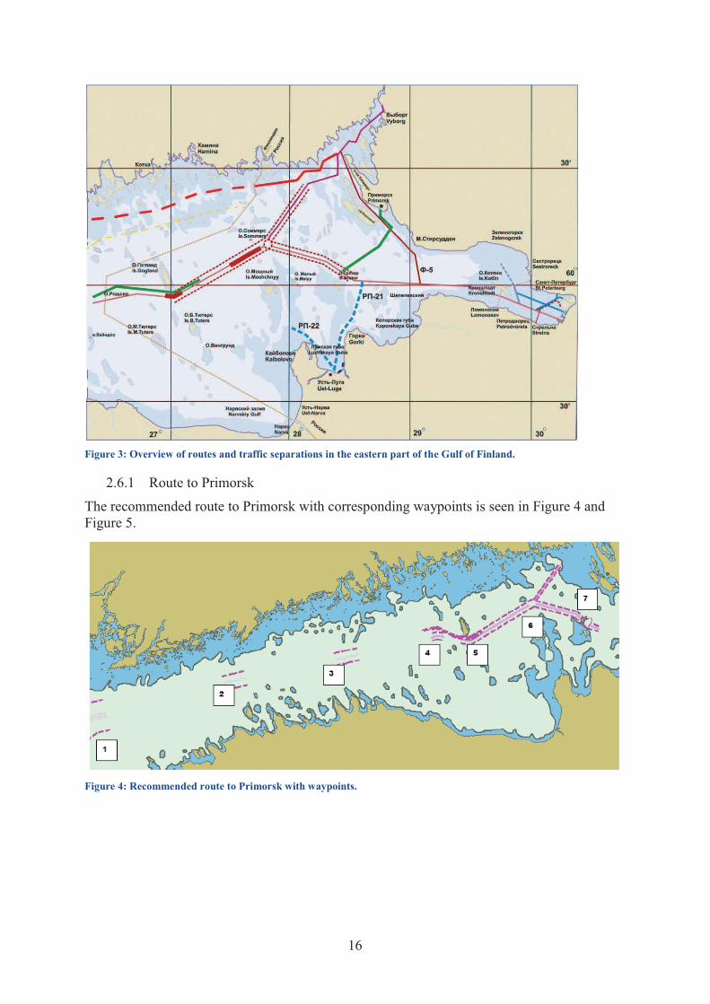
Figure 3: Overview of routes and traffic separations in the eastern part of the Gulf of Finland.

2.6.1 Route to Primorsk

The recommended route to Primorsk with corresponding waypoints is seen in Figure 4 and

Figure 5.

Figure 4: Recommended route to Primorsk with waypoints.

17

Figure 5: Zoom of the eastern GoF with recommended route and corresponding waypoints to Primorsk.

The position and distance between the waypoints are presented in Table 2.

Table 2: Position and distance between waypoints shown in Figure 4 and Figure 5.

Point Distance Comments N E N E (nm)

1 59 32.00 022 43.40 59.5333 22.7233 2 59 45.00 024 21.80 59.7500 24.3633 51.41 3 59 53.00 025 38.40 59.8833 25.6400 39.34 4 60 00.00 026 40.87 60.0000 26.6812 32.07 5 59 58.80 027 01.90 59.9800 27.0317 10.59 HOG 6 60 11.40 027 46.70 60.1900 27.7783 25.65 7 60 07.59 028 16.50 60.1265 28.2750 15.31 8 60 05.20 028 21.90 60.0867 28.3650 3.60 SES 9 60 10.50 028 42.70 60.1750 28.7117 11.64 10 60 15.20 028 48.40 60.2533 28.8067 5.49 11 60 19.70 028 42.10 60.3283 28.7017 5.48 PRI

Total distance HOG - PRI 67.2 nm Total distance GoF 200.6 nm

Position Position

18

3. Database

This chapter explains what data that has been used, how and why the data has been recorded

in the database.

3.1 Raw material

In this chapter the material used to create the database is presented.

3.1.1 Adveto Aecdis-2000 ver. 2009-09-01

Aecdis-2000 is a product from Adveto AB. It is a system for presentation of nautical charts

according to the Electronic Chart Display and Information System (ECDIS) standard. In this

study it has been used to replay the AIS tracks of the desired oil tankers and the assisting

icebreakers.

3.1.2 Automatic Identification System data

Automatic Identification System (AIS) data is available for a number of winters amongst

them 2006. The winter navigation research board has gathered information about the transits

of larger oil tankers to the ports in the eastern GoF. Also there is data from the icebreakers

that have been assisting in the area. The data covers the roundtrip transits from ice edge to

port. The data has been recorded in ADVETO AECDIS-2000v3 and is saved on a day to day

basis in Access (.mdb) format.

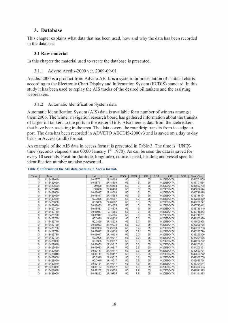
An example of the AIS data in access format is presented in Table 3. The time is “UNIX-

time”(seconds elapsed since 00:00 January 1st 1970). As can be seen the data is saved for

every 10 seconds. Position (latitude, longitude), course, speed, heading and vessel specific

identification number are also presented.

Table 3: Information the AIS data contains in Access format.

Type Time Lat Lon COG SOG HDG ROT AID POB CheckSum0 1113429610 60.08761 27.48393 55 6 55 0 25E8C47A 13437016600 1113429620 60.08761 27.48393 55 6 55 0 25E8C47A 13437016340 1113429630 60.088 27.48483 56 6 55 0 25E8C47A 13450277860 1113429640 60.088 27.48483 56 6 55 0 25E8C47A 13450276440 1113429650 60.08817 27.48583 55 6 55 0 25E8C47A 13437164780 1113429660 60.08817 27.48583 55 6 55 0 25E8C47A 13437164640 1113429670 60.0885 27.48667 55 5.9 55 0 25E8C47A 13492362590 1113429680 60.0885 27.48667 55 5.9 55 0 25E8C47A 13492362770 1113429690 60.08883 27.4875 55 6 55 0 25E8C47A 13437154420 1113429700 60.08883 27.4875 55 6 55 0 25E8C47A 13437153400 1113429710 60.08917 27.4885 55 6 55 0 25E8C47A 13437152430 1113429720 60.08917 27.4885 55 6 55 0 25E8C47A 13437152610 1113429730 60.0895 27.48933 55 6.1 55 0 25E8C47A 13435059260 1113429740 60.0895 27.48933 55 6.1 55 0 25E8C47A 13435059280 1113429750 60.08983 27.49033 55 6.2 55 0 25E8C47A 13432967680 1113429760 60.08983 27.49033 55 6.2 55 0 25E8C47A 13432967580 1113429770 60.09017 27.49133 55 6.2 55 0 25E8C47A 13432957760 1113429780 60.09017 27.49133 55 6.2 55 0 25E8C47A 13432958060 1113429790 60.0905 27.49217 55 6.3 55 0 25E8C47A 13442046760 1113429800 60.0905 27.49217 55 6.3 55 0 25E8C47A 13442047220 1113429810 60.09083 27.49317 55 6.3 55 0 25E8C47A 13442058110 1113429820 60.09083 27.49317 55 6.3 55 0 25E8C47A 13442058210 1113429830 60.09117 27.49417 55 6.5 55 0 25E8C47A 13426637540 1113429840 60.09117 27.49417 55 6.5 55 0 25E8C47A 13426637720 1113429850 60.0915 27.49517 55 6.9 55 0 25E8C47A 13429397500 1113429860 60.0915 27.49517 55 6.9 55 0 25E8C47A 13429397360 1113429870 60.09184 27.49617 55 7.3 55 0 25E8C47A 13463046410 1113429880 60.09184 27.49617 55 7.3 55 0 25E8C47A 13463046630 1113429890 60.09232 27.49735 55 7.7 55 0 25E8C47A 13443419230 1113429900 60.09232 27.49735 55 7.7 55 0 25E8C47A 1344341933

19

3.1.3 Ice charts

In this study Russian ice charts have been used. This manly because the chart contain

information about ice compression that the Swedish and Finnish ice charts are missing. The

charts are published by the Hydrometeorological Center of St.-Petersburg. The charts come as

GIF pictures. To be used in Adveto they have to be in a .BSB/.KAP format. This is a geo

referenced raster format often used for navigational purposes.

Figure 6 is an example of an ice chart of the GoF. See appendix A for translation from

Russian.

20

Figure 6: Example of Russian ice chart.

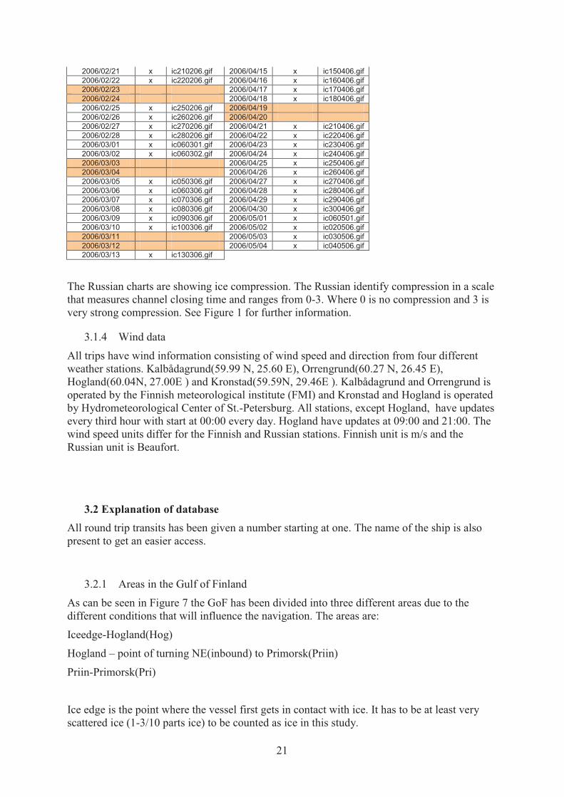
The ice charts available for 2006 can be seen in Table 4.

Table 4: Available Russian ice charts during the winter 2006. Marked dates are unavailable.

2006/01/20 x ic200106.gif 2006/03/14 x ic140306.gif 2006/01/21 x ic210106.gif 2006/03/15 x ic060315.gif 2006/01/22 x ic220106.gif 2006/03/16 x ic060316.gif 2006/01/23 x ic230106.bmp 2006/03/17 x ic170306.gif 2006/01/24 x ic240106.gif 2006/03/18 x ic180306.gif 2006/01/25 x ic250106.gif 2006/03/19 2006/01/26 x ic260106.gif 2006/03/20 x ic200306.gif 2006/01/27 x ic270106.gif 2006/03/21 x ic210306.gif 2006/01/28 x ic280106.gif 2006/03/22 x ic220306.gif 2006/01/29 x ic290106.gif 2006/03/23 x ic230306.gif 2006/01/30 x ic300106.gif 2006/03/24 x ic240306.gif 2006/01/31 x ic310106.gif 2006/03/25 x ic250306.gif 2006/02/01 x ic060201.gif 2006/03/26 2006/02/02 x ic060202.gif 2006/03/27 2006/02/03 x ic030206.gif 2006/03/28 x ic280306.gif 2006/02/04 2006/03/29 x ic290306.gif 2006/02/05 x ic050206.gif 2006/03/30 x ic300306.gif 2006/02/06 x ic060206.gif 2006/03/31 x ic310306.gif 2006/02/07 x ic070206.gif 2006/04/01 x ic060401.gif 2006/02/08 x ic080206.gif 2006/04/02 x ic060204.gif 2006/02/09 x ic090206.gif 2006/04/03 x ic030406.gif 2006/02/10 x ic100206.gif 2006/04/04 x ic040406.gif 2006/02/11 2006/04/05 x ic050406.gif 2006/02/12 x ic120206.gif 2006/04/06 x ic060406.gif 2006/02/13 x ic130206.gif 2006/04/07 x ic070406.gif 2006/02/14 x ic140206.gif 2006/04/08 x ic080406.gif 2006/02/15 x ic150206.gif 2006/04/09 2006/02/16 x ic160206.gif 2006/04/10 x ic100406.gif 2006/02/17 x ic170206.gif 2006/04/11 x ic110406.gif 2006/02/18 x ic180206.gif 2006/04/12 x ic120406.gif 2006/02/19 x ic190206.gif 2006/04/13 x ic130406.gif 2006/02/20 x ic200206.gif 2006/04/14 x ic140406.gif

21

2006/02/21 x ic210206.gif 2006/04/15 x ic150406.gif 2006/02/22 x ic220206.gif 2006/04/16 x ic160406.gif 2006/02/23 2006/04/17 x ic170406.gif 2006/02/24 2006/04/18 x ic180406.gif 2006/02/25 x ic250206.gif 2006/04/19 2006/02/26 x ic260206.gif 2006/04/20 2006/02/27 x ic270206.gif 2006/04/21 x ic210406.gif 2006/02/28 x ic280206.gif 2006/04/22 x ic220406.gif 2006/03/01 x ic060301.gif 2006/04/23 x ic230406.gif 2006/03/02 x ic060302.gif 2006/04/24 x ic240406.gif 2006/03/03 2006/04/25 x ic250406.gif 2006/03/04 2006/04/26 x ic260406.gif 2006/03/05 x ic050306.gif 2006/04/27 x ic270406.gif 2006/03/06 x ic060306.gif 2006/04/28 x ic280406.gif 2006/03/07 x ic070306.gif 2006/04/29 x ic290406.gif 2006/03/08 x ic080306.gif 2006/04/30 x ic300406.gif 2006/03/09 x ic090306.gif 2006/05/01 x ic060501.gif 2006/03/10 x ic100306.gif 2006/05/02 x ic020506.gif 2006/03/11 2006/05/03 x ic030506.gif 2006/03/12 2006/05/04 x ic040506.gif 2006/03/13 x ic130306.gif

The Russian charts are showing ice compression. The Russian identify compression in a scale

that measures channel closing time and ranges from 0-3. Where 0 is no compression and 3 is

very strong compression. See Figure 1 for further information.

3.1.4 Wind data

All trips have wind information consisting of wind speed and direction from four different

weather stations. Kalbådagrund(59.99 N, 25.60 E), Orrengrund(60.27 N, 26.45 E),

Hogland(60.04N, 27.00E ) and Kronstad(59.59N, 29.46E ). Kalbådagrund and Orrengrund is

operated by the Finnish meteorological institute (FMI) and Kronstad and Hogland is operated

by Hydrometeorological Center of St.-Petersburg. All stations, except Hogland, have updates

every third hour with start at 00:00 every day. Hogland have updates at 09:00 and 21:00. The

wind speed units differ for the Finnish and Russian stations. Finnish unit is m/s and the

Russian unit is Beaufort.

3.2 Explanation of database

All round trip transits has been given a number starting at one. The name of the ship is also

present to get an easier access.

3.2.1 Areas in the Gulf of Finland

As can be seen in Figure 7 the GoF has been divided into three different areas due to the

different conditions that will influence the navigation. The areas are:

Iceedge-Hogland(Hog)

Hogland – point of turning NE(inbound) to Primorsk(Priin)

Priin-Primorsk(Pri)

Ice edge is the point where the vessel first gets in contact with ice. It has to be at least very

scattered ice (1-3/10 parts ice) to be counted as ice in this study.

22

Hogland is an island and the point that is counted for the areas are the longitude (27° 00’E) of

the southernmost tip. Priin is the point where the vessels turns NE inbound for Primorsk.

Approximate position (60° 06’ N, 28° 23’ E)

Primorsk is the port of Primorsk.

Figure 7: The areas chosen because of the different navigational conditions.

All particulars are recorded for the different areas. There is also a forth area or state and that is

time at terminal. For terminal time there are no particulars except the time of arrival,

departure and total duration.

3.2.2 Ice classes

The ice class according to the Finnish Swedish rules is recorded.

3.2.3 Ice particulars

The following particulars are available for the ice conditions.

Ice thickness

The thickness in the area is recorded as a span in cm.

Type of ice

Recorded as x/10 parts of ice. In the case of land fast ice it is recorded as land fast and not by

parts. If there is different types of ice it is recorded as an example 2→ 10 meaning it starts as a 2/10 part ice and later on it is 10/10. In the Russian charts the different parts are 9-10/10, 7-

8/10. 4-6/10, 1-3/10. They are recorded as 10, 8, 5, 2 respectively.

Compression

23

The compression in the area as stated in the ice charts. This is the Russian scale for

compression were 0 is no compression and 3 is maximum compression. When there is

differences in the area the different compressions are separated with a comma. This is also

the case if the ice compression is 1-2 or 2-3. If the ice conditions were the vessel has been

sailing don’t approve of compression, land fast ice or not enough ice concentration, the

compression is recorded as zero comma one.

Hummocking

If hummocking is present it is stated as 1 for true and 0 for false. Hummocking meaning there

are ridges present in the ice cover.

3.2.4 Icebreaker

The icebreaker column is zero for no icebreaker assistance and if there has been assistance

parts of the transit in that area it is stated by the name of the icebreaker. Observe that it does

not mean that there has been assistance the entire time.

3.2.5 Transit particulars

Stop and waiting is decided to be from the time that the speeds gets below 1 knot. The

icebreaker and self transit times is therefore at velocities higher that 1 knot.

Icebreaker time

Transit time with an assisting icebreaker.

Self transit

Time under way without icebreaker assistance.

Stop

A stop is caused by the ice conditions. Not an ordered stop by the icebreaker. A limit of two

hours is set to separate waiting time and stop time. One stop can therefore not be longer than

two hours because then it is assumed to be a waiting period. Stops are thought to be an

indicator for how tough the transit is.

There is one column with number of stops and one with the total stop time for all the stops in

the area.

Waiting

Waiting time is defined as a longer period of time waiting for icebreaker assistance, waiting

for clearance at the oil terminal or waiting cause the traffic situation orders a wait. This is

usually a longer time span and if it isn't obvious that it is waiting time, such as waiting outside

the terminal or getting picked up after a shorter waiting with self transit before that, the

minimum time for recording as waiting is two hours.

There is one column with how many different waiting periods and one column with the total waiting time in the area.

Activity order

The column with activity order is describing in what order the different activities was carried

out. Every new activity is presented as a number, see below for explanation, and a time when

that activity starts in parenthesis. If it is needed the date is also included in the parenthesis.

The number code for activities.

24

1 = self transit

2 = icebreaker assistance

3 = stop

4 = wait

5 = waiting for terminal

6 = terminal

Activity comment

Comments about difference in the route, if there has been multiple vessels assisted by the

same icebreaker, drift speed and direction when lying still and other things that deviate from

the usual procedure.

3.2.6 Average speed

The speed is an average in that particular area during transit and do not include stop and

waiting time. Both self transit and time with icebreaker assistance are included.

3.2.7 Distance

This is an approximate distance travelled in that area extracted from the product of average

speed and the sum of icebreaker time and self transit time.

3.2.8 Ice edge longitude

The longitude of the ice edge on the same day as the vessel crosses it. Not were the vessel

crosses but the actual extent of the ice edge.

3.2.9 Weather

All four stations have the current weather with wind speed and direction recorded. Wind

speed is in m/s for Kalbådagrund and Orrengrund and in Beaufort for Hogland and Kronstadt.

The direction is in degrees for all stations.

3.2.10 Extra material

Every round trip transit is recorded separately before inserted in the database. Some additional

information is stored in those files that are not included in the database. The track of the

current tanker is plotted on the ice chart. Inbound and outbound transits are plotted separately.

With this information it is easy to get a quick overview of the trip and the ice conditions

encountered. Furthermore the activity is recorded on a separate sheet to make it more

accessible and make it easier to plot. Time axis plots of the activities are made to get a

overview of the traffic pattern on that trip.

3.3 Procedure

To convert the ice charts from a standard .gif picture a library called libbsb-0.0.7[11], run in Windows on a Unix like shell MSYS, has been used. MSYS is a component in

MinGW(Minimalist GNU for Windows) and are both free ware.

An oil tanker transit was picked, on the basis that there have to be different ice classes and

there has to be different ice compression in the database, and its tracks were compared with

the icebreakers to see if there had been any assistance during the transit.

25

In Adveto Aecdis-2000 the AIS tracks from the current tanker and possible an assisting

icebreaker were loaded and replayed at high speed. The information about stop, icebreaker

assistance, self transit times, what time they enter a new area etc was recorded.

The AIS data was copied from Access to Excel to evaluate the average speed. To make the

AIS data easier to work with every whole minute, instead of every 10 seconds, was extracted.

A macro called Sortera_hela_minuter.xls was used for that. The conversion to make the Unix

time workable, that is convert to regular date and time, a macro called Funktion_DatumU.xls

was used.

The velocities for the different areas were calculated and recorded. The average speed is area

specific and all the time with velocities over one knot were accounted for. The distance

travelled followed after the average speed was calculated.

Finally the weather was recorded. The average of wind speed and direction during the area

transit was calculated.

26

4. Analysis

4.1 Traffic pattern

This part is connected to the last problem formulation. What are the expected average values

for a transit to Primorsk? In other words the traffic pattern is to be investigated by average

numbers. This part is especially interesting when planning a route. With the expected values

on transit times, number of stops etc. the vessels in a shipping company can be used more

efficient.

The following transit particulars have been focused on. All parts are divided into inbound and

outbound cause there might be a difference between them.

Transit time. Here the transit time outbound, inbound and round trip transit are the main

focus.

Waiting time. The average waiting time and how many times during a transit that waiting

occurred.

Icebreaker time. Average time with assistance of a icebreaker.

Stop time. How many times the tanker came to a stop during a transit.

Average speed. The average speed of all tankers in all kinds of conditions. Because of the

different navigational conditions in the different areas the speed parameter will be

investigated within the different areas and not just inbound and outbound. The different areas

will be compared depending if it is inbound or outbound.

Time at terminal. How much time that is spent at terminal.

To take the distance travelled into account some percentage values has been studied. The

percentage of icebreaker time compared to the total transit time has been analysed. The transit

time percentage is not that interesting because speed is a pointer that does take distance

travelled into account and is connected to the transit time.

4.2 Ice class

To see if there is a trend between ice classes, i.e. see if the higher classes perform better

according to the Swedish Finnish ice class, is another purpose of this study.

Measurable variables that indicate better performance are velocity, waiting time and time with

icebreaker assistance and are hence analysed.

Different ice classes have been recorded in the database. AFRAMAX tankers with ice class

1AS, 1A, 1B and 1C. These are given a number, 1 for 1C, 2 for 1B, 3 for 1A and 4 for 1AS.

That makes them easier to work with.

Linear regression is used to see if there is a trend. The ice class is compared with speed,

waiting time and icebreaker time percentage separately. The percentage on icebreaker time is

used because it is believed that it gives a better picture when the distance travelled is

included.

4.3 Wind and ice compression correlation

To evaluate the accuracy on the compression on the ice charts and/or the wind data the

correlation between the two has been investigated. It is believed that stronger winds result in

27

more severe ice compression given the same wind direction. In this analysis the force of the

wind is the only wind parameter present.

The wind data from the Hogland station is believed to be inaccurate time wise since it is only

updated every 12th

hour. Therefore that particular station is not included in this part of the

study.

As stated in chapter 2.2 the ice compression is sometimes recorded as 0,1 because of different

ice conditions in the particular area. Since this part has the objective of finding the correlation

between compression and wind force the compression has always been thought of as one in

those cases. If it is thought of as zero instead there might be some values that would point in

the wrong direction.

The different areas included are iceedge-HOG and HOG-Priin. The area Priin-Pri is

considered to unsure because there is mainly landfast ice there and thus the compression is

recorded as zero in the database. That makes it very hard to find a reliable correlation there.

The correlation has been studied between the compression in the area of iceedge-HOG and

the wind force from Kalbådagrund and Orrengrund. In this area the wind force from

Kronstadt are considered inaccurate since Kronstadt is too far away.

The ice compression data from the area HOG-Priin has been correlated with wind data from

all three weather stations.

The data is gathered in a scatter plot divided into areas and weather station. In the plots you

are able to see if there is a notable difference in wind speed depending on the compression.

4.4 Ice compression and transit particulars

4.4.1 Speed

At stronger compression the channel behind the vessel or behind assisting icebreaker starts to

close at a faster rate. The forces generated on the investigate vessels hull gets bigger and it is

harder to proceed. An assumption is that the velocity of that ship should be affected in a

negative way.

The impact of compression on speed has been studied.

As in the previous chapter the area Priin-PRI is not considered relevant due to the land fast ice

there and is hence not included in the calculations. The two other areas, ice edge-Hog and

Hog-Priin, are included. The dependency is analysed in the different areas separately. Inbound

or outbound divided to separate areas and the total regardless of direction are studied.

In the area ice edge-HOG the compression is sometimes recorded as 0,1 due to different ice

conditions. This is solved by doing the calculations for both states. One were 0,1 is regarded

as 1 and the other were it is regarded as 0.

The average values of speed from the different areas and states of compression are calculated.

Scatter plots of all value, areas and states of compressions are made to find a possible speed

compression dependency.

4.4.2 Waiting time

More compression is believed to get the result that vessels encounter more resistance and

there is a possibility that the vessel gets stuck. The vessel might need icebreaker assistance, or

the traffic situation might not be considered safe enough because of the compression and the

28

vessel gets ordered to wait. The waiting periods is believed to be more frequent and longer.

This part of the thesis is analyzing what influence ice compression has on the waiting time.

The analysis is divided into inbound transit and outbound transit.

The waiting time is added from the three different areas on a single transit. The compression

for the same singe transit is simplified to the maximum of the three areas. Here a difference in

ice compression in a certain area is considered as the larger number.

4.4.3 Icebreaker time

As with the waiting time the time with icebreaker is believed to be correlated to ice

compression. The increasing resistance the vessels encounter at ice compression might be too

much and icebreaker assistance is a must. In this part we see if there is a noticeable difference

in time with icebreaker assistance depending on the degree of compression.

Two different approaches have been used. The first approach is comparing time with assisting

icebreaker and compression. The second one using parts of time with assisting icebreaker per

total transit time under way (time under way including self transit and icebreaker assistance)

comparing this with the ice compression.

Inbound and outbound transits has been studied separately, from ice edge to Primorsk and the

other way around respectively.

The data from the tanker Tempera has not been included since it is build to navigate

independently and with the relatively low degree of compression the year of 2006 it should

not be a problem for her to navigate independently

The compression used is the highest number of the three areas included in the current inbound

or outbound transit.

4.5 Technical estimate of ice resistance originating from ice compression

In chapter 2.3.5 the ice resistance in the Lindqvist formula (6) was discussed. This part will

explain how an estimate of the ice resistance contributed from the ice compression has been

evaluated by means of that formula. The reason for choosing Lindqvist formula is that it gives

the ice resistance as a function of velocity. The equation is initially intended for smaller

vessels in level ice. The larger vessels with different hull shape might not respond in the same

way as the intended vessels but no problems are mentioned about using it on larger vessels

such as AFRAMAX tankers. In this calculation it is ignored that the tankers sometimes sails

in brash ice and it is assumed that they are in level ice.

The input variable speed is imported from the results that shall be generated as stated in

chapter 4.4.1. The speed at compression 0, 1 and 1-2 is extracted there and will be used to see

what extra resistance arise at compression 1 and 1-2.

To make sure the ice conditions are similar the area Hog-Priin are the only area used. The thickness is basically the same the entire observation period and the parts of ice are always 9-

10/10 and land fast ice rarely exists.

29

5. Results

There are 41 roundtrip transits recorded in the database.

5.1 Traffic pattern

5.1.1 Icebreaker assistance

It has been observed that icebreaker assistance usually takes place east of Hogland, both

inbound and outbound. There are only three icebreakers that have been assisting the observed

AFRAMAX oil tankers sailing on Primorsk in the winter of 2006. Those are the big Russian

icebreakers Kapitan Sorokin, Admiral Makarov and Ermak.

The time with an assisting icebreaker and the percentage of time under way with icebreaker

assistance can be seen in Table 5. The values presented are averages from all transits

observed. Both time and percentage time shows that the tankers get more assistance on the

outbound transit.

On an outbound transit the tankers are assisted almost half of the time under way. That means

half of the way to the ice edge on average. This takes about eight hours outbound. Inbound

the tankers gets a bit less time with icebreaker assistance, about six hours which accounts for

36% of the time under way.

Table 5: Average icebreaker assistance as percent of time under way and time with assisting icebreaker with corresponding standard deviation divided into inbound and outbound transit.

Percent of ib. ass. of total

time under way

Stdev. Ib. ass. %

Time with Ib.

Ass.

Stdev. Ib. ass.

Inbound 36

23 06:11

04:01

Outbound 47

17 08:18

03:09

5.1.2 Waiting and stop

During a roundtrip transit the average number of times a tanker had to wait was almost three

times (as can be seen in Table 6). Inbound the number of waiting periods was just over two

and outbound just short of one. Many times during an outbound transit the tankers have to

wait for the icebreaker just outside the terminal. A similar behaviour has been observed on an

inbound transit. The tankers frequently have to wait to get a docking place at the oil terminal.

The inbound tankers might also have to wait if they are getting icebreaker assistance. These

observations fit in pretty good with the average number of waiting periods calculated.

As for waiting time it can be seen in Table 7. On average the roundtrip waiting time is just

short of 37 hours. Nearly all the waiting is done on the inbound journey, accounting for more

than 33 hours of the total 37. Outbound the tankers only have to wait for just over three hours.

Table 6: The number of stop and waiting periods with standard deviation on an inbound, outbound and roundtrip transit respectively.

# wait Stdev. # wait # stop Stdev. # stop

Inbound 2.05 1.05 1.07 0.91

Outbound 0.88 0.84 1.20 1.38

Roundtrip 2.93 1.17 2.27 1.64

30

Stops occur a bit more than twice per roundtrip transit and each lasts for about 30 minutes.

The stops are divided pretty evenly between inbound and outbound transits. Just slightly more

stops in average on the outbound transits.

5.1.3 The Mean transit

In this chapter the results concerning consumed time during a transit is presented. In Table 7

all values are included. The different states that consume time, defined in chapter 3.2.5, are in

the left column. The time spent in each state is presented in three different areas, inbound,

outbound and roundtrip transit. To make the roundtrip transit complete the time at terminal is

added to its total time.

Table 7: Time on transit divided into activities.

Inbound Outbound Roundtrip

Self 10:51:00 9:56:00 20:47:00

Ib. Ass 6:11:00 8:18:00 14:30:00

Wait 33:45:00 3:07:00 36:52:00

Stop 0:32:00 0:26:00 0:58:00

∑ 51:19:00 21:47:00 73:07:00

Terminal

25:16:00

∑ 98:23:00

Observing Table 7 and Figure 8 it can be seen that the tanker spends more than twice as

much time inbound than outbound. The time at terminal is slightly longer than the outbound

transit and just short of half the inbound time. An inbound transit stands for more than half of

the roundtrip transit time. The outbound transit and time at terminal accounts for

approximately a quarter each.

Figure 8: Average time spent on inbound transit, outbound transit, at terminal and the sum of the three as roundtrip transit.

0:00:00

12:00:00

24:00:00

36:00:00

48:00:00

60:00:00

72:00:00

84:00:00

96:00:00

108:00:00

inbound outbound terminal roundtrip

Tim

e(h

h:m

m:s

s)

Total time spent during transit

31

In Figure 9 some values from Table 7 have been highlighted. The waiting time is the largest

contributor on a roundtrip and is even more dominant on inbound transits. Time under way is

slightly less inbound. The biggest difference except for waiting time is time with icebreaker

assistance that is less inbound. The time at stop is almost negligible as it only stands for about

1 % of the total roundtrip time.

Figure 9: Average time spent on different activities on inbound, outbound and roundtrip transits.

5.1.4 Average speed

The result of the speed analysis of the observed tankers is presented in this chapter. The main

focus was to see if there was a speed difference between inbound and outbound transit. Due to

different navigational conditions in the GoF, which was believed to influence the speed, both

analyzes was carried out on the three areas predetermined in chapter 3.2.1.

Figure 10 shows that the speed is higher inbound on all three areas. Most notable between

HOG-Priin were the difference is 0.9 knots.

0:00:00

6:00:00

12:00:00

18:00:00

24:00:00

30:00:00

36:00:00

42:00:00

inbound outbound roundtrip

Tim

e(h

h:m

m:s

s)

Average transit to Primorsk

self

ib. Ass

wait

stop

32

Figure 10: Average speed inbound and outbound in the three determined areas.

5.2 Ice classes

The different ice classes, defined by the Finnish Swedish ice class, are classed for different

degrees of winter navigation conditions. They all have different hull strength, propulsion

power etc to cope with the conditions they are classed for. The results from the ice conditions

in the database show that the thickness does not add up to the thickness set for classing the

different ice classes. Occasionally during the winter there has been ice thickness up to 0.65 m.

That is just above the thickness defined for ice class 1C that is the lowest class observed.

5.2.1 Speed

The ice class rules stipulate a minimum speed of five knots in a given ice thickness for the

different classes. The same conditions and thickness with some random deviation has applied

during these observations and the speed of the vessels has been investigated divided on ice

class. In Table 2Table 8 speed in the two different areas has been compared to the ice classes.

The speed is average from all tankers divided into ice class and area. The areas include both

inbound and outbound transits.

Table 8. Average speed for different ice classes in different areas.

Area /

Ice class

Ice edge ↔

Hog

Hog ↔

Priin

1AS 14,04 10,87

1A 12,47 10,95

1B 11,94 9,86

1C 12,56 11,10

In Figure 11 the data is visualised. On the x-axis are the ice classes. The numbers represents

ice classes as 1 is class 1C, 2 class 1B, 3 is 1A and 4 is class 1AS. As can be seen there is a

rising trend in the area ice edge-Hog. In the area Hog-Priin there is no visible trend. In both

areas ice class 1C has higher speed than ice classes 1B and 1A. Between Hog and Priin ice

class 1C has even higher speed than class 1AS. Class 1B has the lowest speed in both areas.

0,0

2,0

4,0

6,0

8,0

10,0

12,0

14,0

Iceedge-HOG HOG-Priin Priin-PRI

Sp

eed

(kn

) Speed difference inbound and outbound

inbound

outbound

33

Figure 11: Average speed in knots and ice classes compared on inbound and outbound transit. Ice classes on x-axis as numbers (1=1C, 2=1B, 3=1A, 4=1AS).

The distributions of the average speed values compared to ice classes are shown in Figure 23

and Figure 24 in appendix D.

5.2.2 Icebreaker

In chapter 2.1.1 it is explained that different ice classes are classed for more or less time with

icebreaker. The result from the analysis on icebreaker time compared to ice classes is

presented in Table 9 and Figure 12.

Table 9: Average parts of transit under way with icebreaker assistance compared with ice class on inbound and outbound transit respectively.

Ice class /Area INBOUND OUTBOUND

1C 0,28 0,56

1B 0,32 0,50

1A 0,49 0,44

1AS 0,10 0,25

In Figure 12 the ice classes have been given a number explained in the previous chapter. The

icebreaker time is presented as the fraction of icebreaker assistance compared to total time

under way. There is a visible trend on outbound transit with a sinking icebreaker fraction for

stronger ice class. Inbound class 1A has by far the largest fraction of icebreaker assistance

followed by class 1B and 1C and finally 1AS even further down. Both inbound and outbound

ice class 1AS has the lowest fraction of icebreaker assistance.

9

10

11

12

13

14

15

0 1 2 3 4 5

Sp

eed

(kn

)

Ice class

Hog-Priin

Iceedge-Hog

34

Figure 12: Average parts of transit under way with icebreaker assistance compared to ice classes on inbound and outbound transit. Ice classes on x-axis as numbers(1=1C, 2=1B, 3=1A, 4=1AS).

5.2.3 Waiting time

In Figure 13 the ice classes is matched with the waiting time and compared. It can be seen

that inbound transit has a negative trend with decreasing waiting time with rising ice class.

Outbound the waiting time is highest for ice class 1A and lowest for 1AS but the gap is less

than 3 hours. The outbound waiting time is small compared to inbound waiting time and

consequently the roundtrip waiting time follows the same trend as the inbound transit.

Figure 13: Average waiting time for different ice classes. Ice classes on x-axis as numbers(1=1C, 2=1B, 3=1A, 4=1AS).

0

0,1

0,2

0,3

0,4

0,5

0,6

0 1 2 3 4 5

Pa

rt o

f tr

an

sit

wit

h i

ceb

rea

ker

Ice class

INBOUND

OUTBOUND

0,00

10,00

20,00

30,00

40,00

50,00

60,00

0 1 2 3 4 5

Wa

tin

g t

ime(

h)

Ice class

Inbound

Outbound

Roundtrip

35

5.3 Ice compression

5.3.1 Wind and ice compression correlation

The available wind and compression data has been studied for correlation. Ice compression

data originates from Russian ice charts and wind data from both Russian and Finnish weather

stations. In the area ice edge-Hog the ice compression has been studied towards wind speed

from Finnish stations Kalbådagrund and Orrengrud. The area between Hog-Priin has had the

same analysis with the addition of wind speed from Russian station Kronstadt. In appendix C

there are plots of the data.

The correlation is weak through all tests. Pearson correlation coefficient has been calculated

and there is a very thin positive trend with rising compression as a result of rising wind speed.

Table 10: Pearson correlation coefficient on wind speed and ice compression in different areas.

Orrengrund Kålbådagrund Kronstadt

Area Ice edge - Hog Hog-Priin Ice edge - Hog Hog-Priin Hog-Priin

Pearson

correaltion 0.08 0.17 0.09 0.09 0.35

As can be seen in Table 10 all coefficients are positive but are all very weak. The only

exception is wind data from Kronstadt correlated with compression data from Hog-Priin. This

correlation is just weak not very weak.

5.3.2 Speed

In Table 11 the average speed is presented as a function of ice compression and area. Comp.

0,1→0 means that when different compression (0 and 1) has been recorded in the database the

value 0 has been used. Similarly if the single zero is a one then one has been used. All areas

include both the time inbound and outbound.

Table 11: Average speed in different ice compression and areas.

Comp./Area Ice edge↔Hog

comp. 0,1→1

Ice edge↔Hog

comp. 0,1→0 Hog↔Priin

0 12,52 12,55 10,93

1 12,59 12,51 10,29

1-2 11,64 11,64 10,14

The speed doesn’t vary much between the different interpretations of compression in the area

ice edge-Hog. This can be seen in Figure 14 were the points of those series overlap. The trend

in the area is slightly negative, less speed with higher compression. In the area Hog-Priin

there is a stronger negative trend were the speed decline with growing ice compression.

In appendix E in Figure 26, Figure 28 and Figure 29 the average values, used in these results,

are presented as the distribution turned out.

36

Figure 14: Average speed compared with ice compression in different areas.

5.3.3 Icebreaker time

The icebreaker time or rather the fraction of icebreaker time on total time under way has been

studied against ice compression and is presented in this chapter. Figure 15 shows the results

from the analysis. On the x-axis the ice compression is presented and the y-axis represents

how big the part with icebreaker assistance was compared to total time under way. The

different series in the figure are inbound and outbound transits. Outbound the linear trend line

is almost constant, inbound there is a negative trend with a top at 1 on the compression scale.

Figure 15: Average parts of transit under way with icebreaker assistance compared with ice compression.

9,00

9,50

10,00

10,50

11,00

11,50

12,00

12,50

13,00

0,00 0,50 1,00 1,50 2,00

Sp

eed

(kt)

Ice compression

Ice edge↔Hog

comp. 0,1→1

Ice edge↔Hog

comp. 0,1→0

Hog↔Priin

0,00

0,10

0,20

0,30

0,40

0,50

0,60

0 0,5 1 1,5 2

Pa

rt o

f tr

an

sit

wit

h i

ceb

rea

ker

Ice compression

inbound

outbound

37

5.3.4 Waiting time

In Figure 16 the waiting time compared to ice compression is presented. It can be seen that

inbound the waiting time increase with stronger compression whereas outbound it is the

opposite. The increase inbound is more notable than the decrease outbound. Inbound the

growth in waiting time increases from step to step but outbound the waiting times are the

same regardless of ice compression.

Figure 16: Average waiting time and ice compression

5.3.5 Ice resistance that stem from ice compression.

In this chapter the results from the estimation of the ice resistance that stem from ice

compression are presented. Lindqvists equation (6) has been used with different velocities

depending on compression, taken from chapter 5.3.2, in the area Hog-Priin. The ice thickness

was around 40 cm in this area the entire observation period and this thickness has been used.

Generic values for an AFRAMAX tanker have been used. For the entire list of input variables

see Table 15 in appendix F.

In Table 12 the results of the calculations are presented. The ice compression, ice resistance at

average speed, delta ice resistance, ice resistance at average speed minus one standard

deviation and ice resistance at average speed plus one standard deviation in columns from left

to right. The delta resistance is the estimate of ice resistance that stem from ice compression

and is extracted from subtraction of resistance at 1, 1-2 ice compression from ice compression

at zero respectively. When there is 1 in compression the extra ice resistance is 183 kN on a

generic AFRAMAX tanker. The same value for 1-2 in compression is 226 kN. The standard

deviations from the average velocities are used to show the variation the scattered speed

values give rise to. The two right columns present ice resistance from Lindqvist’s formula

when one standard deviation has been subtracted and added to the average speeds.

0:00:00

6:00:00

12:00:00

18:00:00

24:00:00

30:00:00

36:00:00

42:00:00

48:00:00

0 0,5 1 1,5 2

Tim

e(h

h:m

m:s

s)

Ice compression

inbound

outbound

38

Table 12: Ice resistance that stem from ice compression extracted with Lindqvist(6).

Ice compression Ri (kPa) ∆Ri from 0 comp.(kPa) Ri (at speed -stdv) Ri (at speed +stdv)

0 3926 --- 3502 4350

1 3742 183 3370 4147

1-2 3699 226 3130 4269

39

6. Discussion

6.1 Database

The foundation for all studies in this thesis is the raw material. The ice charts used in this

study are available on a day to day basis. The AIS data used are updated once every minute.

The change in ice might not be as fast as the vessels transit times but there have been some

big changes between days during 2006. This can result in recorded values derived from the

ice charts are somewhat inaccurate.

The source of all transit information is the AIS data. Wait, stop, self transit etc has been

defined to best match the way the information is gathered. When the transit particulars are

collected the AIS data is played back in Adveto. What is seen is basically a dot moving in a

direction with a certain speed. There is no live onboard data and what really happened is

impossible to say. The best example is for stop or wait. Stop should be when the ice

conditions made the vessel stop whereas wait is something ordered from the icebreakers or

harbour administration. It might be a stop even though the vessel is at a standstill for more

than two hours. The opposite that wait could be less than 2 hours might also occur.

The data is from the winter of 2006 that was a moderate ice winter and the results are valid

only for those conditions. The ice compression this winter was maximum 1-2. This is only

half of the Russian ice compression span. It should be mentioned that values on ice

compression are taken from the ice charts with 24 hours validity and therefore might a bit off

phase with wind data and transit data that are accurate on a couple of hours.

All correlations that have been studied are single parameter analysis. All correlations could

possibly be dependent on other variables than the one investigated. All other variables have

not been constant and can thus affect the results in a negative way. A possible single variable

correlation can be hidden by various other parameters that have not been taken into account in

the analysis.

Since the data have these properties there might be some uncertainties and when viewing the

results it should be kept in mind.

6.2 Traffic pattern

More than half of the time spent on a roundtrip transit to Primorsk is spent inbound. This is

mainly because of the long waiting periods in that direction. Almost 2/3 of the time inbound

is spent waiting. The waiting time inbound contributes for 1/3 of the roundtrip transit time.

The long waiting time inbound can be accredited the fact that there on average are two

waiting periods. In general there is one waiting period for icebreaker assistance or an ordered

wait and one waiting period for a terminal quay. Both these periods tend to be much longer

than the single waiting period outbound. What causes the traffic pattern to look like that is

hard to say. Naturally there would be more waiting inbound because the vessels have to fit

into a harbour schedule whereas outbound there is none. One thought is that the icebreakers

give priority to the outbound tankers over inbound ones because the capacity does not allow

otherwise.

In an oil terminal a high priority is to keep a steady flow of oil out. By using a buffer of

tankers there will always be a tanker at quay ready to load up. Systematically using a buffer of

tankers can be the reason there is so much waiting time inbound. Some vessels are ordered to

wait outside the fairway, somewhere on the inbound transit, so that there is a buffer of ships

40

always ready to get to quay. The waiting can be of several days and at anchor. This system

was slowly implemented on the Russian oil ports 2006 but was more in use during 2007. [10]

The average speed is higher inbound than outbound. There might be a simple explanation to

the speed difference inbound and outbound. The fact that the tankers probably are fully

loaded outbound whereas inbound they are not. A ship often use the same power output

regardless of load. They either use maximum continuous revolution (MCR) or normal

continuous revolution (NCR). Using the same power output at ballast and fully loaded is the

probable explanation of the speed difference inbound and outbound.

6.3 Ice classes

There are three variables being compared to ice class to see if there are differences. Those are

waiting time, parts of transit with icebreaker assistance and speed. All variables have been

compared to ice class separately.

The speed of the different ice classes was analyzed for the areas ice edge – Hog and Hog –

Priin. Results show a trend with higher speed with higher ice class on both areas. Viewing

Figure 23 and Figure 24 in appendix D with all transit values present a wide spread are

observed. The correlation factors are very small for both areas. With the existing values there

is a positive trend but the lack of data makes it uncertain.

Waiting time compared to ice class gave a mixed result. The inbound waiting time correlated

very well with ice class while there on outbound waiting time was not any visible trend.

Inbound the results show that higher ice classes needed less waiting time. Inbound waiting

time being ten times more than outbound waiting time. The result of roundtrip transit was also

very well correlated with less waiting time with higher ice class. The not correlated outbound

waiting time might be a result of the general low waiting time outbound. Outbound the

tankers most often wait for icebreaker outside terminal for about three hours regardless of ice

class. If one random waiting period is longer than usual the effects on the average values are

more likely to be affected.

Part of icebreaker assistance on a transit results points towards a positive trend outbound and

a weak negative trend inbound. Positive means less parts of icebreaker assistance for higher

ice classes. Even though the positive trend is more solid than the negative one it is very hard

to draw any conclusions. As discussed later there are not many 1AS tankers recorded making

those values more vulnerable to chance. If the values from the 1AS tankers are disregarded

the trend inbound, and roundtrip for that matter, becomes strongly negative. Outbound the

trend is still positive. The final word with the available data is that there is no visible trend

between icebreaker assistance and ice class.

Apart from being too few transits in the database, that makes the results uncertain, there are not many transits recorded with vessels having ice class 1AS compared to the other ice

classes. This makes the results generated a bit uncertain because average values from 1AS

tankers are more easily affected by stray values. The trends become more uncertain with the

lack of transit data.

6.4 Ice compression and transit particulars

Unfortunately there has only been a maximum of 1-2 in compression during the winter of

2006. The scale continues up to 3 and 1-2 is only half of the max value. Not having the entire

scale represented makes it hard to decide how different parameters depend on the ice

compression. For an example it might look linear up to 1-2 and take a different turn after that

41

making it exponential or suchlike. All trends or correlation is therefore not representative for

the entire scale of compression but just up to 1-2.

A disclaimer is that the ice compression used is forecasted by the Hydro Meteorological

Center of St. Petersburg and the values presented on the charts might be put lower/higher than

they actually were because of a forecasted wind speed/direction available at the time.

The results in chapter 5.3.1 about wind speed and ice compression correlation are very weak.

The strongest Pearson correlation was 0.35 with wind force from Kronstadt and ice

compression from Hog-Priin. All analysis points towards rising ice compression with rising

wind speed but the correlation observed in the data studied is very weak and it is hard to draw

any conclusions. The direction of the wind is not regarded in the analysis and might be the

cause of the weak results. The wind direction might push the ice towards a not solid boundary

making the ice compression none existing. A multivariable analysis using both wind direction

and speed might give a better correlation.

The velocity of the tankers was compared with ice compression. The results show a moderate

decline in speed with higher compression in both areas investigated. Strongest result in terms

of speed decline and correlation is in the area Hog-Priin. But due to little data both results are

weak. Studying Figure 27 thru Figure 29 the scattered values are presented. As can be seen

the area Ice edge – Hog does not include more than four points with compression 1-2. This

makes the average values uncertain. The two different interpretations of compression in that

same area do not give rise to any bigger differences in the results. Probably because not too

many values was involved in the conversion. In the area Hog-Priin there are more occasions

when ice compression 1-2 occurs. There is a big spread of the values in the respective areas.

To conclude the average values presents a fairly good picture but the original values are very

scattered and the correlation is very weak in most cases. The speed is most likely not only

affected by the ice compression but also from other variables. Ice thickness, ridges, icebreaker

assistance and experience of the crew are some of them. The results only give a correlation

with ice compression.

Parts of icebreaker assistance on total time in transit is a way to measure time with icebreaker

assistance and in a sense taking distance travelled into account. Compared with ice

compression there was different results inbound and outbound. Inbound there was a linear

trend pointing towards less parts of icebreaker assistance with higher compression. On the

other hand the values at 1 in compression had the highest fraction of icebreaker assistance

inbound. The linear trend is not that strong. Outbound there was no difference in parts of

icebreaker assistance between the different compressions. Both trends are uncertain and it is

hard to draw any conclusions with the low correlations. The results points towards that there is no correlation between icebreaker assistance and ice compression.

Inbound there is an increase in waiting time with increasing compression. Outbound basically

the same waiting time is observed for 0 and 1 in compression and a dip at compression 1-2 is

noted. For the roundtrip transit the waiting time is also rising with more compression due to

the fact that most waiting time is on the inbound transit and therefore overwhelms the

outbound waiting time. Observing the average values a clear trend is seen with more waiting

time with higher compression. Looking at all values they are scattered and the correlation

makes it hard to draw any conclusion looking at all values. More data is needed.

42

6.5 Technical estimate of ice resistance

The values estimated in chapter 5.3.5 are guide values for how much extra resistance an

AFRAMAX tanker will encounter at compressions up to 1-2. The sources of errors are many

and the results have to be reviewed with carefulness.

It is assumed that the tankers use the same output of power and hence the speed decreases

when there is more ice resistance due to compression. If compression occurs the vessels

probably uses more propulsion power to avoid getting stuck. The values of extra ice

resistance calculated are therefore probably lower than the real encountered extra ice

resistance.

Other thing assumed that might affect the results are that the equation (6) is intended for

vessels smaller than AFRAMAX tankers and with different shape. Lindqvist never mentions

anything about applying the equations on other vessels but there could be a problem. Also the

equation is intended for level ice and in the area there is icebreaker assistance and hence not

level ice. When in brash ice the resistance encountered is lower than when in level ice,

assuming same ice conditions, and the speed will therefore be higher with same propulsion

power. Applying speed from brash ice makes the equation made for level ice uncertain.

Other input data such as generic values of the tankers, average ice conditions affect the

accuracy of the calculation. The speed input generated in this thesis is also a cause of

uncertainty. The values are scattered and the average is used. Observing the right most

columns in Table 12 that presents ice resistance at speed with one subtracted or added

standard deviation the variation is about 1000 kN for all compressions. Applying Lindqvist’s

formula on the separate transits might generate better results of the ice resistance.

To conclude the results are not exact but the ice resistance around 200 kN for both 1 and 1-2

in compression gives an order of magnitude.

43

7. Conclusion

The database created which is the foundation of the analysis consists of 41 roundtrip transits

to Primorsk during the winter of 2006 when the ice edge was west of Hogland.

Various analyses have been done that deals with ice compression. The period studied did not

include the entire spectra of ice compression. Maximum compression, on the Russian scale

that span from 0 to 3, was 1-2. The results presented are therefore only valid for the span 0 to

1-2 in compression. As for the analysis with ice classes and transit information there are too

few transits with 1AS tankers that make the results a bit uncertain for that particular ice class.

In general there could have been more data to make the results statistically stronger. Some

average values could show a correlation but the set of data behind the average values are

scattered and the correlations are very weak there and it is impossible to draw any

conclusions.

The purposes of this thesis have been answered to some extent. An average transit has been

presented. Interesting are the waiting time adding up to a third of the total roundtrip transit.

Almost all waiting occur on the inbound transit. Additionally the velocity differences with

higher velocity inbound than outbound is of interest. This is probably a result of tankers being

ballasted inbounds and with full load outbound combined with the tankers using the same

propulsion power regardless of load.

The analysis with ice class gave a dependency on waiting time whereas correlation towards

velocity and time with assisting icebreaker was very weak and therefore must be regarded as

independent from ice class.

The wind speed and ice compression correlation was weak but all results pointed towards that

stronger wind generated stronger compression. Furthermore there is a correlation between ice

compression and waiting time and ice compression and velocity. With stronger compression

the waiting times are longer and the velocity declines. Correlations were weak when ice

compression and icebreaker assistance was compared. The conclusion is that ice compression

does not affect time with icebreaker.

At ice compression 1 or 1-2 a generic AFRAMAX tanker encounter extra ice resistance. The

order of magnitude is 200 kN. The value for 1-2 in ice compression being slightly higher than

1. Simplifications in the calculation make it hard to present a more accurate value than a

magnitude.

44

8. Recommended further studies

To further develop this thesis more data in form of ship transits are needed. Many of the

results that have been extracted are weak because there is a lack of data. With more data the

statistical results would be stronger.

As for different studies there are some things that can be done. Multivariable analyse could

be made on many of the different analysis. Wind speed and ice compression analysis could be

extended to include wind direction. A similar analysis could be made for speed compared to

ice compression with more variables such as ice particulars and ice breaker assistance.

All studies including ice compression could be extended with compression from the entire

scale. The winter 2010 might be a god one where there has been cold weather generating

much ice and occasionally very strong winds. With the entire scale there could be some

interesting changes in the trends that have been studied. The behaviour might be different.

Results concerning traffic pattern might be used to compare with future years to see if

operations gets more efficient. For example the Russians are building new icebreakers that

intentionally will make operations flow better. Do they? Is there less waiting time or higher

speed? The system with a buffer of vessels to prevent a stop in oil loading was used more

during 2007 and further on. What are the effects of that? Is there for an example a trend with

more waiting because of that.

As mentioned in the discussion the estimate of ice resistance that stem from ice compression

could be made on the separate transits instead of the average values. In that way the more

specific ice thickness and speed would generate better values.

45

9. List of references

[1] Lindqvist, G(1989), A straightforward method for calculation of ice resistance of ships.

[2] Juva, M & Riska, K, Research report no. 53, On the power requirement in the Finnish

Swedish ice class rules.

[3] Riska, K; Wilhelmsson, M; Englund, K; Leiviskä, T, Research report no. 52, Performance

of merchant vessels in the Baltic.

[4] Eriksson, P; Haapala, J; Heiler, I; Leisti, H; Riska, K; Vainio, J, Research report no. 59,

Ships in compressive ice.

[5] Baltic icebreaker service, Baltic Sea Icebreaking Report 2005-2006,

http://portal.fma.fi/portal/pls/portal/!PORTAL.wwpob_page.show?_docname=2514132.PDF

[6] http://safewin.org/

[7] http://portal.fma.fi/sivu/www/baltice

[8] http://www.merikotka.fi/julkaisut/Kuronen_Maritime_transportation_2008_v2.pdf

[9] Riska, K(2008), Ice day 2008.

[10] Personal interview 2010, Liljestrom,G, Naval architect and ice expert, Stena Teknik,

Gothenburg, Sweden.

[11] http://sourceforge.net/projects/libbsb/files/libbsb/libbsb-0.0.7/libbsb-0.0.7-

win32.zip/download

46

10. Appendices

A. Explanation of Russian ice charts

Table 13: Explanation of Russian ice chart. The middle column is the Russian name and the right column is the translation.

1 Условные обозначения Legend

2 цифра кода figure of code

3 толщина (см) thickness (cm)

4 цифра кода figure of code

5 диаметр (м) diameter

6 припай нет данных fast shore ice n/a

7 Припай Fast shore ice

8 Очень сплоченный лед (9-10/10) Very close pack ice (9-10/10)

9 Сплоченный лед (7-8/10) Close pack ice (7-8/10)

10 Разреженный лед (4-6/10) Scattered to brocken ice (4-6/10)

11 Редкий лед (1-3/10) Very scattered ice (1-3/10)

12 Ровный лед (лед толщиной 5-20

см)

Smooth ice (thickness of ice 5-20 см)

13 Темный нилас, начальные воды

льда

Dark nilas, initial type of ice

14 Чистая вода Clear water

15 наслоенность (С/10) layer (С/10)

16 торосистость (С/10) hummocking (С/10)

17 сжатия (по 3-х балльной шкале) compression (up to 3 point scale)

18 толщина снега на льду thickness of snow on ice

19 толщина льда thickness of ice

20 т-ра воды (С) temperature of water (C)

21 высота волн (м) altitude of wave (m)

22 т-ра воздуха (С) air temperature

23 уровень (см) level (cm)

24 направление и скорость ветра vector and speed of wind

47

B. Example of a recorded ship transit

Figure 17: Example of a recorded transit. Delta Pioneer on outbound transit March 18th, 2006.

48

C. Wind and ice compression plots

Figure 18: Wind speed from Kalbådagrund and ice compression from ice edge - Hog

Figure 19: Wind speed from Orrengrund and ice compression from Ice edge - Hog

0

2

4

6

8

10

12

14

16

0,0 0,2 0,4 0,6 0,8 1,0 1,2 1,4 1,6

Win

d s

pee

d(m

/s)

Compression

y = 0,3743x + 5,0216

R² = 0,0064

0

2

4

6

8

10

12

0,0 0,2 0,4 0,6 0,8 1,0 1,2 1,4 1,6

Win

d s

pee

d(m

/s)

Compression

49

Figure 20: Wind speed from Kalbådagrund and ice compression from Hog-Priin

Figure 21: Wind speed from Orrengrund and ice compression from Hog-Priin

y = 0,4753x + 6,8308

R² = 0,009

0,0

2,0

4,0

6,0

8,0

10,0

12,0

14,0

16,0

18,0

0,0 0,2 0,4 0,6 0,8 1,0 1,2 1,4 1,6

Win

d s

pee

d(m

/s)

Compression

y = 0,5816x + 5,0897

R² = 0,03

0,0

2,0

4,0

6,0

8,0

10,0

12,0

0,0 0,2 0,4 0,6 0,8 1,0 1,2 1,4 1,6

Win

d s

pee

d(m

/s)

Compression

50

Figure 22: Wind force from Kronstadt and ice compression from Hog-Priin

y = 0,7828x + 2,3684

R² = 0,1229

0

1

2

3

4

5

6

7

0,0 0,2 0,4 0,6 0,8 1,0 1,2 1,4 1,6

Win

d f

orc

e(B

eau

fort

)

Compression

51

D. Ice class variance on average plots

Figure 23: Average speed in Ice edge- Hog for different ice classes. Ice classes on x-axis as numbers(1=1C, 2=1B, 3=1A, 4=1AS).

Figure 24: Average speed in Hog-Priin for different ice classes. Ice classes on x-axis as numbers (1=1C, 2=1B, 3=1A, 4=1AS).

R² = 0,0401

0

2

4

6

8

10

12

14

16

18

0 1 2 3 4 5

Sp

eed

(kn

)

Ice class

0

2

4

6

8

10

12

14

16

0 1 2 3 4 5

Sp

eed

(kn

)

Ice class

52

Figure 25: Parts of time under way on inbound transit with icebreaker assistance compared to ice class. Ice classes on x-axis as numbers (1=1C, 2=1B, 3=1A, 4=1AS).

Figure 26: Parts of time under way on outbound transit with icebreaker assistance compared to ice class. Ice classes on x-axis as numbers (1=1C, 2=1B, 3=1A, 4=1AS).

Table 14: Waiting time in hours for different ice classes.

Ice class/Area Inbound Outbound Roundtrip

1C 51.17 2.09 53.25

1B 43.29 3.48 46.77

1A 23.51 3.89 27.40

1AS 9.44 1.23 10.67

y = 0,0179x + 0,3127

R² = 0,0054

0,00

0,10

0,20

0,30

0,40

0,50

0,60

0,70

0,80

0,00 1,00 2,00 3,00 4,00 5,00

Pa

rt o

f tr

an

sit

wit

h i

ceb

rea

ker

Ice class

y = -0,0795x + 0,6544

R² = 0,1964

0,00

0,10

0,20

0,30

0,40

0,50

0,60

0,70

0,80

0,90

1,00

0,00 1,00 2,00 3,00 4,00 5,00

Pa

rt o

f tr

an

sit

wit

h i

ceb

rea

ker

Ice class

53

E. Ice compression

Figure 27: Speed in knots compared to ice compression in Ice edge -Hog. Compressions recorded in database as 0,1 regarded as 1.

Figure 28: Speed in knots compared to ice compression in Ice edge -Hog. Compressions recorded in database as 0,1 regarded as 0.

0,00

2,00

4,00

6,00

8,00

10,00

12,00

14,00

16,00

18,00

0,00 0,20 0,40 0,60 0,80 1,00 1,20 1,40 1,60

Sp

eed

(kn

)

Compression

0,00

2,00

4,00

6,00

8,00

10,00

12,00

14,00

16,00

18,00

0,00 0,20 0,40 0,60 0,80 1,00 1,20 1,40 1,60

Sp

eed

(kn

)

Compression

54

Figure 29: Speed in knots compared to ice compression in Hog-Priin.

F. Parameters used when estimating ice resistance from ice compression

Table 15: Values used when estimating ice resistance in different ice compression.

Parameters Value Unit

L 230 m

B 42 m

T 15 m

δp 0.108 kg/dm3

δw 1.025 kg/dm3

Hice 0.4 m

μ 0.1

α 35 deg

φ 70 deg

σb 550 kPa

g 9.81 m/s2

E 2 GPa

v 0.3

speed at compression 0 10.93 kt

speed at compression 1 10.29 kt speed at compression

1.5 10.14 kt

0

2

4

6

8

10

12

14

16

0 0,2 0,4 0,6 0,8 1 1,2 1,4 1,6

Sp

eed

(kn

)

Compression

55