ICES REPORT 10-21

An isogeometric analysis approach to gradientdamage models

Clemens V. Verhoosel, Michael A. Scott, Thomas J. R. Hughes, and Rene de Borst

The Institute for Computational Engineering and SciencesThe University of Texas at AustinAustin, Texas 78712

by

ICES REPORT 10-21

June 2010

Reference: Clemens V. Verhoosel, Michael A. Scott, Thomas J. R. Hughes, and Rene de Borst, "An isogeometric analysis approach to gradient damage models", ICES REPORT 10-21, The Institute for Computational Engineering and Sciences, The University of Texas at Austin, June 2010.

INTERNATIONAL JOURNAL FOR NUMERICAL METHODS IN ENGINEERINGInt. J. Numer. Meth. Engng 2010; :1–22 Prepared using nmeauth.cls [Version: 2002/09/18 v2.02]

An isogeometric analysis approach to gradient damage models

Clemens V. Verhoosel1,2∗, Michael A. Scott2, Thomas J. R. Hughes2,and Rene de Borst1

1 Department of Mechanical Engineering, Eindhoven University of Technology, 5600 MB, Eindhoven, TheNetherlands

2 Institute for Computational Engineering and Sciences, University of Texas at Austin, 78712, Austin,Texas, U.S.A.

SUMMARY

Continuum damage formulations are commonly used for the simulation of diffuse fracture processes.Implicit gradient damage models are employed to avoid the spurious mesh dependencies associatedwith local continuum damage models. The C0-continuity of traditional finite elements has hinderedthe study of higher-order gradient damage approximations. In this contribution we use isogeometricfinite elements, which allow for the construction of higher-order continuous basis functions on complexdomains. We study the suitability of isogeometric finite elements for the discretization of higher-ordergradient damage approximations. Copyright c© 2010 John Wiley & Sons, Ltd.

key words: gradient damage models; higher-order continua; isogeometric analysis; NURBS; T-

splines

1. INTRODUCTION

Continuum damage models [1] are widely used for the simulation of diffuse fracture processes.Several modifications of the original theory have been proposed to overcome the meshdependency problems associated with the absence of an internal length scale (see e.g. [2, 3]).One way to avoid mesh dependencies is to relate the material parameters to the elementsize [4, 5]. Alternatively, an internal length scale can be introduced by a spatial smoothingfunction in the continuum formulation [6]. Gradient approximations of this smoothing functionhave led to the development of damage models where an internal length scale is introducedthrough gradients of an equivalent strain field. Among the gradient damage formulations,the implicit gradient enhancement [7] is considered the most effective. In its original form asecond-order Taylor expansion is used to approximate a smoothing integral, which results in asystem of two second-order partial differential equations. This formulation is attractive froma discretization point of view since it can be solved using C0-continuous finite elements. It

∗Correspondence to: [email protected], Department of Mechanical Engineering, Eindhoven University ofTechnology, 5600 MB, Eindhoven, The Netherlands

Received

Copyright c© 2010 John Wiley & Sons, Ltd. Revised

2 C. V. VERHOOSEL ET AL.

has, however, been demonstrated that the accuracy of the second-order approximation can belimited [8, 9]. For that reason it is important to study the effect of the higher-order terms inthe Taylor approximation of the nonlocal formulation, which result in higher-order gradientdamage formulations.

Mixed finite element formulations can be used for the discretization of higher-order gradientdamage formulations. In these formulations, the introduction of higher-order continuous basisfunctions is avoided by introducing auxiliary fields. This results in systems with many moredegrees of freedom than required by the second-order gradient formulation, making the methodcomputationally expensive. To avoid the introduction of auxiliary fields, meshless methodshave been used [9]. The smoothness of meshless methods is inherently derived from the wayin which the basis functions are constructed. Although meshless methods have been appliedsuccessfully for the discretization of the fourth-order gradient damage formulation, they havenot been used widely. A reason for this is the inability of meshless methods to define geometry[10]. The incompatibility with traditional finite element formulations, in the sense that themethod is not element-based, may be another reason why meshless methods are not commonlyapplied to higher-order gradient damage formulations.

In this contribution we use isogeometric finite elements to overcome the problems associatedwith the use of mixed formulations and meshless methods for gradient damage formulations.The isogeometric analysis concept was introduced by Hughes et al. [11] and has been appliedsuccessfully to a wide variety of problems in solids, fluids and fluid-structure interactions(see [12] for an overview). Use of higher-order, smooth spline bases in isogeometric analysishas computational advantages over standard finite elements, especially when higher-orderdifferential equations are considered [13]. In contrast to meshless methods, the geometryand solution space are fully coupled. This makes it possible to construct bases for complexgeometries, which can be obtained directly from a computer aided design (CAD) tool [14].From an analysis point of view isogeometric analysis can be considered as an element-baseddiscretization technique [15]. This compatibility with traditional finite elements facilitates theapplication to industrial problems.

We first review the nonlocal continuum damage formulation and the gradient-basedapproximation in section 2. We then introduce in section 3 the isogeometric finite elementdiscretization and present an element-based representation for smooth spline bases. In section 4we present numerical simulations utilizing isogeometric finite elements for the discretizationof the second-order, fourth-order and sixth-order gradient formulations.

2. ISOTROPIC DAMAGE FORMULATION

We consider a body Ω ⊂ RN with N ∈ 1, 2, 3 and boundary ∂Ω (see Figure 1). The

displacement of a material point x ∈ Ω is denoted by u(x) ∈ RN . The displacements satisfy

Dirichlet boundary conditions, ui = ui, on ∂Ωui⊆ ∂Ω. Under the assumption of small

displacement gradients, the infinitesimal strain tensor

εij = u(i,j) =1

2

(

∂ui

∂xj+

∂uj

∂xi

)

(1)

is used as an appropriate measure for the deformation of the body. The Cauchy stress tensor,σ(x) ∈ R

N×N , is used as the corresponding stress measure. An external traction ti acts on

Copyright c© 2010 John Wiley & Sons, Ltd. Int. J. Numer. Meth. Engng 2010; :1–22Prepared using nmeauth.cls

AN ISOGEOMETRIC ANALYSIS APPROACH TO GRADIENT DAMAGE MODELS 3

Ω

∂Ωui

x1

x2

∂Ωti

Figure 1. Solid domain Ω with boundary ∂Ω.

the Neumann boundary ∂Ωti⊆ ∂Ω and is equal to the projection of the stress tensor on

the outward pointing normal vector n(x) ∈ RN , i.e. ti = σijnj. The solid body is loaded by

increasing the boundary tractions or boundary displacements. We refer to a stepwise increaseof the boundary conditions as a load step.

2.1. Constitutive modeling

In isotropic continuum damage models, the Cauchy stress is related to the infinitesimal straintensor by

σij = (1 − ω)Hijklεkl, (2)

where ω ∈ [0, 1] is a scalar damage parameter and H is the Hookean elasticity tensor forundamage material (i.e. with ω = 0). When damage has fully developed (ω = 1) a materialhas lost all stiffness. Note that we adopt index notation with summation from 1 to N overrepeated italic indices, for example, uivi =

∑Ni=1 uivi.

The damage parameter is related to a history parameter κ by a monotonically increasingfunction ω = ω(κ), which is referred to as the damage law. Various damage laws will beconsidered in the numerical simulations section. The history parameter evolves according tothe Kuhn-Tucker conditions

f ≤ 0, κ ≥ 0, κf = 0 (3)

for the loading function f = η − κ, where η is a nonlocal strain measure, referred to asthe nonlocal equivalent strain. The monotonicity of both κ and ω(κ) guarantees that thedamage parameter is monotonically increasing at every material point, thereby introducingirreversibility in the constitutive model.

Nonlocality is introduced into the model by means of the nonlocal equivalent strain whichensures a well-posed formulation at the onset of damage evolution. If instead the damageparameter was related to a local strain measure, η, the resulting medium would suffer froma local loss of ellipticity in the case of material softening [16]. The model is then unable tosmear out the damage zone over a finite volume. In other words, a local continuum damageformulation fails to introduce a length scale for the damage zone, resulting in spurious meshdependencies in numerical solutions.



A straightforward way of introducing nonlocality in the formulation is by defining thenonlocal equivalent strain, η(x), as the volume average of a local equivalent strain, η = η(ε),

η(x) =

∫

y∈Ω

g(x, y)η(y) dy

∫

y∈Ω

g(x, y) dy, (4)

where g(x, y) is the weighting function

g(x, y) = exp

(

−‖x − y‖2

2l2c

)

. (5)

We refer to this model as the nonlocal damage formulation [6]. The local equivalent strainmaps the strain tensor onto a scalar. In the numerical simulations section we will employvarious equivalent strain relations.

Although the nonlocal formulation is straightforward, it requires the computation of avolume integral for the evaluation of the constitutive behavior at every material point.This makes the numerical implementation both cumbersome and inefficient. In particular,the stiffness matrix is full. Even when truncated, the nonlocal operator has a negativeimpact on the sparsity of the matrix. This results in computationally expensive assembly andsolution routines. To circumvent these deficiencies, approximations of the integral equation arecommonly used.

The nonlocal equivalent strain (4) can be approximated by substitution of a Taylor expansionfor the equivalent strain field around the point x

η(y) = η|y=x +∂η

∂yi

∣

∣

∣

∣

y=x

(yi − xi) +1

2

∂η

∂yi∂yj

∣

∣

∣

∣

y=x

(yi − xi)(yj − xj) + O((xi − yi)3). (6)

Assuming the solid volume stretches to infinity leads to the gradient approximation ofequation (4)

η(x) = η(x) +1

2l2c

∂2η

∂x2i

(x) +1

8l4c

∂4η

∂x2i ∂x2

j

(x) +1

48l6c

∂6η

∂x2i ∂x2

j∂x2k

(x) + . . . . (7)

This gradient approximation is known as the explicit gradient formulation. As an alternative,the implicit gradient formulation (e.g. Ref. [7]) is obtained by direct manipulation ofequation (7)

η(x) − 1

2l2c

∂2η

∂x2i

(x) +1

8l4c

∂4η

∂x2i ∂x2

j

(x) − 1

48l6c

∂6η

∂x2i ∂x2

j∂x2k

(x) + . . . = η(x). (8)

Because only C0-continuity is required for the second-order approximation, the correspondingimplicit gradient formulation has enjoyed widespread use.

In the remainder of this work we study the convergence of the implicit gradient formulationtoward the nonlocal formulation upon increasing the number of gradient terms involved. If wetruncate equation (8) after the d-th derivative, we can rewrite it using a linear operator Ld as

Ldη(x) = η(x). (9)

We restrict ourselves to the second-order (d = 2), fourth-order (d = 4) and sixth-order (d = 6)implicit gradient damage formulations.



2.2. Implicit gradient damage formulation

In contrast to the nonlocal and explicit gradient damage formulations, the implicit formulationrequires the solution of a boundary value problem for the nonlocal equivalent strain field, η(x),in addition to the usual problem for the displacement field, u(x). In the absence of body forces,the resulting boundary value problem for the d-th order formulation is given by

∂σij

∂xj= 0

Ldη = η∀x ∈ Ω

σijnj = ti ∀x ∈ ∂Ωti

∂∂xn

(

∂αη∂xj...

)

= 0 ∀x ∈ ∂Ω, α ∈ 0, . . . , d − 2ui = ui ∀x ∈ ∂Ωui

(10)

where t and u are the prescribed boundary traction and displacements, respectively. Noticethat we assume all directional derivatives, ∂

∂xn= ni

∂∂xi

, of the nonlocal equivalent strainfield zero on the boundary. We verify this choice numerically by comparing the results withthe nonlocal formulation based on the integral equation (4). The kinematic and constitutiverelations (1) and (2) are used to express the Cauchy stress in terms of the displacement field.

We solve the system (10) using the Galerkin method. The same solution spaces are used

for the displacement field and nonlocal equivalent strain field, denoted by Sui ⊂ H

d2 (Ω) and

S η ⊂ Hd2 (Ω), respectively. We denote our trial spaces as Vu

i and V η and assume that V η = S η

and Vui and Su

i are the same modulo inhomogeneous boundary conditions. The weak form ofequation (10) then follows as

(

σij , vu(i,j)

)

Ω=(

ti, vui

)

∂Ω∀vu

i ∈ Vui

(

η − η, vη)

Ω+

d/2∑

α=1

(

Hαη,Hαvη)

Ω= 0 ∀vη ∈ V η

(11)

where vu(i,j) = 1

2

(

∂vui

∂xj+

∂vuj

∂xi

)

and (·, ·)Ω is the L2-inner product. No boundary terms appear

in the equation for the equivalent strain field, since the derivatives of this field in the directionof the normal vector are assumed zero on the boundary of the domain. For the damageformulations considered in this work (i.e., with d ∈ 2, 4, 6), the linear operator Hα is writtenas

H1 =lc√2

∂

∂xi, H2 =

l2c√8

∂2

∂xi∂xj, H3 =

l3c√48

∂3

∂xi∂xj∂xk. (12)

For the sixth-order formulation it follows that

d/2∑

α=1

(

Hαη,Hαvη)

Ω=

∫

Ω

l2c2

∂η

∂xi

∂vη

∂xi+

l4c8

∂2η

∂xi∂xj

∂2vη

∂xi∂xj+

l6c48

∂3η

∂xi∂xj∂xk

∂3vη

∂xi∂xj∂xkdΩ,

(13)

from which the fourth- and second-order results can be extracted by subsequently ignoring thethird- and second-order spatial derivatives.



3. ISOGEOMETRIC FINITE ELEMENTS

Discretization of the weak formulation (11) for the d-th order damage formulation requires(d2 − 1)-times continuously differentiable basis functions. With isogeometric finite elements

Cp−1-continuous basis functions can be constructed using non-uniform rational B-splines(NURBS) [17] or T-splines [18] of order p. This means that suitable analysis bases can beconstructed for the fourth- and sixth-order formulation by considering basis functions of orders2 and 3, respectively.

In this section we follow the developments in [15] where the Bezier mesh, defined throughan extraction operation, becomes our isogeometric finite element discretization. An automaticextraction operation exists for any NURBS or T-spline basis. This implies that all suchspaces can be dealt with in a uniform way. Since many of these technologies are already inplace, higher-order continuous Bezier meshes can be created for many problems of engineeringinterest.

3.1. Univariate B-splines and NURBS

The fundamental building block of isogeometric analysis is the univariate B-spline, e.g. [17,12]. A univariate B-spline is a piecewise polynomial defined over a knot vector Ξ =ξ1, ξ2, . . . , ξn+p+1, with n and p denoting the number and order of basis functions,respectively. The knot values ξi are non-decreasing with increasing knot index i, i.e. ξ1 ≤ξ2 ≤ . . . ≤ ξn+p+1. We refer to the positive knot intervals as elements. B-splines used foranalysis purposes are generally open B-splines. Since these are interpolatory at their boundary,Dirichlet boundary conditions can be applied in a straightforward manner.

A B-spline of order p is defined as a linear combination of n B-spline basis functions

a(ξ) =n∑

i=1

Ni,p(ξ)Ai, (14)

where Ni,p(ξ) represents a B-spline basis function of order p and Ai is called a control pointor variable. Equation (14) is typically used for the parameterization of curves in two (withAi ∈ R

2) or three (with Ai ∈ R3) dimensions.

The B-spline basis is defined recursively, starting with the zeroth order (p = 0) functions

Ni,0(ξ) =

1 ξi ≤ ξ < ξi+1

0 otherwise(15)

from which the higher-order (p = 1, 2, . . .) basis functions can be constructed using the Cox-deBoor recursion formula [19, 20]

Ni,p(ξ) =ξ − ξi

ξi+p − ξiNi,p−1(ξ) +

ξi+p+1 − ξ

ξi+p+1 − ξi+1Ni+1,p−1(ξ). (16)

Efficient and robust algorithms exist for the evaluation of these non-negative basis functionsand their derivatives, e.g. [21]. An example of a univariate B-spline basis is shown in Figure 2.B-spline basis functions satisfy the partition of unity property, and B-spline parameterizationspossess the variation diminishing property, e.g. [22]. B-splines can also be refined, which isimportant in the context of isogeometric analysis, e.g. [23]. However, a drawback of B-splines is



1 2ξ

1

N2 i(ξ)

e = 2

0 4ξ

1

Ni(ξ)

Figure 2. Third order B-spline basis for the global knot vector Ξ = 0, 0, 0, 0, 1, 2, 3, 4, 4, 4, 4 (left)and the restrictions of the nonzero basis functions Ne

i to element 2 (e = 2) (right).

their inability to exactly represent many objects of engineering interest, such as conic sections.For this reason NURBS, which are a rational generalization of B-splines, are commonly used.A NURBS is defined as

a(ξ) =

n∑

i=1

Ri,p(ξ)Ai, (17)

with the NURBS basis functions defined as

Rα,p(ξ) =Nα,p(ξ)Wα

w(ξ), (18)

where w(ξ) =∑n

i=1 Ni,p(ξ)Wi is called the weighting function. Note that in equation (18) nosummation is performed over the repeated greek index α. In the special case that Wi = c

∀i ∈ 1, . . . , n, and c an arbitrary constant, the NURBS basis reduces to the B-spline basis.For notational convenience, we will drop the subscript p of the B-spline and NURBS basisfunctions.

3.2. The Bezier mesh

A univariate NURBS basis is suitable for the analysis of the higher-order gradient damageformulations in the sense that the continuity requirements can be met be selecting the correctorder of the polynomials. The notion of an element, as being a knot interval of positivelength, is useful from a numerical point of view, since it allows for piecewise evaluation ofthe integrals (11) using quadrature rules. The NURBS basis functions are not local to theelements, that is, for every element e the basis functions, Ne

i , are different (see Figure 2).For higher-order B-spline bases a canonical basis can be extracted using Bezier extraction.

We illustrate the concept of Bezier extraction for the univariate case (see Figure 3). The B-spline basis shown in Figure 2 can be used to create a two-dimensional curve as shown inFigure 3. Such a curve is composed of several elements [ξk(e), ξk(e)+1), each with its own set ofrestricted basis functions Ne

i (ξ). Now let us define the affine map

ξe(ξ) =2ξ − ξk(e) − ξk(e)+1

ξk(e)+1 − ξk(e), (19)

which by definition ranges from -1 to 1. We refer to this local knot span as the univariateBezier element. We can now construct a B-spline basis which is local to this Bezier element[−1, 1). This basis, known as the Bernstein basis, is shown in the right column of Figure 3.



B-spline representation

1 2ξ

1

Ne i(ξ

)

0 4ξ

1

Ni(ξ

)Bezier representation

−1 1ξe

1

Nj(ξ

e)

Bezier extraction

For every element get:Extraction operator: Ce

Bezier coords.: Xe, W e

Nei =

p+1∑

j=1

CeijNj

Loca

lpar

am.

space

Glo

bal

par

am.

spac

eP

hysi

calsp

ace

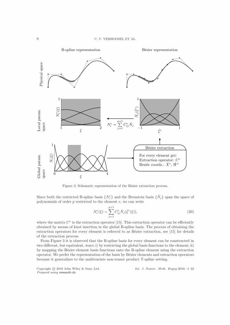
Figure 3. Schematic representation of the Bezier extraction process.

Since both the restricted B-spline basis Nei and the Bernstein basis Nj span the space of

polynomials of order p restricted to the element e, we can write

Nei (ξ) =

p+1∑

j=1

CeijNj(ξ

e(ξ)), (20)

where the matrix Ce is the extraction operator [15]. This extraction operator can be efficientlyobtained by means of knot insertion in the global B-spline basis. The process of obtaining theextraction operators for every element is referred to as Bezier extraction, see [15] for detailsof the extraction process.

From Figure 3 it is observed that the B-spline basis for every element can be constructed intwo different, but equivalent, ways: i) by restricting the global basis functions to the element; ii)by mapping the Bezier element basis functions onto the B-spline element using the extractionoperator. We prefer the representation of the basis by Bezier elements and extraction operatorsbecause it generalizes to the multivariate non-tensor product T-spline setting.



Bezier extraction allows for the construction of a Bezier mesh, over which a higher-ordercontinuous spline basis can be constructed. An analysis suitable Bezier mesh consists of:

• A collection of Bezier elements, each of which is provided with the same set of basisfunctions Nj and a different extraction operator Ce for each element.

• A global set of control point positions, X ∈ Rn×N , and weights, W ∈ R

n, from which theBezier positions and weights can easily be obtained using Xe

i = CejiXj and W e

i = CejiWj .

Since a multivariate Bezier element can be defined as a tensor product of the univariate element,as illustrated in Figure 4 for the bivariate case, the Bezier mesh provides a uniform treatmentof any global spline basis for which extraction operators can be defined. The extraction processhas been studied in detail for univariate and multivariate NURBS [15]. Extraction operatorscan also be derived for multivariate T-spline meshes. Since Bezier extraction operators can beconstructed for T-splines, higher-order continuous Bezier meshes can be created for a largevariety of geometries of engineering interest.

The Bezier extraction operators Ce map the Bezier element basis functions onto a B-splinebasis. In the case that a global NURBS basis is required, the B-spline basis functions aretransformed into NURBS basis functions by equation (17). Since we consider Bezier meshesfor which the global control point positions and weights are provided, this transformation canbe evaluated.

3.3. Isogeometric finite element discretization

Let Su,hi ⊂ Su

i and S η,h ⊂ S η be the discrete solution spaces for the displacement field, u(x),and nonlocal equivalent strain field, η(x), respectively. These spaces are written in terms of thebasis functions defined over the Bezier mesh, Ri(x). We can approximate the displacementfield and nonlocal equivalent strain field as

uhi (x) =

n∑

k=1

Rk(ξ(x))Uki

ηh(x) =n∑

k=1

Rk(ξ(x))Hk

(21)

where U ∈ Rn×N are the control point displacements, and H ∈ R

n the control point nonlocalequivalent strains. From the displacement field, the strain, ε(x), and local equivalent strain,η(x), can be computed. In combination with the nonlocal equivalent strain field, the damageparameter, ω(x), and Cauchy stress, σ(x), can be obtained at every point using the constitutiverelations provided in section 2.1.

We use the Galerkin method to discretize the weak formulation (11) as

(

σij , vu,h(i,j)

)

Ω=(

ti, vu,hi

)

∂Ω∀v

u,hi ∈ Vu,h

i

(

η − η, vη,h)

Ω+

d/2∑

α=1

(

Hαη,Hαvη,h)

Ω= 0 ∀vη,h ∈ V η,h

(22)

Using the NURBS basis functions, Ri(x), as trial functions results in a system of (N + 1)nequations

fum

int,k = fum

ext,k ∀(k, m) ∈ 1 . . . n ⊗ 1 . . .Nf

ηint,k = 0 ∀k ∈ 1 . . . n (23)



-1 -0.5 0 0.5 1 -1-0.5

00.5

100.20.40.60.8

1

N5

ξη

N5

-1 -0.5 0 0.5 1 -1-0.5

00.5

100.20.40.60.8

1

N11

ξη

N11

-1 -0.5 0 0.5 1 -1-0.5

00.5

100.20.40.60.8

1

N12

ξη

N12

-1 -0.5 0 0.5 1 -1-0.5

00.5

100.20.40.60.8

1

N13

ξη

N13

Figure 4. Some basis functions for the bicubic Bezier element. The bivariate basis functions aredefined as the tensor product of two univariate cubic Bezier elements, Na(ξ, η) = Ni(ξ)Nj(η), with

a = (p + 1)(j − 1) + i.

which can be solved for every load step using Newton-Raphson iteration to determine thecontrol point coefficients Uki and Hk in equation (21). The internal force vectors are assembledby looping over the Bezier elements

fum

int,k =

ne

Ae=1

fe,um

int,k =

ne

Ae=1

(

σij ,1

2

(

∂Rek

∂xjδim +

∂Rek

∂xiδjm

))

Ωe

fηint,k =

ne

Ae=1

fe,ηint,k =

ne

Ae=1

(

η − η, Rek

)

Ωe

+

d/2∑

α=1

(

Hαη,HαRek

)

Ωe

(24)

where the element internal force vectors can be expressed in terms of the Bezier basis functions



by substitution of

Reα(ξ) =

Wα

(p+1)N

∑

j=1

CeαjNj(ξ

e(ξ))

n∑

i=1

Wi

(p+1)N∑

j=1

CeijNj(ξe(ξ))

=

Wα

(p+1)N

∑

j=1

CeαjNj(ξ

e(ξ))

(p+1)N∑

j=1

W ej Nj(ξe(ξ))

. (25)

Hence, the internal force vectors can be assembled using the Bezier mesh. The integrals inequation (24) are evaluated on the Bezier elements. In this contribution, we use Gaussianquadrature of order p + 1 in each direction. Numerical integration of NURBS for analysispurposes was studied in [24] and remains an active topic of research. In order to evaluate theintegrals over the Bezier elements, the Jacobian of the isogeometric map needs to be evaluatedat every integration point. Since rational basis functions are used, this requires application ofthe quotient rule. Since higher-order derivatives with respect to the physical coordinate x areused in this contribution, higher-order derivatives of the parametric map are also required (seeAppendix I).

The consistent tangent matrix, required by the Newton-Raphson procedure, can be obtainedby differentiation of (24) with respect to the control point variables in equation (21) to get

Kumut

ks =

ne

Ae=1

Ke,umut

ks , Kumηks =

ne

Ae=1

Ke,umηks , K

ηut

ks =

ne

Ae=1

Ke,ηut

ks , Kηηks =

ne

Ae=1

Ke,ηηks (26)

with

Ke,umut

ks =

(

1

2

(

∂Res

∂xrδqt +

∂Res

∂xqδrt

)

∂σij

∂εqr,1

2

(

∂Rek

∂xjδim +

∂Rek

∂xiδjm

))

Ωe

Ke,umηks =

(

Res

∂σij

∂η,1

2

(

∂Rek

∂xjδim +

∂Rek

∂xiδjm

))

Ωe

Ke,ηut

ks = −(1

2

(

∂Res

∂xrδqt +

∂Res

∂xqδrt

)

∂η

∂εqr, Re

k

)

Ωe

Ke,ηηks =

(

Res, R

ek

)

Ωe

+

d/2∑

α=1

(

HαRes,HαRe

k

)

Ωe

(27)

Upon substitution of equation (25) these element stiffness matrices can be evaluated for everyBezier element. The derivatives of the stress, σ, with respect to the strain, ε, and nonlocalequivalent strain, η, are provided through the constitutive behavior elaborated in section 2.1.The derivative of the local equivalent strain, η, with respect to the strain tensor follows fromthe equivalent strain law, η = η(ε).

4. NUMERICAL SIMULATIONS

4.1. One-dimensional rod loaded in tension

We consider a one-dimensional rod loaded in tension as shown in Figure 5. The 10mm widecentral section of the rod has a reduced cross-sectional area in order to develop a centralized



x

45 mm 10 mm 45 mm

F, u

Figure 5. Schematic representation of a one-dimensional rod loaded in tension. The cross-sectionalarea of the rod is 10 mm2 except for the central section where it is equal to 9mm2.

damage zone. The modulus of elasticity of the rod is E = 20GPa, and the Cauchy stress iswritten as σ = (1 − ω)Eε. As a damage law we consider [7]

ω(κ) =

0 κ ≤ κ0

κu

κκ−κ0

κu−κ0

κ > κ0

(28)

with κ0 = 1 · 10−4 and κu = 0.0125. We define the local equivalent strain law as η = 〈ε〉 where〈·〉 is the Macauley bracket and take the nonlocal length scale in (5) equal to lc =

√2mm.

Force-displacement curves have been determined for the nonlocal damage formulation, andfor the second-, fourth- and sixth-order implicit gradient models. A dissipation-based path-following constraint [25] is used to trace the equilibrium path beyond the snapback point.Mesh convergence studies have been performed using uniform meshes with 80, 160, 320, 640and 1280 linear and cubic Bezier elements (with all control weights equal to 1). An overviewof the meshes is given in Table I. Note that in contrast to higher-order finite elements, thenumber of degrees of freedom is practically independent of the order of the basis.

In Figure 6 we show the force-displacement curves for all formulations obtained on cubicBezier meshes. For the second-order formulation a minor variation in the force-displacementcurve is observed when increasing the number of elements from 640 to 1280. For the higher-order formulations and the nonlocal formulation, the response obtained on the 1280 elementmesh cannot be visually distinguished from that obtained on the 640 element mesh. Thisimproved convergence behavior is attributed to the fact that the higher-order formulationsand nonlocal formulation generate smoother results than the second-order formulation. Theincreased smoothness of the higher-order formulations and the nonlocal formulation is closelyrelated to the postponed loss of ellipticity for these formulations as demonstrated by thedispersion analysis performed in [9]. For the purpose of comparing the various formulations, theaccuracy of the solutions obtained on the 1280 element meshes suffices. In Figure 7 we show theforce-displacment curves for the second-order gradient formulation and nonlocal formulationobtained using linear basis functions. Meaningful results for the higher-order formulationscannot be obtained on these meshes. Comparison of these results with the results obtainedusing cubic B-splines shows the superior convergence behavior of cubic basis functions. Adetailed study of the convergence rates is a topic of future research.

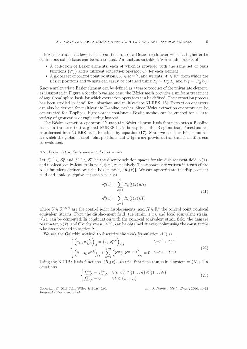
In Figure 8 we show a comparison of the various formulations. All results are obtainedon a cubic Bezier mesh with 1280 elements. The results are in excellent agreement withthose reported in e.g. [7] and [9]. As in [9] it is observed that the incorporation of fourth-order derivatives in the implicit scheme improves the results, in the sense that the obtainedforce-displacement curve is closer to that of the nonlocal formulation. Consistent with thisobservation we find that the sixth-order formulation gives an even better approximation of thenonlocal result. Similar trends are observed from the final damage profiles (see Figure 8). The



Linear Bezier elements (p = 1)Number of elements, ne 80 160 320 640 1280Number of basis functions, n 81 161 321 641 1281

Cubic Bezier elements (p = 3)Number of elements, ne 80 160 320 640 1280Number of basis functions, n 83 163 323 643 1283

Table I. Meshes used for the uniaxial rod simulation.

128064032016080

u [mm]

F[N

]

0.080.060.040.020

20

15

10

5

0

128064032016080

u [mm]

F[N

]

0.080.060.040.020

20

15

10

5

0

(a) (b)

128064032016080

u [mm]

F[N

]

0.080.060.040.020

20

15

10

5

0

128064032016080

u [mm]

F[N

]

0.080.060.040.020

20

15

10

5

0

(c) (d)

Figure 6. Mesh convergence studies for the rod using cubic B-splines for the second-order (a), fourth-order (b) and sixth-order (c) gradient damage formulations, and for the nonlocal formulation (d). The

key labels indicate the number of Bezier elements.



128064032016080

u [mm]

F[N

]

0.080.060.040.020

20

15

10

5

0

128064032016080

u [mm]

F[N

]

0.080.060.040.020

20

15

10

5

0

(a) (b)

Figure 7. Mesh convergence studies for the rod using linear B-splines for the second-order gradient(a) and nonlocal (b) damage formulation. The key labels indicate the number of Bezier elements.

d = 6d = 4d = 2

Nonlocal

u [mm]

F[N

]

0.080.070.060.050.040.030.020.010

20

15

10

5

0

Figure 8. Force-displacement diagrams for the rod loaded in tension using the nonlocal formulationand d-th order gradient formulations. All results are obtained using cubic Bezier meshes with 1280

elements.

sixth-order formulation is found to be very efficient since the results are in good agreementwith the nonlocal formulation, while the involved computational effort is very small comparedto the nonlocal formulation. Based on the resemblance of the sixth-order and nonlocal resultit is concluded that, for the considered simulation, ignoring the nonlocal equivalent strainboundary terms appearing in the gradient formulation has a minor effect on the results.



d = 6d = 4d = 2

Nonlocal

x [mm]

ω[-]

706560555045403530

1

0.8

0.6

0.4

0.2

0

Figure 9. Final damage profile for the rod loaded in tension using the nonlocal formulation and the d-thorder gradient formulations. All results are obtained using cubic Bezier meshes with 1280 elements.

4.2. L-shaped specimen

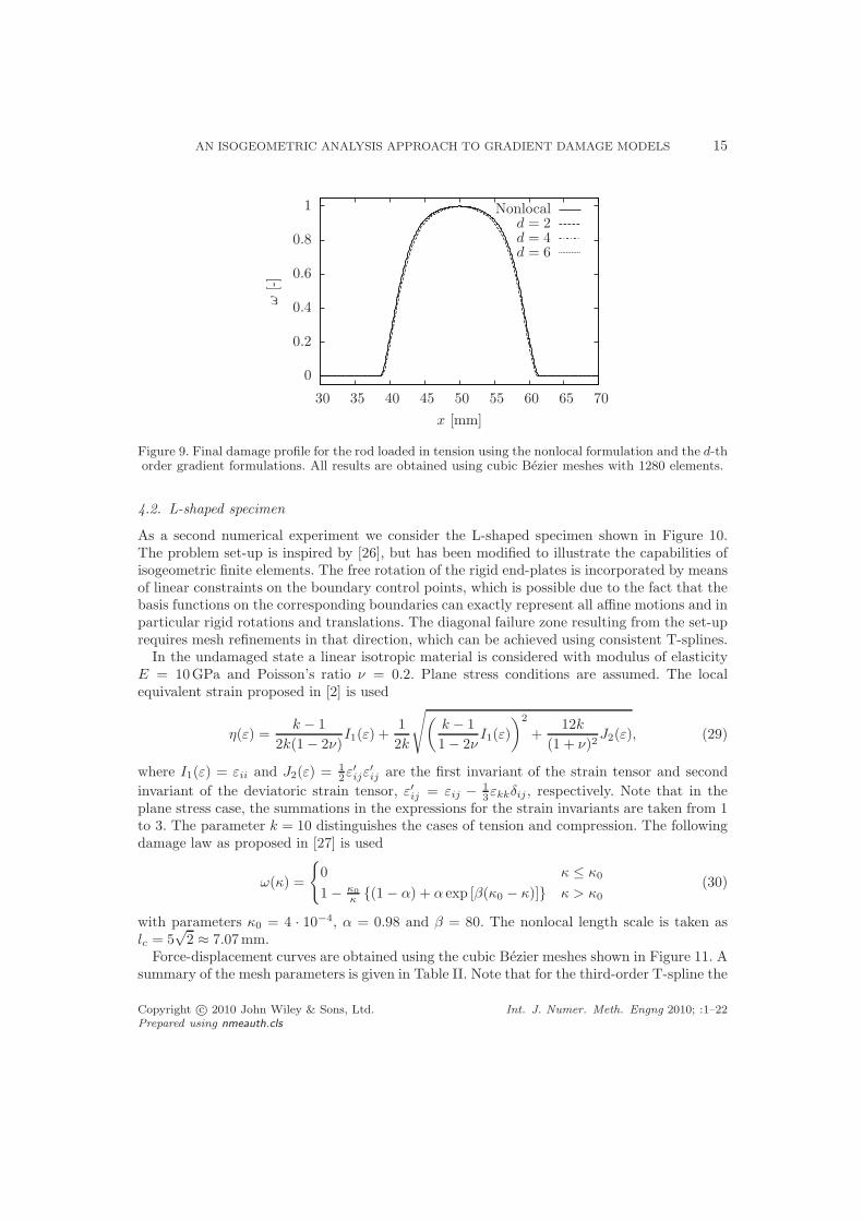
As a second numerical experiment we consider the L-shaped specimen shown in Figure 10.The problem set-up is inspired by [26], but has been modified to illustrate the capabilities ofisogeometric finite elements. The free rotation of the rigid end-plates is incorporated by meansof linear constraints on the boundary control points, which is possible due to the fact that thebasis functions on the corresponding boundaries can exactly represent all affine motions and inparticular rigid rotations and translations. The diagonal failure zone resulting from the set-uprequires mesh refinements in that direction, which can be achieved using consistent T-splines.

In the undamaged state a linear isotropic material is considered with modulus of elasticityE = 10GPa and Poisson’s ratio ν = 0.2. Plane stress conditions are assumed. The localequivalent strain proposed in [2] is used

η(ε) =k − 1

2k(1 − 2ν)I1(ε) +

1

2k

√

(

k − 1

1 − 2νI1(ε)

)2

+12k

(1 + ν)2J2(ε), (29)

where I1(ε) = εii and J2(ε) = 12ε′ijε

′

ij are the first invariant of the strain tensor and second

invariant of the deviatoric strain tensor, ε′ij = εij − 13εkkδij , respectively. Note that in the

plane stress case, the summations in the expressions for the strain invariants are taken from 1to 3. The parameter k = 10 distinguishes the cases of tension and compression. The followingdamage law as proposed in [27] is used

ω(κ) =

0 κ ≤ κ0

1 − κ0

κ (1 − α) + α exp [β(κ0 − κ)] κ > κ0

(30)

with parameters κ0 = 4 · 10−4, α = 0.98 and β = 80. The nonlocal length scale is taken aslc = 5

√2 ≈ 7.07mm.

Force-displacement curves are obtained using the cubic Bezier meshes shown in Figure 11. Asummary of the mesh parameters is given in Table II. Note that for the third-order T-spline the



250

mm

250

mm

250 mm 250 mm

F, u

F, u

Figure 10. L-shaped specimen. The thickness of the specimen is 200 mm.

Mesh 1 Mesh 2 Mesh 3 Mesh 4Spline order, p 3 3 3 3Number of elements, ne 391 816 1686 6032Number of basis functions, n 473 832 1543 5714

Table II. Bezier meshes used for the L-shaped specimen.

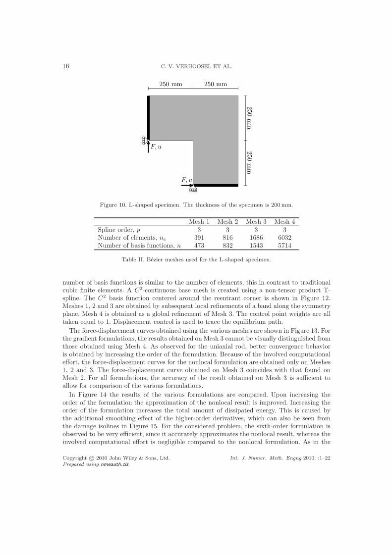
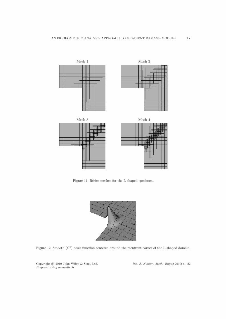
number of basis functions is similar to the number of elements, this in contrast to traditionalcubic finite elements. A C2-continuous base mesh is created using a non-tensor product T-spline. The C2 basis function centered around the reentrant corner is shown in Figure 12.Meshes 1, 2 and 3 are obtained by subsequent local refinements of a band along the symmetryplane. Mesh 4 is obtained as a global refinement of Mesh 3. The control point weights are alltaken equal to 1. Displacement control is used to trace the equilibrium path.

The force-displacement curves obtained using the various meshes are shown in Figure 13. Forthe gradient formulations, the results obtained on Mesh 3 cannot be visually distinguished fromthose obtained using Mesh 4. As observed for the uniaxial rod, better convergence behavioris obtained by increasing the order of the formulation. Because of the involved computationaleffort, the force-displacement curves for the nonlocal formulation are obtained only on Meshes1, 2 and 3. The force-displacement curve obtained on Mesh 3 coincides with that found onMesh 2. For all formulations, the accuracy of the result obtained on Mesh 3 is sufficient toallow for comparison of the various formulations.

In Figure 14 the results of the various formulations are compared. Upon increasing theorder of the formulation the approximation of the nonlocal result is improved. Increasing theorder of the formulation increases the total amount of dissipated energy. This is caused bythe additional smoothing effect of the higher-order derivatives, which can also be seen fromthe damage isolines in Figure 15. For the considered problem, the sixth-order formulation isobserved to be very efficient, since it accurately approximates the nonlocal result, whereas theinvolved computational effort is negligible compared to the nonlocal formulation. As in the



Mesh 1 Mesh 2

Mesh 3 Mesh 4

Figure 11. Bezier meshes for the L-shaped specimen.

Figure 12. Smooth (C2) basis function centered around the reentrant corner of the L-shaped domain.



4321

u [mm]

F[k

N]

2.521.510.50

20

16

12

8

4

0

4321

u [mm]

F[k

N]

2.521.510.50

20

16

12

8

4

0

(a) (b)

4321

u [mm]

F[k

N]

2.521.510.50

20

16

12

8

4

0

321

u [mm]

F[k

N]

2.521.510.50

20

16

12

8

4

0

(c) (d)

Figure 13. Mesh convergence studies using the cubic T-spline meshes in Figure 11 for the second-order(a), fourth-order (b) and sixth-order (c) damage formulations, and for the nonlocal formulation (d).

case of the rod simulation, setting all the Neumann boundary conditions (10) for the equivalentstrain field to zero does not have a significant effect on the results.

5. CONCLUSIONS

Isogeometric analysis allows for the construction of smooth basis functions on complexdomains, providing an appropriate solution space for higher-order differential equations.Dirichlet boundary conditions can be applied by specifying control variables along theboundary, in the same way as nodal variables are specified for traditional finite elements.The higher-order basis functions can be constructed on an element level by means of Bezier



d = 6d = 4d = 2

Nonlocal

u [mm]

F[k

N]

2.521.510.50

20

16

12

8

4

0

Figure 14. Force-displacement results for the L-shaped specimen using the nonlocal formulation andd-th order gradient formulations. All results are obtained using Mesh 3.

Sixth-order

Second-order

Figure 15. Isolines for the damage parameter ω = 0.8 in the L-shaped specimen at u = 2mm ascomputed on Mesh 3 by the second-order formulation and the sixth-order formulation. Displacements

are amplified by a factor of 15.



extraction, which provides compatibility with traditional finite element implementations.

Isogeometric analysis is shown to be a very good candidate for the discretization of higher-order gradient damage formulations. Using cubic basis functions allows for the discretizationof the sixth-order gradient damage formulation. Since, from a practical point of view, thenumber of degrees of freedom is independent of the polynomial order of the basis functions,the fourth- and sixth-order formulation require only slightly more computational effort thanthe second-order formulation. This makes it practical to study the convergence of the implicitgradient damage formulation toward the nonlocal formulation upon increasing its order.

Numerical simulations have been performed for a one-dimensional rod loaded in tension,for which a univariate B-spline basis is constructed. A two-dimensional L-shaped specimenis discretized using Bezier elements, for which the extraction operators have been determinedusing an underlying T-spline. For both simulations it is observed that the result of the nonlocalformulation is approached upon increasing the order of the gradient damage formulation. Sincethe computational effort involved in the nonlocal formulation is much larger than that forthe gradient approximations, increasing the order of the gradient formulation yields efficientapproximations of the nonlocal result. For the two simulations considered, the sixth-orderformulation turned out to give an accurate approximation.

A more detailed study of the mesh convergence behavior of isogeometric finite elements is atopic of further study. In the gradient damage formulations, the approximation behavior, andin particular its dependence on the smoothing length, also needs to be studied in more detail.

ACKNOWLEDGEMENTS

T. J.R. Hughes and M. A. Scott were partially supported by ONR Contract N00014-08-0992, T. J.R.Hughes was also partially supported by NSF Grant 0700204, and M.A. Scott was also partiallysupported by an ICES CAM Graduate Fellowship.

APPENDIX

I. Basis function derivatives

For the assembly of the internal force vector and corresponding tangent, discussed in section 3, thederivatives of the basis function with respect to the physical coordinates are required. In the two-dimensional case, we can compute the first-order derivatives by differentiation of

R(ξ, η) = R(x(ξ, η), y(ξ, η)) (31)

to yield the system„

Rξ

Rη

«

=

»

xξ yξ

xη yη

– „

Rx

Ry

«

(32)

where the subscripts are used to indicate differentiation. Since efficient and robust algorithms existfor the computation of the derivatives with respect to the parametric coordinates, e.g. [21], the basisfunction derivatives with respect to the physical coordinates are obtained by

„

Rx

Ry

«

=1

xξyη − xηyξ

»

yη −yξ

−xη xξ

– „

Rξ

Rη

«

(33)



Using these results, the second-order basis function derivatives with respect to the physical coordinateare obtained by solving the system

2

4

x2

ξ 2xξyξ y2

ξ

xξxη xξyη + xηyξ yξyη

x2

η 2xηyη y2

η

3

5

0

@

Rxx

Rxy

Ryy

1

A =

0

@

Rξξ

Rξη

Rηη

1

A −

2

4

xξξ yξξ

xξη yξη

xηη yηη

3

5

„

Rx

Ry

«

(34)

and subsequently, the third-order derivatives are obtained as

2

6

6

4

x3

ξ 3x2

ξyξ 3xξy2

ξ y3

ξ

x2

ξxη x2

ξyη + 2xξxηyξ xηy2

ξ + 2xξyξyη y2

ξyη

xξx2

η x2

ηyξ + 2xξxηyη xξy2

η + 2xηyξyη yξy2

η

x3

η 3x2

ηyη 3xηy2

η y3

η

3

7

7

5

0

B

B

@

Rxxx

Rxxy

Rxyy

Ryyy

1

C

C

A

=

0

B

@

Rξξξ

Rξξη

Rξηη

Rηηη

1

C

A+

−

2

6

4

3xξxξξ 3xξyξξ + 3xξξyξ 3yξyξξ

2xξxξη + xηxξξ 2xξηyξ + 2xξyξη + xξξyη + xηyξξ 2yξyξη + yηyξξ

2xηxξη + xξxηη 2xξηyη + 2xηyξη + xηηyξ + xξyηη 2yηyξη + yξyηη

3xηxηη 3xηyηη + 3xηηyη 3yηyηη

3

7

5

0

@

Rxx

Rxy

Ryy

1

A +

−

2

6

4

xξξξ yξξξ

xξξη yξξη

xξηη yξηη

xηηη yηηη

3

7

5

„

Rx

Ry

«

(35)

Similar results can be obtained in the three-dimensional case.

REFERENCES

1. Lemaitre J, Chaboche JL. Mechanics of solid materials. Cambridge University Press: Cambridge, 1990.2. de Vree JHP, Brekelmans WAM, van Gils MAJ. Comparison of nonlocal approaches in continuum damage

mechanics. Computers & Structures 1995; 55(4):581–588.3. de Borst R. Encyclopedia of Computational Mechanics, vol. 2: Solids and Structures, chap. 10: Damage,

material instabilities, and failure. Wiley: Chichester, 2004; 335–373.4. Willam KJ, Bicanic N, Stura S. Constitutive and computational aspects of strain-softening and localization

in solids. Constitutive equations: macro and computational aspects, ASME, 1984; 233.5. Brekelmans WAM, de Vree JHP. Reduction of mesh sensitivity in continuum damage mechanics. Acta

Mechanica 1995; 110(1):49–56.6. Pijaudier-Cabot G, Bazant ZP. Nonlocal damage theory. Journal of Engineering Mechanics 1987;

113(10):1512–1533.7. Peerlings RHJ, de Borst R, Brekelmans WAM, de Vree JHP. Gradient enhanced damage for quasi-brittle

materials. International Journal for Numerical Methods in Engineering 1996; 39(19):3391–3403.8. Huerta A, Pijaudier-Cabot G. Discretization influence on regularization by two localization limiters.

Journal of Engineering Mechanics 1994; 120(6):1198–1218.9. Askes H, Pamin J, de Borst R. Dispersion analysis and element-free Galerkin solutions of second-

and fourth-order gradient-enhanced damage models. International Journal for Numerical Methods inEngineering 2000; 49(6):811–832.

10. Sakurai H. Element-free methods vs. mesh-less CAE. International Journal of Computational Methods2006; 3(4):445–464.

11. Hughes TJR, Cottrell JA, Bazilevs Y. Isogeometric analysis: CAD, finite elements, NURBS, exact geometryand mesh refinement. Computer Methods in Applied Mechanics and Engineering 2005; 194(39–41):4135–4195.

12. Cottrell JA, Hughes TJR, Bazilevs Y. Isogeometric Analysis: Toward Integration of CAD and FEA. Wiley:Chichester, 2009.

13. Gomez H, Calo VM, Bazilevs Y, Hughes TJR. Isogeometric analysis of the Cahn-Hilliard phase-field model.Computer Methods in Applied Mechanics and Engineering 2008; 197(49-50):4333–4352.

14. Benson DJ, Bazilevs Y, De Luycker E, Hsu MC, Scott MA, Hughes TJR, Belytschko T. A generalizedfinite element formulation for arbitrary basis functions: from isogeometric analysis to XFEM. InternationalJournal for Numerical Methods in Engineering 2010; DOI: 10.1002/nme.2864.



15. Borden MJ, Scott MA, Evans JA, Hughes TJR. Isogeometric finite element data structures based onBezier extraction. International Journal for Numerical Methods in Engineering 2010; accepted forpublication.

16. Sluys LJ, de Borst R. Dispersive properties of gradient-dependent and rate-dependent media. Mechanicsof Materials 1994; 18(2):131–149.

17. Rogers DF. An Introduction to NURBS. Academic Press: San Diego, 2001.18. Sederberg TW, Zheng J, Bakenov A, Nasri A. T-splines and T-NURCCs. ACM Transactions on Graphics

2003; 22(3):477–484.19. Cox MG. The numerical evaluation of B-splines. IMA Journal of Applied Mathematics 1972; 10(2).20. de Boor C. On calculating with B-splines. Journal of Approximation Theory 1972; 6(1):50–62.21. Piegl L, Tiller W. The NURBS Book. second edn., Springer-Verlag: Berlin, 1997.22. Farin G. Curves and Surfaces for CADG. Academic Press, Inc., 1993.23. Cottrell JA, Hughes TJR, Reali A. Studies of refinement and continuity in isogeometric structural analysis.

Computer Methods in Applied Mechanics and Engineering 2007; 196(41–44):4160–4183.24. Hughes TJR, Reali A, Sangalli G. Efficient quadrature for NURBS-based isogeometric analysis. Computer

Methods in Applied Mechanics and Engineering 2010; 199(5-8):301–313.25. Verhoosel CV, Remmers JJC, Gutierrez MA. A dissipation-based arc-length method for robust simulation

of brittle and ductile failure. International Journal for Numerical Methods in Engineering 2009;77(9):1290–1321.

26. Kuhl E. Numerical models for cohesive frictional materials. PhD Thesis, University of Stuttgart 2000.27. Geers MGD, de Borst R, Brekelmans WAM, Peerlings RHJ. Strain-based transient-gradient damage model

for failure analyses. Computer Methods in Applied Mechanics and Engineering 1998; 160(1-2):133–153.


Documents

ICES REPORT 10-21