IEEE TRANSACTIONS ON GEOSCIENCE AND REMOTE SENSING 1

Deep Feature Extraction and Classification ofHyperspectral Images Based onConvolutional Neural Networks

Yushi Chen, Member, IEEE, Hanlu Jiang, Chunyang Li, Xiuping Jia, Senior Member, IEEE, andPedram Ghamisi, Member, IEEE

Abstract—Due to the advantages of deep learning, in this paper,a regularized deep feature extraction (FE) method is presentedfor hyperspectral image (HSI) classification using a convolutionalneural network (CNN). The proposed approach employs severalconvolutional and pooling layers to extract deep features fromHSIs, which are nonlinear, discriminant, and invariant. Thesefeatures are useful for image classification and target detection.Furthermore, in order to address the common issue of imbalancebetween high dimensionality and limited availability of trainingsamples for the classification of HSI, a few strategies such as L2regularization and dropout are investigated to avoid overfittingin class data modeling. More importantly, we propose a 3-DCNN-based FE model with combined regularization to extracteffective spectral–spatial features of hyperspectral imagery. Fi-nally, in order to further improve the performance, a virtualsample enhanced method is proposed. The proposed approachesare carried out on three widely used hyperspectral data sets:Indian Pines, University of Pavia, and Kennedy Space Center.The obtained results reveal that the proposed models with sparseconstraints provide competitive results to state-of-the-art methods.In addition, the proposed deep FE opens a new window for furtherresearch.

Index Terms—Convolutional neural network (CNN), deeplearning, feature extraction (FE), hyperspectral image (HSI)classification.

I. INTRODUCTION

HYPERSPECTRAL images (HSIs) are usually composedof several hundreds of spectral data channels of the

same scene. The detailed spectral information provided byhyperspectral sensors increases the power of accurately

Y. Chen, H. Jiang, and C. Li are with the Department of Information En-gineering, School of Electronics and Information Engineering, Harbin Instituteof Technology, Harbin 150001, China (e-mail: chenyushi@hit.edu.cn; halo91@163.com; lcy_buzz@mail.dlut.edu.cn).

X. Jia is with the School of Engineering and Information Technology,The University of New South Wales, Canberra, A.C.T. 2600, Australia (e-mail:x.jia@adfa.edu.au).

P. Ghamisi is with Signal Processing in Earth Observation, TechnischeUniversität München, 80333 Munich, Germany, and also with the RemoteSensing Technology Institute (IMF), German Aerospace Center (DLR), 82234Weßling, Germany (e-mail: p.ghamisi@gmail.com).

differentiating materials of interest with increased classificationaccuracy. Moreover, with respect to advances in hyperspectraltechnology, the fine spatial resolution of recently operatedsensors makes the analysis of small spatial structures in imagespossible [1]. The aforementioned advances make the hyper-spectral data a useful tool for a wide variety of applications.By increasing the dimensionality of the images in the spec-tral domain, theoretical and practical problems may arise. Inthis manner, conventional techniques which are developed formultispectral data are no longer efficient for the processingof high-dimensional data mostly due to the so-called curse ofdimensionality [2]. In order to address the curse of dimension-ality, feature extraction (FE) is considered as a crucial step inHSI processing [3]. However, due to the spatial variability ofspectral signatures, HSI FE is still a challenging task [4].

In the early stage of the study on HSI FE, the focus was onspectral-based methods, including principal component analy-sis (PCA) [5], independent component analysis (ICA) [6], lineardiscriminant analysis [7], etc. [8], [9]. These methods applylinear transformations to extract potentially better features ofthe input data in the new domain. With respect to the complexlight-scattering mechanisms of nature objects (e.g., vegetation),hyperspectral data are inherently nonlinear [10], [11], whichmake linear transformation-based methods not that suitable forthe analysis of such data.

Since 2000, when two papers on manifold learning werepublished in Science [12], [13], manifold learning has becomea hot topic in many research areas, including hyperspectralremote sensing. Manifold learning attempts finding the intrinsicstructure of nonlinearly distributed data, which is expected to behighly useful for hyperspectral FE [14].

Alternatively, the nonlinear problem can be addressed bykernel-based algorithms for data representation [15]. Kernelmethods map the original data into a higher dimensional Hilbertspace and offer a possibility of converting a nonlinear problemto a linear one [16].

Recent studies have suggested incorporating spatial informa-tion into a spectral-based FE system [17]. With the developmentof imaging technology, hyperspectral sensors can provide goodspatial resolution. As a result, detailed spatial information hasbecome available [18]. It has been found that spectral–spatialFE methods provide good improvement in terms of classifi-cation performance [19]. In [20], a method was introducedbased on the fusion of morphological operators and supportvector machine (SVM), which leads to high classification

2

accuracy. In [21], the proposed framework extracted the spatialand spectral information using loopy belief propagation andactive learning. The sparse representation [22] of extendedmorphological attribute profile was investigated to incorporatespatial information in remote sensing image classification in[23], which further improves classification accuracy. In thehyperspectral remote sensing community, most of the currentFE methods consider only one-layer processing, which down-grades the capacity of feature learning.

Most of FE and classification methods are not based on a“deep” manner. The widely used PCA and ICA are single-layer learning methods [24]. Classifiers such as linear SVMsand logistic regression (LR) can be attributed as single-layerclassifiers, whereas decision tree or kernel SVMs are believedto have two layers [24].

On the other hand, it is found in neuroscience that the visualsystem of primate human is characterized by a sequence ofdifferent levels of processing (on the order of 10), and this kindof learning system performs very well in the tasks of objectrecognition [25]. Deep learning-based methods, which includetwo or more layers to extract new features, are designed tosimulate the process from the retina to the cortex, and thesedeep architectures have a potential to yield high performancesin image classification and target detection [26], [27].

Undesired scattering from other objects may deform thespectral characteristics of the object of interest. Furthermore,other factors such as different atmospheric scattering conditionsand intraclass variability make it extremely difficult to extractthe features of hyperspectral data effectively. To address suchissues, deep architecture is known as a promising option sinceit can potentially lead to more abstract features at high levels,which are generally robust and invariant [28].

Very recently, some deep models have been proposed forhyperspectral remote sensing image processing [49]. To thebest of our knowledge, a deep learning method, i.e., stackedautoencoder (SAE), was proposed for HSI classification in 2014[29]. Later, an improved autoencoder was proposed based onsparse constraint [50]. In 2015, another deep model, entitleddeep belief network (DBN), was proposed [30]. The deepmodels could extract the robust features and outperform othermethods in terms of classification accuracy. However, due tothe full connection of different layers in the aforementionedapproaches, they demand to train a lot of parameters, whichis an undesirable factor due to the lack of available trainingsamples. Furthermore, SAE and DBN cannot extract the spa-tial information efficiently because they need to represent thespatial information into a vector before the training stage.

Convolutional neural network (CNN) uses local connectionsto effectively extract the spatial information and shared weightsto significantly reduce the number of parameters. Very recently,an unsupervised convolutional network has been proposedfor remote sensing image analysis. This method uses greedylayerwise unsupervised pretraining to formulate a deep CNNmodel [31].

Compared with the unsupervised method, supervised CNNmay extract more effective features with the help of class-specific information, which can be provided by trainingsamples. To extract the spectral and spatial information of

hyperspectral data simultaneously, it is reasonable to formulatea 3-D CNN. Furthermore, to address the problem of over-fitting caused by limited training samples of hyperspectraldata, we design a combined regularization strategy, includingrectified linear unit (ReLU) and dropout to achieve better modelgeneralization.

In this paper, we investigate the application of supervisedCNN, which is one of the deep models, in HSI FE and developa 3-D CNN model for effective spectral-and-spatial-based HSIclassification. It is challenging to apply deep learning to HSIsince its data structure is complex and the number of trainingsamples is limited. In computer vision, the number of trainingsamples varies from tens of thousands to tens of millions [32],[33], whereas having such a large number of training samples isnot common in hyperspectral remote sensing classification. Ingeneral, a neural network has a powerful representation capa-bility with abundant training samples. Without enough trainingsamples, a neural network faces a problem of “overfitting,”which means that the classification performance of test data willbe downgraded. This problem is expected when deep learningis applied to remote sensing data while this paper presents asolution to make such approaches feasible for situations whenonly a limited number of training samples is available. Weuse several regularization methods, including L2 regularization,and dropout strategies to handle the overfitting issue.

The main goal of this paper is to propose a deep FE methodfor HSI classification. With the help of training samples, theproposed CNN models extract the abstract and robust featuresof HSI, which are important for classification. In more detail,the main contributions are listed as follows.

1) Three deep FE architectures based on a CNN are pro-posed to extract the spectral, spatial, and spectral–spatialfeatures of HSI. The designed 3-D CNN can extract thespectral–spatial features effectively, which leads to betterclassification performance.

2) To address the problem of overfitting caused by thelimited number of training samples, some regularizationstrategies, including L2 regularization and dropout, areused in the training process.

3) In order to further improve the performance, a virtualsample enhanced method is proposed to create trainingsamples from the imaging procedure perspective.

4) The hierarchical features of different depth extractedfrom HSI are visualized and analyzed for the first time.

5) The proposed methods are applied on three well-knownhyperspectral data sets. In this context, we compared theproposed methods with some traditional methods froma different perspective such as classification accuracy,analysis of complexities, and processing time.

The remainder of this paper is organized as follows:Section II presents the description of CNN and 1-D CNN-basedHSI spectral FE frameworks. Sections III and IV present thespatial and spectral–spatial FE frameworks for HSI classifica-tion, respectively. The virtual sample enhanced CNN is intro-duced in Section V. The experiments conducted are reported inSection VI. We conclude this paper in Section VII with somediscussions.

3

II. ONE-DIMENSIONAL CNN-BASED

HSI FE AND CLASSIFICATION

A. Neural Network and Deep Learning

How to find effective features is the core issue in imageclassification and pattern recognition. Humans have an amazingskill in extracting meaningful features, and a lot of researchprojects have been undertaken to build an FE system as smartas human in the last several decades. Deep learning is a newlydeveloped approach aiming for artificial intelligence.

Deep learning-based methods build a network with severallayers, typically deeper than three layers. Deep neural network(DNN) can represent complicated data. However, it is verydifficult to train the network. Due to the lack of a proper trainingalgorithm, it was difficult to harness this powerful model untilHinton and Salakhutdinov proposed a deep learning idea [27].

Deep learning involves a class of models that try to learnmultiple levels of data representation, which helps to takeadvantage of input data such as image, speech, and text. Deeplearning model is usually initialized via unsupervised learningand followed by fine-tuning in a supervised manner. The high-level features can be learnt from the low-level features. Thiskind of learning leads to the extraction of abstract and invariantfeatures, which is beneficial for a wide variety of tasks such asclassification and target detection.

There are a few deep learning models in the literature,including DBN [34], [35], SAE [36], and CNN [28]. Recently,CNNs have been found to be a good alternative to other deeplearning models in classification [38], [39] and detection [40].In this paper, we investigate the application of deep CNN forHSI FE.

B. CNN (1-D CNN)

The human visual system can tackle classification, detection,and recognition issues very effectively. Therefore, machinelearning researchers have developed advanced data processingmethods in recent years based on the inspirations from biologi-cal visual systems [25].

CNN is a special type of DNN that is inspired by neuro-science. From Hubel’s earlier work, we know that the cells inthe cortex of the human vision system are sensitive to smallregions. The responses of cells within receptive fields havea strong capability to exploit the local spatial correlation inimages.

Additionally, there are two types of cells within the visualcortex, i.e., simple cells and complex cells. While simple cellsdetect local features, complex cells “pool” the outputs of simplecells within a neighborhood. In other words, simple cells aresensitive to specific edge-like patterns within their receptivefield, whereas complex cells have large receptive fields and theyare locally invariant.

The architecture of CNN is different from other deep learningmodels. There are two special aspects in the architecture ofCNN, i.e., local connections and shared weights. CNN ex-ploits the local correlation using local connectivity betweenthe neurons of near layers. We illustrate this in Fig. 1, wherethe neurons in the mth layer are connected to three adjacent

Fig. 1. Local connections in the architecture of the CNN.

Fig. 2. Shared weights in the architecture of the CNN.

neurons in the (m− 1)th layer, as an example. In CNN, someconnections between neurons are replicated across the entirelayer, which share the same weights and biases. In Fig. 2,the same color indicates the same weight. Using a specificarchitecture like local connections and shared weights, CNNtends to provide better generalization when facing computervision problems.

A complete CNN stage contains a convolution layer and apooling layer. Deep CNN is constructed by stacking severalconvolution layers and pooling layers to form deep architecture.

The convolutional layer is introduced first. The value of aneuron vxij at position x of the jth feature map in the ith layeris denoted as follows:

vxij = g

(bij +

∑m

Pi−1∑p=0

wpijmvx+p

(i−1)m

)(1)

g(x) = tanh(x) =ex − e−x

ex + e−x(2)

where m indexes the feature map in the previous layer ((i−1)th layer) connected to the current feature map, wp

ijm is theweight of position p connected to the mth feature map, Pi isthe width of the kernel toward the spectral dimension, and bijis the bias of jth feature map in the ith layer.

Pooling can offer invariance by reducing the resolution ofthe feature maps [37]. Each pooling layer corresponds to theprevious convolutional layer. The neuron in the pooling layercombines a small N × 1 patch of the convolution layer. Themost common pooling operation is max pooling, which is usedthroughout this paper. The max pooling is as follows:

aj = maxN×1

(an×1i u(n, 1)

)(3)

where u(n, 1) is a window function to the patch of the convo-lution layer, and aj is the maximum in the neighborhood.

All layers, including the convolutional layers and poolinglayers of the deep CNN model, are trained using a back-propagation algorithm.

C. Spectral FE Framework for HSI Classification

In this section, we present a 1-D FE method consideringonly spectral information. This method stacks several CNNs todevelop a deep CNN model with L2 regularization. Generally,the classification of HSI includes two procedures, including FE

4

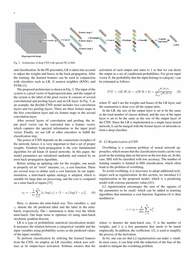
Fig. 3. Architecture of deep CNN with spectral FE of HSI.

and classification. In the FE procedure, LR is taken into accountto adjust the weights and biases in the back-propagation. Afterthe training, the learned features can be used in conjunctionwith classifiers such as LR, K-nearest neighbor (KNN), andSVMs [1].

The proposed architecture is shown in Fig. 3. The input of thesystem is a pixel vector of hyperspectral data, and the output ofthe system is the label of the pixel vector. It consists of severalconvolutional and pooling layers and an LR layer. In Fig. 3, asan example, the flexible CNN model includes two convolutionlayers and two pooling layers. There are three feature maps inthe first convolution layer and six feature maps in the secondconvolution layer.

After several layers of convolution and pooling, the in-put pixel vector can be converted into a feature vector,which captures the spectral information in the input pixelvector. Finally, we use LR or other classifiers to fulfill theclassification step.

The power of CNN depends on the connections (weights) ofthe network; hence, it is very important to find a set of properweights. Gradient back-propagation is the core fundamentalalgorithm for all kinds of neural networks. In this paper, themodel parameters are initialized randomly and trained by anerror back-propagation algorithm.

Before setting an updating rule for the weights, one needsto properly set an “error” measure, i.e., a cost function. Thereare several ways to define such a cost function. In our imple-mentation, a mini-batch update strategy is adopted, which issuitable for large data set processing, and the cost is computedon a mini-batch of inputs [37]

c0 = − 1

m

m∑i=1

[xi log(zi) + (1− xi) log(1− zi)] . (4)

Here, m denotes the mini-batch size. Two variables xi andzi denote the ith predicted label and the label in the mini-batch, respectively. The i summation is done over the wholemini-batch. Our hope turns to optimize (4) using mini-batchstochastic gradient descent.

LR is a type of probabilistic statistical classification model.It measures the relation between a categorical variable and theinput variables using probability scores as the predicted valuesof the input variables.

To perform classification by utilizing the learned featuresfrom the CNN, we employ an LR classifier, which uses soft-max as its output-layer activation. Softmax ensures that the

activation of each output unit sums to 1 so that we can deemthe output as a set of conditional probabilities. For given inputvectorR, the probability that the input belongs to category i canbe estimated as follows:

P (Y = i|R,W, b) = s(WR+ b) =eWiR+bi∑j e

WjR+bj(5)

where W and b are the weights and biases of the LR layer, andthe summation is done over all the output units.

In the LR, the size of the output layer is set to be the sameas the total number of classes defined, and the size of the inputlayer is set to be the same as the size of the output layer ofthe CNN. Since the LR is implemented as a single-layer neuralnetwork, it can be merged with the former layers of networks toform a deep classifier.

D. L2 Regularization of CNN

Overfitting is a common problem of neural network ap-proaches, which means that the classification results can be verygood on the training data set but poor on the test data set. In thiscase, HSI will be classified with low accuracy. The number oftraining samples is limited in HSI classification, which oftenleads to the problem of overfitting.

To avoid overfitting, it is necessary to adopt additional tech-niques such as regularization. In this section, we introduce L2regularization in the proposed model, which is a penalizingmodel with extreme parameter values [41].

L2 regularization encourages the sum of the squares ofthe parameters to be small, which can be added to learningalgorithms that minimize a cost function. Equation (4) is thenmodified to

c = c0 +λ

2m

N∑j=1

w2j (6)

where m denotes the mini-batch size, N is the number ofweights, and λ is a free parameter that needs to be tunedempirically. In addition, the coefficient, 1/2, is used to simplifythe process of the derivation.

In (6), one can see that L2 regularization can make w small.In most cases, it can help with the reduction of the bias of themodel to mitigate the overfitting problem.

5

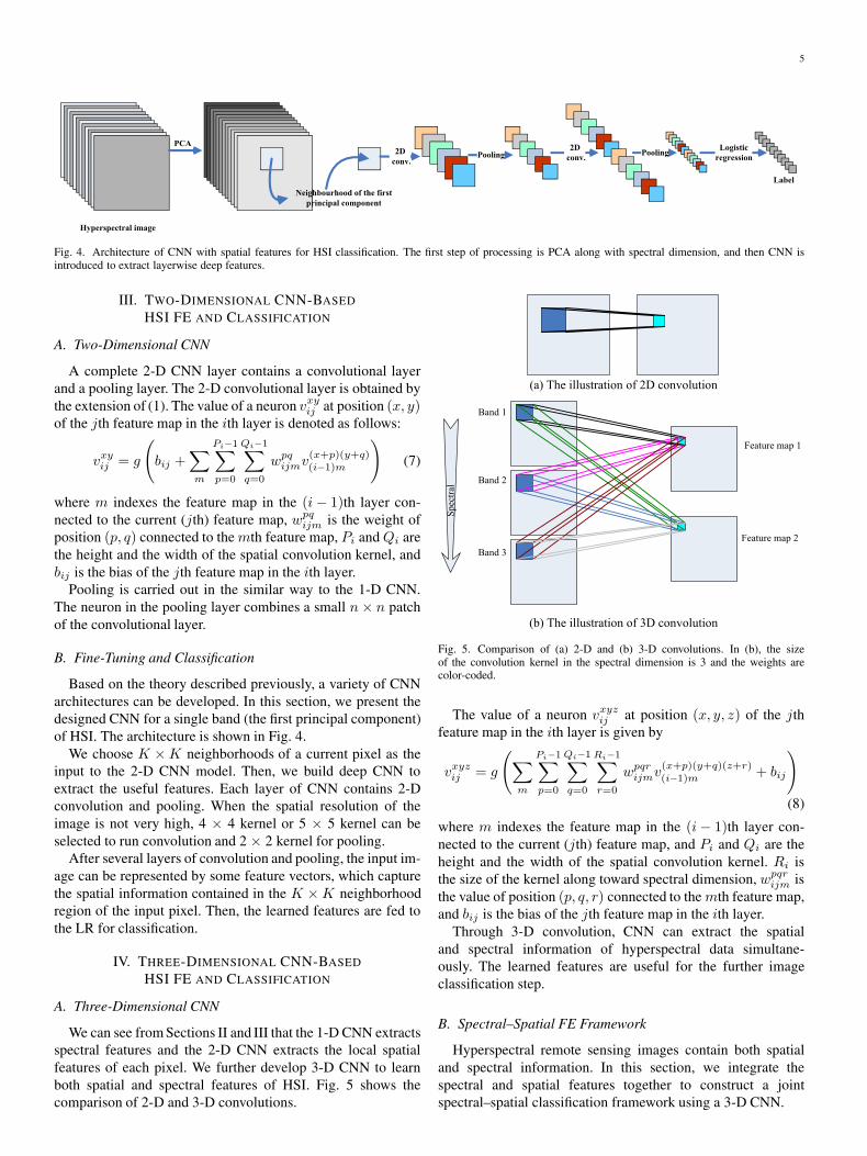
Fig. 4. Architecture of CNN with spatial features for HSI classification. The first step of processing is PCA along with spectral dimension, and then CNN isintroduced to extract layerwise deep features.

III. TWO-DIMENSIONAL CNN-BASED

HSI FE AND CLASSIFICATION

A. Two-Dimensional CNN

A complete 2-D CNN layer contains a convolutional layerand a pooling layer. The 2-D convolutional layer is obtained bythe extension of (1). The value of a neuron vxyij at position (x, y)of the jth feature map in the ith layer is denoted as follows:

vxyij = g

(bij +

∑m

Pi−1∑p=0

Qi−1∑q=0

wpqijmv

(x+p)(y+q)(i−1)m

)(7)

where m indexes the feature map in the (i− 1)th layer con-nected to the current (jth) feature map, wpq

ijm is the weight ofposition (p, q) connected to the mth feature map, Pi and Qi arethe height and the width of the spatial convolution kernel, andbij is the bias of the jth feature map in the ith layer.

Pooling is carried out in the similar way to the 1-D CNN.The neuron in the pooling layer combines a small n× n patchof the convolutional layer.

B. Fine-Tuning and Classification

Based on the theory described previously, a variety of CNNarchitectures can be developed. In this section, we present thedesigned CNN for a single band (the first principal component)of HSI. The architecture is shown in Fig. 4.

We choose K ×K neighborhoods of a current pixel as theinput to the 2-D CNN model. Then, we build deep CNN toextract the useful features. Each layer of CNN contains 2-Dconvolution and pooling. When the spatial resolution of theimage is not very high, 4 × 4 kernel or 5 × 5 kernel can beselected to run convolution and 2 × 2 kernel for pooling.

After several layers of convolution and pooling, the input im-age can be represented by some feature vectors, which capturethe spatial information contained in the K ×K neighborhoodregion of the input pixel. Then, the learned features are fed tothe LR for classification.

IV. THREE-DIMENSIONAL CNN-BASED

HSI FE AND CLASSIFICATION

A. Three-Dimensional CNN

We can see from Sections II and III that the 1-D CNN extractsspectral features and the 2-D CNN extracts the local spatialfeatures of each pixel. We further develop 3-D CNN to learnboth spatial and spectral features of HSI. Fig. 5 shows thecomparison of 2-D and 3-D convolutions.

Fig. 5. Comparison of (a) 2-D and (b) 3-D convolutions. In (b), the sizeof the convolution kernel in the spectral dimension is 3 and the weights arecolor-coded.

The value of a neuron vxyzij at position (x, y, z) of the jthfeature map in the ith layer is given by

vxyzij = g

(∑m

Pi−1∑p=0

Qi−1∑q=0

Ri−1∑r=0

wpqrijmv

(x+p)(y+q)(z+r)(i−1)m + bij

)

(8)

where m indexes the feature map in the (i− 1)th layer con-nected to the current (jth) feature map, and Pi and Qi are theheight and the width of the spatial convolution kernel. Ri isthe size of the kernel along toward spectral dimension, wpqr

ijm isthe value of position (p, q, r) connected to the mth feature map,and bij is the bias of the jth feature map in the ith layer.

Through 3-D convolution, CNN can extract the spatialand spectral information of hyperspectral data simultane-ously. The learned features are useful for the further imageclassification step.

B. Spectral–Spatial FE Framework

Hyperspectral remote sensing images contain both spatialand spectral information. In this section, we integrate thespectral and spatial features together to construct a jointspectral–spatial classification framework using a 3-D CNN.

6

Fig. 6. Architecture of 3-D CNN with spectral–spatial features for HSI classification.

Fig. 6 shows the architecture of 3-D CNN for HSI classi-fication. We choose K ×K ×B neighborhoods of a pixel asan input to the 3-D CNN model, in which B is the numberof bands. Each layer of CNN contains 3-D convolution andpooling. As an example, a 4× 4× 32 kernel or a 5× 5×32 kernel can be applied to 3-D convolution, and a 2 × 2 kernelcan be applied for subsampling. After performing a deep 3-DCNN, the LR approach is conducted for the classification step.

C. Regularizations Based on Sparse Constraints

The issue of high dimensionality and limited number oftraining samples makes the overfitting a serious problem, par-ticularly when the input is a 3-D cube. The dimensionality ofthe spectral-based CNN, which is presented in Section II-C,is around a couple of hundreds (the number of bands); thedimensionality of the spatial-based CNN, which is presented inSection III-B, is around several hundreds (K×K , e.g.,K=27);the dimensionality of the spectral-and-spatial-based CNN,which is presented in Section IV-B, is around several thousands(K ×K ×B). It is easy to obtain that the high dimensionalityof the input data may lead to an overfitting situation. In order tohandle the issue of 3-D CNN, a combined regularization strategybased on sparse constraint is developed, which includes ReLUand dropout, and applies dropout in the fully connected layer.

There are different kinds of ReLUs available to apply. In thispaper, the adopted ReLU is a simple nonlinear operation thataccepts the input of a neuron if it is positive, whereas it returnsto 0 if the input is negative. In many applications, ReLUs inCNNs can improve the performances [42].

Dropout is a recently introduced method to handle overfit-ting. It sets the output of some hidden neurons to zero, whichmeans that the dropped neurons do not contribute in the forwardpass and they are not used in the back-propagation procedure. Indifferent training epochs, the deep CNN forms a different neuralnetwork by dropping neurons randomly. The dropout methodprevents complex co-adaptations [43].

By using ReLU and dropout, the outputs of many neuronsare 0. We use several ReLUs and dropouts at several layers toachieve powerful sparse-based regularization for the deep net-work and address the overfitting problem in HSI classification.

V. VIRTUAL SAMPLE ENHANCED CNN

As a matter of fact, CNN has a lot of weights needed tobe trained. Inappropriate weights may cause getting trapped

in a local minimal of the loss function, which results in poorperformance. To obtain proper weights, a lot of samples arerequired in the training procedure. However, these samplesare usually obtained by manual labeling of a small numberof pixels in an image or based on some field measurements.Therefore, the collection of these samples is both expensiveand time demanding. Consequently, the number of availabletraining samples is usually limited, which is a challenging issuein supervised classification. To solve the dilemma, we utilizevirtual sample as a promising tool from a different perspective.

The virtual sample method tries to create new training sam-ples from given training samples. The critical issue is how togenerate proper samples while we figure out a solution fromthe imaging procedure perspective. Because of the complexsituation of lighting in the large scene, objects of the same classshow different characteristics in different locations. Therefore,we can simulate a virtual sample by multiplying a random fac-tor to a training sample and adding random noise. Furthermore,we can generate a virtual sample from two given samples of thesame class with proper ratios. The virtual sample idea is helpfulin the training of a CNN.

To tackle the problem of having limited training samples,instead of regularization such as L2 regularization and dropout,virtual samples have been generated and added to the trainingsamples.

A. Changing Radiation-Based Virtual Samples

Remote sensing, including hyperspectral imaging, usuallycontains a large scene, whereas the objects of the same classin different locations are affected by different radiation. Virtualsamples can be created by simulating the imaging procedure.New virtual sample yn is obtained by multiplying a randomfactor and adding random noise to a training sample xm

yn = αmxm + βn. (9)

The training sample xm is a cube extracted from the hyper-spectral cube, which contains the spectral and spatial informa-tion of pixel to be classified.

In (9), αm indicates the disturbance of light intensity,which can vary under many situations such as seasons andatmospheric conditions, whereas β controls the weight of therandom Gaussian noise n, which may result from the interac-tion of adjacent pixels and instrumental error.

7

Fig. 7. Indian Pines data set. (Left) False color composite image (bands 28, 19,and 10) and (right) ground truth.

B. Mixture-Based Virtual Samples

Because of the long distance between the object and thesensor, mixture is very common in remote sensing. Inspired bythe phenomenon, it is possible to generate a virtual sample yk

from two given samples of the same class with proper ratios

yk =αixi + αjxj

αi + αj+ βn. (10)

In (10), xi and xj are two training samples from the sameclass, and yk is the virtual sample generated by the two trainingsamples, whereas β controls the weight of the random Gaussiannoise n. Based on the fact that the hyperspectral characteristicsof one class vary within a certain range, it is reasonable toassume that results of mixture within this range still belong tothe same class. Therefore, here, we assign the same label oftraining samples to the virtual sample yk.

Then, the real training samples and virtual samples are usedtogether as training samples to get the proper weights in thenetwork.

Although there are many other methods that can generatethe virtual samples, the changing radiation and mixture-basedmethods are simple yet effective ways.

VI. EXPERIMENTAL RESULTS

A. Data Description and Experiment Design

In our study, three widely used hyperspectral data sets withdifferent environmental settings were adopted to validate theproposed methods. They are a mixed vegetation site over theIndian Pines test area in Northwestern Indiana (Indian Pines),an urban site over the city of Pavia, Italy (University of Pavia),and a site over Kennedy Space Center (KSC), Florida.

The first data set was acquired by the Airborne Visible/Infrared Imaging Spectrometer (AVIRIS). The data set wasobtained from an aircraft flown, with a size of 145 pixels ×145 pixels and 220 spectral bands in the wavelength range of0.4–2.5 μm. The false color image is shown in Fig. 7(a). Thenumber of bands is reduced to 200 by removing water absorp-tion bands. Sixteen different land-cover classes are provided inthe ground truth, as shown in Fig. 7. The number of samples ofeach class is listed in Table I.

The second data set was gathered by a sensor known asthe Reflective Optics System Imaging Spectrometer (ROSIS-3)over the city of Pavia, Italy, with 610 pixels × 340 pixels and115 bands in the range of 0.43–0.86 μm. The high spatial reso-lution of 1.3 m/pixel aims to avoid a high percentage of mixed

TABLE ILAND-COVER CLASSES AND NUMBERS OF PIXELS

ON THE INDIAN PINES DATA SET

Fig. 8. University of Pavia data set. (Left) False color composite (bands 10, 27,and 46) and (right) representing nine land-cover classes.

pixels. In the experiment, noisy bands have been removed andthe remaining 103 channels were used for classification. Nineland-cover classes were selected, which are shown in Fig. 8,and the numbers of samples for each class are given in Table II.

The third data set was acquired by the AVIRIS instrumentover KSC, Florida, on March 23, 1996. The KSC data set hasan altitude of approximately 20 km, with a spatial resolutionof 18 m. The data set includes 176 bands used for the analysisafter removing water absorption and low-signal-to-noise-ratiobands. For classification purposes, 13 classes were defined forthe site. The samples are listed in Table III and shown in Fig. 9.

For all three data sets, we split the labeled samples into twosubsets, i.e., training and test samples, and the details are listedin Tables I–III. During the training procedure of CNN, we used90% of the training samples to learn weights and biases ofeach neuron and the remaining 10% of the training samples toguide the design of proper architectures. In other words, we use

8

TABLE IILAND-COVER CLASSES AND NUMBERS OF PIXELS

ON THE UNIVERSITY OF PAVIA DATA SET

TABLE IIILAND-COVER CLASSES AND NUMBERS

OF PIXELS IN THE KSC DATA SET

Fig. 9. KSC data set. (Left) False color composite (bands 28, 19, and 10) and(right) ground truth.

the classification results of the remaining 10% of the trainingsamples to identify if the network is overfitted. This is importantfor designing the network. The test set is used to assess finalclassification performance.

The experiments were conducted in four scenarios. The firstscenario aims at extracting the deep spectral features of HSI.The second scenario tests the usefulness of deep spatial FE.After this, the effectiveness of deep spectral–spatial FE isinvestigated. In the last scenario, the results of virtual samplemethods are presented.

In order to quantitatively compare the capabilities of the pro-posed models, overall accuracy (OA), average accuracy (AA),

TABLE IVARCHITECTURES OF THE 1-D CNN ON THREE DATA SETS

and Kappa coefficient K are used as performance measures.We run the experiments 20 times with different initial randomtraining samples, and then confidence intervals of OA, AA, andK are reported.

B. Design CNN With Spectral Features

Spectral feature-based HSI classification is a traditional andwidely used method, in which the pixel vector of HSI is theinput. The primary objective of this section is to design a CNNmodel to evaluate the effectiveness of deep FE in the spectraldomain. The experiments include the design and visualizationof spectral information-based CNN and the comparisons withother FE methods and typical classifiers.

1) Architecture Design of the 1-D CNN: Optimization ofCNN was performed using the trial-and-error approach againto determine the parameters of model on the number of nodesin hidden layers, learning rate, kernel size, and the number ofconvolution layers.

Table IV shows the architectures of deep CNNs for three datasets. As an example, for the Indian Pines data set, there are 13layers, denoted as I1, C2, S3, C4, S5, C6, S7, C8, S9, C10,S11, F12, and O13 in sequence. I1 is the input layer. C refersto the convolution layers, and S refers to the pooling layers.F12 is a fully connected layer, and O13 is the output layer ofthe whole neural network.

The input data are normalized into [−1 1]. For the LR, thelearning rate is set to 0.005, and the training epoch is 700 for theIndian Pines data set. For the University of Pavia data set, we setthe learning rate to 0.01 and the number of epochs to 300. Forthe KSC data set, the learning rate is 0.001 with 600 epochs. Ageneralized cross-validation method is applied to estimate thenormalization parameter of L2 regularization [44].

Fig. 10 shows the classification results of the Indian Pines,University of Pavia and KSC data sets. In Fig. 10, we cansee that the depth does help improve classification accuracy.However, too much layers may downgrade classification re-sults. The numbers of proper convolution layers are 5, 3, and 4for the Indian Pines, University of Pavia, and KSC data sets,respectively. This is affected by the dimensionalities of inputs,which are 200, 103, and 176, respectively.

2) Visualization and Analysis of the 1-D CNN: In order to gaindetailed understanding of the 1-D CNN, visualization of CNNforHSI is provided in this section. In the visualization and analysispart, the University of Pavia data set is used as an example.

Weights play a key role in a neural network; hence, they aredisplayed in grayscale images for visualization. Every row inthe figures represents a convolutional kernel, and the intensities

9

Fig. 10. Spectral information-based classification results of different depthsusing CNN.

Fig. 11. Weights of the first convolutional layer on the University of Pavia dataset. Each tiny image (1 × 8) stands for the weights of a convolutional kernel.There are six convolutional kernels in the first convolutional layer. The intensityof each pixel stands for the value of corresponding weight. (a) Randomlyinitialized weights of first convolution layer. (b) Learned weights of firstconvolution layer.

in a row represent the connection intensity of the network. Eachconvolutional kernel can extract the unique feature of the input.Fig. 11 shows the weights of the first convolutional layer on theUniversity of Pavia data set. The weights are randomly ini-tialized and trained using back-propagation methods. FromFig. 11(b), the learned weights show some structures. Forexample, the intensities of the first row are high on the leftside and low on the right side. Fig. 14 shows the weights ofthe 2-D CNN, and it is helpful for the understanding. Differentconvolutional kernels can extract the features from differentperspectives, and the abundant features are helpful for furtherprocessing.

Fig. 12 shows the weights learned at the second and thirdconvolutional layers in an image form where the brightnessis proportional to the value of the weights. There are 12 and24 convolutional kernels at layers 2 and 3, respectively. Thenumbers of weights, i.e., 42 at layer 2 and 96 at layer 3, arearranged in an image form artificially. Different convolutionalkernels can extract the features from different perspectives. Theabundant features are helpful for further processing.

The learned features, which are obtained by the convolutionof inputs and kernels, on the University of Pavia data setare illustrated as curves in Fig. 13. The class of Meadows isselected for visualization, and the extracted features after eachconvolutional layer are shown with a different color. It is shownthat these different features are extracted by different convolu-tion kernels. The extracted features become more abstract afterthe third convolutional and pooling layers.

Fig. 12. Weights of the second and third convolutional layers on the Universityof Pavia data set. In the first column of the image, there are 12 filters, and eachtiny image contains 42(6 × 7) weights of a convolutional kernel. The secondone shows 24 filters and 96(12 × 8) weights in a tiny image. (a) Learnedweights of the second convolutional layer. (b) Learned weights of the thirdconvolutional layer.

In order to evaluate the effectiveness of the extracted fea-tures, the similarity in the same class and the divisibilitybetween different classes are shown in Table V in a quantitativeway. We selected three classes for calculation and calculatedthe divisibility of different classes with J −M distance. TheJ −M distance is defined as [45]

Jij =√2(1− e−Bij ) (11)

Bij =1

8(mi −mj)

T

(ci + cj

2

)−1

(mi −mj)

+1

2log

⎛⎝

∣∣∣ (ci+cj)2

∣∣∣√|ci||cj |

⎞⎠ (12)

wheremi and ci are sample’s average vector and covariance ma-trix. Bij is the Bhattacharyya distance between the two classes.

The similarity in the same class is evaluated with the correla-tion coefficient on a scale of −1 to 1. The correlation coefficientcalculation formula is defined as follows:

ρx,y =C(x, y)√

D(x)√D(y)

(13)

where x and y are two feature vectors, whereas C(x, y) is acovariance matrix. D(x) and D(y) are the variances of twovectors. We use the mean of all correlation coefficients toevaluate the similarity in the same class.

The higher similarity within class and the higher divisibilitybetween classes make the classification step smoother. FromTable V, by comparing the calculated results in different layers,one can see that features have a high similarity in the sameclass and large divisibility in different classes as the number of

10

Fig. 13. Extracted features after convolution and pooling layers on the University of Pavia data set. (a) Original spectral information. (b) and (c) Features afterthe first convolutional layer. (d)–(f) Features after the second convolutional layer. (g)–(i) Features after the third convolutional layer.

TABLE VSIMILARITY AND DIVISIBILITY OF SPECTRAL FEATURES ON THE UNIVERSITY OF PAVIA DATA SET

convolutional layers increases. Therefore, the results infer thatthe extracted features are valid and efficient.

3) Comparisons With Different FE Methods and Classifiers:In this set of experiments, CNN was compared with the PCA, fac-tor analysis (FA), and locally linear embedding (LLE) in order toinvestigate the potential of CNN for hyperspectral spectral FE.PCA is a widely used FE method. FA is a linear statistical methoddesigned for potential factors from observed variables to replaceoriginal data [46]. LLE is a popular nonlinear dimension reduc-tion method, which is considered as a kind of manifold learningalgorithm [47]. In this paper, the effectiveness of different FEmethods is evaluated mainly through classification results. Wealso classify the features using several classifiers such as KNNclassifier and a nonlinear SVM based on radial basis function(RBF-SVM). Using the same features with different classifiers,we can evaluate the effectiveness of the extracted features.

Tables VI–VIII show that the CNN-based FE methods al-ways provide the best performances of OA, AA, and Kappa forall three data sets. The classification accuracy values are givenin the form of mean ± standard deviation from the perspectiveof statistics, which is used as a measurement of volatility.

In order to have a fair comparison, we used 10% of the trainingsamples to find the best parameters of FE methods using gridsearch. The result reported in Tables VI–VIII are the best classifi-cation results when the number of features was properly selectedfor each FE method. On the selection of parameters, the numberof features was chosen in the range of 10 to N (i.e., the numberof hyperspectral bands) with an interval of 10. The number ofneighbors in LLE has been changed in a range from 1 to 10. Thefinal classification results such as OA, AA, and Kappa were cal-culated on the test data set. In this set of experiments, CNN wascompared with the PCA, FA, and LLE in order to investigate thepotential of CNN for hyperspectral spectral FE. PCA is a widelyused FE method. FA is a linear statistical method designed forpotential factors from observed variables to replace original data[46]. LLE is a popular nonlinear dimension reduction method,which is considered as a kind of manifold learning algorithm[47]. In this paper, the effectiveness of different FE methods isevaluated mainly through classification results. We also classifythe features using several classifiers such as KNN classifier andan RBF-SVM. Using the same features with different classi-fiers, we can evaluate the effectiveness of the extracted features.

11

TABLE VICLASSIFICATION RESULTS OBTAINED BY DIFFERENT FE APPROACHES ON THE INDIAN PINES DATA SET

TABLE VIICLASSIFICATION RESULTS OBTAINED BY DIFFERENT FE APPROACHES ON THE UNIVERSITY OF PAVIA DATA SET

12

TABLE VIIICLASSIFICATION RESULTS OBTAINED BY DIFFERENT FE APPROACHES ON THE KSC DATA SET

Tables VI–VIII show that the CNN-based FE methods al-ways provide the best performances of OA, AA, and Kappa forall three data sets. The classification accuracy values are givenin the form of mean ± standard deviation from the perspectiveof statistics, which is used as a measurement of volatility.

In order to have a fair comparison, we used 10% of the train-ing samples to find the best parameters of FE methods usinggrid search. The result reported in Tables VI–VIII are the bestclassification results when the number of features was properlyselected for each FE method. On the selection of parameters,the number of features was chosen in the range of 10 to N (i.e.,the number of hyperspectral bands) with an interval of 10. Thenumber of neighbors in LLE has been changed in a range from1 to 10. For KNN, the range of the nearest neighbors has beenchanged from 1 to 30 with the interval of two. In RBF-SVM,there are two parameters, i.e., C and γ [48]; thus, we applied2-D grid search from a wide range (i.e., C=2−5, 2−4, . . . , 219;γ = 2−15, 2−14, . . . 24) to get the best parameters. The learningrate and the number of epochs for LR were selected empirically.

Table VI also shows the results obtained in a situation whenthe models were trained using the original complete set ofspectral bands (200 bands) of the Indian Pines data set. Dueto the imbalance between the numbers of training samples andthe numbers of bands used, the accuracy and its correspondingvariance have a wide range from one class to another one.Compared with PCA, FA, and LLE, CNN-based FE leads tobetter performance, particularly when it combines with LR.The CNN-LR exhibits the highest OA, AA, and K , the highestpercentage of correctly classified pixels among all the test

TABLE IXARCHITECTURE OF THE 2-D CONVOLUTION NEURAL NETWORK

pixels considered, with an improvement of 3.92%, 3.88%, and0.046 over the RBF-SVM, respectively.

Table VII shows the experimental results for the Universityof Pavia data set. It is shown that the CNN-LR provides betterresults again and outperforms RBF-SVM by 2.26%, 2.39%, and0.0237 on average in terms of OA, AA, andK , respectively. It isworth noting that the obtained variance is very small. In terms ofclass accuracy values, the class “Bricks” was the most difficultone to be classified. The CNN-LR still exhibits the best accuracy(89.09 ± 1.18) for this class. Concerning computational cost,CNN has the longest processing time (given by the sum of thetraining and test times) compared with the other methods.

C. CNN With Spatial Features

In this section, we investigate the effectiveness of the 2-DCNN for hyperspectral data FE and classification. There aretwo reasons. On one hand, the original CNN is designed for 2-Dimage classification. The usefulness of 2-D CNN for HSI classi-fication should be tested. In this paper, 1-D CNN and 3-D CNNare designed for spectral classification and spectral–spatialclassification, respectively. On the other hand, to maintain theintegrity, 2-D CNN should be investigated. There are several

13

Fig. 14. Weights of the first convolutional layer. Each tiny image (4 × 4) stands for a convolutional kernel. There are 32 kernels in the first convolutional layer.The intensity of each pixel stands for the value of corresponding weight. (a) Randomly initialized weights of the first convolution layer of the University of Paviadata set. (b) Learned weights of the first convolution layer of the University of Pavia data set.

Fig. 15. Extracted features of the University of Pavia data set. There are six rows, and each row of images represents one class. There are four columns in thefigure. The first column is allocated to the input images. The second column is allocated to the four feature maps after the first convolution. The third column isallocated to the four feature maps after the first ReLU operation. The last column is composed of the four features of the first pooling operation.

approaches to create 2-D input such as choose one band of HSIrandomly. The first principal component is used to create the2-D input because the first principal component contains themost energy of the whole HSI. The learned spatial features areused for further classification.

1) Architecture Design, Visualization, and Analysis: Thereare several factors that need to be selected in the experiments.The input images were normalized into [−0.5 0.5]. We useda large neighborhood window (27 × 27) for the first principalcomponent as the input 2-D image for the three data sets.

The details of the architecture of the CNN are listed inTable IX. Because of the small size of the input image, weused three convolution layers and three pooling layers. Afterthe CNN, the input image was converted into a vector with128 dimensions.

In the training procedure, we used a mini-batch-based back-propagation method, whereas the size of mini-batch is 100.The learning rate of all CNNs is set to be 0.01. In this partof the experiment, the number of training epochs of the CNNis 200.

Fig. 16. Extracted features after three convolutional layers on two asphaltsamples. The number of feature maps after the first convolution layer is 32,and the size of each feature map is 24 × 24; the number of feature maps afterthe second convolution layer is 64, and the size of each feature map is 8 × 8;and the number of feature maps after the second convolution layer is 128, andthe size of each feature map is 1 × 1.

14

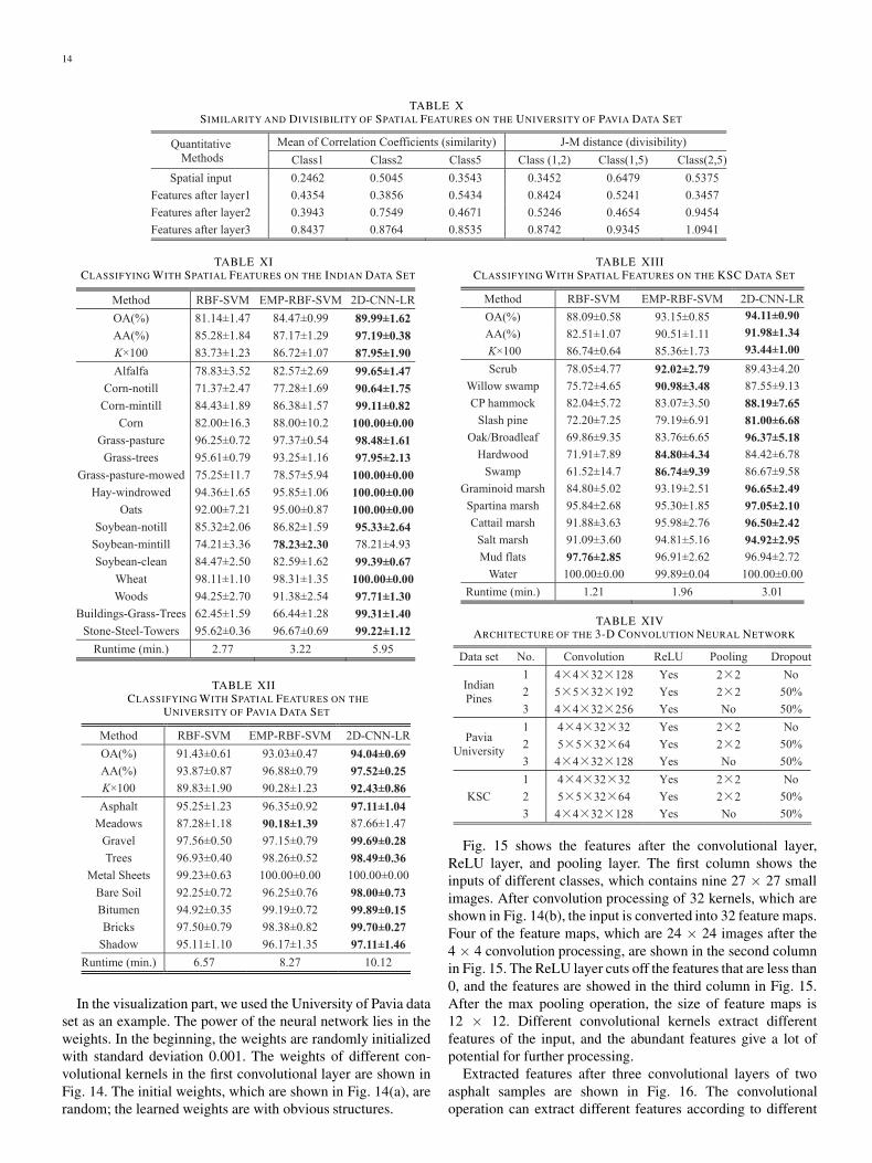
TABLE XSIMILARITY AND DIVISIBILITY OF SPATIAL FEATURES ON THE UNIVERSITY OF PAVIA DATA SET

TABLE XICLASSIFYING WITH SPATIAL FEATURES ON THE INDIAN DATA SET

TABLE XIICLASSIFYING WITH SPATIAL FEATURES ON THE

UNIVERSITY OF PAVIA DATA SET

In the visualization part, we used the University of Pavia dataset as an example. The power of the neural network lies in theweights. In the beginning, the weights are randomly initializedwith standard deviation 0.001. The weights of different con-volutional kernels in the first convolutional layer are shown inFig. 14. The initial weights, which are shown in Fig. 14(a), arerandom; the learned weights are with obvious structures.

TABLE XIIICLASSIFYING WITH SPATIAL FEATURES ON THE KSC DATA SET

TABLE XIVARCHITECTURE OF THE 3-D CONVOLUTION NEURAL NETWORK

Fig. 15 shows the features after the convolutional layer,ReLU layer, and pooling layer. The first column shows theinputs of different classes, which contains nine 27 × 27 smallimages. After convolution processing of 32 kernels, which areshown in Fig. 14(b), the input is converted into 32 feature maps.Four of the feature maps, which are 24 × 24 images after the4 × 4 convolution processing, are shown in the second columnin Fig. 15. The ReLU layer cuts off the features that are less than0, and the features are showed in the third column in Fig. 15.After the max pooling operation, the size of feature maps is12 × 12. Different convolutional kernels extract differentfeatures of the input, and the abundant features give a lot ofpotential for further processing.

Extracted features after three convolutional layers of twoasphalt samples are shown in Fig. 16. The convolutionaloperation can extract different features according to different

15

Fig. 17. Classification results with and without dropout on the (left) Indian Pines, (middle) University of Pavia, and (right) KSC data sets.

Fig. 18. Training error with and without ReLU on the (left) Indian Pines, (middle) University of Pavia, and (right) KSC data sets.

convolutional kernels. The correlation coefficient of the two in-put images is 0.2975, which means that they are quite different.After three convolutions, the correlation coefficient of the twoinputs is 0.8324, which means they are quite similar. This kindof processing is very useful for further classification.

In order to evaluate the effectiveness of the extracted fea-tures, the similarity in the same class and the divisibilitybetween the different classes are shown in Table X in a quan-titative way. From Table X, after convolution operations, thesimilarity in the same class and the divisibility in differentclasses are increased. While some features in the middle layershave relatively low similarity in the same class and relativelylow divisibility in the different classes, the features in themiddle layers are not suitable for classification.

In Tables XI–XIII, we can see that the deep CNN methodoutperforms RBF-SVMs in terms of the OA, AA, and Kappa.In this case, the CNN significantly improves RBF-SVM for allthree data sets.

D. CNN With Spatial–Spectral Features

In this part of the experiments, we investigate the advantageof 3-D CNN for HSI FE and classification. With the help ofproper CNN architecture, we used the neighbors of the pixel inall bands. The CNN learns the spectral and spatial features byitself, and learned features were used in classification.

Fig. 19. Influence of spatial size on the (left) Indian Pines, (middle) Universityof Pavia, and (right) KSC data sets. Best view in color.

1) Architecture Design and Parameter Analysis: For theIndian Pines, University of Pavia, and KSC data sets, we use27× 27× 200, 27× 27× 103, and 27× 27× 176 neighborsof each pixel as the input 3-D images, respectively. The inputimages are normalized into [−0.5 0.5]. The structures’ detailsare given in Table XIV. After the 3-D CNN, the input imagewas converted into a vector. The size of mini-batch was 100,

16

TABLE XVSIMILARITY AND DIVISIBILITY OF SPECTRAL–SPATIAL FEATURES ON THE UNIVERSITY OF PAVIA DATA SET

and the learning rate was 0.003. In this set of experiments, thenumber of training epochs CNNs is 400.

There are three factors (dropout, ReLU, and the size of thespatial window) that influence the final classification accuracysignificantly, and they are analyzed in the following.

In the proposed architecture, dropout plays an importantrole to address overfitting. In this experiment, the results(classification error) with and without dropout on the three datasets are presented in Fig. 17. In the figure, the training errorswithout dropout regularization are very low after dozens ofepochs, whereas the test errors without dropout are very high.This is the problem of overfitting. For the training and test errorswith dropout, the training errors are relatively high, whereas thetest errors are relatively low. This means that the model withdropout has a good capability of generalization.

The effectiveness of the dropout can be explained in twoways. The first one is to prevent co-adaptations of the unitson the training samples, and the second one is to average thepredictions of many different networks [43]. If a hidden unitknows its collaborative units, it leads to good performance onthe training data. However, these units might not perform wellon the test data set. However, if a hidden unit adapts well onmany different collaborative units, it will be more dependenton itself rather than depending on some certain combinationsof hidden units. Dropout strategy makes it possible to traindifferent networks, and each network gets a classification result.As the training procedure continues, most of the networks givethe correct results to eliminate incorrect results on the finalclassification results.

ReLU is another important factor that is influential to finalperformance. Krizhevsky et al. claimed that the nonsaturatingnonlinear function as ReLU can gain better performances thanthese saturating nonlinearities such as sigmoid function [26].The classification errors with and without ReLU on the threedata sets are demonstrated in Fig. 18. From Fig. 18, conver-gence of the models with sigmoid function are slower thanconvergence of the models with ReLU. In particular, on theIndian Pines data set, a CNN with ReLU (red solid lines)reaches a 50% error rate six times faster than the same networkwith sigmoid (blue dashed lines). On the other hand, the modelswith ReLU can lead to lower training error (close to 0) at theend of training. In summary, CNN with ReLU can accelerateconvergence and improve the training accuracy.

The size of 3-D input is an important parameter too. Thedimensionality toward spectral dimension is fixed, whereas thedimensionalities toward spatial dimension are changeable. Aset of experiments is organized to get a proper size of 3-D inputs.Fig. 19 shows the results using different sizes of spatial window.The half widths of spatial size are set to W =[11, 12, 13, 14, 15],

TABLE XVICLASSIFICATION WITH SPECTRAL–SPATIAL FEATURES

ON THE INDIAN PINES DATA SET

and the full width is 2W + 1. To have a fair comparison, weresize other spatial sizes to 27 × 27 and get classificationaccuracy values using the models aforementioned. For theIndian Pines data set, the OA can reach the highest and the valueis nearly 98% when the half width is 14. For the University ofPavia and KSC data sets, the results show that the best accuracyvalues are obtained when the half width is 13.

In order to evaluate the effectiveness of the extractedspectral–spatial features, Table XV presents the similarity inthe same class and the divisibility between the different classes.Compared with Tables V and X, after convolution operations,the spectral–spatial features get the highest similarity in thesame class and the highest divisibility between the differentclasses, which shows that the spectral–spatial features have thepotential for accurate classification.

2) Comparative Experiments With Other Spectral–SpatialMethods: We also conducted RBF-SVM with the original datasets and extended morphological profile (EMP) for compari-son. EMP followed by SVM is an advanced spatial–spectralclassification method for hyperspectral data. We used openingand closing operations on the first five, seven, and three prin-cipal components of the Indian Pines, University of Pavia, andKSC data sets to extract structural information, respectively. Inthe experiments, the structuring element used was a disk and

17

TABLE XVIICLASSIFICATION WITH SPECTRAL–SPATIAL FEATURES

ON THE UNIVERSITY OF PAVIA DATA SET

TABLE XVIIICLASSIFICATION WITH SPECTRAL–SPATIAL

FEATURES ON THE KSC DATA SET

the structure sizes were progressively increased from 1 to 4.Therefore, 40, 56, and 24 spatial features were generated. Thegenerated spatial features and original spectral features are usedfor classification. Wide ranges of c and g values for the SVMwere searched in the EMP with the RBF-SVM method; for theIndian Pines data set, they were configured as c = 218 and g =21, whereas those in the Pavia data set were c = 219 and g = 21,and in the KSC data set, they were c = 210 and g = 2−1.

Tables XVI–XVIII provide information about the classifica-tion results compared with the typical SVMs. From the results,we can see that the classification accuracy values of CNN in termsof OA, AA, and Kappa coefficient are higher than those of otherFE and classification methods. The results show that the de-signed CNN can help improve the classification accuracy of HSI.

3) Computation Cost of the 3-D CNN: In general, we con-cede that neural networks take longer time to train the networkcompared with other machine learning algorithms such as KNNor SVM, and so does the proposed deep learning methods.

TABLE XIXRUNNING TIME COMPARISON

TABLE XXCLASSIFICATION ACCURACY VALUES ON THE INDIAN PINES DATA SET

TABLE XXICLASSIFICATION ACCURACY VALUES ON THE

UNIVERSITY OF PAVIA DATA SET

TABLE XXIICLASSIFICATION ACCURACY VALUES ON THE KSC DATA SET

On the other hand, the advantage of deep learning algorithmsis that they are superfast on testing.

The training and test times are shown in Table XIX. In the ta-ble, we can see that the test time is only 0.88, 1.02, and 0.30 minfor the Indian Pines, University of Pavia, and KSC data sets,respectively. Fast test time is very important in real applications.

With the quick development of hardware technology, par-ticularly on graphic processing units, the drawback of longtraining time of a deep learning method can be mitigated in thenear future.

E. CNN With Virtual Sample

1) Classification Results: In this part of the experiments, theadvantages of 3-D CNN with virtual samples for HSI FE andclassification are investigated. The two proposed virtual samplemethods (Method A and Method B) in Section V are tested onthe three data sets.

For every virtual sample generated by (9), αm is a uniformlydistributed random number in [0.9, 1.1], and β, which is theweight of noise n, is set to 1/25. Meanwhile, for every virtualsample generated by (10), αi and αj are uniformly distributedrandom numbers on the interval [0, 1], whereas xi and xj arerandomly chosen from the same class.

The CNN architecture and the training procedure in thissection are the same as in the previous section. Classificationaccuracy values obtained by different approaches on the IndianPines, University of Pavia, and KSC data sets are shown inTables XX–XXII.

18

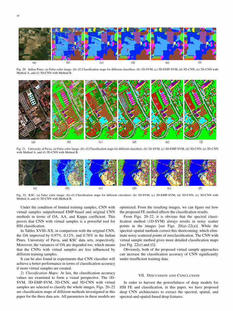
Fig. 20. Indian Pines. (a) False color image. (b)–(f) Classification maps for different classifiers: (b) 1D-SVM, (c) 3D-EMP-SVM, (d) 3D-CNN, (e) 3D-CNN withMethod A, and (f) 3D-CNN with Method B.

Fig. 21. University of Pavia. (a) False color image. (b)–(f) Classification maps for different classifiers: (b) 1D-SVM, (c) 3D-EMP-SVM, (d) 3D-CNN, (e) 3D-CNNwith Method A, and (f) 3D-CNN with Method B.

Fig. 22. KSC. (a) False color image. (b)–(f) Classification maps for different classifiers: (b) 1D-SVM, (c) 3D-EMP-SVM, (d) 3D-CNN, (e) 3D-CNN withMethod A, and (f) 3D-CNN with Method B.

Under the condition of limited training samples, CNN withvirtual samples outperformed EMP-based and original CNNmethods in terms of OA, AA, and Kappa coefficient. Thisproves that CNN with virtual samples is a powerful tool forHSI classification.

In Tables XVIII–XX, in comparison with the original CNN,the OA improved by 0.97%, 0.12%, and 0.76% in the IndianPines, University of Pavia, and KSC data sets, respectively.Moreover, the variances of OA are degraded too, which meansthat the CNNs with virtual samples are less influenced bydifferent training samples.

It can be also found in experiments that CNN classifier willachieve a better performance in terms of classification accuracyif more virtual samples are created.

2) Classification Maps: At last, the classification accuracyvalues are examined to form a visual perspective. The 1D-SVM, 3D-EMP-SVM, 3D-CNN, and 3D-CNN with virtualsamples are selected to classify the whole images. Figs. 20–22are classification maps of different methods investigated in thispaper for the three data sets. All parameters in these models are

optimized. From the resulting images, we can figure out howthe proposed FE method affects the classification results.

From Figs. 20–22, it is obvious that the spectral classi-fication method (1D-SVM) always results in noisy scatterpoints in the images [see Figs. 20(a)–22(a)]. While thespectral–spatial methods correct this shortcoming, which elim-inate noisy scattered points of misclassification. The CNN withvirtual sample method gives more detailed classification maps[see Fig. 22(e) and (f)].

Obviously, both of the proposed virtual sample approachescan increase the classification accuracy of CNN significantlyunder insufficient training data.

VII. DISCUSSION AND CONCLUSION

In order to harvest the powerfulness of deep models forHSI FE and classification, in this paper, we have proposeddeep CNN architectures to extract the spectral, spatial, andspectral-and-spatial-based deep features.

19

The design of proper deep CNN models is the first importantissue we are facing. In the design of the spectral deep model,we use a small local reception field and three to five convolu-tional layers. For the spatial deep model, we use a small localreception field. For the spectral-and-spatial-based deep model,we use a special 3-D CNN model with a large reception fieldin the spectral domain and a small reception field in the spatialdomain to extract the integrated features of HSI. The properdesign will balance the capacity and complexity of the network,which is very important for further FE and classification.

In hyperspectral remote sensing cases, only limited trainingsamples are available. To solve the problem of overfitting, weuse L2 regularization for spectral CNN. When the input is a 3-Dcube, overfitting becomes more serious. We then adopt a regu-larization entitled dropout. The proper regularization strategiesplay an important role for accurate classification of HSI.

Parameters affect the classification accuracy and computa-tional complexity. In the realization of deep CNNs for HSIFE and classification, we gather some useful experience onparameter setting. The experimental results suggest that oneor two layers often provide limited capacity in FE of HSI.Based on our experimental results, we suggest using a three-layer CNN with 4 × 4 or 5 × 5 convolution kernel and 2 × 2pooling kernel in each layer for HSI FE.

By using proper architecture and powerful regularization, theproposed 3-D deep CNN has been demonstrated to provide excel-lent classification performance under the condition of limitedtraining samples. The proposed deep model is promising withhigh potential, which opens a new window for further research.

In order to further improve the performance of CNN-basedmethods, a method entitled virtual sample is proposed. Virtualsamples are generated by changing radiation and different mix-ture. Then, the training samples and the created virtual samplesare used together in order to train a CNN.

In summary, to address the HSI FE and classification prob-lem with limited training samples, we propose an idea of bignetwork with strong constraints. The big feedforward DNNusing deep 3-D CNN with virtual samples achieves by far thebest results in terms of classification accuracy.

CNN is a hot topic in machine learning and computer vi-sion. Various improvements have been made in recent years,and they can be also used in the proposed CNN architecture.The proposed model can be combined with post-classificationprocessing to enhance mapping performance. It deserves to beinvestigated as a possible future work.

REFERENCES

[1] J. A. Benediktsson and P. Ghamisi, Spectral–Spatial Classification of Hy-perspectral Remote Sensing Images. Boston, MA, USA: Artech House,2015.

[2] G. Hughes, “On the mean accuracy of statistical pattern recognizers,”IEEE Trans. Inf. Theory, vol. IT-14, no. 1, pp. 55–63, Jan. 1968.

[3] J. B. Dias et al., “Hyperspectral remote sensing data analysis and futurechallenges,” IEEE Geosci. Remote Sens. Mag., vol. 1, no. 2, pp. 6–36,Feb. 2013.

[4] X. Jia, B. Kuo, and M. M. Crawford, “Feature mining for hyperspectralimage classification,” Proc. IEEE, vol. 101, no. 3, pp. 676–679,Mar. 2013.

[5] G. Licciardi, P. R. Marpu, J. Chanussot, and J. A. Benediktsson, “Linearversus nonlinear PCA for the classification of hyperspectral data based onthe extended morphological profiles,” IEEE Geosci. Remote Sens. Lett.,vol. 9, no. 3, pp. 447–451, May 2011.

[6] A. Villa, J. A. Benediktsson, J. Chanussot, and C. Jutten, “Hyperspectralimage classification with independent component discriminant analysis,”IEEE Trans. Geosci. Remote Sens., vol. 49, no. 12, pp. 4865–4876,Dec. 2011.

[7] T. V. Bandos, L. Bruzzone, and G. Camps-Valls, “Classification of hy-perspectral images with regularized linear discriminant analysis,” IEEETrans. Geosci. Remote Sens., vol. 47, no. 3, pp. 862–873, Mar. 2009.

[8] L. M. Bruce, C. H. Koger, and J. Li, “Dimensionality reduction ofhyperspectral data using discrete wavelet transform feature extraction,”IEEE Trans. Geosci. Remote Sens., vol. 40, no. 10, pp. 2331–2338,Oct. 2002.

[9] L. O. Jimenez and D. A. Landgrebe, “Hyperspectral data analysis andsupervised feature reduction via projection pursuit,” IEEE Trans. Geosci.Remote Sens., vol. 37, no. 6, pp. 2653–2667, Nov. 1999.

[10] D. Lunga, S. Prasad, M. M. Crawford, and O. Ersoy, “Manifold-learning-based feature extraction for classification of hyperspectral data: A reviewof advances in manifold learning,” IEEE Signal Process. Mag., vol. 31,no. 1, pp. 55–66, Jan. 2014.

[11] T. Han, and D. Goodenough, “Investigation of nonlinearity in hyperspec-tral imagery using surrogate data methods,” IEEE Trans. Geosci. RemoteSens., vol. 46, no. 10, pp. 2840–2847, Oct. 2008.

[12] B. Tenenbaum, V. Silva, and C. Langford, “A global geometric frameworkfor nonlinear dimensionality reduction,” Science, vol. 290, no. 5500,pp. 2319–2323, Dec. 2000.

[13] S. Roweis and L. K. Saul, “Nonlinear dimensionality reduction bylocally linear embedding,” Science, vol. 290, no. 5500, pp. 2323–2326,Dec. 2000.

[14] C. M. Bachmann, T. L. Ainsworth, and R. A. Fusina, “Improved man-ifold coordinate representations of large-scale hyperspectral scenes,”IEEE Trans. Geosci. Remote Sens., vol. 44, no. 10, pp. 2786–2803,Oct. 2006.

[15] B. Scholkopf and A. J. Smola, Learning With Kernels. Cambridge, MA,USA: MIT Press, 2002.

[16] B. C. Kuo, C. H. Li, and J. M. Yang, “Kernel nonparametric weightedfeature extraction for hyperspectral image classification,” IEEE Trans.Geosci. Remote Sens., vol. 47, no. 4, pp. 1139–1155, Apr. 2009.

[17] A. Plaza, J. Plaza, and G. Martin, “Incorporation of spatial constraints intospectral mixture analysis of remotely sensed hyperspectral data,” in Proc.IEEE Int. Workshop Mach. Learn. Signal Process., Grenoble, France,2009, pp. 1–6.

[18] M. Fauvel, Y. Tarabalka, J. A. Benediktsson, J. Chanussot, andJ. C. Tilton, “Advances in spectral–spatial classification of hyperspectralimages,” Proc. IEEE, vol. 101, no. 3, pp. 652–675, Mar. 2013.

[19] Y. Tarabalka, M. Fauvel, J. Chanussot, and J. A. Benediktsson, “SVM- andMRF-based method for accurate classification of hyperspectral images,”IEEE Geosci. Remote Sens. Lett., vol. 7, no. 4, pp. 736–740, Oct. 2010.

[20] M. Fauvel, J. A. Benediktsson, J. Chanussot, and J. Sveinsson, “Spectraland spatial classification of hyperspectral data using SVMs and mor-phological profiles,” IEEE Trans. Geosci. Remote Sens., vol. 46, no. 11,pp. 3804–3814, Nov. 2008.

[21] J. Li, J. M. Bioucas-Dias, and A. Plaza, “Spectral–spatial classifica-tion of hyperspectral data using loopy belief propagation and activelearning,” IEEE Trans. Geosci. Remote Sens., vol. 51, no. 2, pp. 844–856,Feb. 2013.

[22] Y. Chen, N. M. Nasrabadi, and T. D. Tran, “Hyperspectral image classifi-cation using dictionary-based sparse representation,” IEEE Trans. Geosci.Remote Sens., vol. 49, no. 10, pp. 3973–3985, Oct. 2011.

[23] B. Song, J. Li, J. M. Bioucas-Dias, and J. A. Benediktsson, “Remotelysensed image classification using sparse representations of morphologicalattribute profiles,” IEEE Trans. Geosci. Remote Sens., vol. 52, no. 8,pp. 5122–5136, Aug. 2013.

[24] Y. Bengio, A. Courville, and P. Vincent, “Representation learning. Areview and new perspectives,” IEEE Trans. Pattern Anal. Mach. Intell.,vol. 35, no. 8, pp. 1798–1828, Aug. 2013.

[25] N. Kruger et al., “Deep hierarchies in primate visual cortex what canwe learn for computer vision?” IEEE Trans. Pattern Anal. Mach. Intell.,vol. 35, no. 8, pp. 1847–1871, Aug. 2013.

[26] A. Krizhevsky, I. Sutskever, and G. Hinton, “ImageNet classification withdeep convolutional neural networks,” in Proc. Neural Inf. Process. Syst.,Lake Tahoe, NV, USA, 2012, pp. 1106–1114.

[27] G. Hinton and R. Salakhutdinov, “Reducing the dimensionality of datawith neural networks,” Science, vol. 313, no. 5786, pp. 504–507, Jul. 2006.

[28] Y. LeCun, L. Bottou, Y. Bengio, and P. Haffner, “Gradient-based learn-ing applied to document recognition,” Proc. IEEE, vol. 86, no. 11,pp. 2278–2324, Nov. 1998.

[29] Y. Chen, Z. Lin, X. Zhao, and G. Wang, “Deep learning-based classifi-cation of hyperspectral data,” IEEE J. Sel. Topics Appl. Earth Observ.Remote Sens., vol. 7, no. 6, pp. 2094–2107, Jun. 2014.

20

[30] Y. Chen, X. Zhao, and X. Jia, “Spectral–spatial classification of hyper-spectral data based on deep belief network,” IEEE J. Sel. Topics Appl.Earth Observ. Remote Sens., vol. 8, no. 6, pp. 1–12, Jun. 2015.

[31] A. Romero, C. Gatta, and G. Camps-Valls, “Unsupervised deep featureextraction for remote sensing image classification,” IEEE Trans. Geosci.Remote Sens., vol. 54, no. 3, pp. 1349–1362, Mar. 2016.

[32] Y. LeCun, C. Cortes, and C. Burges, The MNIST Database of HandwrittenDigits. [Online]. Available: http://yann.lecun.com/exdb/mnist/

[33] J. Deng and F. Li, “ImageNet: A large-scale hierarchical image database,”in Proc. CVPR, Miami, FL, USA, 2009, pp. 248–255.

[34] G. E. Hinton, S. Osindero, and Y. Teh, “A fast learning algorithm for deepbelief nets,” Neural Comput., vol. 18, no. 7, pp. 1527–1554, Jul. 2006.

[35] N. LeRoux and Y. Bengio, “Deep belief networks are compact uni-versal approximators,” Neural Comput., vol. 22, no. 8, pp. 2192–2207,Aug. 2010.

[36] P. Vincent, H. Larochelle, I. Lajoie, Y. Bengio, and P. Manzagol,“Stacked denoising autoencoders,” J. Mach. Learn. Res., vol. 11, no. 12,pp. 3371–3408, Dec. 2010.

[37] Z. Zuo et al., “Learning contextual dependence with convolutional hier-archical recurrent neural networks,” IEEE Trans. Image Process., vol. 25,no. 7, pp. 2983–2996, Jul. 2016.

[38] C. Szegedy et al., “Going deeper with convolutions,” in Proc. IEEECVPR, Boston, MA, USA, 2015, pp. 1–9.

[39] K. Simonyan and A. Zisserman, “Very deep convolutional networks forlarge-scale image recognition,” in Proc. ICLR, 2015, pp. 1–14.

[40] R. Girshick, J. Donahue, T. Darrell, and J. Malik, “Rich feature hierarchiesfor accurate object detection and semantic segmentation,” in Proc. IEEECVPR, Columbus, OH, USA, 2014, pp. 581–587.

[41] A. E. Hoerl and R. W. Kennard, “Ridge regression: Biased estimationfor non-orthogonal problems,” Technimetrics, vol. 12, no. 1, pp. 55–67,Jan. 1970.

[42] V. Nair and G. E. Hinton, “Rectified linear units improve restrictedBoltzmann machines,” in Proc. Int. Conf. Mach. Learn., Haifa, Israel,2010, pp. 807–814.

[43] G. E. Hinton et al., “Improving neural networks by preventing co-adaptation of feature detectors,” Comput. Sci., vol. 3, no. 4, pp. 212–223,2012.

[44] R. E. Edwards, H. Zhang, and L. E. Parker, “Approximate l-fold cross-validation with least squares SVM and kernel ridge regression,” in Proc.12th ICMLA, Miami, FL, USA, Dec. 2013, pp. 58–64.

[45] W. Hofmann, “Remote sensing: The quantitative approach,” IEEE Trans.Pattern Anal. Mach. Intell., vol. 3, no. 6, pp. 713–714, Jun. 1981.

[46] D. J. Bartholomew, F. Steele, J. Galbraith, and I. Moustaki, “Analysis ofmultivariate social science data,” Struct. Equation Model. Multidiscipli-nary J., vol. 18, no. 4, pp. 686–693, Apr. 2011.

[47] H. Yang, F. Qin, and Y. Wang, “LLE-PLS nonlinear modeling method fornear infrared spectroscopy and its application,” Spectrosc. Spectral Anal.,vol. 27, no. 10, pp. 1955–1958, Oct. 2007.

[48] C. Chang and C. Lin, “LIBSVM: A library for support vector machines,”ACM Trans. Intell. Syst. Technol., vol. 2, no. 3, pp. 1–27, Mar. 2011.

[49] L. G. Chova, D. Tuia, G. Moser, and G. C. Valls, “Multimodal classifi-cation of remote sensing images: A review and future directions,” Proc.IEEE, vol. 103, no. 9, pp. 1560–1584, Nov. 2015.

[50] C. Tao, H. Pan, Y. Li, and Z. Zou, “Unsupervised spectral–spatial fea-ture learning with stacked sparse autoencoder for hyperspectral im-agery classification,” IEEE Geosci. Remote Sens. Lett., vol. 12, no. 12,pp. 2438–2442, Dec. 2015.

[51] J. A. Benediktsson, J. A. Palmason, and J. R. Sveinsson, “Classificationof hyperspectral data from urban areas based on extended morphologicalprofiles,” IEEE Trans. Geosci. Remote Sens., vol. 43, no. 3, pp. 480–491,Mar. 2005.

Yushi Chen (M’11) received the Ph.D. degree fromthe Harbin Institute of Technology, Harbin, China,in 2008.

Currently, he is an Associate Professor with theSchool of Electronics and Information Engineering,Harbin Institute of Technology. His research interestsinclude remote sensing data processing and machinelearning.

Hanlu Jiang received the Bachelor’s degree in re-mote sensing science and technology in 2014 fromthe Harbin Institute of Technology, Harbin, China,where she is currently working toward the Master’sdegree in the School of Electronics and InformationEngineering.

Her research area is in remote sensing imageprocessing technologies.

Chunyang Li has been working toward the Master’sdegree in the Department of Information Engineer-ing, School of Electronics and Information Engineer-ing, Harbin Institute of Technology, Harbin, China,since 2015.

Her research concerns remote sensing imageprocessing based on deep learning methods.

Xiuping Jia (SM’03) received the B.Eng. degreefrom the Beijing University of Posts and Telecom-munications, Beijing, China, in 1982 and the Ph.D.degree in electrical engineering from The Universityof New South Wales, Sydney, Australia, in 1996.

Since 1988, she has been with the School ofEngineering and Information Technology, The Uni-versity of New South Wales, Canberra, Australia,where she is currently a Senior Lecturer. She is also aGuest Professor with Harbin Engineering University,Harbin, China, and an Adjunct Researcher with the

National Engineering Research Center for Information Technology in Agricul-ture, Beijing. She is the coauthor of the remote sensing textbook titled RemoteSensing Digital Image Analysis [Springer-Verlag, 3rd ed. (1999) and 4th ed.(2006)]. Her research interests include remote sensing and image data analysis.

Dr. Jia served as the inaugural Chair of the IEEE Australia Capital Territoryand New South Wales Section GRSS Chapter from 2010 to 2013. She isan Associate Editor of the IEEE TRANSACTIONS ON GEOSCIENCE AND

REMOTE SENSING.

Pedram Ghamisi (S’12–M’15) received the B.Sc.degree in civil (survey) engineering from the IslamicAzad University, South Tehran Branch, Tehran, Iran;the M.Sc. degree (with first class honors) in re-mote sensing from Khajeh Nasir Toosi University ofTechnology, Tehran, in 2012; and the Ph.D. degreein electrical and computer engineering from theUniversity of Iceland, Reykjavik, Iceland, in 2015.

He was a Postdoctoral Research Fellow with theUniversity of Iceland. Since October 2015, he hasbeen a Postdoctoral Research Fellow with Signal

Processing in Earth Observation, Technical University of Munich, Munich,Germany, and a Researcher with the Remote Sensing Technology Institute(IMF), German Aerospace Center (DLR), Weßling, Germany. His researchinterests are in remote sensing and image analysis with special focus on spectraland spatial techniques for hyperspectral image classification and the integrationof LiDAR and hyperspectral data for land-cover assessment.

In 2015, Dr. Ghamisi won the prestigious Alexander von HumboldtFellowship.