Embed Size (px)
Citation preview
ORNL/TM-2015/314
Impact of Measurement Error on Synchrophasor Applications
Jiecheng Zhao Jin Tan Ling Wu Lingwei Zhan Yilu Liu Jose R. Gracia Paul D. Ewing
July 2015
Approved for public release: distribution is unlimited.
DOCUMENT AVAILABILITY
Reports produced after January 1, 1996, are generally available free via US Department of Energy (DOE) SciTech Connect. Website http://www.osti.gov/scitech/ Reports produced before January 1, 1996, may be purchased by members of the public from the following source: National Technical Information Service 5285 Port Royal Road Springfield, VA 22161 Telephone 703-605-6000 (1-800-553-6847) TDD 703-487-4639 Fax 703-605-6900 E-mail [email protected] Website http://www.ntis.gov/help/ordermethods.aspx Reports are available to DOE employees, DOE contractors, Energy Technology Data Exchange representatives, and International Nuclear Information System representatives from the following source: Office of Scientific and Technical Information PO Box 62 Oak Ridge, TN 37831 Telephone 865-576-8401 Fax 865-576-5728 E-mail [email protected] Website http://www.osti.gov/contact.html
This report was prepared as an account of work sponsored by an agency of the United States Government. Neither the United States Government nor any agency thereof, nor any of their employees, makes any warranty, express or implied, or assumes any legal liability or responsibility for the accuracy, completeness, or usefulness of any information, apparatus, product, or process disclosed, or represents that its use would not infringe privately owned rights. Reference herein to any specific commercial product, process, or service by trade name, trademark, manufacturer, or otherwise, does not necessarily constitute or imply its endorsement, recommendation, or favoring by the United States Government or any agency thereof. The views and opinions of authors expressed herein do not necessarily state or reflect those of the United States Government or any agency thereof.
ORNL/TM-2015/314
Electrical and Electronics Systems Research Division
IMPACT OF MEASUREMENT ERROR ON SYNCHROPHASOR APPLICATIONS
Jiecheng Zhao*
Jin Tan*
Ling Wu*
Lingwei Zhan*
Yilu Liu†*
Jose R. Gracia†
Paul D. Ewing†
*University of Tennessee, Knoxville †Oak Ridge National Laboratory
Date Published: July 2015
Prepared by
OAK RIDGE NATIONAL LABORATORY
Oak Ridge, TN 37831-6283
managed by
UT-BATTELLE, LLC
for the
US DEPARTMENT OF ENERGY
under contract DE-AC05-00OR22725

iii
CONTENTS
LIST OF FIGURES ...................................................................................................................................... v
LIST OF TABLES ....................................................................................................................................... vi
ACRONYMS .............................................................................................................................................. vii
ACKNOWLEDGMENTS ........................................................................................................................... ix
ABSTRACT .................................................................................................................................................. 1
1. INTRODUCTION ................................................................................................................................ 1
1.1 PHASOR MEASUREMENT UNIT APPLICATIONS .............................................................. 1
1.2 PHASOR MEASUREMENT UNIT ERRORS .......................................................................... 2
1.3 INSTRUMENTATION CHANNEL ERRORS .......................................................................... 2
1.4 ASSUMPTIONS IN THIS REPORT ......................................................................................... 3
2. IMPACT ON EVENT LOCATION ..................................................................................................... 5
2.1 APPROACH ............................................................................................................................... 5
2.2 NORTHEAST POWER COORDINATING COUNCIL MODEL-BASED
SIMULATION ............................................................................................................................ 6
2.3 REAL-EVENT-BASED SIMULATION ................................................................................. 10
2.4 SUMMARY OF EVENT LOCATION IMPACT .................................................................... 16
3. IMPACT ON OSCILLATION DETECTION .................................................................................... 17
3.1 APPROACH ............................................................................................................................. 17
3.2 RESULTS AND ANALYSIS ................................................................................................... 19
3.3 SUMMARY OF OSCILLATION DETECTION IMPACT ..................................................... 21
4. IMPACT ON ISLANDING DETECTION......................................................................................... 23
4.1 APPROACH ............................................................................................................................. 23
4.2 RESULTS AND ANALYSIS ................................................................................................... 24
4.3 SUMMARY OF ISLANDING DETECTION IMPACT .......................................................... 28
5. IMPACT ON DYNAMIC LINE RATING ........................................................................................ 29
5.1 APPROACH ............................................................................................................................. 29
5.2 RESULTS AND ANALYSIS ................................................................................................... 31
5.2.1 Scenario 1..................................................................................................................... 31 5.2.2 Scenario 2..................................................................................................................... 33 5.2.3 Scenario 3..................................................................................................................... 35
5.3 SUMMARY OF DYNAMIC LINE RATING IMPACT .......................................................... 36
6. CONCLUSION ................................................................................................................................... 37
7. REFERENCES ................................................................................................................................... 39
APPENDIX A. APPLICATIONS OF PHASOR MEASUREMENT UNITS .......................................... A-1
APPENDIX B. DYNAMIC LINE RATING MODEL ............................................................................. B-1
APPENDIX C. INPUT DATA FOR DYNAMIC LINE RATING MODEL ........................................... C-1

v
LIST OF FIGURES
1.1. Typical instrumentation channel for a phasor measurement unit ........................................................ 3
2.1. Angle curves with error band .............................................................................................................. 6
2.2. Northeast Power Coordinating Council model ................................................................................... 7
2.3. Angle curves of the first six buses ...................................................................................................... 8
2.4. Angle curves of the first six buses with ±0.15 error .......................................................................... 8
2.5. Angle curves of the first six buses with ±0.6 error ............................................................................ 9
2.6. Triangulation failure caused by 1.2 error .......................................................................................... 9
2.7. The processed phase angle curves measured by frequency difference recorders in a
generation trip event.......................................................................................................................... 10
2.8. Phase angle curves of 2010/01/03 generation trip............................................................................. 11
2.9. Phase angle curves of 2010/03/14 generation trip............................................................................. 11
2.10. Phase angle curves of 2010/07/16 generation trip............................................................................. 12
2.11. Phase angle curves of 2011/05/09 generation trip............................................................................. 12
2.12. Phase angle curves of 2011/06/26 generation trip............................................................................. 13
2.13. Phase angle curves of 2011/10/12 generation trip............................................................................. 13
2.14. Angle curves of 03/12/2010 event .................................................................................................... 14
2.15. Angle curves of 03/12/2010 event with 0.1 error ............................................................................ 14
2.16. Angle curves of 03/12/2010 event with ±0.6 error .......................................................................... 15
2.17. Triangulation failure caused by 1.2 error ........................................................................................ 15
3.1. Angle measurement vs. frequency measurement in oscillation detection ......................................... 18
3.2. Schematic of the angle-based oscillation detection ........................................................................... 19
3.3. Phasor measurement unit error impact on an oscillation signal ........................................................ 19
3.4. Phasor measurement unit error impact on a nonoscillation signal .................................................... 20
3.5. Phasor measurement unit error impact on oscillation signal ............................................................. 21
4.1. Flow chart of the islanding detection method ................................................................................... 24
4.2. Frequency measured by frequency disturbance recorders in the
Hurricane Sandy case ........................................................................................................................ 25
4.3. Frequency with 0.35 Hz error in the Hurricane Sandy case .............................................................. 25
4.4. Frequencies measured by frequency disturbance recorders in the
2010/06/01 Western Electricity Coordinating Council islanding case ............................................. 26
4.5. Frequencies with 0.2 Hz error in the 2010/06/01 Western Electricity
Coordinating Council islanding case ................................................................................................ 26
4.6. Frequencies measured by frequency disturbance recorders in the
2010/07/22 Western Electricity Coordinating Council islanding case ............................................. 27

vi
4.7. Frequencies with 0.2Hz error in the 2010/07/22 Western Electricity
Coordinating Council islanding case ................................................................................................ 27
5.1. Transmission line with phasor measurement units at both ends ....................................................... 29
5.2. Overall framework of phasor measurement unit (PMU)–based
dynamic line rating technology ......................................................................................................... 30
5.3. Dynamic line rating error on 1 day in summer ................................................................................. 34
5.4. Dynamic line rating error on 1 day in winter .................................................................................... 34
5.5. Impact of wind speed, temperature, and solar heat gain on
dynamic line rating error ................................................................................................................... 35
LIST OF TABLES
5.1. Phasor measurement unit error impact on dynamic line rating with
different error directions ................................................................................................................... 31
7.1. Effect of measurement error on applications .................................................................................... 37

vii
ACRONYMS
ACSR aluminum conductor, steel-reinforced
ADC analog-to-digital converter
CT current transformer
CCVT capacitive coupled voltage transformer
DFT discrete Fourier transform
DG distributed generation
DLR dynamic line rating
EI Eastern Interconnection
FD frequency deviation
FDR frequency disturbance recorder
FNET Frequency Monitoring Network
GPS Global Positioning System
IOFD integration of frequency deviation
LSB least significant bit
NPCC Northeast Power Coordinating Council
PSD power spectral density
PMU phasor measurement unit
PPS pulse-per-second
PSS/E Siemens Power System Simulator for Engineering
RMS root mean square
SLR static line rating
SNR signal-to-noise ratio
TDOA time difference of arrival
THD total harmonic distortion
TVE total vector error
UTC Coordinated Universal Time
VT voltage transformer
WECC Western Electricity Coordinating Council


ix
ACKNOWLEDGMENTS
The authors would like to thank Ye Zhang [University of Tennessee–Knoxville (UTK)], Dao Zhou
(UTK), Jiahui Guo (UTK), Gefei, Kou (UTK), Dr. Kai Sun (UTK), Denis Osipov (UTK), David
Bertagnolli (ISO New England) and Kyle Thomas (Dominion Virginia Power) for discussions and
technical assistance in creating this report. The authors would also like to acknowledge the careful and
detailed review on language by Samantha White (UTK) and technical editing by Vj Ewing (Oak Ridge
National Laboratory).

1
ABSTRACT
Phasor measurement units (PMUs), a type of synchrophasor, are powerful diagnostic tools that can help
avert catastrophic failures in the power grid. Because of this, PMU measurement errors are particularly
worrisome. This report examines the internal and external factors contributing to PMU phase angle and
frequency measurement errors and gives a reasonable explanation for them. It also analyzes the impact of
those measurement errors on several synchrophasor applications: event location detection, oscillation
detection, islanding detection, and dynamic line rating. The primary finding is that dynamic line rating is
more likely to be influenced by measurement error. Other findings include the possibility of reporting
nonoscillatory activity as an oscillation as the result of error, failing to detect oscillations submerged by
error, and the unlikely impact of error on event location and islanding detection.
1. INTRODUCTION
First introduced in the 1980s, synchronized phasor measurement units (PMUs) have now become a
mature technology used for many applications essential to power system efficiency and integrity (see
Appendix A). Linked in synchronized networks, PMUs are capable of reflecting the status of the whole
measured power system and are useful for power system stability monitoring, postmortem analysis, and
adaptive protection and control and to improve efficiency and lower costs. The measurement of frequency
and phase angle, which is used by most applications, is subject to measurement errors from both internal
and external factors, which may influence the accuracy of the applications or even cause their failure.
This report analyzes the range of PMU measurement errors and then discusses their influence on several
applications.
Measurement errors typically originate in the PMU and instrumentation channels between the power line
and the PMU. In this section, errors from these two sources are discussed and assumptions for the error
impacts are given.
1.1 PHASOR MEASUREMENT UNIT APPLICATIONS
PMUs, a kind of synchrophasor, were developed to monitor and analyze power system behavior. The
device provides a way to monitor a wide-area power system with very high precision in both distance and
time, through the use of its high resolution and time synchronization. Compared to many traditional
power system devices, PMUs provide precise frequency and phase angle measurement results. This
feature is the basis of many applications for power system monitoring and protection.
Event location estimation is one PMU application. When events such as generation trip or load shedding
occur, a sudden mismatch of active power will happen and cause a significant frequency and phase angle
increase or decrease depending on the event type. Because these perturbations travel through the grid as
electromechanical waves dispersing at finite speeds, PMUs located throughout the grid are able to detect
the variation of frequency and angle with unique time delays proportional to the distance from the PMU
to the disturbance. Applications based on this have been developed to estimate the event location [1].
Oscillation detection is another PMU application. Disturbances ranging from a small amount of load
variation to the loss of a large generator typically evoke voltage, angle, and frequency oscillations in the
power system. A system that lacks sufficient ability to damp oscillations can become unstable and even
experience cascading blackouts. It wasn’t until the advent of PMUs that oscillations could be easily
observed [2]. Similar to generation trip events, frequency oscillations propagate through the system as
electromechanical waves and therefore can be observed by PMUs.
2
As distributed generation (DG) has been more broadly used, it has brought new kinds of problems, one of
the most important of which is islanding. Islanding is the situation where a distributed energy resource
continues to supply loads when the DG system is disconnected from the utility power system. An
islanding occurrence not only poses a threat to power quality and the safety of maintenance crews, but
may also seriously damage the DG network and delay restoration [3–5]. When islanding occurs, the
islanded part cannot synchronize with the bulk power system, and therefore, a frequency difference
between the two parts occurs. By detecting this difference, PMUs can discover the islanding event.
Dynamic line rating (DLR) is used to evaluate the maximum allowable currents of the transmission line in
real time. It is essential to maximizing use of the transmission line while avoiding equipment degradation
or failure [6]. Using PMUs for DLR can save the cost of installing additional devices while providing
real-time, accurate results [7].
1.2 PHASOR MEASUREMENT UNIT ERRORS
The standard for PMU accuracy is IEEE Standard for Synchrophasor Measurements for Power Systems
(IEEE Std C37.118.1-2011) [8]. According to IEEE Std. C37.118.1-2011, to evaluate the measurement
error of PMUs on amplitude and phase difference, total vector error (TVE), defined in Eq. (1.1), is used.
𝑇𝑉𝐸(𝑛) = √(�̂�𝑟(𝑛) − 𝑋𝑟(𝑛))
2+ (�̂�𝑖(𝑛) − 𝑋𝑖(𝑛))
2
(𝑋𝑟(𝑛))2 + (𝑋𝑖(𝑛))2 , (1.1)
where �̂�𝑟(𝑛) and �̂�𝑖(𝑛) are the sequences of estimates given by the PMU under testing and 𝑋𝑟(𝑛) and
𝑋𝑖(𝑛) are the sequences of theoretical values of the input signal at the instant of time (n) assigned by the
unit to those values.
According to this definition, a phasor angle error of 0.57 (0.01 radian) will cause 1% TVE,
corresponding to a time error of ±26 µs for a 60 Hz system. Meanwhile, the standard requires that the
maximum steady-state frequency error be less than 0.005 Hz.
1.3 INSTRUMENTATION CHANNEL ERRORS
The instrumentation channel refers to the transmission path between the PMU and the measured power
line. The instrumentation channel scales down the amplitude of voltage and current on the power line and
passes them to the PMU. Components on the channel usually include transformers, cables, and
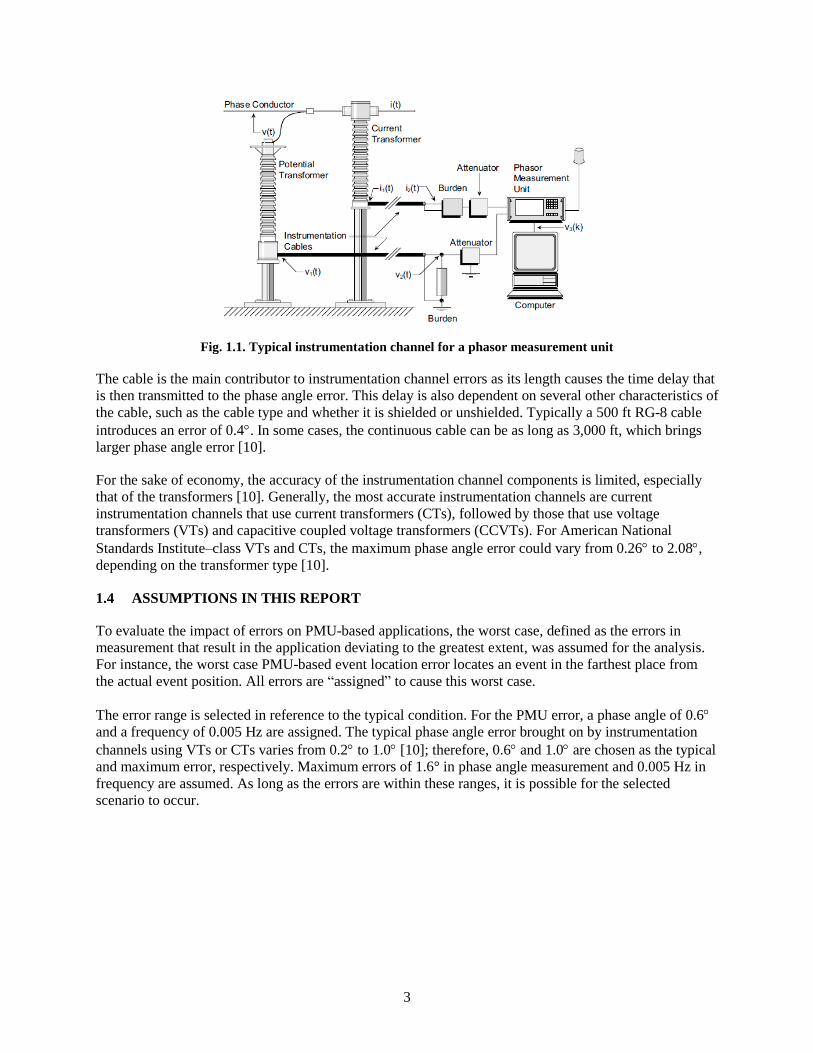
attenuators, as shown in Fig. 1.1 [9].
3
Fig. 1.1. Typical instrumentation channel for a phasor measurement unit
The cable is the main contributor to instrumentation channel errors as its length causes the time delay that
is then transmitted to the phase angle error. This delay is also dependent on several other characteristics of
the cable, such as the cable type and whether it is shielded or unshielded. Typically a 500 ft RG-8 cable
introduces an error of 0.4. In some cases, the continuous cable can be as long as 3,000 ft, which brings
larger phase angle error [10].
For the sake of economy, the accuracy of the instrumentation channel components is limited, especially
that of the transformers [10]. Generally, the most accurate instrumentation channels are current
instrumentation channels that use current transformers (CTs), followed by those that use voltage
transformers (VTs) and capacitive coupled voltage transformers (CCVTs). For American National
Standards Institute–class VTs and CTs, the maximum phase angle error could vary from 0.26 to 2.08,
depending on the transformer type [10].
1.4 ASSUMPTIONS IN THIS REPORT
To evaluate the impact of errors on PMU-based applications, the worst case, defined as the errors in
measurement that result in the application deviating to the greatest extent, was assumed for the analysis.
For instance, the worst case PMU-based event location error locates an event in the farthest place from
the actual event position. All errors are “assigned” to cause this worst case.
The error range is selected in reference to the typical condition. For the PMU error, a phase angle of 0.6
and a frequency of 0.005 Hz are assigned. The typical phase angle error brought on by instrumentation
channels using VTs or CTs varies from 0.2 to 1.0 [10]; therefore, 0.6 and 1.0 are chosen as the typical
and maximum error, respectively. Maximum errors of 1.6° in phase angle measurement and 0.005 Hz in
frequency are assumed. As long as the errors are within these ranges, it is possible for the selected
scenario to occur.

5
2. IMPACT ON EVENT LOCATION
One application of PMUs is detecting and locating disturbance events within a power grid. The method
for this is based on the geometrical triangulation algorithm using the time difference of arrival (TDOA).
A disturbance in the power system, such as generator trip or load shedding, causes frequency and phase
angle variations that propagate along the power network with finite and constant speeds [11]. Using this
principle, it is possible to estimate the location of the disturbance [12]. This application is used by the
power system Frequency Monitoring Network (FNET) [13]. When a disturbance occurs, changes over a
preset threshold will be detected by frequency disturbance recorders (FDRs) on the distribution lines and
transmitted to the FNET server. The server will detect the event and determine its arrival time at different
FDRs. The triangulation algorithm is then used to estimate the location within a circle around the first
responding FDR as it is the nearest one to the event location. Every suspected power plant and pumped
hydroelectric storage unit within this circle is then validated by a linear regression with the data from the
first six responding FDRs. The event plant should give the least fitting residues [1]. Because the
algorithm is based on the phase angle measured from the power grid, measurement error may cause the
event location to be inaccurate or fail altogether. This section presents a study designed to analyze the
level of angle error that will cause event location failure.
2.1 APPROACH
Because the event location is estimated within a circle around the first responding PMU/FDR, the location
triangulation will definitely fail if the first responding device is impacted by error and the real location is
beyond the circle. As the triangulation algorithm uses relative angle values to detect the first responding
unit, we assumed that the impact of instrumentation channel error would be negligible in this case. That is
because all measurement data go through the same channel and contain consistent angle shifts that can be
eliminated during the process of relative angle value calculation. We assumed that, for every single PMU,
the portion of measurement error that impacts the event location application is randomly distributed in the
whole process of measurement within a reasonable band. Based on IEEE Std. C37.118.1-2011 [8], ±0.6
was taken as the maximum PMU measurement error band. Plots of the angle curves are presented
throughout this discussion. The units are seconds for the time and degrees for the angles.
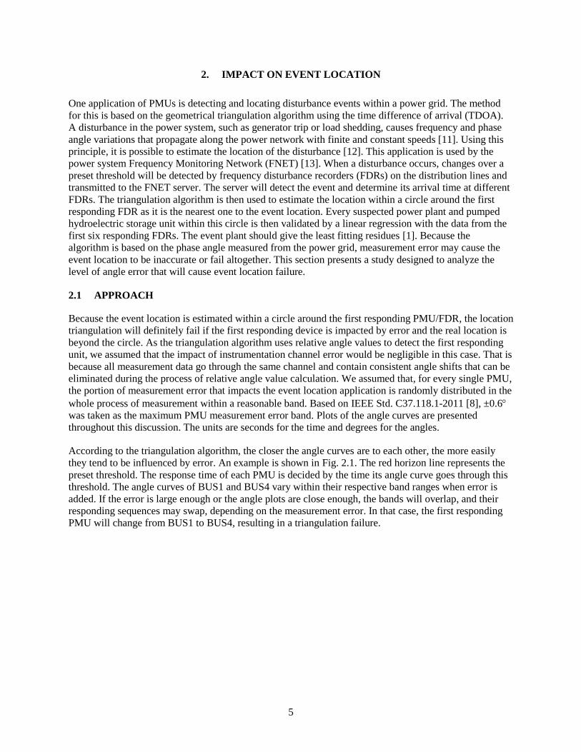
According to the triangulation algorithm, the closer the angle curves are to each other, the more easily
they tend to be influenced by error. An example is shown in Fig. 2.1. The red horizon line represents the
preset threshold. The response time of each PMU is decided by the time its angle curve goes through this
threshold. The angle curves of BUS1 and BUS4 vary within their respective band ranges when error is
added. If the error is large enough or the angle plots are close enough, the bands will overlap, and their
responding sequences may swap, depending on the measurement error. In that case, the first responding
PMU will change from BUS1 to BUS4, resulting in a triangulation failure.
6
Fig. 2.1. Angle curves with error band.
Within the error band, the theoretical PMU measurement error should randomly distribute. To statistically
determine the situations in which the triangulation results would definitely fail would cost much time and
most of the answers might be negative. Assuming the worst case occurs when each PMU measurement
contains the maximum error, either +0.6 or −0.6, there are hundreds of “first six responding unit”
sequences for one event, which may or may not result in different event location results. It depends on the
geographical and electrical relationships between the true event location and the topology of the PMUs.
For the sake of efficiency, different events were tested with several combinations of responding PMU
sequences to verify the existence of PMU measurement error impacts. This report focuses on the cases
that verify the PMU measurement error significantly impacts the event location results.
To demonstrate how the angle error of the PMU impacts event location, angle error is added to different
cases, and the triangulation results before and after the error are added and compared. The study is first
implemented on a Northeast Power Coordinating Council (NPCC) model-based simulation and then on
real power disturbance events. In the first simulation, one generator in the NPCC model is manually
tripped and data from each bus are obtained using the Siemens Power System Simulator for Engineering
(PSS/E). The latter case uses a real event and the related phase angles recorded by FNET.
The main parameters of the algorithm include the event detection threshold, which indicates how much
phase angle change is considered an event, and the search radius, which defines the scale of the circle
centering the first responding device and supposing to compromise the event location. Both parameters
use empirical values. According to [1], 3.2 is used as the threshold of phase angle variation and
200 miles as the circle radius.
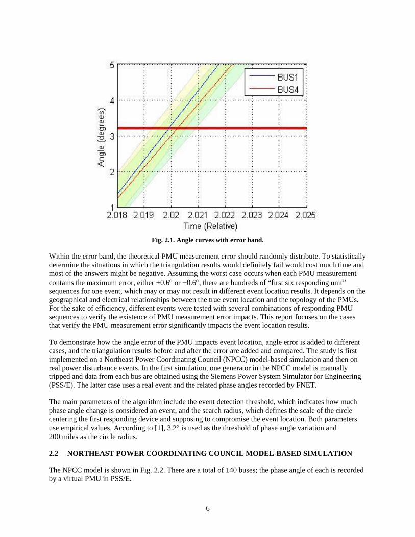
2.2 NORTHEAST POWER COORDINATING COUNCIL MODEL-BASED SIMULATION
The NPCC model is shown in Fig. 2.2. There are a total of 140 buses; the phase angle of each is recorded
by a virtual PMU in PSS/E.
7
Fig. 2.2. Northeast Power Coordinating Council model. (Acronyms used in the figure, such as “PJM” and “NYISO,”
are the names of or stand for regional transmission
organizations.)
In the simulation, generator 1 on Bus 21 is tripped down. All PMUs on other buses respond to this event;
angles of the first six units are plotted in Fig. 2.3. It is noted from the figure that the first responding PMU
is on Bus 1, which is actually the nearest one to Bus 21.
8
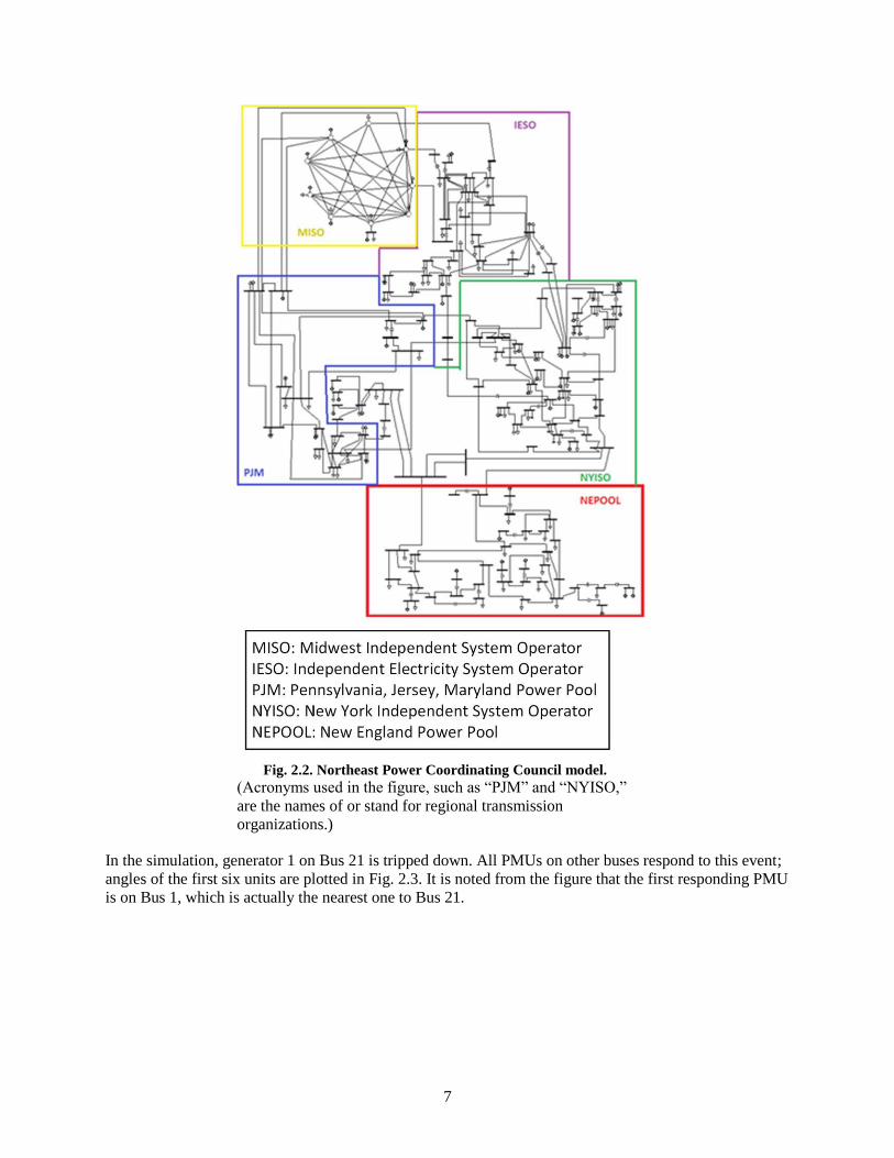
Fig. 2.3. Angle curves of the first six buses. The red horizon line represents the
preset threshold.
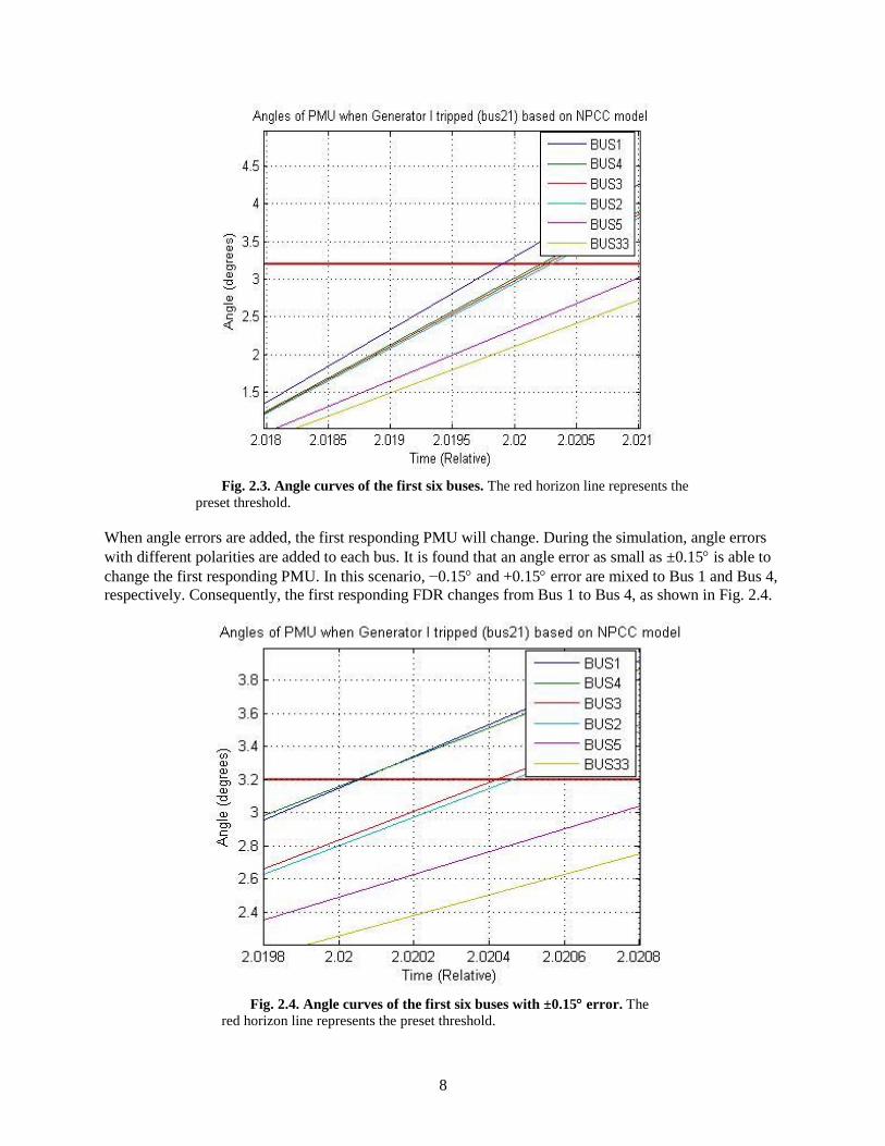
When angle errors are added, the first responding PMU will change. During the simulation, angle errors
with different polarities are added to each bus. It is found that an angle error as small as ±0.15 is able to
change the first responding PMU. In this scenario, −0.15 and +0.15 error are mixed to Bus 1 and Bus 4,
respectively. Consequently, the first responding FDR changes from Bus 1 to Bus 4, as shown in Fig. 2.4.
Fig. 2.4. Angle curves of the first six buses with ±0.15 error. The
red horizon line represents the preset threshold.
9
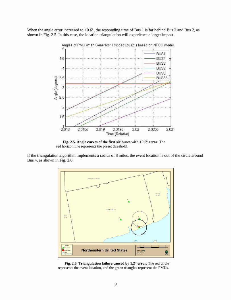
When the angle error increased to ±0.6, the responding time of Bus 1 is far behind Bus 3 and Bus 2, as
shown in Fig. 2.5. In this case, the location triangulation will experience a larger impact.
Fig. 2.5. Angle curves of the first six buses with ±0.6 error. The
red horizon line represents the preset threshold.
If the triangulation algorithm implements a radius of 8 miles, the event location is out of the circle around
Bus 4, as shown in Fig. 2.6.
Fig. 2.6. Triangulation failure caused by 1.2 error. The red circle
represents the event location, and the green triangles represent the PMUs.
10
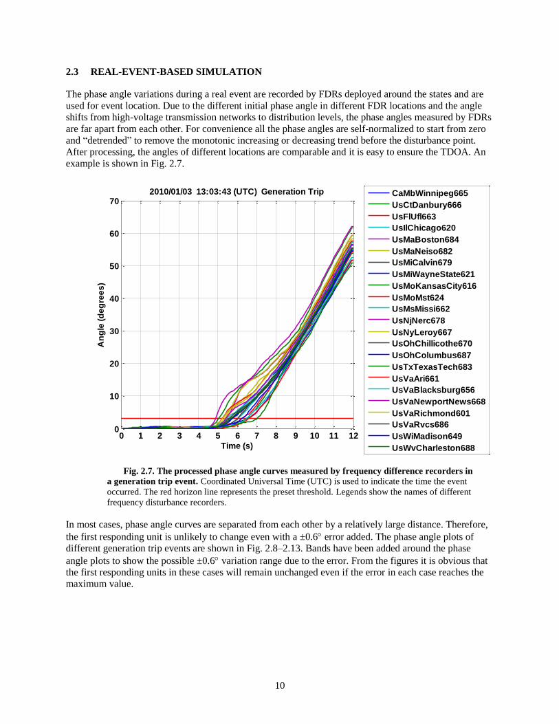
2.3 REAL-EVENT-BASED SIMULATION
The phase angle variations during a real event are recorded by FDRs deployed around the states and are
used for event location. Due to the different initial phase angle in different FDR locations and the angle
shifts from high-voltage transmission networks to distribution levels, the phase angles measured by FDRs
are far apart from each other. For convenience all the phase angles are self-normalized to start from zero
and “detrended” to remove the monotonic increasing or decreasing trend before the disturbance point.
After processing, the angles of different locations are comparable and it is easy to ensure the TDOA. An
example is shown in Fig. 2.7.
Fig. 2.7. The processed phase angle curves measured by frequency difference recorders in
a generation trip event. Coordinated Universal Time (UTC) is used to indicate the time the event
occurred. The red horizon line represents the preset threshold. Legends show the names of different
frequency disturbance recorders.
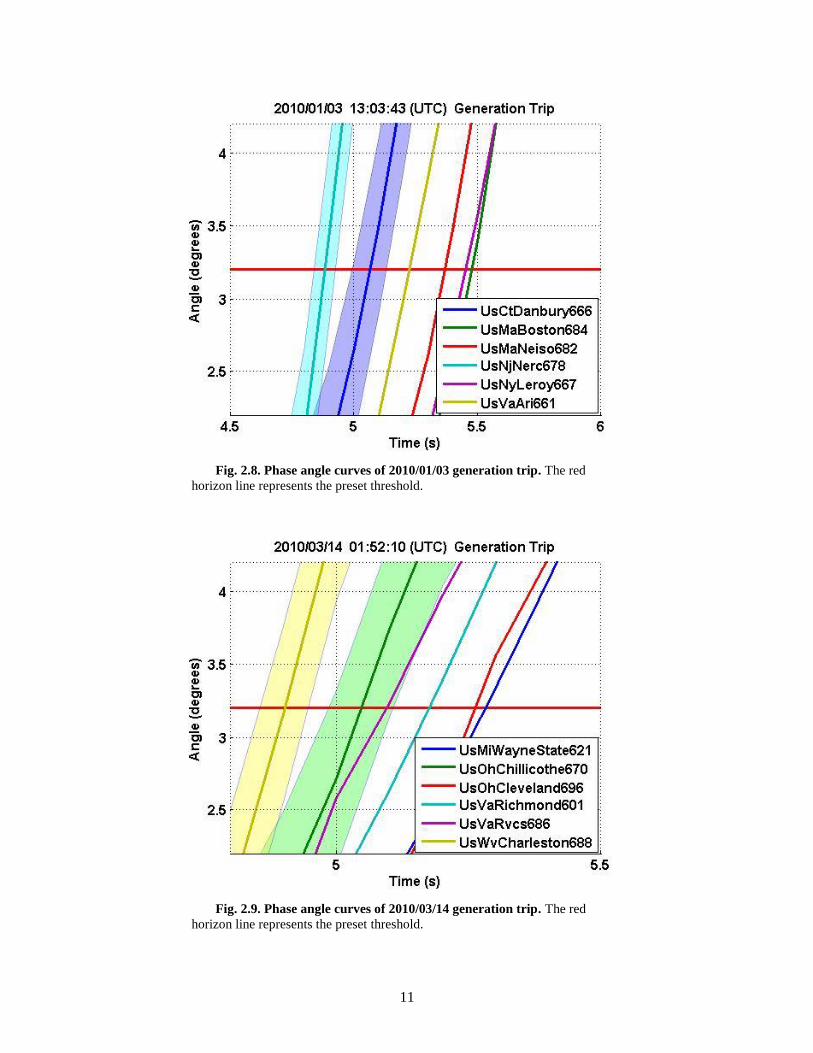
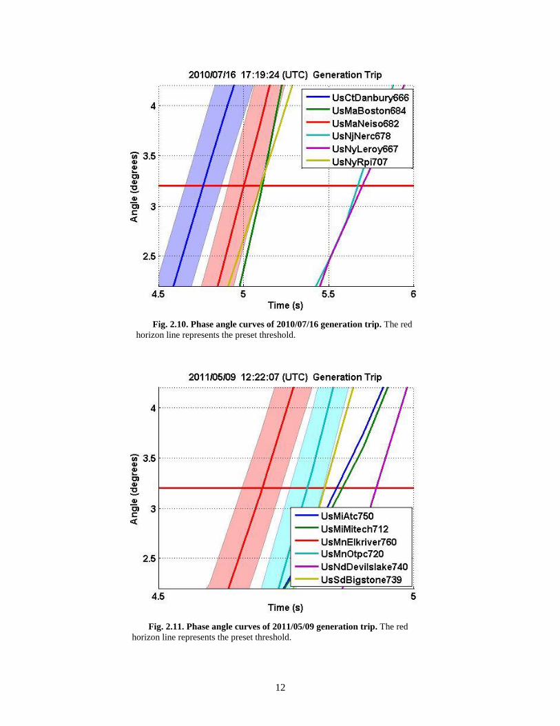
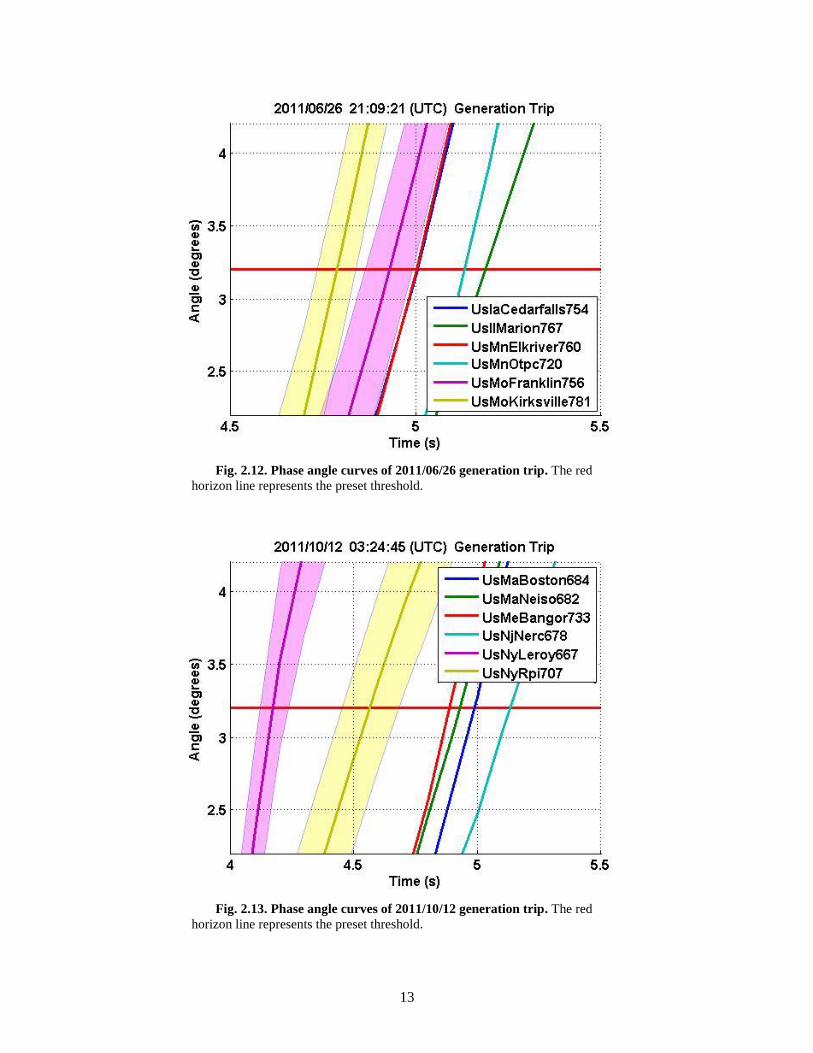
In most cases, phase angle curves are separated from each other by a relatively large distance. Therefore,
the first responding unit is unlikely to change even with a ±0.6 error added. The phase angle plots of
different generation trip events are shown in Fig. 2.8–2.13. Bands have been added around the phase
angle plots to show the possible ±0.6 variation range due to the error. From the figures it is obvious that
the first responding units in these cases will remain unchanged even if the error in each case reaches the
maximum value.
Time (s)
An
gle
(d
eg
ree
s)
2010/01/03 13:03:43 (UTC) Generation Trip
0 1 2 3 4 5 6 7 8 9 10 11 120
10
20
30
40
50
60
70CaMbWinnipeg665
UsCtDanbury666
UsFlUfl663
UsIlChicago620
UsMaBoston684
UsMaNeiso682
UsMiCalvin679
UsMiWayneState621
UsMoKansasCity616
UsMoMst624
UsMsMissi662
UsNjNerc678
UsNyLeroy667
UsOhChillicothe670
UsOhColumbus687
UsTxTexasTech683
UsVaAri661
UsVaBlacksburg656
UsVaNewportNews668
UsVaRichmond601
UsVaRvcs686
UsWiMadison649
UsWvCharleston688
11
Fig. 2.8. Phase angle curves of 2010/01/03 generation trip. The red
horizon line represents the preset threshold.
Fig. 2.9. Phase angle curves of 2010/03/14 generation trip. The red
horizon line represents the preset threshold.
12
Fig. 2.10. Phase angle curves of 2010/07/16 generation trip. The red
horizon line represents the preset threshold.
Fig. 2.11. Phase angle curves of 2011/05/09 generation trip. The red
horizon line represents the preset threshold.
13
Fig. 2.12. Phase angle curves of 2011/06/26 generation trip. The red
horizon line represents the preset threshold.
Fig. 2.13. Phase angle curves of 2011/10/12 generation trip. The red
horizon line represents the preset threshold.
14
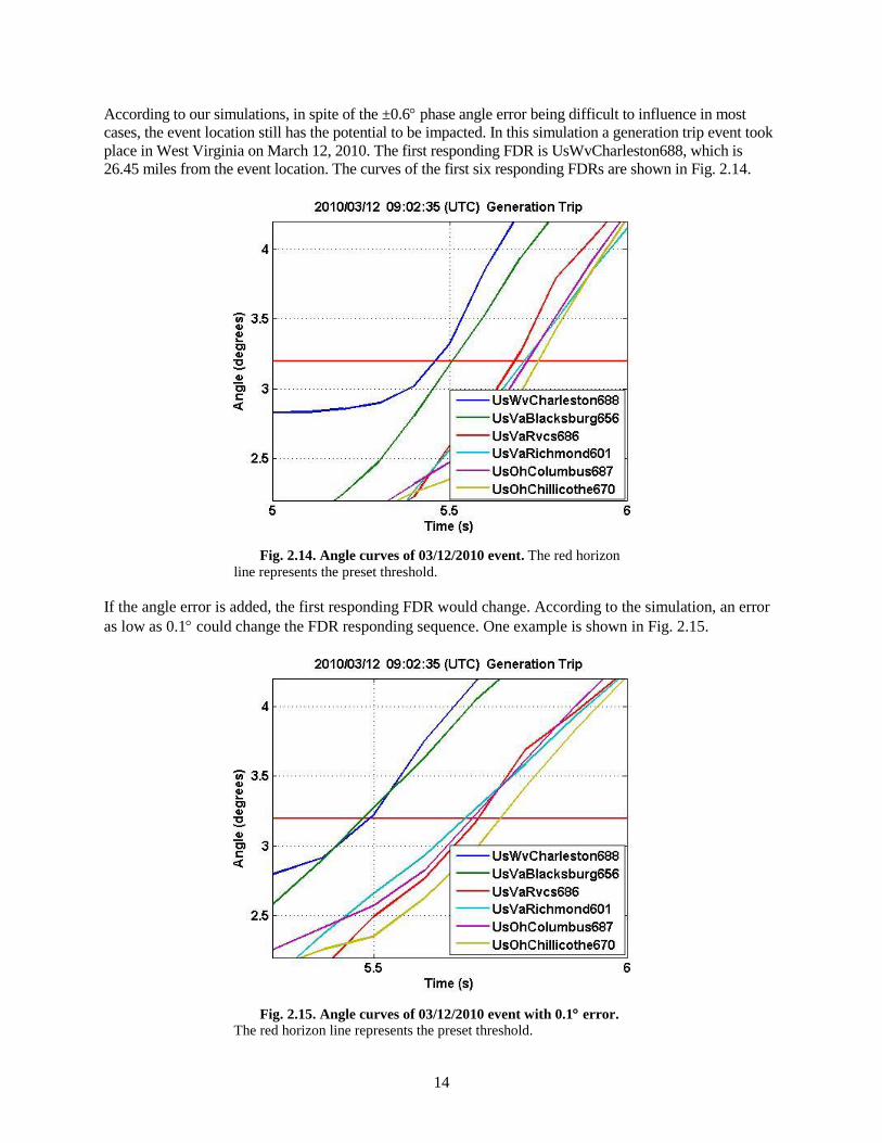
According to our simulations, in spite of the ±0.6 phase angle error being difficult to influence in most
cases, the event location still has the potential to be impacted. In this simulation a generation trip event took
place in West Virginia on March 12, 2010. The first responding FDR is UsWvCharleston688, which is
26.45 miles from the event location. The curves of the first six responding FDRs are shown in Fig. 2.14.
Fig. 2.14. Angle curves of 03/12/2010 event. The red horizon
line represents the preset threshold.
If the angle error is added, the first responding FDR would change. According to the simulation, an error
as low as 0.1 could change the FDR responding sequence. One example is shown in Fig. 2.15.
Fig. 2.15. Angle curves of 03/12/2010 event with 0.1 error. The red horizon line represents the preset threshold.
15
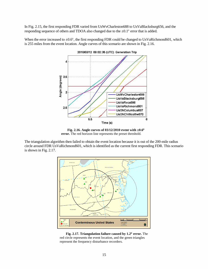
In Fig. 2.15, the first responding FDR varied from UsWvCharleston688 to UsVaBlacksburg656, and the
responding sequence of others and TDOA also changed due to the ±0.1 error that is added.
When the error increased to ±0.6, the first responding FDR could be changed to UsVaRichmond601, which
is 255 miles from the event location. Angle curves of this scenario are shown in Fig. 2.16.
Fig. 2.16. Angle curves of 03/12/2010 event with ±0.6 error. The red horizon line represents the preset threshold.
The triangulation algorithm then failed to obtain the event location because it is out of the 200-mile radius
circle around FDR UsVaRichmond601, which is identified as the current first responding FDR. This scenario
is shown in Fig. 2.17.
Fig. 2.17. Triangulation failure caused by 1.2 error. The
red circle represents the event location, and the green triangles
represent the frequency disturbance recorders.

16
2.4 SUMMARY OF EVENT LOCATION IMPACT
Angle-based event location is a PMU-based application that uses the phase angle of the power grid to
detect and locate the disturbance event. The angle error in most cases does not impact the accuracy of the
triangulation algorithm. However, in some cases the angle error is able to cause triangulation failure.
Basically, the first responding PMU is the unit most vulnerable to the angle error. According to the cases
analyzed above, angle error as low as ±0.1 can cause a failure, and an angle error of ±0.6 will have an
even greater impact.
17
3. IMPACT ON OSCILLATION DETECTION
Small signal stability problems with the power grid can potentially cause significant electromechanical
oscillations, which may lead to grid reliability issues and potentially large-scale blackouts. PMUs provide
high-precision time-synchronized data for oscillation detection. Frequency and phase angle measured by a
PMU can be used for oscillation detection. However, the measurement error will affect the detection
result, even resulting in its failure. In this section, the phase-angle-based oscillation detection is described
first, and the impact of measurement error is analyzed.
3.1 APPROACH
Currently, angle measurement from PMUs, instead of frequency measurement, is used for oscillation
detection, mainly because angle measurement has a lower signal-to-noise ratio (SNR). Because the phase
angle deviation in PMU measurement is the integral of the frequency measurement deviation, an
oscillation of small amplitude in frequency can cause the angle to obtain a much higher SNR [2].
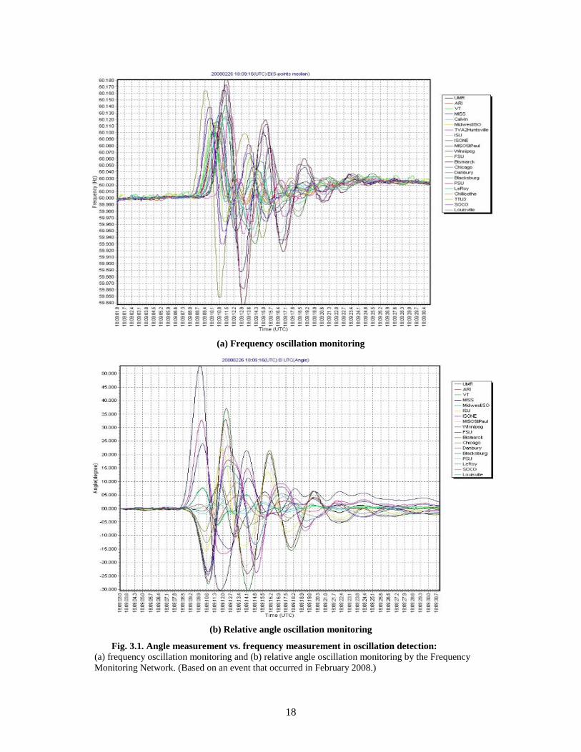
Figure 3.1 shows an obvious oscillation that happened in February 2008. As shown, system frequency
extends from 59.84 to 60.18 Hz, with a total deviation of about 0.34 Hz. However, the relative phase
angle extends from −30 to 55 during the same event, with a total angle deviation of nearly 85. The
resolution obtained from the angle deviation during this oscillation event is much higher than that from
the frequency measurement.
The oscillation detection module monitors the incoming phasor data in parallel with the frequency event
detection module. The difference is that the oscillation detection module will use the angle data instead of
the frequency. To obtain the relative angle deviations, the absolute angle measurements from PMUs are
processed by referring to a reference PMU and then the angle value of each PMU is normalized to start
from zero by subtracting the angle from the starting angle point of each PMU measurement.
The relative angle remains stable without much deviation when the system is operating in a steady state,
though it changes abruptly during events because of the power angle redistribution associated with the
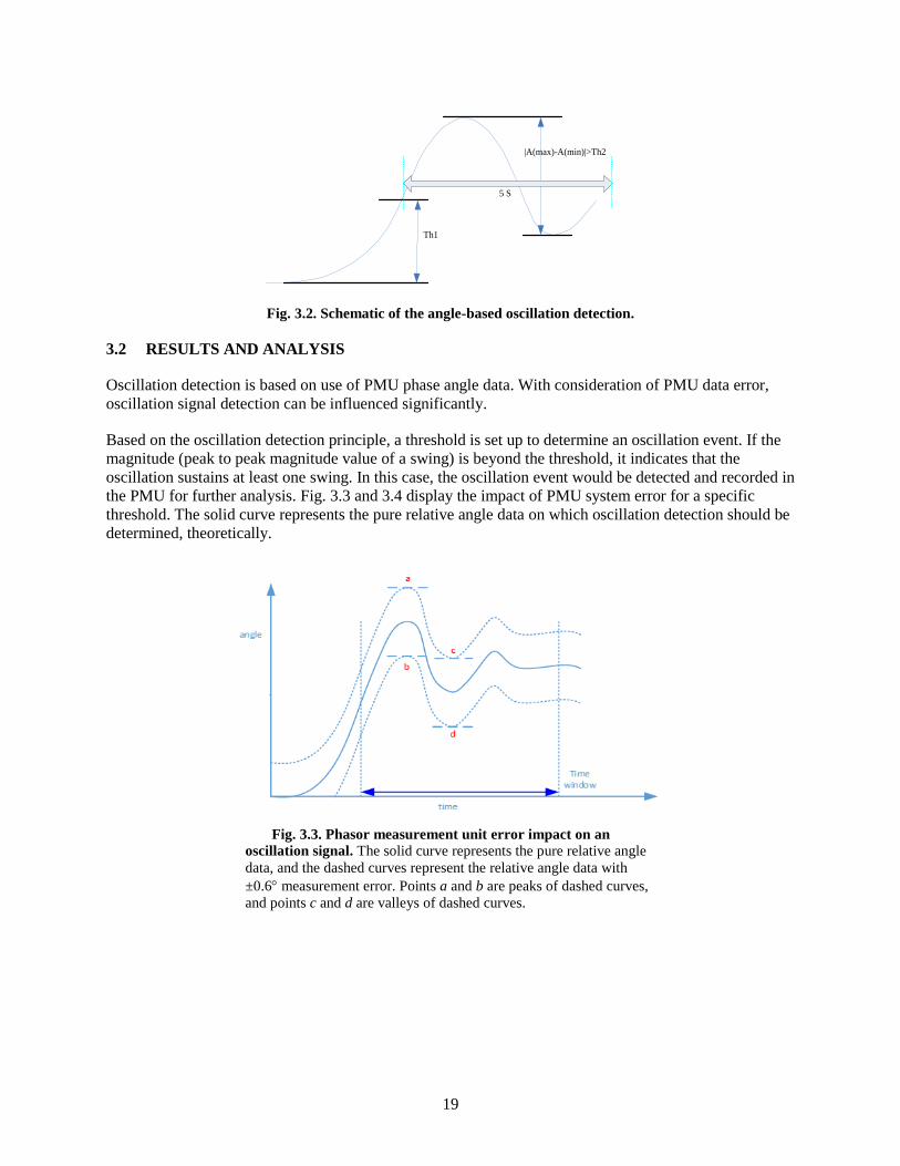
event. The relative angles will form a wavy curve during the oscillation. The signature of an event will
usually show an oscillation data pattern that has a steep angle rise or drop beyond a certain threshold right
after disturbances and then, following the oscillation starting point, the oscillation magnitude (the peak-
peak magnitude of a swing) goes beyond a certain limit and the oscillation is sustained for at least one
swing. The schematic diagram for this is shown in Fig. 3.2. Here the 5-second span is an empirical value
derived from the fact that the frequency of the inter-area oscillation normally ranges from 0.1 Hz to
1.0 Hz.
Oscillation detection uses the same relative angle values as the event location application. The impact on
oscillation detection results is brought about primarily by the random error from the PMU, but the impact
of instrumentation channel error can be neutralized. Likewise, the maximum PMU measurement error
band is considered as ±0.6 based on IEEE Std. C37.118.1-2011.
18
(a) Frequency oscillation monitoring
(b) Relative angle oscillation monitoring
Fig. 3.1. Angle measurement vs. frequency measurement in oscillation detection: (a) frequency oscillation monitoring and (b) relative angle oscillation monitoring by the Frequency
Monitoring Network. (Based on an event that occurred in February 2008.)
19
Th1
|A(max)-A(min)|>Th2
5 S
Fig. 3.2. Schematic of the angle-based oscillation detection.
3.2 RESULTS AND ANALYSIS
Oscillation detection is based on use of PMU phase angle data. With consideration of PMU data error,
oscillation signal detection can be influenced significantly.
Based on the oscillation detection principle, a threshold is set up to determine an oscillation event. If the
magnitude (peak to peak magnitude value of a swing) is beyond the threshold, it indicates that the
oscillation sustains at least one swing. In this case, the oscillation event would be detected and recorded in
the PMU for further analysis. Fig. 3.3 and 3.4 display the impact of PMU system error for a specific
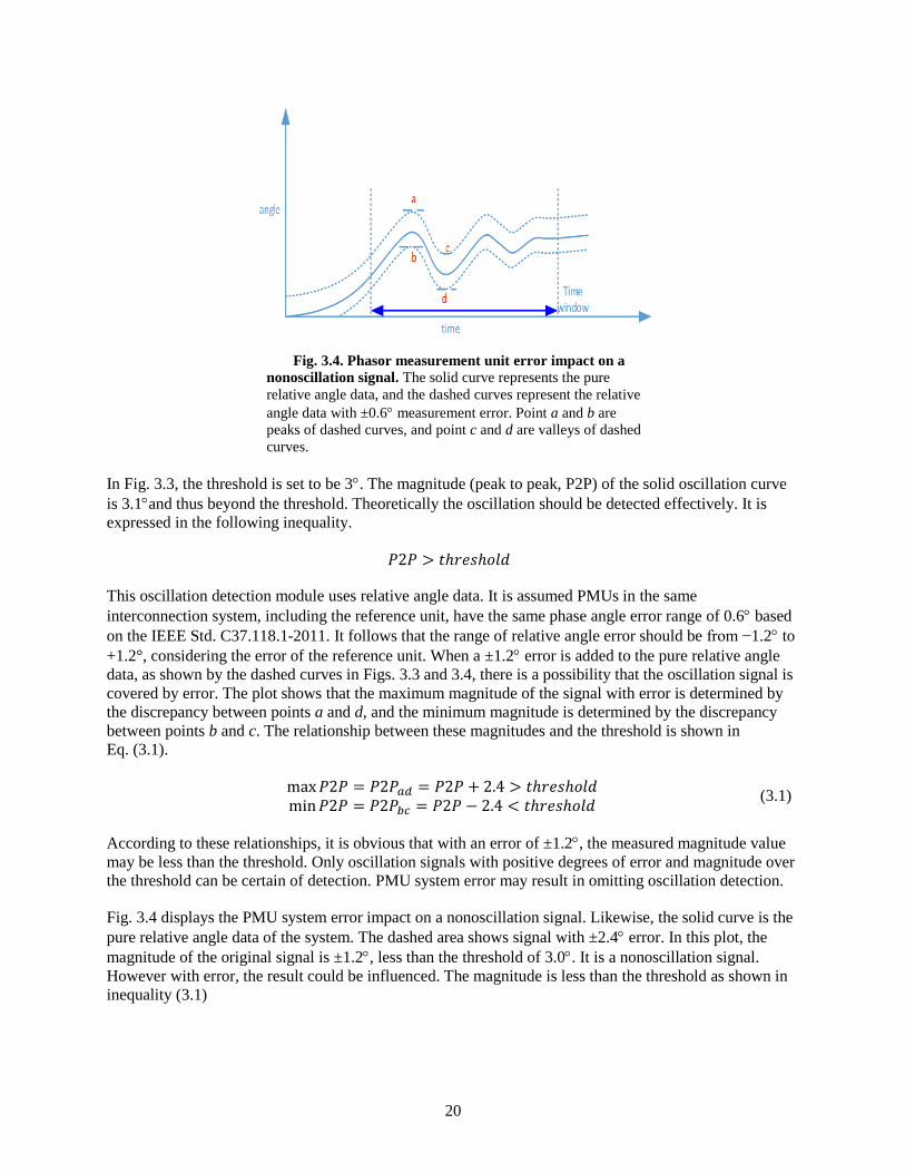
threshold. The solid curve represents the pure relative angle data on which oscillation detection should be
determined, theoretically.
Fig. 3.3. Phasor measurement unit error impact on an
oscillation signal. The solid curve represents the pure relative angle
data, and the dashed curves represent the relative angle data with
±0.6 measurement error. Points a and b are peaks of dashed curves,
and points c and d are valleys of dashed curves.
20
Fig. 3.4. Phasor measurement unit error impact on a
nonoscillation signal. The solid curve represents the pure
relative angle data, and the dashed curves represent the relative
angle data with ±0.6 measurement error. Point a and b are
peaks of dashed curves, and point c and d are valleys of dashed
curves.
In Fig. 3.3, the threshold is set to be 3. The magnitude (peak to peak, P2P) of the solid oscillation curve
is 3.1and thus beyond the threshold. Theoretically the oscillation should be detected effectively. It is
expressed in the following inequality.
𝑃2𝑃 > 𝑡ℎ𝑟𝑒𝑠ℎ𝑜𝑙𝑑
This oscillation detection module uses relative angle data. It is assumed PMUs in the same
interconnection system, including the reference unit, have the same phase angle error range of 0.6 based
on the IEEE Std. C37.118.1-2011. It follows that the range of relative angle error should be from −1.2 to
+1.2°, considering the error of the reference unit. When a ±1.2 error is added to the pure relative angle
data, as shown by the dashed curves in Figs. 3.3 and 3.4, there is a possibility that the oscillation signal is
covered by error. The plot shows that the maximum magnitude of the signal with error is determined by
the discrepancy between points a and d, and the minimum magnitude is determined by the discrepancy
between points b and c. The relationship between these magnitudes and the threshold is shown in
Eq. (3.1).
max 𝑃2𝑃 = 𝑃2𝑃𝑎𝑑 = 𝑃2𝑃 + 2.4 > 𝑡ℎ𝑟𝑒𝑠ℎ𝑜𝑙𝑑
min 𝑃2𝑃 = 𝑃2𝑃𝑏𝑐 = 𝑃2𝑃 − 2.4 < 𝑡ℎ𝑟𝑒𝑠ℎ𝑜𝑙𝑑 (3.1)
According to these relationships, it is obvious that with an error of ±1.2, the measured magnitude value
may be less than the threshold. Only oscillation signals with positive degrees of error and magnitude over
the threshold can be certain of detection. PMU system error may result in omitting oscillation detection.
Fig. 3.4 displays the PMU system error impact on a nonoscillation signal. Likewise, the solid curve is the
pure relative angle data of the system. The dashed area shows signal with ±2.4 error. In this plot, the
magnitude of the original signal is ±1.2, less than the threshold of 3.0. It is a nonoscillation signal.
However with error, the result could be influenced. The magnitude is less than the threshold as shown in
inequality (3.1)
21
As shown in Fig. 3.4, it is highly possible that the magnitude is changed to be the deviation between
points a and d, the original magnitude with positive 2.4 error. Finally, the magnitude is changed to be
4.8, beyond the threshold of 3.0. This relationship is shown in Eq. (3.2).
max 𝑃2𝑃 = 𝑃2𝑃𝑎𝑑 = 𝑃2𝑃 + 2.4 > 𝑡ℎ𝑟𝑒𝑠ℎ𝑜𝑙𝑑 (3.2)
In this case, the nonoscillation signal is detected as an oscillation. Apparently this incorrect detection is
influenced by the PMU system error.
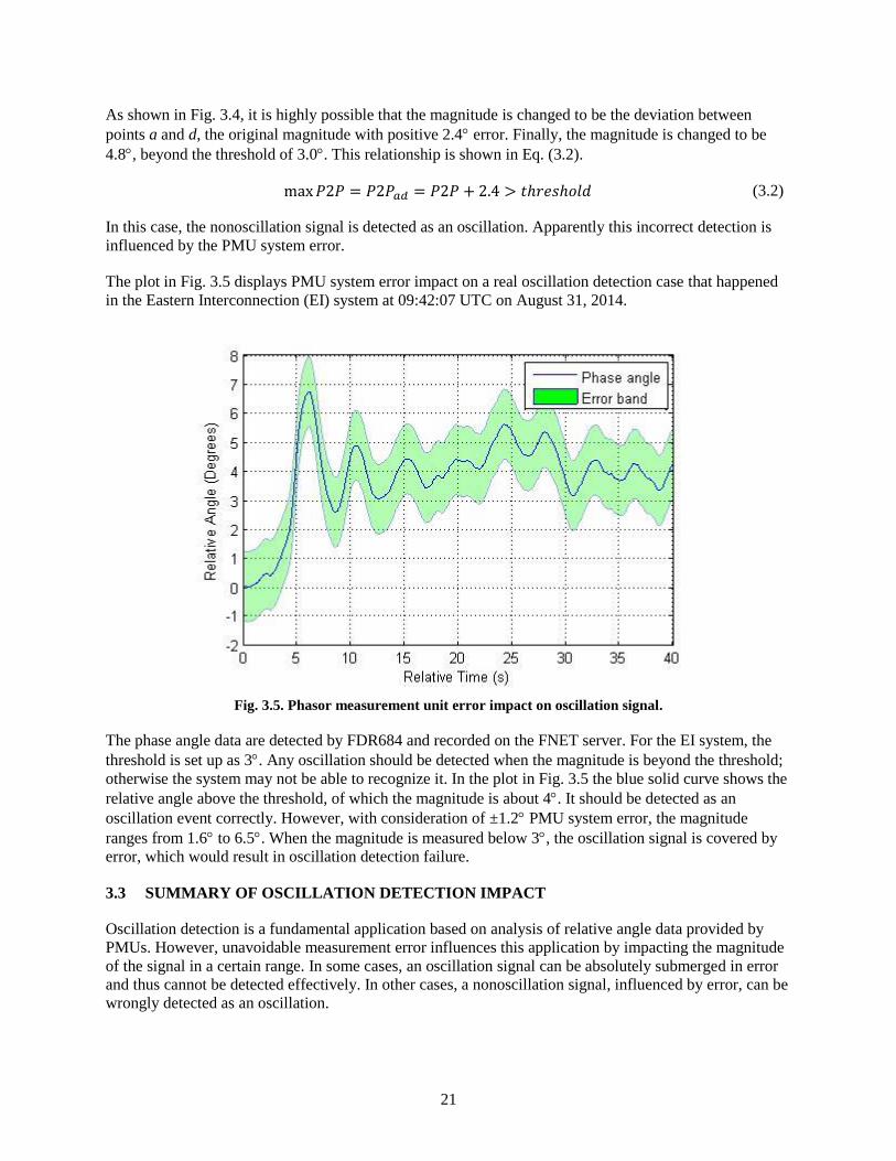
The plot in Fig. 3.5 displays PMU system error impact on a real oscillation detection case that happened
in the Eastern Interconnection (EI) system at 09:42:07 UTC on August 31, 2014.
Fig. 3.5. Phasor measurement unit error impact on oscillation signal.
The phase angle data are detected by FDR684 and recorded on the FNET server. For the EI system, the
threshold is set up as 3. Any oscillation should be detected when the magnitude is beyond the threshold;
otherwise the system may not be able to recognize it. In the plot in Fig. 3.5 the blue solid curve shows the
relative angle above the threshold, of which the magnitude is about 4. It should be detected as an
oscillation event correctly. However, with consideration of ±1.2 PMU system error, the magnitude
ranges from 1.6 to 6.5. When the magnitude is measured below 3, the oscillation signal is covered by
error, which would result in oscillation detection failure.
3.3 SUMMARY OF OSCILLATION DETECTION IMPACT
Oscillation detection is a fundamental application based on analysis of relative angle data provided by
PMUs. However, unavoidable measurement error influences this application by impacting the magnitude
of the signal in a certain range. In some cases, an oscillation signal can be absolutely submerged in error
and thus cannot be detected effectively. In other cases, a nonoscillation signal, influenced by error, can be
wrongly detected as an oscillation.

23
4. IMPACT ON ISLANDING DETECTION
DG, which uses fuel cells, micro-hydro, photovoltaics, etc. and is placed close to the load being served, is
a new shift in the power industry to take advantage of economic and eco-friendly energy sources [14].
However many issues are involved with DG. One of the main issues is islanding, the situation where a
distribution system becomes electrically isolated from the remainder of the power system while
continuing to be powered by DG sources. Islanding threatens the safety of line workers and causes the
distribution sources to be out of phase with the utility power supply when reclosing. Therefore it is very
important to detect islanding quickly and accurately.
PMUs can capture the characteristics of frequency and phase angle change during the islanding
generation and could be used for islanding detection. Furthermore, the PMUs network overcomes the
limitation of traditional methods such as small mismatch and topology adaptation. Therefore, the
application of PMUs in islanding detection is essentially promising.
Because frequency and phase angle are used for this application, their errors may influence the detection
precision and results. The islanding detection method studied here is based on the frequency measurement
of FNET [15], and the error impact is demonstrated.
4.1 APPROACH
In this algorithm, frequency deviation (FD) for all the FDRs is calculated by
𝐹𝐷𝑖(𝑡) = |𝑓𝑖(𝑡) − 𝑓ref(𝑡)| , (4.1)
where 𝑓𝑖(𝑡) is the measured frequency value of the ith FDR at timestamp t and 𝑓ref(𝑡) is defined as the
median value of all the monitored FDRs in the same interconnection.
𝑓ref(𝑡) = 𝑚𝑒𝑑𝑖𝑎𝑛(𝑓1(𝑡), 𝑓2(𝑡), … , 𝑓𝑁(𝑡)). (4.2)
The integration of frequency deviation (IOFD) is defined as the accumulation of the FD over a certain
time period, given by
𝐼𝑂𝐹𝐷𝑖 = ∑ 𝐹𝐷𝑖(𝑡)
𝑡2
𝑡=𝑡1
, (4.3)
where t1 and t2 are the start and end times, respectively, for this integration time period. It is used for false
event rejection.
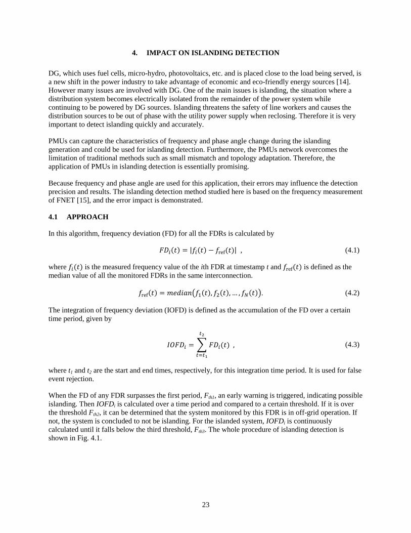
When the FD of any FDR surpasses the first period, Fth1, an early warning is triggered, indicating possible
islanding. Then IOFDi is calculated over a time period and compared to a certain threshold. If it is over
the threshold Fth2, it can be determined that the system monitored by this FDR is in off-grid operation. If
not, the system is concluded to not be islanding. For the islanded system, IOFDi is continuously
calculated until it falls below the third threshold, Fth3. The whole procedure of islanding detection is
shown in Fig. 4.1.
24
Calculate FDi(t)
FDR
Real-time Data
FDi(t)>Fth1
Calculate
IOFDi(t)IOFDi(t)>Fth2
IOFDi(t)<Fth3
Calculate
IOFDi(t)
Fig. 4.1. Flow chart of the islanding detection method.
When the frequency angle is mixed with the measurement error, the result of FDi and IOFDi will also be
influenced. This may cause the islanding detection method to fail or give a false alarm. To demonstrate
this situation, an islanding detection case is selected. Data collected by FDRs are fed into the algorithm to
verify the correction of the method. Frequency error is then manually added to the data and the new
detection result is compared with the original one to identify the impact caused by measurement error.
4.2 RESULTS AND ANALYSIS
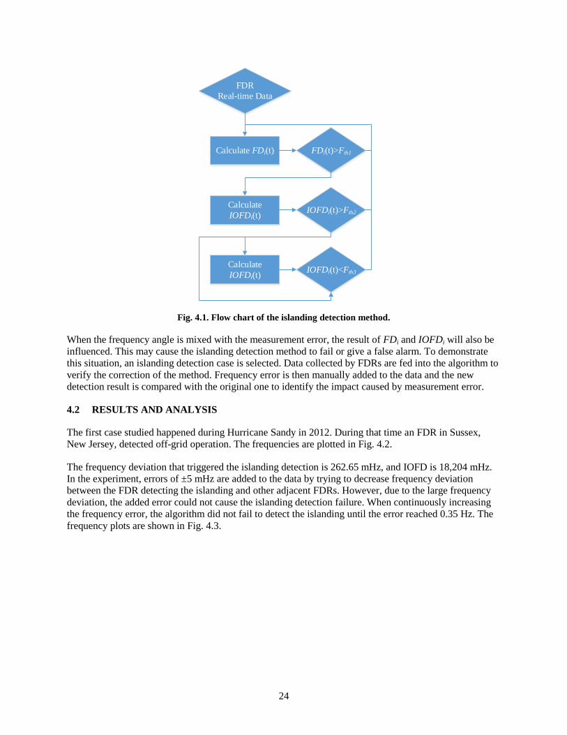
The first case studied happened during Hurricane Sandy in 2012. During that time an FDR in Sussex,
New Jersey, detected off-grid operation. The frequencies are plotted in Fig. 4.2.
The frequency deviation that triggered the islanding detection is 262.65 mHz, and IOFD is 18,204 mHz.
In the experiment, errors of ±5 mHz are added to the data by trying to decrease frequency deviation
between the FDR detecting the islanding and other adjacent FDRs. However, due to the large frequency
deviation, the added error could not cause the islanding detection failure. When continuously increasing
the frequency error, the algorithm did not fail to detect the islanding until the error reached 0.35 Hz. The
frequency plots are shown in Fig. 4.3.
25
Fig. 4.2. Frequency measured by frequency
disturbance recorders in the Hurricane Sandy case.
Fig. 4.3. Frequency with 0.35 Hz error in the Hurricane Sandy case.
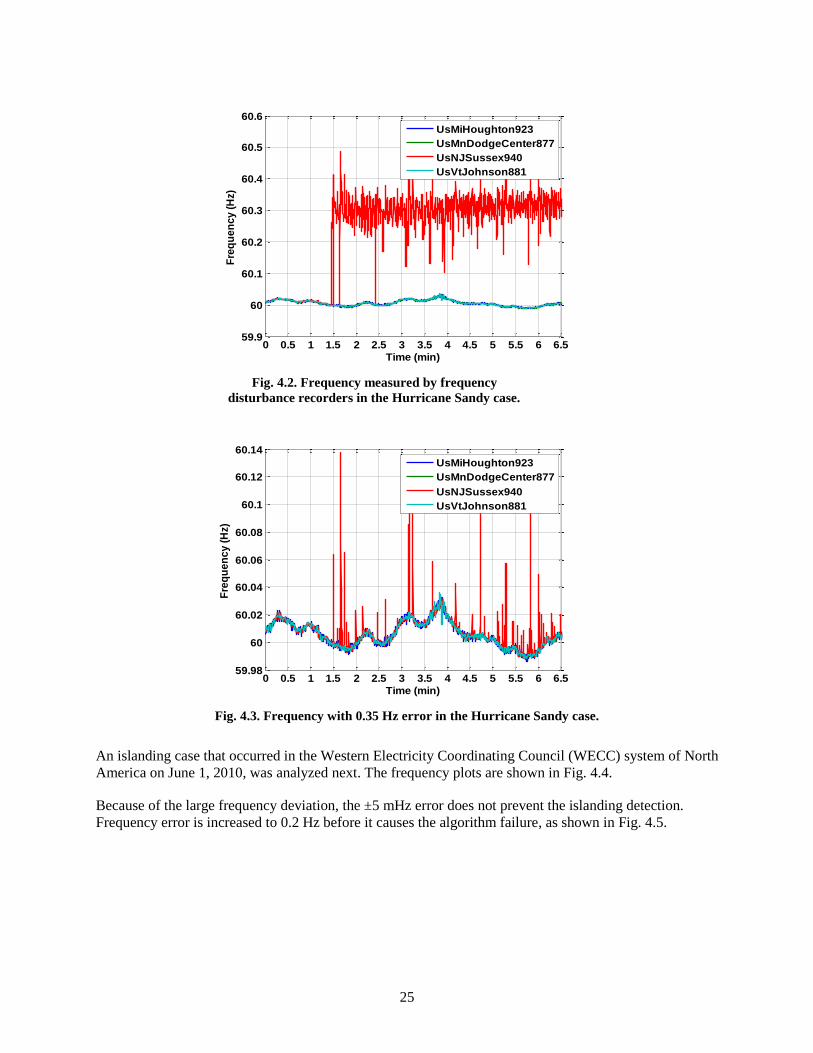
An islanding case that occurred in the Western Electricity Coordinating Council (WECC) system of North
America on June 1, 2010, was analyzed next. The frequency plots are shown in Fig. 4.4.
Because of the large frequency deviation, the ±5 mHz error does not prevent the islanding detection.
Frequency error is increased to 0.2 Hz before it causes the algorithm failure, as shown in Fig. 4.5.
0 0.5 1 1.5 2 2.5 3 3.5 4 4.5 5 5.5 6 6.559.9
60
60.1
60.2
60.3
60.4
60.5
60.6
Time (min)
Fre
qu
en
cy
(H
z)
UsMiHoughton923
UsMnDodgeCenter877
UsNJSussex940
UsVtJohnson881
0 0.5 1 1.5 2 2.5 3 3.5 4 4.5 5 5.5 6 6.559.98
60
60.02
60.04
60.06
60.08
60.1
60.12
60.14
Time (min)
Fre
qu
en
cy
(H
z)
UsMiHoughton923
UsMnDodgeCenter877
UsNJSussex940
UsVtJohnson881
26
Fig. 4.4. Frequencies measured by frequency
disturbance recorders in the 2010/06/01 Western Electricity
Coordinating Council islanding case.
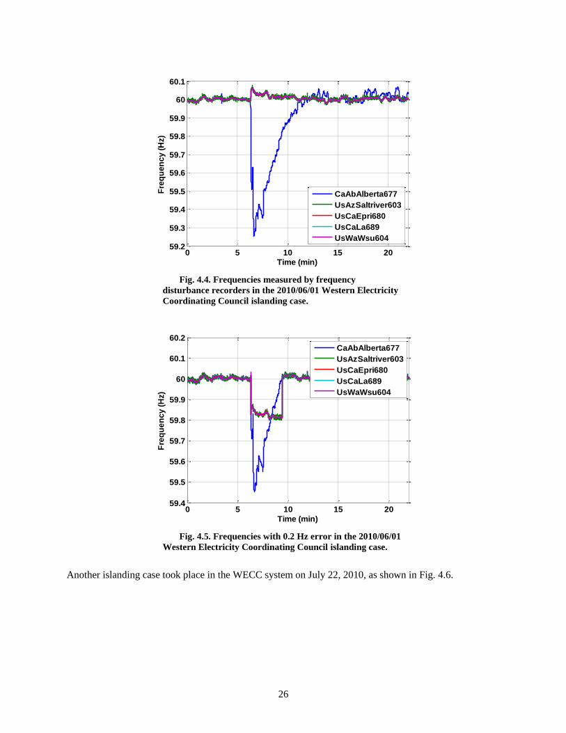
Fig. 4.5. Frequencies with 0.2 Hz error in the 2010/06/01
Western Electricity Coordinating Council islanding case.
Another islanding case took place in the WECC system on July 22, 2010, as shown in Fig. 4.6.
0 5 10 15 2059.2
59.3
59.4
59.5
59.6
59.7
59.8
59.9
60
60.1
Time (min)
Fre
qu
en
cy
(H
z)
CaAbAlberta677
UsAzSaltriver603
UsCaEpri680
UsCaLa689
UsWaWsu604
0 5 10 15 2059.4
59.5
59.6
59.7
59.8
59.9
60
60.1
60.2
Time (min)
Fre
qu
en
cy
(H
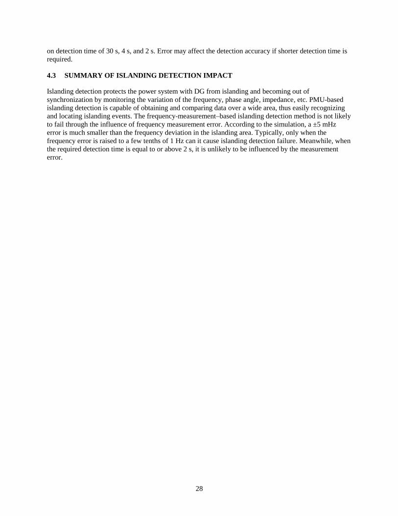
z)
CaAbAlberta677
UsAzSaltriver603
UsCaEpri680
UsCaLa689
UsWaWsu604
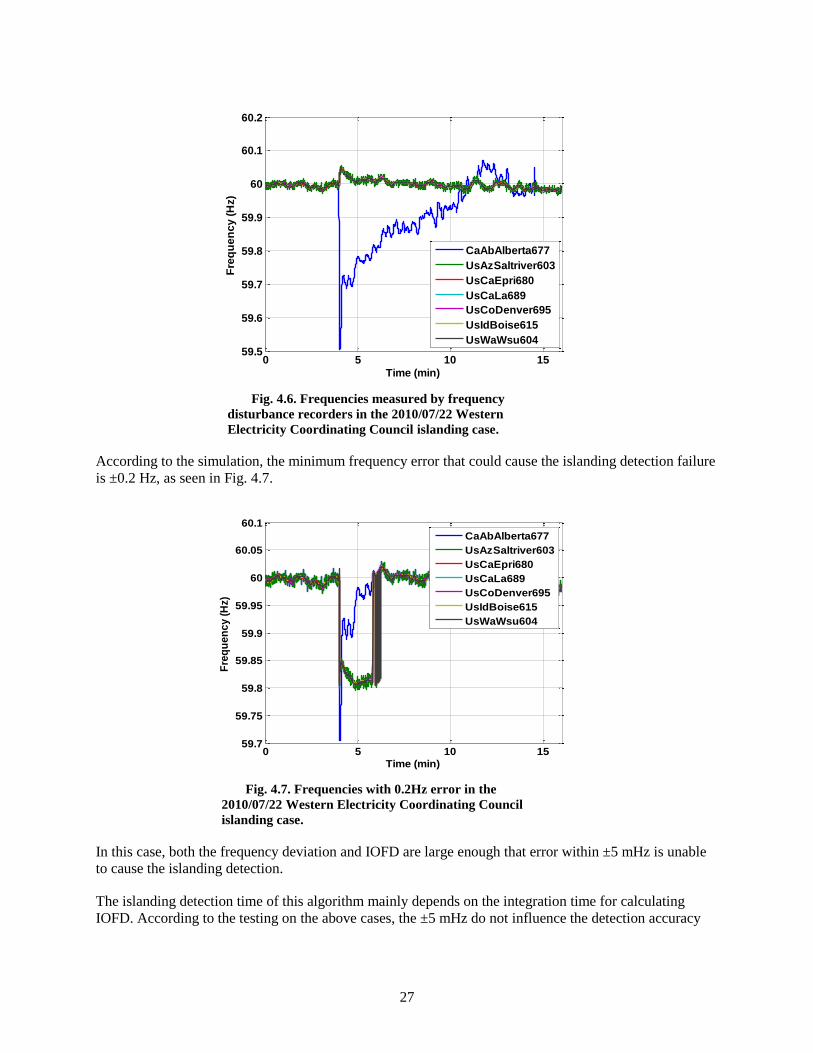
27
Fig. 4.6. Frequencies measured by frequency
disturbance recorders in the 2010/07/22 Western
Electricity Coordinating Council islanding case.
According to the simulation, the minimum frequency error that could cause the islanding detection failure
is ±0.2 Hz, as seen in Fig. 4.7.
Fig. 4.7. Frequencies with 0.2Hz error in the
2010/07/22 Western Electricity Coordinating Council
islanding case.
In this case, both the frequency deviation and IOFD are large enough that error within ±5 mHz is unable
to cause the islanding detection.
The islanding detection time of this algorithm mainly depends on the integration time for calculating
IOFD. According to the testing on the above cases, the ±5 mHz do not influence the detection accuracy
0 5 10 1559.5
59.6
59.7
59.8
59.9
60
60.1
60.2
Time (min)
Fre
qu
en
cy
(H
z)
CaAbAlberta677
UsAzSaltriver603
UsCaEpri680
UsCaLa689
UsCoDenver695
UsIdBoise615
UsWaWsu604
0 5 10 1559.7
59.75
59.8
59.85
59.9
59.95
60
60.05
60.1
Time (min)
Fre
qu
en
cy
(H
z)
CaAbAlberta677
UsAzSaltriver603
UsCaEpri680
UsCaLa689
UsCoDenver695
UsIdBoise615
UsWaWsu604
28
on detection time of 30 s, 4 s, and 2 s. Error may affect the detection accuracy if shorter detection time is
required.
4.3 SUMMARY OF ISLANDING DETECTION IMPACT
Islanding detection protects the power system with DG from islanding and becoming out of
synchronization by monitoring the variation of the frequency, phase angle, impedance, etc. PMU-based
islanding detection is capable of obtaining and comparing data over a wide area, thus easily recognizing
and locating islanding events. The frequency-measurement–based islanding detection method is not likely
to fail through the influence of frequency measurement error. According to the simulation, a ±5 mHz
error is much smaller than the frequency deviation in the islanding area. Typically, only when the
frequency error is raised to a few tenths of 1 Hz can it cause islanding detection failure. Meanwhile, when
the required detection time is equal to or above 2 s, it is unlikely to be influenced by the measurement
error.
29
5. IMPACT ON DYNAMIC LINE RATING
The rating of a transmission line indicates the highest current that the line can transfer safely without
damaging transmission components or jeopardizing the network’s safety, stability, and reliability.
Normally the rating is determined by the maximum conductor temperature or the minimum clearance
from the conductor to the ground [16]. Several factors also affect a line’s rating, such as ambient weather
conditions (temperature, wind speed, solar radiation, etc.), conductor size, and resistance.
Traditionally, static line rating (SLR) is widely used by transmission owners and operators. However,
SLR relies on the worst weather conditions [e.g., high ambient temperature (40℃), low wind speed
(0.61m/s), and full sun] and is considered too conservative [17].
DLR technology is developed to satisfy the increasing transmission capacity and effectively use the actual
capacity of the transmission line. DLR technology monitors the time-varying weather and load
conditions. Communication technologies are used to transfer these data to the DLR algorithm, which
determines the capacity of the transmission line based on the real-time conditions.
5.1 APPROACH
IEEE Standard 738-2012 provides the mathematical equations to define the thermal behavior of the
conductor, which can be used to calculate SLR, transient line rating, and DLR.
Up to now, two main methods have been used for real-time monitoring and DLR calculations. One is
based on the sag monitor of the transmission line [18]. Alternatively, DLR technology uses PMU
measurement data at both ends of the transmission line to calculate DLR [19]. The first method, which
doesn’t use PMU measurement data, is beyond the scope of this report.
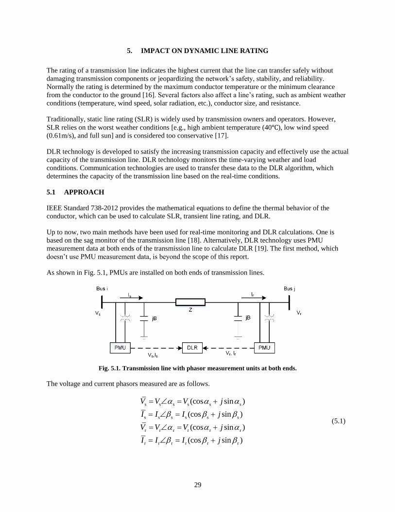
As shown in Fig. 5.1, PMUs are installed on both ends of transmission lines.
Fig. 5.1. Transmission line with phasor measurement units at both ends.
The voltage and current phasors measured are as follows.
s s s s s s
s s s s s s
r r r r r r
r r r r r r
(cos sin )
(cos sin )
(cos sin )
(cos sin )
V V V j
I I I j
V V V j
I I I j
(5.1)
30
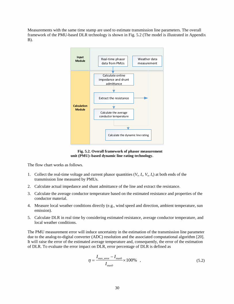
Measurements with the same time stamp are used to estimate transmission line parameters. The overall
framework of the PMU-based DLR technology is shown in Fig. 5.2 (The model is illustrated in Appendix
B).
InputModule
CalculationModule
Calculate online impedance and shunt
admittance
Real-time phasor data from PMUs
Weather data measurement
Extract the resistance
Calculate the average conductor temperature
Calculate the dynamic line rating
Fig. 5.2. Overall framework of phasor measurement
unit (PMU)–based dynamic line rating technology.
The flow chart works as follows.
1. Collect the real-time voltage and current phasor quantities (Vr, Ir, Vs, Is) at both ends of the
transmission line measured by PMUs.
2. Calculate actual impedance and shunt admittance of the line and extract the resistance.
3. Calculate the average conductor temperature based on the estimated resistance and properties of the
conductor material.
4. Measure local weather conditions directly (e.g., wind speed and direction, ambient temperature, sun
emission).
5. Calculate DLR in real time by considering estimated resistance, average conductor temperature, and
local weather conditions.
The PMU measurement error will induce uncertainty in the estimation of the transmission line parameter
due to the analog-to-digital converter (ADC) resolution and the associated computational algorithm [20].
It will raise the error of the estimated average temperature and, consequently, the error of the estimation
of DLR. To evaluate the error impact on DLR, error percentage of DLR is defined as
max_error max0
max0
100%I I
I
, (5.2)
31
where Imax_error is the maximum allowable current calculated with error and Imax0 is the maximum allowable
current calculated without error.
5.2 RESULTS AND ANALYSIS
The conductor of the transmission line adopts the 26/7 Drake aluminum conductor, steel-reinforced
(ACSR). The configuration and the parameters of the conductor are based on IEEE Std. 738-2012. The
DLR model in this system is assumed to refresh every 10 min. When incorporating PMU measurements
into the DLR calculating model, there are different kinds of errors, such as the PMU buffer, the
magnitude error, the angle error, and so on. Only the angle error is considered here as an example. It
originates mainly from two parts: PMU and instrumentation channel. For the PMU part, we use –0.6 to
+0.6, which is required by IEEE Std. C37.118.1-2011. The instrumentation channel errors include
CT/VT/CCVT and cable, and range from –1 to 0. Notice that ±0.6 is the maximum error required by
the standard. The errors of most commercial PMUs are much less than this value.
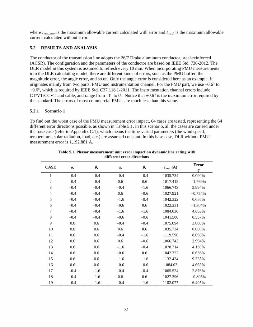
5.2.1 Scenario 1
To find out the worst case of the PMU measurement error impact, 64 cases are tested, representing the 64
different error directions possible, as shown in Table 5.1. In this scenario, all the cases are carried under
the base case (refer to Appendix C.1), which means the time-varied parameters (the wind speed,
temperature, solar radiation, load, etc.) are assumed constant. In this base case, DLR without PMU
measurement error is 1,192.881 A.
Table 5.1. Phasor measurement unit error impact on dynamic line rating with
different error directions
CASE αs βs αr βr Imax (A) Error
η
1 –0.4 –0.4 –0.4 –0.4 1035.734 0.000%
2 –0.4 –0.4 0.6 0.6 1017.415 –1.769%
3 –0.4 –0.4 –0.4 –1.6 1066.743 2.994%
4 –0.4 –0.4 0.6 –0.6 1027.921 –0.754%
5 –0.4 –0.4 –1.6 –0.4 1042.322 0.636%
6 –0.4 –0.4 –0.6 0.6 1022.231 –1.304%
7 –0.4 –0.4 –1.6 –1.6 1084.030 4.663%
8 –0.4 –0.4 –0.6 –0.6 1041.500 0.557%
9 0.6 0.6 –0.4 –0.4 1075.094 3.800%
10 0.6 0.6 0.6 0.6 1035.734 0.000%
11 0.6 0.6 –0.4 –1.6 1119.590 8.096%
12 0.6 0.6 0.6 –0.6 1066.743 2.994%
13 0.6 0.6 –1.6 –0.4 1078.714 4.150%
14 0.6 0.6 –0.6 0.6 1042.322 0.636%
15 0.6 0.6 –1.6 –1.6 1132.424 9.335%
16 0.6 0.6 –0.6 –0.6 1084.03 4.663%
17 –0.4 –1.6 –0.4 –0.4 1065.524 2.876%
18 –0.4 –1.6 0.6 0.6 1027.396 –0.805%
19 –0.4 –1.6 –0.4 –1.6 1102.077 6.405%
32
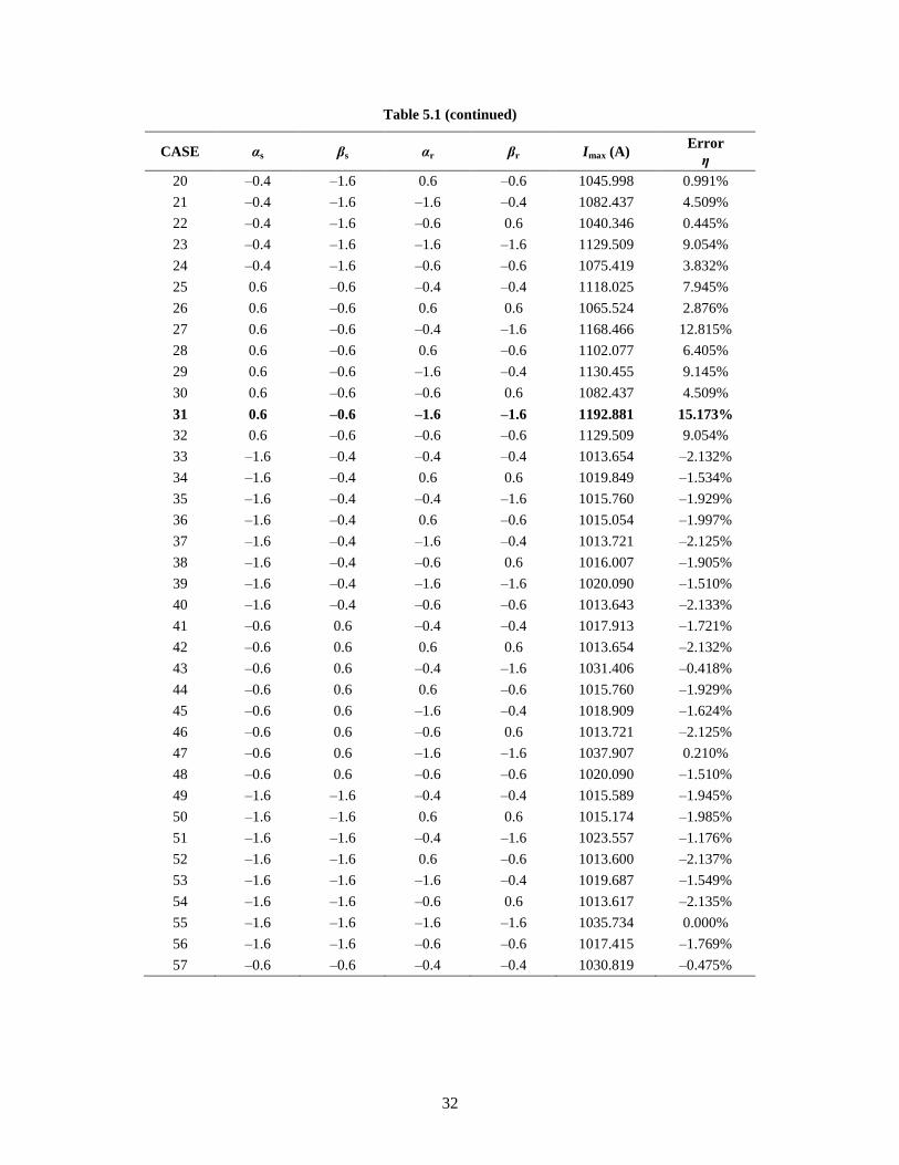
Table 5.1 (continued)
CASE αs βs αr βr Imax (A) Error
η
20 –0.4 –1.6 0.6 –0.6 1045.998 0.991%
21 –0.4 –1.6 –1.6 –0.4 1082.437 4.509%
22 –0.4 –1.6 –0.6 0.6 1040.346 0.445%
23 –0.4 –1.6 –1.6 –1.6 1129.509 9.054%
24 –0.4 –1.6 –0.6 –0.6 1075.419 3.832%
25 0.6 –0.6 –0.4 –0.4 1118.025 7.945%
26 0.6 –0.6 0.6 0.6 1065.524 2.876%
27 0.6 –0.6 –0.4 –1.6 1168.466 12.815%
28 0.6 –0.6 0.6 –0.6 1102.077 6.405%
29 0.6 –0.6 –1.6 –0.4 1130.455 9.145%
30 0.6 –0.6 –0.6 0.6 1082.437 4.509%
31 0.6 –0.6 –1.6 –1.6 1192.881 15.173%
32 0.6 –0.6 –0.6 –0.6 1129.509 9.054%
33 –1.6 –0.4 –0.4 –0.4 1013.654 –2.132%
34 –1.6 –0.4 0.6 0.6 1019.849 –1.534%
35 –1.6 –0.4 –0.4 –1.6 1015.760 –1.929%
36 –1.6 –0.4 0.6 –0.6 1015.054 –1.997%
37 –1.6 –0.4 –1.6 –0.4 1013.721 –2.125%
38 –1.6 –0.4 –0.6 0.6 1016.007 –1.905%
39 –1.6 –0.4 –1.6 –1.6 1020.090 –1.510%
40 –1.6 –0.4 –0.6 –0.6 1013.643 –2.133%
41 –0.6 0.6 –0.4 –0.4 1017.913 –1.721%
42 –0.6 0.6 0.6 0.6 1013.654 –2.132%
43 –0.6 0.6 –0.4 –1.6 1031.406 –0.418%
44 –0.6 0.6 0.6 –0.6 1015.760 –1.929%
45 –0.6 0.6 –1.6 –0.4 1018.909 –1.624%
46 –0.6 0.6 –0.6 0.6 1013.721 –2.125%
47 –0.6 0.6 –1.6 –1.6 1037.907 0.210%
48 –0.6 0.6 –0.6 –0.6 1020.090 –1.510%
49 –1.6 –1.6 –0.4 –0.4 1015.589 –1.945%
50 –1.6 –1.6 0.6 0.6 1015.174 –1.985%
51 –1.6 –1.6 –0.4 –1.6 1023.557 –1.176%
52 –1.6 –1.6 0.6 –0.6 1013.600 –2.137%
53 –1.6 –1.6 –1.6 –0.4 1019.687 –1.549%
54 –1.6 –1.6 –0.6 0.6 1013.617 –2.135%
55 –1.6 –1.6 –1.6 –1.6 1035.734 0.000%
56 –1.6 –1.6 –0.6 –0.6 1017.415 –1.769%
57 –0.6 –0.6 –0.4 –0.4 1030.819 –0.475%
33
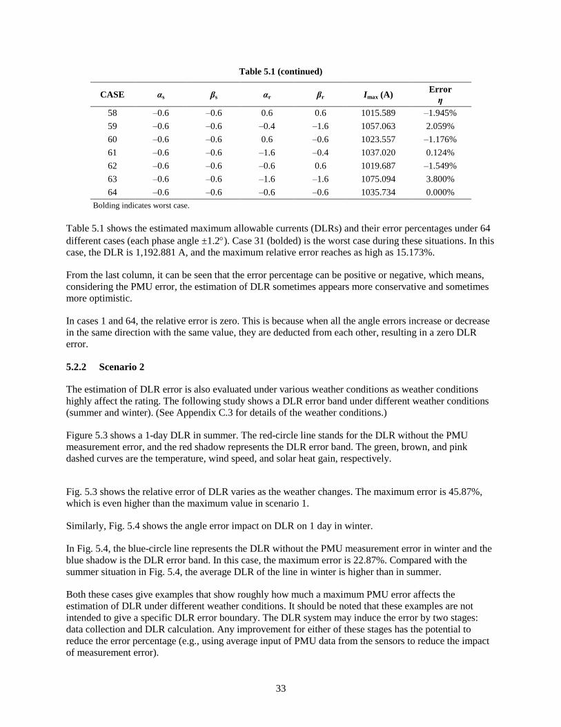
Table 5.1 (continued)
CASE αs βs αr βr Imax (A) Error
η
58 –0.6 –0.6 0.6 0.6 1015.589 –1.945%
59 –0.6 –0.6 –0.4 –1.6 1057.063 2.059%
60 –0.6 –0.6 0.6 –0.6 1023.557 –1.176%
61 –0.6 –0.6 –1.6 –0.4 1037.020 0.124%
62 –0.6 –0.6 –0.6 0.6 1019.687 –1.549%
63 –0.6 –0.6 –1.6 –1.6 1075.094 3.800%
64 –0.6 –0.6 –0.6 –0.6 1035.734 0.000%
Bolding indicates worst case.
Table 5.1 shows the estimated maximum allowable currents (DLRs) and their error percentages under 64
different cases (each phase angle ±1.2). Case 31 (bolded) is the worst case during these situations. In this
case, the DLR is 1,192.881 A, and the maximum relative error reaches as high as 15.173%.
From the last column, it can be seen that the error percentage can be positive or negative, which means,
considering the PMU error, the estimation of DLR sometimes appears more conservative and sometimes
more optimistic.
In cases 1 and 64, the relative error is zero. This is because when all the angle errors increase or decrease
in the same direction with the same value, they are deducted from each other, resulting in a zero DLR
error.
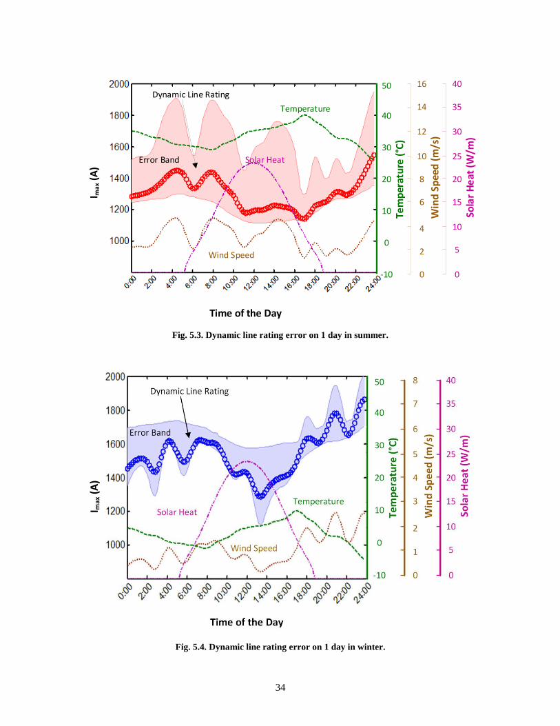
5.2.2 Scenario 2
The estimation of DLR error is also evaluated under various weather conditions as weather conditions
highly affect the rating. The following study shows a DLR error band under different weather conditions
(summer and winter). (See Appendix C.3 for details of the weather conditions.)
Figure 5.3 shows a 1-day DLR in summer. The red-circle line stands for the DLR without the PMU
measurement error, and the red shadow represents the DLR error band. The green, brown, and pink
dashed curves are the temperature, wind speed, and solar heat gain, respectively.
Fig. 5.3 shows the relative error of DLR varies as the weather changes. The maximum error is 45.87%,
which is even higher than the maximum value in scenario 1.
Similarly, Fig. 5.4 shows the angle error impact on DLR on 1 day in winter.
In Fig. 5.4, the blue-circle line represents the DLR without the PMU measurement error in winter and the
blue shadow is the DLR error band. In this case, the maximum error is 22.87%. Compared with the
summer situation in Fig. 5.4, the average DLR of the line in winter is higher than in summer.
Both these cases give examples that show roughly how much a maximum PMU error affects the
estimation of DLR under different weather conditions. It should be noted that these examples are not
intended to give a specific DLR error boundary. The DLR system may induce the error by two stages:
data collection and DLR calculation. Any improvement for either of these stages has the potential to
reduce the error percentage (e.g., using average input of PMU data from the sensors to reduce the impact
of measurement error).
34
Tem
per
atu
re (
°C)
-10
0
20
30
40
50
10 Win
d S
pee
d (
m/s
)
0
2
8
10
14
16
6
4
12
Sola
r H
eat
(W
/m)
0
5
20
25
35
40
15
10
30
Temperature
Solar Heat
Wind Speed
Error Band
Dynamic Line Rating
Time of the Day
I max
(A
)
Fig. 5.3. Dynamic line rating error on 1 day in summer.
I ma
x (A
)
Fig. 5.4. Dynamic line rating error on 1 day in winter.
35
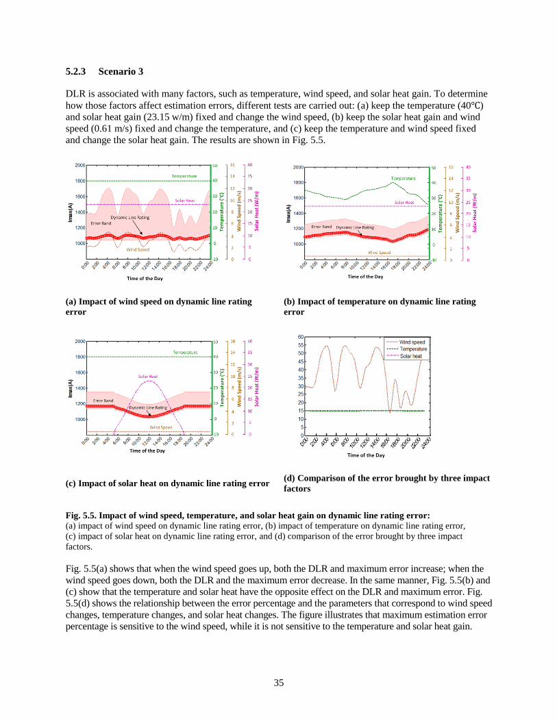
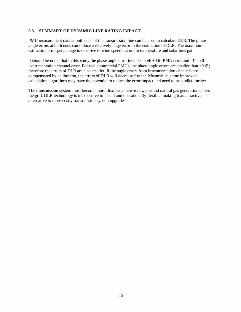
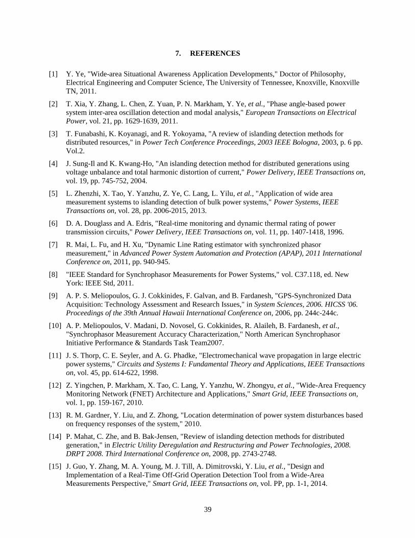
5.2.3 Scenario 3
DLR is associated with many factors, such as temperature, wind speed, and solar heat gain. To determine
how those factors affect estimation errors, different tests are carried out: (a) keep the temperature (40℃)
and solar heat gain (23.15 w/m) fixed and change the wind speed, (b) keep the solar heat gain and wind
speed (0.61 m/s) fixed and change the temperature, and (c) keep the temperature and wind speed fixed
and change the solar heat gain. The results are shown in Fig. 5.5.
(a) Impact of wind speed on dynamic line rating
error
(b) Impact of temperature on dynamic line rating
error
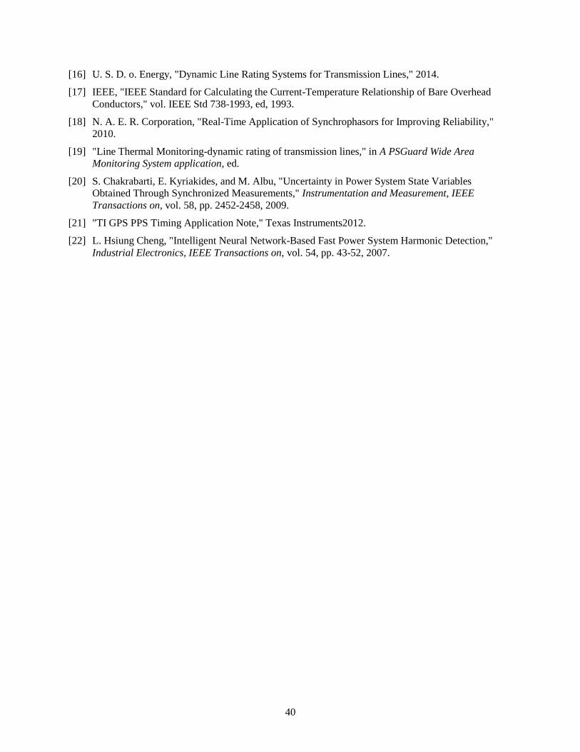
(c) Impact of solar heat on dynamic line rating error (d) Comparison of the error brought by three impact
factors
Fig. 5.5. Impact of wind speed, temperature, and solar heat gain on dynamic line rating error: (a) impact of wind speed on dynamic line rating error, (b) impact of temperature on dynamic line rating error,
(c) impact of solar heat on dynamic line rating error, and (d) comparison of the error brought by three impact
factors.
Fig. 5.5(a) shows that when the wind speed goes up, both the DLR and maximum error increase; when the
wind speed goes down, both the DLR and the maximum error decrease. In the same manner, Fig. 5.5(b) and
(c) show that the temperature and solar heat have the opposite effect on the DLR and maximum error. Fig.
5.5(d) shows the relationship between the error percentage and the parameters that correspond to wind speed
changes, temperature changes, and solar heat changes. The figure illustrates that maximum estimation error
percentage is sensitive to the wind speed, while it is not sensitive to the temperature and solar heat gain.
36
5.3 SUMMARY OF DYNAMIC LINE RATING IMPACT
PMU measurement data at both ends of the transmission line can be used to calculate DLR. The phase
angle errors at both ends can induce a relatively huge error in the estimation of DLR. The maximum
estimation error percentage is sensitive to wind speed but not to temperature and solar heat gain.
It should be noted that in this study the phase angle error includes both ±0.6 PMU error and –1 to 0
instrumentation channel error. For real commercial PMUs, the phase angle errors are smaller than ±0.6;
therefore the errors of DLR are also smaller. If the angle errors from instrumentation channels are
compensated by calibration, the errors of DLR will decrease further. Meanwhile, some improved
calculation algorithms may have the potential to reduce the error impact and need to be studied further.
The transmission system must become more flexible as new renewable and natural gas generation enters
the grid. DLR technology is inexpensive to install and operationally flexible, making it an attractive
alternative to more costly transmission system upgrades.

37
6. CONCLUSION
In this report, the impact of synchrophasor measurement error on several applications is analyzed. The
results are included in Table 6.1
Table 6.1. Effect of measurement error on applications
Application Effect Significance
Event location A small number of cases show impact Minor impact typically
Oscillation detection Possible failure detection or false alarm Threshold dependent
Islanding detection Not likely to be influenced for detection time
above 2 s Detection time dependent
Dynamic line rating Potential to induce huge error. Very sensitive
It can be seen from the table that the DLR application is more likely to be influenced by measurement
error. It is possible for the oscillation to be submerged by the error, resulting in detection failure. It is also
possible for a nonoscillation to be reported as a result of error. Both depend on the threshold. For
islanding detection, when the required detection time is equal to or above 2 s, it is unlikely to be
influenced by the measurement error. For event location, the error in most cases is not likely to impact the
result.
The PMU errors used in this study are taken from IEEE Std. C37.118.1-2011 as the minimum required
for PMUs. We need to point out that many commercial PMUs, as well as the FDRs from UTK/ORNL,
have a much higher level of accuracy. For example, one commercial PMU we tested has an angle
accuracy of 0.005 degree and frequency accuracy of 0.1 mHz. The UTK/ORNL FDR has an angle
accuracy of 0.005 degree and frequency accuracy of 0.06 mHz. In a future study, it may be more realistic
to use typical industry accuracy levels for an assessment.

39
7. REFERENCES
[1] Y. Ye, "Wide-area Situational Awareness Application Developments," Doctor of Philosophy,
Electrical Engineering and Computer Science, The University of Tennessee, Knoxville, Knoxville
TN, 2011.
[2] T. Xia, Y. Zhang, L. Chen, Z. Yuan, P. N. Markham, Y. Ye, et al., "Phase angle-based power
system inter-area oscillation detection and modal analysis," European Transactions on Electrical
Power, vol. 21, pp. 1629-1639, 2011.
[3] T. Funabashi, K. Koyanagi, and R. Yokoyama, "A review of islanding detection methods for
distributed resources," in Power Tech Conference Proceedings, 2003 IEEE Bologna, 2003, p. 6 pp.
Vol.2.
[4] J. Sung-Il and K. Kwang-Ho, "An islanding detection method for distributed generations using
voltage unbalance and total harmonic distortion of current," Power Delivery, IEEE Transactions on,
vol. 19, pp. 745-752, 2004.
[5] L. Zhenzhi, X. Tao, Y. Yanzhu, Z. Ye, C. Lang, L. Yilu, et al., "Application of wide area
measurement systems to islanding detection of bulk power systems," Power Systems, IEEE
Transactions on, vol. 28, pp. 2006-2015, 2013.
[6] D. A. Douglass and A. Edris, "Real-time monitoring and dynamic thermal rating of power
transmission circuits," Power Delivery, IEEE Transactions on, vol. 11, pp. 1407-1418, 1996.
[7] R. Mai, L. Fu, and H. Xu, "Dynamic Line Rating estimator with synchronized phasor
measurement," in Advanced Power System Automation and Protection (APAP), 2011 International
Conference on, 2011, pp. 940-945.
[8] "IEEE Standard for Synchrophasor Measurements for Power Systems," vol. C37.118, ed. New
York: IEEE Std, 2011.
[9] A. P. S. Meliopoulos, G. J. Cokkinides, F. Galvan, and B. Fardanesh, "GPS-Synchronized Data
Acquisition: Technology Assessment and Research Issues," in System Sciences, 2006. HICSS '06.
Proceedings of the 39th Annual Hawaii International Conference on, 2006, pp. 244c-244c.
[10] A. P. Meliopoulos, V. Madani, D. Novosel, G. Cokkinides, R. Alaileh, B. Fardanesh, et al.,
"Synchrophasor Measurement Accuracy Characterization," North American Synchrophasor
Initiative Performance & Standards Task Team2007.
[11] J. S. Thorp, C. E. Seyler, and A. G. Phadke, "Electromechanical wave propagation in large electric
power systems," Circuits and Systems I: Fundamental Theory and Applications, IEEE Transactions
on, vol. 45, pp. 614-622, 1998.
[12] Z. Yingchen, P. Markham, X. Tao, C. Lang, Y. Yanzhu, W. Zhongyu, et al., "Wide-Area Frequency
Monitoring Network (FNET) Architecture and Applications," Smart Grid, IEEE Transactions on,
vol. 1, pp. 159-167, 2010.
[13] R. M. Gardner, Y. Liu, and Z. Zhong, "Location determination of power system disturbances based
on frequency responses of the system," 2010.
[14] P. Mahat, C. Zhe, and B. Bak-Jensen, "Review of islanding detection methods for distributed
generation," in Electric Utility Deregulation and Restructuring and Power Technologies, 2008.
DRPT 2008. Third International Conference on, 2008, pp. 2743-2748.
[15] J. Guo, Y. Zhang, M. A. Young, M. J. Till, A. Dimitrovski, Y. Liu, et al., "Design and
Implementation of a Real-Time Off-Grid Operation Detection Tool from a Wide-Area
Measurements Perspective," Smart Grid, IEEE Transactions on, vol. PP, pp. 1-1, 2014.
40
[16] U. S. D. o. Energy, "Dynamic Line Rating Systems for Transmission Lines," 2014.
[17] IEEE, "IEEE Standard for Calculating the Current-Temperature Relationship of Bare Overhead
Conductors," vol. IEEE Std 738-1993, ed, 1993.
[18] N. A. E. R. Corporation, "Real-Time Application of Synchrophasors for Improving Reliability,"
2010.
[19] "Line Thermal Monitoring-dynamic rating of transmission lines," in A PSGuard Wide Area
Monitoring System application, ed.
[20] S. Chakrabarti, E. Kyriakides, and M. Albu, "Uncertainty in Power System State Variables
Obtained Through Synchronized Measurements," Instrumentation and Measurement, IEEE
Transactions on, vol. 58, pp. 2452-2458, 2009.
[21] "TI GPS PPS Timing Application Note," Texas Instruments2012.
[22] L. Hsiung Cheng, "Intelligent Neural Network-Based Fast Power System Harmonic Detection,"
Industrial Electronics, IEEE Transactions on, vol. 54, pp. 43-52, 2007.

APPENDIX A. APPLICATIONS OF PHASOR MEASUREMENT UNITS

A-3
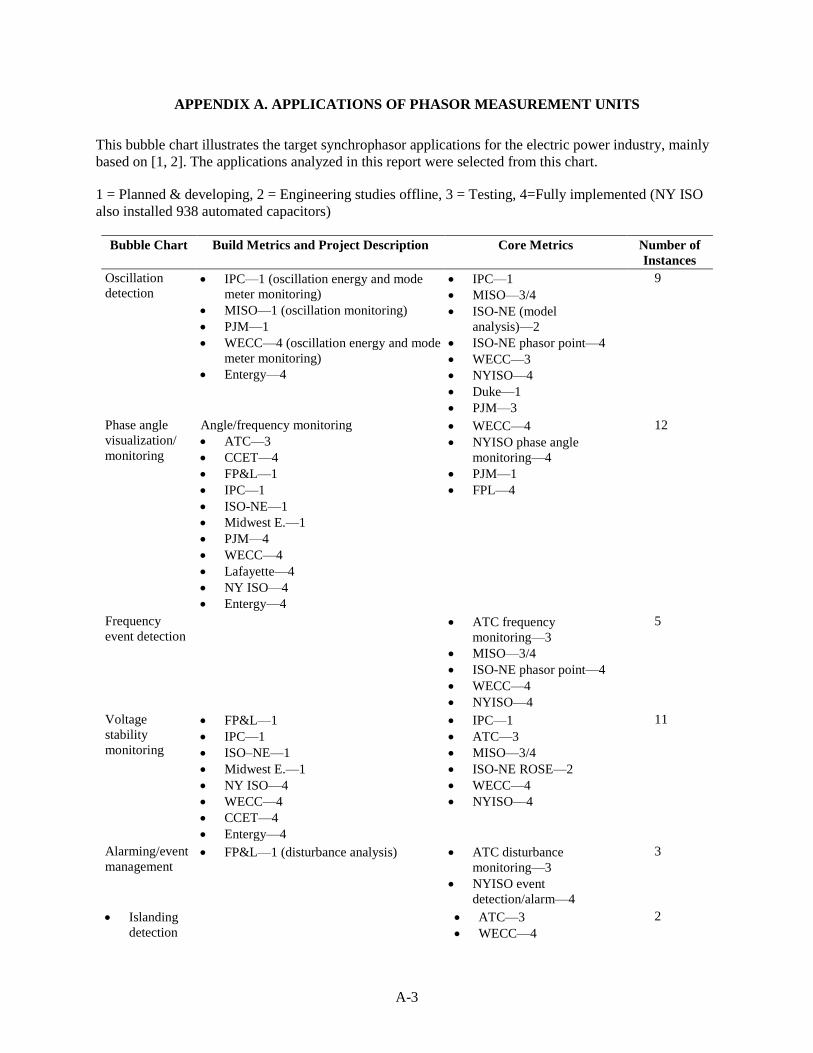
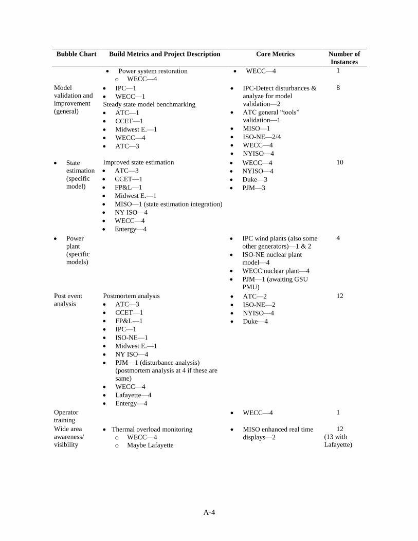
APPENDIX A. APPLICATIONS OF PHASOR MEASUREMENT UNITS
This bubble chart illustrates the target synchrophasor applications for the electric power industry, mainly
based on [1, 2]. The applications analyzed in this report were selected from this chart.
1 = Planned & developing, 2 = Engineering studies offline, 3 = Testing, 4=Fully implemented (NY ISO
also installed 938 automated capacitors)
Bubble Chart Build Metrics and Project Description Core Metrics Number of
Instances
Oscillation
detection IPC—1 (oscillation energy and mode
meter monitoring)
MISO—1 (oscillation monitoring)
PJM—1
WECC—4 (oscillation energy and mode
meter monitoring)
Entergy—4
IPC—1
MISO—3/4
ISO-NE (model
analysis)—2
ISO-NE phasor point—4
WECC—3
NYISO—4
Duke—1
PJM—3
9
Phase angle
visualization/
monitoring
Angle/frequency monitoring
ATC—3
CCET—4
FP&L—1
IPC—1
ISO-NE—1
Midwest E.—1
PJM—4
WECC—4
Lafayette—4
NY ISO—4
Entergy—4
WECC—4
NYISO phase angle
monitoring—4
PJM—1
FPL—4
12
Frequency
event detection
ATC frequency
monitoring—3
MISO—3/4
ISO-NE phasor point—4
WECC—4
NYISO—4
5
Voltage
stability
monitoring
FP&L—1
IPC—1
ISO–NE—1
Midwest E.—1
NY ISO—4
WECC—4
CCET—4
Entergy—4
IPC—1
ATC—3
MISO—3/4
ISO-NE ROSE—2
WECC—4
NYISO—4
11
Alarming/event
management FP&L—1 (disturbance analysis) ATC disturbance
monitoring—3
NYISO event
detection/alarm—4
3
Islanding
detection
ATC—3
WECC—4
2
A-4
Bubble Chart Build Metrics and Project Description Core Metrics Number of
Instances
Power system restoration
o WECC—4
WECC—4 1
Model
validation and
improvement
(general)
IPC—1
WECC—1
Steady state model benchmarking
ATC—1
CCET—1
Midwest E.—1
WECC—4
ATC—3
IPC-Detect disturbances &
analyze for model
validation—2
ATC general “tools”
validation—1
MISO—1
ISO-NE—2/4
WECC—4
NYISO—4
8
State
estimation
(specific
model)
Improved state estimation
ATC—3
CCET—1
FP&L—1
Midwest E.—1
MISO—1 (state estimation integration)
NY ISO—4
WECC—4
Entergy—4
WECC—4
NYISO—4
Duke—3
PJM—3
10
Power
plant
(specific
models)
IPC wind plants (also some
other generators)—1 & 2
ISO-NE nuclear plant
model—4
WECC nuclear plant—4
PJM—1 (awaiting GSU
PMU)
4
Post event
analysis
Postmortem analysis
ATC—3
CCET—1
FP&L—1
IPC—1
ISO-NE—1
Midwest E.—1
NY ISO—4
PJM—1 (disturbance analysis)
(postmortem analysis at 4 if these are
same)
WECC—4
Lafayette—4
Entergy—4
ATC—2
ISO-NE—2
NYISO—4
Duke—4
12
Operator
training
WECC—4 1
Wide area
awareness/
visibility
Thermal overload monitoring
o WECC—4
o Maybe Lafayette
MISO enhanced real time
displays—2
12
(13 with
Lafayette)

A-5
Bubble Chart Build Metrics and Project Description Core Metrics Number of
Instances
General Monitoring/Visualization
o FP&L—1
o IPC—1 (reactive reserves
monitoring)
o IPC—1 (path loading and
congestion management)
o MISO—1
o PJM—1
o CCET—4 (RTDMS, build baseline)
o WECC—1 (reactive reserves
monitoring & device control)
o WECC—1 (path loading &
congestion management)
o ATC—2
o Entergy—4
ISO-NE—2
ISO-NE ROSE—2
WECC—4
NYISO—3
Duke—4
PJM—4
DG/IPP applications none
General event
detection FP&L—1
ISO-NE—1 (disturbance detection)
MISO—1
Entergy—4
ATC—1
MISO—3/4
ISO-NE phasor point—4;
ROSE—2
WECC—4
PJM—1
FPL (equipment health)—4
8
Identify a
specific
problem
(generator,
substation…)
(case study or
event instance,
not application)
MISO
FPL
WECC
ISO-NE
Not an
application—
just added for
general
information
PMU data
quality
monitoring/
improvement
ISO-NE—4
PJM—4
Description:
Separate bullets for all instances of a recipient having this application
o Solid bullet if the application is a category
o Circle bullet if the application is a subcategory
First column is based on [1, 2].
o Rows that begin with “bullets” are subsets of special cases of the overall category
Second column is the list of applications from the Build Metrics and project descriptions on the
website (https://smartgrid.gov/sites/default/files/synchrophasor_project_status_110114-3.pdf), and instances
(recipients) if reported there
o If the application is the same or similar to one in the first column, it is in the same line as the first
column
o If the application is a subset of the first column, it is listed as a bullet
Third column is instances (recipients) of column 1 application mentioned in core metrics
Fourth column (number of instances) = number if in {column 2 OR column 3}

A-6
REFERENCES
[1] (2014, Dec). Recovery Act Smart Grid Investments Synchrophasor Project Status. Available:
https://www.smartgrid.gov/sites/default/files/synchrophasor_project_status_110114-3.pdf.
[2] SMARTGRID.GOV, "Factors Affecting PMU Installation Costs," 2014.

APPENDIX B. DYNAMIC LINE RATING MODEL

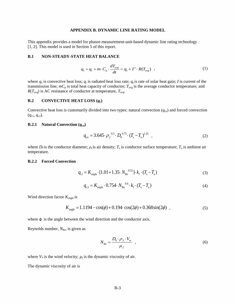
B-3
APPENDIX B. DYNAMIC LINE RATING MODEL
This appendix provides a model for phasor-measurement-unit-based dynamic line rating technology
[1, 2]. This model is used in Section 5 of this report.
B.1 NON-STEADY-STATE HEAT BALANCE
avg 2
c r p s avg( )dT
q q m C q I R Tdt
, (1)
where qc is convective heat loss; qr is radiated heat loss rate; qs is rate of solar heat gain; I is current of the
transmission line; mCp is total heat capacity of conductor; Tavg is the average conductor temperature; and
R(Tavg) is AC resistance of conductor at temperature, Tavg.
B.2 CONVECTIVE HEAT LOSS (qc)
Convective heat loss is customarily divided into two types: natural convection (qcn) and forced convection
(qc1, qc2).
B.2.1 Natural Convection (qcn)
0.5 0.75 1.25
cn 0 s a3.645 ( )fq D T T , (2)
where D0 is the conductor diameter; ρf is air density; Ts is conductor surface temperature; Ta is ambient air
temperature.
B.2.2 Forced Convection
0.52
1 Re f s a[1.01 1.35 ] ( )c angleq K N k T T (3)
0.6
2 Re f s a0.754 ( )c angleq K N k T T (4)
Wind direction factor Kangle is
angle 1.1194 cos( ) 0.194 cos(2 ) 0.368sin(2 )K , (5)
where φ is the angle between the wind direction and the conductor axis.
Reynolds number, NRe, is given as
0 w
Re
f
f
D VN
, (6)
where Vw is the wind velocity; µf is the dynamic viscosity of air.
The dynamic viscosity of air is
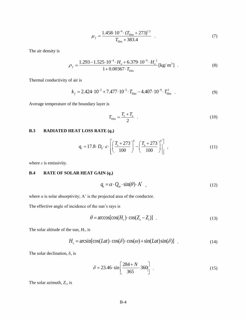
B-4
6 1.5
film
film
1.458 10 ( 273)
383.4f
T
T
. (7)
The air density is
4 9 23
film
1.293 1.525 10 6.379 10[kg/ m ]
1 0.00367
e ef
H H
T
. (8)
Thermal conductivity of air is
2 5 9 2
film film2.424 10 7.477 10 4.407 10fk T T . (9)
Average temperature of the boundary layer is
s afilm
2
T TT
. (10)
B.3 RADIATED HEAT LOSS RATE (qr)
4 4
s ar 0
273 27317.8
100 100
T Tq D
, (11)
where ε is emissivity.
B.4 RATE OF SOLAR HEAT GAIN (qs)
s sin( ) Aseq Q , (12)
where α is solar absorptivity; A’ is the projected area of the conductor.
The effective angle of incidence of the sun’s rays is
c c larccos[cos( ) cos( )]H Z Z . (13)
The solar altitude of the sun, Hc, is
arcsin[cos( ) cos( ) cos( ) sin( )sin( )]cH Lat Lat . (14)
The solar declination, , is
284
23.46 sin 360365
N
. (15)
The solar azimuth, Zc, is
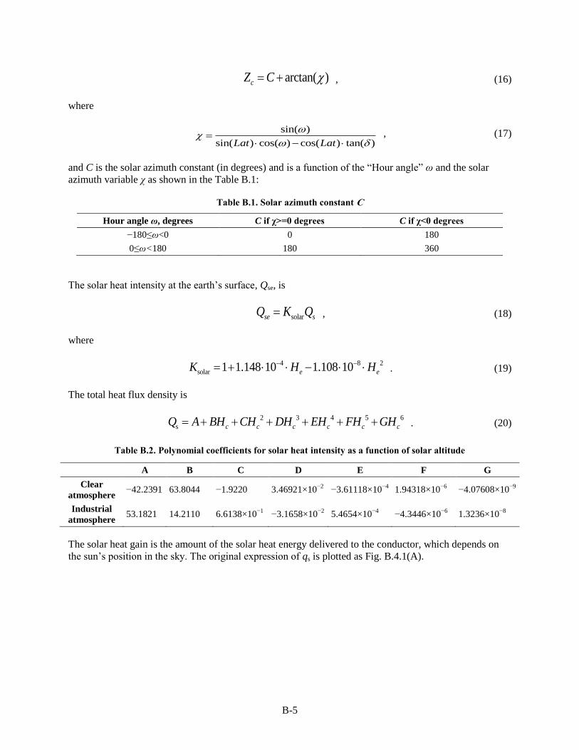
B-5
arctan( )cZ C , (16)
where
sin( )
sin( ) cos( ) cos( ) tan( )Lat Lat
, (17)
and C is the solar azimuth constant (in degrees) and is a function of the “Hour angle” ω and the solar
azimuth variable χ as shown in the Table B.1:
Table B.1. Solar azimuth constant C
Hour angle ω, degrees C if χ>=0 degrees C if χ<0 degrees
−180≤ω<0 0 180
0≤ω<180 180 360
The solar heat intensity at the earth’s surface, Qse, is
solarse sQ K Q , (18)
where
4 8 2
solar 1 1.148 10 1.108 10e eK H H . (19)
The total heat flux density is
2 3 4 5 6
s c c c c c cQ A BH CH DH EH FH GH . (20)
Table B.2. Polynomial coefficients for solar heat intensity as a function of solar altitude
A B C D E F G
Clear
atmosphere −42.2391 63.8044 −1.9220 3.46921×10
−2 −3.61118×10
−4 1.94318×10
−6 −4.07608×10
−9
Industrial
atmosphere 53.1821 14.2110 6.6138×10
−1 −3.1658×10
−2 5.4654×10
−4 −4.3446×10
−6 1.3236×10
−8
The solar heat gain is the amount of the solar heat energy delivered to the conductor, which depends on
the sun’s position in the sky. The original expression of qs is plotted as Fig. B.4.1(A).
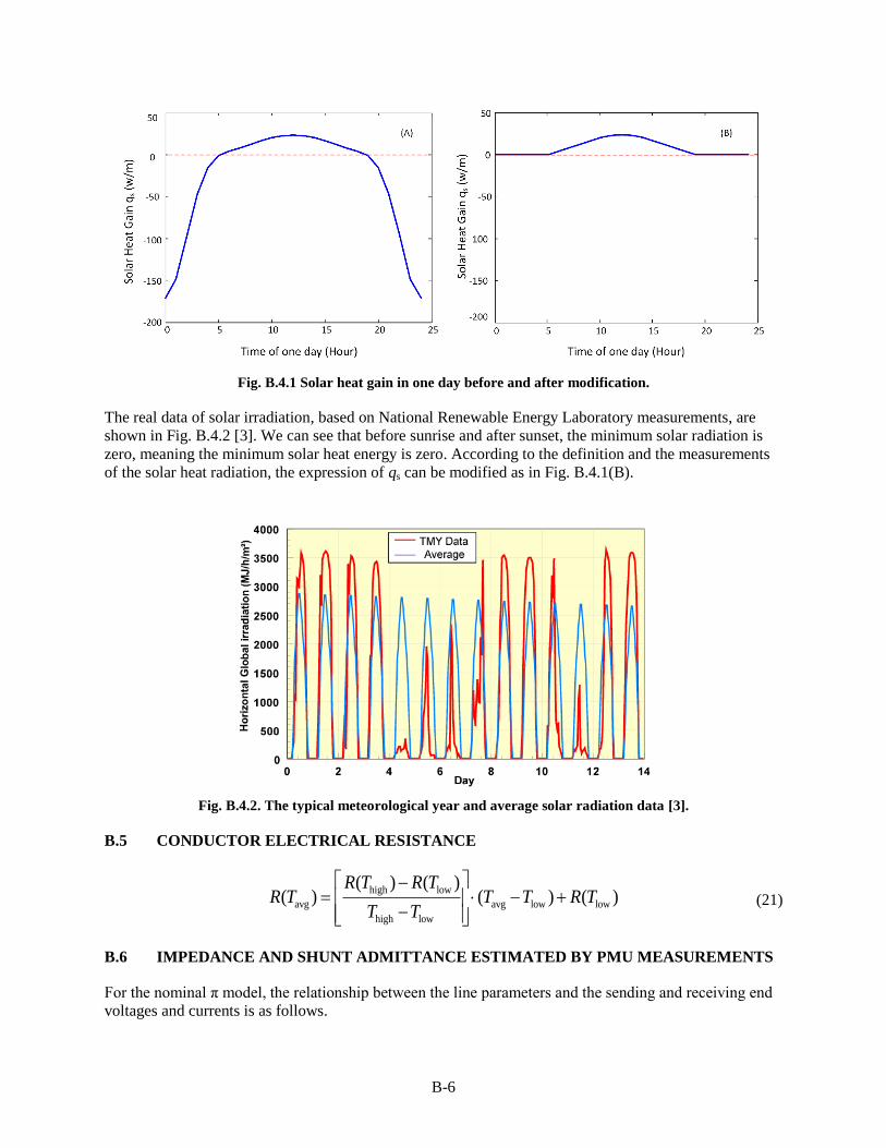
B-6
Fig. B.4.1 Solar heat gain in one day before and after modification.
The real data of solar irradiation, based on National Renewable Energy Laboratory measurements, are
shown in Fig. B.4.2 [3]. We can see that before sunrise and after sunset, the minimum solar radiation is
zero, meaning the minimum solar heat energy is zero. According to the definition and the measurements
of the solar heat radiation, the expression of qs can be modified as in Fig. B.4.1(B).
Fig. B.4.2. The typical meteorological year and average solar radiation data [3].
B.5 CONDUCTOR ELECTRICAL RESISTANCE
high low
avg avg low low
high low
( ) ( )( ) ( ) ( )
R T R TR T T T R T
T T
(21)
B.6 IMPEDANCE AND SHUNT ADMITTANCE ESTIMATED BY PMU MEASUREMENTS
For the nominal π model, the relationship between the line parameters and the sending and receiving end
voltages and currents is as follows.
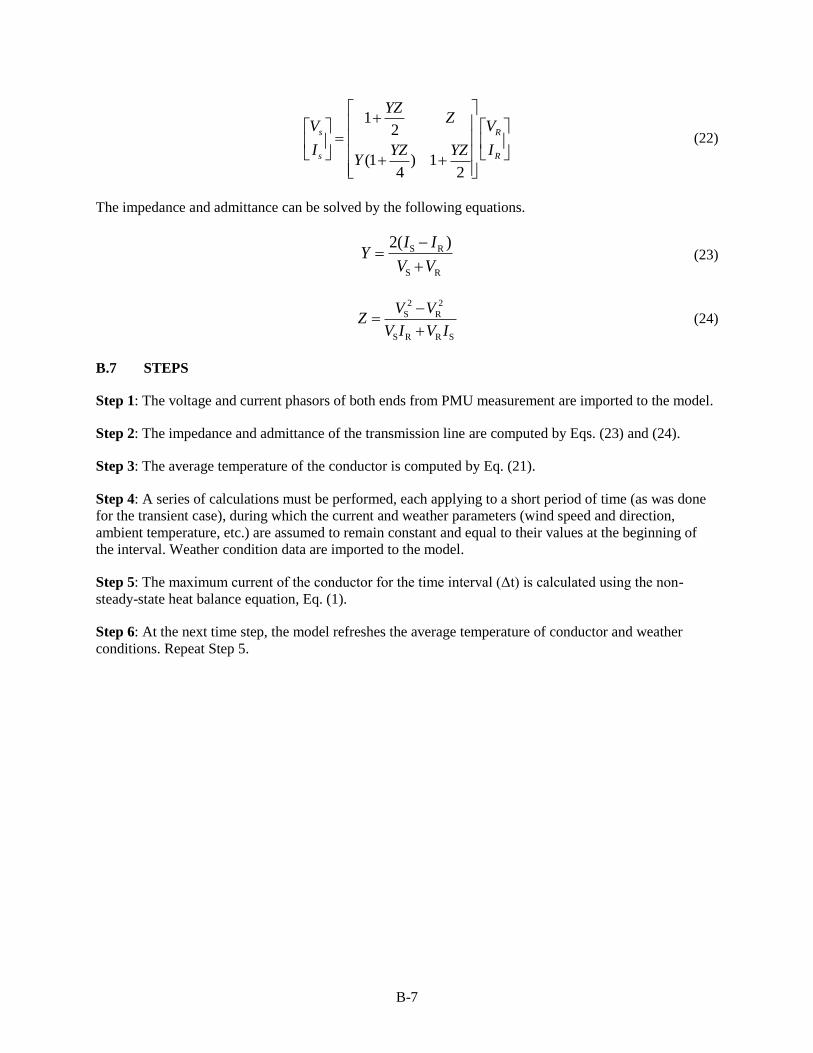
B-7
12
(1 ) 14 2
s R
s R
YZZ
V V
I IYZ YZY
(22)
The impedance and admittance can be solved by the following equations.
S R
S R
2( )I IY
V V
(23)
2 2
S R
S R R S
V VZ
V I V I
(24)
B.7 STEPS
Step 1: The voltage and current phasors of both ends from PMU measurement are imported to the model.
Step 2: The impedance and admittance of the transmission line are computed by Eqs. (23) and (24).
Step 3: The average temperature of the conductor is computed by Eq. (21).
Step 4: A series of calculations must be performed, each applying to a short period of time (as was done
for the transient case), during which the current and weather parameters (wind speed and direction,
ambient temperature, etc.) are assumed to remain constant and equal to their values at the beginning of
the interval. Weather condition data are imported to the model.
Step 5: The maximum current of the conductor for the time interval (Δt) is calculated using the non-
steady-state heat balance equation, Eq. (1).
Step 6: At the next time step, the model refreshes the average temperature of conductor and weather
conditions. Repeat Step 5.
B-8
REFERENCES
[1] IEEE, “IEEE Standard for Calculating the Current-Temperature Relationship of Bare Overhead
Conductors”, IEEE Std 738-1993.
[2] Sveinn Rúnar Júlíusson, “Using PMU Measurements to Assess Dynamic Line Rating of
Transmission Lines”, Aalborg University, 2013.
[3] Analysis of Solar Irradiance Data Sets. Available: http://pveducation.org/pvcdrom/properties-of-
sunlight/analysis-of-solar-irradiance-data-sets.
APPENDIX C. INPUT DATA FOR DYNAMIC LINE RATING MODEL

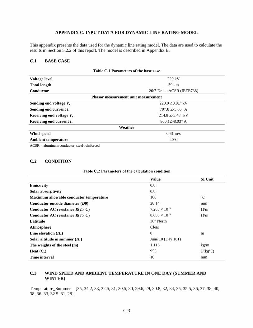
C-3
APPENDIX C. INPUT DATA FOR DYNAMIC LINE RATING MODEL
This appendix presents the data used for the dynamic line rating model. The data are used to calculate the
results in Section 5.2.2 of this report. The model is described in Appendix B.
C.1 BASE CASE
Table C.1 Parameters of the base case
Voltage level 220 kV
Total length 59 km
Conductor 26/7 Drake ACSR (IEEE738)
Phasor measurement unit measurement
Sending end voltage Vs 220.0 ∠0.01° kV
Sending end current Is 797.8 ∠-5.66° A
Receiving end voltage Vr 214.8 ∠-5.48° kV
Receiving end current Ir 800.1∠-8.03° A
Weather
Wind speed 0.61 m/s
Ambient temperature 40℃
ACSR = aluminum conductor, steel-reinforced
C.2 CONDITION
Table C.2 Parameters of the calculation condition
Value SI Unit
Emissivity 0.8
Solar absorptivity 0.8
Maximum allowable conductor temperature 100 ℃
Conductor outside diameter (D0) 28.14 mm
Conductor AC resistance R(25°C) 7.283 × 10⁻⁵
Ω/m
Conductor AC resistance R(75°C) 8.688 × 10⁻⁵
Ω/m
Latitude 30° North
Atmosphere Clear
Line elevation (He) 0 m
Solar altitude in summer (Hc) June 10 (Day 161)
The weights of the steel (m) 1.116 kg/m
Heat (Cp) 955 J/(kg℃)
Time interval 10 min
C.3 WIND SPEED AND AMBIENT TEMPERATURE IN ONE DAY (SUMMER AND
WINTER)
Temperature_Summer = [35, 34.2, 33, 32.5, 31, 30.5, 30, 29.6, 29, 30.8, 32, 34, 35, 35.5, 36, 37, 38, 40,
38, 36, 33, 32.5, 31, 28]

C-4
Windspeed_Summer = [2.1, 2.16, 2.3, 3.6, 4.5, 4, 2, 3.5, 4.6, 4.1, 3.5, 2.1, 3, 3.4, 4.4, 4.2, 3, 1.2, 2.5, 1.4,
2, 1.5, 2, 3.3]
Temperature_Winter = [5, 4.2, 3, 2.5, 1, 0.5, 0, -0.4, -1, 0.8, 2, 4, 5, 5.5, 6, 7, 8, 10, 8, 6, 3, 2.5, 1, -2]
Windspeed_Winter = [0.5, 0.75, 0.63, 0.4, 1.2, 0.8, 0.67, 1.32, 1.35, 1.5, 1.0, 0.79, 0.92, 0.34, 0.4, 0.62,
0.70, 1.2, 2, 1.5, 1.8, 2.6, 1.5, 2]