Improved Radiation and Combustion Routines for aLarge Eddy Simulation Fire Model

KEVIN McGRATTAN, JASON FLOYD, GLENN FORNEY and HOWARD BAUMBuilding and Fire Research LaboratoryNational Institute of Standards and Technology (NIST)Gaithersburg, Maryland, 20899, USA

SIMO HOSTIKKAVTT Building and TransportEspoo, Finland

ABSTRACT

Improvements have been made to the combustion and radiation routines of a large eddysimulation fire model maintained by the National Institute of Standards and Technology.The combustion is based on a single transport equation for the mixture fraction with staterelations that reflect the basic stoichiometry of the reaction. The radiation transport equa-tion is solved using the Finite Volume Method, usually with the gray gas assumption forlarge scale simulations for which soot is the dominant emitter and absorber. To make themodel work for practical fire protection engineering problems, some approximations weremade within the new algorithms. These approximations will be discussed and sample cal-culations presented.

KEY WORDS: finite volume method, large eddy simulation, mixture fraction model

INTRODUCTION

In cooperation with the fire protection engineering community, a large eddy simulation firemodel, Fire Dynamics Simulator (FDS), is being developed at NIST to study fire behaviorand to evaluate the performance of fire protection systems in buildings. Version 1 of FDSwas publicly released in February 2000 [1, 2]. To date, about half of the applications ofthe model have been for design of smoke handling systems and sprinkler/detector activationstudies. The other half consist of residential and industrial fire reconstructions. Throughoutits early development, FDS had been aimed primarily at the first set of applications, butfollowing the initial release it became clear that some improvements to the fundamentalalgorithms were needed to address the second set of applications. The two most obviousneeds were for better combustion and radiation models to handle large fires in relativelysmall spaces, like scenarios involving flashover.

An improved version of FDS, called FDS 2, was released in the fall of 2001. The low Machnumber Navier-Stokes equations of FDS version 1 and their numerical solution based onlarge eddy simulation generally remain the same in FDS 2. What is different are the com-

FIRE SAFETY SCIENCE--PROCEEDINGS OF THE SEVENTH INTERNATIONAL SYMPOSIUM, pp. 827-838 827 Copyright © International Association for Fire Safety Science

bustion and radiation routines. FDS 1 contains a relatively simple combustion model thatutilizes “thermal elements,” massless particles that are convected with the flow and re-lease heat at a specified rate. While this model is easy to implement and relatively cheapcomputationally, it lacks the necessary physics to accommodate underventilated fires. Amethod that handles oxygen consumption more naturally includes an equation for a con-served scalar quantity, known as the mixture fraction, that tracks the fuel and product gasesthrough the entire combustion process. The model assumes that the reaction of fuel andoxygen is infinitely fast, an appropriate assumption given the limited resolvable length andtime scales of most practical simulations.

Radiation transport in FDS version 1 was based on a simple algorithm whereby a pre-scribed fraction of the fire’s energy was distributed on surrounding walls according to apoint source approximation. The fire itself was idealized as a discrete set of Lagrangianparticles, referred to as “thermal elements,” that released convective and radiative energyonto the numerical grid. This method had two major problems. The first was that only thefire itself radiated; there was no wall to wall or gas to gas radiative heat transfer. Second,the method became expensive when the fire began to occupy a large fraction of the space.A better method for handling radiative heat transfer is to return to the fundamental radiationtransport equation for a non-scattering gray gas. The equation is solved using techniquessimilar to those for convective transport in finite volume methods for fluid flow, thus thename given to it is the Finite Volume Method (FVM).

The new combustion and radiation routines allow for calculations in which the fire itselfand the thermal insult to nearby objects can be studied in more detail than before whenthe fire was merely a point source of heat and smoke. Studies have been performed toexamine in detail small scale experiments like the cone calorimeter [3], and fundamentalfire scenarios like pool fires [4, 5] and small compartment fires [6]. These calculationsare finely resolved, with grid cells ranging from a few millimeters to a few centimeters.However, the majority of model users are still interested mainly in smoke and heat transportin increasingly complex spaces. The challenge to the model developers is to serve both theresearchers and practitioners with a tool that contains the appropriate level of fire physicsfor the problem at hand. This paper describes how the model was improved to betterdescribe the combustion and radiation phenomena, while at the same time maintain itsrobust hydrodynamic transport routines to handle large scale smoke movement problems.

COMBUSTION

The simplest combustion model that includes the basic stoichiometry of the reaction as-sumes that the fuel, the oxygen, and the combustion products can be related to a singleconserved quantity called the mixture fraction. The obvious advantage of the mixture frac-tion approach is that all of the species transport equations are combined into one, reducingthe computational cost. The mixture fraction combustion model is based on the assumptionthat large scale convective and radiative transport phenomena can be simulated directly, butphysical processes occurring at small length and time scales must be represented in an ap-proximate manner. In short, the model adopted here is based on the assumption that thecombustion occurs much more rapidly than the resolvable convective and diffusive phe-

828

nomena. These same assumptions were made in FDS version 1, where Lagrangian parti-clesknown as “thermal elements” were used to represent small packets of unburned fuel.The problem with this idea was that the elements were pre-programmed to release theirenergy in a given amount of time; the time being derived from flame height correlations ofwell-ventilated fires. The method broke down when the fire became under-ventilated, oreven if the fire was pushed up against a wall [4].

The mixture fraction,Z, is a conserved quantity representing the fraction of gas at a givenpoint that was originally fuel. The mass fractions of all of the major reactants and productscan be derived from the mixture fraction by means of “state relations,” empirical expres-sions arrived at by a combination of simplified analysis and measurement. Start with ageneral reaction between a fuel and oxygen:

νO[O]+νF [F ]→∑P

νP[P] (1)

The numbersνO, νF andνP are the stoichiometric coefficients for the overall combustionprocess that reacts fuel “F” with oxygen “O” to produce a number of products “P”. The sto-ichiometric equation (1) implies that the mass consumption rates for fuel, ˙m′′′

F , and oxidizer,m′′′

O , are related as follows:m′′′

F

νFMF=

m′′′O

νOMO(2)

Underthese assumptions, the mixture fractionZ is defined as:

Z =sYF −

(YO−Y∞

O

)sYI

F +Y∞O

; s=νOMO

νFMF(3)

By design, it varies fromZ = 1 in a region containing only fuel toZ = 0 where the oxygenmass fraction takes on its undepleted ambient value,Y∞

O . Note thatYIF is the fraction of fuel

in the fuel stream. The quantitiesMF , MO, νF andνO are the fuel and oxygen molecularweights and stoichiometric coefficients, respectively. The mixture fractionZ satisfies theconservation law

∂ρZ∂t

+∇ ·ρuZ = ∇ ·ρD∇Z (4)

whereρ is the gas density,D is the material diffusivity, andu is the flow velocity. Equa-tion (4) is a linear combination of the fuel and oxygen mass conservation equations. Theassumption that the chemistry is “fast” means that the reaction that consumes fuel and oxy-gen occurs so rapidly that the fuel and oxygen cannot co-exist. The interface between fueland oxygen is the “flame sheet” defined by

Z(x, t) = Zf ; Zf =Y∞

O

sYIF +Y∞

O

(5)

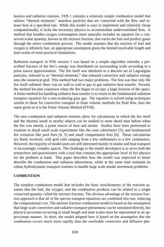
Becausethe mixture fraction is a linear combination of fuel and oxygen, additional in-formation is needed to extract the mass fractions of the major species from the mixturefraction. This information comes in the form of “state relations.” Relations for the majorcomponents of a simple one-step hydrocarbon reaction are given in Fig. 1.

829

FIGURE 1: State relations for propane.

An expression for the local heat release rate can be derived from the conservation equationfor the mixture fraction and the state relation for oxygen. The starting point is Huggett’srelationship for the heat release rate as a function of the oxygen consumption rate

q′′′ = ∆HOm′′′O (6)

Here,∆HO is the heat release rate per unit mass of oxygen consumed, an input parameterto the model that is usually on the order of 13,000 kJ/kg [7]. Equation (6) is the basis foroxygen-consumption calorimetry, and it is consistent with the assumption of infinite-ratekinetics. The oxygen mass conservation equation

ρDYO

Dt= ∇ ·ρD∇YO + m′′′

O (7)

canbe transformed into an expression for the local heat release rate using the conservationequation for the mixture fraction (4) and the state relation for oxygenYO(Z).

−m′′′O = ∇ ·

(ρD

dYO

dZ∇Z

)− dYO

dZ∇ ·ρD∇Z = ρD

d2YO

dZ2 |∇Z|2 (8)

Neitherof these expressions for the local oxygen consumption rate is particularly conve-nient to apply numerically because of the discontinuity of the derivative ofYO(Z) atZ = Zf

for the ideal state relations. However, an expression for the oxygen consumption rate perunit area of flame sheet can be derived from Eq. (8)

−m′′O =

dYO

dZ

∣∣∣∣Z<Zf

ρD ∇Z ·n (9)

In the numerical algorithm, the local heat release rate is computed by first locating theflame sheet, then computing the local heat release rate per unit area, and finally distributing

830

this energy to the grid cells cut by the flame sheet. In this way, the ideal, infinitessimallythin flame sheet is smeared out over the width of a grid cell, consistent with all other gasphase quantities.

RADIATION

Version 1 of FDS had a simple radiation transport algorithm that used randomly chosenrays from energy-carrying Lagrangian particles to walls and other solid obstructions. Thismethod has two major problems. The first is that only the fire itself radiates; there is nowall to wall or gas to gas radiative heat transfer. Second, the method becomes expensivewhen the fire begins to occupy a large fraction of the space. A better method for handlingradiative heat transfer is to consider the Radiative Transport Equation (RTE) for a non-scattering gas

s·∇Iλ(x,s) =κ(x,λ) [Ib(x)− I(x,s)] (10)

where Iλ(x,s) is the radiation intensity at wavelengthλ, Ib(x) is the source term givenby the Planck function,s is the unit normal direction vector andκ(x,λ) is the absorptioncoefficient at a pointx for wavelengthλ.

For practical simulations, the spectral dependence cannot be resolved accurately. Instead,the radiation spectrum can be divided into a relatively small number of bands, and a sep-arate RTE derived for each one [3]. However, even with a small number of bands, thesolution of the RTEs is very time consuming. Fortunately, in most large scale fire scenariossoot is the most important combustion product controlling thermal radiation from the fireand hot smoke. Because the radiation energy is distributed over a wide range of wave-lengths under these circumstances, it is convenient to assume that the gas behaves as a graymedium. The spectral dependence is lumped into one absorption coefficient and the sourceterm is given by the blackbody radiation intensity

Ib(x) = σT(x)4/π (11)

In optically thin flames, where the amount of soot is small compared to the amount of CO2

and water, the gray gas assumption may produce significant over-predictions of the emittedradiation, in which case the multi-band radiation model is needed.

For the calculation of the gray (and if necessary band) mean absorption coefficientsκ (κn),a narrow-band model, RadCal [8], is combined with FDS. At the beginning of a simulation,the absorption coefficients are tabulated as a function of mixture fraction and temperature.During the simulation the local absorption coefficient is found from a pre-computed table.An important consideration in computing the entries in the table is the fact that the radiationspectrum is dependent on a path length due to the widening and overlapping of the indi-vidual lines. Thus the “effective” absorption coefficient will be a function of the distanceover which the line-of-sight form of the RTE is integrated. In FDS, a fraction of the char-acteristic length of the computational domain is chosen as the path length used by RadCalin computing effective gray gas absorption coefficients. A proper definition of path lengthin the context of band mean absorption coefficients is still a subject of active research.

In calculations of limited spatial resolution, the source term,Ib, in the RTE requires special

831

treatment in the neighborhood of the flame sheet because the temperature is smeared outover a grid cell and thus is considerably lower than one would expect in a diffusion flameif the cell is relatively large. Moreover, the soot volume fraction within the flame itself isnot known in the calculation. Even if it were, it would be difficult to model its effect on theemission of thermal radiation when using a coarse grid. All that is usually known about agiven fuel is how much of its mass is converted into soot and transported away from thefire. Because of its dependence on the soot volume fraction and on the temperature raisedto fourth power, the source term in the RTE must be modeled in those grid cells cut by theflame sheet. Away from the flame, where the temperatures are lower, greater confidence inthe computed temperature and soot volume fraction permits the source term to take on itstraditional value. Thus, in FDS a decision is made when computing the source term in theRTE based on whether combustion is occurring in a given grid cell

κ Ib ={

κσT4/π Outside flame zoneχr q′′′/4π Inside flame zone

(12)

whereq′′′ is the chemical heat release rate per unit volume andχr is the local fraction ofthat energy emitted as thermal radiation. Note the difference between the prescription ofa localχr and the resulting global equivalent. For small fires (D< 1 m), the localχr isapproximately equal to its global counterpart, however, as the fires increase in size, theglobal value will typically decrease due to a net re-absorption of the thermal radiation bythe increasing smoke mantle [9].

LARGE SCALE FIRE SIMULATIONS

To date, the new combustion and radiation solvers have been applied to a wide varietyof fire problems to assess the cost, robustness and accuracy of the new routines. Oneof the first concerns for both sub-models was their cost. The mixture fraction combustionalgorithm requires the solution of an additional transport equation forZ, adding about 20 %to the overall CPU time. The radiation routine could cost an unacceptably high amount ifthe gray gas assumption was not applied, and if the entire RTE were solved every timestep. Since radiation accounts for about 35 % of the energy transport in a typical firescenario, it was decided that no more than 35 % of the CPU time ought to be devoted to theradiation transport. As a cost-saving measure, the gray RTE equation is solved graduallyover approximately 15 time steps. Every 3 time steps 1/5 of the approximately 100 solidangle equations are updated, and the results stored as running averages. Although the codeuser can control these parameters, it has been found that with the given defaults, the finitevolume solver requires 15 % to 20 % of the total CPU time of a calculation, a modest costgiven the complexity of radiation heat transfer.

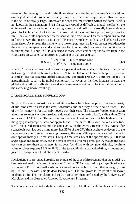
A calculation is presented here that are typical of the type of fire scenario that the model hasbeen re-designed to address. A snapshot from the FDS visualization package Smokeviewis shown in Fig. 2. A small cushion is ignited on a couch in a room that is roughly 5 mby 5 m by 2.5 m with a single door leading out. The fire grows to the point of flashoverin about 3 min. This simulation is based on an experiment performed by the University ofMaryland and the Bureau of Alcohol, Tobacco and Firearms.

The new combustion and radiation routines are crucial to this calculation because towards

832

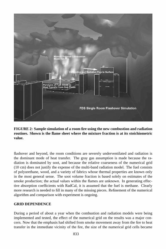
FIGURE 2: Sample simulation of a room fire using the new combustion and radiationroutines. Shown is the flame sheet where the mixture fraction is at its stoichiometricvalue.

flashover and beyond, the room conditions are severely underventilated and radiation isthe dominant mode of heat transfer. The gray gas assumption is made because the ra-diation is dominated by soot, and because the relative coarseness of the numerical grid(10 cm) does not justify the expense of the multi-band radiation model. The fuel consistsof polyurethane, wood, and a variety of fabrics whose thermal properties are known onlyin the most general sense. The soot volume fraction is based solely on estimates of thesmoke production; the actual values within the flames are unknown. In generating effec-tive absorption coefficients with RadCal, it is assumed that the fuel is methane. Clearlymore research is needed to fill in many of the missing pieces. Refinement of the numericalalgorithm and comparison with experiment is ongoing.

GRID DEPENDENCE

During a period of about a year when the combustion and radiation models were beingimplemented and tested, the effect of the numerical grid on the results was a major con-cern. Now that the emphasis had shifted from smoke movement away from the fire to heattransfer in the immediate vicinity of the fire, the size of the numerical grid cells became

833

more important. In many calculations that involve either relatively large spaces or rela-tively small fires, the grid resolution in the vicinity of the fire will be severely limited. Formany applications, this in itself may not be a problem since the fire merely serves as apoint source of heat and smoke. However, if one is interested in flame spread, near-fieldheat transfer is all-important, and the resolution of the numerical grid, especially during theearly stage of a fire, cannot be ignored.

We have found from various validation exercises involving pool fires and small compart-ments that good agreement with experimental data is possible when the fire is adequatelyresolved. However, even in cases where the fire is not well-resolved, it is possible to geta reasonable approximation of the total and radiative heat release rate of the fire, plus itsvolumetric distribution and flame height, with numerical grids that are very coarse. To dothis, one needs to slightly modify the procedure for obtaining the local heat release ratefrom the mixture fraction field. Note that this approximation is only intended for under-resolved fires. The above procedure for determining the local heat release rate works wellfor calculations in which the fire is adequately resolved.

What do we mean by “adequately resolved”? It depends on what the objective of thecalculation is. To a chemical kineticist, adequate resolution might involve micrometersand microseconds; to a fire dynamicist, millimeters and milliseconds; to a fire protectionengineer, meters and seconds. Arelativemeasure of how well a fire is resolved numericallyis given by the nondimensional expressionD∗/δx, whereD∗ is a characteristic fire diameter

D∗ =(

Qρ∞ cpT∞

√g

) 25

(13)

andδx is the nominal size of a grid cell. Note that the characteristic fire diameter is relatedto the characteristic fire size via the relationQ∗ = (D∗/D)5/2, whereD is the physicaldiameter of the fire. The quantityD∗/δx can be thought of as the number of computationalcells spanning the characteristic (not necessarily the physical) diameter of the fire. Themore cells spanning the fire, the better the resolution of the calculation. For fire scenarioswhereD∗ is small relative to the physical diameter of the fire, and/or the numerical grid isrelatively coarse, the stoichiometric surfaceZ = Zf will underestimate the observed flameheight [4]. It has been found empirically that a good estimate of flame height can be foundfor crude grids if a different value ofZ is used to define the combustion region

Zf ,effZf

= min

(1 , C

D∗

δx

)(14)

HereC is an empirical constant to be used for all fire scenarios. As the resolution ofthe calculation increases, theZf ,eff approaches the ideal value,Zf . The benefit of theexpression is that it provides a quantifiable measure of the grid resolution that takes intoaccount not only the size of the grid cells, but also the size of the fire.

A practical consideration when implementing this idea in the numerical model is that inmost casesD∗ is not known in advance if the fire is allowed to spread throughout a space.Somehow the quantityD∗/δx must be approximated based only on values of the fuel mass

834

FIGURE 3: Simulations of a 0.4 m by 0.4 m sand burner with progressively coarserresolution; from left to right, 2.5 cm, 5 cm, 10 cm and 20 cm grid cells.

flux, cell size, and mixture fraction near the burning surface. Assuming the actual firediameterD ∼ nδx wheren is the number of cells spanning the fire, it can be shown aftersubstituting terms that

D∗

δx∼ n4/5 Q∗ 2/5

local (15)

whereQ∗local is a quantity that resemblesQ∗, but it is defined locally

Q∗local =

q′′

ρ∞ cpT∞√

gδx(16)

Thenumber of cells spanningD∗, n, is not readily obtained in a calculation, but it has beenfound from numerous trials thatn is proportional to the maximum value ofZ in the gasphase cells of the numerical grid. In most practical calculations,Z is far less than its idealvalue of unity in the first gas phase grid cell above the burner due to the increased numericaldiffusion necessitated by the coarse grid.

Figure 3 shows the flame sheet from four simulations of a simple 0.4 m by 0.4 m propanesand burner set to 160 kW. The only difference between each is the grid resolution. Onlythe case with a 2.5 cm grid cell was run without need of the modified flame surface value.For the 5 cm case, the resolution factor was about 0.7, for the 10 cm case, the factor was 0.3,and for the 20 cm case the factor was about 0.1; all approximate since the factor fluctuatesslightly during the calculation. For propane,Zf = 0.06. Since the diffusion coefficient usedin the calculation is only of orderδx2, the flame surface in the 20 cm case would just barelyappear above the burner. An other way to look at it is that we are assuming fuel and oxygenburn instantaneously. The mixture fraction combustion model is equivalent to tracking

835

propane and oxygen through their respective transport equations and never allowing bothfuel and oxygen to exist in a single grid cell. As fuel emerges from the burner surface, it willmix with a disproportionately large amount of oxygen in the first grid cell adjacent to theburner. All of the heat of combustion will be liberated in that first grid cell, and the flameheight will be under-predicted. This phenomenon was noticed by Ma and Quintiere [4]who were doing some validation exercises involving flame height.

The adjustment of the flame surface is almost always necessary when the simulation startswith a small ignition source. It is usually impractical to provide a fine grid wherever the fireresides, since usually the fire will grow and spread. The benefit of the technique describedhere is that as the fire grows,D∗ grows, and the reliance on the adjusted flame sheet valuediminishes, and in many cases goes away entirely. For example, a flashed over room froma numerical point of view is a fire resolved with a numerical grid spanning the length andwidth of the room. However, during the initial growth stage, the fire may be supported byjust a few grid cells spanning the width of the small fire. Of course, there are techniquesused in various fields of CFD to apply fine grids to where they are needed, even adjustingthe grids during a calculation. This latter technique, adaptive grid refinement, is difficultto apply and increases the cost of the calculation significantly. A more modest technique,known as multi-block, allows the user to specify grids of various refinement throughout thecomputational domain. Its practical application would be to finely grid a room of origin ina building, and use a coarser grid elsewhere. Such an effort is underway at NIST, but nomatter how well it works, there will probably always be a need to model a relatively smallfire on a relatively coarse grid.

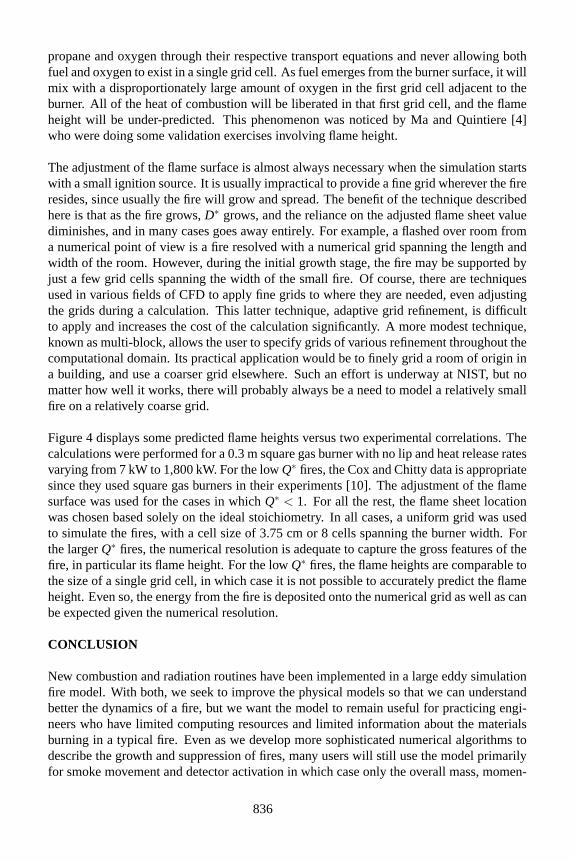
Figure 4 displays some predicted flame heights versus two experimental correlations. Thecalculations were performed for a 0.3 m square gas burner with no lip and heat release ratesvarying from 7 kW to 1,800 kW. For the lowQ∗ fires, the Cox and Chitty data is appropriatesince they used square gas burners in their experiments [10]. The adjustment of the flamesurface was used for the cases in whichQ∗ < 1. For all the rest, the flame sheet locationwas chosen based solely on the ideal stoichiometry. In all cases, a uniform grid was usedto simulate the fires, with a cell size of 3.75 cm or 8 cells spanning the burner width. Forthe largerQ∗ fires, the numerical resolution is adequate to capture the gross features of thefire, in particular its flame height. For the lowQ∗ fires, the flame heights are comparable tothe size of a single grid cell, in which case it is not possible to accurately predict the flameheight. Even so, the energy from the fire is deposited onto the numerical grid as well as canbe expected given the numerical resolution.

CONCLUSION

New combustion and radiation routines have been implemented in a large eddy simulationfire model. With both, we seek to improve the physical models so that we can understandbetter the dynamics of a fire, but we want the model to remain useful for practicing engi-neers who have limited computing resources and limited information about the materialsburning in a typical fire. Even as we develop more sophisticated numerical algorithms todescribe the growth and suppression of fires, many users will still use the model primarilyfor smoke movement and detector activation in which case only the overall mass, momen-

836

FIGURE 4: Comparison of predicted flame heightsversus Heskestad’s correlation (solid line) [11] andCox and Chitty’s (dashed line) [10].

tum and energy transport from the fire is needed. The objective of the model developmentis to make it as useful as possible for a wide variety of applications, both fundamentaland applied. If successful, the model will be exercised by a large variety of users whicheliminates computer bugs, introduces field modeling to a new generation of fire protectionengineers, and most importantly provides validation of the algorithms for a wide variety ofexperimental data sets. This is an evolving process. Work still needs to be done in manyareas, especially soot production, radiation absorption coefficients, numerical resolution,and material properties. Progress will be made because of better research in the future, butalso because of lessons learned from calculations being performed now. The developmentof zone models over the past few decades certainly benefited from the wide use of the earlymodels, pointing out both the strengths and weaknesses, and ultimately guiding the devel-opment of newer algorithms. The same will be true of field models if the proper balance isstruck between research and practical application.

ACKNOWLEDGEMENTS

The authors would like to thank Drs. Paul Fuss and Anthony Hamins for their assistancewith the radiation absorption coefficients.

837

REFERENCES

[1] K.B. McGrattan, H.R. Baum, R.G. Rehm, A. Hamins, and G.P. Forney. Fire Dynam-ics Simulator, Technical Reference Guide. Technical Report NISTIR 6467, NationalInstitute of Standards and Technology, Gaithersburg, Maryland, January 2000.

[2] K.B. McGrattan and G.P. Forney. Fire Dynamics Simulator, User’s Manual. TechnicalReport NISTIR 6469, National Institute of Standards and Technology, Gaithersburg,Maryland, January 2000.

[3] S. Hostikka, H.R. Baum, and K.B. McGrattan. Large Eddy Simulations of the ConeCalorimeter. InProceedings of US Section Meeting of the Combustion Institute, Oak-land, California, March 2001.

[4] T. Ma. Numerical Simulation of an Axi-symmetric Fire Plume: Accuracy and Limi-tations. Master’s thesis, University of Maryland, 2001.

[5] S. Hostikka and K.B. McGrattan. Large Eddy Simulations of the Wood Combustion.In Interflam 2001, Proceedings of the Ninth International Conference. InterscienceCommunications, 2001.

[6] J.E. Floyd, C. Wieczorek, and U. Vandsburger. Simulations of the Virginia Tech FireResearch Laboratory Using Large Eddy Simulation with Mixture Fraction Chemistryand Finite Volume Radiative Heat Transfer. InInterflam 2001, Proceedings of theNinth International Conference. Interscience Communications, 2001.

[7] C. Huggett. Estimation of the Rate of Heat Release by Means of Oxygen Consump-tion Measurements.Fire and Materials, 4:61–65, 1980.

[8] W. Grosshandler. RadCal: A Narrow Band Model for Radiation Calculations in aCombustion Environment. NIST Technical Note (TN 1402), National Institute ofStandards and Technology, Gaithersburg, Maryland 20899, 1993.

[9] H. Koseki and T. Yumoto. Air Entrainment and Thermal Radiation from HeptanePool Fires.Fire Technology, 24, February 1988.

[10] G. Cox and R. Chitty. Some Source-Dependent Effects on Unbounded Fires.Com-bustion and Flame, 60:219–232, 1985.

[11] B.J. McCaffrey. SFPE Handbook, chapter Flame Height. National Fire ProtectionAssociation, Quincy, Massachusetts, 2nd edition, 1995.

838