In This Lecture We Begin the Study

7/17/2019 In This Lecture We Begin the Study

http://slidepdf.com/reader/full/in-this-lecture-we-begin-the-study 1/12

LECTURE 7: FIRST-ORDER ODES

In this lecture we begin the study of ordinary differential equations (ODEs) by deriving themfrom physical or other problem (modeling ), solving them by standard mathematical methods,and interpreting solutions and their graphs in terms of a given problem. The simplest ODEs tobe discussed are ODEs of the first order because they involve only the first derivative of theunknown function and no higher derivatives. These unknown functions will usually be denoted byy(x) or y(t) when the independent variable denotes time t .

Understanding the basics of ODEs requires solving problems by hand (paper and pencil). Indoing so, you will gain an important conceptual understanding and feel for the basic terms, suchas ODEs, direction field, and initial value problem.

Figure 1. Modeling, solving, interpreting

1. Basic Concepts of ODEs

If we want to solve an engineering problem (usually of a physical nature), we first have toformulate the problem as a mathematical expression in terms of variable, functions, and equations.

Such an expression is known as a mathematical model of the given problem. The process of setting up a model, solving it mathematically, and interpreting the result in physical or other termsis called mathematical modeling or, briefly, modeling.

Modeling needs experience, which we shall gain by discussing various examples and problems.Now many physical concepts, such as velocity and acceleration, are derivatives. Hence a model

is very often an equation containing derivatives of an unknown function. Such a model is called adifferential equation. Of course, we then want to find a solution (a function that satisfies theequation), explore its properties, graph it, find values of it, and interpret it in physical terms sothat we can understand the behavior of the physical system in our given problem. However, before

1



2 LECTURE 7: FIRST-ORDER ODES

Figure 2. Some applications of differential equations



LECTURE 7: FIRST-ORDER ODES 3

we can turn to methods of solution, we must first define some basic concepts needed throughoutthis lecture.

An ordinary differential equation (ODE) is an equation that contains one or several deriva-tives of an unknown function, which we usually call y(x) (or sometimes y(t) if the independent vari-able is time t. The equation may also contain y itself, known functions of x (or t ), and constants.For example,

y = cos x (1.1)

y + 9y = e−2x (1.2)

yy − 3

2y2 = 0 (1.3)

are ordinary differential equations (ODEs). Here, as in calculus, y denotes, y denotes dy/dx,y = dy2/dx2, etc. The term ordinary distinguishes them from partial differential equation (PDEs),which involve partial derivatives of an unknown function of two or more variables. For instance, aPDE with unknown function u of two variables x and y is

∂ 2u

∂x2 +

∂ 2u

∂y 2 = 0,

called Laplace equation, which is satisfied by the real and imaginary part of the analytic complexfunctions. PDEs have important engineering applications, but they are more complicated thanODEs.

An ODE is said to be of order n if the nth derivative of the unknown function y is the highestderivative of y in the equation. The concept of order gives a useful classification into ODEs of firstorder, second order, and so on. Thus, (1.1) is of first order, (1.2) of second order, and (1.3) of thirdorder.

In this lecture we shall consider first-order ODEs. Such equation contain only the first deriv-ative y and may contain y and any given function of x. Hence we can write them as

F (x,y,y) = 0, (implicit form)

or often in the formy = f (x, y). (explicit form)

For instance, the implicit ODE x−3y−4y2 = 0 (where x = 0) can be written explicitly as y = 4x3y2.

2. Concept of Solution

A function

y = h(x)

is called a solution of a given ODE F (x,y ,y) = 0 on some open interval a < x < b if h(x) isdefined and differentiable throughout the interval and is such that the equation becomes an identityif y and y are replaced with h and h, respectively. The curve (the graph) of h is called a solutioncurve.

Example 1. (A) Exponential Growth. (B) Exponential Decay (A) From calculus we know that y = ce0.2t has the derivative

y = dy

dx = 0.2e0.2t = 0.2y.

Hence y is a solution of y = 0.2y (Fig. 3 A). This ODE is of the from y = ky. With positive-constant k it can model exponential growth, for instance, of colonies of bacteria or populations of animals. It also applies to humans for small populations in a large country (e.g. the China in early times) and is then known as Malthus’s law.




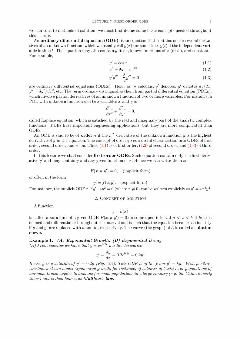
(B) Similarly, y = −0.2y (with a minus on the right) has the solution y = ce−0.2t, (Fig. 3 B)modeling exponential decay. as, for instance, of a radioactive substance (see Example 5).

Figure 3. Exponential Growth and Decay

We see that each ODE in these example has a solution that contain an arbitrary constant c.Such a solution containing an arbitrary constant c is called a general solution of the ODE.

Geometrically, the general solution of an ODE is a family of infinitely many solution curves,one for each value of the constant c. If we choose a specific c (e.g., c = 6.45 or 0 or −2.01) weobtain what is called a particular solution of the ODE. A Particular solution does not containany arbitrary constants.

3. Initial Value Problem

In most cases the unique solution of a given problem, hence a particular solution, is obtainedfrom a general solution by an initial condition y(x0) = y0, with given values x0 and y0, that isused to determine a value of the arbitrary constant c. Geometrically this condition means that thesolution curve should pass through the point (x0, y0) in the xy-plane. An ODE, together with aninitial condition, is called an initial value problem. Thus, if the ODE is explicit, y = f (x, y),the initial value problem is of the form

y = f (x, y), y(x0) = y0

Example 2. Radioactivity. Exponential Decay Given an amount of a radioactive substance, say. 0.5g (gram), find the amount present at any later time.

Physical Information. Experiments show that at each instant a radioactive substance decomposes-and is thus decaying in time-proportional to the amount of substance present.Step 1. Setting up a mathematical model of the physical process. Denotes by y(t) the amount of substance still present at any time t. By the physical law, the time rate of change y(t) = dy/dt is proportional to y(t). This gives the first-order ODE

dy

dt = −ky

where the constant k is positive, so that, because of the minus, we do get decay. The value of k is known from experiments for various radioactive substances (e.g., k = 1.4 ·10−11s−1, approximately,




for radium 22688Ra). Now the given initial amount is 0.5g, and we can call the corresponding instant

t = 0. Then we have the initial condition y(0) = 0.5. This is the instant at which our observation of the process begins. It motivates the term initial condition. Hence the mathematical model of the physical process is the initial value problem

dy

dt

=

−ky, y(0) = 0.5

Step 2. Mathematical solution. This ODE models exponential decay and has the general solution (with arbitrary constant c but definite given k)

y(t) = ce−kt.

We now determine c by using the initial condition. Since y(0) = c, this gives y(0) = c = 0.5. Hence the particular solution governing our process is

y(t) = 0.5e−kt (k > 0).

Step 3. Interpretation of result. This formula gives the amount of radioactive substance at time t. It starts from the correct initial amount and decrease with time because k is positive. The limit of y as t →∞ is zero (Fig. 4).

Figure 4. Radioactivity

4. Separable ODEs

Many practically useful ODEs can be reduce to the form

g(y)y = f (x) (4.1)

by purely algebraic manipulations. Then we can integrate on both sides with respect to x, obtaining g(y)ydx =

f (x)dx + c.

On the left we can switch to y as the variable of integration. By calculus, ydx = dy, so that

g(y)dy =

f (x)dx + c.

If f and g are continuous functions, the integrals exist, and by evaluating them we obtain a generalsolution (4.1). This method of solving ODEs is called the method of separating variables, and(4.1) is called aseparable equation.

Example 3. Separable ODE The ODE y = 1 + y2 is separable because it can be written

dy

1 + y2 = dx. By integration, arctan y = x + c or y = tan(x + c)




It is very important to the constant of integration immediately when the integration is performed. If we wrote arctan y = x, then y = tan x, and then introduced c, we would have obtained y = tan x + c,which is not a solution (when c = 0 ). Verify this.

Example 4. Separable ODE The ODE y = (x + 1)e−xy2 is separable; we obtain y−2dy = (x + 1)e−xdx. By integration,

−y−1

= −(x + 2)e−x

+ c. y = 1

(x+2)e−x−c

Example 5. Initial Value Problem (IVP). Bell-Shaped CurveSolve y = −2xy, y(0) = 1.8.Solution. By separation and integration

dy

y = −2xdx, ln y = −x2 + c, y = ce−x2.

This is the general solution. From it and the initial condition, y(0) = ce0 = c = 1.8. Hence the

IVP has the solution y = 1.8e−x2 . This is a particular solution, representing a bell-shaped curve (Fig. 5 ).

Figure 5. Bell-shaped curve

5. Modeling

We know that modeling is very important. Separable equations yield various useful models. Letus discuss this in terms of some typical examples.

Example 6. Radiocarbon Dating In September 1991 the famous Iceman (Oetzi), a mummy from the Neolithic period of the Stone Age found in the ice of the Oetztal Alps (hence the name “Oetzi”) in Southern Tyrolia near the Austrian-Italian border, caused a scientific sensation. When did Oetzi approximately live and die if the ratio of carbon 14

6C to carbon 126C in this mummy is 52.5% of that of a living organism?

Physical information. In the atmosphere and in living organisms, the ratio of radioactive car-

bon 14

6C (made radioactive by cosmic rays) to ordinary carbon 12

6C is constant. When an organism dies, its absorption of 146C by breathing and eating terminates. Hence one can estimate the age of

a fossil by comparing the radioactive carbon ratio in the fossil with that in the atmosphere. To dothis, one needs to know the half-life of 14

6C, which is 5715 years (CRC Handbook of Chemistry andPhysics, 83rd, Boca Raton: CRC Press, 2002, page 11-52, line 9).

Solution. Modeling Radioactive decay is governed by the ODE y = ky. By separation and integration (where t is time and y0 is the initial ratio of 14

6C to 126C )

dy

y = kdt, ln |y| = kt + c, y = y0ekt (y0 = ec).




Next we use the half-life H = 5715 to determine k. When t = H , half of the original substance is still present. Thus,

y0ekH = 0.5y0, ekH = 0.5, k = ln 0.5

H = −0.693

5715 = −0.0001213.

Finally, we use the ratio 52.5% for determining the time t when Oetzi died (actually, was killed),

ekt = e−0.0001213t = 0.525, t = ln 0.525−0.0001213

= 5312. Answer : About 5300 years ago.

Other methods show that radiocarbon dating values are usually too small. According to recent research, this is due to a variation in that carbon ratio because of industrial pollution and other factors, such as nuclear testing.

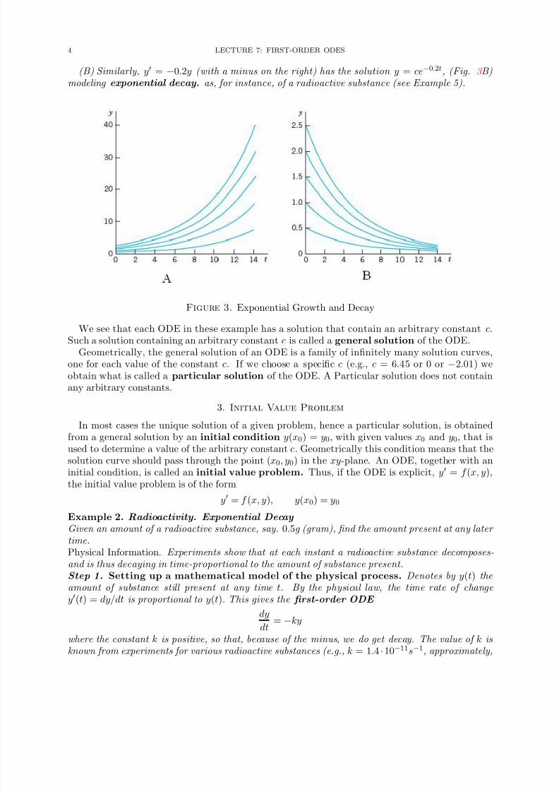
Example 7. Mixing Problem Mixing problems occur quite frequently in chemical industry. We explain here how to solve the basic model involving a single tank. The tank in Fig. 6 contains 1000 gal of water in which initially 100 lb of salt is dissolved. Brine runs in at a rate of 10 gal/min, and each gallon contains 5 lb of dissolved salt. The mixture in the tank is kept uniform by stirring. Brine runs out at 10 gal/min.Find the amount of salt in the tank at any time t.

Figure 6. Mixing problem

Solution. Step 1. Setting up a model. Let y(t) denote the amount of salt in the tank at time t. Its time rate of change is

y = Salt inflow rate − Salt outflow rate Balance law.

5 lb times 10 gal gives an inflow of 50 lb of salt. Now, the outflow is 10 gal of brine. This is 10/1000=0.01 (=1%) of the total brine content in the tank, hence 0.01 of the salt content y(t).Thus the model is the ODE

y = 50 − 0.01y = −0.01(y − 5000).

Step 2. Solution of the model. The ODE is separable. Separation, integration, and taking exponents on both sides gives

dy

y − 5000 = −0.01dt, ln |y − 5000| = −0.01t + c∗

, y − 5000 = ce−

0.01t.

Initially the tank contains 100 lb of salt. Hence y (0) = 100 is the initial condition that will give the unique solution, Substituting y = 100 and t = 0 in the last equation gives 100 − 5000 = ce0 = c.Hence c = −4900.

y(t) = 5000 − 4900e−0.01t.

This function shows an exponential approach to the limit 5000 lb; see Fig. 6 . Can you explain physically that y(t) should increase with time? That its limit is 5000 lb? Can you see the limit directly from the ODE?




The model discussed becomes more realistic in problems on pollutants in lakes or drugs in organs.These types of problems are more difficult because the mixing may be imperfect and the flow rates (in and out) may be different and known only very roughly.

Example 8. Leaking Tank. Outflow of Water Through a Hole (Torricelli’s Law)This is another prototype engineer problem that leads to an ODE. It concerns the outflow of water

from a cylindrical tank with a hole at the bottom (Fig. 7 ). You are asked to find the height of the water in the tank at any time if the tank has diameter 2 m, the hole has diameter 1 cm, and the initial height of the water when the hole is opened is 2.25 m. When will the tank be empty?

Physical information. Under the influence of gravity the out flowing water has velocity

v(t) = 0.600

2gh(t) (Torricelli’s law )

where h(t) is the height of the water above the hole at time t, and g = 980cm/s2 = 32.17ft/s2 is the acceleration of gravity at the surface of the earth.

Solution. Step 1. Setting up the model. To get an equation, we relate the decrease in water level h(t) to the outflow. The volume ∆V of the outflow during a short time ∆t is

∆V = Av ∆t (A = Area of hole)

∆V must equal the change ∆V ∗ of the volume of the water in the tank. Now

∆V ∗ = −B ∆h (B = Cross− sectional area of tank)

where ∆h (> 0) is the decrease of the height h(t) of the water. The minus sign appears because the volume of the water in the tank decreases. Equating ∆V and ∆V ∗ gives

−B∆h = Av ∆t.

We now express v according to Torricelli’s law and then let ∆t approach 0–this is a standard way of obtaining an ODE as a model. That is, we have

∆h

∆t = −A

Bv = −A

B0.600

2gh(t)

and by letting ∆t → 0 we obtain the ODE.

dh

dt = −26.56

A

B

√ h,

where 26.56 = 0.600√

2 · 980. This is our model, a first-order ODE.Step 2. General solution. Our ODE is separable. A/B is constant. Separation and integra-

tion gives dh√

h= −26.56

A

Bdt and 2

√ h = c∗ − 26.56

A

Bt.

Dividing by 2 and squaring gives h = (c−13.28At/B)2. Inserting 13.28A/B = 13.28·0.52π/1002π =0.000332 yields the general solution

h(t) = (c − 0.000332t)2.

Step 3. Particular solution. The initial height (the initial condition) is h(0) = 225cm.Substitution of t = 0 and h = 225 gives from the general solution c2 = 225, c = 15.00 and thus the particular solution (Fig. 7 )

h p(t) = (15.00 − 0.000332t)2.

Step 4. Tank empty. h p(t) = 0 if t = 15.00/0.000332 = 45, 181 [sec] = 12.6[hours]. Here you see distinctly the importance of the choice of units




Figure 7. Leaking tank

6. Linear first-order ODEs

Linear ODEs or ODEs that can be transformed to linear form are models or various phenomena,for instance, in physics, biology, population dynamics, and ecology as we shall see. A first-orderODE is said to be linear if it can be bought into the form

y + p(x)y = r(x) (6.1)

by algebra, and nonlinear if it cannot be bought into this form.The defining feature of this linear ODE is that it is linear in both the unknown function y and its

derivative y , whereas p and r may be any given functions of x. If in an application the independentvariable is time, we write t instead of x.

If the first term is f (x)y (instead of y ), divide the equation by f (x) to get the standard form,

with y

as the first term, which is practical.For instance, y cos x+y sin x = x is a linear ODEs, and its standard form is y +y tan x = x sec x.The function r(x) on the right way be a force, and the solution y (x) a displacement in a motion

or an electrical current or some other physical quantity. In engineering, r(x) is frequently calledthe input, and y(x) is called the output or the response to the input (and, if given, to the initialcondition).

We now solve the linear ODE (6.1) in the interval J considered. In what follows, we look for afunction F (x), called integrating factor. Multiplying (6.1) by F (x), we obtain

F y + pF y = rF.

If

pF y = F

y, i.e. pF = F

,the left side is the derivative (F y) = F y + F y of the product F y. By separating variables,dF/F = pdx. By integration, writing h =

pdx,

ln |F | = h =

pdx, thus F = eh.

With this F and h = p, we have

ehy + hehy = ehy + (eh)y = (ehy) = reh.




By integration,

ehy =

ehrdx + c.

Dividing by eh, we obtain the desired solution formula

y(x) = e−h( ehrdx + c), h = p(x)dx.

This reduces solving (6.1) to the generally simpler task of evaluating integrals.The structure of the solution is interesting. The only quantity depending on a given initial

condition is c. Accordingly, writing the solution as a sum of two terms.

y(x) = e−h

ehrdx + ce−h,

we see the following:

Total Output = Response to the Input r + Response to the Initial Data.

Example 9. Electric Circuit

Model the RL-circuit in Fig .8 and solve the resulting ODE for the current I (t) A (amperes),where t is time. Assume that the circuit contains as an EMF E (t) (electromotive force) a battery of E = 48V (volts), which is constant, a resistor of R = 11Ω (ohms), and an inductor of L = 0.1H (henrys), and that the current is initially zero.

Figure 8. RL-circuit

Physical Laws. A current I in the circuit causes a voltage drop RI across the resistor ( Ohm’s law ) and a voltage drop LI = LdL/dt across the conductor, and the sum of these twovoltage drops equals the EMF ( Kirchhoff’s Voltage Law, KVL).

Solution. According to these laws the model of the RL-circuit is LI + RI = E (t), in standard form

I + RL

I = E (t)L

.

We can solve this linear ODE, obtaining the general solution

I = e−(R/L)t(

e(R/L)t E (t)

L dt + c).

By integration,

I = e−(R/L)t(E

L

e(R/L)t

R/L + c) =

E

R + ce−(R/L)t.




In our case, R/L=11/0.1=110 and E (t)=48/0.1=480=const; thus,

I = 48

11 + ce−110t.

The initial value I (0) = 0 gives I (0) = E /R + c = 0,c = −E/R and the particular solution

I =

E

R (1 − e−(R/L)t

), thus I =

48

11 (1 − e−110t

).

7. problems

(1) Solve the first-order ODEs.(a) y3y + x3 = 0,(b) y = e2x−1y2,(c) xy = x + y (set y/x = u)(d) xy + y = 0, y(4) = 6,(e) y = (x + y − 2)2, y(0) = 2 (set v = x + y − 2),(f) xy = y + 3x4 cos2(y/x), y(1) = 0 (set y /x = u).

(2) Find the general solution. If an initial condition is given, find also the correspondingparticular solution(a) y + ky = e−kx,(b) xy = 2y + x3ex,(c) y − ny/x = −xn−2 cos(1/x),(d) y + y = y2, y(0) = −1

3 ,

(e) y = (tan y)/(x − 1), y(0) = 12 π.

(3) Exponential decay. Subsonic flight. The efficiency of the engines of subsonic airplanesdepends on air pressure and is usually maximum near 35, 000 ft. Find the air pressurey(t) at this heigh. Physical information. The rate of change y(x) is proportional to thepressure. At 18, 000 ft it is half its value y0 = y(0) at sea level. Hint. Remembering fromcalculus without calculation that the answer should be close to y0/4?

(4) Boyle-Mariotte’s law for ideal gases. Experiments show for a gas at low pressure p

(and constant temperature) the rate of change of the volume V ( p) equals −V /p. Solve themodel.(5) Friction. If a body slides on a surface, it experiences friction F (a force against the

direction of motion). Experiments show that |F | = µ|N | (Coulomb’s law of kinetic friction without lubrication ), where N is the normal force (force that holds the two surfaces togetherand the constant of proportionality µ is called the coefficient of kinetic friction . In Fig. 9assume that the body weighs 45 nt. µ = 0.20 (corresponding to steel on steel). a = 30,the slide is 10 m long, the initial velocity is zero, and air resistance is negligible. Find thevelocity of the body at the end of the slide.

Figure 9. Friction




(6) A Riccai equation is of the form

y + p(x)y = g(x)y2 + h(x).

(a) Apply the transformation y = Y + 1/u to the Riccati equation, where Y is a solution of the Riccati equation, and obtain for u the linear ODE u + (2Y g − p)u = −g. Explainthe effect of the transformation by writing it as y = Y + v, v = 1/u.

(b) Show that y = Y = x is a solution of the ODE y − (2x3 + 1)y = −x2y2 − x4 − x + 1

and solve this Riccati equation, showing the details.(7) Air circulation. In a room containing 20000 ft3 of air, 600 ft3 of fresh air flows in per

minute, and the mixture (made practically uniform by circulating fans) is exhausted at arate of 600 cubic feet per minute(cfm). What is the amount of fresh air y (t) at any time if y(0) = 0? After what time will 90% of the air be fresh?

(8) Hanging cable. It can be shown that the curve y(x) of an inextensible flexible homogenous

cable between two fixed points is obtained by solving y = k

1 + y2, where the constantk depends on the weight. This curve is called catenary (from Latin catena=the chain).Find and graph y(x), assuming that k = 1 and those fixed points are (−1, 0) and (1, 0) ina vertical xy-plane.

Documents

In This Lecture We Begin the Study