Indian Sensitive Index (Sensex) and Assets Pricing ...Indian Sensitive Index (Sensex) and Assets Pricing Literature in Financial Economics 7 The rest of the paper is organized as follows:

The IUP Journal of Financial Economics, Vol. IV, No. 2, 20066

Indian Sensit ive Index (Sensex)and Assets Pricing Literature

in Financial Economics

Capital Asset Pricing Model (CAPM) rel ies heavily on the stock market indexas it is practical ly impossible to collect the entire data from the complexstock market. Though beta value is derived by applying such indices,empir ical findings and conclusions vary from one finding to another. This paperbriefly presents such findings under four broad headings. The first one gives aconcise view of early development of CAPM when beta is considered—before1980s—the messiah to pr icing of an asset. In the 1980s and 1990s, someresearchers concluded that many other variables also influence the assetpr icing model and declared beta dead. The second heading presents theanomalies or puzzles in CAPM. After the 1990s, some researchers asserted thatasset pr icing is pr imarily based on behavioral atti tude of investors. This is dealtwith under the third heading CAPM, the sui gener is. The collaged Indianempir ical findings on CAPM are presented under the last part.

© 2006 IUP. All Rights Reserved.

A Peer Mohamed*

* Senior Lecturer, School of Accounting and Finance, Binary University College, Bandar Puchong Jaya,47100 Selangor, West Malaysia. E-mail: [email protected]

1. Introduction

Sensex is regarded to be the pulse of the Indian stock market. History is created at the fagend of the session at around 3:12 pm on February 6, 2006 when Sensex crossed the 10,000level and reached 10,002.83, the day’s high, before closing at 9,980.42. This is a milestonefor the Indian capital markets. It reflects the underlying strength of the economy and the leapof faith that global and local investors have taken on India.

Sensex depicts market index. For asset pricing, market index is the base to create �E.When market index moves, the value of a stock also moves in tandem with the market index.Increase in market price leads to increase in share price and ultimately increase in marketcapitalization. The Capital Asset Pricing Model (CAPM) theoretically depends on wholemarket such as share market, money market, antique/painting market, human capital market,etc. As practically it is not worth to collect data for the whole market, CAPM relies heavilyon stock market index. Our market index (Sensex) is robust now. We are, therefore, forcedto know the literature on CAPM. This paper surveys and reviews the field of assets pricingliterature and the emphasis is on the interplay between theory and empirical work.

7Indian Sensitive Index (Sensex) and Assets Pricing Literature in Financial Economics

The rest of the paper is organized as follows:

• Early Development of the Capital Asset Pricing Model (a concise view is given);

• Anomalies in the CAPM (theorists develop models with testable predictions, but there arestylized facts that fail to fit established theories, called “puzzles”, these puzzles aresurveyed here);

• The sui generis CAPM (a brief view of application of behavioral science on the CAPM);

• Indian Empirical Findings on the CAPM; and

• Conclusion.

2. Early Developments of CAPM

The first shareholder-owned business might be the Dutch East India Company, with an objectof trading with India, was founded by Dutch Merchants in 1602 and issued negotiable sharecertificates that were readily traded in Amsterdam until the company failed almost twocenturies later. By the 17th Century, traders in London coffee houses earned their livingdealing in the shares of joint-stock companies. But it was not until the industrial revolutionmade it necessary to raise large amount of capital to build factories and canals that sharetrading became widespread. In the 20th century, the world stock market moved towards itszenith. The gigantic growth of stock market results into the capitalization of world’s stockmarkets in 2005 as $39 tn. CAPM becomes workable horse for stock market.

The Three Ps

There are three Ps that are directly related to share prices and their behavior, namely,“Preferences, Probability and Price”1. Formal models of asset prices and financial markets,such as those of Merton (1973), Lucas (1978), Breeden (1979) and Cox, Ingersoll, and Ross(1985), show precisely how the three Ps simultaneously determine an “equilibrium” in whichdemand equals supply across all markets in an uncertain world. For example, given anequilibrium in which preferences and probabilities are specified, prices are determined exactly(this is the central focus of the asset pricing literature in economics).

Preferences

Preference of an asset can be directly expressed in terms of utility. In the framework proposedby Von Neumann and Morganstern and Savage, any individual’s preferences can berepresented numerically by a utility function U (X) under certain axioms.2 In other words, ifan individual’s preferences satisfy these axioms then a utility function U (X) can beconstructed in such a way that the individual’s choices among various alternatives willcoincide with the choices that maximize the individual’s expected utility, E[U(X)]. This utilityfunction can be traced back to St. Petersburg Paradox.

An individual is offered this gamble: “A fair coin is tossed until it comes up heads, atwhich point the individual is paid a prize of $2k, where k is the number of times the coinis tossed.” How much should an individual pay for such a gamble?

The expected value of this gamble is infinite, yet individuals are typically willing to payonly between $2 and $4 to play. And this is the St. Petersburg’s Paradox. Why are they willingto pay only between $2 and $4?


Daniel Bernoulli (1738) resolves the Paradox by asserting that gamblers do not focus onthe expected gain of a wager but, rather, they focus on the expected logarithm of the gain,in which case, the “value in use” of St. Petersburg gamble is:

42log2)2(log21

� � ��

� �¦�f

...(1)

Although Bernoulli does not present his resolution of the St. Petersburg Paradox in termsof utility, the essence of his proposal is to replace expected value as a gambler’s objectivewith expected utility, where utility is defined to be the logarithm of gain. This approach todecision-making under uncertainty is remarkably prescient;

The price, Pt, of any financial security that pays a stream of dividends D

t+1, D

t+2,... must

satisfy the following relationship:

�»�¼

�º�«�¬

�ª�c

�f� ��

��

� �¦ �W

�W�W

�W

...(2)

where, U't(C

t) and U'

t+�W (Ct+�W) are marginal utilities of consumption at dates

t and

t+�W,

respectively. This “maximizing the expected utility E[U(X)]” is a powerful representation. Itlies at the heart of virtually every modern approach to pricing financial assets, includingmodern portfolio theory, mean-variance optimization, the Capital Asset Pricing Model, theInter-temporal CAPM, and the Cox-Ingersoll-Ross (1985) term-structure model.

Pr obabil i ty

Objective (or statistical/aleatory) probabilities are based on the notion of relative frequencies

in repeated experiments. On the other hand, subjective (or personal/epistemic) probabilities

measure “degree of belief”, which is not based on statistical phenomena. The link between

subjective probabilities and risk management becomes even stronger when considered in light

of the foundations on which subjective probabilities are built. The three main architects ofthis theory—Ramsey (1926), De Finetti (1937), and Savage (1954)—argue that, despite the

individualistic nature of subjective probabilities, they must still satisfy the same mathematical

laws as objective probabilities; otherwise, objective probabilities will arise. Subjective

probabilities behave like objective probabilities in every respect. This principle is often called

“Dutch book theorem.”3

Pr ice

Equilibrium is a function of price. Price, probability and preferences or utility are interlacedwith each other. One of the great successes of modern economics is the sub-field known asasset pricing; within asset pricing, surely the crowning achievement is the development ofprecise mathematical models for pricing and hedging derivative securities. The basic equationof asset pricing can be written as follows:4

Pit = E

t [M

t+1 X

i, t+1] ...(3)


where, Pit is the price of an asset I at time t (“today”), E

t is the conditional expectations

operator conditioning on today’s information, Xi, t+1

is the random payoff on asset I at timet + 1 (“tomorrow”) and M

t+1 is the Stochastic Discount Factor (SDF). The SDF is a random

variable whose realizations are always positive. According to the standard present valuerelationship, the fundamental real price of an asset at time t is5:

�»�¼

�º�«�¬

�ª�¸�¸�¹

�·�¨�¨�©

�§� ��

� ��

�f

� �–�¦ it

j

1i1t

1jt

ft ��!EP ...(4)

where, Et [.] denotes the mathematical expectation conditional on all information available

at time t, and �T��refers to the accumulated real dividend or other payoff on the asset from timet–1 through t. Finally the discount factor is �U

t�{ exp (–r

t), where r

t is a continuously

compounded required rate of return.

The Beginning of Investment Theory

The vertex of the study of capital assets starts earlier exactly 105 years from now by a Frenchmathematician Louis Bachelier (1990) in his Ph.D thesis about ‘random walk’ hypothesis. Heuses Brownian motion as a model for stock exchange performance. He is the first to applythe trajectories of Brownian motion, and his theories prefigure modern mathematical finance.Constructs developed by Kenneth Arrow and Gerard Debreu provided a similar foundation forfinancial economics. Their approach represents securities and other types of financialinstruments in terms of their most elemental components.

Markowitz’s Efficient Frontier

Statistical analysis is made on stock prices. John Burr Williams (1938) is the first man toobserve that subjective probabilities should be assigned to various possible values of securityand the mean of these values is used as the value of security. “In the end all prices dependon someone’s estimate of future income”. This statement, taken from John Burr Williams’ 1938text, pierces the very heart of the subject of finance. Yet his stance is atypical, and in generalthe economic-theory-based approach he adopts was remarkably modern. He further observesthat by investing in sufficiently many securities, risk could be virtually eliminated. Leavens(1945) further suggest diversification among industries is needed to protect againstunfavorable factors.

These publications, unfortunately, lack risk-return trade-off, correlation of securities’weights, covariance between securities and utility theory. Preference or utility is the motivebehind consumption and investment. Markowitz (1952) synthesized all the parameters andgeometrically developed Investment Theory, based on the probabilistic notion of expectedreturn and risk.

His work is based on the idea that stock returns are normally distributed and that peoplelike returns and do not like risk. Thus they want high mean, low standard deviation portfolio.The portfolios that have the highest return for a given level of risk are called theMean-Variance Efficient frontier (MVE). When we graph the efficient portfolios in risk-returnspace the concave line is the ‘efficient frontier’.


Risk can be broken into market (systematic/undiversifiable) risk and unique (firm-specific/diversifiable/unsystematic/idiosyncratic) risk. Diversified investors are concerned with marketrisk. Beta is an asset’s contribution to the risk of a fully diversified portfolio. Beta iscalculated by regressing the asset’s return against the market portfolio. Thus the beta ofTreasury Bills is zero and the beta of the market portfolio is 1.00.

The Capital Asset Pr icing Model

A homogeneous expectation is an assumption in the Capital Asset Pricing Model (CAPM) thatstates that all investors see the same risk-return profile for assets. Investor’s risk toleranceinteractions for risky alternatives, in competitive markets, provide signals to the economy inthe form of asset prices. This valuation of risky assets results in an efficient allocation ofresources in the economy over time.

The CAPM shows that the equilibrium rate of return on a risky asset is a linear functionof its covariance with the market portfolio; it can be expressed in terms of a simple linearmodel that captures the trade-off between the firm’s expected returns and expected systematic(non-diversifiable) risk. In its ex ante form it can be represented by:

E (Rt) = R

ft + �E(R mt– ft

.. (5)

where, E (Rt) is the ex ante expected returns of a firm, R

ft is the contemporaneous

risk-free rate, �Ei is the systematic risk of a firm and R

mt is the return on the market portfolio.

The Empir ical CAPM

The CAPM is an equilibrium model and the relationship between beta and expected returnis explicitly specified, but it does not mention the empirical way of testing the CAPM.Expected return rests on the expectations of the investors, which is ex ante and it cannot beascertained so easily. Hence, a researcher is left with the only chance of testing the CAPMwith ex post returns data. We need to transform the CAPM from an ex ante form of equation 5into a form that uses observed data. Assuming that the rate of return on an asset is fair game,6 onaverage, the realized rate of return on this asset is equal to the expected rate of return. TheCAPM model can be expressed in ex post form as:

R' = �G+ �G�E + �Hpt...(6)

where, R' = The excess return on a portfolio over the risk free rate (Rt – R

ft)

�G0

= The intercept term,

�G1

= The risk premium (Rmt

– Rft),

�Ep

= The covariance between the portfolio’s return and the market portfolio returndivided by the variance of the market portfolio’s return,

�Hpt

= A random error term.

The testable implications of the CAPM can be summarized as follows:

• The intercept term, �G0, should not be significantly different from zero (otherwise, there may

be something captured by the empirically estimated intercept),

• The beta should be the only factor that explains the rate of return on a risky asset,


• The relationship should be linear in beta,

• The coefficient of beta, �G1, equals to the difference between the market portfolio return and

the rate of return on the risk free rate,

• Because the market portfolio is riskier, on average, it should have a higher rate of return

than the risk-free rate.

The time-series regression of empirical CAPM can be expressed as:

�,

RiskticIdiosyncraorticNonsystema

able,DiversificRiskSystematic

orficableNondiversi

)( itftmtiift RRR �H�E�D �� ...(7)

(If the CAPM is an accurate representation of the asset pricing in stock markets, then other

factors or measures, once included in the empirically estimated model, like residual variance,

P/E ratios, dividend yield, firm size (ME), book-to-market equity (BEME), beta squared etc.,

should have no explanatory power).

3. Anomalies of the CAPM

The CAPM is taken to numerous empirical tests. The results reported by empirical studies

show mixed indications to the empirical performance of the CAPM. Using cross-sectional

regressions, studies before 1980s demonstrate that expected returns are linearly related to their

CAPM’s betas. Using multivariate regression framework, studies after 1980s show that the

CAPM is not supported by data; a wide variety of anomalous variables begins to appear in

the literature. �E is still found to be positively related to the returns, but it could not explain

away the impact of some stylized facts, as the case of size, price-earning ratio (P/E) etc. These

anomalies can be described parsimoniously using multifactor models in which the factors are

chosen a theoretically to fit the empirical evidence.7

By using such models, however, it is well known among financial economists that they

are testing two joint hypotheses. That is, the efficiency of price mechanism and the validity

of the models used in the empirical studies cannot be disentangled from each other. On this

background, three schools of thought try to explain about these anomalies8 by giving due

interpretations on their findings of empirical studies.

The first school of thought attributes error of measurement of beta or market portfolio as

a reason for anomalies. They argue that since beta and market portfolio are unobservable,

improper measurements may be taken leading to Errors In Variable (EIV) problem. The

stationarity of beta is also questionable.

The second school of thought thinks on the line of market efficiency. They interpret that

market is inefficient and they assume that investors always behave irrationally by

overreaching to new information, which leads to abnormal returns achieved due to the

possession of portfolios that mimic size, book-to-market equity, EPS etc.,


The last school of thought specifies that market is efficient but CAPM is misspecified.Each school of thought has their own way of empirically testing their hypotheses and finallymakes interpretations about the anomalies.

The First School of Thought: Errors in Measurement and the CAPM

CAPM theory did not mention the empirical way of testing the CAPM. The expected return restson the expectations of the investors, which is ex ante and it cannot be ascertained so easily.Hence, a researcher is left with the only chance of testing the CAPM with ex post returns data.Further, the measuring of beta and market portfolio entirely depends on how they are measured.An error in measurement ultimately creates an anomaly. There are many aspects associated withthe measurement of systematic risk. The empirical tests along this line are given below.

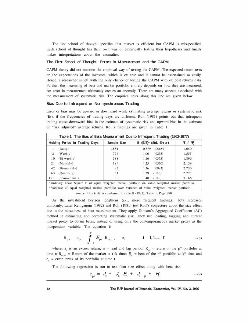
Bias Due to Infrequent or Non-synchronous Trading

Error or bias may be upward or downward while estimating average returns or systematic risk(�Es), if the frequencies of trading days are different. Roll (1981) points out that infrequenttrading cause downward bias in the estimate of systematic risk and upward bias in the estimateof “risk adjusted” average returns. Roll’s findings are given in Table 1.

As the investment horizon lengthens (i.e., more frequent tradings), beta increasesuniformly. Later Reinganum (1982) and Roll (1981) test Roll’s conjecture about the size effectdue to the biasedness of beta measurement. They apply Dimson’s Aggregated Coefficient (AC)method in estimating and correcting systematic risk. They use leading, lagging and currentmarket proxy to obtain betas, instead of using only the contemporaneous market proxy as theindependent variable. The equation is:

TteRaR itktmpk

T

nkptp ,...,2,1,, � ��

�� ¦ �E ...(8)

where, ap is an excess return; n = lead and lag period; R

pt = return of the pth portfolio at

time t; Rm,t+k

= Return of the market at t+k time; �Epk

= beta of the pth portfolio at kth time ande

it = error terms of its portfolio at time t.

The following regression is run to test firm size effect along with beta risk.

rp,t

= �J0, + �J1, �Ep, + �J2, p, + �Hp,...(9)

Table 1: The Bias of Beta Measurement Due to Infrequent Trading (1962-1977)

Holding Per iod in Trading Days Sample Size B (E/S)a (Std. Error ) �V2�H / �V2

sb

1 (Daily) 3881 0.879 (.00859) 1.050

2 (Weekly) 776 1.06 (.0235) 1.555

10 (Bi-weekly) 388 1.16 (.0375) 1.896

21 (Monthly) 184 1.25 (.0570) 2.159

42 (Bi-monthly) 92 1.36 (.0983) 2.730

63 (Quarterly) 61 1.39 (.116) 2.727

126 (Semi-annual) 30 1.48 (.186) 3.166a Ordinary Least Square �E of equal weighted market portfolio on value weighted market portfolio.b Variance of equal weighted market portfolio over variance of value weighted market portfolio.

Source: This table is condensed from Roll (1981), Table 1, Page 880.


where, rp,t

= Return in month t on market value portfolio p;

�Ep,y

= Estimated Dimson beta for portfolio p during year y;

Sp,y

= Logarithm of median firm size in portfolio p at the end of the year y-1;

and �0p,t

= Disturbance terms.

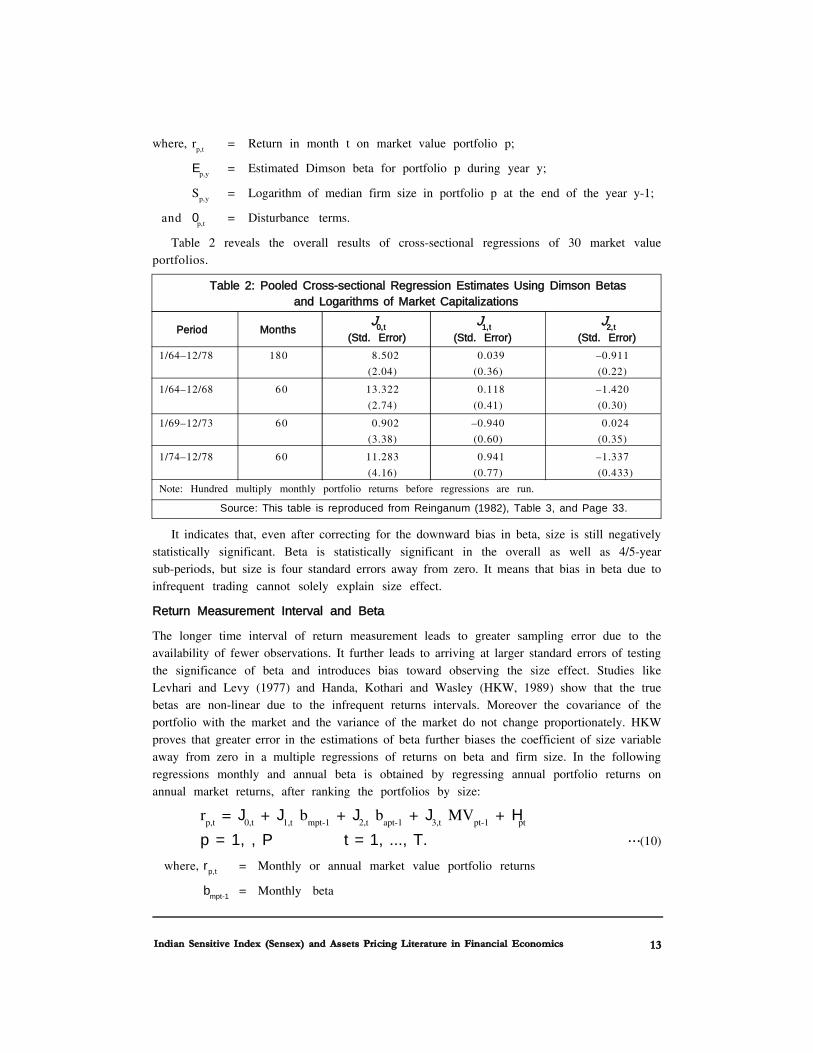
Table 2 reveals the overall results of cross-sectional regressions of 30 market valueportfolios.

Table 2: Pooled Cross-sectional Regression Estimates Using Dimson Betasand Logarithms of Market Capitalizations

Period Months�J

0,t�J

1,t�J

2,t

(Std. Error) (Std. Error) (Std. Error)

1/64–12/78 180 8.502 0.039 –0.911

(2.04) (0.36) (0.22)

1/64–12/68 60 13.322 0.118 –1.420

(2.74) (0.41) (0.30)

1/69–12/73 60 0.902 –0.940 0.024

(3.38) (0.60) (0.35)

1/74–12/78 60 11.283 0.941 –1.337

(4.16) (0.77) (0.433)

Note: Hundred multiply monthly portfolio returns before regressions are run.

Source: This table is reproduced from Reinganum (1982), Table 3, and Page 33.

It indicates that, even after correcting for the downward bias in beta, size is still negativelystatistically significant. Beta is statistically significant in the overall as well as 4/5-yearsub-periods, but size is four standard errors away from zero. It means that bias in beta due toinfrequent trading cannot solely explain size effect.

Return Measurement Interval and Beta

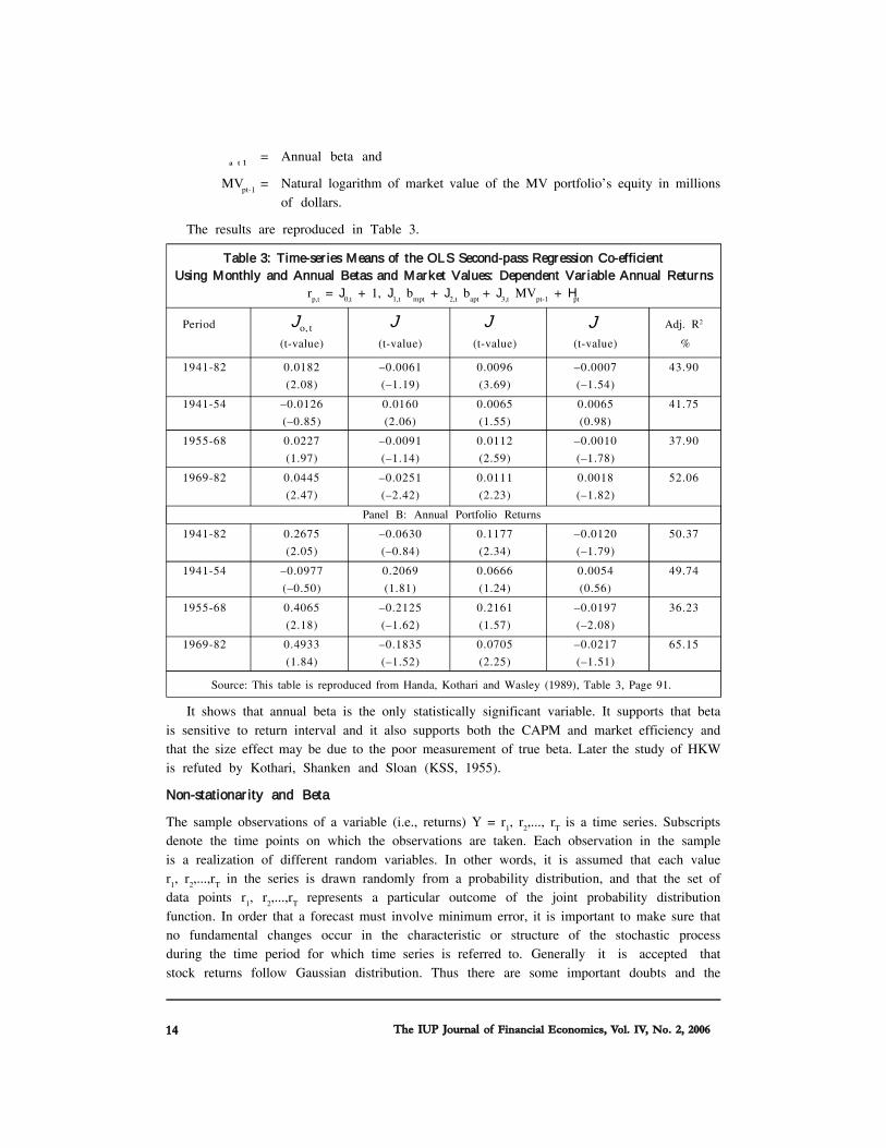
The longer time interval of return measurement leads to greater sampling error due to theavailability of fewer observations. It further leads to arriving at larger standard errors of testingthe significance of beta and introduces bias toward observing the size effect. Studies likeLevhari and Levy (1977) and Handa, Kothari and Wasley (HKW, 1989) show that the truebetas are non-linear due to the infrequent returns intervals. Moreover the covariance of theportfolio with the market and the variance of the market do not change proportionately. HKWproves that greater error in the estimations of beta further biases the coefficient of size variableaway from zero in a multiple regressions of returns on beta and firm size. In the followingregressions monthly and annual beta is obtained by regressing annual portfolio returns onannual market returns, after ranking the portfolios by size:

rp,t

= �J0,t

+ �J1,t

bmpt-1

+ �J2,t

bapt-1

+ �J3,t

MVpt-1

+ �Hpt

p = 1, …, P t = 1, ..., T. ...(10)

where, rp,t = Monthly or annual market value portfolio returns

bmpt-1 = Monthly beta


bapt-1

= Annual beta and

MVpt-1

= Natural logarithm of market value of the MV portfolio’s equity in millionsof dollars.

The results are reproduced in Table 3.

Table 3: Time-ser ies Means of the OLS Second-pass Regression Co-efficient Using Monthly and Annual Betas and Market Values: Dependent Var iable Annual Returns

rp,t

= �J0,t

+ 1, �J1,t

bmpt

+ �J2,t

bapt

+ �J3,t

MVpt-1

+ �Hpt

Period to,ˆ�J �J �J �J Adj. R2

(t-value) (t-value) (t-value) (t-value) %

1941-82 0.0182 –0.0061 0.0096 –0.0007 43.90

(2.08) (–1.19) (3.69) (–1.54)

1941-54 –0.0126 0.0160 0.0065 0.0065 41.75

(–0.85) (2.06) (1.55) (0.98)

1955-68 0.0227 –0.0091 0.0112 –0.0010 37.90

(1.97) (–1.14) (2.59) (–1.78)

1969-82 0.0445 –0.0251 0.0111 0.0018 52.06

(2.47) (–2.42) (2.23) (–1.82)

Panel B: Annual Portfolio Returns

1941-82 0.2675 –0.0630 0.1177 –0.0120 50.37

(2.05) (–0.84) (2.34) (–1.79)

1941-54 –0.0977 0.2069 0.0666 0.0054 49.74

(–0.50) (1.81) (1.24) (0.56)

1955-68 0.4065 –0.2125 0.2161 –0.0197 36.23

(2.18) (–1.62) (1.57) (–2.08)

1969-82 0.4933 –0.1835 0.0705 –0.0217 65.15

(1.84) (–1.52) (2.25) (–1.51)

Source: This table is reproduced from Handa, Kothari and Wasley (1989), Table 3, Page 91.

It shows that annual beta is the only statistically significant variable. It supports that betais sensitive to return interval and it also supports both the CAPM and market efficiency andthat the size effect may be due to the poor measurement of true beta. Later the study of HKWis refuted by Kothari, Shanken and Sloan (KSS, 1955).

Non-stationar ity and Beta

The sample observations of a variable (i.e., returns) Y = r1, r

2,..., r

T is a time series. Subscripts

denote the time points on which the observations are taken. Each observation in the sampleis a realization of different random variables. In other words, it is assumed that each valuer

1, r

2,...,r

T in the series is drawn randomly from a probability distribution, and that the set of

data points r1, r

2,...,r

T represents a particular outcome of the joint probability distribution

function. In order that a forecast must involve minimum error, it is important to make sure thatno fundamental changes occur in the characteristic or structure of the stochastic processduring the time period for which time series is referred to. Generally it is accepted thatstock returns follow Gaussian distribution. Thus there are some important doubts and the


crucial question is: Can the assumption of normally distributed returns be employed as aworking hypothesis? Most authorities would seem to accept that it could. (Allen, 1983).

However, the researchers of 1980s are worried about what happens to beta in case ofnon-stationarity of stock-returns because betas may affect size.

Some authors see these non-stationarity deviations as evidence of market inefficiency asthe prices deviate irrationally from the fundamental value. Others see that non-stationarity isattributed to the systematic changes in equilibrium in response of variation in beta risk. Theyargue that the failure to capture in beta risk may induce size and other effect.

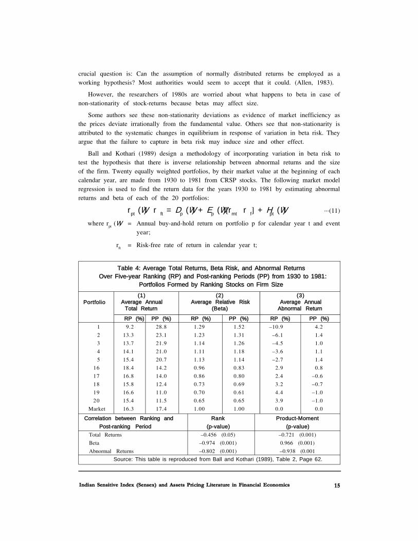
Ball and Kothari (1989) design a methodology of incorporating variation in beta risk totest the hypothesis that there is inverse relationship between abnormal returns and the sizeof the firm. Twenty equally weighted portfolios, by their market value at the beginning of eachcalendar year, are made from 1930 to 1981 from CRSP stocks. The following market modelregression is used to find the return data for the years 1930 to 1981 by estimating abnormalreturns and beta of each of the 20 portfolios:

rpt (�W) – rft = �Dp (�W) + �Ep (�W)[rmt – rf] + �Hpt (�W) ...(11)

where rpt (�W) = Annual buy-and-hold return on portfolio p for calendar year t and event

year;

rft

= Risk-free rate of return in calendar year t;

Table 4: Average Total Returns, Beta Risk, and Abnormal ReturnsOver Five-year Ranking (RP) and Post-ranking Periods (PP) from 1930 to 1981:

Portfolios Formed by Ranking Stocks on Firm Size

RP (%) PP (%) RP (%) PP (%) RP (%) PP (%)

1 9.2 28.8 1.29 1.52 –10.9 4.2

2 13.3 23.1 1.23 1.31 –6.1 1.4

3 13.7 21.9 1.14 1.26 –4.5 1.0

4 14.1 21.0 1.11 1.18 –3.6 1.1

5 15.4 20.7 1.13 1.14 –2.7 1.4

16 18.4 14.2 0.96 0.83 2.9 0.8

17 16.8 14.0 0.86 0.80 2.4 –0.6

18 15.8 12.4 0.73 0.69 3.2 –0.7

19 16.6 11.0 0.70 0.61 4.4 –1.0

20 15.4 11.5 0.65 0.65 3.9 –1.0

Market 16.3 17.4 1.00 1.00 0.0 0.0

Portfolio(1)

Average AnnualTotal Return

(2)Average Relative Risk

(Beta)

(3)Average Annual

Abnormal Return

Correlation between Ranking and Rank Product-Moment

Post-ranking Period (p-value) (p-value)

Total Returns –0.456 (0.05) –0.721 (0.001)

Beta –0.974 (0.001) 0.966 (0.001)

Abnormal Returns –0.802 (0.001) –0.938 (0.001

Source: This table is reproduced from Ball and Kothari (1989), Table 2, Page 62.


rmt

= Return on the market portfolio in calendar year t;

�Dp (�W) = Abnormal return in event year for portfolio p; and

�Ep (�W) = Systematic risk in event year for portfolio p.

The results are given in Table 4.

For small portfolios, post-ranking returns are largely higher than the ranking periodreturns. Variations in the betas seem to account for a substantial amount of abnormal returnsof firm size.

The Second School of Thought: Misspecification of Capital Market

In an efficient capital market, securities fully reflect available information instantaneously orvery quickly and provide unbiased estimates of the values of the underlying assets. When theintrinsic values are not reflected in prices, the predictability of stock returns is impaired.Logically, researchers conclude that market is inefficient both in the weak form and the semistrong form.

Brokerage, overreaction and misassessment of fundamentals are the main causes that makea capital market inefficient. The three sources of market inefficiency that may be consistentwith the size and book to market equity effects are described below.

Transaction Cost and Information Cost

The cost of broker’s commission, information-gathering cost, the cost of monitoring the firm’sactivities and the bid ask spread, in an imperfect market are the sources of market inefficiency.Black (1974) explains that transaction costs may hinder the market from quickly adjustingto earning announcements. Jones and Litzerberger (1970) argue that private costs ofprocessing and gathering earnings information are compensated by the excess returns. Priceadjustments due to the arrival of new information would be gradual (rather than instantaneous)because it takes time to disseminate the changes in fundamental values to the generalinvesting public. This allows the market professionals to make abnormal profit during thedecay of information transfer. This is only presumption. No professionals out beat the market.

Overreaction Hypothesis

Smidt (1968) notes that inappropriate responses to information costs by over-reaction ofinvestors about growth in earnings are other potential sources of market inefficiency. Basucalls this ‘over-reaction hypothesis’, ‘the price ratio hypothesis’.

DeBondt and Thalar (1985) provide a highly influential paper presenting the evidence ofsubstantial weak form of market inefficiency. They provide that there is negative correlationbetween systematic overreaction to new market information by the investors and the futureprice movements. The overreaction and future price movements are called price movementand price adjustment. The greater the initial price movement, the larger will be the subsequentprice adjustment. The empirical question is whether such stock price reversals are predictive.Analytically,

�> �@�� 0111 � � �� (u(r jtjtjt...(12)


where, 1��tf = The complete set of information at time t–1

rjt

= The return on security j at t

Em (rjt | m

tf 1�� ) = The expectation of rjt, assessed by the market on the basis of

the information set mtf 1��

Market efficiency implies (Em (u

wt| m

tf 1�� ) = (Em (u

1t| m

tf 1�� ) = 0, while overreaction

implies (Em (u

wt| m

tf 1�� ) < 0 and (Em (u

lt| m

tf 1�� ) > 0

DeBondt and Thaler’s findings are counter argued by Zerowin (1990), who finds that itis possible that overreaction hypothesis is largely driven by the January effect. Furthermore,the reversals of long-term returns documented by DeBondt and Thaler can also be explainedby Fama and French’s Three-Factor model (market, size and book-to-market equity ratio).

Systematic Misassessment in the Fundamentals

The third way of explaining anomalies in stock returns is simply blaming investors forirrational expectation and behavior. Dreman (1978) postulates that the mispricing of securitiesis due to bias in market expectations regarding earnings and earnings growth of low and highE/P firms. Earnings and growth of high E/P firms are systematically underestimated and thoseof the low E/P firms are systematically overestimated. Klein and Rosenfeld (1991) alsoattribute partially to security analyst’s consistent underestimation of reported earnings of firmswith the highest earnings yields.

The more important thing to find is that those who favor rational pricing theory have notyet derived a pricing model that can explain the empirical findings. Why are the abnormalreturns not arbitraged away by relatively more informed investors? Compared to naiveinvestors “experts” manage mutual funds and they must arrive at significant excess returnsbecause their strategies are superior. So far, most of the fund managers have not been able tobeat the market in the last several years.

These unanswered questions may make a person wonder if the evidence of the studyreviewed is just another example of statistical artefacts or perhaps there are missingfundamentals that researchers have yet to discover. This makes us lead to another approachof solving the puzzles by keeping the market efficient but the CAPM is misspecified.

Misspecification of the CAPM

These researchers say that CAP Model is misspecified. What is a good model? Harvey (1981)lists the following criteria or guidelines by which one can judge a model chosen in empiricalanalysis to be good/appropriate/right model:

• Parsimony: A model must be kept as simple as possible. The model can never completelycapture the reality; some amount of abstraction or simplification is inevitable;

• Identifiability: For a given set of data, there is only one estimate per parameter;

• Goodness of fit: The adjusted R2 (R– 2 ) is as high as possible;

• Theoretical consistency: In constructing a model, we should have some theoreticalunderpinning to it; measurement without theory often can lead to very disappointing


results. No matter how high the goodness of fit measures, a model may not be judged goodif one or more coefficients have a wrong signs; and

• Predictive power : One would choose a model whose theoretical predictions are borne outby actual experience.

Therefore, a model should be parsimonious in that it should include key variablesuggested by theory and relegate minor influences to the error term u. There are several waysin which a model can be deficient, called ‘specification errors’. The specification errors are:

• Omitting the relevant variable or under-fitting the model,

• Inclusion of irrelevant variables or over-fitting a model, and

• Incorrect functional form.

Fama and French (1995), consistent with rational pricing, report that the market portfolio,firm size and BEME factors in earnings explain the earnings of firms in the same way as thosecorresponding factors in returns explain stock returns. This suggests that market, size andBEME factors in earnings are the source of corresponding factors in returns. In CAPM thesevariables are not included. Hence, they argue, CAPM is misspecified. Ross (1976) proposesanother model which can accommodate any number of variables so as to explain fully thevariations in expected stock returns. The new model is called Arbitrage Pricing Theory.

Arbitrage Pr icing Theory and I ts Empir ical Tests

Ross (1976) develops the equilibrium returns of securities that are functions of a number offactors. Arbitrage Pricing Theory (APT) is more general and allows for the incorporation ofthe fundamental economic factors that can cause uncertainty in the market. The APT startswith the assumption that the stocks’ returns can be generated via the following factor model:

Ri = �D+ �E1i + �E2i + .. . + �Eni + �H ...(13)

where, n = Number of factors

�E1i

= The sensitivity of stock i to the first factor

�E2i

= The sensitivity of stock i to the second factor

�Eni

= The sensitivity of stock i to the nth factor

F1

= The magnitude of the first factor

F2

= The magnitude of the second factor.

Fn

= The magnitude of the nth factor

ri

= The rate of return of ith asset

ai

= The stocks expected return assuming the market is flat

ei

= A random amount that also does not depend on what happens in the rest ofthe market.

Basically, the APT is breaking down the market returns into its generation via fundamentaleconomic factors that are themselves uncertain and therefore are the root cause of the


uncertainty of stock’s return. A given stock’s non-diversifiable risk is thus a multi-factorconcept, given by the stocks sensitivities (or betas) with respect to individual economicfactors. Unfortunately, the APT, in itself, does not specify exactly what these factors are. It isup to economists and analysts to determine how many factors drive non-diversifiable marketrisk and what these factors are. The APT equation for determining a stocks required rate ofreturn as a function of risk is in general:

E(Ri) = r f + �Ei RP1 + �E2 RP2 + ... + �En RPn...(14)

where RPi = The risk premium associated with factor i.

This equation (14) is the multifactor APT counterpart to the CAPM equation. It makes noassumption about the probability distribution of risky assets, the market portfolio concept, themean variance efficient portfolio or the single period model constraint. It basically relies onthe-law-of-one-price to drive the model. That is, two securities with the same �Es are forcedto offer the same expected return. The central tenet of the model is that prices will adjust untilportfolios cannot be formed to achieve any arbitrage profit.

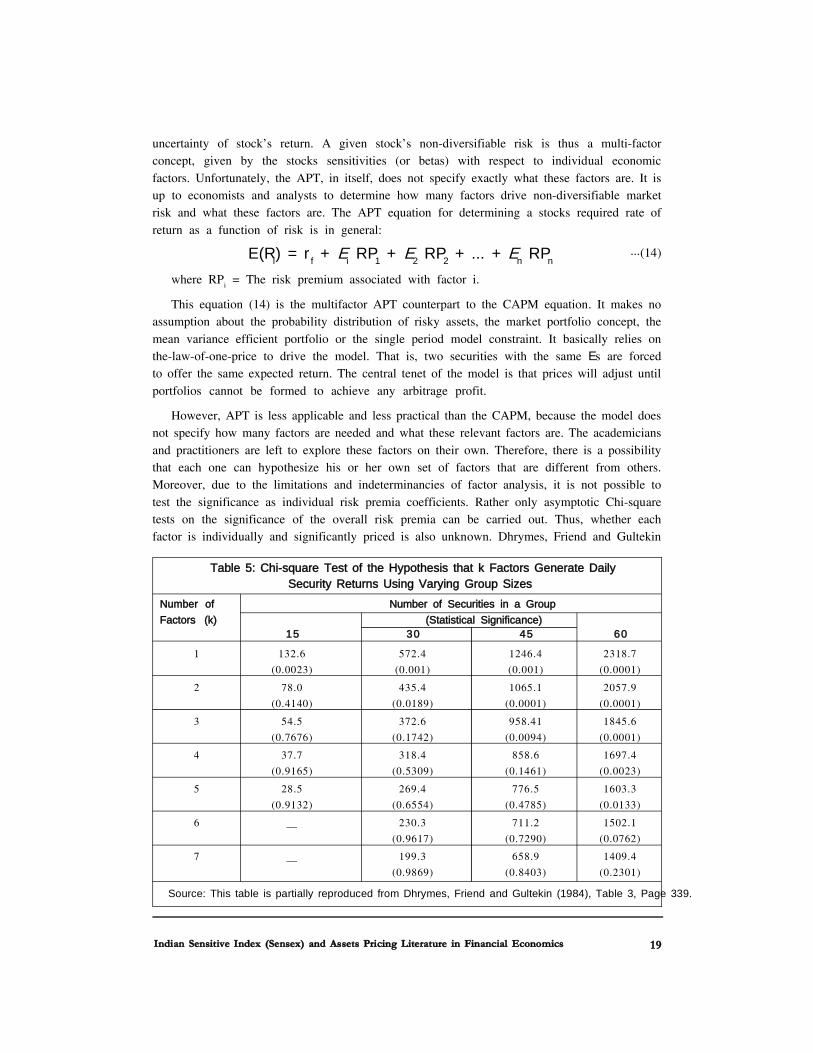
However, APT is less applicable and less practical than the CAPM, because the model doesnot specify how many factors are needed and what these relevant factors are. The academiciansand practitioners are left to explore these factors on their own. Therefore, there is a possibilitythat each one can hypothesize his or her own set of factors that are different from others.Moreover, due to the limitations and indeterminancies of factor analysis, it is not possible totest the significance as individual risk premia coefficients. Rather only asymptotic Chi-squaretests on the significance of the overall risk premia can be carried out. Thus, whether eachfactor is individually and significantly priced is also unknown. Dhrymes, Friend and Gultekin

Table 5: Chi-square Test of the Hypothesis that k Factors Generate DailySecurity Returns Using Varying Group Sizes

Number of Number of Securities in a Group

Factors (k) (Statistical Significance)15 30 45 60

1 132.6 572.4 1246.4 2318.7

(0.0023) (0.001) (0.001) (0.0001)

2 78.0 435.4 1065.1 2057.9

(0.4140) (0.0189) (0.0001) (0.0001)

3 54.5 372.6 958.41 1845.6

(0.7676) (0.1742) (0.0094) (0.0001)

4 37.7 318.4 858.6 1697.4

(0.9165) (0.5309) (0.1461) (0.0023)

5 28.5 269.4 776.5 1603.3

(0.9132) (0.6554) (0.4785) (0.0133)

6 — 230.3 711.2 1502.1

(0.9617) (0.7290) (0.0762)

7 — 199.3 658.9 1409.4

(0.9869) (0.8403) (0.2301)

Source: This table is partially reproduced from Dhrymes, Friend and Gultekin (1984), Table 3, Page 339.


(1984) and Dhrymes, Friend, Gultekin and Gultekin (1985) further report that the number offactors concluded by Ross are not robust to the number of securities in a group. Theydemonstrate that the number of factors found is proportional to the number of securities addedto a group. This proof is given in Table 5.

We can find that the significance level on each number of securities varies. At 5%significance level, for the 15 securities group, only one or two factors can be found. For 30securities group two or three can be found. The trend continues as securities in a groupincreases. The empirical research further questions how many factors are appropriate andsufficient for a multifactor model. The two-stage factor analysis for APT does not fare betterthan the CAPM against anomalies.

Macroeconomic Factors

The following are the major approaches to macroeconometric modeling:

• The traditional Cowles Commission structural equation approach,

• Unrestricted and Bayesian VaRs,

• Linear rational expectations models and

• The calibration approach associated with real business cycle theories.

In all these approaches, the main area of disagreement is over the relative roles ofeconomics and statistics: Should one aim to estimate a model derived from formal economictheory, or is it sufficient to find a model that accords well with the data.

Compared with natural sciences, where applied work has a profound influence in settingthe theoretical agenda by uncovering empirical puzzles that require a new theoretical toolsto deal with them, in economics, notwithstanding data problems, applied research does notreceive the attention that it deserves. The lack of widely accepted methodological frameworkfor applied economics is a major reason for this. The variation in stock return can beassociated with macroeconomic approach, where variations in risk premiums are due tomacroeconomic conditions. Chan, Roll and Ross (1986) argue that macroeconomic variableshould affect stock prices through changes in the discount rate and expected cash flow. Theyidentify four factors that might affect the discount rate:

1. The level of rates;

2. Term spread (spreads across different maturities);

3. Default spread (risk premium); and

4. Real consumption charges.

As for expected cash flow, changes in the expected level of real production should allinfluence current real value of cash flows. The following cross-sectional regression is run:

R = a + b mp

MP + bdei

DEI + bui UI + b

upr UPR + b

uts UTS + e ...(15)

where, R = Monthly returns on portfolios which are formed by size

MP = Monthly growth of industrial production


DEI = Change in expected inflation

UI = Unexpected inflation

UPR = Risk premium or term spread

UTS = Term structure or default spread

Flannery and Protopapadakis (2002) argue that stock market returns are significantcorrelated with inflation and money growth. The impact of real macroeconomic variables onaggregate equity returns is difficult to establish, perhaps because their effects are neither linearnor time invariant. They estimate a GARCH model of daily equity returns, where realizedreturns and their conditional volatility depend on 17 macro series’ announcements. They findsix candidates for priced factors: three nominal (CPI, PPI and a Monetary Aggregate) and threereal (Balance of Trade, Employment Report and Housing starts). Popular measures of overalleconomic activity, such as Industrial production or GNP are not represented.

In multifactor asset pricing models, any variable that effects the future investmentopportunity set or the level of consumption (given wealth) could be priced factor in equilibrium[Merton 1973), Breeden (1979)]. Macroeconomic variables are excellent candidates for the extramarket risk factors. However, the hypothesis that macroeconomic developments exertimportant effects on equity returns has strong intuitive appeal but little empirical support.

Microeconomic Factors

This kind of research with microeconomic factors may depend on the right explanatoryvariables, but the ex ante explanation is proven to be much more difficult. What is neededis a theoretical basis (similar to the CAPM) that can underlay what these fundamental factorsare in explaining stock returns. It’s just like sermon in a crowded church where the roombecomes stuffy. In this context, a window is drawn open to breath in fresh air, the CAPM isviewed from another angle which is of its own peculiar kind; in a class by itself: sui genericCAPM. The CAPM through behavioral finance (CAPM sui generis).

4. The Sui Generic CAPM

In his classic 1980 paper, Eugene Fama writes:

“[Efficient markets and asset pricing] research...did not begin with the development of atheory of price formation which was then subjected to empirical tests... Faced with theevidence, economists felt compelled to offer some rationalization... In short, there existeda large body by empirical results in search of a rigorous theory”

After nearly 40 years of exploration of the CAPM, DeBondt (2001) remarks:

“ Today, three decades later, the search for rigorous theory continues”.9

As before, stylized empirical facts constrain the various modeling effects. What is differentnowadays is that behavioral finance determines much of the empirical and theoretical agenda.

Behavioral finance is new. It studies how financial decisions in households, organizationsand markets are truly made. Decision processes are often crucial to decision outcomes. Thatis the main reason why behavioral finance borrows ideas from psychology. In contrast, modern


finance is based on the classical notation of ‘homo economics’, that is, the normative axiomsthat underlie expected utility theory, risk aversion, rational expectations etc. However, inexperiments, decision-makers systematically and often willingly violate the axioms ofrationality. In practice, when financial or other problem arises, there is often no unitary modelof truth, even through there are degrees of knowledge. The tacit models, that people are fluid,can be misleading and they are not internally consistent. Even when there is consistency, theinner logic is not Aristotelian logic of the type that says “one plus one is two”. Rather thelogic is psychological.10

Psychologists’ experiments show that human beings are not 100% rational decisionmakers. Shefrin and Statman (1984) use some of the psychologists’ results to argue thatinvestors may have an irrational preference for cash dividends.

Daniel, Hirshleifer and Subramanyam (1998) attempt to account for short-run momentumand long-run reversals in stock returns on two classical psychological biases in judgement:overconfidence and “biased self attribution”.

DeBondt (2001) finds in surveys, investors who tilt their portfolios toward equity are morelikely to see themselves as “leaders”, they “worry” less about the future, and they believe morefirmly that “entrepreneurial values benefit society”.

Nelson (2002) models rational herd behavior when the underlying value changes overtime, with payoffs that are either dependent or independent of the stock’s underlying value.He shows that herding does not last forever and is not monotone in single quality. Highcorrelation among agent’s actions does not necessarily imply herding.

Since the application of behavioral sciences including psychology to asset pricing is verylatest in financial economics, these may be well documented in future.

5. Empir ical Researches on the CAPM in India

Empirical research on the CAPM in India is few, as compared to the most developed countries’research on the CAPM. The main reason may be due to India’s percentage of equity marketcapitalization compared to world’s equity market capitalization is a meagre 0.69% (whereas,it is for USA 49.67%, Japan 13.04% and UK 9.67%).11 The other reasons are non-existenceof cohesiveness of research and publication and non-synchronization of doctoral researchbetween Indian universities. The total number of research publication on the CAPM comesbelow 50. These Indian research publications are subdivided into these categories:(1) Random Walk Hypothesis (RWH), (2) Indian Capital Market (ICM)’s Efficiency, (3) TheCapital Asset Pricing Model in Indian context and Offshoots of the CAPM inclusive of MarketMicrostructure and Anomalies. These are analyzed and discussed in the following.

Random Walk Hypothesis (RWH)

Krishna Rao (1971) tests RWH on Indian Aluminium weekly average share price data for aperiod of 16 years (1955-1970), collected from Calcutta Stock Exchange. Spectral analysisof the data indicates that RWH holds for Indian Aluminium. Sharma and Kennedy (1977) takethe last Friday share price data of each month for 132 observations each from India, UK andUSA for RWH. Spectral density confirms randomness of securities and the existence of RWHin ICM.


Indian Capital Market’s (ICM) Efficiency

Barua (1981) uses runs test and serial correlation test on 20 securities and on market index.He concludes that ICM is efficient. Sharma (1983) tests market efficiency with just 23 stocksduring the period 1973-1978 and concludes that ICM is fit for RWH only.

Krishna Rao’s (1988) sample is ten blue-chip companies for a period between 1982 and1987. He supports the hypothesis that ICM is weekly efficient. Maheswari and Vanjara (1989)take 142 securities for a period between 1980-1986 and conclude that market is not veryefficient. Pande and Ramesh Bhat (1989) collect and data from 600 users of accountinginformation about their perception about ICM, and he concludes in a nut shall that ICM isperceived to be inefficient. Obaidullah (1991) reports that risk-return parity does not exist inBombay Stock Exchange (BSE) and the market is efficient.

The Capital Asset Pricing Model (CAPM) in Indian Context

Gupta (1981) takes data, from Bombay, Calcutta and Madras Stock Exchanges, of 606 equityshares (from 1960-1976) with each year’s high and low prices of the stocks. He finds thatInvestment in equity shares is not a hedge against inflation and he doubts the applicabilityof the CAPM in ICM. Yalawar (1985) takes a sample of 122 actively traded scrips in BSE andshows that equity returns are high and consistent with market risk premium. He supports theCAPM that it is a good descriptor of ICM.

Varma (1988) studies capital asset pricing in India and he does not reject CAPM.Srinivasan (1988) takes quarterly annual data of 85 securities for a period of three years. Heconcludes that the CAPM does not exactly hold equilibrium theory in India. Obaidullah(1991a) finds the abnormal returns are observed to persist and concludes that the CAPMequilibrium is never reached in ICM. Obaidullah (1991b) tests the normality of stock returnsin India. He finds that daily returns are significantly different from normal distribution, yetthey are positively skewed and leptokurtic.

Sehgal (1993) takes the average prices of monthly low and high prices of 30 scrips ofSensex index over a period of ten years (1979-1989). The Sensex is also used a proxy for themarket. He concludes that the CAPM in India is a good indicator of asset pricing in all yearsexcept during recession. A die-hard CAPM fan.

Ray (1994) conducts a test of the CAPM using 170 actively traded scrip of BSE for aperiod of 11 years (1980-1991) and uses Fama-MacBeth methodology. He finds that theCAPM does not hold good for ICM. Obaidullah (1994) uses monthly stock price data of 30scrips for a period of 16 years (1976-1991). He finds that the results are contradictory. Thecoefficients of �E2 are generally not statistically significant, but �E2 are statistically significant inmultiple regressions. He concludes that the CAPM does not rest solidly in Indian stock market.

Gali (1995) tests for normality of returns of Sensex, The Economic Times index and Natexfrom 1987 till 1994 and concludes that the returns are normal for all the indices. Sehgal (1997)takes the three-moment model of the CAPM and his sample is 100 actively traded shares inBSE over a period of nine years (1984-1993) and finds that the average return on Indian stocksis 31.44% annualized (i.e., one can double the money in 2 ¼ years), yet his empirical findingsdo not support the CAPM in ICM.


Badhani (1997) attempts to analyze the effects of financial leverage on cost and valueof equity using the CAPM. His results do not confirm the consistency betweenModigliani-Miller hypothesis and the CAPM. Rao, Nath and Malhotra (1998) take 50 stocksof five year time interval and they conclude that their market proxy is an efficient portfolioand industry betas bear a linear relationship with mean quarterly returns, but it cannot betreated as a proof of validity of the CAPM in India.

Vipul (1998) tests CAPM’s return generation process in ICM compared to native rules. Hisdata is on 114 securities for seven years (1986-1993) in BSE. He finds that Market Modelholds good for ICM, two-factor CAPM does a better job of explaining return generationprocess and zero-beta return (R

z) is time variant in ICM.

Ansari (2000) takes 96 stocks from BSE over a period of seven years and finds that hisstudy casts a doubt on the validity of the CAPM as an asset-pricing model in India. However,he concludes that the game is not lost for the CAPM. Parchure and Uma (2000) formulateMarkowitz-model for solving portfolios that are efficient in a return-risk-liquidity sense intheir first part of the paper. These portfolios are more liquid and more diverse than standardMarkowitz portfolios. It is shown that the “potable” portfolios sometimes dominate theMarkowitz portfolios in terms of return and risk. The second part of the paper derives a generalversion of the CAPM, which is consistent with the empirical findings of an intercept greaterthan risk-free interest rate and a slope lesser than the market excess return.

Chaturvedi (2001) investigates parameter shift on earning announcements during1990-1998 and finds that the traditional market model parameters do not measure eventperiod abnormal returns accurately and he suggests using Bayesian procedure to reflect theshifts. Marisetty and Alayar (2002) test normality of Indian stock returns and find a significantpositive skewness and asymmetry in all the years between 1991 and 2001.

Offshoots of the CAPM Inclusive of Market Microstructure and Anomalies

In single-factor and two-factor model of the CAPM, �E is assumed to capture the average return

of stocks in the CAPM. In the 1980s and 1990s, various anomalous variables are takenatheoretically, resulting into the offshoots of the CAPM. In this section, we view the various

atheoretical effects tested in India.

Barua and Raghunathan (1986) study the efficiency of ICM and show that an investor

operating in the forward market can earn abnormal return, compared to an investor operating

in the cash market. Vasal (1988) studies on the effect of corporate financial decisions and share

price behavior in ICM and the results indicate that ICM is reasonably efficient in valuing a

firm.

Barua and Raghunathan (1990) calculate P/E ratio based on fundamental analysis of 23

stocks and compare them with actual P/E ratio. The results indicate that, on an average, shares

are overvalued in BSE. Agarwal (1991) looks into dividend and stock prices in commercial

vehicle sector in India for a period of 20 years (1966-1986). The adaptive expectation

hypothesis supports his findings that current net profit and two past dividends explain current

dividend behavior.


Vaidyanathan and Gali (1993) find that the average return on the first trading day isusually higher than that on the last trading day and intermediate days of settlement period.Madhusoodanan (1993) finds the extent of mean reversion of Indian stocks and concludes thatmost of the Indian stocks are mean reverting, though overall market shows a persistentbehavior. Madhusoodanan (1995) establishes that ICM also overreacts and hence thecontrarian strategy of selling past winners and buying past losers could produce excellentresults. Daterao and Madhusoodanan (1996) apply the theory of chaos and fractals to ICMand conclude that ICM shows chaotic behavior.

Poshakwale (1996) provides empirical evidence on weak-form efficiency andday-of-the-week effect in BSE over a period of seven years (1987-1994). He concludes thatBSE is efficient and day-of-the-weak effect persists in BSE. Mishra (1999) also finds thatreturns on Fridays are the highest.

Madhusoodanan (1997) attempts to find out the relationship between risk and expectedreturn and tests it to find if it is really positive or not, for 120 scrips in BSE for a period ofeight years (1987-1995). He finds that there is no positive relationship between beta and theexpected return. Karmakar (1997) tests hypothesis of volatility of share prices and explanationof volatility by fundamental economic factors. He concludes that noise-traders destabilize themarkets resulting “fads” or “bubbles”. Nageswara Rao (1997) examines the responses of stockprices to fiscal and monetary policy pronouncements, changes in industrial policy andchanges in exchange rate policy, amendments to Foreign Exchange Regulation Act (FERA)and regulatory action by Monopolies and Restrictive Trade Practices Commission (MRTPC).It is found that changes in administered prices seem to have the maximum impact on themarket.

Mohanty (1998) takes a smaller sample of 112 scrips and a larger sample of 2135 scripsto find out the impact of P/E effect, the book-to-market effect and size effect in ICM. He findsthat only book-to-market effect and P/E effect are more dominant and indexed stocks are notrepresentative of non-indexed stocks. Madhusoodanan (1998) applies the variance ratio testsunder the null hypothesis of homoscedasticity as well as heterocedasticity. He concludes thatRWH cannot be accepted in ICM and heterocedasticity does not play a major role in theIndian market. Sanyal and Sen (1998) attempts to examine how risk is diversified in India.Malhotra (1998) hypothesizes that the systematic risk of a company increases as the leverageis increased, and, a sample of ten companies from BSE for a period of four years (1993-1996)is taken. The closing prices of first four days of each month are observed, along with thatDebt/Equity ratio and returns of Sensex are taken. It is concluded that the hypothesis of apositive correlation between �E and debt-equity ratio is rejected.

Burman (1998) analyzes the stock prices data to find out if fundamentals or bubblesdetermine the changes in stock prices. He finds that the fundamentals are more important thanbubbles.

Mathew (1999) finds that the industry and firm level results support the informationcontent of dividend hypothesis. Chaturvedi (2000) analyzes the evidence of P/E effect inpre- and post-ranking announcement periods of 90 scrips in six years period (1990-1996).He concludes that significant P/E ratio effect exists in the market during the study period.


Shanmugham (2000) studies information sourcing by investors, their perception of variousinvestment strategy dimensions and the factors motivating share investment decisions. Hefinds that psychological and sociological factors dominate the economic factors in shareinvestment decisions. Anshuman and Goswami (2000) examines day-of-the-week effects onBSE, during the period 1991-1996 and finds evidence of heterocedasticity adjusted excesspositive returns of Fridays and excess negative returns on Tuesdays and the presence of badladoes not have any special influence on the day-of-the-week effect. Waghmare (2000) findsthat, though the ban on short sales does result in reducing ‘noise’ volatility, the same is nottrue in badla. There is also evidence of leverage effect in stock returns and its reversal duringthe period of ban. Karmakar and Chakraborthy’s (2000) results show that the averagepre-holiday returns are significantly higher than the mean returns of other days. Fridaysexhibit significantly positive returns.

Jha and Nagarajan (2002) examine market structure and efficiency of price transmittals inBSE and National stock Exchange using Johnson-Juselius multivariate cointegrationtechnique, and they find that some short run price movements stabilize and BSE and NSEappear to be reasonably efficient markets. They take 120 scrips for a period betweenJuly 1, 1996 and July 30, 1997.

6. Conclusion

The asset pricing founder Markowitz (1959) provides the genuine economic model within theframework of general equilibrium. Expectation of investors cannot be arrived at ex ante data(also called opportunity cost in the parlance of Economics) and the researcher has to dependon ex post data with strong reference to market index for the calculation of beta. Empiricalresearch after 1980s shows that �E alone is not the main price factor, other anomalous variablesare empirically tested by three school of thoughts in atheoretical models, but withcontradictory results. Going further on this track, asset pricing are under pinned onpsychological factors in sui generic CAPM. A brief review of Indian research on CAPM isgiven. All these researches are underpinned on market index. Since Indian barometer Sensexcrosses historical 10,000 marks, a passing remark of asset pricing literature with reference tomarket index is discussed.�Y

Reference # 42J-2006-06-01-01


End Notes1 An excellent article is given on the “The Three P’s of Total Risk Management” by Andrew

W Lo (1999), Financial Analysts Journal, January-February 1999, pp. 13-26.

2 The fundamental axioms are on the basis of five assumptions: (1) Transitivity,(2) Continuity of preference, (3) Independence, (4) High probability of success and(5) Compound probabilities. See Finance—A Theoretical Introduction by David E Allen,(1983), Martin Robertson, Oxford, pp. 60-2.

3 Andrew Lo, op.cit.,

4 John Y Campbell, (2000), “Asset Pricing at the Millennium”, The Journal of Finance,Vol. LV. No. 4, pp. 1516-67.

5 Bollerlev, Tin and Robert J Jodrick (1999). “Financial Market Efficiency Tests”,Handbook of Applied Economics, Vol. I Macroeconomics, eds. M Hashem Pesaran andMichael R Wickens, Blackwell Publishers, 1999, UK.

6 Fair Game Model says that, on average, across a large number of observations, theexpected return on an asset, given information set, Info, will equal its actual return. Theappropriate mathematical expression is:

tj

tjttj

tj

tjtjtj P

PInfoPE

P

PP

,

,1,

,

,1,1,

)( ��

��

��H ...(1)

where, Pj,t+1

= The actual price of security j next period

Pj,t

= The price of security j this period

E(Pj,t+1)

| Infot) = The predicted (or expected) security price next period, given a

current amount of information, infot

�Hj, t+1

= The difference between actual and predicted returns.

Fair Game Model (1) is really written in returns form. Let one period return be defined as

tj

tjtjiij P

PPr

,

,1,1,

��

��...(2)

then (1) can be written as

�Hj, t+1

= r j,t+1

- E(rj, t+1

| Infot) ...(3)

If we take the expectation of (3), the price pattern will be a fair game if the expecteddifference between the actual and the predicted return is equal to zero.

E(�Hj, t+1

) = E (r j, t+1

– E (rj, t+1

| Infot )) = 0

Let the value of a portfolio be xt i.e., x

t = h

t P

t where h

t = number of shares at the beginning

of the period t and Pt = price at t. The expected future value of x

t is E

t(x

t+1) and it is equal

to (1+r) ht P

t or (1+r) x

t, x

t is a martingale (r=0). If r > 0, x

t is a submartingale or if r < 0,

xt is a supermartingale.


7 John Y Campbell (2000), op cit.,

8 Courtesy:

• Lin, Chien-Jung and R Stephen Sears Misspecification of CAPM: Implication forSize and Book-to-Market Effect, February 2001; on-line, Internet, January 14, 2002,Available FTP: bs. ac. cowan.edu/au/fbe/wps/working paper / pdffiles/wp0102el.pdf.

• Brealey, Richard A, and Stewart C Myres. Principles of Corporate Finance , Tata,McGraw-Hill, 1997, pp. 224-30.

• Chien-Ting Lin, “Misspecification of Capital Asset Pricing Model (CAPM):Implication for Size and Book-to-market Effects”, Unpublished Doctoral Dissertation,Texas Tech University, May, 1999.

9 DeBondt, W.F.M., (2001), “Cultural Factors in Investment Decision Making”, WorkingPaper, University of Wisconsin-Madison.

10 See 8 above.

11 Comparative size of World Equity Markets in USD (for Morgan Stanley CapitalInternational: Methodology and Index Policy, 1998), quoted by Andor, György, MihályOrmos and Balázs Szabó, “Empirical Tests of Capital Asset Pricing Model (CAPM) in theHungarian Capital Market”, Periodica Polytechnica Ser.Soc.Man.Sci., Vol. 7, p. 62.

References

1. Agarwal R N (1991), “Dividends and Stock Prices: A Case Study of Commercial VehicleSector in India 1966-67 to 1986-87”, Indian Journal of Finance and Research, Vol. 1,pp. 61-7.

2. Allen, David E (1983), Finance-A Theoretical Introduction, Mertin Robertson, Oxford.

3. Ansari, Valeed A (2000), “Capital Asset Pricing Model: Should We Shop Using it?”Vikalpa, Vol. 25, No. 1, pp. 55-64.

4. Anshuman, Ravi V, and Ranadev Goswami, (2000), “Day-of-the-Week Effects on the Bombay Stock Exchange”, The IUP Journal of Applied Finance, Vol. 6, No. 4, pp. 31-46.

5. Bachelier, Louis (1900), “Théorie de la Spéculation”, Annales Scientifiques de l’EcoleNormale Supérieure 17 (3rd Series 1900), pp. 21-88; Translated from French into Englishby A J Boness, “The Theory of Speculation” in The Random Character of Stock MarketPrices, edited by P H Cootner (Risk Publications 2000), pp. 18-91.

6. Badhani, K N (1997), “Effects of Financial Leverage on Systematic Risk, Cost and Valueof Equity under Capital Asset Pricing Model”, Finance India , Vol. XI, No. 2, pp. 343-352.

7. Ball R and S P Kothari (1989), “Nonstationary Expected Returns: Implications for Testsof Market Efficiency and Serial Correlation in Returns,” Journal of FinancialEconomics, Vol. 25, pp. 51-74.


8. Barua S K (1981), “The Short-run Price Behavior of Securities: Some Evidence onEfficiency of Indian Capital Market”, Vikalpa, Vol. 6, pp. 93-100.

9. Barua S K and Raghunathan V (1986), “Inefficiency of the Indian Capital Market”,Vikalpa, July-September, Vol. 11, No. 3, pp. 225-229.

10. Barua S K and Raghunathan V (1990), “Soaring Stock Prices: Defying Fundamentals”.Economic and Political Weekly, November 17, Vol. 25, No. 46, pp. 2559-61.

11. Bernoulli, Daniel (1738), “Specimen Theoriae Novae de Mensura Sortis” in CommentariiAcademiae Scientiarium Imperialis Petropolitannae ; translated from Latin into Englishby L Sommer, “Exposition of a New Theory on the Measurement of Risk”, Econometrica22, No. 1, (January 1954), pp. 23-36.

12. Black F (1974), “Can Portfolio Managers Outrun the Random Walkers?” Journal ofPortfolio Management, Vol. 1, pp. 32-36.

13. Breeden D (1979), “An Intertemporal Capital Pricing Model with Stochastic InvestmentOpportunities”, Journal of Financial Economics , Vol. 7, No. 3, pp. 265-96.

14. Breeden D (1979), “An Intertemporal Capital Pricing Model with Stochastic InvestmentOpportunities”, Journal of Financial Economics , Vol. 7, No. 3, pp. 265-96.

15. Burman R B (1998), “What Determine the Prices of Indian Stocks: Fundamentals orBubbles? The IUP Journal of Applied Finance, pp. 245-254.

16. Campbell J, Lo A and MacKinlay A C (1997), The Econometrics of Financial Markets,Princeton University Press.

17. Chan, Roll N R and Ross S (1986) “Economics Forces and the Stock Market,” Journalof Business, Vol. 56, pp. 83-403.

18. Chaturvedi, Hari Om (2000), “Anomalies Based on P/E Ratios: Empirical Evidence from the Indian Stock Market,” IUP Journal of Applied Finance, Vol. 6, No. 3, pp. 1-13.

19. Chaturvedi, Hari Om (2001), “Parameter Shift in Event Studies: The Case of EarningsAnnouncements,” Prajnan , Vol. XXIX, No. 1, pp. 303-314.

20. Cox J, Ingersoll J and Ross S (1985), “An Intertemporal General Equilibrium Model ofAsset Prices”, Econometrica, Vol. 53, No. 2, pp. 363-84.

21. Daniel K, Hirshleifer D and Subramanyam A (1998), “Investor Psychology and SecurityMarket under and Observations,” Journal of Finance , 53, pp. 1839-86.

22. Daterao M and T P Madhusoodanan, (1996), “Fractals and Chaos: Application to theIndian Stock Market”, Working paper No. 7, UTI Institute of Capital Markets.

23. De Finetti B (1937), La Prevision: Ses Lois Loguiques, Ses Sources Subjectives.Translated into English by H Kyburg and H Smoklerm eds. 1964. Studies in SubjectiveProbability , New York: John Wiley & Sons.


24. De Finetti B (1937), “La Prévision: Ses Lois Logiques, Ses Sources Subjectives”. Annalesde l’Institut Henri Poincaré, Vol. 7, pp. 1-68. Translated into English in H Kyburg andH Smokler, eds. 1964. Studies in Subjective Probabilitiy. New York: John Wiley & Sons.

25. DeBondt W F M (2001), “Cultural Factors in Investment Decision Making”, WorkingPaper, University of Wisconsin-Madison.

26. DeBondt W F M and R Thaler (1985), “Does the Stock Market Overreact?” Journal ofFinance , Vol. 40, pp. 557-581.

27. Debreu, Gerard (1959), Theory of Value, The Cowles Foundation Monograph 17, 1959.

28. Dhrymes P, I Friend, and N B Gultekin (1984), “A Critical Reexamination of theEmpirical Evidence on the Arbitrage Pricing Theory,” Journal of Finance , Vol. 39,pp. 323-346.

29. Dhrymes P, I Friend, M N Gultekin, and N B Gultekin (1985), “New Tests of the APTand Their Implications,” Journal of Finance , Vol. 40, pp. 659-674.

30. Dimson, E (1979), “Risk Measurement when Shares are Subject to Infrequent Trading,”Journal of Financial Economics , Vol. 7, pp. 197-226.

31. Fama, E F (1976), Foundations of Finance , New York: Basic Books.

32. Fama E F (1980), “Efficient Capital Markets: A Review of Theory and Empirical Work”,Journal of Finance, XXV, pp. 383-417.

33. Fama E F, and K R French (1995), “Size and Book-to-market Factors in Earnings andReturns”, Journal of Finance, Vol. 50, pp. 131-55.

34. Flannery, Mark J, and A Protopapadakis Aris (2002), “Macroeconomic Factors DoInfluence Aggregate Stock Returns”, The Review of Financial Studies, Summer, Vol. 15,No. 3, pp. 751-82.

35. Handa, Puneet, S P Kothari and Charles Wasley (1989), “The Relation Between ReturnInterval and Betas: Implication for the Size Effect”, Journal of Financial Economics, 23,pp. 79-100.

36. Jones C P, and R H Litzenberger (1970), “Quarterly Earnings Reports and IntermediateStock Price Trends,” Journal of Finance , Vol. 25, pp. 14-148.

37. Karmakar M (1997), “Share Price Volatility and Efficient Market Hypothesis—AnAnalysis of Indian Experiences,” Finance India , Vol. XI, No. 3, pp. 685-688.

38. Karmakar M and M Chakraborty (2000), “Holiday Effect in the Indian Stock Market,”Finance India , Vol. XIV, No. 1, pp. 165-172.

39. Karmakar, M and M Chakraborty (2000), “Holiday Effect in the Indian Stock Market,”Finance India , Vol. XIV, No. 1, pp. 165-172.


40. Klein A and J Rosenfeld (1991), “PE Ratios, Earnings, Expectations, and AbnormalReturns”, Journal of Financial Research , Vol. 14, pp. 51-64.

41. Kothari S P, J Shanken and R Sloan (1995), “Another Look at the Cross-section ofExpected Stock Returns”, Journal of Finance , Vol. 50, pp. 185-224.

42. Levhari D and H Levy (1977), “The Capital Asset Pricing Model and the InvestmentHorizon,” Review of Economics and Statistics, Vol. 59, pp. 92-104.

43. Lucas R (1978), “Asset Prices in an Exchange Economy”, Econometrica, Vol. 46, No. 6,pp. 1429-46.

44. Madhusoodanan T P (1995), “Optimal Portfolio Selection: A Performance Analysis withIndian Stock Market Returns”, Working Paper No. 2, UTI Institute of Capital Markets.

45. Madhusoodanan T P (1997), “Risk and Return: A New Look at the Indian Stock Market”,Finance India , Vol. XI, No. 2, pp. 285-304.

46. Madhusoodanan T P (1998), “Persistence in the Indian Stock Market Returns: AnApplication of Variance Ratio Test”, Vikalpa, Vol. 23, No. 4, pp. 61-73.

47. Maheswari G C and K R Vanjara (1989), Risk Return Relationship: A Survey of SelectedEquity Shares, in Stock Market Efficiency and the Price Behavior (The Indian Experience),ed. by O P Gupta, First Edition, Anmol Publication, New Delhi, pp. 335-52.

48. Malhotra, Minakshi (1998), “Capital Structure and Systematic Risk—An Interrelationshipin Indian Industries”, Journal of Accounting and Finance , Vol. 12, No. 1, pp. 87-94.

49. Malhotra, Minakshi (1998), “Capital Structure and Systematic Risk—An Interrelationshipin Indian Industries”, Journal of Accounting and Finance , Vol. 12, No. 1, pp. 87-94.

50. Marisetty, Vijaya B and Vedpuriswar Alayar (2002), “Asymmetry in Indian Stock Returns—An Empirical Investigation,” The IUP Journal of Applied Finance, Vol. 8, No. 2, pp. 14-20.

51. Markowitz H M (1952), “Portfolio Selection and Foundation of Portfolio Theory”,Journal of Finance , pp. 469-477.

52. Mathew P A (1999), “Indian Stock Markets: Empirical Evidence on the InformationContent of Dividend Hypothesis”, Journal of Accounting and Finance , Vol. 13, No. 2,pp. 51-65.

53. Merton R (1973), “An Intertemporal Capital Asset Pricing Model”, Econometrica,Vol. 41, No. 5, pp. 867-87.

54. Mishra, Bishnupriya (1999), “Presense of Friday Effect in the Indian Stock Market”,Paradigm , Vol. 3, No. 2, pp. 57-64.

55. Mohanty Pitabas (1998), “On the Cross Section of Stock Returns: The Effect of Sample Size on the Research Findings”, The IUP Journal of Applied Finance, pp. 306-18.


56. Nageswara Rao S V D (1997), “Response of Stock Prices to Macroeconomic Events”,Finance India , Vol. XI, No. 4, pp. 881-918.

57. Nelson Lee (2002), “Persistence and Reversal in Herd Behavior: Theory and Applicationto the Decision to Go Public”, The Review of Financial Studies, Spring, pp. 65-95.

58. Obaidullah M (1991a), “Earnings, Stock Prices and Market Efficiency: Indian Evidence, Se-curities Industry Review”, Journal of the Singapore Securities Research Institute , October.

59. Obaidullah M (1991b), “The Price-Earnings Ratio-anomaly in Indian Stock Markets”,Decision, July-September.

60. Obaidullah M (1991), “The Distribution of Stock Returns”, Charted Financial Analyst,pp. 17-31.

61. Pandey I M and Ramesh Bhat, (1989), Efficient Market Hypothesis: Understanding andAcceptance in India, in Stock Market Efficiency and the Price Behavior (the IndianExperience), Edited by O P Gupta, First Edition, Anmol Publication, New Delhi, pp. 279-93.

62. Parchure Rajas and S Uma (2000), Potable Portfolios, Indian Capital Markets—Trendsand Dimensions, Eds. Uma Shashikant and S Arumugam, Tata MacGraw-Hill PublishingCompany Ltd., Delhi.

63. Poshakwale Sunil (1996), “Evidence on Weak form Efficiency and Day of the WeekEffect in the Indian Stock Market”, Finance India , Vol. X, No. 3, pp. 605-616.

64. Ramsey F (1926), “Truth and Probability”, Foundations of Mathematics and OtherLogical Essays, R Braithwaite (Ed), New York: Harcourt Brace.

65. Ramsey F (1926), Foundations of Mathematics and Other Logical Essays.R Braithwaite (Ed). New York: Harcourt Brace.

66. Rao C V, Golaka C Nath and Manish Malhotra (1998), “Capital Asset Pricing Model andIndian Stocks”. The IUP Journal of Applied Finance, reprinted in Research Papers in Applied Finance .

67. Rao N Krishna (1988), “Stock Market Efficiency: The Indian Experience”, PaperPresented at ‘National Seminar or Indian Securities Markets: Thrusts and Challengers’,Organized by the Department of Commerce, University of Delhi, South Campus,March 24-26, 1988. Reproduced in Stock Market Efficiency and the Price Behavior(The Indian Experience), Edited by O P Gupta, First Edition, 1989, Anmol Publication,New Delhi, pp. 203-18.

68. Rao, N Krishna and K Mukherjee (1971), “Random Walk Hypothesis: An EmpiricalStudy”, Arthaniti, Vol. 14, Nos. 1 and 2, pp. 53-58, Reproduced in Stock MarketEfficiency and the Price Behavior (the Indian Experience), Edited by O P Gupta, FirstEdition, 1989, Anmol Publication, New Delhi, pp. 99-105.


69. Ray, Subrata, “Capital Asset Pricing Model—The Indian Context”, Unpublished DoctoralDissertation, Indian Institute of Management, Bangalore, 1994.

70. Reinganum, M R (1982), “A Direct Test of Roll’s Conjecture on the Firm Size Effect,”Journal of Finance, Vol. 37, pp. 27-35.

71. Roll R (1981), “A Possible Explanation of the Small Firm Effect, “Journal of Finance,pp. 879-888.

72. Ross S A (1976), “The Arbitrage Theory of Capital Asset Pricing”, Journal of EconomicTheory, Vol. 13, pp. 3341-60.

73. Sanyal G and S Sen (1998), “Portfolio Diversification and Risk Redmetion in India—An Empirical Analysis”, Finance India, Vol. XII, No. 2, pp. 375-383.

74. Savage L (1954), Foundations of Statistics, New York: John Wiley & Sons.

75. Savage L (1954), Foundations of Statistics, New York: John Wiley & Sons.

76. Sehgal Sanjay (1993), “The Distribution of Stock Market Returns: Tests of Normality”,Indian Journal of Finance and Research, Vol. V, No. 2, July.

77. Sehgal Sanjay (1997), “An Empirical Testing of Three-Parameter Capital Asset PricingModel in India”, Finance India, Vol. XI, No. 4, pp. 919-40.

78. Shanmugam, R (2000), Factors Influencing Investment Decisions in Indian CapitalMarket—Trends and Dimensions, Tata MacGraw-Hill Company Ltd. New Delhi.

79. Sharma J L (1983), “Efficient Capital Markets and Random Character of Stock PriceBehavior in a Developing Economy”, Indian Economic Journal, October-December,Vol. 31, No. 2, pp. 53-70, Reproduced in Stock Market Efficiency and the PriceBehaviour (The Indian Experience), Edited by O P Gupta, First Edition, 1989, AnmolPublication, New Delhi, pp. 219-43.

80. Sharma J L and Robert E Kennedy (1977), “Comparative Analysis of Stock PriceBehavior on the Bombay, London, and New York Stock Exchanges”, Journal ofFinancial and Quantitative Analysis, September, Vol. 12, No. 3, pp. 391-413.

81. Sharpe W F (1963), “A Simplified Model for Portfolio Analysis”, Management Science,January, pp. 277-293.

82. Shefrin H and M Statman (1984), “Explaining Investor Preference for Cash Dividends”,Journal of Financial Economics, 13, pp. 253-82.

83. Smidt S (1968), “A New Look at the Random Walk Hypothesis”, Journal of Financialand Quantitative Analysis, pp. 235-262.

84. Srinivasan N P and M S Narasimhan (1988), “Testing Stock Market Efficiency UsingRisk-Return Parity Rule”, Vikalpa, April-June, Vol. 13, No. 2, pp. 61-66.


85. Vaidyanathan R and Kanti Kumar Gali (1993), “Stock Market Returns and “Vallan”(Settlement Period) Effect”, Chartered Financial Analyst , December, Vol. 8, No. 12,pp. 5-10.

86. Varma Jayant Rama (1988), Asset Pricing under Parameter Non-stationarity , FPMThesis, Indian Institute of Management, Ahmedabad.

87. Vasal V K (1988), “Corporate Financial Decisions and Share Price Behavior in India”,Paper presented at ‘National Seminar on Indian Securities Markets: Thrusts andChallenges’, organized by the Department of Commerce, University of Delhi, SouthCampus, March 24-26, 1988. Reproduced in Stock Market Efficiency and the PriceBehaviour (The Indian Experience), Edited by O P Gupta, First Edition, AnmolPublication, New Delhi, pp. 245-53.

88. Vipul (1998), “CAPM: Does it Help in Indian Capital Market?,” Finance India , Vol. XII,No. 1, pp. 1-19.

89. von Neumann J and O Morganstern, (1944), Theories of Games and Economic Behvior,Princeton University Press.

90. Waghmare, Tushar (2000), “Volitility in India Stock Markets: A Study of Badla and ShortSales Restrictions” in Indian Capital Market—Trends and Dimensions, Tata MacGraw-HillCompany Ltd. New Delhi.

91. Williams, John Burr (1938), The Theory of Investment Value, North-Holland, Amsterdam,1964.

92. Yalawar Y B (1985), “Bombay Stock Exchange: Rates of Return and Efficiency”, Paperpublished by Indian Institute of Management, Bangalore.

93. Zarowin P (1990), “Size, Seasonality, and Stock Market Overreaction,” Journal ofFinancial and Quantitative Analysis , Vol. 25, pp. 113-125.

Documents

Indian Sensitive Index (Sensex) and Assets Pricing ...Indian Sensitive Index (Sensex) and Assets Pricing Literature in Financial Economics 7 The rest of the paper is organized as follows: