2003 IEEE/RSJ International Conference on Intelligent Robotsand Systems (IROS), Vol. 2, October, 2003, pp. 1808-1813.

Inertial Navigation and Visual Line Following fora Dynamical Hexapod RobotSarjoun Skaff, George Kantor, David Maiwand, Alfred A. Rizzi

sarjoun, kantor, dm597, arizzi@ri.cmu.eduThe Robotics Insititute, Carnegie Mellon University, Pittsburgh, PA

Abstract— This paper presents preliminary development ofautonomous sensor-guided behaviors for a six-legged dynamicalrobot (RHex). These behaviors represent the first exteroceptiveclosed-loop locomotion strategies for this system. Simple motionmodels for RHex are described and used to deploy controllersfor inertial straight line locomotion and visual line following.Results are experimentally validated on the robot.

I. I NTRODUCTION

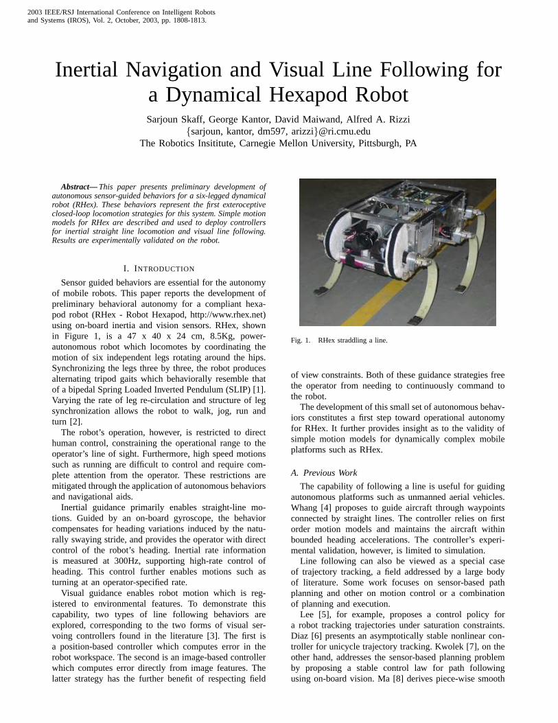
Sensor guided behaviors are essential for the autonomyof mobile robots. This paper reports the development ofpreliminary behavioral autonomy for a compliant hexa-pod robot (RHex - Robot Hexapod, http://www.rhex.net)using on-board inertia and vision sensors. RHex, shownin Figure 1, is a 47 x 40 x 24 cm, 8.5Kg, power-autonomous robot which locomotes by coordinating themotion of six independent legs rotating around the hips.Synchronizing the legs three by three, the robot producesalternating tripod gaits which behaviorally resemble thatof a bipedal Spring Loaded Inverted Pendulum (SLIP) [1].Varying the rate of leg re-circulation and structure of legsynchronization allows the robot to walk, jog, run andturn [2].

The robot’s operation, however, is restricted to directhuman control, constraining the operational range to theoperator’s line of sight. Furthermore, high speed motionssuch as running are difficult to control and require com-plete attention from the operator. These restrictions aremitigated through the application of autonomous behaviorsand navigational aids.

Inertial guidance primarily enables straight-line mo-tions. Guided by an on-board gyroscope, the behaviorcompensates for heading variations induced by the natu-rally swaying stride, and provides the operator with directcontrol of the robot’s heading. Inertial rate informationis measured at 300Hz, supporting high-rate control ofheading. This control further enables motions such asturning at an operator-specified rate.

Visual guidance enables robot motion which is reg-istered to environmental features. To demonstrate thiscapability, two types of line following behaviors areexplored, corresponding to the two forms of visual ser-voing controllers found in the literature [3]. The first isa position-based controller which computes error in therobot workspace. The second is an image-based controllerwhich computes error directly from image features. Thelatter strategy has the further benefit of respecting field

Fig. 1. RHex straddling a line.

of view constraints. Both of these guidance strategies freethe operator from needing to continuously command tothe robot.

The development of this small set of autonomous behav-iors constitutes a first step toward operational autonomyfor RHex. It further provides insight as to the validity ofsimple motion models for dynamically complex mobileplatforms such as RHex.

A. Previous Work

The capability of following a line is useful for guidingautonomous platforms such as unmanned aerial vehicles.Whang [4] proposes to guide aircraft through waypointsconnected by straight lines. The controller relies on firstorder motion models and maintains the aircraft withinbounded heading accelerations. The controller’s experi-mental validation, however, is limited to simulation.

Line following can also be viewed as a special caseof trajectory tracking, a field addressed by a large bodyof literature. Some work focuses on sensor-based pathplanning and other on motion control or a combinationof planning and execution.

Lee [5], for example, proposes a control policy fora robot tracking trajectories under saturation constraints.Diaz [6] presents an asymptotically stable nonlinear con-troller for unicycle trajectory tracking. Kwolek [7], on theother hand, addresses the sensor-based planning problemby proposing a stable control law for path followingusing on-board vision. Ma [8] derives piece-wise smooth

controllers for trajectory tracking directly in image space.The work presented here also centers on sensor-basednavigation, but adopts simple control policies to evaluatetheir efficacy on robots with complex dynamics.

Similarily to the work of Murrieri [9], the approachtaken here on FOV constrained navigation is inspired byLyapunov theory, but offers the additional advantage ofavoiding nonsmooth switching.

II. A PPROACH

Three approaches for sensor-guided behavior are de-scribed here. The first is a controller that uses inertialsensing to steer the robot and the remaining two arevision–based line following controllers.

A. Motion Models for RHex (Templates)

The SLIP and Lateral Leg Spring (LLS) [10] templatesdescribe RHex’s motion in the sagital and horizontalplanes, respectively. These models have limited applica-tion for robot control, however, because their anchoringin the physical system is yet unavailable.

A simpler horizontal motion model is the kinematicunicycle. Similarly to unicycles, RHex is subject to non-holonomic constraints preventing lateral motion and iscontrolled through forward and rotational velocities. Sys-tem identification of the steering behavior indicates thataccurate unicycle models grow in comlexity as the robotgains speed [11]. In the standard unicycle coordinates en-coding position and orientation (Figure 2), the kinematicsare written as

d

dt

x

y

θ

=

vfcosθvf sinθ

0

+

00u

. (1)

Here the control inputs areu and vf , specifying theangular and forward velocities of the robot, respectively.

H

D 1

projection of

image plane

line to follow

(x-axis)

y

x

(x,y)

qrobot

w1

Hw2

Fig. 2. Simplified model of robot and camera configurations, top view.

B. Inertia-guided Navigation

The purpose of inertial guidance is to control the robot’sheading at all speeds. Experiments show that adjustingthe gait offset directly controls the angular velocity [2],affecting only the third row of (1). To accomplish headingcontrol, u is set proportional to the heading error,

u = κp

(

θ − θ)

, (2)

with θ and θ representing the current and desiredheading of the robot, respectively.

As predicted by [11], the complexity of the steeringdynamics increases at running speed. Empirical evidencesuggests that the heading dynamics are better modeled asa second order system of the form

θ = −dθ + u, (3)

with d > 0. Accordingly, at running speed, the policy

u = κp

(

θ − θ)

+ κd

(

θ − ˙θ)

(4)

stabilizes the heading dynamics of (3).

C. Vision-guided Line Following

For the line following controller, RHex is modeledas a kinematic unicycle with a constant, known forwardvelocity vf in (1).

1) Position-based controller:This controller minimizesthe robot’s relative distance,y, and angle,θ, to the line.An approximate motion model is derived from (1) bydisregardingx and linearizing aroundy = 0 and θ = 0,resulting in

d

dt

[

y

θ

]

=

[

vfθ

0

]

+

[

0u

]

. (5)

Equation 5 represents a second order system of the formy = vfu, which can be stabilized by the control policy

u = κpy + κdθ. (6)

Experiments described in Section III demonstrate thevalidity of this approach at walking and jogging speeds. Atrunning speed, however, second-order dynamics result inloss of regulation. Here, rather than directly commandingthe gait offset, the same policy, (6), is used to commandθ of the inertial guidance controller (4). The result isa control policy that compensates for the second ordereffects and enables line tracking with reasonable efficacy.

2) FOV Respecting Controller:This controller usescamera-friendly coordinates to guarantee maintainingcamera field of view (FOV) constraints while guiding therobot to the line.

f

D1 H

G2G1

zv

camera focal point

image

plane

ground

Fig. 3. Camera configuration, side view.

a) w-space Coordinates:For the purposes of vision-based line following, the control is performed in a care-fully defined transformation of the sensor space. Letz1

be the horizontal coordinate of the point at which theline, projected into the image plane, intersects the top ofthe image plane. Similarly, definez2 to be the horizontalcoordinate of the point at which the line intersects thebottom of the image plane. Thew-space coordinates arethen defined by

w1 = Γ1

ηz1

w2 = 1ηH

(Γ2z2 − Γ1z1) ,

where η =√

f2 + z2v . Here, f , zv, H, Γ1, and Γ2 are

defined in Figures 2 and 3. In terms of the standardunicycle coordinates,w1 andw2 can be rewritten as

w1 = ∆1tanθ + ycosθ

w2 = tanθ,

where∆1 is defined in Figure 3. Using this relationship,the unicycle kinematics (1) can be written inw-space as

d

dt

[

w1

w2

]

=

[

vfw2

0

]

+

[

∆1 + w1w2

1 + w22

]

u. (7)

Clearly, regulating this system tow = 0 and holding itthere is equivalent to following the line at velocityvf . Asa result, the line following problem is solved by finding aclosed loop policy foru that stabilizes (7).

b) Field of View Constraints:In addition to achiev-ing line following by stabilizing (7), the controller willensure that the line intersects both the top and bottom ofthe image at all times. Inw-space, this leads to followingset of inequalities

|w1| ≤ Γ1zh

η−Γ2

ηzh − w1 ≤ Hw2 ≤ Γ2

ηzh − w1,

(8)

where zh is half the image width. DefineΩ to be the setof all w such that the inequalities of (8) are satisfied. ThesetΩ is a parallelogram in thew1-w2 plane as shown inFigure 4.

level sets

of V(w)

D w2

w1

( )÷÷ø

öççè

æ G-GGhh H

zz 12h1h ,

( )÷÷ø

öççè

æ G+G-Ghh H

zz 12h1h ,

W1

W2

W3

W4

( )1

1

122 w

Hw

GG+G

-=

( )1

1

122 w

Hw

GG-G

=

Fig. 4. FOV boundaries represented inw-space.

This naturally leads to a precise formulation for theFOV-constrained line following problem as

Problem 1 (FOV constrained line following):Finda steering policyu : IR2 → IR such that the closedloop system that results from applyingu to (7) has thefollowing properties:

1) w = 0 is an asymptotically stable equilibrium point.2) The region of attraction forw = 0 includes all of

Ω.3) Ω is positive invariant.Proposition 1: If the camera parameters satisfy the

inequality

4Hf2 ((Γ1 + Γ2) ∆1 + Γ1H) > Γ1 (Γ1 + Γ2)

2z2

h, (9)

then the steering policy

u(w) = −k1(w)w2 − k2Lw (10)

with

k1(w) =(Γ1 + Γ2)vf

(Γ1 + Γ2)(∆1 + w1w2) + Γ1H(1 + w22)

and

L =

[

(Γ1 + Γ2)

Γ1H1

]

solves the FOV constrained line following problem(Problem 1) for any constantk2 ∈ IR that satisfies

vf

∆1> k2 > vf

Γ2 − Γ1

2Γ2.

Intuitively, the−k1(w)w2 term pushes the state parallelto the parallelogram diagonalD (see Figure 4) and towardthe w1–axis at every point inw-space. The−k2Lw termpushes the state towardD. The result is a kind of parallelcomposition of behaviors that simultaneously pushes thestate towardD and alongD toward the origin.

More formally, consider a Lyapunov-like functionVwith level sets that are concentric parallelograms similar(in the geometric sense) to the one shown in Figure 4.Let V : IR2 → IR, w 7→ γ, where the value ofγis proportional to the distance between the origin andthe point at which the right edge of the parallelogramcontaining w intersects thew1 axis. Proposition 1 isproved by showing that the policy (10) guaranteesV (w) <

0 for all w 6= 0. To facilitate the proof,Ω is divided intofour open subregions as shown in Figure 4.V can thenbe written

V (w) =

1Γ2

w1 + HΓ2

w2 if w ∈ Ω11Γ1

w1 if w ∈ Ω2

− 1Γ2

w1 −HΓ2

w2 if w ∈ Ω3

− 1Γ1

w1 if w ∈ Ω4

(11)

On Ω1: ∂V∂w

=[

1Γ2

HΓ2

]

. Using the chain rule andsubstituting from (7) and (10) yields

V = vfw2 +[

∆1 + w1w2 + H(1 + w22)

]

(−k1(w)w2 − k2Lw)4= vfw2 + A (−k1(w)w2 − k2Lw)

Condition (9) guarantees thatA > 0 for w ∈ Ω, so thecondition V > 0 becomes

Ak2Lw > vfw2 − Ak1w2

= vfw2 −(∆1+w1w2+H(1+w2

2))(Γ1+Γ2)vf w2

(∆1+w1w2+H(1+w2

2))(Γ1+Γ2)−Γ2H(1+w2

2).

Note that sinceΓ2H(1 + w22) > 0, the absolute value of

large fraction in the last line is greater than|vfw2|. This,together with the fact thatw2 > 0 on Ω1 ensures that theright hand side is negative. SinceLw > 0 on Ω1, V < 0for any k2 > 0.

On Ω2: ∂V∂w

=[

1Γ1

0]

. Using the chain rule andsubstituting from (7) and (10) yields

V = vfw2 + (∆1 + w1w2) (−k1(w)w2 − k2Lw) .

This argument proceeds by looking at four cases based onthe signs ofw2 and (∆1 + w1w2):case 1:w2 > 0w2 > 0 ⇒ (∆1 + w1w2) > 0, and the conditionV < 0can be re-written

k2Lw >vf w2

∆1+w1w2

− k1(w)w2

= vfw2

(

1∆1+w1w2

− Γ1+Γ2

(Γ1+Γ2)(∆1+w1w2)+Γ1H(1+w2

2)

)

4= vfw2β.

Careful inspection and using the fact thatw1 > 0 on Ω2

yields0 < β < 1∆1

, so this case can be proven by showingthat

k2

(

Γ1+Γ2

Γ1Hw1 + w2

)

>vf w2

∆1

.

Dividing both sides byw2 yields

k2

(

Γ1+Γ2

Γ1Hw1

w2

+ 1)

>vf

∆1

.

Since w1

w2

> 0, the conditionk2 >vf

∆1

guarantees thatV < 0.case 2:w2 < 0, (∆1 + w1w2) > 0Here, the conditionV < 0 can be re-written

vf w2

∆1+w1w2

− k1(w)w2 < k2Lw,

which is equivalent to

vf

∆1+w1w2

− k1(w) > k2

(

Γ1+Γ2

Γ1Hw1

w2

+ 1)

. (12)

The fact thatw1w2 < 0 and that w1

w2

< Γ1HΓ2−Γ1

on Ω2

shows that (12) is implied by

vf

∆1

−(Γ1+Γ2)vf

(Γ1+Γ2)∆1+Γ1H> k2

(

Γ1+Γ2

Γ2−Γ1

+ 1)

.

By inspection, the left hand side of this inequality is lessthanvf , so V < 0 provided that

k2 < vfΓ2−Γ1

2Γ2

.

case 3:w2 < 0, (∆1 + w1w2) = 0The conditionV < 0 becomesvfw2 < 0, which is clearlytrue for this case.case 4:w2 < 0, (∆1 + w1w2) < 0Here, V < 0 is equivalent to

vfw2

∆1 + w1w2− k1(w) < k2Lw.

Both terms on the left hand side are negative, and the termLw is positive onΩ2. As a result, this case is solved forany k2 > 0.

Note that due to the symmetry inherent in boundariesand steering policy, similar arguments can be used to showthat V < 0 on Ω3 andΩ4. As a result,V < 0 everywhere

in Ω under the conditions of the Proposition, which yieldsasymptotic stability of the origin. Positive invariance inΩis guaranteed by the fact that the boundaries ofΩ coincidewith a level set ofV .

III. R ESULTS

A. Inertia-guided Navigation

The performance of the inertia-guided controller is eval-uated through two metrics. Since the task is to maintainRHex’s heading, the first metric is the average deviationof the robot from the reference heading under steady stateoperation. The second metric measures the reactivity of thecontroller and is expressed by its settling time followinga step change in reference heading.

1) Straight Line Navigation:Straight line locomotionis achieved through application of the controllers of Sec-tion II-B. Gains for the controllers are experimentallytuned to provide near critically-damped steering. Figure5 shows a typical run at jogging speed, where the robot’sheading is successfully controlled. The figure also demon-strates that the heading oscillates at approximately 2Hz,the characteristic jogging stride frequency.

To evaluate the controller’s performance, the referenceheading is abruptly changed and the robot’s reaction isobserved as the controller converges to the new reference.A battery of experiments indicate that the robot resumessteady state operation within approximately 2 seconds ofa 15-degree disturbance (Figure 6).

0 2 4 6 8 10 12 14 16

−3

−2

−1

0

1

2

time (s)

Hea

ding

Err

or (

degr

ees)

Fig. 5. RHex’s heading at jogging speed under inertial guidance.

0 0.5 1 1.5 2 2.5 3

−20

−15

−10

−5

0

5

time (s)

Hea

ding

Err

or (

degr

ees)

WalkingJoggingrunning

Fig. 6. RHex’s heading as it reacts to a 15 degree disturbanceat walking,jogging and running speeds under inertial guidance.

Table I summarizes the performances achieved at thethree speeds over flat terrain. It is worth noting that theaverage angular deviation achieved at jogging speed isnotably smaller than that at walking speed - the impli-cation is that the robot’s motion approximates that of aunicycle more accurately when jogging. At running speed,substantial motion dynamics induce greater deviations.

2) Impact of inertia-guided navigation on robot oper-ations: The advantage of relying on the gyroscope forguidance is emphasized when the robot operates in chal-lenging environments. Over rough terrain, for example,

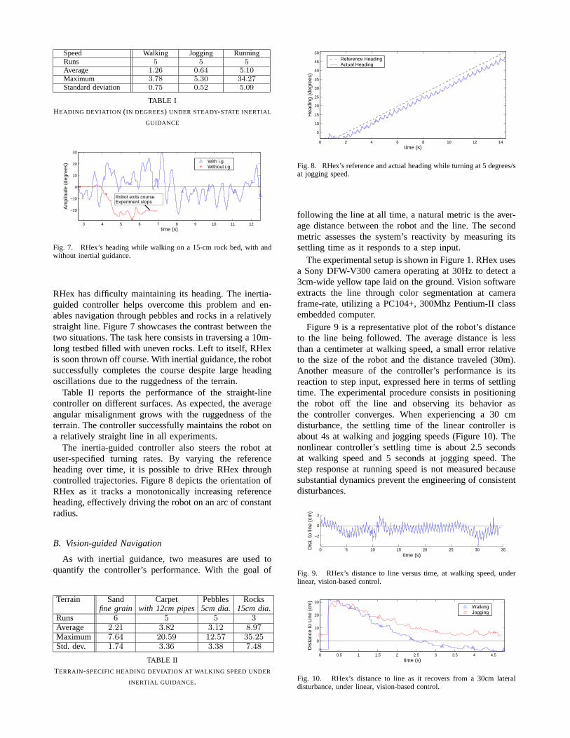
Speed Walking Jogging RunningRuns 5 5 5

Average 1.26 0.64 5.10

Maximum 3.78 5.30 34.27

Standard deviation 0.75 0.52 5.09

TABLE I

HEADING DEVIATION (IN DEGREES) UNDER STEADY-STATE INERTIAL

GUIDANCE

3 4 5 6 7 8 9 10 11 12

−20

−10

0

10

20

30

time (s)

Am

plitu

de (

degr

ees)

Robot exits courseExperiment stops

With i.g.Without i.g.

Fig. 7. RHex’s heading while walking on a 15-cm rock bed, withandwithout inertial guidance.

RHex has difficulty maintaining its heading. The inertia-guided controller helps overcome this problem and en-ables navigation through pebbles and rocks in a relativelystraight line. Figure 7 showcases the contrast between thetwo situations. The task here consists in traversing a 10m-long testbed filled with uneven rocks. Left to itself, RHexis soon thrown off course. With inertial guidance, the robotsuccessfully completes the course despite large headingoscillations due to the ruggedness of the terrain.

Table II reports the performance of the straight-linecontroller on different surfaces. As expected, the averageangular misalignment grows with the ruggedness of theterrain. The controller successfully maintains the robot ona relatively straight line in all experiments.

The inertia-guided controller also steers the robot atuser-specified turning rates. By varying the referenceheading over time, it is possible to drive RHex throughcontrolled trajectories. Figure 8 depicts the orientationofRHex as it tracks a monotonically increasing referenceheading, effectively driving the robot on an arc of constantradius.

B. Vision-guided Navigation

As with inertial guidance, two measures are used toquantify the controller’s performance. With the goal of

Terrain Sand Carpet Pebbles Rocksfine grain with 12cm pipes 5cm dia. 15cm dia.

Runs 6 5 5 3Average 2.21 3.82 3.12 8.97Maximum 7.64 20.59 12.57 35.25Std. dev. 1.74 3.36 3.38 7.48

TABLE II

TERRAIN-SPECIFIC HEADING DEVIATION AT WALKING SPEED UNDER

INERTIAL GUIDANCE .

0 2 4 6 8 10 12 14

5

10

15

20

25

30

35

40

45

50

time (s)

Hea

ding

(de

gree

s)

Reference HeadingActual Heading

Fig. 8. RHex’s reference and actual heading while turning at5 degrees/sat jogging speed.

following the line at all time, a natural metric is the aver-age distance between the robot and the line. The secondmetric assesses the system’s reactivity by measuring itssettling time as it responds to a step input.

The experimental setup is shown in Figure 1. RHex usesa Sony DFW-V300 camera operating at 30Hz to detect a3cm-wide yellow tape laid on the ground. Vision softwareextracts the line through color segmentation at cameraframe-rate, utilizing a PC104+, 300Mhz Pentium-II classembedded computer.

Figure 9 is a representative plot of the robot’s distanceto the line being followed. The average distance is lessthan a centimeter at walking speed, a small error relativeto the size of the robot and the distance traveled (30m).Another measure of the controller’s performance is itsreaction to step input, expressed here in terms of settlingtime. The experimental procedure consists in positioningthe robot off the line and observing its behavior asthe controller converges. When experiencing a 30 cmdisturbance, the settling time of the linear controller isabout 4s at walking and jogging speeds (Figure 10). Thenonlinear controller’s settling time is about 2.5 secondsat walking speed and 5 seconds at jogging speed. Thestep response at running speed is not measured becausesubstantial dynamics prevent the engineering of consistentdisturbances.

0 5 10 15 20 25 30 35

−2

0

2

Dis

t. to

line

(cm

)

time (s)

Fig. 9. RHex’s distance to line versus time, at walking speed,underlinear, vision-based control.

0 0.5 1 1.5 2 2.5 3 3.5 4 4.5

0

10

20

30

time (s)

Dis

tanc

e to

Lin

e (c

m)

WalkingJogging

Fig. 10. RHex’s distance to line as it recovers from a 30cm lateraldisturbance, under linear, vision-based control.

Speed Walking Jogging Runninglinear nonlinear linear nonlinear linear

Runs 5 5 5 5 5

Average 0.94 0.75 6.38 2.32 8.82

Maximum 17.68 6.48 13.11 7.07 31.08

Std. dev. 1.32 0.62 1.96 1.43 6.32

TABLE III

DISTANCE TO LINE (IN CM) UNDER LINEAR AND NONLINEAR

VISION-BASED CONTROL.

−0.5 −0.4 −0.3 −0.2 −0.1 0 0.1 0.2 0.3 0.4 0.5−0.5

−0.4

−0.3

−0.2

−0.1

0

0.1

0.2

0.3

0.4

0.5

w1

w2

simulationexperimentinitial condition

Fig. 11. Simulated and experimentalw-space trajectories for thenonlinear FOV respecting controller.

The performance results of the linear and nonlinearcontrollers are summarized in Table III. The maximumdeviation for the linear controller at walking speed issurprisingly high, but it is due to a single outlier distur-bance from which the controller promptly recovered. Theaverage distance to line when running is reasonable rela-tive to the slower speeds, but the large standard deviationreflects the swaying motions induced by the dynamics.The success is virtually 100% when walking and jogging,but only about 30% at running speed.

Figure 11 plots both simulated and experimental tra-jectories in thew1–w2 plane of the robot under the FOVrespecting controller. The dashed lines represent simulatedtrajectories, and the plot shows that the state stays withinthe parallelogram (FOV boundaries) for initial conditionswithin the parallelogram. The solid lines plot some exper-imental trajectories, demonstrating that the behavior of therobot somewhat matches the simulation predictions. Thecontroller is not tested for initial conditions near the FOVboundaries due to complexities of line detection in theseareas.

IV. CONCLUSION

This paper presented the first successful deployment ofsensor-guided behaviors on RHex. Controllers based onsimple motion models enable inertial straight-line loco-motion and visual line following. Experiments validatethe operational performance of the behaviors and provideinsight as to their limitation. These results constitute afirst step leading to sensor-guided operational autonomyfor dynamic legged robots.

Ongoing research is extending sensor-based capabilitiesto include robot state-estimation through visual regis-tration and inertial sensing. These efforts will enablerobot localization, online tuning of gait parameters andimproved locomotion notably at running speed and inunknown environments.

ACKNOWLEDGMENT

This work is supported by DARPA/ONR ContractN00014-98-1-0747.

V. REFERENCES

[1] Uluc Saranli.Dynamic Locomotion with a HexapodRobot. PhD thesis, University of Michigan, Septem-ber 2002.

[2] U. Saranli, M. Buehler, and D. E. Koditschek. RHex:A Simple and Highly Mobile Robot.InternationalJournal of Robotics Research, 20(7):616–631, July2001.

[3] S. Hutchinston, G. D. Hager, and P. I. Corke. Atutorial on visual servo control.IEEE Transactionson Robotics and Automation, 12(5), October 1996.

[4] I. H. Whang and T. W. Hwang. Horizontal way-point guidance design using optimal control.IEEETransactions on Aerospace and Electronic Systems,38(3):1116–1120, July 2002.

[5] T. Lee, K. Song, C. Lee, and C. Teng. Trackingcontrol of unicycle-modeled mobile robots using asaturation feedback controller.IEEE Transactionson Control Systems Technology, 9:305–318, March2001.

[6] F. Diaz del Rio., G. Jimenez, J. L. Sevillano, S. Vi-cente, and A. Civit Balcells. A generalization ofpath following for mobile robots. In1999 IEEE In-ternational Conference on Robotics and Automation,pages 7–12, Detroit, MI, May 1999.

[7] B. Kwolek, T. Kapuscinski, and M. Wysocki. Vision-based implementation of feedback control of unicy-cle robots. InProceedings of the First Workshop onRobot Motion and Control, pages 101–106, Piscat-away, NJ, 1999. IEEE.

[8] Y. Ma, J. Kovsecka, and S. Sastry. Vision guidednavigation for a nonholonomic mobile robot. InD. Kriegman, G. Hager, and A. S. Morse, editors,Lecture Notes in Control and Information Sciences237, pages 134–145. Springer, 1998.

[9] P. Murrieri, D. Fontanelli, and A. Bicchi. Visual-servoed parking with limited view angle. InB. Siciliano and P. Dario, editors,ExperimentalRobotics VIII, STAR 5, pages 265–274. Springer-Verlag, Berlin Heidelberg, 2003.

[10] J. Schmitt and P. Holmes. Mechanical models forinsect locomotion: Dynamics and stability in thehorizontal plane - I. Theory.Biological Cybernetics,83:501–515, April 2000.

[11] D. Maiwand. System identification, using vision-based localisation, for a hexapod robot. Master’sthesis, Carnegie Mellon University, May 2003.