Embed Size (px)
Citation preview
Inflation Dynamics and the Great Recession
Laurence Ball and Sandeep Mazumder
WP/11/121
© 2011 International Monetary Fund WP/11/121
IMF Working Paper
Research Department
Inflation Dynamics and the Great Recession
Prepared by Laurence Ball and Sandeep Mazumder*
Authorized for distribution by Prakash Loungani
June 2011 Abstract
* This is a revised version of a paper that was prepared for the March 2011 Brookings Panel on Economic Activity. We are grateful for excellent research assistance from Indra Astrayuda, Kue Peng Chuah, Xu Lu, Prathi Seneviratne, and Hou Wang, and for suggestions from the editors, Karen Dynan, Jon Faust, Robert Gordon, Jeremy Rudd, James Stock, Eric Swanson, Jonathan Wright, and participants at the Brookings Panel. We are also very grateful to Brent Meyer for assistance with the Cleveland Fed’s data on inflation. Ball: Visiting Scholar, International Monetary Fund, [email protected]; and Department of Economics, Johns Hopkins University, [email protected]. Mazumder: Department of Economics, Wake Forest University, [email protected] .
This paper examines inflation dynamics in the United States since 1960, with a particular focus on the Great Recession. A puzzle emerges when Phillips curves estimated over 1960-2007 are ussed to predice inflation over 2008-2010: inflation should have fallen by more than it did. We resolve this puzzle with two modifications of the Phillips curve, both suggested by theories of costly price adjustment: we measure core inflation with the median CPI inflation rate, and we allow the slope of the Phillips curve to change with the level and vairance of inflation. We then examine the hypothesis of anchored inflation expectations. We find that expectations have been fully “shock-anchored” since the 1980s, while “level anchoring” has been gradual and partial, but significant. It is not clear whether expectations are sufficiently anchored to prevent deflation over the next few years. Finally, we show that the Great Recession provides fresh evidence against the New Keynesian Phillips curve with rational expectations.
JEL Classification Numbers:E31 Keywords: Inflation, Phillips curve, Great Recession Author’s E-Mail Address: [email protected] , [email protected]
This Working Paper should not be reported as representing the views of the IMF.
The views expressed in this Working Paper are those of the author(s) and do not necessarily represent those of the IMF or IMF policy. Working Papers describe research in progress by the author(s) and are published to elicit comments and to further debate.
2
Contents Pages
1. Introduction ............................................................................................................................ 4 2. A Simple Phillips Curve and a Puzzle ................................................................................... 7
2.1 The Philips Curve ............................................................................................................ 7 2.2 The Puzzle ........................................................................................................................ 9
3. Measuring Core Inflation ..................................................................................................... 10 3.1 Measuring Supply Shocks.............................................................................................. 10 3.2 From Supply Shocks to Core Inflation .......................................................................... 11 3.3 Measuring Median Inflation .......................................................................................... 12 3.4 Some New Evidence ...................................................................................................... 13 3.5 Median Inflation During the Great Recession ............................................................... 14
4. A Phillips Curve with a Time-Varying Slope ...................................................................... 14 4.1 Estimates of a Time-Varying Slope ............................................................................... 15 4.2 Determinants of the Slope .............................................................................................. 16 4.3 Estimating Constant Slopes for Subsamples.................................................................. 17 4.4 The Great Recession and the Risk of Deflation ............................................................. 19 4.5 Robustness ..................................................................................................................... 20
5. Anchored Expectations? ...................................................................................................... 20 5.1 Shock Anchoring ........................................................................................................... 21 5.2 Level Anchoring ............................................................................................................ 22 5.3 Dynamic Forecasts ......................................................................................................... 24
6. The New Keynesian Phillips Curve ..................................................................................... 25 7. Conclusion ........................................................................................................................... 28
Appendices
A. Appendix .............................................................................................................................. 30 A.1. Longer Lags ................................................................................................................. 30 A.2. The Stock-Watson Unemployment Gap ..................................................................... 30 A.3. A Nonlinear Phillips Curve ......................................................................................... 31 A.4. Productivity Growth .................................................................................................... 32 A.5. Estimating A Time-Varying NAIRU .......................................................................... 32 A.6. Supply Shocks ............................................................................................................. 33
References ....................................................................................................................................... 35 Tables
1. Phillips Curve Estimated from 1960:1 to 2007:4 ................................................................ 40 2. Phillips Curve with Level and Variance of Inflation ........................................................... 41 3. Phillips Curve for Core Inflation ......................................................................................... 42 4. Shock Anchoring in the Phillips Curve ............................................................................... 43 5. New Keynesian Phillips Curve Results ............................................................................... 44 A.1. Variations on Basic Phillips Curves................................................................................... 45
Figures
1. 4-Quarter Moving Averages of Dynamics Forecasts of Inflation for 2008 to 2010 Based on 1960:1-2007:4 Regression ................................................................................... 46
3
Contents Pages
2. Median CPI and XFE CPI Inflation Rates, 1983:2-2010:4 ................................................. 47 3. Time-Varying αt from Phillips Curve, 1960:1-2010:4 ........................................................ 48 4. Permanent Component of Median CPI Inflation vs. Time-Varying α ................................. 49 5. Dynamic Forecasts of Median CPI Inflation Based for 2008 to 2010 on 1985:1-
2007:4 .................................................................................................................................. 50 6. Dynamic Forecasts of ZFE CPI Inflation Based for 2008 to 2010 on 1985:1-2007:4
Regression ............................................................................................................................ 51 7. 4-Quarter Moving Averages of Dynamic Forecasts of Median CPI Inflation for 2008
to 2010 ................................................................................................................................. 52 8. 4-Quarter Moving Averages of Dynamic Forecasts of XFE CPI Inflation for 2008 to
2010...................................................................................................................................... 52 9. 4-Quarter Moving Averages of Dynamic Forecasts of Median CPI Inflation for 2011
to 2013 Based on 1985:1-2010:4 Regression ...................................................................... 53 10. Level Anchoring Based on SPF4Q=δt2.5+(1- δt)
(πt-1+πt-2+πt-3+πt-4), 1985:1-2010:4 ....... 53
11. Level Anchoring Based on πt= δt 2.5+(1-δt)
(πt-1+πt-2+πt-3+πt-4)+α(u-
), 1985:1-2010:4 .................................................................................................................................. 54
12. Level Anchoring based on πt=δt2.5++(1-δt)
(πt-1+πt-2+πt-3+πt-4)+α(y-
), 1985:1-2010:4 .................................................................................................................................. 54
13. 4-Quarter Moving Averages of Dynamic Forecasts of Median CPI Inflation for 2008 to 2010 Based on Phillips Curve with Anchoring, 1985:1-2007:4 ...................................... 55
14. 4-Quarter Moving Averages of Dynamic Forecasts of Median CPI Inflation for 2011 to 2013 Based on Phillips Curve with Anchoring, 1985:1-2010:4 ...................................... 55
15. Labor Income Share vs. Unemployment Gap (Annual Averages), 1985-2010 ................... 56 A1. 4-Quarter Moving Averages of Dynamic Forecasts of Median CPI Inflation for 2008 to 2010 Based on Gordon (2011) ............................................................................................... 56
1 Introduction
In his Presidential Address, Friedman (1968) presented a theory of the short run behavior of
inflation. In Friedman’s theory, inflation depends on expected inflation and the gap between
unemployment and its natural rate. Friedman also suggested that “unanticipated inflation
generally means a rising rate of inflation”–in other words, that expected inflation is well-proxied
by past inflation. These assumptions imply an accelerationist Phillips curve that relates the
change in inflation to the unemployment gap.
In the decades since Friedman’s work, his model has been a workhorse of macroeconomics.
Researchers have refined the model extensively; two of the numerous examples are Gordon
(1982, 1990)’s introduction of supply shocks and Staiger et al. (1997)’s modeling of a time-
varying natural rate. Economists have debated how well the accelerationist Phillips curve fits
the data, some declaring the equation’s demise and others reporting that “The Phillips Curve
Is Alive and Well” (Fuhrer, 1995).
Debate over the Phillips curve has gained momentum during the U.S. economic slump that
began in 2007. Some economists see a puzzle: inflation has not fallen as much as a traditional
Phillips curve predicts, given the high level of unemployment. For example, in September 2010,
John Williams (now president of the San Francisco Fed) said:
“The surprise [about inflation] is that it’s fallen so little, given the depth and duration of the
recent downturn. Based on the experience of past severe recessions, I would have expected infla-
tion to fall by twice as much as it has.”
In addition to analyzing the recent behavior of inflation, economists are debating its likely
path in the future. If the accelerationist Phillips curve is accurate, then high unemployment
implies a substantial risk that inflation will fall below zero. Yet many economists argue that
deflation is unlikely, primarily because the Federal Reserve’s commitment to a low but positive
inflation rate has “anchored” inflation expectations. According to Bernanke (2010),
2
“Falling into deflation is not a significant risk for the United States at this time, but that is
true in part because the public understands that the Federal Reserve will be vigilant and proac-
tive in addressing significant further disinflation.”
This paper contributes to the debate over past and prospective inflation in several steps. We first
show why it is easy to view recent inflation behavior as puzzling. We estimate accelerationist
Phillips curves with quarterly data for the period 1960-2007, measuring inflation with either
the CPI or the CPI less food and energy (XFE), the standard measure of “core” inflation. We
use the estimated equation and the path of unemployment over 2008-2010 to produce dynamic
forecasts of inflation. In these forecasts, a four-quarter moving average of core inflation falls to
-4.3% in 2010Q4. In reality, four-quarter core inflation was 0.6% in 2010Q4. A simple Phillips
curve predicts a deflation that did not occur.
We show, however, that two simple modifications of the Phillips curve eliminate this puzzle.
They produce a specification that fits the entire period since 1960, including the Great Reces-
sion. Both modifications are suggested by theory, specifically, models of costly nominal price
adjustment from the 1980s and 1990s.
First, following Bryan and Cecchetti (1994), we measure core inflation with a weighted
median of price changes across industries. This approach is motivated by price-adjustment
models in which unusually large relative-price changes cause movements in aggregate inflation.
Median inflation fell by more than XFE inflation from 2007 to 2010, reflecting a higher initial
level (in 2007, median inflation was about 3% and XFE inflation was 2%). The relatively large
fall in median inflation reduces the gap between forecasted and actual inflation.
Second, following Ball, Mankiw, and Romer (1988), we allow the slope of the Phillips curve–
the coefficient on unemployment–to vary over time. In the Ball-Mankiw-Romer theory, the
Phillips curve steepens if inflation is high and/or variable, because these conditions reduce nom-
inal price stickiness. U.S. time series evidence strongly supports this prediction; in particular,
the Phillips curve has been relatively flat in the low-inflation period since the mid-1980s. A
flatter Phillips curve reduces the forecasted fall in inflation over 2008-2010. When we account
for this effect and measure core inflation with the median price change, forecasted four-quarter
3
inflation in 2010Q4 is 0.3%, close to the actual level of 0.5%.
After presenting these results, we turn to the idea of anchored expectations. We distinguish
between “shock anchoring,” which means that expectations do not respond to supply shocks,
and “level anchoring,” which means that expectations stay fixed at a certain level regardless of
any movements in actual inflation. We assume this level is 2.5% for core CPI inflation (which
corresponds to about 2% for core PCE inflation). Based on the behavior of actual inflation and of
expectations (as measured by the Survey of Professional Forecasters), we find that expectations
have been fully shock-anchored since the 1980s. Level anchoring has been gradual and partial,
but significant. According to our estimates, the fraction of a change in core inflation that is
passed into expectations fell from roughly one in 1985 to between 0.4 and 0.7 in 2010.
Following our analysis of recent inflation, we forecast inflation over 2011-2013, using our
estimates of the Phillips curve through 2010 and CBO forecasts of unemployment and output
over the forecast period. Here, the results depend crucially on whether we incorporate anchored
expectations into our equation. Our basic accelerationist specification, while explaining why
inflation is currently positive, predicts that deflation is on the way. In contrast, the degree of
expectation anchoring estimated for 2010 is high enough to keep inflation positive. We are not
confident in this forecast, however, because it assumes that expectations will stay anchored at
2.5% for several years when actual inflation is less than 1%.
Most of this paper examines Phillips curves in which expected inflation depends on past
inflation and possibly the Federal Reserve’s target. A large literature since the 1990s studies an
alternative, the “New Keynesian” Phillips curve based on rational expectations and the Calvo
(1983) model of staggered price adjustment. The last part of this paper asks whether the New
Keynesian Phillips curve helps explain recent inflation behavior; the answer is no. Indeed, the
last few years provide fresh evidence of the poor empirical performance of the model, especially
the Gali and Gertler (1999) version in which marginal cost is measured with labor’s share of
income. This specification produces the counterfactual prediction of rising inflation over 2008-
2010.
Parts of our analysis overlap with other recent research on the Phillips curve, such as Fuhrer
et al. (2009), Fuhrer and Olivei (2010), and Stock and Watson (2008, 2010). We compare our
4
results to previous work throughout the paper. One difference from Stock and Watson’s work is
that they focus on forecasting inflation in real time. In seeking to understand inflation behavior,
we freely use information that is not available in real time, such as the 2011 CBO series for the
natural rate of unemployment.
2 A Simple Phillips Curve and a Puzzle
We first introduce a conventional Phillips curve, then show that it predicts a large deflation over
2008-2010.
2.1 The Phillips Curve
Milton Friedman’s Phillips curve can be expressed as
πt = πet + α(u− u∗)t + ǫt (1)
where π is annualized quarterly inflation, πe is expected inflation, u is unemployment, u∗ is the
natural rate, and ǫ is an error term that we assume is uncorrelated with u − u∗. A common
variant of this equation replaces u−u∗ with the gap between actual and potential output. Since
Friedman wrote, theorists have derived equations that are broadly similar to (1) from models in
which price setters have incomplete information (e.g. Lucas, 1973; Mankiw and Reis, 2002) or
nominal prices are sticky (e.g. Roberts, 1995).1
We follow a long tradition in applied work that assumes backward-looking expectations:
expected inflation is determined by past inflation. Specifically, we assume that expected inflation
1The assumption that u−u∗ is uncorrelated with the error in the Phillips curve, implying that OLS estimatesof the equation are unbiased, is standard in the literature but rarely examined. We interpret the error term assummarizing the effects of relative price changes, which influence inflation when some nominal prices are sticky(see Section 3). We assume that these relative-price effects are uncorrelated with the aggregate variable u− u∗.We maintain this assumption when π is a measure of core inflation, which strips away effects of relative pricechanges but does so imperfectly. In this case, the error summarizes the relative-price effects that are not removedfrom core inflation.
This approach to identification ignores the problem of measurement error. The variable u is an imperfectmeasure of the activity variable in the Phillips curve, and u∗ is an imperfect measure of the natural rate. Theseproblems bias our estimates of the coefficient α toward zero. Future work should investigate the size of this biasand more generally the identification problem for the Phillips curve.
5
is the average of inflation in the past four quarters. In this case, equation (1) becomes
πt =1
4(πt−1 + πt−2 + πt−3 + πt−4) + α(u− u∗)t + ǫt (2)
This equation is a special case of Phillips curves estimated by Gordon and Stock-Watson, which
generally include lags of unemployment and lags of inflation with unrestricted coefficients (except
for the accelerationist assumption that the coefficients sum to one). We keep our specification
parsimonious along this dimension to enrich it more easily along others (for example, by allow-
ing time-variation in the coefficient α). We examine versions of equation (2) with richer lag
structures as part of our robustness checks.
The structure of inflation lags in equation (2) implies that a one-percentage-point increase
in unemployment for one quarter changes inflation in the long run by 0.4 times the coefficient
α. The long run effect of one point of unemployment sustained for a year is 1.6 times α.
The structure of inflation lags in equation (2) implies that a one-percentage-point increase
in unemployment for one quarter changes inflation in the long run by 0.4 times the coefficient
α. The long run effect of one point of unemployment sustained for a year is 1.6 times α.2
Our empirical work requires a series for the natural rate of unemployment or for potential
output. For most of our analysis, we use estimates of these variables from the Congressional
Budget Office; as a robustness check, we estimate a path for the natural rate using a technique
from Staiger et al. (1997). The CBO natural-rate series is similar to estimates from other sources:
the natural rate rises modestly in the 1960s and 1970s, from about 5.5% to 6.3%, then falls to
5.0% in the 1990s. It remains at 5.0% through 2007, then rises slightly to 5.2% in 2010.
Since Gordon (1982), many empirical researchers add “supply shocks” to the Phillips curve.
Others seek to filter supply shocks out of the dependent variable with measures of core inflation.
The most common supply shocks are changes in the relative prices of food and energy, and the
standard core-inflation measure is inflation less food and energy. Most of this paper examines
core inflation, but we experiment with alternative measures of this variable.
2The easiest way to derive this result is to numerically calculate the path of inflation following an increase inunemployment.
6
2.2 The Puzzle
We now take our first pass at estimating the Phillips curve. We want to know whether equation
(2) fits inflation behavior since 1960, and especially whether anything has changed during the
Great Recession. The starting date of 1960 is based on Barsky (1987), who finds a regime change
in the univariate behavior of inflation at that point, from a stationary process to an IMA(1,1)
(a process that still captures inflation behavior, albeit with time-varying parameters, according
to Stock and Watson, 2010).
We estimate equation (2) for the period 1960-2007, ending the sample at the start of the Great
Recession. We examine two measures of inflation, one derived from the CPI (total inflation) and
one from the CPI excluding food and energy (XFE inflation). In each case we average monthly
data on the price level to create quarterly price levels, then compute annualized percentage
changes from quarter to quarter. For each inflation variable, we estimate a Phillips curve that
includes the unemployment gap and one that includes the output gap.
Table 1 presents our regression results. For both measures of inflation, the coefficients
on unemployment are about -0.5 and are highly significant statistically (t > 5). The output
coefficients are around 0.25, which accords with the unemployment coefficients and Okun’s Law.
Recall that one point-year of unemployment or output changes long-run inflation by 1.6
times the variable’s coefficient. For example, in the equation with XFE inflation and output,
the estimated coefficient implies an effect of approximately (1.6)(0.25) = 0.4 percentage points.
Equivalently, the sacrifice ratio for reducing inflation is 10.4 = 2.5. This result is in the ballpark
of previous estimates of U.S. sacrifice ratios (e.g., Ball, 1994).
Next, we perform dynamic forecasts of inflation over 2008-2010. We start with actual infla-
tion through 2007 and feed the path of unemployment over 2008-2010 into the estimated Phillips
curves in Table 1. Figure 1 compares the forecasted and actual levels of total inflation (Panel A)
and XFE inflation (Panel B). We present four-quarter moving averages so we can ignore some
of the transitory fluctuations in quarterly data.
Figure 1 illustrates why some economists think the Phillips curve has broken down recently.
Actual XFE inflation, for example, fell from 2.6% in 2007Q4 to 0.4% in 2010Q4. In the dynamic
forecasts, XFE inflation falls to -5.5% for the unemployment equation and -4.1% for the output
7
equation. The pre-2008 Phillips curve predicts a deflation that didn’t occur.
3 Measuring Core Inflation
Here we compare alternative measures of core inflation. We start by discussing supply shocks,
the fluctuations in inflation that core measures are meant to filter out.
3.1 Measuring Supply Shocks
The Phillips curve in much applied work is Gordon’s “triangle model.” It explains total inflation
with three factors: expected inflation, aggregate activity, and supply shocks. The most common
measures of supply shocks are changes in the relative prices of food and energy. Since the 1970s,
these variables have added greatly to the R2s of estimated Phillips curves.
Yet, theoretically, it is not obvious why certain relative prices should influence inflation–why
it depends on food and energy prices rather than, say, the prices of clothing and home appliances.
As Friedman (1975) asked, “Why should the average level of prices be affected significantly by
changes in the price of some things relative to others?”
A number of economists answer this question with models of nominal price stickiness. Many,
ranging from the Dornbusch and Fischer (1990) text to Blanchard and Gali (2008), assume that
food and energy prices are flexible and other prices are sticky. In this setting, a shock that
raises the relative prices of food and energy does so by increasing their nominal prices while
other prices stay constant. This pattern of adjustment implies an increase in the aggregate price
level.
Ball and Mankiw (1995) present a theory of supply shocks based on a different sticky-price
model. Rather than assume certain industries have sticky or flexible prices, Ball and Mankiw
make price adjustment endogenous. Firms receive shocks to their equilibrium relative prices and
choose whether to pay a menu cost and adjust prices. In each period, the firms that receive the
largest shocks are most likely to adjust.
The upshot is that inflation depends on the distribution of price changes across industries.
If the distribution is skewed to the right, for example, that means many firms have desired
8
price increases that are large enough to trigger adjustment, and relatively few have large enough
negative shocks to adjust. As a result, the aggregate price level rises. Based on this result,
Ball and Mankiw measure supply shocks with the skewness of relative price changes and other
measures of asymmetry.
In practice, the competing measures of supply shocks–food and energy prices and asymme-
tries in price distributions–are positively correlated. The reason is that, in many periods, large
changes in food and energy prices create large tails in price distributions. Yet there is enough
independent variation in supply-shock measures to see which are most closely related to infla-
tion. For the period 1949 to 1989, Ball and Mankiw show that only price-change asymmetries,
not changes in food and energy prices, are significant when both are included in a Phillips curve.
3.2 From Supply Shocks to Core Inflation
We define core inflation as the part of inflation not explained by supply shocks, but rather
by expected inflation and economic activity–the two other parts of the triangle. With this
definition, one can measure core inflation by removing the effects of supply shocks from total
inflation. This approach follows common practice. When researchers measure supply shocks
with changes in food and energy prices, they measure core inflation with XFE inflation, which
strips away the direct effects of food and energy.
If supply shocks are asymmetries in the distribution of price changes, then a measure of
core inflation should eliminate the effects of these asymmetries. A simple measure, proposed by
Bryan and Cecchetti (1994), is the weighted median of price changes across industries (median
inflation).
Researchers sometimes evaluate core inflation measures by their ability to forecast future
inflation. In theory, core inflation as we define it might not be a good forecaster. A rise in total
inflation caused by a supply shock might raise expected inflation, which in turn raises future
inflation; in that case, total inflation would be a better forecaster than core inflation. In practice,
however, papers such as Sommer (2004) and Hooker (2002) find that, since the 1980s, supply
shocks have not fed strongly into future inflation; thus, core inflation is a good forecaster. We
return to this point when we discuss the anchoring of inflation expectations.
9
Smith (2004) compares median inflation and XFE inflation as forecasters of total inflation
over 1984-1997. She finds that forecasts based on median inflation are more accurate.
3.3 Measuring Median Inflation
The Federal Reserve Bank of Cleveland maintains a monthly series for median inflation that
begins in 1968. The economy is disaggregated into about forty industries (the number rises
from 36 to 45 over time), and core inflation is measured by the weighted median of industry
inflation rates, using the industries’ weights in the CPI.
The data include an “original” weighted median for 1968-2007 and a “revised” median for
1983 to the present. The main difference is that the original data include owner’s equivalent
rent (OER) as the price for one large industry, while the revised data include OER for four
geographic regions. This revision makes some difference because the change in OER (in the
original data) or one of the regional changes (in the revised data) is the median price change
for around half of the observations. For the period when the two median series overlap, the
differences are modest, although the original series shows somewhat greater monthly volatility.
For more documentation of the Cleveland Fed data, see Bryan and Pike (1991) and Bryan et al.
(1997).3
We compute quarterly data for median inflation that matches the timing of our quarterly
series for total and XFE inflation. We first use the monthly median inflation rates from the
Cleveland Fed to construct a monthly series for price levels. Then we average three months to
get a quarterly price level, and compute annualized percentage changes in that variable.4
The time-aggregation of median inflation is not straightforward. Instead of our approach, one
could measure the median of quarterly price changes across industries; in principle, this median
3Some economists (including one of our discussants) question median CPI as an inflation measure because themedian price change in the Cleveland Fed data is often one of the regional OERs. It is not clear to us why thevalidity of the Cleveland Fed’s approach depends on which industry is the median. Nonetheless, as a robustnesscheck, we have constructed median non-housing inflation by discarding the regional OERs and computing themedian price change for all other industries. A four-quarter average of this series falls by 2.1 percentage pointsbetween 2007Q4 and 2010Q4 (from 3.1% to 1.0%); the fall in the Cleveland Fed’s median, 2.6 percentage points,is somewhat larger. Yet housing prices have a greater effect on the other leading measure of core inflation, XFE.This variable falls by 1.7 percentage points between 2007Q4 and 2010Q4; if the OERs are removed along withfood and energy, the resulting inflation measure falls by only 0.9 percentage points.
4The Cleveland Fed website provides a different measure of quarterly inflation: the average of median inflationover the three months of the quarter.
10
might differ greatly from the quarterly variable that we construct from monthly medians. This
non-robustness arises because the median is not a linear function of industry price changes.
Future research might compare measures of median inflation based on different frequencies for
industry-level data.
3.4 Some New Evidence
We present one new piece of evidence on the measurement of core inflation. Both expected
inflation and the activity gap are persistent series, and hence the part of inflation they determine–
core inflation–is persistent. One should not expect significant transitory movements in quarterly
core inflation. Therefore, one criterion for judging core inflation measures is the extent that their
movements are permanent or transitory.
We implement this idea with Stock and Watson (2007)’s procedure for decomposing inflation
into permanent and transitory components. Stock and Watson assume that inflation is the
sum of a permanent, random-walk component and a transitory, white-noise component. This
specification implies that aggregate inflation follows an IMA(1,1) process. Stock and Watson
allow the variances of the permanent and transitory shocks to change over time. They estimate
series for the permanent component of inflation and the variances of the two shocks.
We apply the Stock-Watson procedure to the two competing measures of core inflation,
XFE inflation and median inflation. Figure 2 shows the quarterly series for these two variables
and their estimated permanent components. The sample starts in 1983Q2, when the “revised”
median data begin. The divergences between total and permanent inflation–the transitory
shocks–are smaller when inflation is measured by median inflation. This difference is especially
pronounced in the 2000s, when median inflation appears to have almost no transitory component.
These results bolster the case for measuring core inflation with the median.
The two core measures behave differently because price changes that are large relative to
aggregate inflation–annualized monthly changes of 20% or more–occur frequently in industries
besides food and energy. Some of these industries, such as used cars and lodging away from
home, may be affected indirectly by energy prices. Women’s apparel is an example of a non-
energy-related industry with volatile prices. Large price changes in all these industries cause
11
transitory movements in XFE inflation, but their effects are filtered out by the Cleveland Fed
median.
3.5 Median Inflation During the Great Recession
An important fact for our purposes is that median inflation has fallen somewhat more than
XFE inflation during the Great Recession. Over the period from 2007Q4 to 2010Q4, the four-
quarter moving average of median inflation fell from 3.1% to 0.5%, while the four-quarter moving
average of XFE inflation fell from 2.3% to 0.6%. Median inflation fell by more primarily because
it started at a higher level.
Median inflation was relatively high in 2007 because the distribution of price changes was
left-skewed during many months of the year. Left-skewness resulted from large price decreases
in various industries. In March 2007, for example, the prices of jewelry and watches fell at an
annualized rate of 30%, car and truck rental fell 22%, and lodging away from home fell 13%.
These price decreases reduced XFE inflation but not median inflation.
The relatively large fall in the median goes in the right direction for reducing the divergence
between actual and forecasted inflation over 2008-2010. Yet changing the definition of core
inflation is far from enough to resolve the puzzle in Figure 1. We also need another modification
of the Phillips curve, which we turn to next.
4 A Phillips Curve With a Time-Varying Slope
As we have discussed, models of costly price adjustment provide a rationale for measuring core
inflation with median inflation. These models also imply time variation in the slope of the
Phillips curve. As shown by Ball, Mankiw, and Romer (1988), if nominal price adjustment
is costly, firms choose to adjust more frequently when the level of inflation is higher and the
variance of inflation is higher. More frequent nominal adjustment makes the aggregate price level
more flexible, steepening the Phillips curve. That is, the unemployment coefficient α increases
in absolute value with the level and variance of inflation.
Ball, Mankiw, and Romer present international evidence supporting their model. In a cross-
12
country regression for 43 countries, the average level of inflation has a strong effect on the
Phillips-curve slope. DeFina (1991) finds a similar effect in U.S. time series data.
Here we document time-variation in the Phillips curve slope from 1960 through 2010. We
then show that this variation is tied closely to the level and variance of inflation, as predicted
by theory. Finally, we explore the implications for inflation during the Great Recession and in
the future.
4.1 Estimates of a Time-Varying Slope
We generalize the basic Phillips curve, equation (2), as follows:
πt =1
4(πt−1 + πt−2 + πt−3 + πt−4) + αt(u− u∗)t + ǫt (3)
αt = αt−1 + ηt
where ǫt and ηt are white noise errors with variances V and W respectively. This specification
allows the coefficient α to vary over time; specifically, it follows a random walk.
Equation (3) is a standard regression equation with a time-varying coefficient. We estimate
two versions of this specification. In the first, we assume a value for the ratio of the two shock
variances, V and W . With this restriction, we can estimate the path of αt with the Kalman
smoother. We choose V/W to create a degree of smoothness in αt that appears plausible. Our
intuition is that firms’ price-setting policies, which determine the Phillips curve slope, do not
vary greatly from quarter to quarter. DeVeirman (2007) uses a similar approach to estimate a
time-varying Phillips curve slope for Japan.
In the second version of our procedure, we estimate the shock variances V and W along
with the path of αt. As suggested by Harvey (1989, Ch. 3) and Wright (2010), we choose the
two variances to maximize the likelihood produced by the Kalman smoother. This method is
roughly equivalent to choosing the variances to minimize one-step-ahead forecast errors from
the model.5
We estimate equation (3) for the period 1960-2010. For observations over 1984Q2-2010Q4,
5As a robustness check, we also estimate a time-varying α with a simpler technique: rolling regressions withfive-year windows. The qualitative results are the same.
13
we measure inflation with the Cleveland Fed’s revised median. For 1968Q2-1984Q1, we use the
original median. For 1960Q1-1968Q1, when the median is not available, we use XFE inflation.
We obtain similar results when we use XFE inflation for the entire sample; the measurement of
core inflation is not critical for our results about the Phillips curve slope.
Figure 3 presents estimates of the path of αt, along with two-standard-error bands. Panel
A shows the results when the two shock variances are estimated freely, and Panel B imposes
the restriction that V/W , the ratio of the variances of ǫ and η, is 100. (Higher values of V/W
produce smoother series for α, and lower values produce more variable series.)
The two panels show the same broad trends in α: the estimated parameter falls from near
zero in 1960 to around -1 in the early 1970s, fluctuates around this level until 1980, then rises
sharply and levels off in the neighborhood of -0.2. In the period since the mid-1980s–the second
half of the sample–the estimated α is quite stable. Given the standard errors, there is no evidence
against a constant α over 1985-2010.
4.2 Determinants of the Slope
Theory predicts that α is determined by the level and variance of inflation. Figure 4 tests this
idea by comparing the estimated path of α (smoothed with V/W = 100, and presented on
an inverted scale) to two series generated by the Stock-Watson IMA(1,1) model: the level of
permanent inflation, and the standard deviation of the sum of permanent and transitory shocks.
The results in Figure 4 are striking: the measures of the level and variability of inflation
move together, and the estimated path of α follows them closely. These results strongly confirm
the predictions of sticky-price models about time-variation in α. In particular, the high and
variable inflation of the 1970s and early 80s created a steep Phillips curve; the curve was flatter
before 1973 and after the Volcker disinflation, when inflation was relatively low and stable.
We can also capture these ideas with a regression. We assume that the coefficient α is a
linear function of the other two series in Figure 4: αt = (a0+a1πt+a2σt), where π and σ are the
level of permanent inflation and the standard deviation of shocks . Substituting this assumption
14
into equation (3) yields
πt =1
4(πt−1 + πt−2 + πt−3 + πt−4) + a0(u− u∗)t + a1πt(u− u∗)t + a2σt(u− u∗)t + ǫt (4)
Table 2 presents estimates of this equation for 1960-2010 and compares them to an equation
with a constant α. We measure πt and σt in two different ways: with the quarterly series for these
parameters and with four-quarter moving averages. In both cases, the joint significance of the π
and σ terms is high (p < 0.01). Unfortunately, the collinearity between the two variables makes
it difficult to distinguish their individual roles: only π is significant in one of our specifications,
and only σ is significant in the other.
Many other authors present evidence that the Phillips-curve slope has changed over time;
examples include Roberts (2006) and Mishkin (2007). These authors focus on the decline in the
unemployment coefficient since the 1980s, and generally give a different explanation from ours:
they suggest that a flatter Phillips curve reflects an anchoring of inflation expectations. We
question this view on two grounds. First, the theory is weak. When the Phillips curve is derived
from microeconomic foundations, the unemployment coefficient is determined by the slope of
marginal cost and the frequency of price adjustment (Roberts, 1995). Anchoring influences
the expected-inflation term in the equation–an effect we examine in Section 5–but not the
unemployment coefficient. Second, the common explanation for anchoring is that Fed policy has
become more credible since the Volcker disinflation. This story does not explain why the Phillips
curve was flat in the 1960s as well as the post-Volcker era, a result that the Ball-Mankiw-Romer
model does explain.
4.3 Estimating Constant Slopes for Subsamples
As noted above, the data suggest that α has been close to a constant since the early 1980s,
when inflation stabilized at a low level. Assuming a constant α will make it more tractable to
enrich the model along other dimensions. Therefore, we assume a constant α starting in 1985Q1,
roughly the end of the disinflation and high unemployment of the early 80s. We examine periods
15
ending in 2007Q4 and 2010Q4 to check for effects of the Great Recession.6
For comparison, we also estimate a constant α for the periods 1960-1972 and 1973-1984.
Figure 4 suggests some variation in α within these periods, but the statistical significance of
this variation is borderline. α is generally low in absolute value during the first period and high
during the second.
Table 3 presents estimates of α for each of the periods. We estimate equations with the output
gap as well as the unemployment gap, and with XFE inflation as well as median inflation. For
the first period, 1960-1972, we only examine XFE inflation, because median inflation is not
available for most of the period. We measure median inflation with the original Cleveland Fed
series for 1973-84 and with the revised series for the periods beginning in 1985.7
For the first three time periods in the table–covering the years from 1960 to the eve of the
financial crisis–the estimated coefficients are similar for the two inflation measures. The unem-
ployment coefficient is around -0.2 or -0.25 for both 1960-1972 and 1985-2007. The coefficient
is around -0.7 for the 1973-1984 period of high and volatile inflation. The coefficients on output
are about -0.5 times the unemployment coefficients, as suggested by Okun’s Law.
As before, multiplying the output coefficient by 1.6 yields the long-run effect on inflation of
a one percent output gap for a year. For 1985-2007, with inflation measured by the median, this
effect is (1.6)(0.11) = 1.76. The sacrifice ratio is 1/(0.176), or about 6.
Extending the final sample from 2007 to 2010 has different effects for the different core
inflation measures. For XFE inflation, the coefficients decline substantially in absolute value;
for median inflation, the coefficients fall by less (when activity is measured by the unemployment
gap) or not at all (for the output gap). This difference suggests greater stability in the Phillips
curve when inflation is measured by the median, a result we will confirm with dynamic forecasts.
6The results do not change significantly if start the sample a year or two later. They are less robust when wemove the start date earlier, with observations before 1985 proving influential.
7Note that, in these regressions, we use the original median through 1985 even though the revised medianis available starting in 1983Q2. This choice ensures that our measure of median inflation is consistent over the1973-1984 subsample.
16
4.4 The Great Recession and the Risk of Deflation
We now revisit the puzzle of inflation over 2008-2010. Figures 5 and 6 present dynamic fore-
casts of quarterly inflation based on the unemployment and output gaps over that period and
estimated Phillips curves for 1985-2007. Inflation is measured by the median in Figure 5 and by
XFE in Figure 6. Figures 7 and 8 show four-quarter averages of actual and forecasted inflation.
Figures 5 and 7 show that the forecasts for median inflation are close to actual inflation over
2008-2010–in contrast to Figure 2, there is no missing deflation. The most important reason
for this change in results is our allowance for time-variation in the Phillips curve slope. The
output and unemployment coefficients for 1985-2007 are less than half as large as estimates for
the entire 1960-2007 period, which includes the high and unstable inflation of 1973-84. Smaller
coefficients mean a smaller predicted fall in inflation.
The measurement of core inflation is also important. The forecasts of XFE inflation in
Figures 6 and 8 fall to around -1% at the end of 2010, significantly below actual inflation.
Forecasted XFE inflation falls farther than forecasted median inflation because XFE inflation
starts at a lower level in 2007. In addition, the estimated coefficients on unemployment and
output are somewhat larger for XFE over 1985-2007.
If our Phillips curve for median inflation fits recent history, what does it imply for future
inflation? We address this question with new dynamic forecasts based on estimates of the
equation from 1985 through 2010. In this exercise, we assume that unemployment and the
natural rate follow the paths forecast by the CBO for 2011-2013: unemployment is 9.4% in
2011, 8.4% in 2012, and 7.6% in 2013, and the natural rate is constant at 5.2%. We also
compute dynamic forecasts based on CBO forecasts of the output gap over 2011-2013.
Figure 9 shows four-quarter averages of the resulting forecasts. Because unemployment
remains above the natural rate and output is below potential, inflation falls steadily. It becomes
negative at the end of 2011, and at the end of 2013 it reaches -1.9% (based on unemployment
forecasts) or -1.3% (based on output forecasts). Thus our Phillips curve, which explains why
deflation hasn’t occurred yet, also predicts that deflation will arrive soon.
17
4.5 Robustness
We have checked the robustness of our results along several dimensions. Specifically, we
• Add lags of unemployment and longer lags of inflation to the Phillips curve, as suggested
by Gordon (2011).
• Try Stock and Watson (2010)’s unemployment-gap variable (the difference between current
unemployment and minimum unemployment over the current and previous eleven quarters)
as an activity measure.
• Try Debelle and Laxton (1997)’s nonlinear transformation of unemployment as our activity
variable.
• Add Ball and Moffitt (2001)’s measure of the acceleration of productivity growth to the
Phillips curve.
• Estimate a path of the natural rate u∗ jointly with the coefficient in the Phillips curve,
rather than relying on CBO estimates of u∗.
• Estimate an equation for total inflation that includes a measure of supply shocks (the
difference between total inflation and median inflation), rather than estimating an equation
for core inflation.
None of these extensions has a significant impact on our conclusions. The Appendix to this
paper provides details.
5 Anchored Expectations?
So far we have estimated Phillips curves based on the assumption that expected inflation equals
past inflation. A growing number of economists, including Mishkin (2007), Bernanke (2010),
and Kohn (2010), argue that this assumption, while once acceptable, has become untenable.
In their view, expectations have become “anchored” and therefore do not respond strongly to
past inflation. Anchoring has resulted from the public’s growing understanding that the Federal
Reserve is committed to low and stable inflation.
18
Here we review past evidence on the anchoring of expectations and present new evidence.
We also examine the importance of anchoring for explaining inflation during the Great Recession
and for forecasting future inflation.
We distinguish between two kinds of anchoring, “shock anchoring” and “level anchoring.”
The first means that transitory shocks to inflation are not passed into expectations or into future
inflation. The second means that expectations are tied to a particular level of inflation, such as
two percent. We find strong evidence for shock anchoring since the early 1980s. Level anchoring
has occurred gradually and is incomplete, yet it may strongly influence future inflation.
5.1 Shock Anchoring
A consensus holds that the U.S. experienced a shift in monetary regime under Paul Volcker (e.g.,
Taylor, 1999; Clarida et al., 2000). Before Volcker, the Fed accommodated supply shocks and
price setters recognized this behavior. A shock that raised inflation raised expected inflation,
which fed into future inflation, and the Fed did not systematically oppose this process. Since
Volcker, however, the Fed has been committed to stable inflation. As a result, supply shocks do
not strongly affect expectations or future inflation. Expectations have become shock-anchored.8
Previous empirical work presents evidence of shock anchoring. Sommer (2004), for example,
finds that supply shocks–measured either by changes in food and energy prices or by asymmetries
in price distributions–have strong effects on inflation and on survey expectations of inflation
before 1979, but little effect afterwards. Authors such as Hooker (2002) and Fuhrer et al. (2009)
report similar results.
We confirm these findings with the exercise in Table 4. We estimate Phillips curves in which
core inflation depends on the unemployment gap and lagged inflation, but compare two versions
of lagged inflation: lagged core inflation and lagged total inflation. We interpret total inflation
as the sum of core and supply shocks. We measure core inflation with median inflation for the
periods 1973-1984 and 1985-2010, and with XFE inflation for 1960-1972.
The results are stark. For 1960-1972 and 1973-1984, the R2of the Phillips curve is higher
when it includes lagged total inflation. When both lagged total and lagged core are included, the
8Christiano and Gust (2000) formalize these ideas with a model of the “high inflation trap.”
19

weight on lagged core is insignificant. For 1985-2010, these results are reversed. The estimated
weight on lagged core is 0.89.
For 1985-2010, we also examine the behavior of expected inflation as measured by one-year
forecasts from the Survey of Professional Forecasters (which are not available for earlier periods).
We regress expected inflation on an average of lagged core inflation and lagged total inflation,
and find a weight on lagged core of 0.86 (with a standard error of 0.06).
Finally, for 1985-2010 we experiment with time-varying weights on lagged core and lagged
total inflation. We find little variation: in equations for both actual and expected inflation, the
weights on lagged core inflation are consistently close to one. Shock anchoring is a stable feature
of the post-Volcker monetary regime.
5.2 Level Anchoring
Many recent discussions of anchoring suggest that expected inflation is tied to a particular
level–specifically, 2%. Economists such as Mishkin argue that the Fed is committed to keeping
inflation close to 2%, and that the public has come to understand this fact. This anchoring of
expectations pushes actual inflation toward 2% as well.
More precisely, Mishkin suggests that expectations of core PCE inflation are anchored at 2%.
Since 1980, core CPI inflation has exceeded core PCE by about 0.5% on average (for both the
weighted median and XFE measures of core). We should expect, therefore, that expectations of
core inflation are anchored at 2.5%.
Using rolling regressions, Williams (2006) and Fuhrer and Olivei (2010) find that the coef-
ficients on inflation lags in the Phillips curve, when not constrained to sum to one, have fallen
over time. This finding is consistent with the level anchoring of expectations. We add to this
evidence by estimating the degrees of anchoring of both expected and actual inflation and how
these parameters have evolved over time. One innovation is that we impose a specific level-2.5%–
at which inflation is anchored if it is anchored at all.
While shock anchoring dates back to the Volcker regime shift, level anchoring is more recent.
The idea that the Fed has an inflation target around 2% was first discussed in the early 1990s
(e.g. Taylor, 1993) and slowly became more prominent. To capture this history, we use data
20
from 1985 through 2010 to estimate
πet = δt2.5 + (1− δt)
1
4(πt−1 + πt−2 + πt−3 + πt−4) + ǫt (5)
where δt follows a random walk. Expected inflation is an average of lagged inflation and 2.5%,
with time-varying weights. When δ = 0, expectations are purely backward-looking; when δ = 1,
expectations are fully anchored at 2.5%.
To estimate equation (5), we measure πe with SPF forecasts for inflation over the next four
quarters. We measure past inflation with the Cleveland Fed median. We estimate the path
of δt using the Kalman smoother, assuming that the variance of ǫ is 100 times the variance of
innovations in δ.
Figure 10 presents our estimated series for δt We find that δt is near zero until the early
1990s and then rises. It is around 0.6 over 2007-2010. Expectations have become largely but
not completely anchored.
We next examine the behavior of actual inflation. We assume that inflation depends on
expected inflation and the unemployment gap, equation (1), and substitute in equation (5) for
expected inflation. The result is
πt = δt2.5 + (1− δt)1
4(πt−1 + πt−2 + πt−3 + πt−4) + α(u − u∗t ) + ǫt (6)
We estimate this equation and a variation with the output gap replacing the unemployment gap.
Figures 11 and 12 shows the estimated path of δt for these specifications. Once again, δ is near
zero until the early 1990s and then rises. According to these results, as inflation expectations
have become anchored, so has actual inflation.
The value of δ in 2010Q4, the end of the sample, is 0.47 when the Phillips curve includes
the unemployment gap and 0.30 with the output gap. These δs are smaller than the degree
of anchoring that we estimate for SPF expectations in Figure 10. One possible explanation is
that the expectations that enter the Phillips curve are those of typical price setters, who are less
sophisticated than professional forecasters. They learn more slowly about the Fed’s commitment
to 2.5% inflation. But we should not make too much of the differences among Figures 10-12,
21
because the confidence intervals for the δs overlap.
Our estimates of the coefficient α in equation (6) is -0.24 (standard error = 0.03) for the
unemployment gap and 0.13 (standard error = 0.02) for the output gap. These estimates are
somewhat larger in absolute value than the αs for our basic Phillips curve, which includes lagged
inflation with a coefficient of one–but again, the confidence intervals overlap.
5.3 Dynamic Forecasts
We now revisit the behavior of inflation in the recent past and the future. Figure 13 parallels
Figure 7: it presents dynamic forecasts of four-quarter inflation over 2008-2010, based on es-
timates of equation (6) for 1985-2007. We assume that, throughout 2008-2010, the anchoring
parameter δ remains at the level estimated for 2007Q4; this level is 0.31 when the equation
includes the unemployment gap and 0.26 with the output gap.
In Figure 13, forecasted inflation falls less than actual inflation over 2008-2010. The forecasts
from our purely backward-looking equation, shown in Figure 7, are closer to actual inflation.
This difference in forecast performance, however, is modest in size and statistically insignificant:
accounting for anchoring does not sharply change inflation forecasts for the last few years. This
finding reflects the fact that the estimated degree of anchoring in 2007Q4 is fairly small. In
addition, inflation has been fairly close to 2.5%, so forecasts are not sensitive to the weights on
2.5% and lagged inflation.
Figure 14 parallels Figure 9 for our basic Phillips curve. It shows forecasts of four-quarter
inflation over 2011-2013 based on estimates of equation (6) for 1985-2010. Here we assume that
δ stays at the level estimated for 2010Q4.
In this exercise, anchoring makes a big difference. Deflation, which is predicted by our basic
Phillips curve, does not occur in our forecasts with anchoring. Instead, inflation is steady at
about 0.5% and then rises to 1% at the end of 2013. Partial anchoring pulls expected inflation
up toward 2.5%, and that causes actual inflation to bottom out rather than fall in response to
high unemployment.
Two caveats are in order. First, there is considerable uncertainty about the degree of an-
choring in the Phillips curve. With unemployment in the equation, the 95% confidence interval
22
for δ in 2010Q4 is roughly [0.2, 0.7]. With the output gap, the confidence interval is [0.2, 0.4].
Second, even if expectations were anchored in 2010, they may become less anchored in the
near future. The weight on 2.5% rose during a period when actual inflation was near that level.
In contrast, Figure 14 tells us that actual inflation will stay below 1% for several years–yet
expectations will still be tied to 2.5%. That suggests sub-optimal forecasting. Price setters may
learn that inflation is stuck below 2.5%, and expectations will adjust downward.
Believers in anchoring point out that long run inflation expectations–as measured, for ex-
ample, by ten-year SPF forecasts–have been close to 2.5% since 2000. It is plausible that these
expectations will remain anchored in the future, because the public believes that the Fed will
manage eventually to return inflation to its 2.5% target. However, in most theories of the Phillips
curve–both sticky-price and sticky-information models–prices depend on expected inflation over
the period when the prices are likely to be in effect. This period is on the order of one year
rather than ten years. Recent empirical work also finds that actual inflation depends on one-year
rather than ten-year SPF expectations (Fuhrer, 2011).
The forecasts of inflation in Figure 14 are fairly close to the forecasts of others. At the end
of 2010, the CBO was forecasting core CPI inflation rates of 0.9%, 1.0%, and 1.4% over 2011-
2013. These forecasts are 0.3 to 0.5 percentage points above ours. These differences might be
explained by the definitions of core inflation-median for us and XFE for the CBO (although it
is not obvious that forecasts of either should be higher than the other). In the SPF, the median
forecast for XFE inflation is 1.3% for 2011 and 1.7% for 2012 (and unavailable for 2013). The
forecast for 2012 is a full percentage point above ours. One factor here is that only 44 percent of
SPF forecasters say they use the concept of the natural rate of unemployment. Evidently, many
forecasters use models of inflation that differ greatly from the Phillips curves we estimate.
6 The New Keynesian Phillips Curve
We have followed an empirical tradition that assumes expected inflation is determined by past in-
flation and possibly the central bank’s inflation target. Another literature studies Phillips curves
based on rational expectations. The foundation for much of this work is the “New Keynesian
23
Phillips Curve” (NKPC) derived from Calvo (1983)’s model of staggered price adjustment. The
original version of this equation, presented by Roberts (1995), was:
πt = Etπt+1 + λ(y − y∗)t (7)
where Etπt+1 is this quarter’s rational forecast of next quarter’s inflation and y−y∗ is the output
gap.
A number of authors show that this Phillips curve fits the data poorly (e.g. Gali and Gertler,
1999; Mankiw, 2001). To understand this result, rearrange equation (7) to obtain
Etπt+1 − πt = −λ(y − y∗)t (8)
The theory behind the NKPC implies that the parameter λ is positive. Therefore, equation (8)
says that the output gap in quarter t has a negative effect on the expected change in inflation
from t to t+1. In the data, output has a positive correlation with the change in inflation–both
before the Great Recession and during it, when output was low and inflation fell. As a result,
estimates of λ are consistently negative, contradicting the theory.
Motivated by this finding, Gali and Gertler modify the NKPC by replacing the output gap
with real marginal cost:
πt = Etπt+1 + λmct (9)
Gali and Gertler measure real marginal cost with real unit labor costs, also known as labor’s
share of income. They obtain a positive estimate of λ, a result that has led many researchers to
adopt their specification.
Rudd and Whelan (2005, 2007) and Mazumder (2010) criticize Gali and Gertler’s work.
They argue that labor’s share of income is not a credible measure of real marginal cost. Labor’s
share is generally countercyclical, and there is a strong case for procyclical marginal cost based
on both theory and evidence, such as the Bils (1987) and Mazumder studies of overtime labor.
Mazumder estimates equation (9) with a procyclical measure of marginal cost based on overtime,
24
and obtains negative estimates of λ–the same result that discredited the original NKPC.9
Despite skepticism about the NKPC, we ask whether it helps explain inflation during the
Great Recession. It does not; indeed, recent experience provides a new reason to doubt the
model. The problem is different from the one stressed in previous work: the Gali-Gertler
specification does not fit recent data even if we accept their measure of marginal cost.
Table 5 presents estimates of the parameter λ in the NKPC, with marginal cost measured by
labor’s share. We estimate the equation by GMM using the following orthogonality condition:
Et{(πt − λmct − πt+1)}zt = 0 (10)
where zt is a vector of variables dated t and earlier, thus these variables are orthogonal to the
inflation surprise in t+ 1. We use the same instruments as Gali and Gertler: four lags each of
inflation, labor’s share, the output gap, a long-short interest rate spread, nominal wage inflation,
and commodity price inflation. We use the median CPI inflation rate, but the results are similar
for other inflation measures (including Gali and Gertler’s measure, the GDP deflator).10
As in previous parts of this paper, we find that the coefficient in the Phillips curve varies
across time periods. Gali and Gertler report a significantly positive coefficient for 1960-1997,
which fits theory, and which we replicate. The noteworthy result in Table 5 is that the coefficient
on labor’s share is significantly positive for the period 1985-2007 (t = 2.04), but insignificant for
1985-2010 (t = 0.92). In other words the model’s fit deteriorates when we add 2008-2010 to the
sample.
Figure 15 shows why. For 1985-2010, it plots annual averages of labor’s share of income
against the unemployment gap. We see that 2009 and 2010 are big outliers. Before then,
labor’s share was positively correlated with the unemployment gap–as noted before, it was
countercyclical. This is an unappealing feature for a marginal cost measure, but it produces a
positive estimate of λ. The Great Recession, unlike previous recessions, has been accompanied
9Rudd and Whelan and Kleibergen and Mavroeidis (2009) also demonstrate technical problems with the studiessupporting the Gali-Gertler model, such as weak instruments.
10More precisely, we use the inflation series we constructed to estimate the accelerationist Phillips curve over1960-2010: the Cleveland Fed’s revised median for 1983-2010, the original median for 1968-1982, and XFE inflationfor 1960-1967.
25
by a sharp fall in labor’s share–for whatever reason, productivity growth was strong and real
wages did not keep up. This change in cyclicality changes the estimate of the Phillips curve
coefficient.
To see the problem a different way, we substitute mc for the output gap in equation (8):
Etπt+1 − πt = −λmct (11)
This version of Gali and Gertler’s equation says that the expected change in inflation depends
negatively on labor’s share. Throughout 2009 and 2010, when labor’s share was lower than
average, the equation says that inflation was expected to rise. In fact, inflation fell, and it seems
dubious that price setters repeatedly expected the opposite–that inflation would rise during
the Great Recession. In any case, in quarterly data, falling inflation and expectations of rising
inflation imply repeated forecast errors in the same direction, a violation of rational expectations.
7 Conclusion
This paper examines U.S. inflation from 1960 through 2010. We find that a simple accelerationist
Phillips curve fits the entire period, including the recent Great Recession, under two conditions:
we measure core inflation with the weighted median of price changes, and we allow the Phillips
curve slope to change with the level and variance of inflation. Both of these ideas are motivated
by models of costly price adjustment.
We also find evidence of a change in the Phillips curve since the 1990s: expectations of
inflation, and hence actual inflation, have become partially anchored at a level of 2.5%. If
this anchoring persists, the United States is likely to avoid deflation in the near future, despite
high unemployment. Deflation may occur, however, if low inflation leads to a de-anchoring of
expectations.
We conclude with a topic for future research: the effect of unemployment duration on the
Phillips curve. For a number of countries, Llaudes (2005) finds that long-term unemployment
(the fraction of the labor force unemployed for more than 26 weeks) puts less downward pressure
on inflation than short-term unemployment. It is difficult to test this idea with U.S. data because
26
long-term and short-term unemployment are highly collinear. This collinearity is diminishing,
however, because long-term unemployment has risen much more than short-term unemployment
since 2008.We may soon have enough data to tell whether long-term unemployment has less effect
on inflation. If it does, then inflation will fall by less over the next few years than one would
expect based on aggregate unemployment. The shift toward long-term unemployment, along
with expectations anchoring, could prevent deflation.
27
A Appendix
Here we briefly discuss five variations to our basic Phillips curve specification that we also test
for robustness.
A.1 Longer Lags
Gordon (2011) argues that the Phillips curve fits history better if it includes lags of unemploy-
ment and long lags of inflation. Following Gordon, we modify our basic Phillips curve, equation
(1), by including four lags of unemployment and twenty-four lags of inflation (with the sum of
coefficients on the inflation lags set to one). We continue to measure inflation with the Cleve-
land Fed median. When we estimate this specification for the period 1960-2007,11 the sum of
unemployment coefficients is -0.26. Paralleling Figure 7, Figure A1 shows dynamic forecasts
of four-quarter inflation over 2008-2010. The forecast for 2010Q4 is -5.1%. Thus, our finding
that the pre-2008 Phillips curve incorrectly predicts deflation is robust to the equation’s lag
structure.
A.2 The Stock-Watson Unemployment Gap
Stock and Watson (2010) compute a new unemployment gap variable defined as the difference
between the unemployment rate in quarter t and the minimum unemployment rate from quarters
t to t− 11:
uSWt = ut −min(ut, .., ut−11) (A-1)
Computing the gap variable in this way focuses on recessions by producing only non-negative
values for the unemployment gap. Tables A1(a) and A1(b) compare the results of our basic
Phillips curve specification for the CBO unemployment gap and the Stock-Watson unemploy-
ment gap. These results show a very similar Phillips curve is produced when either (u − u∗)
or uSW are used in turn in the model. We then estimate a version of the Phillips curve that
11Data on core inflation starts in 1957, therefore this regression actually starts in 1964.
28
incorporates both unemployment gap variables simultaneously:
πt =1
4(πt−1 + πt−2 + πt−3 + πt−4) + (β0 + β1D1t + β2D2t)((u − u∗)t + λuSWt ) (A-2)
where D1t is a dummy variable equal to 1 for 1973:1-2010:4 (0 otherwise), and D2t is a dummy
variable equal to 1 for 1985:1-2010:4 (0 otherwise). This model is estimated from 1960:1 to
2010:4, and allows us to compare the statistical significance of the two unemployment gap
variables at the same time. Specifically we estimate the model jointly while also imposing the
restriction that the ratio of the coefficients on the two variables is the same for every period.
We are able to do this since there is no obvious reason to believe that the relative importance
of (u − u∗) and uSW changes, even though the coefficient on the activity variable itself should
change over different time periods.
The results (Table A1(c)) suggest that the Stock-Watson unemployment gap does not add
much to the explanatory power of our equation. The weight on the Stock-Watson unemployment
gap is not statistically significant, leading us to believe that the Stock-Watson variable is not
useful for our purposes (but might be better suited to real-time forecasting as Stock and Watson
(2010) originally intended it for).
A.3 A Nonlinear Phillips Curve
Debelle and Laxton (1997) estimate both linear and nonlinear Phillips curves for Canada, the
United Kingdom, and the United States, and argue that a nonlinear specification fits the data
better. The equation that Debelle and Laxton estimate essentially replaces the unemployment
gap (u− u∗) with the unemployment gap relative to the level of unemployment:
πt =1
4(πt−1 + πt−2 + πt−3 + πt−4) + α
(u− u∗)tut
+ ǫt (A-3)
Table A1(d) presents estimates of equation (A-3) for our three main sample periods. The fit of
the equation, as measured by the R2s, is very close to the fit of our linear Phillips curve, equation
(2). We have also estimated a Phillips curve that includes both (u − u∗) and (u − u∗)/u. In
this case, high collinearity between the two variables causes both to be statistically insignificant.
29
Thus, the data do not suggest that making the Phillips curve nonlinear improves the model.
When we estimate the Debelle-Laxton version of the Phillips curve from 1985-2007 and
compute dynamic forecasts of inflation for 2008-2010, the model performs less well than our
linear specification. The four-quarter average of median inflation fell from 3.1% to 0.5% from
2007Q4 to 2010Q4, whereas the Debelle-Laxton model predicts four-quarter inflation of 1.3% in
2010Q4. The forecast from the linear model, 0.3%, is closer to actual inflation.
A.4 Productivity Growth
Ball and Moffitt (2001) argue that the fit of the Phillips curve can be improved by adding the
change in productivity growth, g−g. They explain this effect with a model in which workers’ real
wage aspirations adjust slowly to shifts in productivity growth. As a result, an acceleration of
productivity growth means that productivity growth is high relative to wage demands, thereby
reducing the natural rate of unemployment. Likewise a productivity slowdown does the reverse.
Therefore we also estimate a version of the Philips curve which adds g − g to our basic
specification, where g is labor productivity in the business sector (output divided by total hours
of work) and g is a weighted average of past productivity growth defined recursively by a partial
adjustment equation, gt = µgt−1 + (1 − µ)gt−1. Ball and Moffitt suggest a value of µ of 0.95
yields a good fit to annual data. We therefore use the quarterly analog of 0.9875.
The results in Table A1(e) suggest that the productivity growth variable is insignificant for
1960-1972 and 1973-1984. It is however significant for 1985-2010 and adds modestly to the R2.
However it does not substantially change our interpretation of the period 2008-2010. Computing
dynamic forecast based on estimates for 1985 to 2007 with g − g included are very similar to
those that ignore g − g: median inflation is forecast to fall to -0.32% by the fourth quarter of
2010, which is close to the predicted fall to -0.24% in our basic specification.
A.5 Estimating A Time-Varying NAIRU
The way in which the NAIRU is computed is often a contentious issue in the literature, though
for the purposes of this paper we view the CBO estimate of the NAIRU as close as we can get to a
measure that captures a pattern common in other estimates. That being said, for robustness we
30
also check what happens to our results when we alter the way in which the NAIRU is estimated.
Specifically we compute the NAIRU in a similar manner as in Staiger et al. (1997). We
estimate the Phillips curve model with median CPI inflation and lagged median CPI inflation,
where the NAIRU is modeled as a random walk. Just as in Section 4 of the paper, we derive
maximum likelihood estimates of the path of the NAIRU using the Kalman filter with the
restriction that V/W is equal to 400.
This produces a series for the NAIRU that is very close to the CBO estimate of the NAIRU.
For instance in 1985:1, the CBO estimate of the NAIRU is 6.03% and it falls to 5.20% by the end
of 2010. Over the exact same time period our estimate of the time-varying NAIRU goes from
6.04% at the start of 1985 to 5.44% by the end of 2010. In fact comparing all quarters from 1985
to 2010, the deviation between the CBO estimate of the NAIRU and our time-varying NAIRU
never exceeds 0.32%. Finally, we also estimate our basic specification of median inflation on
lagged median inflation and the unemployment gap using the new NAIRU estimate. We obtain
a coefficient of the unemployment gap of -0.178, which is extremely close to the coefficient
obtained under the CBO unemployment gap of -0.168. Therefore we conclude that our results
are robust to alternative measures of the NAIRU.
A.6 Supply Shocks
An alternative to estimating the Phillips curve with core inflation is to use total CPI inflation
and incorporate measures of supply shocks. We follow Ball and Mankiw (1995) by defining a
supply shock as the difference of current inflation from current core inflation which captures
asymmetries in the distribution of price changes. Thus our supply shock becomes total CPI
inflation less median inflation for 1972 to 2010. Hence the model we estimate is:
πTt =
1
4(πt−1 + πt−2 + πt−3 + πt−4) + α(u− u∗)t + βShockt + ǫt (A-4)
where Shock is equal to total inflation minus core inflation, πT denotes total CPI inflation,
and π denotes median CPI inflation. Table A1(f) shows the results for the periods 1973-1984,
1985-2007, and 1985-2010. The interesting result to note here is that the coefficient on the
31
supply shock variable is approximately equal to one in all periods, particularly for 1985-2007
and 1985-2010. Assuming β = 1 means that (A-4) becomes:
πTt =
1
4(πt−1 + πt−2 + πt−3 + πt−4) + α(u− u∗)t + (πT
t − πt) (A-5)
which further reduces into:
πt =1
4(πt−1 + πt−2 + πt−3 + πt−4) + α(u− u∗)t (A-6)
which is exactly our basic specification for the Phillips curve. In other words, the behavior of total
inflation in the presence of supply shocks is consistent with the behavior of core inflation that
we assumed previously. Since the estimated equations for total inflation reduce approximately
to our equations for core inflation, our estimates for the coefficient α are similar for the two
types of equations for a given time period and activity gap.
32
References
Ball, L. (1994): “What Determines the Sacrifice Ratio?” in Monetary Policy, ed. by
N. Mankiw, The University of Chicago Press, 155–193.
Ball, L. and N. Mankiw (1995): “Relative-Price Changes as Aggregate Supply Shocks,” The
Quarterly Journal of Economics, 110, 161–93.
Ball, L., N. Mankiw, and D. Romer (1988): “The New Keynsesian Economics and the
Output-Inflation Trade-off,” Brookings Papers on Economic Activity, 19, 1–82.
Ball, L. and R. Moffitt (2001): “Productivity Growth and the Phillips Curve,” NBER
Working Papers 8421, National Bureau of Economic Research.
Barsky, R. (1987): “The Fisher hypothesis and the forecastability and persistence of inflation,”
Journal of Monetary Economics, 19, 3–24.
Bernanke, B. (2010): “The Economic Outlook and Monetary Policy,” Speech At the Federal
Reserve Bank of Kansas City Economic Symposium, Jackson Hole, Wyoming.
Bils, M. (1987): “The Cyclical Behavior of Marginal Cost and Price,” American Economic
Review, 77, 838–855.
Blanchard, O. and J. Gali (2008): “The Macroeconomic Effects of Oil Shocks: Why are
the 2000s so Different from the 1970s?” CEPR Discussion Papers 6631.
Bryan, M. and S. Cecchetti (1994): “Measuring Core Inflation,” inMonetary Policy, NBER,
NBER Chapters.
Bryan, M., S. Cecchetti, and R. Wiggins (1997): “Efficient Inflation Estimation,” NBER
Working Paper, 6183.
Bryan, M. and C. Pike (1991): “Median Price Changes: An Alternative Approach to Mea-
suring Current Monetary Inflation,” Federal Reserve Bank of Cleveland Working Paper, 9304.
Calvo, G. (1983): “Staggered Prices in a Utility Maximizing Framework,” Journal of Monetary
Economics, 12, 383–398.
33
Christiano, L. and C. Gust (2000): “The expectations trap hypothesis,” Federal Reserve
Bank of Chicago Economic Perspectives, QII, 21–39.
Clarida, R., J. Gali, and M. Gertler (2000): “Monetary Policy Rules And Macroeconomic
Stability: Evidence And Some Theory,” The Quarterly Journal of Economics, 115, 147–180.
Debelle, G. and D. Laxton (1997): “Is the Phillips Curve Really a Curve? Some Evidence
for Canada, the United Kingdom, and the United States,” IMF Staff Papers, 44.
DeFina, R. (1991): “International Evidence on a New Keynesian Theory of the Output-
Inflation Trade-Off,” Journal of Money, Credit and Banking, 23, 410–422.
DeVeirman, E. (2007): “Which nonlinearity in the Phillips curve? The absence of accelerat-
ing deflation in Japan,” Reserve Bank of New Zealand Discussion Paper Series DP2007/14,
Reserve Bank of New Zealand.
Dornbusch, R. and S. Fischer (1990): Macroeconomics (5th edition), McGraw-Hill.
Friedman, M. (1968): “The Role of Monetary Policy,” American Economic Review, 58, 1–17.
——— (1975): “Perspectives on Inflation,” Newsweek.
Fuhrer, J. (1995): “The Phillips Curve Is Alive and Well,” New England Economic Review,
2, 41–56.
——— (2011): “The role of expectations in inflation dynamics,” Federal Reserve Bank of Boston
Conference on Recent Developments in Monetary Policy, Fiscal Policy, and Financial System
Design.
Fuhrer, J. and G. Olivei (2010): “The role of expectations and output in the inflation
process: an empirical assessment,” Federal Reserve Bank of Boston Public Policy Brief.
Fuhrer, J., G. Olivei, and G. Tootell (2009): “Empirical estimates of changing inflation
dynamics,” Working Papers 09-4, Federal Reserve Bank of Boston.
Gali, J. and M. Gertler (1999): “Inflation Dynamics: A Structural Econometric Analysis,”
Journal of Monetary Economics, 44, 195–222.
34
Gordon, R. (1982): “Inflation, Flexible Exchange Rates, and the Natural Rate of Unemploy-
ment,” in Workers, Jobs, and Inflation, ed. by M. Baily, The Brookings Institution, 89–158.
——— (1990): “U.S. Inflation, Labor’s Share, and the Natural Rate of Unemployment,” in
Economics of Wage Determination, ed. by H. Koenig, Berlin: Springer-Verlag.
——— (2011): “The History of the Phillips Curve: Consensus and Bifurcation,” Economica,
78, 10–50.
Harvey, A. (1989): Forecasting, Structural Time Series Models, and the Kalman Filter, Cam-
bridge University Press.
Hooker, M. (2002): “Are Oil Shocks Inflationary? Asymmetric and Nonlinear Specifications
versus Changes in Regime,” Journal of Money, Credit and Banking, 34, 540–561.
Kleibergen, F. and S. Mavroeidis (2009): “Weak Instrument Robust Tests in GMM and
the New Keynesian Phillips Curve,” Journal of Business & Economic Statistics, 27, 293–311.
Kohn, D. (2010): “The Federal Reserve’s Policy Actions during the Financial Crisis and Lessons
for the Future,” Speech At Carleton University, Ottawa, Canada.
Llaudes, R. (2005): “The Phillips curve and long-term unemployment,” Working Paper Series
441, European Central Bank.
Lucas, R. (1973): “Some International Evidence on Output-Inflation Tradeoffs,” American
Economic Review, 63, 326–34.
Mankiw, N. (2001): “The Inexorable and Mysterious Tradeoff Between Inflation and Unem-
ployment,” Economic Journal, 111, C45–C61.
Mankiw, N. and R. Reis (2002): “Sticky Information Versus Sticky Price: A Proposal to
Replace the New Keynesian Phillips Curve,” Quarterly Journal of Economics, 117, 1295–
1328.
Mazumder, S. (2010): “The New Keynesian Phillips Curve and the Cyclicality of Marginal
Cost,” Journal of Macroeconomics, 32, 747–765.
35
Mishkin, F. (2007): “Inflation Dynamics,” International Finance, 10, 317–334.
Roberts, J. (1995): “New Keynesian Economics and the Phillips Curve,” Journal of Money,
Credit, and Banking, 27, 975–984.
——— (2006): “Monetary Policy and Inflation Dynamics,” International Journal of Central
Banking, 2.
Rudd, J. and K. Whelan (2005): “Does Labor’s Share Drive Inflation?” Journal of Money,
Credit and Banking, 37, 297–312.
——— (2007): “Modelling Inflation Dynamics: A Critical Review of Recent Research,” Journal
of Money, Credit, and Banking, 39, 155–170.
Smith, J. (2004): “Weighted Median Inflation: Is This Core Inflation?” Journal of Money,
Credit and Banking, 36, 253–263.
Sommer, M. (2004): “Supply Shocks and the Persistence of Inflation,” Macroeconomics
0408005, EconWPA.
Staiger, D., J. Stock, and M. Watson (1997): “How Precise Are Estimates of the Natural
Rate of Unemployment?” in Reducing Inflation: Motivation and Strategy, NBER, NBER
Chapters, 195–246.
Stock, J. and M. Watson (2007): “Why Has U.S. Inflation Become Harder to Forecast?”
Journal of Money, Credit and Banking, 39, 3–33.
——— (2008): “Phillips Curve Inflation Forecasts,” NBER Working Paper, 14322.
——— (2010): “Modeling Inflation After the Crisis,” NBER Working Paper, 16488.
Taylor, J. (1993): “Discretion versus policy rules in practice,” Carnegie-Rochester Conference
Series on Public Policy, 39, 195–214.
——— (1999): “A Historical Analysis of Monetary Policy Rules,” in Monetary Policy Rules,
National Bureau of Economic Research, NBER Chapters, 319–348.
36
Williams, J. (2006): “Inflation persistence in an era of well-anchored inflation expectations,”
FRBSF Economic Letter, 2006-27.
——— (2010): “Sailing into Headwinds: The Uncertain Outlook for the U.S. Economy,” Presen-
tation to Joint Meeting of the San Francisco and Salt Lake City Branch Boards of Directors,
Salt Lake City, UT.
Wright, J. (2010): “Kalman Filtering,” Econometrics study notes.
37
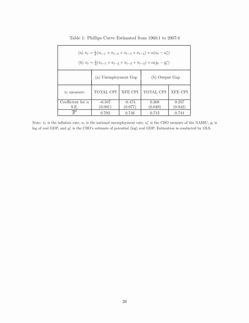
Table 1: Phillips Curve Estimated from 1960:1 to 2007:4
(a) πt =1
4(πt−1 + πt−2 + πt−3 + πt−4) + α(ut − u∗
t)
(b) πt =1
4(πt−1 + πt−2 + πt−3 + πt−4) + α(yt − y∗
t)
(a) Unemployment Gap (b) Output Gap
πt measure: TOTAL CPI XFE CPI TOTAL CPI XFE CPI
Coefficient for α -0.507 -0.474 0.308 0.257S.E. (0.091) (0.077) (0.049) (0.042)
R2
0.703 0.746 0.713 0.744
Note: πt is the inflation rate, ut is the national unemployment rate, u∗
t is the CBO measure of the NAIRU, yt is
log of real GDP, and y∗
t is the CBO’s estimate of potential (log) real GDP. Estimation is conducted by OLS.
38
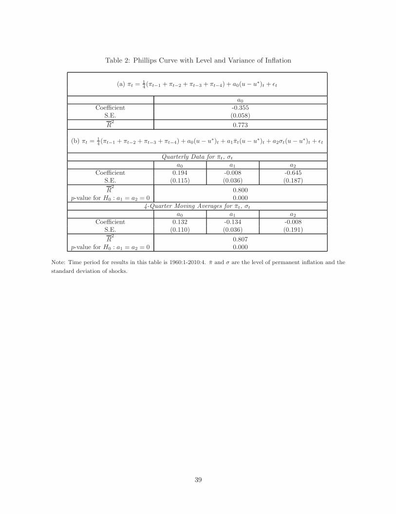
Table 2: Phillips Curve with Level and Variance of Inflation
(a) πt =1
4(πt−1 + πt−2 + πt−3 + πt−4) + a0(u− u∗)t + ǫt
a0Coefficient -0.355
S.E. (0.058)
R2
0.773
(b) πt =1
4(πt−1 + πt−2 + πt−3 + πt−4) + a0(u− u∗)t + a1πt(u− u∗)t + a2σt(u− u∗)t + ǫt
Quarterly Data for πt, σt
a0 a1 a2Coefficient 0.194 -0.008 -0.645
S.E. (0.115) (0.036) (0.187)
R2
0.800p-value for H0 : a1 = a2 = 0 0.000
4-Quarter Moving Averages for πt, σt
a0 a1 a2Coefficient 0.132 -0.134 -0.008
S.E. (0.110) (0.036) (0.191)
R2
0.807p-value for H0 : a1 = a2 = 0 0.000
Note: Time period for results in this table is 1960:1-2010:4. π and σ are the level of permanent inflation and the
standard deviation of shocks.
39
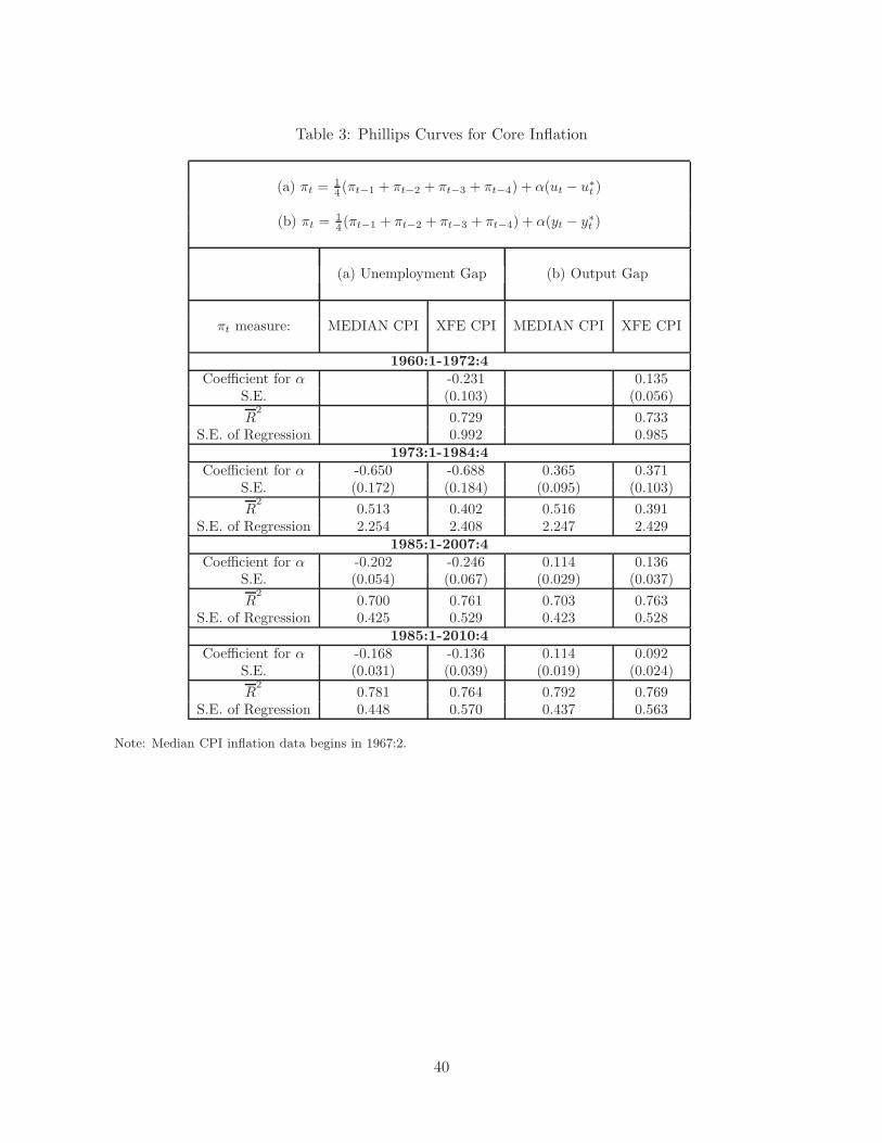
Table 3: Phillips Curves for Core Inflation
(a) πt =1
4(πt−1 + πt−2 + πt−3 + πt−4) + α(ut − u∗
t)
(b) πt =1
4(πt−1 + πt−2 + πt−3 + πt−4) + α(yt − y∗
t)
(a) Unemployment Gap (b) Output Gap
πt measure: MEDIAN CPI XFE CPI MEDIAN CPI XFE CPI
1960:1-1972:4
Coefficient for α -0.231 0.135S.E. (0.103) (0.056)
R2
0.729 0.733S.E. of Regression 0.992 0.985
1973:1-1984:4
Coefficient for α -0.650 -0.688 0.365 0.371S.E. (0.172) (0.184) (0.095) (0.103)
R2
0.513 0.402 0.516 0.391S.E. of Regression 2.254 2.408 2.247 2.429
1985:1-2007:4
Coefficient for α -0.202 -0.246 0.114 0.136S.E. (0.054) (0.067) (0.029) (0.037)
R2
0.700 0.761 0.703 0.763S.E. of Regression 0.425 0.529 0.423 0.528
1985:1-2010:4
Coefficient for α -0.168 -0.136 0.114 0.092S.E. (0.031) (0.039) (0.019) (0.024)
R2
0.781 0.764 0.792 0.769S.E. of Regression 0.448 0.570 0.437 0.563
Note: Median CPI inflation data begins in 1967:2.
40
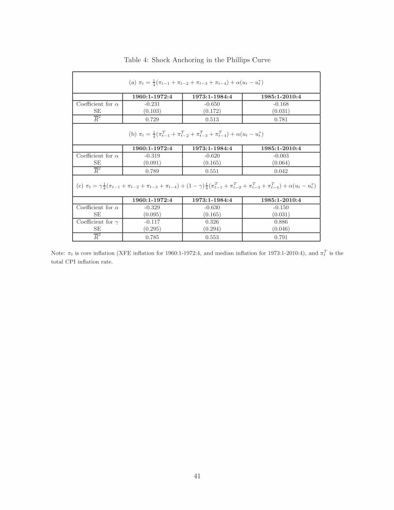
Table 4: Shock Anchoring in the Phillips Curve
(a) πt =14(πt−1 + πt−2 + πt−3 + πt−4) + α(ut − u∗
t )
1960:1-1972:4 1973:1-1984:4 1985:1-2010:4
Coefficient for α -0.231 -0.650 -0.168SE (0.103) (0.172) (0.031)
R2
0.729 0.513 0.781
(b) πt =14(πT
t−1 + πTt−2 + πT
t−3 + πTt−4) + α(ut − u∗
t )
1960:1-1972:4 1973:1-1984:4 1985:1-2010:4
Coefficient for α -0.319 -0.620 -0.003SE (0.091) (0.165) (0.064)
R2
0.789 0.551 0.042
(c) πt = γ 14(πt−1 + πt−2 + πt−3 + πt−4) + (1− γ) 1
4(πT
t−1 + πTt−2 + πT
t−3 + πTt−4) + α(ut − u∗
t )
1960:1-1972:4 1973:1-1984:4 1985:1-2010:4
Coefficient for α -0.329 -0.630 -0.150SE (0.095) (0.165) (0.031)
Coefficient for γ -0.117 0.326 0.886SE (0.295) (0.294) (0.046)
R2
0.785 0.553 0.791
Note: πt is core inflation (XFE inflation for 1960:1-1972:4, and median inflation for 1973:1-2010:4), and πTt is the
total CPI inflation rate.
41
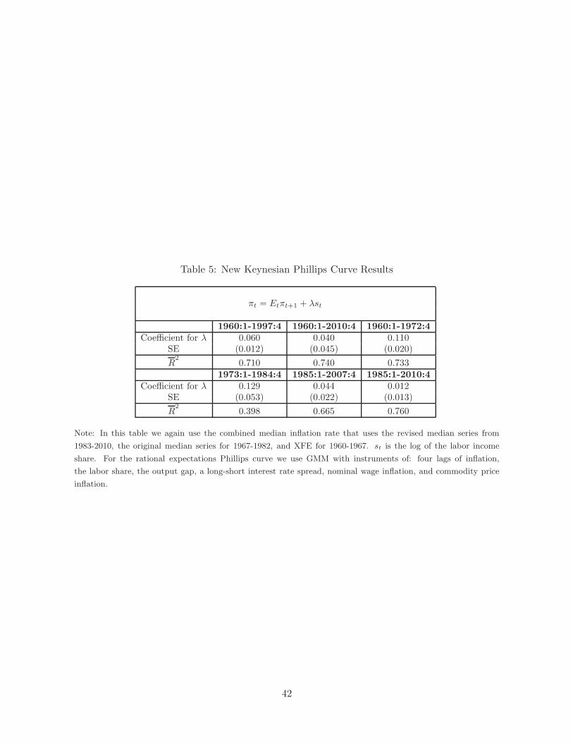
Table 5: New Keynesian Phillips Curve Results
πt = Etπt+1 + λst
1960:1-1997:4 1960:1-2010:4 1960:1-1972:4
Coefficient for λ 0.060 0.040 0.110SE (0.012) (0.045) (0.020)
R2
0.710 0.740 0.7331973:1-1984:4 1985:1-2007:4 1985:1-2010:4
Coefficient for λ 0.129 0.044 0.012SE (0.053) (0.022) (0.013)
R2
0.398 0.665 0.760
Note: In this table we again use the combined median inflation rate that uses the revised median series from
1983-2010, the original median series for 1967-1982, and XFE for 1960-1967. st is the log of the labor income
share. For the rational expectations Phillips curve we use GMM with instruments of: four lags of inflation,
the labor share, the output gap, a long-short interest rate spread, nominal wage inflation, and commodity price
inflation.
42
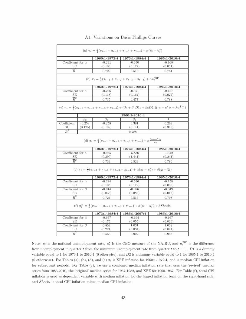
A1. Variations on Basic Phillips Curves
(a) πt =14(πt−1 + πt−2 + πt−3 + πt−4) + α(ut − u∗
t)
1960:1-1972:4 1973:1-1984:4 1985:1-2010:4
Coefficient for α -0.231 -0.650 -0.168SE (0.103) (0.172) (0.031)
R2
0.729 0.513 0.781
(b) πt =14(πt−1 + πt−2 + πt−3 + πt−4) + αuSW
t
1960:1-1972:4 1973:1-1984:4 1985:1-2010:4
Coefficient for α -0.296 -0.521 -0.157SE (0.118) (0.164) (0.027)
R2
0.735 0.477 0.788
(c) πt =14(πt−1 + πt−2 + πt−3 + πt−4) + (β0 + β1D1t + β2D2t)((u − u∗)t + λuSW
t)
1960:1-2010:4
β0 β1 β2 λ
Coefficient -0.259 -0.258 0.381 0.269SE (0.125) (0.189) (0.141) (0.340)
R2
0.788
(d) πt =14(πt−1 + πt−2 + πt−3 + πt−4) + α
(u−u∗)t
ut
1960:1-1972:4 1973:1-1984:4 1985:1-2010:4
Coefficient for α -0.965 -5.836 -1.312SE (0.390) (1.441) (0.241)
R2
0.734 0.529 0.780
(e) πt =14(πt−1 + πt−2 + πt−3 + πt−4) + α(ut − u∗
t) + β(gt − gt)
1960:1-1972:4 1973:1-1984:4 1985:1-2010:4
Coefficient for α -0.224 -0.636 -0.158SE (0.105) (0.172) (0.030)
Coefficient for β -0.014 -0.096 -0.049SE (0.033) (0.085) (0.016)
R2
0.724 0.515 0.798
(f) πTt
= 14(πt−1 + πt−2 + πt−3 + πt−4) + α(ut − u∗
t) + βShockt
1973:1-1984:4 1985:1-2007:4 1985:1-2010:4
Coefficient for α -0.667 -0.194 -0.167SE (0.175) (0.055) (0.030)
Coefficient for β 0.852 1.031 1.038SE (0.221) (0.034) (0.024)
R2
0.566 0.922 0.953
Note: ut is the national unemployment rate, u∗
t is the CBO measure of the NAIRU, and uSWt is the difference
from unemployment in quarter t from the minimum unemployment rate from quarter t to t− 11. D1 is a dummy
variable equal to 1 for 1973:1 to 2010:4 (0 otherwise), and D2 is a dummy variable equal to 1 for 1985:1 to 2010:4
(0 otherwise). For Tables (a), (b), (d), and (e) πt is XFE inflation for 1960:1-1972:4, and is median CPI inflation
for subsequent periods. For Table (c), we use a combined median inflation rate that uses the ‘revised’ median
series from 1983-2010, the ‘original’ median series for 1967-1982, and XFE for 1960-1967. For Table (f), total CPI
inflation is used as dependent variable with median inflation for the lagged inflation term on the right-hand side,
and Shockt is total CPI inflation minus median CPI inflation.
43
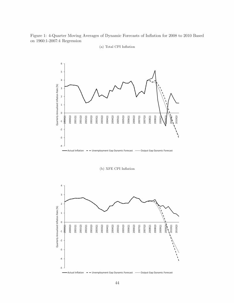
Figure 1: 4-Quarter Moving Averages of Dynamic Forecasts of Inflation for 2008 to 2010 Basedon 1960:1-2007:4 Regression
(a) Total CPI Inflation
5
6
4
(%)
2
3
flation
Rate
(
0
1
Annualized
In
!1
2000Q1
2000Q3
2001Q1
2001Q3
2002Q1
2002Q3
2003Q1
2003Q3
2004Q1
2004Q3
2005Q1
2005Q3
2006Q1
2006Q3
2007Q1
2007Q3
2008Q1
2008Q3
2009Q1
2009Q3
2010Q1
2010Q3
Quarterly A
!3
!2
!4
Actual Inflation Unemployment Gap Dynamic Forecast Output Gap Dynamic Forecast
(b) XFE CPI Inflation
3
4
2
(%)
0
1
flation
Rate
(
!1
0
2000Q1
2000Q3
2001Q1
2001Q3
2002Q1
2002Q3
2003Q1
2003Q3
2004Q1
2004Q3
2005Q1
2005Q3
2006Q1
2006Q3
2007Q1
2007Q3
2008Q1
2008Q3
2009Q1
2009Q3
2010Q1
2010Q3
Annualized
In
3
!2
Quarterly A
!4
!3
!5
Actual Inflation Unemployment Gap Dynamic Forecast Output Gap Dynamic Forecast
44
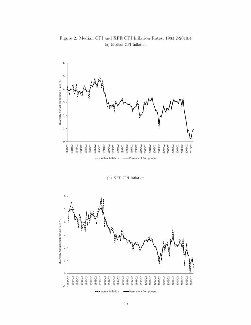
Figure 2: Median CPI and XFE CPI Inflation Rates, 1983:2-2010:4
(a) Median CPI Inflation
6
4
5
Rate
(%)
3
4
ed
Inflation
R
2
erly Annualiz
1
Quarte
0
Q2
Q2
Q2
Q2
Q2
Q2
Q2
Q2
Q2
Q2
Q2
Q2
Q2
Q2
Q2
Q2
Q2
Q2
Q2
Q2
Q2
Q2
Q2
Q2
Q2
Q2
Q2
Q2
1983Q
1984Q
1985Q
1986Q
1987Q
1988Q
1989Q
1990Q
1991Q
1992Q
1993Q
1994Q
1995Q
1996Q
1997Q
1998Q
1999Q
2000Q
2001Q
2002Q
2003Q
2004Q
2005Q
2006Q
2007Q
2008Q
2009Q
2010Q
Actual Inflation Permanent Component
(b) XFE CPI Inflation
6
4
5
(%)
3
4
flation
Rate
(
2
Annualized
In
1
Quarterly A
0
3Q2
4Q2
5Q2
6Q2
7Q2
8Q2
9Q2
0Q2
1Q2
2Q2
3Q2
4Q2
5Q2
6Q2
7Q2
8Q2
9Q2
0Q2
1Q2
2Q2
3Q2
4Q2
5Q2
6Q2
7Q2
8Q2
9Q2
0Q2
!1
1983
1984
1985
1986
1987
1988
1989
1990
1991
1992
1993
1994
1995
1996
1997
1998
1999
2000
2001
2002
2003
2004
2005
2006
2007
2008
2009
2010
Actual Inflation Permanent Component
45
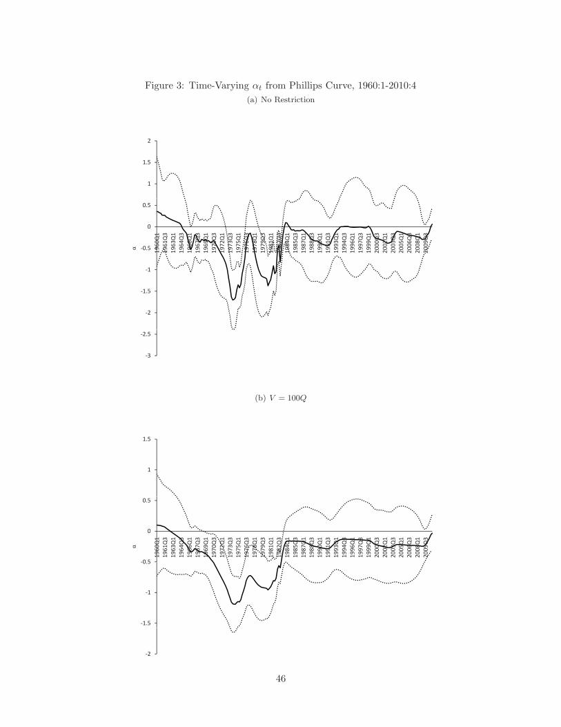
Figure 3: Time-Varying αt from Phillips Curve, 1960:1-2010:4
(a) No Restriction
1.5
2
1
0
0.5
0.5
1960Q1
1961Q3
1963Q1
1964Q3
1966Q1
1967Q3
1969Q1
1970Q3
1972Q1
1973Q3
1975Q1
1976Q3
1978Q1
1979Q3
1981Q1
1982Q3
1984Q1
1985Q3
1987Q1
1988Q3
1990Q1
1991Q3
1993Q1
1994Q3
1996Q1
1997Q3
1999Q1
2000Q3
2002Q1
2003Q3
2005Q1
2006Q3
2008Q1
2009Q3
1.5
1
2
3
2.5
(b) V = 100Q
1.5
1
0
0.5
0 5
0
1960Q1
1961Q3
1963Q1
1964Q3
1966Q1
1967Q3
1969Q1
1970Q3
1972Q1
1973Q3
1975Q1
1976Q3
1978Q1
1979Q3
1981Q1
1982Q3
1984Q1
1985Q3
1987Q1
1988Q3
1990Q1
1991Q3
1993Q1
1994Q3
1996Q1
1997Q3
1999Q1
2000Q3
2002Q1
2003Q3
2005Q1
2006Q3
2008Q1
2009Q3
1
0.5
1.5
2
46
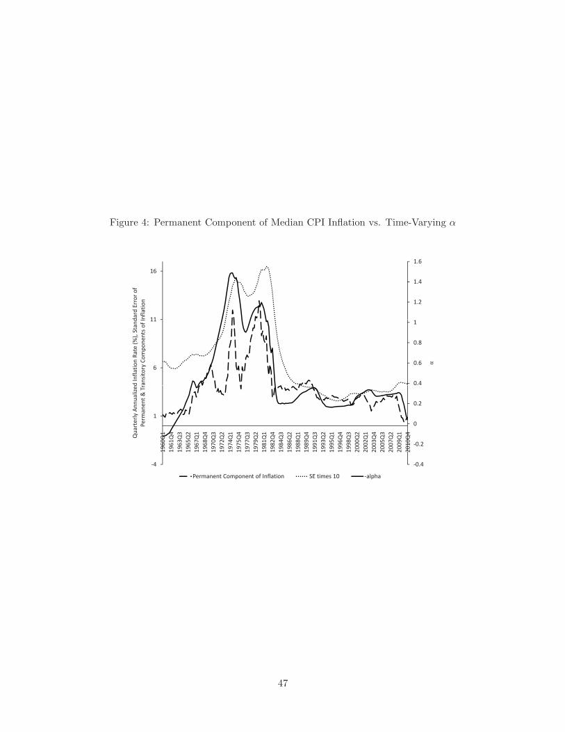
Figure 4: Permanent Component of Median CPI Inflation vs. Time-Varying α
1.4
1.6
16
1.2
11dard
Error of
nflation
0.8
111
ate
(%),
Stand
mponents
of I
0.4
0.66
d Inflation
Ra
ansitory
Com
0.2
1rly Annualized
rmanent &
Tr
!0.2
0
1960Q1
1961Q4
1963Q3
1965Q2
1967Q1
1968Q4
1970Q3
1972Q2
1974Q1
1975Q4
1977Q3
1979Q2
1981Q1
1982Q4
1984Q3
1986Q2
1988Q1
1989Q4
1991Q3
1993Q2
1995Q1
1996Q4
1998Q3
2000Q2
2002Q1
2003Q4
2005Q3
2007Q2
2009Q1
2010Q4
Quarter
Per
!0.4!4
1 1 1 1 1 1 1 1 1 1 1 1 1 1 1 1 1 1 1 1 1 1 1 2 2 2 2 2 2 2
Permanent Component of Inflation SE times 10 !alpha
47
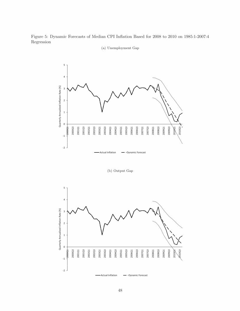
Figure 5: Dynamic Forecasts of Median CPI Inflation Based for 2008 to 2010 on 1985:1-2007:4Regression
(a) Unemployment Gap
5
3
4
(%)
2
3
flation
Rate
(
1
Annualized
In
0
Q1
Q3
Q1
Q3
Q1
Q3
Q1
Q3
Q1
Q3
Q1
Q3
Q1
Q3
Q1
Q3
Q1
Q3
Q1
Q3
Q1
Q3Quarterly A
!1
2000Q
2000Q
2001Q
2001Q
2002Q
2002Q
2003Q
2003Q
2004Q
2004Q
2005Q
2005Q
2006Q
2006Q
2007Q
2007Q
2008Q
2008Q
2009Q
2009Q
2010Q
2010Q
!2
Actual Inflation Dynamic Forecast
(b) Output Gap
5
3
4
(%)
2
3
flation
Rate
(
1
Annualized
In
0
Q1
Q3
Q1
Q3
Q1
Q3
Q1
Q3
Q1
Q3
Q1
Q3
Q1
Q3
Q1
Q3
Q1
Q3
Q1
Q3
Q1
Q3Quarterly A
!1
2000Q
2000Q
2001Q
2001Q
2002Q
2002Q
2003Q
2003Q
2004Q
2004Q
2005Q
2005Q
2006Q
2006Q
2007Q
2007Q
2008Q
2008Q
2009Q
2009Q
2010Q
2010Q
!2
Actual Inflation Dynamic Forecast
48
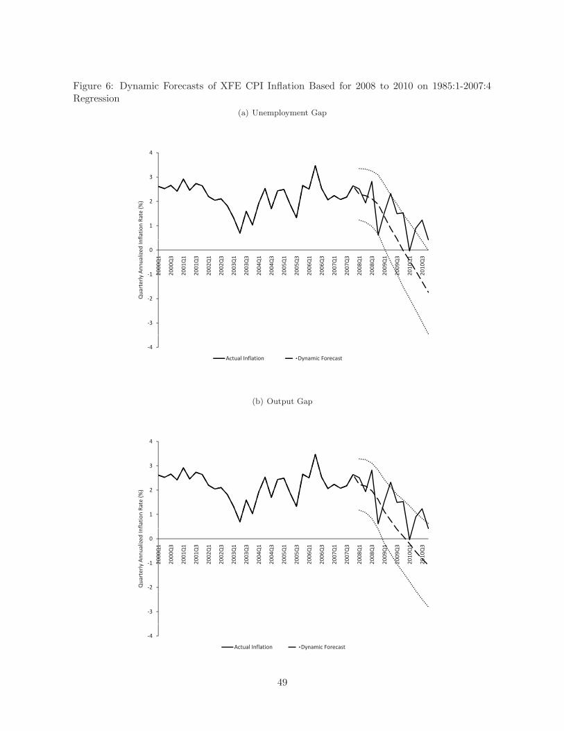
Figure 6: Dynamic Forecasts of XFE CPI Inflation Based for 2008 to 2010 on 1985:1-2007:4Regression
(a) Unemployment Gap
3
4
2
3
(%)
1
flation
Rate
(
0
000Q1
000Q3
001Q1
001Q3
002Q1
002Q3
003Q1
003Q3
004Q1
004Q3
005Q1
005Q3
006Q1
006Q3
007Q1
007Q3
008Q1
008Q3
009Q1
009Q3
010Q1
010Q3
Annualized
In
!2
!1 20
20
20
20
20
20
20
20
20
20
20
20
20
20
20
20
20
20
20
20
20
20
Quarterly A
!3
!4
Actual Inflation Dynamic Forecast
(b) Output Gap
3
4
2
3
(%)
1
flation
Rate
(
0
000Q1
000Q3
001Q1
001Q3
002Q1
002Q3
003Q1
003Q3
004Q1
004Q3
005Q1
005Q3
006Q1
006Q3
007Q1
007Q3
008Q1
008Q3
009Q1
009Q3
010Q1
010Q3
Annualized
In
!2
!1 20
20
20
20
20
20
20
20
20
20
20
20
20
20
20
20
20
20
20
20
20
20
Quarterly A
!3
!4
Actual Inflation Dynamic Forecast
49
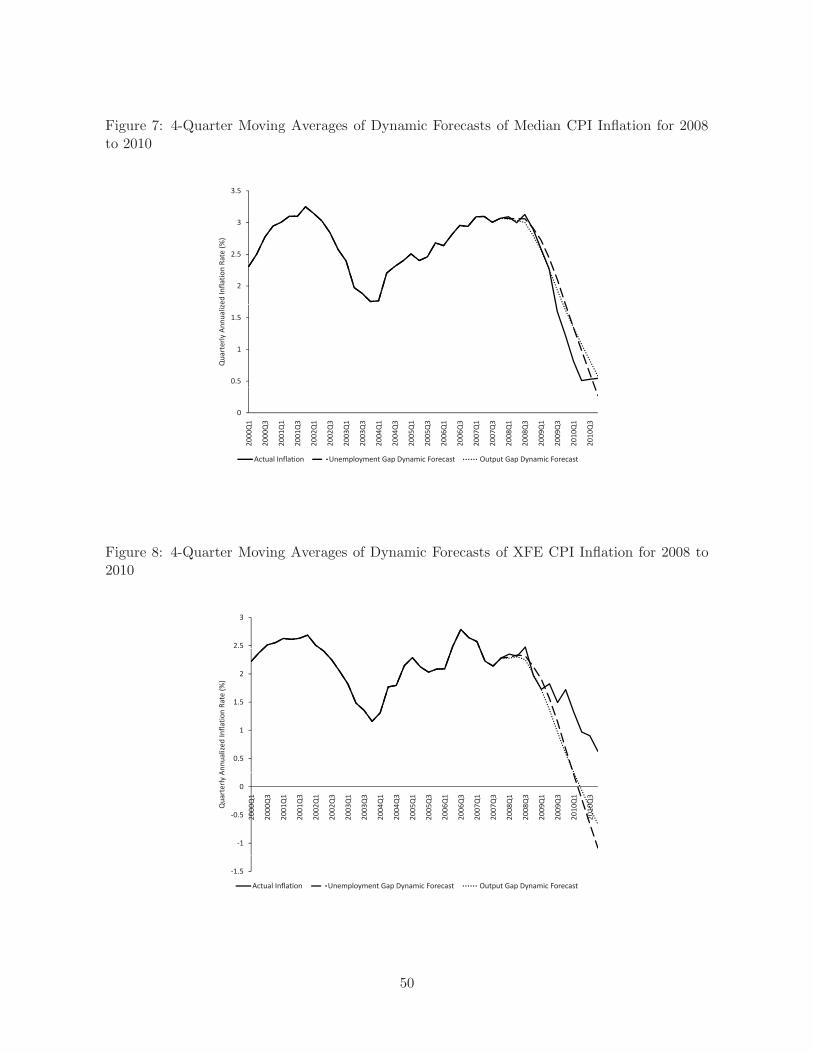
Figure 7: 4-Quarter Moving Averages of Dynamic Forecasts of Median CPI Inflation for 2008to 2010
3
3.5
2.5
3Rate
(%)
2
ed
Inflation
R
1.5
erly Annualiz
0.5
1
Quarte
0
Q1
Q3
Q1
Q3
Q1
Q3
Q1
Q3
Q1
Q3
Q1
Q3
Q1
Q3
Q1
Q3
Q1
Q3
Q1
Q3
Q1
Q3
2000Q
2000Q
2001Q
2001Q
2002Q
2002Q
2003Q
2003Q
2004Q
2004Q
2005Q
2005Q
2006Q
2006Q
2007Q
2007Q
2008Q
2008Q
2009Q
2009Q
2010Q
2010Q
Actual Inflation Unemployment Gap Dynamic Forecast Output Gap Dynamic Forecast
Figure 8: 4-Quarter Moving Averages of Dynamic Forecasts of XFE CPI Inflation for 2008 to2010
2.5
3
2
(%)
1
1.5
flation
Rate
(
0.5
1
Annualized
In
0 5
0
000Q1
000Q3
001Q1
001Q3
002Q1
002Q3
003Q1
003Q3
004Q1
004Q3
005Q1
005Q3
006Q1
006Q3
007Q1
007Q3
008Q1
008Q3
009Q1
009Q3
010Q1
010Q3
Quarterly A
!1
!0.5 20
20
20
20
20
20
20
20
20
20
20
20
20
20
20
20
20
20
20
20
20
20
!1.5
Actual Inflation Unemployment Gap Dynamic Forecast Output Gap Dynamic Forecast
50
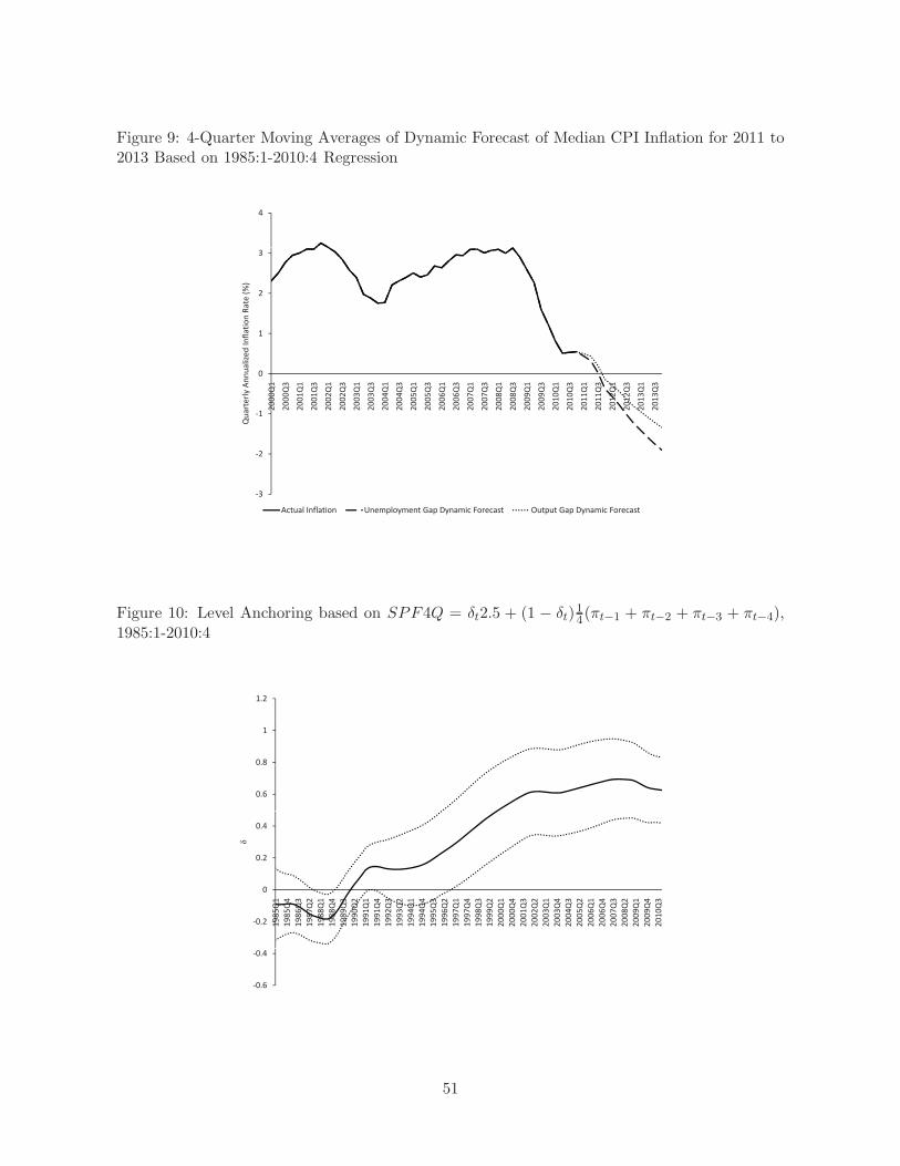
Figure 9: 4-Quarter Moving Averages of Dynamic Forecast of Median CPI Inflation for 2011 to2013 Based on 1985:1-2010:4 Regression
4
2
3(%
)
1
2
flation
Rate
(
0
1 3 1 3 1 3 1 3 1 3 1 3 1 3 1 3 1 3 1 3 1 3 1 3 1 3 1 3Annualized
In
!1
2000Q1
2000Q3
2001Q1
2001Q3
2002Q1
2002Q3
2003Q1
2003Q3
2004Q1
2004Q3
2005Q1
2005Q3
2006Q1
2006Q3
2007Q1
2007Q3
2008Q1
2008Q3
2009Q1
2009Q3
2010Q1
2010Q3
2011Q1
2011Q3
2012Q1
2012Q3
2013Q1
2013Q3
Quarterly A
!2
!3
Actual Inflation Unemployment Gap Dynamic Forecast Output Gap Dynamic Forecast
Figure 10: Level Anchoring based on SPF4Q = δt2.5 + (1 − δt)14(πt−1 + πt−2 + πt−3 + πt−4),
1985:1-2010:4
1.2
0.8
1
0.6
0 2
0.4
0
0.2
Q1
Q4
Q3
Q2
Q1
Q4
Q3
Q2
Q1
Q4
Q3
Q2
Q1
Q4
Q3
Q2
Q1
Q4
Q3
Q2
Q1
Q4
Q3
Q2
Q1
Q4
Q3
Q2
Q1
Q4
Q3
Q2
Q1
Q4
Q3
0.2 1985Q
1985Q
1986Q
1987Q
1988Q
1988Q
1989Q
1990Q
1991Q
1991Q
1992Q
1993Q
1994Q
1994Q
1995Q
1996Q
1997Q
1997Q
1998Q
1999Q
2000Q
2000Q
2001Q
2002Q
2003Q
2003Q
2004Q
2005Q
2006Q
2006Q
2007Q
2008Q
2009Q
2009Q
2010Q
0.6
0.4
51
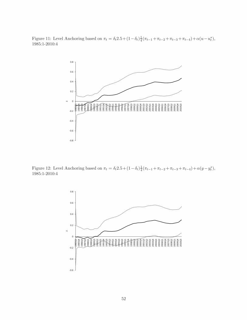
Figure 11: Level Anchoring based on πt = δt2.5+(1−δt)14(πt−1+πt−2+πt−3+πt−4)+α(u−u∗t ),
1985:1-2010:4
0.8
0.6
0.2
0.4
0
Q1
Q4
Q3
Q2
Q1
Q4
Q3
Q2
Q1
Q4
Q3
Q2
Q1
Q4
Q3
Q2
Q1
Q4
Q3
Q2
Q1
Q4
Q3
Q2
Q1
Q4
Q3
Q2
Q1
Q4
Q3
Q2
Q1
Q4
Q3
0.2 1985Q
1985Q
1986Q
1987Q
1988Q
1988Q
1989Q
1990Q
1991Q
1991Q
1992Q
1993Q
1994Q
1994Q
1995Q
1996Q
1997Q
1997Q
1998Q
1999Q
2000Q
2000Q
2001Q
2002Q
2003Q
2003Q
2004Q
2005Q
2006Q
2006Q
2007Q
2008Q
2009Q
2009Q
2010Q
0 6
0.4
0.8
0.6
Figure 12: Level Anchoring based on πt = δt2.5+(1−δt)14 (πt−1+πt−2+πt−3+πt−4)+α(y−y∗t ),
1985:1-2010:4
0.8
0.6
0.4
0.2
0 2
0
1985Q1
1985Q4
1986Q3
1987Q2
1988Q1
1988Q4
1989Q3
1990Q2
1991Q1
1991Q4
1992Q3
1993Q2
1994Q1
1994Q4
1995Q3
1996Q2
1997Q1
1997Q4
1998Q3
1999Q2
2000Q1
2000Q4
2001Q3
2002Q2
2003Q1
2003Q4
2004Q3
2005Q2
2006Q1
2006Q4
2007Q3
2008Q2
2009Q1
2009Q4
2010Q3
0.4
0.2
0.6
52
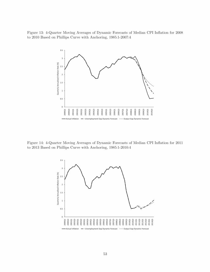
Figure 13: 4-Quarter Moving Averages of Dynamic Forecasts of Median CPI Inflation for 2008to 2010 Based on Phillips Curve with Anchoring, 1985:1-2007:4
3
3.5
2.5
3Rate
(%)
2
ed
Inflation
R
1.5
erly Annualize
0.5
1
Quarte
0
Q1
Q3
Q1
Q3
Q1
Q3
Q1
Q3
Q1
Q3
Q1
Q3
Q1
Q3
Q1
Q3
Q1
Q3
Q1
Q3
Q1
Q3
2000Q
2000Q
2001Q
2001Q
2002Q
2002Q
2003Q
2003Q
2004Q
2004Q
2005Q
2005Q
2006Q
2006Q
2007Q
2007Q
2008Q
2008Q
2009Q
2009Q
2010Q
2010Q
Actual Inflation Unemployment Gap Dynamic Forecast Output Gap Dynamic Forecast
Figure 14: 4-Quarter Moving Averages of Dynamic Forecasts of Median CPI Inflation for 2011to 2013 Based on Phillips Curve with Anchoring, 1985:1-2010:4
3
3.5
2.5
3
Rate
(%)
2
ed
Inflation
R
1.5
erly Annualiz
0.5
1
Quarte
0
Q1
Q3
Q1
Q3
Q1
Q3
Q1
Q3
Q1
Q3
Q1
Q3
Q1
Q3
Q1
Q3
Q1
Q3
Q1
Q3
Q1
Q3
Q1
Q3
Q1
Q3
Q1
Q3
2000Q
2000Q
2001Q
2001Q
2002Q
2002Q
2003Q
2003Q
2004Q
2004Q
2005Q
2005Q
2006Q
2006Q
2007Q
2007Q
2008Q
2008Q
2009Q
2009Q
2010Q
2010Q
2011Q
2011Q
2012Q
2012Q
2013Q
2013Q
Actual Inflation Unemployment Gap Dynamic Forecast Output Gap Dynamic Forecast
53
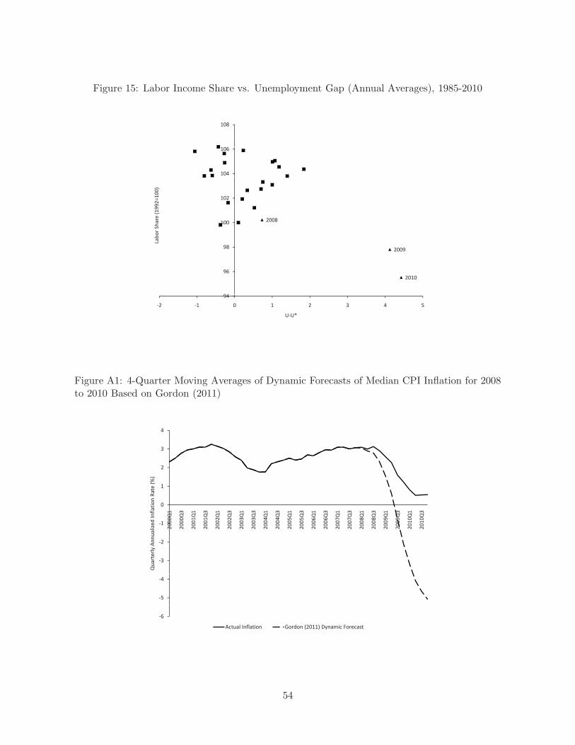
Figure 15: Labor Income Share vs. Unemployment Gap (Annual Averages), 1985-2010
108
104
106
102
92=100)
2008100
bor Share
(199
200998
Lab
2010
94
96
94
!2 !1 0 1 2 3 4 5
U!U*
Figure A1: 4-Quarter Moving Averages of Dynamic Forecasts of Median CPI Inflation for 2008to 2010 Based on Gordon (2011)
3
4
2
(%)
0
1
Q1
Q3
Q1
Q3
Q1
Q3
Q1
Q3
Q1
Q3
Q1
Q3
Q1
Q3
Q1
Q3
Q1
Q3
Q1
Q3
Q1
Q3flation
Rate
(
!2
!1
2000Q
2000Q
2001Q
2001Q
2002Q
2002Q
2003Q
2003Q
2004Q
2004Q
2005Q
2005Q
2006Q
2006Q
2007Q
2007Q
2008Q
2008Q
2009Q
2009Q
2010Q
2010Q
Annualized
In
!3
Quarterly A
!5
!4
!6
Actual Inflation Gordon (2011) Dynamic Forecast
54