NBER WORKING PAPER SERIES

INFLATION-GAP PERSISTENCE IN THE U.S.

Timothy CogleyGiorgio E. PrimiceriThomas J. Sargent

Working Paper 13749http://www.nber.org/papers/w13749

NATIONAL BUREAU OF ECONOMIC RESEARCH1050 Massachusetts Avenue

Cambridge, MA 02138January 2008

For comments and suggestions, we thank James Kahn, Spencer Krane, and seminar participants atthe Federal Reserve Board, the Federal Reserve Bank of Chicago, the Summer 2007 meetings of theSociety for Computational Economics, and the EABCN Workshop on "Changes in Inflation Dynamicsand Implications for Forecasting."We are also grateful to Francisco Barillas and Christian Matthesfor research assistance. Sargent thanks the National Science Foundation for research support througha grant to the National Bureau of Economic Research. The views expressed herein are those of theauthor(s) and do not necessarily reflect the views of the National Bureau of Economic Research.

NBER working papers are circulated for discussion and comment purposes. They have not been peer-reviewed or been subject to the review by the NBER Board of Directors that accompanies officialNBER publications.

© 2008 by Timothy Cogley, Giorgio E. Primiceri, and Thomas J. Sargent. All rights reserved. Shortsections of text, not to exceed two paragraphs, may be quoted without explicit permission providedthat full credit, including © notice, is given to the source.

Inflation-Gap Persistence in the U.S.Timothy Cogley, Giorgio E. Primiceri, and Thomas J. SargentNBER Working Paper No. 13749January 2008JEL No. C11,C15,C32,E3,E52

ABSTRACT

We use Bayesian methods to estimate two models of post WWII U.S. inflation rates with drifting stochasticvolatility and drifting coefficients. One model is univariate, the other a multivariate autoregression.We define the inflation gap as the deviation of inflation from a pure random walk component of inflationand use both of our models to study changes over time in the persistence of the inflation gap measuredin terms of short- to medium-term predicability. We present evidence that our measure of the inflation-gappersistence increased until Volcker brought mean inflation down in the early 1980s and that it thenfell during the chairmanships of Volcker and Greenspan. Stronger evidence for movements in inflationgap persistence emerges from the VAR than from the univariate model. We interpret these changesin terms of a simple dynamic new Keynesian model that allows us to distinguish altered monetarypolicy rules and altered private sector parameters.

Timothy CogleyUniversity of California, DavisEconomics DepartmentOne Shields Ave.Davis, CA 95616twcogley@ucdavis.edu

Giorgio E. PrimiceriNorthwestern UniversityDepartment of Economics2001 Sheridan Road3218 Andersen HallEvanston, Il. 60208-2600and NBERg-primiceri@northwestern.edu

Thomas J. SargentDepartment of EconomicsNew York University19 W. 4th Street, 6th FloorNew York, NY 10012and NBERthomas.sargent@nyu.edu

Inflation-Gap Persistence in the U.S.∗

Timothy Cogley,† Giorgio E. Primiceri,‡ and Thomas J. Sargent§

Revised: December 2007

Abstract

We use Bayesian methods to estimate two models of post WWII U.S. in-flation rates with drifting stochastic volatility and drifting coefficients. Onemodel is univariate, the other a multivariate autoregression. We define theinflation gap as the deviation of inflation from a pure random walk componentof inflation and use both models to study changes over time in the persistenceof the inflation gap measured in terms of short- to medium-term predicability.We present evidence that our measure of the inflation-gap persistence increaseduntil Volcker brought mean inflation down in the early 1980s and that it thenfell during the chairmanships of Volcker and Greenspan. Stronger evidence formovements in inflation gap persistence emerges from the VAR than from theunivariate model. We interpret these changes in terms of a simple dynamicnew Keynesian model that allows us to distinguish altered monetary policyrules and altered private sector parameters.

1 Introduction

This paper studies how inflation persistence has changed since the Great Inflation.We distinguish the persistence of inflation from the persistence of a component of itcalled the inflation gap. Our first message is that although inflation remains highlypersistent, the inflation gap became less persistent after the Volcker disinflation. Oursecond message is that multivariate information helps to detect changes in inflation-gap persistence. Although the univariate evidence is mixed, a clearer picture emerges

∗For comments and suggestions, we thank James Kahn, Spencer Krane, and seminar participantsat the Federal Reserve Board, the Federal Reserve Bank of Chicago, the Summer 2007 meetings ofthe Society for Computational Economics, and the EABCN Workshop on “Changes in InflationDynamics and Implications for Forecasting.”We are also grateful to Francisco Barillas and Chris-tian Matthes for research assistance. Sargent thanks the National Science Foundation for researchsupport through a grant to the National Bureau of Economic Research.

†University of California, Davis. Email: twcogley@ucdavis.edu.‡Northwestern University. Email: g-primiceri@northwestern.edu.§New York University and Hoover Institution, Stanford University. Email: ts43@nyu.edu.

1

from a VAR. Our third message is that the decline in inflation-gap persistence seemsto be due for the most part to lower variability of changes in the Fed’s long-runinflation target.

We decompose inflation into two parts, a stochastic trend τt that (to a first-orderapproximation) evolves as a driftless random walk, and an inflation gap gt = πt − τt

that represents temporary differences between actual and trend inflation. In generalequilibrium models, trend inflation is usually pinned down by a central bank’s target,a view that associates movements in trend inflation with shifts in the Federal Reserve’starget. Because trend inflation is a driftless random walk, actual inflation has a unitautoregressive root and is highly persistent. In our view, target inflation has notstopped drifting, though its conditional variance has declined.1

Transient movements in the inflation gap are layered on top of τt. (Cogley andSargent 2001 and 2005a) reported weak evidence of a decline in inflation-gap persis-tence. Several authors have challenged the statistical significance of that evidence(e.g., see Sims 2001, Stock 2001, and Pivetta and Reis 2007). Here we report newevidence that is more decisive. We can now say that it is very likely that inflation-gappersistence has decreased since the Great Inflation.

We organize the discussion as follows. We begin with an unobserved componentsmodel of Stock and Watson (2007) and relate it to the drifting-parameter VARs ofCogley and Sargent (2005a) and Primiceri (2005). We use these statistical models todefine trend inflation and to focus attention on the inflation gap.

Next we define a measure of persistence in terms of the predictability of theinflation gap,2 in particular, as the fraction of total inflation-gap variation j quartersahead that is due to shocks inherited from the past. We say that the inflation gapis weakly persistent when the effects of shocks decay quickly and that it is stronglypersistent when they decay slowly. When the effects of past shocks die out quickly,future shocks account for most of the variation in gt+j, pushing our measure close tozero. But when the effects of past shocks on gt+j decay slowly, they account for ahigher proportion of near-term movements, pushing our measure of persistence closerto one. Thus, a large fraction of variation over short to medium horizons that isdue to past shocks signifies strong persistence and a small fraction indicates weakpersistence.

Under a convenient approximation, our measure is the R2 statistic for j-stepahead inflation-gap forecasts.3 Heuristically, a connection between predictability and

1For evidence that the innovation variance for τt has declined, see Stock and Watson (2007).2This measure is inspired by Diebold and Kilian (2001). Barsky (1987) used a closely-related

measure to compare inflation persistence under the Gold Standard and after World War II.3Strictly speaking, we should say ‘pseudo forecasts’ because we neglect complications associated

with real-time forecasting. This is not a shortcut; it is intentional. Our goal is to make retrospectivestatements about inflation persistence. To attain as much precision as possible, we use ex postrevised data and estimate parameters using data through the end of the sample.

2

persistence arises because past shocks give rise to forecastable movements in gt+j,

while future shocks contribute to the forecast error. Hence, the continuing influenceof past shocks can be measured by the proportion of predictable variation in gt+j.

We deduce persistence measures from the posterior distribution of a drifting-parameter VAR, then study how they have changed since the Great Inflation. A keyfinding is that inflation gaps were highly predictable circa 1980, but are much less sonow. Furthermore, the evidence of declining persistence is statistically significant atconventional levels. Thus, the statistical results strengthen our conviction that theinflation gap has become less persistent.

Finally, we use a simple dynamic new Keynesian model to examine what causedthe change in the law of motion for inflation. In our DSGE model, improved monetarypolicy is the single most important factor explaining the decline in inflation volatilityand persistence. A key dimension is the reduction in the rate at which the Fed’s targetdrifts. Nevertheless, nonpolicy factors are also important; in particular, we find thatmark-up shocks have become less volatile and persistent, and this also contributesto better inflation outcomes. In our model, better policy and changes in the privatesector both play a role.

2 Unobserved components models for inflation

Stock and Watson (2007) estimate a univariate unobserved components model forinflation. They assume that inflation πt is the sum of a stochastic trend τt and amartingale-difference innovation επt,

πt = τt + επt. (1)

The trend component evolves as a driftless random walk,

τt = τt−1 + ετt. (2)

Equation (1) is the measurement equation for a state-space representation, and equa-tion (2) is the state equation. The innovations επt and ετt are assumed to be martin-gale differences that are conditionally normal with variances hπt and hτt, respectively.The latter are independent stochastic volatilities that evolve as geometric randomwalks,

ln hπt = ln hπt−1 + σπηπt, (3)

ln hτt = ln hτt−1 + στητt

where ηπt and ητt are i.i.d. Gaussian shocks with means of zero that are mutuallyindependent.

3

A consensus has emerged that trend inflation is well approximated by a driftlessrandom walk. Authors who model trend inflation in this way include Cogley andSargent (2001, 2005a), Ireland (2007), Smets and Wouters (2003), and Cogley andSbordone (2006). There is little controversy about this feature of the data. Our mainfocus, however, is on the inflation gap, gt ≡ πt − τt. We want to know how persistentgt is and whether the degree of persistence in gt has changed over time. Stock andWatson’s (2007) model is not a suitable vehicle for investigating this issue because itimposes that gt ≡ επt is serially uncorrelated for all t.

Reading the literature on inflation persistence can be confusing because authorssometimes fail to state clearly what feature of the data they are trying to measure.For instance, Pivetta and Reis (2007) look for changes in inflation persistence byrunning rolling unit-root tests on πt. They find that the largest autoregressive rootis always close to 1 and conclude that inflation persistence is unchanged. But thatfinding can be viewed simply as a manifestation of shifts in target inflation: πt has aunit root because τt drifts. Estimates of the largest autoregressive root in πt wouldhelp measure inflation-gap persistence only if trend inflation were constant over time,an assumption that much of the recent literature denies.4

Stock and Watson’s specification is a useful starting point because it highlightsthe role of τt. But it is not a good vehicle for pursuing questions about inflation-gappersistence because it assumes that gt = επt is a martingale difference. To address thequestions about the persistence of gt that interest us, we must modify their model.

Cogley and Sargent (2005a) estimate a closely related time-varying parameterVAR. Evidence reported there suggests that gt is autocorrelated and that the degreeof serial dependence has probably changed over time. But that model assumed nostochastic volatility in the parameter innovations, a feature that Stock and Watsonsay is important. In this paper, we combine and extend features of Stock and Watson’smodel and our earlier ones to create a new model that lets us focus on the persistenceof the inflation gap.

2.1 A univariate autoregression with drifting parameters

As a first step, we introduce an autoregressive term into Stock and Watson’srepresentation. With this addition, the measurement and state equations become

πt = µt−1 + ρt−1πt−1 + επt, (4)

γt = γt−1 + εst, (5)

where γt = [µt, ρt]′ and εst = [εµt, ερt]

′. Here the vector εst is the noise in a state vector,whose components are parameter values in the measurement equation (4). Notice that

4Levin and Piger (2004) pointed out this shortcoming of Pivetta and Reis. After allowing for ashift in trend inflation, Levin and Piger were able to detect a decline in inflation-gap persistence.

4

the constant term in the measurement equation has become an intercept rather thana local approximation to the mean.5 As in our earlier work, we approximate trendinflation by τt

.= µt/(1 − ρt). To a first-order approximation, this is also a driftless

random walk.6

Equations (4) and (5) describe a univariate autoregression with drifting param-eters. If the innovation variances were all constant, (4)–(5) would be a special caseof the time-varying parameter model of Cogley and Sargent (2001). In Cogley andSargent (2005a) and Primiceri (2005), the measurement-innovation variance is time-varying, but the variance of the state-innovation εst variance is constant. In contrast,Stock and Watson assume that both innovation variances are time varying. Herewe follow Stock and Watson by modeling both innovation variances as stochasticvolatility processes.

We retain Stock and Watson’s specification for var(επt), and we adopt a bivariatestochastic volatility model for the state innovations εst:

var(εst) = Qt = B−1HstB−1′. (6)

As in our earlier work, we assume that Hst is diagonal and that B is lower triangular,

Hst =

(hµt 00 hρt

), (7)

B =

(1 0

β21 1

). (8)

The diagonal elements of Hst are independent, univariate stochastic volatilities thatevolve as driftless, geometric random walks:

ln hit = ln hit−1 + σiηit, (9)

i = π, s. The volatility innovations ηit are mutually independent, standard normalvariates. The variance of ∆ ln hit depends on the free parameter σi. For tractabilityand parsimony, we also assume that εst is uncorrelated at all leads and lags with επt

and that the standardized state and measurement innovations are independent of thevolatility innovations ηt.

This is a convenient specification for modeling recurrent persistent changes invariance. It ensures that Qt is positive definite and allows for time-varying correlationsamong the elements of εst.

We constrain ρt to be less than one in absolute value at all dates. Having assumedthat trend inflation is a driftless random walk, the stability constraint on ρt just rules

5We also adopt a slightly different dating convention. The reason for this dating convention willbecome clear when we discuss predictability. Nothing of substance hinges on this convention.

6A first-order Taylor approximation makes τt a linear function of γt, which evolves as a driftlessrandom walk.

5

out a second unit or explosive root in inflation. There is an emerging consensus thatthe price level is best modeled as an I(2) process, but few economists think that it isI(3). The stability constraint just rules out an I(3) representation.

The model is estimated by Bayesian methods using a Markov Chain Monte Carloalgorithm outlined in appendix A.

2.2 A vector autoregression with drifting parameters

Although a univariate autoregression is a useful first step, it is not entirely satis-factory for representing changes in the inflation process. Cogley and Sargent (2001and 2005a) found evidence of changes in the autocorrelations of the inflation gap andalso in cross-correlations with lags of other variables. Accordingly, we also consider avector autoregression with drifting parameters. Since our definition of the persistenceof gt is based on its predictability, it is interesting to check how findings depend onthe information that we use to condition predictions.

As in Cogley and Sargent (2005a), we estimate a trivariate VAR for inflation,unemployment, and a short-term nominal interest rate. The state and measurementequations for the VAR are

yt = X ′t−1θt−1 + εyt, (10)

θt = θt−1 + εst. (11)

The vector yt contains current observations on the variables of interest, Xt−1 includesconstants plus lags of yt, and εyt is a vector of innovations. The parameter vector θt

evolves as a driftless random walk subject to a reflecting barrier that guarantees thatthe VAR has nonexplosive roots at every date.

We assume that the innovation variances follow multivariate stochastic volatilityprocesses. The state innovation variance Qt has the same form as in the AR(1)model, but has a higher dimension to conform to the size of θt. We assume that themeasurement innovation variance Vt also has this form, again adapting its dimensionsto the size of εyt.

This model is very much like those in Cogley and Sargent (2005a) and Primiceri(2005). The main difference concerns the specification for var(εst). Our earlier pa-pers assumed that the parameter innovation variance was constant; here we adopt astochastic volatility model so that the variance is time varying. Equations (10) and(11) can also be regarded as a multivariate extension of Stock and Watson (2007).We think this model is a useful vehicle for connecting their paper to this one.

We estimate the multivariate model by a Bayesian Markov Chain Monte Carloalgorithm. Details are given in appendix A.1.

In what follows, we make frequent use of the companion form of the VAR,

zt+1 = µt + Atzt + εzt+1. (12)

6

The vector zt includes current and lagged values of yt, the vector µt contains the VARintercepts, and the companion matrix At contains the autoregressive parameters. Weuse the companion form for multi-step forecasting. When we do that, we approximatemulti-step forecasts by assuming that VAR parameters will remain constant at theircurrent values going forward in time. This approximation is common in the literatureon bounded rationality and learning, being a key element of an ‘anticipated-utility’model (Kreps 1998). In other papers, we have found that it does a good job ofapproximating the mean of Bayesian predictive densities (e.g., see Cogley, Morozov,and Sargent 2005 and Cogley and Sargent 2006).

With this assumption, we can form local-to-date t approximations to the momentsof zt. For the unconditional mean, we follow Beveridge and Nelson (1981) by definingthe stochastic trend in zt as the value to which the series is expected to converge inthe long run:

zt = limh→∞

Etzt+h. (13)

With θt held constant at its current value, we approximate this as

zt∼= (I − At)

−1µt. (14)

To a first-order approximation, zt evolves as a driftless random walk, implying thatinflation and the other variables in yt have a unit root. As in the AR(1) model, thestability constraint on At just rules out an I(2) representation for yt.

After subtracting zt from both sides of (12) and invoking the anticipated-utilityapproximation, we get a forecasting model for gap variables,

(zt+1 − zt) = At(zt − zt) + εz,t+1. (15)

We approximate forecasts of gap variables j periods ahead as Ajt zt,

7 and we approx-imate the forecast-error variance by

vart(zt+j) ∼=∑j−1

h=0(Ah

t )var(εz,t+1)(Aht )′. (16)

To approximate the unconditional variance of zt+1, we take the limit of the conditionalvariance as the forecast horizon j increases,8

var(zt+1) ∼=∑∞

h=0(Ah

t )var(εz,t+1)(Aht )′. (17)

Under the anticipated-utility approximation, this is also the unconditional varianceof zt+s for s > 1.

7By the anticipated-utility approximation, Etzt+j = zt. This is a good approximation because zt

is a driftless random walk to a first-order approximation.8This is a second-moment analog to the Beveridge-Nelson trend.

7

3 Persistence and predictability

Let πt = eπzt, where eπ is a selector vector. To measure persistence at a given datet, we calculate the fraction of the total variation in gt+j that is due to shocks inheritedfrom the past relative to those that will occur in the future. This is equivalent to 1minus the fraction of the total variation due to future shocks. Since future shocksaccount for the forecast error, that fraction can be expressed as the ratio of theconditional variance to the unconditional variance,

R2jt = 1− vart(eπzt+j)

var(eπzt+j), (18)

∼= 1−eπ

[∑j−1h=0(A

ht )var(εzt+1)(A

ht )′]e′π

eπ

[∑∞h=0(A

ht )var(εzt+1)(Ah

t )′] e′π

.

We label this R2jt because it is analogous to the R2 statistic for j-step ahead forecasts.

This fraction must lie between zero and one, and it converges to zero as the forecasthorizon j lengthens.9 Whether it converges rapidly or slowly reflects the degree ofpersistence. If past shocks die out quickly, the fraction converges rapidly to zero. Butif one or more shocks decay slowly, the fraction may converge only gradually to zero,possibly remaining close to one for some time. Thus, for small or medium j ≥ 1, asmall fraction signifies weak persistence and a large fraction strong persistence.

In a univariate AR(1) model, things simplify because R2jt depends on a single pa-

rameter ρt. In this case, the unconditional variance is σ2εt/(1−ρ2

t ), and the conditionalvariance is (1− ρ2j

t )σ2εt/(1− ρ2

t ). Therefore, R2jt simplifies to ρ2j

t .

Matters are more complicated if we increase the number of lags or add othervariables. For a VAR, the ratio depends on all of the parameters of the companionmatrix At. Sometimes economists summarize persistence in a VAR by focusing onthe largest autoregressive root in At. This is problematic for at least two reasons.One is that the largest root could be associated not with inflation but with anothervariable in the VAR. Hence the largest root of At might exaggerate persistence inthe inflation gap. Another problem is that two large roots could matter for inflation,in which case the largest root of At would understate the degree of persistence. Wethink it is important to retain all the information in At.

3.1 A caveat

Nevertheless, (18) is not entirely satisfactory because it depends on the conditionalvariance Vt+1 in addition to the conditional mean parameters At. Changes in Vt+1

that take the form of a scalar multiplication are not a problem because the scalarwould cancel in numerator and denominator. But R2

jt is not invariant to other changes

9This follows from the stability constraint on At.

8

in Vt+1. For instance, our measure of persistence would be reduced by a change in thecomposition of structural shocks away from those whose impulse response functionsdecay slowly and toward those whose impulse response functions vanish quickly.

This problem really relates to the question of why inflation persistence has changed,not whether it has changed. For the moment, we want to focus on the latter. Wethink that assembling evidence about the structure of inflation persistence is a stepin the right direction.

In what follows, we focus on horizons of 1, 4, and 8 quarters, those being themost relevant for monetary policy. We calculate values of R2

jt implied by a drifting-parameter VAR and study how they have changed over time.

4 Properties of inflation

Inflation is measured either as the log-difference of the GDP or PCE chain-typeprice index. Stock and Watson (2007) examine GDP inflation. A number of colleaguesin the Federal Reserve system encouraged us to look at PCE inflation as well, sayingthat the Fed pays more attention to that for policy purposes.

For the VAR, we also condition on unemployment and a short-term nominal inter-est rate. Unemployment is measured by the civilian unemployment rate. The originalmonthly series was converted to a quarterly basis by sampling the middle month ofeach quarter. As in Cogley and Sargent (2001 and 2005a), the logit of the unemploy-ment rate enters the VAR. The nominal interest rate is measured by the secondarymarket rate on three-month Treasury bills. These data are also sampled monthly,and we converted to a quarterly series by selecting the first month of each quarter inorder to align the nominal interest data as well as possible with the inflation data.For the VAR, the nominal interest rate is expressed as yield to maturity.

The inflation and unemployment data are seasonally adjusted, and all the dataspan the period 1948.Q1 to 2004.Q4. The data were downloaded from the FederalReserve Economic Database (FRED).10

Our priors are described in the appendices. For the most part, they follow ourearlier papers. Our guiding principle was to use proper priors to ensure that theposterior is proper, but to make the priors as weakly informative as possible, so thatthe posterior is dominated by information in the data.11

10This can be found at http://research.stlouisfed.org/fred2/. The series have FRED mnemonicsGDPCTPI, PCECTPI, UNRATE, and TB3MS, respectively

11We think this is appropriate for exploratory data analysis. However it means that we cannotcompare models via Bayes factors for reasons having to do with the Lindley paradox. E.g., seeGelfand (1996).

9

4.1 Trend inflation and inflation volatility

A number of our findings resemble those reported elsewhere (e.g. Cogley andSargent 2005a, Stock and Watson 2007). We briefly touch on them before moving onto novel ones.

Figure 1 portrays the posterior median and interquartile range for τt. The left andright-hand columns depict estimates for the AR(1) and VAR, respectively, while thetop and bottom rows correspond to GDP and PCE inflation. Trend inflation is esti-mated using data through 2004.Q4. Accordingly, the figure represents a retrospectiveinterpretation of the data.

1960 1970 1980 1990 20000

2

4

6

8

10AR(1)

GD

P D

efla

tor

1960 1970 1980 1990 20000

2

4

6

8

10

PC

E D

efla

tor

1960 1970 1980 1990 20000

2

4

6

8

10VAR

1960 1970 1980 1990 20000

2

4

6

8

10

Figure 1: Trend Inflation

The patterns shown here are similar to those reported in earlier papers. Trendinflation was low and steady in the early 1960s, it began rising in the mid-1960s, andit attained twin peaks around the time of the 1970s oil shocks. It fell sharply duringthe Volcker disinflation, and then settled down to the neighborhood of 2 percentafter the mid-1990s. There are some differences between the AR(1) and the VAR,and those differences will influence some properties of the inflation gap. Nevertheless,the broad contour of trend inflation is similar across models.

The next two figures summarize changes in inflation volatility. Once again, weplot the posterior median and interquartile range at each date. The top row in eachfigure shows the standard deviation for the inflation innovation, and the bottom rowplots the unconditional standard deviation, [eπVzte

′π]1/2.

10

1960 1970 1980 1990 20000

0.5

1

1.5

AR(1)

1960 1970 1980 1990 20000

0.5

1

1.5

2

2.5

1960 1970 1980 1990 2000

0.5

0.55

0.6

0.65

0.7

VAR

1960 1970 1980 1990 2000

2

4

6

8

Figure 2: GDP Inflation Volatility

1960 1970 1980 1990 20000

0.5

1

1.5

AR(1)

1960 1970 1980 1990 20000

0.5

1

1.5

2

1960 1970 1980 1990 2000

0.6

0.7

0.8

0.9

1

VAR

1960 1970 1980 1990 2000

1

2

3

4

5

6

7

Figure 3: PCE Inflation Volatility

The patterns shown here are also familiar from earlier papers. For the univariatemodels, the innovation variance started rising in the mid 1960s and peaked aroundthe time of the first oil shock. After that, the innovation variance declined graduallyuntil the mid 1990s. The pattern for the VARs is a bit different. Instead of a gradualrise and fall, the VAR innovation variance remains roughly constant for most of

11

the sample, except for a spike in the late 1970s and early 1980s when the Fed wastargeting monetary aggregates. That the innovation variances differ across univariateand multivariate models is not surprising because they portray different conditionalvariances. The VARs condition on more variables, and its innovation variance wouldbe the same as in the univariate model only if the additional variables failed toGranger cause inflation. Since the additional variables were chosen precisely becausethey help forecast inflation, the VAR innovation variances are lower than the AR(1)innovation variances.

The bottom rows of figures 2 and 3 illustrate the unconditional standard deviationof inflation. For the AR(1) models, the general contour is similar to that of theinnovation variance, but the magnitudes differ. The unconditional variance also risesand falls gradually, but it reaches a higher peak in the mid 1970s. For an AR(1), theunconditional variance can be expressed as σ2

πt = σ2εt/(1 − ρ2

t ). If ρt were constant,movements in σπt would mirror those in σεt. From the patterns shown here, it followsthat changes in the innovation variance account for much of the variation in theunconditional variance, but not all of it. Changes in ρt also matter. We say moreabout the contribution of ρt below.

Similar comments apply to the VARs, except that changes in the relative magni-tudes of the two variances are even more pronounced. In the early 1980s, the standarddeviation of VAR innovations rose by about 10 basis points, an increase of roughly20 percent. At the same time, the unconditional standard deviation increased byroughly 4 percentage points, or about 200 percent. Hence for the VAR, changes inthe innovation variance account for a relatively small proportion of changes in theunconditional variance. Most of the variation in the VAR unconditional variancemust be due to changes in persistence.

Among other things, this means that a multivariate conditioning set is likely tobe more helpful for detecting changes in inflation persistence. A univariate modelmay not use enough information.

4.2 Has the inflation gap become less persistent?

To focus more clearly on changes in persistence parameters, we turn to evidenceon the predictability of the inflation gap. First we consider univariate evidence andthen we turn to results from the VAR.

4.2.1 Univariate evidence

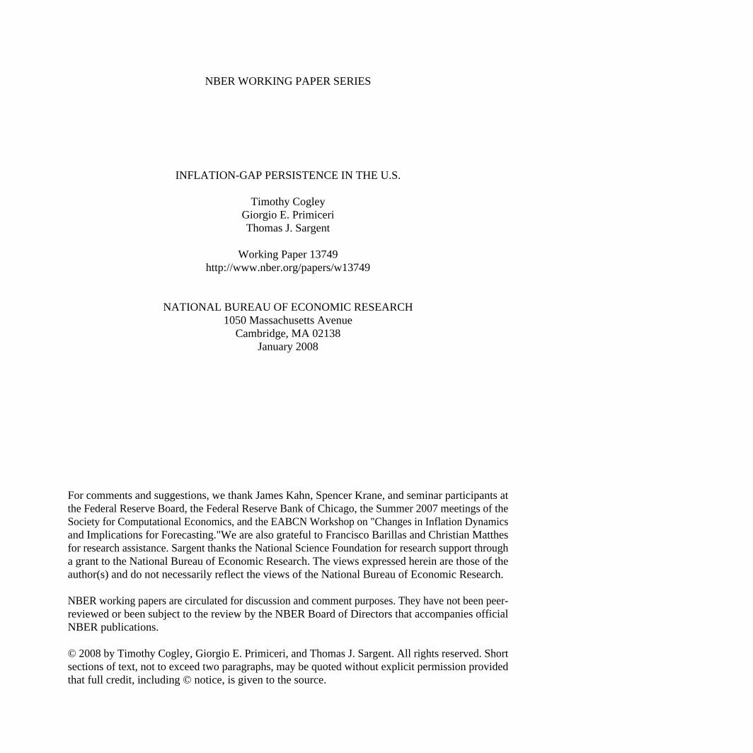
For the AR(1) model, everything depends on a single parameter ρt. Figure 4portrays the posterior median and interquartile range for this parameter for the twoinflation measures.

12

1960 1980 2000

0

0.2

0.4

0.6

0.8

1

GDP Inflation

1960 1980 2000

0

0.2

0.4

0.6

0.8

1

PCE Inflation

Figure 4: Posterior Median and Interquartile Range for ρt

For GDP inflation, the inflation gap is moderately persistent throughout the sam-ple. The median estimate for ρt was around 0.55 in the early 1960s. It increasedgradually to 0.7 by 1980, and then fell in two steps in the early 1980s and early1990s, eventually reaching a value of 0.3 at the end of the sample. These estimatesimply half-lives of 3.5, 5.8, and 1.7 months, respectively. For PCE inflation, the gapwas initially less persistent, with an autocorrelation of 0.3, but otherwise movementsin ρt are similar to those for GDP inflation. The patterns shown here are consistentwith evidence reported in our earlier papers. Taken at face value, the figure suggestsnot only that inflation was lower on average during the Volcker-Greenspan years, butalso that the inflation gap was less persistent.

The controversy about inflation persistence hinges not on the evolution of theposterior median or mean, however, but rather on whether changes in ρt are statis-tically significant. To assess this, we examine the joint posterior distribution for ρt

across pairs of time periods. There are many possible pairs, of course, and to makethe problem manageable we concentrate on two pairs, 1960-1980 and 1980-2004. Theyears 1960 and 2004 are the beginning and end of our sample, respectively.12 Wechose 1980.Q4 because it was the eve of the Volcker disinflation and because it splitsthe sample roughly in half. However, the results reported below are not particularlysensitive to this choice. Dates adjacent to 1980.Q4 tell much the same story.

Figures 5 and 6 depict results for GDP inflation. Figure 5 portrays the joint dis-tribution for ρ1980 and ρ2004, with values for 1980 plotted on the x-axis and those for2004 on the y-axis. Combinations clustered near the 45 degree line represent pairsfor which there was little or no change. Those below the 45 degree line represent adecrease in persistence (ρ1980 > ρ2004), while those above represent increasing per-sistence. Similarly, figure 6 illustrates the joint distribution for ρ1960 and ρ1980, withvalues for 1960 plotted on the x-axis and those for 1980 on the y-axis.

12Earlier data are used as a training sample for the prior.

13

−0.2 0 0.2 0.4 0.6 0.8 1−0.2

0

0.2

0.4

0.6

0.8

1

GDP Deflator

1980

20

04

Figure 5: Joint Distribution for ρ1980 and ρ2004, GDP Inflation

−0.2 0 0.2 0.4 0.6 0.8 1−0.2

0

0.2

0.4

0.6

0.8

1

GDP Deflator

1960

19

80

Figure 6: Joint Distribution for ρ1960 and ρ1980, GDP Inflation

A number of alternative perspectives can be represented on these graphs. Stockand Watson assume ρt = 0, so the point (0, 0) represents their model. There aresome realizations in the neighborhood of the origin, but most of the probability masslies elsewhere. The second column of table 1 reports the probability that ρt is closeto zero in both periods, where ‘close’ is defined as |ρ| < 0.1. This comes out to 1.2and 1.7 percent, respectively, for the two pairs of years. This finding motivates ourextension of their model.

14

Table 1: Posterior ProbabilitiesGDP Inflation

pair Stock-Watson |∆ρ| < 0.05 High, No Change Changing ρ1980, 2004 0.012 0.122 <0.001 0.8941960, 1980 0.017 0.384 0.027 0.758

PCE Inflationpair Stock-Watson |∆ρ| < 0.05 High, No Change Changing ρ

1980, 2004 0.006 0.056 <0.001 0.9591960, 1980 0.008 0.066 <0.001 0.956

Sims (2001), Stock (2001), and Pivetta and Reis (2007) argue that inflation persis-tence is approximately unchanged. That perspective can be represented by drawinga neighborhood along the 45 degree line. As figures 5 and 6 show, the posterior at-taches considerable probability mass to a ridge clustered tightly along the 45 degreeline. How much probability is near that ridge depends on how a neighborhood isdefined. For example, if we define ‘little change’ by the neighborhood |∆ρ| < 0.05,the posterior probability comes to 12 and 38 percent, respectively, for the two pairs ofyears. Obviously these probabilities would be higher if we widened the neighborhoodand lower if we narrowed it, but the point is that the probability is nontrivial evenfor a narrowly defined interval along the 45 degree line. For the GDP deflator, thenotion that univariate inflation-gap persistence is approximately constant cannot berejected at the 10 percent level.

If we examine the ridges more closely, we notice that the scatterplots are densestalong the ridge for low values of ρ and that they become sparse for high values.Thus, the notion that inflation-gap persistence is both unchanging and high has littlesupport. For example, if we define ‘high persistence’ as a half-life of 1 year or more(ρ ≥ 0.8409), the probability of high and unchanging persistence is less than one-tenthof 1 percent for 1980-2004 and 2.7 percent for 1960-1980. Inflation-gap persistencemight have been high (especially during the Great Inflation), or it might have beenunchanged, but it is unlikely that it was both. As noted above, the notion thatpersistence is both high and unchanging really applies to inflation – because of driftin τt – but not to the inflation gap.

In figure 5, the largest probability mass of points – a bit less than 90 percent– lies below the 45 degree line. For combinations in this region, ρ1980 > ρ2004, sothis represents the probability of declining inflation-gap persistence. We interpretthis as substantial though not decisive evidence of a decline in persistence. Similarly,in figure 6, the preponderance of the combinations – approximately 75 percent –lie above the 45 degree line and are consistent with the idea that the inflation gapbecame more persistent between 1960 and 1980.

15

Thus, for GDP inflation the univariate evidence is mixed. While the preponder-ance of the joint distribution points to a rise and then a decline in persistence, thereis enough mass along the 45 degree ridge in figures 5 and 6 to support the idea thatinflation-gap persistence has not changed. This does not mean that the two inter-pretations stand on an equal footing; one has higher posterior probability than theother. But neither perspective overwhelms the other, and neither can be dismissedas unreasonable.

Figures 7 and 8 repeat this analysis for PCE inflation. For this measure, clearevidence emerges of a rise in persistence between 1960 and 1980 and a decline there-after. In figures 7 and 8, the 45 degree ridges are more sparsely populated than thosefor GDP inflation, and the great majority of points lie below or above the line. Theprobability of an increase in ρt between 1960 and 1980 is 0.956, and the probabilityof a decline after 1980 is 0.959. This is significant evidence of changing inflation-gappersistence.

−0.2 0 0.2 0.4 0.6 0.8 1−0.2

0

0.2

0.4

0.6

0.8

1

PCE Deflator

1980

20

04

Figure 7: Joint Distribution for ρ1980 and ρ2004, PCE Inflation

−0.2 0 0.2 0.4 0.6 0.8 1−0.2

0

0.2

0.4

0.6

0.8

1

PCE Deflator

1960

19

80

Figure 8: Joint Posterior for ρ1960 and ρ1980, PCE Inflation

16

4.2.2 A pitfall: uncertainty at one time or across time?

Had we followed the methods of Pivetta and Reis (2007), we would not have de-tected these changes. Pivetta and Reis assess statistical significance by asking whethera horizontal line can be drawn through marginal confidence bands surrounding themean or median. If it can, they conclude that the evidence for change is statisti-cally insignificant. For both GDP and PCE inflation, marginal confidence bands forρt overlap at all three dates. Hence we would have mistakenly concluded that theevidence for changing persistence is insignificant. Their procedure is difficult to in-terpret, however, because it confounds uncertainty about the level of ρt at a point intime with uncertainty about changes in ρt across dates. A marginal confidence bandis fine for assessing level uncertainty at a point in time, but we must consult the jointdistribution across dates in order to assess uncertainty about changes.13 For PCEinflation, the joint distribution points to significant changes in ρt.

4.3 Multivariate evidence

As noted above, the estimates reported in figures 2 and 3 suggest that VARs aremore promising for detecting changes in inflation-gap persistence. Accordingly, wenow turn to multivariate evidence. For each draw in the posterior distribution forVAR parameters, we calculate R2

jt statistics as in equation (18) and then study howthey changed during and after the Great Inflation. Figure 9 portrays the posteriormedian and interquartile range for R2

jt for j = 1, 4, and 8 quarters.The top row refers to 1-quarter ahead forecasts. In the mid 1960s, VAR pseudo

forecasts accounted for approximately 50 to 55 percent of the variation of the inflationgap. During the Great Inflation, this increased to more than 90 percent and at timesapproached 99 percent. The inflation gap became less predictable during the Volckerdisinflation, and after that R2

1t settled to the neighborhood of 50 percent. It was stillaround 50 percent at the end of the sample.

The second and third rows refer to 4 and 8 quarter forecasting horizons. Asexpected, R2

jt statistics are lower for longer horizons. For j = 4, VAR pseudo forecastsaccounted for roughly a quarter of the inflation-gap variation in the mid 1960s, forapproximately 50 to 75 percent during the Great Inflation, and for about 15 percentafter the Volcker disinflation. For j = 8, the numbers follow a similar pattern but arelower. VAR pseudo forecasts accounted for about 10 percent of inflation-gap variationin the mid-1960s, for 20 to 35 percent during the mid 1970s and early 1980s, and for 10percent or less after the Volcker disinflation. Thus, there was apparently a substantialdecline in inflation-gap predictability after the mid 1980s.

13Sims and Zha (1999) make this point in the context of confidence bands for impulse responsefunctions. Their logic applies here.

17

1960 1970 1980 1990 20000

0.5

1

GDP Deflator

1960 1970 1980 1990 20000

0.5

1

1960 1970 1980 1990 20000

0.5

1

1960 1970 1980 1990 20000

0.5

1

PCE Deflator

1960 1970 1980 1990 20000

0.5

1

1960 1970 1980 1990 20000

0.5

1

Figure 9: R2t Statistics

Yet the question remains whether the changes are statistically significant. Weapproach this question in the same way as before, by examining the joint posteriordistribution for R2

jt across pairs of years. Figures 10 and 11 plot the joint distributionfor R2

1t for the years 1980 and 2004. Values for 1980 are shown on the x -axis, andthose for 2004 are on the y-axis. For both measures of inflation, virtually the entiredistribution lies below the 45 degree line, signifying that R2

1,1980 > R21,2004 with high

probability. Very few points are clustered along the 45 degree line.

18

0 0.1 0.2 0.3 0.4 0.5 0.6 0.7 0.8 0.9 10

0.1

0.2

0.3

0.4

0.5

0.6

0.7

0.8

0.9

1

1980

2004

1 Quarter Ahead

Figure 10: Joint Distribution for R21,1980 and R2

1,2004, GDP Inflation

0 0.1 0.2 0.3 0.4 0.5 0.6 0.7 0.8 0.9 10

0.1

0.2

0.3

0.4

0.5

0.6

0.7

0.8

0.9

1

1980

2004

1 Quarter Ahead

Figure 11: Joint Distribution for R21,1980 and R2

1,2004, PCE Inflation

Table 2 records the fraction of posterior draws for which R2jt declined between

1980 and 2004. For 1-step ahead pseudo forecasts, the probability of a decline is98.9 and 97.8 percent, respectively, for GDP and PCE inflation, thus confirming thevisual impression conveyed by the figures. For 4- and 8-quarter ahead forecasts, thejoint distributions are less tightly concentrated than those shown above, and theprobabilities are a bit lower. Nevertheless, at the 4-quarter horizon, the probabilityof a decline in R2

jt is almost 96 percent for GDP inflation and 92 percent for PCEinflation, and they are a bit less than 90 percent at the 8-quarter horizon.

19

Table 2: Probability of Changing R2jt

GDP Inflationpair 1 Quarter Ahead 4 Quarters Ahead 8 Quarters Ahead

1980, 2004 0.989 0.957 0.8891960, 1980 0.991 0.919 0.820

PCE Inflationpair 1 Quarter Ahead 4 Quarters Ahead 8 Quarters Ahead

1980, 2004 0.978 0.922 0.8761960, 1980 0.960 0.857 0.792

Figures 12 and 13 examine changes in predictability between 1960 and 1980.Here we plot R2

1,1960 on the x -axis and R21,1980 on the y-axis. Now virtually the entire

distribution lies above the 45 degree line, signifying that R21,1960 < R2

1,1980 with highprobability. Table 2 also reports the probability of an increase in R2

j,t between 1960and 1980. For GDP inflation, this probability is 99.1 percent for 1-quarter aheadpseudo forecasts, 91.9 percent for 1-year ahead forecasts, and 82 percent for 2-yearahead forecasts. The probabilities are slightly lower for PCE inflation, but the resultsstill point to a significant change in predictability at the 1-quarter horizon.

Thus, statistically significant evidence for changes in inflation persistence emergesfrom VARs. Estimates of R2

1t put posterior probabilities above 96 percent on the jointevent of both an increase in persistence during the Great Inflation and a decline inpersistence after the Volcker disinflation. The results for 4-quarter ahead forecastsalso point in this direction, standing at the 90 or 95 percent levels for a fall inpersistence in the second half of the sample and straddling the 90 percent level fora rise in the first half. The results for 2-year ahead forecasts hint at a change inpersistence, but fall short of statistical significance at the 90 percent level.

0 0.1 0.2 0.3 0.4 0.5 0.6 0.7 0.8 0.9 10

0.1

0.2

0.3

0.4

0.5

0.6

0.7

0.8

0.9

1

1960

1980

1 Quarter Ahead

Figure 12: Joint Distribution for R21,1960 and R2

1,1980, GDP Inflation

20

0 0.1 0.2 0.3 0.4 0.5 0.6 0.7 0.8 0.9 10

0.1

0.2

0.3

0.4

0.5

0.6

0.7

0.8

0.9

1

1960

1980

1 Quarter Ahead

Figure 13: Joint Distribution for R21,1960 and R2

1,1980, PCE Inflation

5 Related research

Barksy (1987) explains an apparent violation of the Fisher equation in prewar USdata in terms of changes in inflation predictability. The correlation between infla-tion and short-term nominal interest was negative prior to World War II but positiveafterward. Barsky argues that this reflects changes in the time-series properties ofinflation, not a change in the structural relation between nominal interest and ex-pected inflation. Although inflation was highly forecastable after the mid 1960s,he documented that it was essentially unforecastable prior to World War I, and hedemonstrated that this could account for the absence of a Fisher correlation in pre-wardata.

Benati (2006) gathers data on inflation in a wide variety of monetary regimesand examines how inflation persistence varies across regime. Broadly speaking, hereports that high persistence occurs only in monetary regimes that lack a well-definednominal anchor. For instance, for the modern era he contrasts countries whose centralbank explicitly targets inflation with those that do not, and he finds that inflationis more autocorrelated in the latter. He also extends Barsky’s work by looking atpre-WWII data from countries other than the US and confirms that inflation wasclose to white noise in many countries.

For the postwar US, Stock and Watson (2007) also document changes in thepredictability of inflation. They find that inflation has become both easier and harderto forecast in the Volcker-Greenspan era. In an absolute sense, forecasting inflation iseasier because inflation is less volatile and its innovation variance is smaller. But in arelative sense, predicting inflation has become more difficult because future inflationis less closely correlated with current inflation and other predictors. Their conclusion

21

agrees with ours: although the innovation variance for inflation has declined, theunconditional variance has fallen by more, implying that predictive R2 statistics arelower.

5.1 Comparison with Atkeson-Ohanian findings

Stock and Watson also interpret a result of Atkeson and Ohanian (2001) in termsof the changing time-series properties of inflation. Atkeson and Ohanian studiedthe predictive power of backward-looking Phillips-curve models during the Volcker-Greenspan era and found that Phillips-curve forecasts were inferior to a naive forecastthat equates expected inflation over the next 12 months with the simple average ofinflation over the previous year. Stock and Watson show that Phillips-curve modelswere more helpful during the Great Inflation, and they account for the change bypointing to two features of the data. First, like many macroeconomic variables,unemployment has become less volatile since the mid-1980s. Hence there is lessvariation in the predictor. Second, the coefficients linking unemployment and otheractivity variables to future inflation have also declined in absolute value, furthermuting their predictive power.

Our VARs share these characteristics. In figure 14 , we illustrate how news aboutunemployment alters forecasts of inflation. At each date, we imagine that forecastersstart with information on inflation, unemployment, and the nominal interest ratethrough date t − 1 and then see a one-sigma innovation in unemployment. Theyrevise their inflation forecasts in light of the unemployment news. Because the VARinnovations are correlated, the forecast revision at horizon j is14

FRjt = eπAjtE(εzt|εut)σut. (19)

Since the innovations are conditionally normal and the unemployment innovation isscaled to equal σut, E(εzt|εut) = cov(εzt, εut)/σut. The figure portrays the median andinterquartile range for forecast revisions at horizons of 1, 4, and 8 quarters.

For the most part, a positive innovation in unemployment reduces expected infla-tion. Furthermore, in the 1970s and early 1980s, the magnitude of forecast revisionswas substantial. For instance, according to the median estimates, a one-sigma inno-vation in unemployment would have reduced expected inflation 4 quarters ahead byclose to 50 basis points in the mid-1970s and by approximately 1 to 1.5 percentagepoints at the time of the Volcker disinflation. After the mid 1980s, however, thesensitivity of inflation forecasts to unemployment news was more muted. During theGreenspan era, a one-sigma innovation in unemployment would have had essentiallyno influence at all on inflation forecasts one or two years ahead.

14This follows from another anticipated-utility approximation.

22

1960 1970 1980 1990 2000−1.5

−1

−0.5

0

GDP Inflation

1 Q

ua

rte

r

1960 1970 1980 1990 2000

−1.5

−1

−0.5

0

4 Q

ua

rte

rs

1960 1970 1980 1990 2000−1.5

−1

−0.5

0

8 Q

ua

rte

rs

1960 1970 1980 1990 2000−1.5

−1

−0.5

0

PCE Inflation

1960 1970 1980 1990 2000

−1.5

−1

−0.5

0

1960 1970 1980 1990 2000−1.5

−1

−0.5

0

Figure 14: How Unemployment News Alters Expected Inflation

As Stock and Watson point out, these outcomes reflect both that unemploymentinnovations are less volatile and that inflation forecasts are less sensitive to innova-tions of a given size. Figure 15 depicts the posterior median and interquartile rangefor σut, the standard deviation of innovations to unemployment. The magnitude ofunemployment innovations was largest at the beginning of the sample and aroundthe time of the Volcker disinflation, but it declined sharply after the mid 1980s. Onereason why unemployment news has become less relevant for inflation forecasting isthat there is less of it.

But this is not the whole story. Figure 16 adjusts for changes in the innovationvariance by showing forecast revisions for the time-series average of the median esti-mate of σut shown in figure 15. This holds the size of the hypothetical unemploymentinnovation constant across dates. Although less pronounced, the pattern shown hereis similar to that depicted in figure 14 (the two figures are graphed on the same scale).Hence figure 14 cannot be explained solely by changes in σut. Especially at horizons

23

of a 4 or 8 quarters, inflation forecasts have also become less sensitive to a givenamount of unemployment news than they were during the Great Inflation.

1960 1980 20000

0.2

0.4

0.6

0.8

1

x 10−3 GDP Inflation

1960 1980 20000

0.2

0.4

0.6

0.8

1

x 10−3 PCE Inflation

Figure 15: Standard Deviation of Unemployment Innovations

1960 1970 1980 1990 2000−1.5

−1

−0.5

0

GDP Inflation

1 Q

ua

rte

r

1960 1970 1980 1990 2000

−1.5

−1

−0.5

0

4 Q

ua

rte

rs

1960 1970 1980 1990 2000−1.5

−1

−0.5

0

8 Q

ua

rte

rs

1960 1970 1980 1990 2000−1.5

−1

−0.5

0

PCE Inflation

1960 1970 1980 1990 2000

−1.5

−1

−0.5

0

1960 1970 1980 1990 2000−1.5

−1

−0.5

0

Figure 16: Forecast Revisions with σu Held Constant

24

Ironically, the decreased predictive power of unemployment innovations for infla-tion coincided with a return of the Phillips correlation. Figure 17 portrays a numberof conditional and unconditional correlations for inflation and unemployment.15 Theunconditional correlation – shown in the bottom row – was negative prior to the 1970s,but it turned positive during the Great Inflation. A negative correlation reappearedafter the Volcker disinflation and has hovered around -0.25 ever since.

1960 1970 1980 1990 2000

−0.4

−0.2

0

GDP Inflation

1 S

tep

1960 1970 1980 1990 2000−0.8−0.6−0.4−0.2

0

4 S

tep

s

1960 1970 1980 1990 2000

−0.6−0.4−0.2

0

8 S

tep

s

1960 1970 1980 1990 2000

−0.5

0

0.5

Un

co

nd

itio

na

l

1960 1970 1980 1990 2000

−0.4

−0.2

0

PCE Inflation

1960 1970 1980 1990 2000−0.8−0.6−0.4−0.2

0

1960 1970 1980 1990 2000−0.6−0.4−0.2

00.20.4

1960 1970 1980 1990 2000

−0.5

0

0.5

Figure 17: Conditional and Unconditional Phillips Correlations

The other rows of the figure depict conditional correlations at forecast horizonsof 1, 4, and 8 quarters. The 1- and 4-quarter ahead forecasts are most relevant for

15These were calculated using the approximations in equations (16) and (17).

25

reconciling conventional wisdom with Atkeson and Ohanian. At these horizons, con-ditional correlations have indeed been negative throughout the sample, peaking inmagnitude at the time of the Volcker disinflation. They are smaller now than in thepast, but at the 4-quarter horizon the correlation is still around -0.25. Nevertheless,these conditional correlations are irrelevant for prediction because they summarizeunexpected comovements in the two variables. That prediction errors in unemploy-ment are inversely related with prediction errors in inflation tells us little about fore-castable movements in the two variables. Thus, Atkeson and Ohanian’s observationsabout predictability can coexist comfortably with conventional views about Phillipscorrelations.

Contrary to Atekson and Ohanion, figures 9-11 suggest that some short-termpredictability remains at the end of the sample. Two caveats should be kept in mind,however. One is that our calculations involve pseudo forecasts that depend on dataand estimates through the end of the sample, while Atkeson and Ohanian look atreal-time, out-of-sample forecasts. Presumably this matters only slightly at the endof the sample, but more for earlier periods.

The other caveat is that there is substantial uncertainty about R22004. We can

state with confidence that R22004 is smaller than R2

1980, but that is mainly because theposterior for R2

1980 clusters tightly near 1. It is harder to say how predictable inflationis at the end of the sample. At the 1-quarter horizon, the probability that R2

2004

exceeds 0.25 is 0.904 for GDP inflation and 0.924 for PCE inflation. Thus, althoughour estimates suggest more predictability than those of Atkeson and Ohanian, the factthat the posteriors portrayed in figures 10 and 11 assign non-negligible probability tovalues of R2

2004 near zero provides at least some weak support for their point of view.

6 A More Structural Analysis

In this section we offer a structural explanation of the statistical findings pre-sented above. We estimate a New-Keynesian model along the lines of Rotemberg andWoodford (1997) and Boivin and Giannoni (2006). This model is a simple possibleframework for addressing the causes of the declines in the volatility, persistence, andpredictability of inflation.

6.1 The model

The model economy is populated by a representative household, a continuum ofmonopolistically competitive firms, and a government. The representative householdmaximizes

Et

∞∑s=0

δsbt+s

[log (Ct+s − hCt+s−1)− ϕ

∫ 1

0

Lt+s (i)1+ν

1 + νdi

], (20)

26

subject to a sequence of budget constraint

∫ 1

0

Pt (i) Ct (i) di + Bt + Tt ≤ Rt−1Bt−1 + Πt +

∫ 1

0

Wt (i) Lt (i) di. (21)

Bt represents government bonds, Tt denotes lump-sum taxes and transfers, Rt is thegross nominal interest rate, and Πt are the profits that firms pay to the household.Ct is a Dixit-Stigliz aggregator of differentiated consumption goods,

Ct =

[∫ 1

0

Ct(i)1

1+θt di

]1+θt

. (22)

Pt is the associated price index, Lt (i) denotes labor of type i that is used to producedifferentiated good i, and Wt (i) is the corresponding nominal wage. The coefficientsh and ν set the degree of internal habit formation and the inverse Frisch elasticityof labor supply, respectively. Finally, bt and θt are exogenous shocks that follow thestochastic processes

log bt = ρb log bt−1 + εb,t (23)

log θt = (1− ρθ) log θ + ρθ log θt−1 + εθ,t.

The random variable bt is an inter-temporal preference shock perturbing the discountfactor, and θt can be interpreted as a shock to the firms’ desired mark-up.

Each differentiated consumption good is produced by a monopolistically compet-itive firm using a linear production function,

Yt(i) = AtLt(i), (24)

where Yt (i) denotes the production of good i, and At represents aggregate laborproductivity. We model At as a unit root process with a growth rate zt ≡ log(At/At−1)that follows the exogenous process

zt = (1− ρz)γ + ρzzt−1 + εz,t. (25)

As in Calvo (1983), at each point in time a fraction ξ of firms cannot re-optimizetheir prices and simply indexes them to the steady-state value of inflation. Subject tothe usual cost-minimization condition, a re-optimizing firm chooses its price (Pt(i))by maximizing the present value of future profits,

Et

∞∑s=0

ξsδsλt+s

{Pt(i)π

sYt+s(i)−Wt+s (i) Lt+s(i)}

, (26)

where π is the gross rate of inflation in steady state and λt+s is the marginal utilityof consumption.

27

The monetary authority sets short-term nominal interest rates according to aTaylor rule,

Rt

R=

(Rt−1

R

)ρR

[(π4,t

(π∗t )4

)φπ4

(Yt

Y ∗t

)φY

]1−ρR

eεR,t . (27)

The central bank smooths interest rates and responds to two gaps, the deviation ofannual inflation (π4,t) from a time-varying inflation target and the difference betweenoutput and its flexible price level. R is the steady-state value for the gross nominalinterest rate and εR,t is a monetary policy shock that we assume to be i.i.d.

Following Ireland (2007), we model the inflation target π∗t as an exogenous randomprocess,

log π∗t = (1− ρ∗) log π + ρ∗ log π∗t + ε∗,t. (28)

There are many reasons that the Central Bank’s inflation target might vary overtime. Our preferred one is that the central bank endogenously adjusts its target as itlearns about the structure of the economy. For instance, Sargent (1999), Cogley andSargent (2005), Primiceri (2006), and Sargent, Williams, and Zha (2006) hypothesizethat changing beliefs about the output-inflation tradeoff generated a pronouncedlow-frequency, hump-shaped pattern in inflation. We approximate outcomes of thislearning process by an exogenous random variable like (28).16

6.2 Model solution and observation equation

Since the technology process At is assumed to have a unit root, consumption, realwages, and output evolve along a stochastic growth path. To solve the model, we firstrewrite it in terms of deviations of these variables from the technology process. Thenwe solve the log-linear approximation of the model around the non-stochastic steadystate. We specify the vector of observable variables as [log Yt − log Yt−1, πt, Rt]. Forestimation, we use data on per-capita GDP growth, the quarterly growth rate of theGDP deflator, and the Federal funds rate.17

6.3 Bayesian inference and priors

We use Bayesian methods to characterize the posterior distribution of the model’sstructural parameters.18 Table 3 reports our priors. These priors are relatively dis-perse and are broadly in line with those adopted in previous studies (see, for instance,Del Negro et al. 2007 or Justiniano and Primiceri 2007). But a few items deservediscussion.

16By way of analogy, technology is also endogenous, but macroeconomists often model it as anexogenous random variable.

17These variables are standard for estimating small-scale DSGE models (see, for instance, Boivinand Giannoni 2006).

18See appendix B.

28

Table 3: Priors for Structural Parameters

Coefficient Prior

νθ − 1100γ

100 (π − 1)100 (δ−1 − 1)

hξφπ

φy

ρR

ρz

ρθ

ρ∗ρb

100σR

100σz

100σθ

100σ∗100σb

Density Mean Standard DeviationCalibrated 2 −Calibrated 0.1 −Normal 0.475 0.025Normal 0.5 0.1Gamma 0.25 0.1

Beta 0.5 0.1Beta 0.66 0.1

Normal 1.7 0.3Gamma 0.3 0.2

Beta 0.6 0.2Beta 0.4 0.2Beta 0.6 0.2

Calibrated 0.995 −Beta 0.6 0.2

Inverse Gamma 0.15 1Inverse Gamma 1 1Inverse Gamma 0.15 1

Uniform 0.075 0.0433Inverse Gamma 1 1

• We fix two parameters because they are not identified. In particular, we set theFrisch elasticity of labor supply (1/ν) to 0.5 and the steady-state price mark-up(θ − 1) to 10%.

• For all but two persistence parameters, we use a Beta prior with mean 0.6and standard deviation 0.2. One exception concerns labor productivity, whichalready includes a unit root. For this reason, we center the prior for the autocor-relation of its growth rate (ρz) at 0.4. The other exception is the autocorrelationof the inflation target shock, which we calibrate to 0.995. In other words, werestrict π∗t so that it captures low-frequency movements in inflation.19

• The standard deviation of the innovation to the inflation target is a crucialparameter in our analysis because it governs the rate at which π∗t drifts. Wewant a weakly informative prior in order to let the data dominate the posterior.Accordingly, we adopt a uniform prior on (0,0.15). For the standard deviationsof the other shocks, we follow Del Negro et al. (2007) by choosing priors that

19We do not set ρ∗ = 1 because the DSGE model would not admit a non-stochastic steady stateand the log-linearization would not be possible in that case.

29

are fairly disperse and that generate realistic volatilities for the endogenousvariables.

• Finally, we truncate the prior at the boundary of the determinacy region.

6.4 Estimation Results

We estimate the model separately on two subsamples. The first, 1960:I - 1979:II,corresponds approximately to the period of rising inflation before the Volcker chair-manship. The second period, 1982:IV - 2006:IV, corresponds to the Volcker andGreenspan chairmanships, excluding the years of monetary targeting, for which theTaylor rule might not represent an appropriate description of systematic monetarypolicy (see, for instance, Sims and Zha 2006 or Hanson 2006).

Figure 18 presents the model-implied evolution of the Central Bank inflation ob-jective. Notice that it resembles quite closely the VAR-based estimate of the perma-nent component of inflation plotted in figure 1.

1960 1965 1970 1975 1980 1985 1990 1995 2000 20050

2

4

6

8

10

12

14GDP deflatorπ*

Figure 18: The Central Bank’s Inflation Target

Table 4 reports estimates of the structural parameters. While many coefficientsare similar across subsamples, there are some important differences. For example,we find that the Taylor-rule coefficient for inflation (φπ) increased from 1.55 in thefirst subsample to 1.78 in the second. While an increase is consistent with findings ofClarida, Gali, and Gertler (2000) and Lubik and Schorfheide (2004), we do not findvalues of φπ in the pre-1980 period as low as they do. This might be due to the factthat, for simplicity, we have ruled out indeterminacy a priori. Another possibility isthat the presence of a time varying inflation target reduces the differences betweenthe reaction to inflation in the two subsamples.

30

Table 4: Posteriors for Structural Parameters

Coefficient 1960-1979 1982-2006

100γ100 (π − 1)

100 (δ−1 − 1)hξφπ

φy

ρR

ρz

ρθ

ρb

100σR

100σz

100σθ

100σ∗100σb

Median 25th pct 75th pct0.468 0.452 0.4840.501 0.435 0.5660.159 0.121 0.2040.445 0.390 0.5020.782 0.741 0.8181.557 1.372 1.7460.643 0.541 0.7720.704 0.630 0.7590.264 0.156 0.3900.598 0.515 0.6760.699 0.632 0.7580.160 0.147 0.1740.641 0.527 0.7970.118 0.097 0.1390.081 0.062 0.1042.533 2.226 2.889

Median 25th pct 75th pct0.484 0.467 0.5000.516 0.452 0.5810.255 0.199 0.3190.526 0.482 0.5680.800 0.762 0.8351.784 1.598 1.9740.66 0.562 0.7840.633 0.576 0.6860.297 0.191 0.4150.255 0.182 0.3440.876 0.850 0.8980.069 0.063 0.0760.493 0.426 0.5620.126 0.114 0.1370.049 0.037 0.0652.429 2.146 2.785

A second notable change in monetary policy concerns the innovation variances forthe two shocks, ε∗,t and εR,t. According to our estimates, both declined substantiallyafter the Volcker disinflation. The innovation variance for the shock to target inflationfell by almost 50 percent, from 0.081 to 0.049, while the variance for the funds-rate shock declined even more, from 0.16 to 0.07. The decline in σ∗ should not besurprising, given the findings of Stock and Watson (2007) and our VAR statisticalresults. It contributes directly to the decline in inflation volatility after 1980.

Among the nonpolicy parameters, most change only slightly across the two sam-ples. This is comforting because these parameters are supposed to be invariant tochanges in monetary policy. One exception is the persistence parameter ρθ for thecost-push shock, which declines from 0.6 to 0.25. Thus, the cost-push shock is lesspersistent and has smaller unconditional variance after 1982. This decline might re-flect the reduced incidence of oil-price shocks in the second half of the period. If thatis correct, the estimates capture elements of good luck as well as improved policy.

Table 5 summarizes the model’s implications for inflation volatility, persistence,and predictability at the posterior median of the model parameters. Column 1 re-ports the unconditional standard deviation of inflation, while columns 2−4 report R2

statistics for inflation-gap predictability for forecasting horizons of 1, 4 and 8 quar-ters.20 Notice that, in line with our statistical VAR findings, the model reproduces

20The inflation gap here is defined as the difference between inflation and the central bank inflation

31

well the substantial decline in volatility, persistence and predictability of inflation.All decrease by roughly 50 to 70 percent.21

Table 5: Implications of the DSGE Model for Inflation Volatility andPredictability

100 · std (πt) R21 R2

4 R28 Slope

1960:I - 1979:II 4.702 0.631 0.433 0.409 0.1321982:IV - 2006:IV 2.354 0.206 0.136 0.124 0.040Percent Change −50 −67 −69 −70 −70

Finally, column 5 addresses the results of Atkeson and Ohanian (2001). Here wereport the model-implied slope β of the Phillips curve,

Et

(π4,t+4 − π4,t

)= β

(Yt − Y ∗

t

)+ εt,t+4.

We do not include a constant because the variables of the regression all have meanzero in the model. Except for the fact that we replace the unemployment rate withthe output gap, this is the regression estimated by Atkeson and Ohanian (2001).Consistent with their results, those of Stock and Watson, and our own results reportedabove, our model implies a substantial decline in the predictive power of real-activityvariables in conventional Phillips curve regressions after the Volcker disinflation.

6.5 Counterfactuals

In line with the statistical VAR findings, the DSGE model reproduces much ofthe substantial decline in volatility, persistence, and predictability of inflation. Weare sufficiently encouraged by its performance to use the DSGE model to explore thestructural sources of these changes.

In this subsection, we conduct some counterfactual exercises in order to under-stand the causes of the decline in inflation volatility, persistence, and predictability.In the first experiment, we combine the Taylor-rule coefficients ([φπ, φy, ρR, σR, σ∗])of the second subsample with the private-sector parameters of the first. In this way,we assess the extent to which better monetary policy would have reduced inflationvolatility and persistence during the Great Inflation. In the second experiment, wecombine the private-sector parameters of the second subsample with the policy pa-rameters of the first. This scenario illustrates the contribution of nonpolicy factorsto the improvement in inflation outcomes.

objective that, in the DSGE model, captures the permanent component of inflation.21Since we estimate the model on two separate subsamples, the joint posterior distribution of the

coefficients of the first and second subsample is not available. Therefore, we cannot report standarderrors.

32

Table 6 reports the results. The numbers recorded there represent the proportionof the total change across subsamples accounted for by the hypothetical structuralshift,

100× counterfactual change

total change.

Positive numbers signify that the counterfactual goes in the same direction as thetotal change, and negative numbers mean that it goes in the opposite direction.

Table 6: Counterfactual Exercises Based on the DSGE Model

Coefficients volatilitypersistenceR2

1 R24 R2

8

Slope (β)

Policy 2, Private 1 75 43 90 91 -94σ∗ 69 32 68 69 -46φπ 9 13 28 28 -27

Private 2, Policy 1 36 43 15 14 125ρθ 7 -39 -109 -111 121

Monetary policy seems to be the most important factor behind the decline ininflation volatility. The change in policy rule accounts for 75 percent of the decline ininflation volatility. In contrast, better luck – primarily in the form of a less volatileand persistent cost-push shock – accounts for 36 percent of the decline. This is asubstantial contribution, but only about half the magnitude of the effect of monetarypolicy.22

The results for predictability are similar, especially at the 4 and 8 quarter horizons.At those horizons, better monetary policy accounts for approximately 90 percent ofthe decline, while changes in private-sector behavior account for around 15 percent.At the 1-quarter horizon, however, the two factors contribute equally to the declinein predictability, each accounting for 43 percent of the total change.

The second and third rows of the table 6 look more closely at particular aspectsof monetary policy. Here we change a single Taylor-rule parameter, holding all othercoefficients equal to the estimated value from subsample 1. Otherwise the experimentsare the same as before.

Among monetary-policy coefficients, changes in the variability of the inflationobjective (σ∗) and in the reaction to inflation (φπ) have the largest impact on inflationoutcomes. The more stable inflation objective is responsible for the largest portion ofthe decline in inflation volatility and persistence, accounting for roughly two-thirds

22The two numbers need not sum to 100 because the model is nonlinear in the coefficients and,therefore, the total change is not the sum of the effects of the policy and nonpolicy coefficients shift.

33

of the total change. This is because changes in the Central Bank’s inflation targetgenerate persistent deviations of the nominal interest rate and marginal cost from thesteady state. In turn, this induces persistent deviations of inflation from the target,i.e., a persistent component in the inflation-gap. Hence, a decline in the volatility ofthe inflation target reduces the overall persistence of the inflation-gap by reducingthe relative importance of the persistent component.

Another important contributor is stronger monetary-policy reaction to inflation.In our model, however, this is secondary to enhanced stability of the inflation target,accounting for about 10 percent of the decline in volatility and 13-28 percent of thedecline in predictability. One reason that we might be finding a smaller contributionthan has been found by others (e.g., Benati and Surico 2007) is that we truncate ourprior on the boundary of the determinacy region. Thus, our feedback parameter risesfrom 1.56 to 1.78. Enhanced feedback plays a role in our model, but not the primaryrole.

We also look more closely at the particular aspects of private-sector behaviorthat have the greatest influence on changing inflation outcomes. Among nonpolicyparameters, the key change is the shift in the persistence of the mark-up shock. Thefinal row of table 6 sheds light on its contribution. Everything else equal, the declinein persistence of the mark-up shock (ρθ) would have induced an increase in inflation-gap persistence. This might seem surprising but has a simple explanation: a reductionin ρθ corresponds to a decrease in the unconditional variability of the mark-up shock,which reduces the volatility of inflation due to this shock. As a consequence, the roleof the inflation-target shock for inflation becomes relatively larger, and this increasespersistence.

The final column of table 6 examines how changes in monetary policy and private-sector parameters contribute to the flattening of the slope in an Atkeson-Ohanianregression. Recall that the DSGE model predicts a decline in β from 0.13 to 0.04across the two subsamples. In this case, the relative importance of better policyand better luck are reversed. Changes in private sector parameters go in the rightdirection and overpredict the total decline. Conditional on the mark-up shock, theoutput gap and future changes in the inflation rate comove positively. The drop inpersistence and unconditional volatility of the mark-up shock reduces this positivecomovement and results in a lower estimate of the slope coefficient. But changes inpolicy parameters go in the wrong direction and predict a substantial increase in β.Thus, for a complete picture of the change in inflation outcomes, both private andpolicy factors are needed.

34

7 Concluding remarks

This paper reports what autoregressions with drifting coefficients and stochasticvolatility say about the persistence of the inflation gap defined as the fraction of vari-ation of future inflation gaps that is due to past shocks. A high proportion meansthat past shocks retain influence for a long time, while a low proportion signifies thattheir influence decays quickly. Since past shocks give rise to forecastable variationin future inflation gaps, our concept of persistence is closely related to predictability.VAR estimates point to a statistically significant increase in inflation-gap predictabil-ity during the Great Inflation and to a statistically significant decline in predictabilityafter the Volcker disinflation. Univariate estimates are mixed, with significant evi-dence of a rise and fall in persistence for PCE inflation and marginal evidence forGDP inflation.

We have used a new Keynesian DSGE model to examine what caused thesechanges. We find evidence that both better policy and better luck – in the formof less volatile and less persistent cost-push shocks – contributed to improved infla-tion outcomes. The enhanced stability of the Fed’s long-run inflation target standsas key improvement in policy. In our DSGE model, this is the single most importantfactor behind the reduction in inflation volatility and persistence.

The DSGE model treats the inflation target as an exogenous random process.Explaining why it drifts is a priority for future research. Our preferred story involveslearning and changing central bank beliefs about the structure of the economy (Cogleyand Sargent 2005b, Primiceri 2006, and Sargent, Williams, and Zha 2006), but morework is needed to understand this aspect of monetary policy.

A Markov chain Monte Carlo algorithm for simu-

lating the VAR posterior

For the VAR, the posterior density is23

p(θT , HTy , HT

s , By, Bs, σy, σs|Y T ). (29)

The state and measurement innovation variances are defined as

Qt = (B−1s )′Hst(B

−1s ), (30)

Rt = (B−1y )′Hyt(B

−1y ),

respectively, where Hst and Hyt are diagonal matrices with univariate stochasticvolatilities along the main diagonal and Bs and By are triangular matrices with

23The MCMC algorithm for the univariate AR is a special case of that for the VAR.

35

ones along the main diagonal and static covariance parameters below. The univari-ate stochastic volatilities are geometric random walks; the vectors σs and σy list theirinnovation variances. The notation xT represents the complete history of xt.

We use a ‘Metropolis-within-Gibbs’ algorithm to simulate the posterior. Theparameters are partitioned into 7 blocks:

• θT |HTy , HT

s , By, Bs, σy, σs, YT

• HTy |θT , HT

s , By, Bs, σy, σs, YT

• By|θT , HTy , HT

s , Bs, σy, σs, YT

• σy|θT , HTy , HT

s , By, Bs, σs, YT

• HTs |θT , HT

y , By, Bs, σy, σs, YT

• Bs|θT , HTy , HT

s , By, σy, σs, YT

• σs|θT , HTy , HT

s , By, Bs, σy, YT

After substituting Qt for Q, the samplers for the first four blocks are identical tothose in Cogley and Sargent (2005a); details can be found there. Those for the lastthree blocks – which pertain to the state innovation variance Qt – are isomorphic tothe three blocks for the measurement innovation variance Rt. Thus, the appendicesin Cogley and Sargent (2005a) cover those blocks as well.

We executed 100,000 scans of the chain and diagnosed convergence by inspectingrecursive mean plots of the parameters. We discarded the first 50,000 scans to allowfor burn in. The results reported in the text are based on the remaining 50,000 scans.

A.1 Priors for the VAR

The priors are similar to those in Cogley and Sargent (2005a). We assume that thehyperparameters and initial value of the drifting parameters are independent acrossblocks, so that the joint prior factors into a product of marginal priors. Each of themarginal priors is selected from a family of natural conjugate priors and is specifiedto proper yet weakly informative.

The unrestricted prior for the initial state is Gaussian,

f(θ0) ∝ N (θ, P ), (31)

where θ and P are the OLS point estimate and asymptotic variance, respectively,based on a training sample covering the period 1948-58. Because the training sampleis short, the asymptotic variance is large, making the prior weakly informative for θ0.

36

Priors for the blocks governing Rt are also calibrated to put considerable weighton sample information. The prior for H ii

y0 is log-normal,

f(ln H ii

y0

)= N (ln Rii

0 , 10), (32)

where ln Rii0 is the estimate of the log of residual variance of variable i from the

preliminary sample. A variance of 10 is huge on a log scale and allows a wide rangeof values for hi0. As is the case for θ0, the prior mean for Hy0 is no more than aballpark number surrounded by considerable uncertainty.

Similarly, the prior for βy is normal with mean zero and a large variance,

f (β) = N (0, 10000 · I). (33)

Lastly, the prior for σ2yi, the variance of the stochastic volatility innovations, is inverse-

gammaf(σ2

i ) = IG(δi/2, 1/2), (34)

with scale parameter δ = 0.0001 and degree-of-freedom parameter equal to 1. Thisdistribution is proper but has fat tails.

The priors for the blocks governing Qt parallel those for Rt. The prior for H iQ0 is

also log-normal,f

(ln H ii

Q0

)= N (ln Qii

0 , 10), (35)

where Q0 = γ2P is calibrated in the same way as in Cogley and Sargent (2005a).Similarly, the priors for βQ and σQ have the same form as those for βy and σy. Wejust alter the dimensions so that they conform to HQt instead of HRt. The prior meanfor HQ0 induces only a slight degree of time variation in θt, but in other respects thepriors are sufficiently uninformative that they permit a wide range of outcomes forQt.

B Markov chain Monte Carlo algorithm for simu-

lating the DSGE posterior

As in An and Schorfheide (2006), we use a Metropolis-Hastings algorithm tosimulate the posterior distribution of the coefficients of the DSGE model. Let yT

denote the set of available data and α the vector of coefficients of the DSGE model.Moreover, let α(j) denote the jth draw from the posterior of α. The subsequent drawis obtained by drawing a candidate value, α, from a Gaussian proposal distributionwith mean α(j) and variance s · V . We then set α(j+1) = α with probability equal to

min

{1,

p(α|yT

)

p (α(i)|yT )

}. (36)

37

If the proposal is not accepted, we set α(j+1) = α(j).The posterior distribution for α, p

(α|yT

), can be computed multiplying the

prior density by the likelihood function. Because the DSGE model has a linear-Gaussian state-space representation, the likelihood function can be evaluated usingthe prediction-error decomposition and the Kalman filter.

The algorithm is initialized around the posterior mode, found using a standardmaximization algorithm. We set V to the inverse Hessian of the posterior evaluatedat the mode, while s is chosen in order to achieve an acceptance rate approximatelyequal to 25 percent. We run two chains of 70,000 draws and discard the first 20,000to allow convergence to the ergodic distribution.

ReferencesAn, S. and F. Schorfheide, 2007, Bayesian Analysis of DSGE Models, Econometric

Reviews 39, 1357-1373.

Atkeson, A. and L.E. Ohanian, 2001, Are Phillips Curves Useful for ForecastingInflation? Federal Reserve Bank of Minneapolis Quarterly Review 25, 2-11.

Barsky, R.B., 1987, The Fisher Hypothesis and the Forecastability and Persistenceof Inflation, Journal of Monetary Economics 19, 3-24.

Benati, L., 2006, Investigating Inflation Persistence Across Monetary Regimes,unpublished manuscript, European Central Bank.

Benati, L. and P. Surico, 2007, U.S. Evolving Monetary Policy and the InflationGap’s Persistence and Predictability, mimeo, European Central Bank.

Beveridge, S., and C.R. Nelson, 1981. A New Approach to Decomposition ofEconomic Time Series into Permanent and Transitory Components with ParticularAttention to Measurement of the Business Cycle. Journal of Monetary Economics 7,151-174.

Bayer A. and R. Farmer, 2007, On the Indeterminacy of Determinacy and Inde-terminacy: Comments on the Paper “Testing for Indeterminacy” by Thomas Lubikand Frank Schorfheide, American Economic Review 97(1), 524-529.

Boivin, J. and M. Giannoni, 2006, Has Monetary Policy Become More Effective?,Review of Economics and Statistics 88(3), 445-462.

Calvo, G., 1983, Staggered Prices in a Utility-Maximizing Framework, Journal ofMonetary Economics, 12(3), 383-398.

Clarida, R., J. Gali and M. Gertler, 2000, Monetary Policy Rules and Macroeco-nomic Stability: Evidence and Some Theory, The Quarterly Journal of Economics115(1), 147-180.

Cogley, T. and T.J. Sargent, 2001, Evolving Post World War II U.S. InflationDynamics, NBER Macroeconomics Annual 16, 331-373.

38

Cogley, T. and T.J. Sargent, 2005a, Drifts and Volatilities: Monetary Policies andOutcomes in the Post War U.S., Review of Economic Dynamics 8, 262-302.

Cogley, T. and T.J. Sargent 2005b. The Conquest of U.S. Inflation: Learning andRobustness to Model Uncertainty. Review of Economic Dynamics 8, 528-563.

Cogley, T. and T.J. Sargent, 2006, Anticipated Utility and Rational Expecta-tions as Approximations of Bayesian Decision Making, forthcoming, InternationalEconomic Review.

Cogley, T., S. Morozov, and T.J. Sargent, 2005, Bayesian Fan Charts for U.K.Inflation: Forecasting and Sources of Uncertainty in an Evolving Monetary System,Journal of Economic Dynamics and Control 29, 1893-1925.

Cogley, T. and A.M. Sbordone, 2006, Trend Inflation and Inflation Persistence inthe New Keynesian Phillips Curve, unpublished manuscript.

Del Negro, M., F. Schorfheide, F. Smets and R. Wouters, 2007, On the Fit andForecasting Performance of New Keynesian Models, Journal of Business and Eco-nomic Statistics 25(2), 123-162.

Diebold, F.X. and L. Kilian, 2001, Measuring Predictability: Theory and Macroe-conomic Applications, Journal of Applied Econometrics 16, 657-669.

Gelfand, A.E. Model determination using sampling-based methods. In W.R. Gilks,S. Richardson, and D.J. Spiegelhalter, eds., Markov Chain Monte Carlo in Practice,London: Chapman and Hall, 1996.

Hanson, M.S., 2006, Varying Monetary Policy Regimes: A Vector AutoregressiveInvestigation, Journal of Economics and Business, Elsevier 58(5-6), 407-427.

Ireland, P.N., 2007, Changes in the Federal Reserve’s Inflation Target: Causesand Consequences, forthcoming, Journal of Money Credit and Banking.

Justiniano, A. and G.E. Primiceri, 2007, The Time-Varying Volatility of Macroe-conomic Fluctuations, forthcoming, American Economic Review.

Kreps, D., 1998, Anticipated Utility and Dynamic Choice, 1997 Schwartz Lecture,in Frontiers of Research in Economic Theory, Edited by D.P. Jacobs, E. Kalai, andM. Kamien, Cambridge University Press, Cambridge, England.

Levin, A.T. and J.M. Piger, 2004, Is Inflation Persistence Intrinsic in IndustrialSocieties?, ECB working paper no. 334.

Lubik T.A. and F. Schorfheide, 2004, Testing for Indeterminacy: An Applicationto U.S. Monetary Policy, American Economic Review, 94(1), 190-217.

Pivetta, F. and R. Reis, 2007, The Persistence of Inflation in the United States,Journal of Economic Dynamics and Control 31, 1326-58.

Primiceri, G., 2005, Time Varying Structural Vector Autoregressions and Mone-tary Policy, Review of Economic Studies 72, 821-852.

39

Primiceri, G., 2006, Why Inflation Rose and Fell: Policymakers’ Beliefs and U.S.Postwar Stabilization Policy, Quarterly Journal of Economics 121, 867-901.

Rotemberg J.J. and M. Woodford, 1997, An Optimization-Based EconometricModel for the Evaluation of Monetary Policy, NBER Macroeconomics Annual 12,297-346.

Sargent, T.J., N. Williams and T. Zha, 2006, Shocks and Government Beliefs: TheRise and Fall of American Inflation, American Economic Review, 96(4), 1193-1224.

Sims, C.A., 2001, Comment on Sargent and Cogley’s ‘Evolving Post World WarII U.S. Inflation Dynamics,’ NBER Macroeconomics Annual 16, 373-379.

Sims, C.A. and T. Zha, 1999, Error Bands for Impulse Responses, Econometrica67, 1113-1155.

Sims, C.A. and T. Zha, 2006, Were There Regime Switches in {US} MonetaryPolicy?, American Economic Review 96(1), 54-81.

Smets, F.R. and R. Wouters, 2003, An Estimated Dynamic Stochastic GeneralEquilibrium Model of the Euro Area, Journal of the European Economic Association1, 1123-1175.

Stock, J.H., 2001, Discussion of Cogley and Sargent ‘Evolving Post World War IIU.S. Inflation Dynamics,’ NBER Macroeconomics Annual 16, 379-387.

Stock, J.H. and M.W. Watson, 2007, Has Inflation Become Harder to Forecast?,Journal of Money Credit and Banking 39(1), 3-34.

40