Influence of land use on fine sediment insalmonid spawning gravels within the RussianRiver Basin, California

Jeff J. Opperman, Kathleen A. Lohse, Colin Brooks, N. Maggi Kelly,and Adina M. Merenlender

Abstract: Relationships between land use or land cover and embeddedness, a measure of fine sediment in spawninggravels, were examined at multiple scales across 54 streams in the Russian River Basin, California. The results suggestthat coarse-scale measures of watershed land use can explain a large proportion of the variability in embeddedness andthat the explanatory power of this relationship increases with watershed size. Agricultural and urban land uses and roaddensity were positively associated with embeddedness, while the opposite was true for forest cover. The ability of landuse and land cover to predict embeddedness varied among five zones of influence, with the greatest explanatory poweroccurring at the entire-watershed scale. Land use within a more restricted riparian corridor generally did not relate toembeddedness, suggesting that reach-scale riparian protection or restoration will have little influence on levels of finesediment. The explanatory power of these models was greater when conducted among a subset of the largest water-sheds (maximum r2 = 0.73) than among the smallest watersheds (maximum r2 = 0.46).

Résumé : Nous avons examiné à plusieurs échelles les relations entre l’utilisation des terres et la couverture végétale,d’une part, et le colmatage du substrat, une mesure des sédiments fins dans les graviers de reproduction, d’autre part,dans 54 cours d’eau du bassin versant de la rivière Russian, Californie. Nos résultats indiquent que des évaluations del’utilisation des terres dans le bassin versant à une échelle grossière peuvent expliquer une proportion importante de lavariabilité du colmatage et que le pouvoir explicatif de cette relation augmente en fonction de la taille du bassin ver-sant. Il y a une association positive entre les utilisations urbaine et agricole des terres et la densité des routes, d’unepart, et le colmatage, d’autre part, alors que la relation est inverse dans le cas de la couverture forestière. Le potentielde l’utilisation des terres et de la couverture végétale pour prédire le colmatage varie en fonction des cinq zonesd’influence et le potentiel maximal se manifeste à l’échelle du bassin versant entier. Il n’y a pas généralement decorrélation entre l’utilisation des terres sur un corridor plus étroit le long des rives et le colmatage, ce qui laisse croireque la restauration ou la protection des rives au niveau de la section du cours d’eau aura peu d’influence sur les quan-tités de sédiments fins. Le pouvoir explicatif de ces modèles est plus grand lorsqu’il s’applique à un sous-ensemble desbassins versants les plus grands (r2 maximal = 0,73) plutôt qu’aux plus petits bassins versants (r2 maximal = 0,46).

[Traduit par la Rédaction] Opperman et al. 2751

Introduction

In California, coastal watersheds once supported prodi-gious runs of six species of anadromous salmonids: coho(Oncorhynchus kisutch), Chinook (Oncorhynchus tsha-wytscha), pink (Oncorhynchus gorbuscha), and chumsalmon (Oncorhynchus keta), and steelhead (Oncorhynchusmykiss) and sea-run coastal cutthroat trout (Oncorhynchusclarkii clarkii) (Moyle 2002). At present, many of these runshave been extirpated from coastal drainages (e.g., pink andchum salmon from the Russian River Basin), while those

that remain are generally listed as threatened or endangeredunder the Federal Endangered Species Act (Mills et al.1997; Busby et al. 2000; Weitkamp et al. 2000).

Because degradation of freshwater habitat is one of thekey factors leading to the decline of anadromous fish alongthe Pacific coast of the United States (Nehlsen et al. 1991;National Research Council 1996; Nehlsen 1997), resourcesand attention devoted to stream restoration have greatly in-creased, and millions of dollars are currently being spent torestore fish habitat (Roper et al. 1997; Roni et al. 2002). Inparticular, sedimentation has been identified as one possible

Can. J. Fish. Aquat. Sci. 62: 2740–2751 (2005) doi: 10.1139/F05-187 © 2005 NRC Canada

2740

Received 23 July 2004. Accepted 4 July 2005. Published on the NRC Research Press Web site at http://cjfas.nrc.ca on28 October 2005.J18233

J.J. Opperman,1,2 K.A. Lohse, N.M. Kelly, and A.M. Merenlender. Department of Environmental Science, Policy andManagement, University of California, Berkeley, CA 94720-3110, USA.C. Brooks. University of California’s Integrated Hardwood Range Management Program, North Coast Research and ExtensionGroup, 4070 University Road, Hopland, CA 95449, USA.

1Corresponding author (e-mail: jjopperman@ucdavis.edu).2Present address: Center for Integrated Watershed Science and Management, University of California, Davis, CA 95616, USA.

agent degrading freshwater ecosystems and limiting the per-sistence and recovery of salmonid populations. High levelsof fine sediment (<2 mm diameter) in spawning gravels arecorrelated with low survival of salmonid eggs and alevins(Everest et al. 1987; Reiser and White 1988; Kondolf 2000).Further, high levels of fine sediment can simplify bed fea-tures, reduce cover and populations of macroinvertebrates,and fill pools (Henley et al. 2000; McIntosh et al. 2000;Suttle et al. 2004).

Land-use activities that alter or replace native vegetationare considered key drivers leading to increased sedimentproduction and delivery to streams (Waters 1995; Pimenteland Kounang 1998). Numerous studies have found that land-use activities such as agriculture, grazing, roads, and urbandevelopment can lead to elevated sediment production, bothdirectly (e.g., rill and gully erosion) and indirectly (reducedinfiltration leading to higher peak flows and channel degra-dation) (Swanson and Dyrness 1975; Montgomery 1994;Pizzuto et al. 2000). While these studies identify the mecha-nisms by which land-use activities produce sediment, meth-ods to predict characteristics of in-stream sediment (e.g.,magnitude of fluxes, grain size) based on patterns of water-shed land use remain limited in scope, scale, and explana-tory power (Nilsson et al. 2003). Given these limitations, ithas been suggested that a promising alternative is to buildempirical relationships between land use and observed sedi-ment fluxes or concentrations (Nilsson et al. 2003).

An important issue that has emerged with empirical model-ing is the spatial scaling of variables (Allan et al. 1997; Allanand Johnson 1997; Strayer et al. 2003). Recent research has ex-plored linkages between land use and aquatic habitat at variousscales (Hunsaker and Levine 1995; Lammert and Allan 1999;Strayer et al. 2003), including levels of fine sediment instreams (Richards et al. 1996; Wohl and Carline 1996; Snyderet al. 2003) and indices of salmonid abundance (Paulsen andFisher 2001; Pess et al. 2002; Regetz 2003). These studies havereached conflicting conclusions regarding the spatial scale (orzone of influence) at which land use can predict effectively theecological response of the stream reach. For example, severalstudies have concluded that land use within the local area (e.g.,the riparian corridor surrounding or immediately upstream of asite) has a greater influence on the freshwater ecosystem thanland use within the entire watershed (Jones et al. 1999;Lammert and Allan 1999; Sponseller et al. 2001), while otherstudies have come to the opposite conclusion (Omernik et al.1981; Roth et al. 1996; Wang et al. 1997). Differences in thesize of watersheds examined by these studies may have con-tributed to their different conclusions on the effects of land useon aquatic ecosystems. By elucidating the scales at which landuse influences habitat, research on land use across scales canhelp managers target their restoration and management effortsto the appropriate scale.

Nearly all research on the influence of land use acrossscales has been concentrated in the eastern and midwesternUnited States (US). Further, in the western US, the researchavailable to inform restoration programs for anadromous fishhas been largely conducted in the conifer-dominated water-sheds of the Pacific Northwest. Conversely, very little re-search on salmonid habitat has occurred within thehardwood-dominated, Mediterranean-climate watersheds ofnorthern and central California. These watersheds have

much more rugged topography than those studied in theeastern and midwestern US and different vegetation andhydrologic regimes and more varied land uses than thosefound in the Pacific Northwest. Therefore, generalizationsabout scales of influence and the role of land use developedin other regions may not be able to be directly transferred toMediterranean-climate watersheds. An understanding of thebasic processes that shape habitat, and the scales at whichthey operate, can help the adaptation of restoration strategiesto this region.

This paper examines the empirical relationship betweenland use and land cover (LULC) and the level of fine sedimentin spawning gravels across 54 streams in a Mediterranean-climate basin in northern California. Specifically, we ask thefollowing questions. (i) Can readily available data on landuse help explain the patterns of fine sediment found instreams across this basin? (ii) Within what zone of influ-ence, ranging from the local riparian corridor to the entirewatershed, does land use have the most explanatory powerfor predicting levels of fine sediment and what accounts forthese differences in explanatory power? (iii) What is the ef-fect of watershed size on the predictive power of these em-pirical relationships? This last question is motivated by thework of Strayer et al. (2003), who concluded that the abilityof LULC patterns to explain in-stream variables becameweaker in smaller watersheds (e.g., <1000 ha). Thus we ex-amine the influence of spatial scale in two different ways:within watersheds (i.e., zone of influence) and across water-sheds (e.g., large watersheds vs. small watersheds).

Materials and methods

Study regionThe Russian River Basin is located in northwestern Cali-

fornia within Sonoma and Mendocino counties (Fig. 1). Thebasin is currently listed as impaired by sediment under Sec-tion 303(d) of the Federal Clean Water Act. The basin alsoprovides habitat for several species of anadromous fish, in-cluding Chinook and coho salmon and steelhead trout. Allthree runs are currently listed under the Federal EndangeredSpecies Act as being threatened or endangered.

The mainstem Russian River flows for approximately175 km within a 3850-km2 basin that is underlain primarilyby the Jurassic–Cretaceous age Franciscan Formation. Ele-vations range from sea level to 1325 m. The basin has aMediterranean climate with cool, wet winters and hot, drysummers (Gasith and Resh 1999); the mean annual rainfallranges from 69 cm to as high as 216 cm across the sub-basins, with the majority of precipitation between Decemberand March and little or no rain between May and October.

The majority of the basin is dominated by hardwood for-ests, oak savannas, chaparral, and grasslands. Conifer-dominated forests occur near the coast and intermittentlythroughout the basin on north-facing slopes. Land use is var-ied and includes vineyards, orchards, and other agriculture,sheep and cattle grazing, timber harvest, and urban, subur-ban, and low-density rural residential housing. Vineyards,urban areas, and suburban developments dominate the valleyfloors. Currently, there are high rates of land-use change onthe hillslopes with conversion from natural vegetation tovineyard and low-density residential development (Meren-

© 2005 NRC Canada

Opperman et al. 2741

lender et al. 1998; Heaton and Merenlender 2000; Meren-lender 2000).

In-stream habitat data were collected by the CaliforniaDepartment of Fish and Game (CDFG) in the Russian RiverBasin between 1997 and 2000 (Fig. 1). Field crews recordedthe concentration or level of fine sediment within gravel andcobble substrate, termed “embeddedness”, at each potentialspawning site on a four-level ordinal scale, from 1 (very lowlevels of fine sediment) to 4 (very high levels of fine sedi-ment). Through dynamic segmentation and calibration

(Radko 1997), we spatially linked reach-scale data to adrainage network within a geographic information system(GIS) and, using a 10-m digital elevation model (DEM), cal-culated stream gradients.

From the embeddedness data we calculated an embedded-ness index (EI) for each surveyed reach by subtracting theproportion of spawning sites with very low embeddedness(level 1) from those with very high embeddedness (level 4).Thus, the index can range from negative 100 (all units haveembeddedness value 1) to 100 (all units have embeddedness

© 2005 NRC Canada

2742 Can. J. Fish. Aquat. Sci. Vol. 62, 2005

Fig. 1. Location of 54 stream reaches in the Russian River Basin (California, USA) surveyed for levels of fine sediment in spawning gravels.

value 4). By considering only the endpoints of this scale(i.e., the extreme values of 1 and 4), we reduced the error in-herent in an essentially qualitative ranking score while stillallowing for maximal spread in the response variable. To de-termine how much information was lost by using only theendpoints of the scale, we also calculated a weighted aver-age embeddedness for each reach that used all embedded-ness values.

Analyses were restricted to reaches with at least 10 sam-ples of embeddedness (mean = 47 samples) and a low gradi-ent (<3%) likely to show a depositional response to sedimentsupply (Montgomery and Buffington 1993). For each of the54 reaches meeting these criteria, we used the DEM and theArcView (ESRI, Redlands, California) extension FlowZonesto derive a watershed above the downstream end of each sur-veyed reach. We also used the DEM to derive slope classesfor the watersheds.

Explanatory variables were obtained from several sourcesand entered into the GIS. For LULC, we used a CaliforniaVegetation data layer derived from 1994 Landsat TM with a1-ha minimum mapping unit (California Department of For-estry Land Cover Mapping and Monitoring Program). Weused aggregated LULC categories of agriculture (row crops,vineyards, and orchards), herbaceous (annual grasslands),forest (including hardwood, conifer, and mixed evergreenforests), shrubs (generally chaparral), and urban. Road den-sity was calculated by summing the lengths of the 1:100 000scale US Census Bureau TIGER 2000 roads and dividingthat sum by the size of the area of analysis (km road·km–2

area). For geology, we used the 1:750 000 GIS data for theGeologic Map of California (California Geographic Survey).

We quantified the amount of all LULC, geology, and roaddensity variables within five zones of influence (Fig. 2). The“watershed” zone included all areas that drained into thedownstream end of each reach. For the “local” zone, we de-lineated the area surrounding each reach at two different dis-tances (30 m and 60 m) from the stream banks using the GISbuffering tool. These two distances provided essentiallyidentical information, so subsequent analyses include onlythe 30-m riparian buffer. For the “upstream” zone, we buf-fered the riparian corridor by 30 m on each side of thestream 1 km upstream of the upper end of each surveyedreach. We then used the DEM to create a stream network up-stream of each reach, with headwater channels initiating at adrainage area of 2 ha. This “network” zone was then buf-fered by 30 m. Our objective with this routine was to captureall drainage pathways, including intermittent and ephemeralchannels, not captured by standard maps of “blue-line”streams (Hansen 2001). The contributing area for definingchannel initiation is likely conservative based on field stud-ies in the region (Montgomery and Dietrich 1988). Finally,we defined the “hillslope” zone of influence as the area thatremained after subtracting the area of the network zone fromthe area of the watershed zone. Thus this zone evaluates theinfluence of land cover not directly adjacent to the densifiedchannel network on patterns of stream sediment.

Data analysisWe initially plotted the distribution of values for the

embeddedness index across three groups of watersheds thatvaried in the amount of land classified in a category indicat-

ing development (i.e., either urban or agriculture): no landclassified as developed, low development (1%–5% of landclassified as developed), or moderate to high development(>5% developed). We then used simple linear regression toexplore the relationships between single explanatory vari-ables and the embeddedness index for the five zones of in-fluence within all 54 watersheds. Explanatory variables withnon-normal distributions were transformed to improve thehomoscedasticity of residuals. For example, the proportionof zones of influence in agriculture and urban land useswere cube-root transformed. We then used stepwise regres-sion to develop multiple regression models. We based our fi-nal model selection on the adjusted r2 (radj

2 ) and significanceof the coefficients. We interpreted individual regression co-

© 2005 NRC Canada

Opperman et al. 2743

Fig. 2. Conceptual maps showing the five zones of influencewithin a hypothetical watershed: (a) watershed, (b) local, (c) up-stream, (d) network, and (e) hillslope. The thick line representsthe focal reach (i.e., the reach in which embeddedness data werecollected), and the shaded area represents the portion of thewatershed included in the analysis for a given zone of influence.

efficients from the multiple regression analyses with cautionbecause moderate correlation occurred between potentialpredictors at the various scales.

In addition to these analyses, we evaluated the influenceof size of the watershed on the predictive power of the mod-els. We categorized the watersheds by size into three classes(n = 18 per class): small watersheds (<1000 ha), intermedi-ate watersheds (1000–3400 ha), and large watersheds(3400 – 22 000 ha). We repeated a subset of these analysesafter removing those watersheds in which timber harvest islikely a major influence, because our data could not ade-quately address the potential influence of current and his-toric timber harvest (e.g., our classification for forest did notdifferentiate among an old-growth forest, one that had beencut 100 years ago, and one that had been cut 20 years ago).The eliminated watersheds had more than 10% of the landunder a Timber Harvest Plan (THP) with the California De-partment of Forestry.

Results

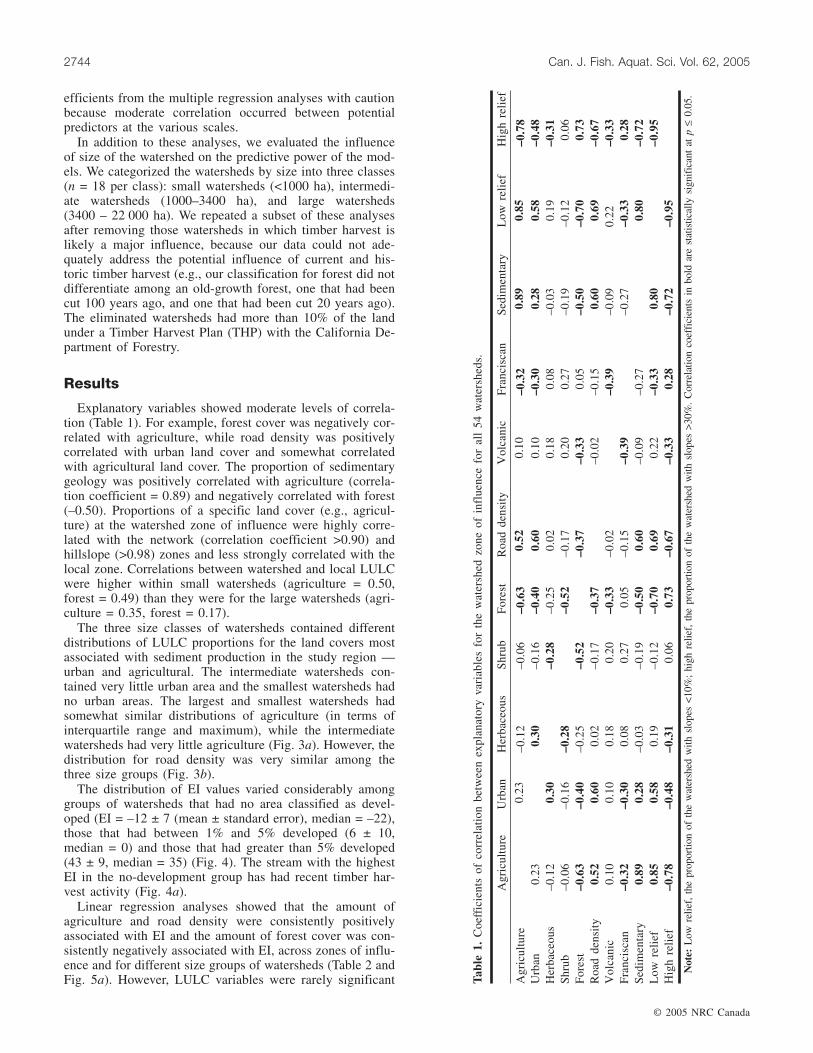
Explanatory variables showed moderate levels of correla-tion (Table 1). For example, forest cover was negatively cor-related with agriculture, while road density was positivelycorrelated with urban land cover and somewhat correlatedwith agricultural land cover. The proportion of sedimentarygeology was positively correlated with agriculture (correla-tion coefficient = 0.89) and negatively correlated with forest(–0.50). Proportions of a specific land cover (e.g., agricul-ture) at the watershed zone of influence were highly corre-lated with the network (correlation coefficient >0.90) andhillslope (>0.98) zones and less strongly correlated with thelocal zone. Correlations between watershed and local LULCwere higher within small watersheds (agriculture = 0.50,forest = 0.49) than they were for the large watersheds (agri-culture = 0.35, forest = 0.17).

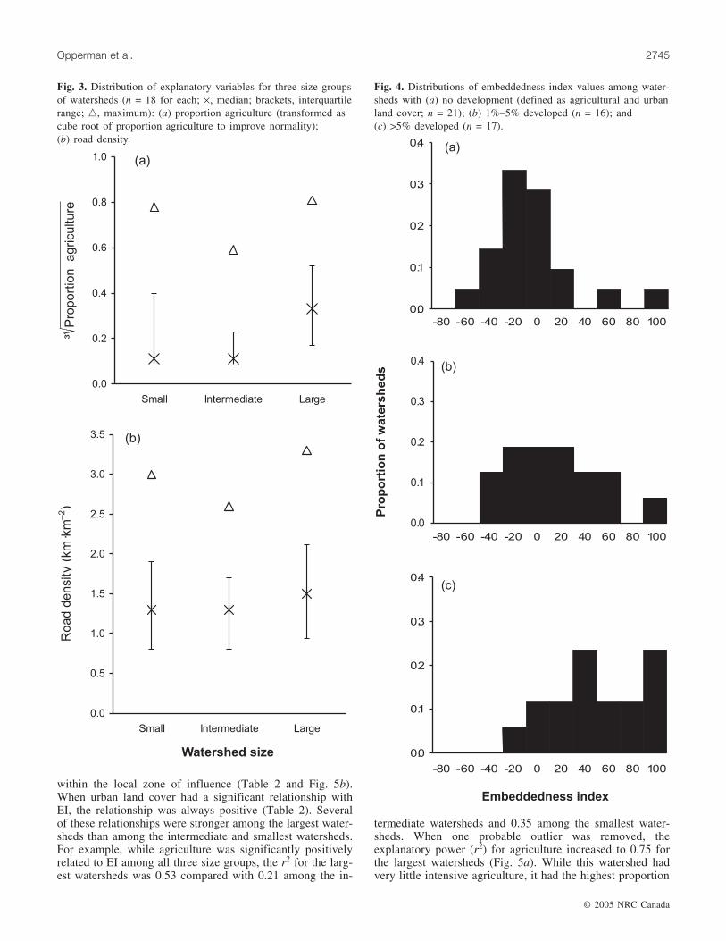
The three size classes of watersheds contained differentdistributions of LULC proportions for the land covers mostassociated with sediment production in the study region —urban and agricultural. The intermediate watersheds con-tained very little urban area and the smallest watersheds hadno urban areas. The largest and smallest watersheds hadsomewhat similar distributions of agriculture (in terms ofinterquartile range and maximum), while the intermediatewatersheds had very little agriculture (Fig. 3a). However, thedistribution for road density was very similar among thethree size groups (Fig. 3b).

The distribution of EI values varied considerably amonggroups of watersheds that had no area classified as devel-oped (EI = –12 ± 7 (mean ± standard error), median = –22),those that had between 1% and 5% developed (6 ± 10,median = 0) and those that had greater than 5% developed(43 ± 9, median = 35) (Fig. 4). The stream with the highestEI in the no-development group has had recent timber har-vest activity (Fig. 4a).

Linear regression analyses showed that the amount ofagriculture and road density were consistently positivelyassociated with EI and the amount of forest cover was con-sistently negatively associated with EI, across zones of influ-ence and for different size groups of watersheds (Table 2 andFig. 5a). However, LULC variables were rarely significant

© 2005 NRC Canada

2744 Can. J. Fish. Aquat. Sci. Vol. 62, 2005

Agr

icul

ture

Urb

anH

erba

ceou

sS

hrub

For

est

Roa

dde

nsit

yV

olca

nic

Fra

ncis

can

Sed

imen

tary

Low

reli

efH

igh

reli

ef

Agr

icul

ture

0.23

–0.1

2–0

.06

–0.6

30.

520.

10–0

.32

0.89

0.85

–0.7

8U

rban

0.23

0.30

–0.1

6–0

.40

0.60

0.10

–0.3

00.

280.

58–0

.48

Her

bace

ous

–0.1

20.

30–0

.28

–0.2

50.

020.

180.

08–0

.03

0.19

–0.3

1S

hrub

–0.0

6–0

.16

–0.2

8–0

.52

–0.1

70.

200.

27–0

.19

–0.1

20.

06F

ores

t–0

.63

–0.4

0–0

.25

–0.5

2–0

.37

–0.3

30.

05–0

.50

–0.7

00.

73R

oad

dens

ity

0.52

0.60

0.02

–0.1

7–0

.37

–0.0

2–0

.15

0.60

0.69

–0.6

7V

olca

nic

0.10

0.10

0.18

0.20

–0.3

3–0

.02

–0.3

9–0

.09

0.22

–0.3

3F

ranc

isca

n–0

.32

–0.3

00.

080.

270.

05–0

.15

–0.3

9–0

.27

–0.3

30.

28S

edim

enta

ry0.

890.

28–0

.03

–0.1

9–0

.50

0.60

–0.0

9–0

.27

0.80

–0.7

2L

owre

lief

0.85

0.58

0.19

–0.1

2–0

.70

0.69

0.22

–0.3

30.

80–0

.95

Hig

hre

lief

–0.7

8–0

.48

–0.3

10.

060.

73–0

.67

–0.3

30.

28–0

.72

–0.9

5

Not

e:L

owre

lief,

the

prop

ortio

nof

the

wat

ersh

edw

ithsl

opes

<10%

;hi

ghre

lief,

the

prop

ortio

nof

the

wat

ersh

edw

ithsl

opes

>30%

.C

orre

latio

nco

effi

cien

tsin

bold

are

stat

istic

ally

sign

ific

ant

atp

≤0.

05.

Tab

le1.

Coe

ffic

ient

sof

corr

elat

ion

betw

een

expl

anat

ory

vari

able

sfo

rth

ew

ater

shed

zone

ofin

flue

nce

for

all

54w

ater

shed

s.

within the local zone of influence (Table 2 and Fig. 5b).When urban land cover had a significant relationship withEI, the relationship was always positive (Table 2). Severalof these relationships were stronger among the largest water-sheds than among the intermediate and smallest watersheds.For example, while agriculture was significantly positivelyrelated to EI among all three size groups, the r2 for the larg-est watersheds was 0.53 compared with 0.21 among the in-

termediate watersheds and 0.35 among the smallest water-sheds. When one probable outlier was removed, theexplanatory power (r2) for agriculture increased to 0.75 forthe largest watersheds (Fig. 5a). While this watershed hadvery little intensive agriculture, it had the highest proportion

© 2005 NRC Canada

Opperman et al. 2745

Fig. 3. Distribution of explanatory variables for three size groupsof watersheds (n = 18 for each; ×, median; brackets, interquartilerange; �, maximum): (a) proportion agriculture (transformed ascube root of proportion agriculture to improve normality);(b) road density.

Fig. 4. Distributions of embeddedness index values among water-sheds with (a) no development (defined as agricultural and urbanland cover; n = 21); (b) 1%–5% developed (n = 16); and(c) >5% developed (n = 17).

urban and highest road density of all 54 watersheds. For themost part, geological variables were not correlated with EI.However, the proportion of sedimentary geology was posi-tively and significantly correlated with EI for the watershed,hillslope, and network zones of influence.

Comparing the multiple regression models for each zoneof influence for the full set of 54 reaches, the model for wa-tershed had the greatest explanatory power (radj

2 0.42= ), fol-lowed by network (radj

2 0.32= ) and hillslope (radj2 0.29= ;

Fig. 6). The local zone of influence had the lowest explana-tory power (radj

2 0.07= ). Geological variables were not se-lected within the multiple regression models. Stepwiseregression consistently selected proportion agriculture as asignificant model term, with a positive relationship with EI,for all zones of influence with the exception of local.

The size of the watershed influenced the predictive powerof the empirical models, with explanatory power decreasingfrom larger to smaller watersheds (Fig. 6). The largest water-sheds displayed trends similar to those for all watershedscombined, with the watershed zone having the greatest ex-planatory power (radj

2 0.73= ), followed closely by network(radj

2 0.70= ) and hillslope (radj2 0.65= ). The upstream zone

had much lower explanatory power, and the local zone hadalmost no explanatory power. Within these models, terms foragriculture, road density, urban, and herbaceous had positiverelationships with EI, while forest and shrub had negative re-lationships with EI.

The smallest watersheds displayed a different trend, withthe upstream zone having the greatest explanatory power(radj

2 0.46= ), followed by network (radj2 0.38= ); local, water-

shed, and hillslope zones had relatively low explanatorypower (radj

2 ranging from 0.22 to 0.34; Fig. 6). Proportion ag-riculture was also selected as a significant model term, witha positive relationship with EI, for all zones of influence.Intermediate watersheds had very little spread in LULC dis-tributions for urban and agriculture (Fig. 3a). Explanatory

power (i.e., adjusted r2) for all zones of influence was gener-ally lower than either the smallest or largest watersheds(Fig. 6).

Repeating the watershed zone analyses after removingwatersheds with >10% THP somewhat strengthened the ex-planatory power for the overall set of watersheds (n = 39)and the largest watersheds (n = 14) but did not change theexplanatory power for the smallest watersheds (n = 14). Thetwo methods of summarizing embeddedness from the CDFGdata (the EI and the weighted average) were highly corre-lated (correlation coefficient = 0.97). The analyses conductedwith the weighted average as the response variable had es-sentially identical results in terms of explanatory power,model terms, and coefficients.

Discussion

LULC variables were effective predictors of the levels ofembeddedness of spawning substrate in streams within theRussian River Basin. Considering all 54 watersheds, LULChad the greatest explanatory power within the watershed,network, and hillslope zones of influence, with less explana-tory power for the local and upstream zones. However, water-shed size appears to have some influence on the relativestrengths of these relationships. The strongest overall rela-tionships between LULC and embeddedness were foundamong the largest watersheds at the watershed, network, andhillslope zones (with r2 between 0.65 and 0.73). Conversely,among the largest watersheds, the local zone had essentiallyno explanatory power. The next strongest relationships be-tween LULC and EI were found among the smallest water-sheds at the network and upstream scales. The intermediatewatersheds had very low levels of LULC classes generallyassociated with sediment production in the study region (ag-riculture and urban), and explanatory power for analyses

© 2005 NRC Canada

2746 Can. J. Fish. Aquat. Sci. Vol. 62, 2005

Watershedcoefficient r2

Localcoefficient r2

Upstreamcoefficient r2

Networkcoefficient r2

Hillslopecoefficient r2

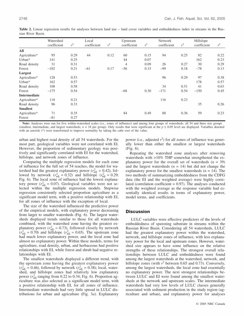
AllAgriculture* 95 0.29 44 0.12 60 0.15 94 0.25 82 0.22Urban* 141 0.25 44 0.07 162 0.23Road density 31 0.31 4 0.09 26 0.27 30 0.29Forest –102 0.21 –61 0.17 –56 0.15 –99 0.18 –78 0.13LargestAgriculture* 128 0.53 96 0.29 97 0.38Urban* 162 0.57 178 0.57Road density 108 0.58 34 0.51 41 0.63Forest –175 0.54 –68 0.30 –171 0.54 –150 0.45IntermediateAgriculture* 118 0.21 116 0.23Road density 96 0.33 35 0.26SmallestAgriculture* 71 0.35 84 0.49 88 0.36 59 0.23Forest –81 0.27

Note: Analyses were run for five within-watershed scales (i.e., zones of influence) and among four groups of watersheds: all 54 and three size groups(smallest, intermediate, and largest watersheds; n = 18 per group). Only results that were significant at the p ≤ 0.05 level are displayed. Variables denotedwith an asterisk (*) were transformed to improve normality by taking the cube root of the value.

Table 2. Linear regression results for analyses between land use – land cover variables and embeddedness index in streams in the Rus-sian River Basin.

among these watersheds was generally lower than that foreither the largest or smallest watersheds.

Results from our analyses showed that across multiplemodels and scales, LULC categories for agriculture, urban,and road density were highly significant model terms, ex-plained the most variation in EI, and were consistently posi-

tively correlated with embeddedness, while forest cover wasalways negatively correlated. Agriculture can lead to signifi-cantly higher rates of sediment production, even on moder-ate slopes, because of the increased amount of bare soilexposed to the erosive power of raindrops and sheet wash(Dunne and Leopold 1978; Chang et al. 1982; Pimentel andKounang 1998). Agriculture can also lead to higher rates ofrunoff (Chang et al. 1982), which can then increase sedi-ment load through incision and bank erosion (Kuhnle et al.1998). Similarly, urban land cover can increase peak runoffand, consequently, channel erosion (Trimble 1997; Pizzutoet al. 2000), in addition to the large amounts of fine sedi-ment produced during periods of construction (Dunne andLeopold 1978). Numerous studies have linked roads with theproduction of sediment, particularly in areas with rugged to-pography (Swanson and Dyrness 1975; Montgomery 1994;Jones et al. 2000).

Our results suggest that increased sediment produced di-rectly or indirectly from agricultural and urban areas androads may be one mechanism by which these land usesdegrade stream habitat and potentially influence salmonidabundance and recovery. In a study relating fish abundancewith watershed characteristics, Bradford and Irvine (2000)reported that agricultural land use was associated with de-clines in coho salmon populations within 40 tributary water-sheds of the Thompson River, British Columbia. Similarly,Pess et al. (2002) showed that coho salmon abundance in theSnohomish Basin in Washington was negatively correlatedwith the percentage of watershed in agriculture, urban devel-opment, and roads. The abundance of juvenile chinooksalmon was also negatively correlated with road density in astudy in Idaho (Thompson and Lee 2000). Sutherland et al.(2002) reported that increased fine sediment from disturbedwatersheds in the southern Appalachians altered stream fish

© 2005 NRC Canada

Opperman et al. 2747

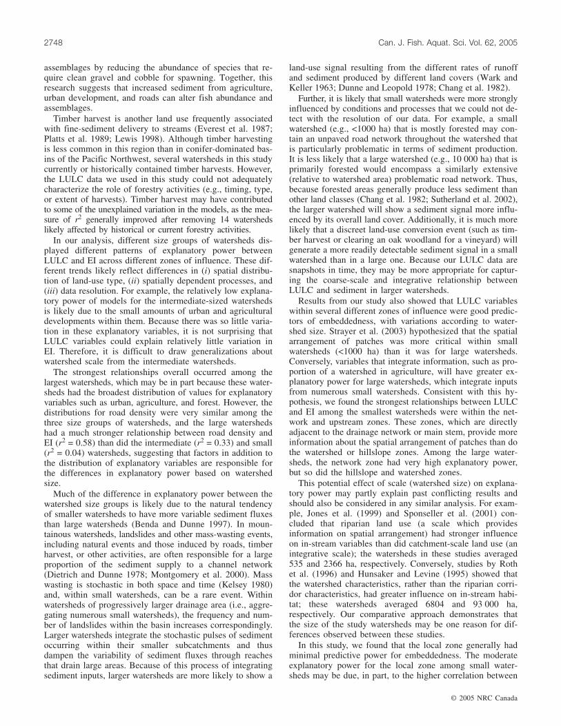
Fig. 5. (a) The embeddedness index plotted against the propor-tion of watershed in agriculture for the 18 largest watersheds; thearrow indicates a watershed that is less than 33% forested with18% urban and the highest road density of the 54 watersheds.(b) The embeddedness index plotted against the proportion of thelocal riparian corridor in agriculture for the 18 largest water-sheds. The proportion of agriculture in both zones of influencewas transformed as a cube root to improve normality.

Fig. 6. Explanatory power (radj2 ) of models focused on five zones

of influence for four samples of watersheds: all 54 watersheds(solid bars), smallest (open bars), intermediate (darker shadedbars), and largest (lighter shaded bars) watersheds. The line re-flects the proportion of the watershed’s total area that is encom-passed within a given zone of influence (median ± 25th and 75thpercentiles (brackets)).

assemblages by reducing the abundance of species that re-quire clean gravel and cobble for spawning. Together, thisresearch suggests that increased sediment from agriculture,urban development, and roads can alter fish abundance andassemblages.

Timber harvest is another land use frequently associatedwith fine-sediment delivery to streams (Everest et al. 1987;Platts et al. 1989; Lewis 1998). Although timber harvestingis less common in this region than in conifer-dominated bas-ins of the Pacific Northwest, several watersheds in this studycurrently or historically contained timber harvests. However,the LULC data we used in this study could not adequatelycharacterize the role of forestry activities (e.g., timing, type,or extent of harvests). Timber harvest may have contributedto some of the unexplained variation in the models, as the mea-sure of r2 generally improved after removing 14 watershedslikely affected by historical or current forestry activities.

In our analysis, different size groups of watersheds dis-played different patterns of explanatory power betweenLULC and EI across different zones of influence. These dif-ferent trends likely reflect differences in (i) spatial distribu-tion of land-use type, (ii) spatially dependent processes, and(iii) data resolution. For example, the relatively low explana-tory power of models for the intermediate-sized watershedsis likely due to the small amounts of urban and agriculturaldevelopments within them. Because there was so little varia-tion in these explanatory variables, it is not surprising thatLULC variables could explain relatively little variation inEI. Therefore, it is difficult to draw generalizations aboutwatershed scale from the intermediate watersheds.

The strongest relationships overall occurred among thelargest watersheds, which may be in part because these water-sheds had the broadest distribution of values for explanatoryvariables such as urban, agriculture, and forest. However, thedistributions for road density were very similar among thethree size groups of watersheds, and the large watershedshad a much stronger relationship between road density andEI (r2 = 0.58) than did the intermediate (r2 = 0.33) and small(r2 = 0.04) watersheds, suggesting that factors in addition tothe distribution of explanatory variables are responsible forthe differences in explanatory power based on watershedsize.

Much of the difference in explanatory power between thewatershed size groups is likely due to the natural tendencyof smaller watersheds to have more variable sediment fluxesthan large watersheds (Benda and Dunne 1997). In moun-tainous watersheds, landslides and other mass-wasting events,including natural events and those induced by roads, timberharvest, or other activities, are often responsible for a largeproportion of the sediment supply to a channel network(Dietrich and Dunne 1978; Montgomery et al. 2000). Masswasting is stochastic in both space and time (Kelsey 1980)and, within small watersheds, can be a rare event. Withinwatersheds of progressively larger drainage area (i.e., aggre-gating numerous small watersheds), the frequency and num-ber of landslides within the basin increases correspondingly.Larger watersheds integrate the stochastic pulses of sedimentoccurring within their smaller subcatchments and thusdampen the variability of sediment fluxes through reachesthat drain large areas. Because of this process of integratingsediment inputs, larger watersheds are more likely to show a

land-use signal resulting from the different rates of runoffand sediment produced by different land covers (Wark andKeller 1963; Dunne and Leopold 1978; Chang et al. 1982).

Further, it is likely that small watersheds were more stronglyinfluenced by conditions and processes that we could not de-tect with the resolution of our data. For example, a smallwatershed (e.g., <1000 ha) that is mostly forested may con-tain an unpaved road network throughout the watershed thatis particularly problematic in terms of sediment production.It is less likely that a large watershed (e.g., 10 000 ha) that isprimarily forested would encompass a similarly extensive(relative to watershed area) problematic road network. Thus,because forested areas generally produce less sediment thanother land classes (Chang et al. 1982; Sutherland et al. 2002),the larger watershed will show a sediment signal more influ-enced by its overall land cover. Additionally, it is much morelikely that a discreet land-use conversion event (such as tim-ber harvest or clearing an oak woodland for a vineyard) willgenerate a more readily detectable sediment signal in a smallwatershed than in a large one. Because our LULC data aresnapshots in time, they may be more appropriate for captur-ing the coarse-scale and integrative relationship betweenLULC and sediment in larger watersheds.

Results from our study also showed that LULC variableswithin several different zones of influence were good predic-tors of embeddedness, with variations according to water-shed size. Strayer et al. (2003) hypothesized that the spatialarrangement of patches was more critical within smallwatersheds (<1000 ha) than it was for large watersheds.Conversely, variables that integrate information, such as pro-portion of a watershed in agriculture, will have greater ex-planatory power for large watersheds, which integrate inputsfrom numerous small watersheds. Consistent with this hy-pothesis, we found the strongest relationships between LULCand EI among the smallest watersheds were within the net-work and upstream zones. These zones, which are directlyadjacent to the drainage network or main stem, provide moreinformation about the spatial arrangement of patches than dothe watershed or hillslope zones. Among the large water-sheds, the network zone had very high explanatory power,but so did the hillslope and watershed zones.

This potential effect of scale (watershed size) on explana-tory power may partly explain past conflicting results andshould also be considered in any similar analysis. For exam-ple, Jones et al. (1999) and Sponseller et al. (2001) con-cluded that riparian land use (a scale which providesinformation on spatial arrangement) had stronger influenceon in-stream variables than did catchment-scale land use (anintegrative scale); the watersheds in these studies averaged535 and 2366 ha, respectively. Conversely, studies by Rothet al. (1996) and Hunsaker and Levine (1995) showed thatthe watershed characteristics, rather than the riparian corri-dor characteristics, had greater influence on in-stream habi-tat; these watersheds averaged 6804 and 93 000 ha,respectively. Our comparative approach demonstrates thatthe size of the study watersheds may be one reason for dif-ferences observed between these studies.

In this study, we found that the local zone generally hadminimal predictive power for embeddedness. The moderateexplanatory power for the local zone among small water-sheds may be due, in part, to the higher correlation between

© 2005 NRC Canada

2748 Can. J. Fish. Aquat. Sci. Vol. 62, 2005

LULC classes (e.g., forest and agriculture) at the local andwatershed zones for small watersheds than for large water-sheds. The general lack of influence of the local zone is notsurprising, given that it represents a very small proportion ofthe total watershed and the surveyed reaches are receivingrunoff from hundreds to thousands of hectares. Because ri-parian land cover had little relationship to embeddedness, itis unlikely that reach-scale riparian restoration will improvespawning conditions within the lower reaches of watershedsif conditions within the rest of the watershed remain un-changed. However, we do want to note that it is difficult todetermine which zone of influence has the strongest predic-tive power for embeddedness, in large part because LULC inthe zones of watershed, hillslope, and network are so highlycorrelated.

Because the LULC variables were derived from one mo-ment in time, this analysis cannot account for the timing ofland-use conversion or capture the legacies of historical landuse, which can continue to exert influences on streams fordecades (Harding et al. 1998). Historical legacies and thetiming of conversions are undoubtedly responsible for a largeportion of the unexplained variation in the models. Studies,such as this one, that examine relationships between currentland-use patterns and in-stream variables must be cautious tonot infer causation from correlation. For example, we do notknow the distribution of embeddedness values within Rus-sian River watersheds prior to any anthropogenic changes inland cover. However, comparing the distributions of EIwithin watersheds with no development with those morethan 5% developed provides strong support for the role ofanthropogenic land-cover conversion in increasing sedimentlevels in Russian River tributary streams. Although thisstudy’s approach cannot explain the mechanisms by whichthis happened, the mechanisms by which changes in landcover increase sediment production are well established atsmaller scales (e.g., plots, small experimental watersheds)(Dunne and Leopold 1978; Chang and Tsai 1991; Battanyand Grismer 2000). Combining empirical approaches withfuture mechanistic research (both experimental and model-ing) will further improve our understanding of the linkagesbetween land use and in-stream habitat (Strayer et al. 2003).

Our data are the first to relate patterns of fine sediments instreams to patterns of land use in Mediterranean-climate wa-tersheds in California, and these data suggest that agricul-tural land use is correlated with elevated levels of finesediment. Over the past decade, vineyards in the RussianRiver and Napa River basins have expanded onto hillslopesbecause of limited land availability in valley bottoms(Merenlender 2000). A recent study projects that 80% of fu-ture vineyards in Napa County will be planted on hillslopes(Napa County RCD 1997). Hillside vineyards in this regioncan produce annual soil loss ranging from 5 to 50 t·ha–1

(Battany and Grismer 2000). Battany and Grismer (2000),working in Napa County, found that soil cover was the pri-mary factor affecting erosion rates from hillslope vineyards,with slope as a secondary factor. This observation empha-sizes the potentially important role that management prac-tices can play in reducing the impacts from agricultural landuse.

In conclusion, the results of our study suggest thatwatershed-scale patterns of land use, including both the land

adjacent to the entire upstream channel network and the sur-rounding hillslopes, are generally the best predictors ofstream sediment conditions. Local land cover (i.e., the adja-cent riparian corridor) had little relationship to embedded-ness. Much attention and resources have been spent onpiecemeal stream restoration and sediment control efforts atthe local scale (e.g., bank stabilization). Our data indicatethat the effects of such localized efforts will be over-whelmed by processes operating at larger scales and, thus,have little influence on spawning conditions. Rather, toimprove spawning gravels, restoration efforts should empha-size protecting riparian corridors throughout entire water-sheds and promote programs or policies that ameliorate theinfluences of roads and agricultural land use. However, evenwatersheds with relatively low levels of development (e.g.,5% of a watershed) had relatively high embeddedness scores,suggesting a limit to the improvements that restoration pro-grams can hope to achieve. The landscape-scale approach ofthis study emphasizes the overarching importance of large-scale land-use patterns. With such an approach, managersand policy-makers can identify priority areas for protectionand restoration and, when combined with projections of fu-ture land-use change, identify particularly vulnerable water-sheds.

Acknowledgements

This research was funded by the University of California’sWater Resources Center and the California Department ofFish and Game. We thank Robert Coey, Barry Collins, andDerek Acomb for the habitat data and continued support ofour research efforts and G.M. Kondolf for input on an earlierversion of this paper.

References

Allan, J.D., and Johnson, L.B. 1997. Catchment-scale analysis ofaquatic ecosystems. Freshw. Biol. 37: 107–111.

Allan, J.D., Erickson, D.L., and Fay, J. 1997. The influence ofcatchment land use on stream integrity across multiple spatialscales. Freshw. Biol. 37: 149–161.

Battany, M.C., and Grismer, M.E. 2000. Rainfall runoff and ero-sion in Napa Valley vineyards: effects of slope, cover and sur-face roughness. Hydrol. Process. 14: 1289–1304.

Benda, L., and Dunne, T. 1997. Stochastic forcing of sediment sup-ply to channel networks from landsliding and debris flows. Wa-ter Resour. Res. 33: 2849–2863.

Bradford, M.J., and Irvine, J.R. 2000. Land use, fishing, climatechange, and the decline of Thompson River, British Columbia,coho salmon. Can. J. Fish. Aquat. Sci. 57: 13–16.

Busby, P.J., Wainwright, T.C., and Bryant, G.J. 2000. Status reviewof steelhead from Washington, Idaho, Oregon, and California. InSustainable fisheries management: Pacific salmon. Edited byE.E. Knudsen, C.R. Steward, D.D. MacDonal, J.E. Williams,and D.W. Reiser. Lewis Publishers, New York. pp. 119–132.

Chang, K., and Tsai, B. 1991. The effect of DEM resolution onslope and aspect mapping. Cartogr. Geogr. Inform. 18: 69–77.

Chang, M., Roth, F.A., and Hunt, E.V. 1982. Sediment productionunder various forest-site conditions. In Recent developments inthe explanation and prediction of erosion and sediment yield. Int.Assoc. Hydrol. Sci. Publ. No. 137, Wallingford, UK. pp. 13–22.

© 2005 NRC Canada

Opperman et al. 2749

Dietrich, W.E., and Dunne, T. 1978. Sediment budget for a smallcatchment in mountainous terrain. Z. Geomorphol. 29(Suppl.):191–206.

Dunne, T., and Leopold, L.B. 1978. Water in environmental plan-ning. W.H. Freeman and Company, New York.

Everest, F.H., Beschta, R.L., Scrivener, J.C., Koski, K.V., Sedell,J.R., and Cederholm, C.J. 1987. Fine sediment and salmonidproduction: a paradox. In Streamside management: forestry andfisheries interactions. Edited by E.O. Salo and T.W. Cundy. Uni-versity of Washington Press, Seattle, Wash. pp. 98–142.

Gasith, A., and Resh, V.H. 1999. Streams in Mediterranean climateregions: abiotic influences and biotic responses to predictableseasonal events. Annu. Rev. Ecol. Syst. 30: 51–81.

Hansen, W.F. 2001. Identifying stream types and management im-plications. For. Ecol. Manag. 143: 39–46.

Harding, J.S., Benfield, E.F., Bolstad, P.V., Helfman, G.S., andJones, E.B.D.I. 1998. Stream biodiversity: the ghost of land usepast. Proc. Natl. Acad. Sci. U.S.A. 95: 14 843–14 847.

Heaton, E., and Merenlender, A.M. 2000. Modeling vineyard expan-sion, potential habitat fragmentation. Calif. Agric. 54: 12–19.

Henley, W.F., Patterson, M.A., Neves, R.J., and Lemly, A.D. 2000.Effects of sedimentation and turbidity on lotic food webs: a con-cise review for natural resource managers. Rev. Fish. Sci. 8:125–139.

Hunsaker, C.T., and Levine, D.A. 1995. Hierarchical approaches tothe study of water quality in rivers. Bioscience, 45: 193–203.

Jones, E.B.D.I., Helfman, G.S., Harper, J.O., and Bolstad, P.V.1999. Effects of riparian forest removal on fish assemblages insouthern Appalachian streams. Conserv. Biol. 13: 1454–1465.

Jones, J.A., Swanson, F.J., Wemple, B.C., and Snyder, K.U. 2000.Effects of roads on hydrology, geomorphology, and disturbancepatches in stream networks. Conserv. Biol. 14: 76–85.

Kelsey, H.M. 1980. A sediment budget and an analysis of geomorphicprocess in the Van Duzen River basin, north coastal California.Geol. Soc. Am. Bull. 91: 190–195.

Kondolf, G.M. 2000. Assessing salmonid spawning gravel quality.Trans. Am. Fish. Soc. 129: 262–281.

Kuhnle, R.A., Bingner, R.L., Foster, G.R., and Grissinger, E.H. 1998.Land use change and sediment transport in Goodwin Creek. InGravel-bed rivers in the environment. Edited by P.C. Klingeman,R.L. Beschta, P.D. Komar, and J.B. Bradley. Water Resources Pub-lications, LLC, Highlands Ranch, Co. pp. 279–292.

Lammert, M., and Allan, J.D. 1999. Assessing biotic integrity ofstreams: effects of scale in measuring the influence of landuse/cover and habitat structure on fish and macroinvertebrates.Environ. Manag. 23: 257–270.

Lewis, J. 1998. Evaluating the impacts of logging activities on ero-sion and suspended sediment transport in the Caspar Creek water-sheds. In Proceedings of the conference on coastal watersheds:the Caspar Creek story. Edited by R.R. Ziemer. Pacific SouthwestResearch Station, Forest Service, US Department of Agriculture,Ukiah, Calif. pp. 55–69.

McIntosh, B.A., Sedell, J.R., Thurow, R.F., Clarke, S.E., and Chan-dler, G.L. 2000. Historical changes in pool habitats in the Co-lumbia River Basin. Ecol. Appl. 10: 1478–1496.

Merenlender, A.M. 2000. Mapping vineyard expansion providesinformation on agriculture and the environment. Calif. Agric.54: 7–12.

Merenlender, A.M., Heise, K.L., and Brooks, C. 1998. Effects ofsubdividing private property on biodiversity in California’s northcoast oak woodlands. Trans. W. Sect. Wild. Soc. 34: 9–20.

Mills, T.J., McEwan, D., and Jennings, M.R. 1997. California salmonand steelhead: beyond the crossroads. In Pacific salmon and theirecosystems: status and future options. Edited by D.J. Stouder, P.A.

Bisson, R.J. Naiman, and M.G. Duke. Chapman & Hall, NewYork. pp. 91–112.

Montgomery, D.R. 1994. Road surface drainage, channel initiation,and slope instability. Water Resour. Res. 30: 1925–1932.

Montgomery, D.R., and Buffington, J.M. 1993. Channel classifica-tion, prediction of channel response, and assessment of channelcondition. Washington Department of Natural Resources Rep.No. TFW-SH10-93-002.

Montgomery, D.R., and Dietrich, W.E. 1988. Where do channelsbegin? Nature (Lond.), 336: 232–234.

Montgomery, D.R., Schmidt, K.M., Greenberg, H.M., and Dietrich,W.E. 2000. Forest clearing and regional landsliding. Geology,28: 311–314.

Moyle, P.B. 2002. Inland fishes of California. University of Cali-fornia Press, Berkeley, Calif.

Napa County Resource Conservation District (RCD). 1997. NapaRiver watershed owner’s manual. Napa County Resource Con-servation District, Napa, Calif.

National Research Council. 1996. Upstream: salmon and society inthe Pacific Northwest. National Academy Press, Washington, D.C.

Nehlsen, W. 1997. Pacific salmon status and trends — a coastwideperspective. In Pacific salmon and their ecosystems: status andfuture options. Edited by D.J. Stouder, P.A. Bisson, R.J. Naiman,and M.G. Duke. Chapman & Hall, New York. pp. 41–52.

Nehlsen, W., Williams, J.E., and Lichatowich, J.A. 1991. Pacificsalmon at the crossroads: stocks at risk in California, Oregon,Idaho and Washington. Fisheries, 16: 4–21.

Nilsson, C., Pizzuto, J.E., Moglen, G.E., Palmer, M.A., Stanley, E.H.,Bockstael, N.E., and Thompson, L.C. 2003. Ecological forecastingand the urbanization of stream ecosystems: challenges for econo-mists, hydrologists, geomorphologists, and ecologists. Ecosystems,6: 659–674.

Omernik, J.M., Abernathy, A.R., and Male, L.M. 1981. Stream nutri-ent levels and proximity of agricultural and forest land to streams:some relationships. J. Soil Water Conserv. 36: 227–231.

Paulsen, C.M., and Fisher, T.R. 2001. Statistical relationship be-tween parr-to-smolt survival of Snake River spring–summer Chi-nook salmon and indices of land use. Trans. Am. Fish. Soc. 130:347–358.

Pess, G.R., Montgomery, D.R., Steel, E.A., Bilby, R.E., Feist, B.E.,and Greenberg, H.M. 2002. Landscape characteristics, land use,and coho salmon (Oncorhynchus kisutch) abundance, SnohomishRiver, Wash., U.S.A. Can. J. Fish. Aquat. Sci. 59: 613–623.

Pimentel, D., and Kounang, N. 1998. Ecology of soil erosion inecosystems. Ecosystems, 1: 416–426.

Pizzuto, J.E., Hession, W.C., and McBride, M. 2000. Comparinggravel-bed rivers in paired urban and rural catchments of south-eastern Pennsylvania. Geology, 28: 79–82.

Platts, W.S., Torquemada, R.J., McHenry, M.L., and Graham, C.K.1989. Changes in salmonid spawning and rearing habitat fromincreased delivery of fine sediment to the South Fork SalmonRiver, Idaho. Trans. Am. Fish. Soc. 118: 274–283.

Radko, M.A. 1997. Spatially linking basinwide stream inventoriesto arcs representing streams in a Geographic Information Sys-tem. USDA Forest Service Rep. INT-GTR-345.

Regetz, J. 2003. Landscape-level constraints on recruitment of chi-nook salmon (Oncorhynchus tshawytscha) in the Columbia RiverBasin, U.S.A. Aquat. Conserv. 13: 35–49.

Reiser, D.W., and White, R.G. 1988. Effects of two sediment size-classes on survival of steelhead and chinook salmon eggs. N.Am. J. Fish. Manag. 8: 432 – 437.

Richards, C., Johnson, L.B., and Host, G.E. 1996. Landscape-scaleinfluences on stream habitats and biota. Can. J. Fish. Aquat. Sci.53: 295–311.

© 2005 NRC Canada

2750 Can. J. Fish. Aquat. Sci. Vol. 62, 2005

Roni, P., Beechie, T.J., Bilby, R.E., Leonetti, F.E., Pollock, M.M.,and Pess, G.R. 2002. A review of stream restoration techniquesand a hierarchical strategy for prioritizing restoration in PacificNorthwest watersheds. N. Am. J. Fish. Manag. 22: 1–20.

Roper, B.D., Dose, J.J., and Williams, J.E. 1997. Stream restora-tion: is fisheries biology enough? Fisheries, 22: 6–11.

Roth, N.E., Allan, J.D., and Erickson, D.L. 1996. Landscape influ-ences on stream biotic integrity assessed at multiple spatial scales.Landsc. Ecol. 11: 141–156.

Snyder, C.D., Young, J.A., Villella, R., and Lemarie, D.P. 2003. In-fluences of upland and riparian land use patterns on stream bi-otic integrity. Landsc. Ecol. 18: 647–664.

Sponseller, R.A., Benfield, E.F., and Valett, H.M. 2001. Relationshipsbetween land use, spatial scale and stream macroinvertebrate com-munities. Freshw. Biol. 46: 1409–1424.

Strayer, D.L., Beighley, R.E., Thompson, L.C., Brooks, S., Nilsson,C., Pinay, G., and Naiman, R.J. 2003. Effects of land-cover onstream ecosystems: roles of empirical models and scaling issues.Ecosystems, 6: 407–423.

Sutherland, A.B., Meyer, J.L., and Gardiner, E.P. 2002. Effects ofland cover on sediment regime and fish assemblage structure infour southern Appalachian streams. Freshw. Biol. 47: 1791–1805.

Suttle, K.B., Power, M.E., Levine, J.M., and McNeely, C. 2004.How fine sediment in riverbeds impairs growth and survival ofjuvenile salmonids. Ecol. Appl. 14: 2004.

Swanson, F.J., and Dyrness, C.T. 1975. Impact of clear-cutting androad construction on soil erosion by landslides in the westernCascade Range, Oregon. Geology, 3: 393–396.

Thompson, W.L., and Lee, D.C. 2000. Modeling relationships be-tween landscape-level attributes and snorkel counts of chinooksalmon and steelhead parr in Idaho. Can. J. Fish. Aquat. Sci. 57:1834–1842.

Trimble, S.W. 1997. Contribution of stream channel erosion to sedi-ment yield from an urbanizing watershed. Science (Wash., D.C.),278: 1442–1444.

Wang, L., Lyons, J., Kanehl, P., and Gatti, R. 1997. Influences ofwatershed land use on habitat quality and biotic integrity in Wis-consin streams. Fisheries, 22: 6–12.

Wark, J.W., and Keller, F.J. 1963. Preliminary study of sedimentsources and transport in the Potomac River Basin. InterstateCommission on the Potomac River Basin, Edgewater, Md.

Waters, T.F. 1995. Sediment in streams: sources, biological effectsand control. Am. Fish. Soc. Monogr. No. 7, Bethesda, Md.

Weitkamp, L., Wainwright, T.C., Bryant, G.J., Teel, D.J., and Kope,R.G. 2000. Review of the status of coho salmon from Washing-ton, Oregon, and California. In Sustainable fisheries management:Pacific salmon. Edited by E.E. Knudsen, C.R. Steward, D.D.MacDonal, J.E. Williams, and D.W. Reiser. Lewis Publishers,New York. pp. 111–118.

Wohl, N.E., and Carline, R.F. 1996. Relations among riparian graz-ing, sediment loads, macroinvertebrates, and fishes in three cen-tral Pennsylvania streams. Can. J. Fish. Aquat. Sci. 53(Suppl. 1):260–266.

© 2005 NRC Canada

Opperman et al. 2751