Embed Size (px)
Citation preview

AN EXAMINATION OF SEARCH ROUTINESUSED IN SLOPE STABILITY ANALYSES
Item Type text; Thesis-Reproduction (electronic)
Authors Gillett, Susan Gille, 1957-
Publisher The University of Arizona.
Rights Copyright © is held by the author. Digital access to this materialis made possible by the University Libraries, University of Arizona.Further transmission, reproduction or presentation (such aspublic display or performance) of protected items is prohibitedexcept with permission of the author.
Download date 07/06/2018 07:01:49
Link to Item http://hdl.handle.net/10150/276433

INFORMATION TO USERS
This reproduction was made from a copy of a document sent to us for microfilming. While the most advanced technology has been used to photograph and reproduce this document, the quality of the reproduction is heavily dependent upon the quality of the material submitted.
The following explanation of techniques is provided to help clarify markings or notations which may appear on this reproduction.
1.The sign or "target" for pages apparently lacking from the document photographed is "Missing Page(s)". If it was possible to obtain the missing page(s) or section, they are spliced into the film along with adjacent pages. This may have necessitated cutting through an image and duplicating adjacent pages to assure complete continuity.
2. When an image on the film is obliterated with a round black mark, it is an indication of either blurred copy because of movement during exposure, duplicate copy, or copyrighted materials that should not have been filmed. For blurred pages, a good image of the page can be found in the adjacent frame. If copyrighted materials were deleted, a target note will appear listing the pages in the adjacent frame.
3. When a map, drawing or chart, etc., is part of the material being photographed, a definite method of "sectioning" the material has been followed. It is customary to begin filming at the upper left hand corner of a large sheet and to continue from left to right in equal sections with small overlaps. If necessary, sectioning is continued again—beginning below the first row and continuing on until complete.
4. For illustrations that cannot be satisfactorily reproduced by xerographic means, photographic prints can be purchased at additional cost and inserted into your xerographic copy. These prints are available upon request from the Dissertations Customer Services Department.
5. Some pages in any document may have indistinct print. In all cases the best available copy has been filmed.
University Micnjfilms
International 300 N. Zeeb Road Ann Arbor, Mt 48106


Order Number 1330549
An examination of search routines used in slope stability analyses
Gillett, Susan Gille, M.S.
The University of Arizona, 1987
U-M-I 300 N. Zeeb RtL Ann Aibor, MI 48106


PLEASE NOTE:
In alt cases this material has been filmed in the best possible way from the available copy. Problems encountered with this document have been identified herewith a check mark V •
1. Glossy photographs or pages
2. Colored illustrations, paper or print
3. Photographs with dark background
4. Illustrations are poor copy
5. Pages with black marks, not original copy
6. Print shows through as there is text on both sides of page
7. Indistinct, broken or small print on several pages */
8. Print exceeds margin requirements
9. Tightly bound copy with print lost in spine
10. Computer printout pages with indistinct print
11. Page(s) lacking when material received, and not available from school or author.
12. Page(s) seem to be missing in numbering only as text follows.
13. Two pages numbered . Text follows.
14. Curling and wrinkled pages
15. Dissertation contains pages with print at a slant, filmed as received
16. Other
University Microfilms
International


AN EXAMINATION OF SEARCH ROUTINES
USED IN SLOPE STABILITY ANALYSES
by
Susan Gille Gillett
A Thesis Submitted to the Faculty of the
DEPARTMENT OF CIVIL ENGINEERING AND ENGINEERING HECHANICS
In Partial Fulfillment of the Requirements For the Degree of
MASTER OF SCIENCE WITH A MAJOR IN CIVIL ENGINEERING
In the Graduate College
THE UNIVERSITY OF ARIZONA
19 8 7

STATEMENT BY AUTHOR
This thesis has been submitted in partial fulfillment of requirements for an advanced degree at The University of Arizona and is deposited in the University Library to be made available to borrowers under rules of the Library.
Brief quotations from this thesis are allowable without special permission, provided that accurate acknowledgment of source is made. Requests for permission for extended quotation from or reproduction of this manuscript in whole or in part may be granted by the head of the major department or the Dean of the Graduate College when in his or her judgment the proposed use of the material is in the interests of scholarship. In all other instances, however, permission must be obtained from the author.
SIGNED:
APPROVAL BY THESIS DIRECTOR
This thesis has been approved on the date shown below:
Qm *7- \JzA ̂Dr. J. S. DeNatale
Assistant Professor of Civil Engineering and Engineering Mechanics
Date

ACKNOWLEDGMENT
The author would like to express her gratitude to
Dr. Jay S. DeNatale, who served as the advisor for this research
project. His guidance, encouragement, and friendship throughout the
preparation of this thesis are deeply appreciated. Dr. Edward A.
Nowatzki and Dr. Panos D. Kiousis also deserve thanks for their many
helpful comments and suggestions.
Very special thanks go to my husband, Paul, and our sons, Brian
and John. This work would not have been possible without their love,
patience and understanding. The support and encouragement of my
parents and brothers are also appreciated.
iii

TABLE OF CONTENTS
Page
LIST OF TABLES • v
LIST OF ILLUSTRATIONS vi
ABSTRACT viii
1. INTRODUCTION 1
2. LITERATURE RE7IEW 4
2.1 Existing Search Strategies ... 4 2.2 Available Optimization Techniques 18
3. MATERIALS AND METHODS 21
3.1 Modelling Slope Stability Problems for Optimization ..... ............ 21
3.2 Example Problems 24 3.3 The STABR Slope Stability Program 25 3.4 Criteria for Evaluating Relative Efficiency
of Search Strategies ..... 26
4. PRESENTATION AND DISCUSSION OF RESULTS 27
4.1 Steep Slope in Homogeneous Soil ............ 27 4.2 Mild Slope in Homogeneous Soil ............ 37 4.3 Slope in Stratified Soil 40
4.4 Birch Dam 52 4.5 Slope in Soil with Continuous
Variation of Strength 57 4.6 Stepped Slope in Homogeneous Soil 66 4.7 Case Histories 70 4.8 Comparison of Grid and Pattern Search Results ..... 70
5. SUMMARY, CONCLUSIONS AND RECOMMENDATIONS 72
5.1 Summary ....... 72 5.2 Conclusions 72 5.3 Recommendations for Further Study ........... 73
APPENDIX A: SINE CASE HISTORIES 74
APPENDIX B: STABR DATA FILES 83
REFERENCES 100
iv

LIST OF TABLES
Table Page
1 A Comparison of Available Stability Programs 5
2 A Comparison of the Various Classes of Optimization Techniques (After DeNatale* 1983) .... 20
3 Pattern Search Results for Example #1 ........... 35
4A Effect of Step Length Logic on Efficiency for Example #1 . . 36
4B Effect of Expertise on Efficiency for Example #1 36
5 Grid Search Results for Example #1............. 38
6 Pattern Search Results for Example #2 ........... 42
7A Effect of Step Length Logic on Efficiency for Example #2 . . 43
7B Effect of Expertise on Efficiency for Example #2 43
8 Grid Search Results for Example #2............. 44
9 Pattern Search Results for Example #3 50
10A Effect of Step Length Logic on Efficiency for Example #3 . . 51
10B Effect of Expertise on Efficiency for Example #3 51
11 Pattern Search Results for Example #4 55
12A Effect of Step Length Logic on Efficiency for Example #4 . . 56
12B Effect of Expertise on Efficiency for Example #4...... 56
13 Grid Search Results for Example #5. 62
14 Pattern Search Results for Example #5 ........... 64
15A Effect of Step Length Logic on Efficiency for Example #5 . . 65
15B Effect of Expertise on Efficiency for Example #5 65
16 Comparison of Grid and Pattern Search Results ....... 71
v
LIST OF ILLUSTRATIONS
Figure Page
1 Typical Grids for Grid Searches ...... 9
2 A Typical Three-Gr?.d Analysis ............... 10
3 Example of a Slope With Two Local Minimum Safety Factors (After Duncan and Buchignani, 1975) 12
4 The Pattern Search Method Used in STABR (After Lefebvre, 1971) 13
5 A Typical STABR Search Path ................ 15
6 Alternating Variable Search Method
(After Swann, 1972) 17
7 Slope Stability Models .................. 22
8 Example #1 - Steep Slope 28
9 Safety Factor Contour Plot for Example #1......... 29
10 Grid Sizes and Sequences Used in the Grid Searches .... 31
11 Initial Grids and Starting Points for Example #1 33
12 Example #2 - Mild Slope ............. 39
13 Initial Grids and Starting Points for Example #2 ..... 41
14 Example #3 - Stratified Soil Deposit ........... 46
15 Critical Circles for Three Different Tangent Elevations . . 47
16 Variation in Safety Factor With Depth for Example #3 . . . 48
17 Initial Grids and Starting Points for Example #3 ..... 49
18 Example #4 - Birch Dam 53
19 Initial Grids and Starting Points for Example #4 ..... 54
vl
vii
LIST OF ILLUSTRATIONS—Continued
Figure Page
20 Example #5 - Shear Strength Which Increases With Depth . . 58
21 Critical Circles for Various Tangent Elevations 59
22 Variation in Safety Factor Hith Depth for Example #5 . . . 61
23 Initial Grids and Starting Points for Example #5 ..... 63
24 Example #6 - Benched Slope Face .............. 67
25 Safety Factor Contours for Circles Tangent to Firm Stratum for Example #6 68
26 Safety Factor Contours for Circles Passing Through Upper Toe for Example #6 ............... 69
27 Congress Street Open Cut 76
28 Brightlingsea Slide 77
29 Seven Sisters' Slide 78
30 Northolt Slide ...................... 79
31 Selset Landslide ..................... 80
32 Green Creek Slide ..................... 81
33 Bishop and Morgenstern*s Example 81
34 Spencer's Example Problem 82
35 Morgenstern and Price's Example Problem .......... 82
ABSTRACT
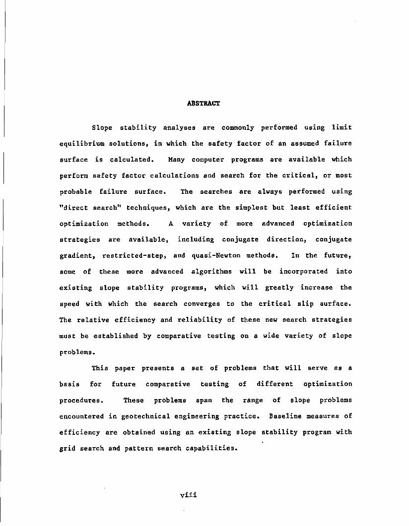
Slope stability analyses are commonly performed using limit
equilibrium solutions, in which the safety factor of an assumed failure
surface is calculated. Many computer programs are available which
perform safety factor calculations and search for the critical, or most
probable failure surface. The searches are always performed using
"direct search" techniques, which are the simplest but least efficient
optimization methods. A variety of more advanced optimization
strategies are available, including conjugate direction, conjugate
gradient, restricted-step, and quasi-Newton methods. In the future,
some of these more advanced algorithms will be incorporated into
existing slope stability programs, which will greatly increase the
speed with which the search converges to the critical slip surface.
The relative efficiency and reliability of these new search strategies
must be established by comparative testing on a wide variety of slope
problems.
This paper presents a set of problems that will serve as a
basis for future comparative testing of different optimization
procedures. These problems span the range of slope problems
encountered in geotechnical engineering practice. Baseline measures of
efficiency are obtained using an existing slope stability program with
grid search and pattern search capabilities.
viii
CHAPTER 1
INTRODUCTION
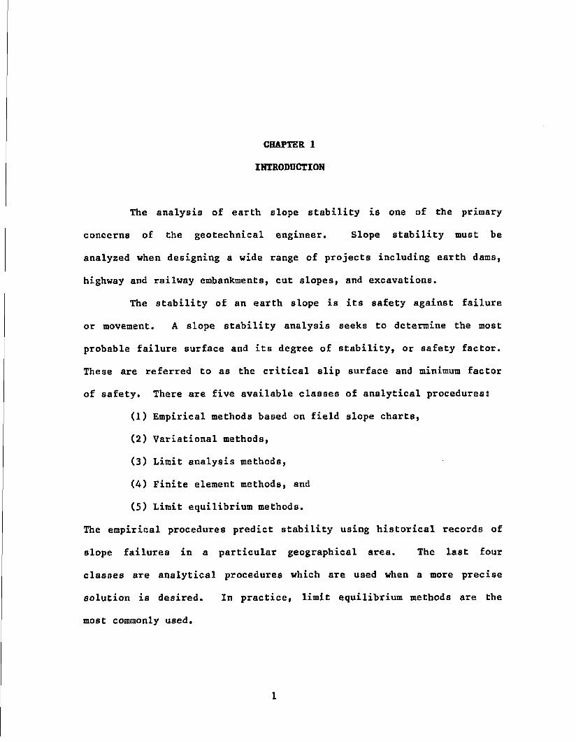
The analysis of earth slope stability is one of the primary
concerns of the geotechnical engineer. Slope stability must be
analyzed when designing a wide range of projects including earth dams,
highway and railway embankments, cut slopes, and excavations.
The stability of an earth slope is its safety against failure
or movement. A slope stability analysis seeks to determine the most
probable failure surface and its degree of stability, or safety factor.
These are referred to as the critical slip surface and minimum factor
of safety. There are five available classes of analytical procedures:
(1) Empirical methods based on field slope charts,
(2) Variational methods,
(3) Limit analysis methods,
(4) Finite element methods, and
(5) Limit equilibrium methods.
The empirical procedures predict stability using historical records of
slope failures in a particular geographical area. The last four
classes are analytical procedures which are used when a more precise
solution is desired. In practice, limit equilibrium methods are the
most commonly used.
1

2
In a limit equilibrium stability analysis, a potential failure
surface is assumed and its safety factor is calculated using one of
many available solutions. This calculation is repeated for a number of
potential failure surfaces until the minimum safety factor is found.
'Limit equilibrium solutions have been developed by Bishop, Fellinius,
Janbu, Horgenstern and Price, Lowe and Karafiath, Spencer, Taylor, the
U. S. Army Corps of Engineers, and others. Detailed examinations and
comparisons of the different methods have been made by Siegel (1975a),
Fredlund and Krahn (1977), Duncan and Wright (1980), and Fredlund,
Krahn, and Pufahl (1981).
Many computer programs have been developed to perform the
necessary safety factor calculations and to search for the critical
slip surface. The searches are always performed using "direct search"
techniques, which are the simplest but least efficient optimization
methods. In the future a variety of advanced optimization strategies
(including conjugate direction, conjugate gradient, restricted-step,
and quasi-Newton algorithms) will be incorporated into existing
programs. These algorithms will greatly increase the speed with which
the search converges to the critical slip surface. However, the
relative efficiency and reliability of these new search strategies must
be established by comparative testing on a wide variety of slope
problems. It should be noted that the theoretical accuracy of a
particular safety factor formulation (such as Bishop's or Spencer's) in
no way depends on the strategy that is implemented to guide the search
for the minimum safety factor and critical slip surface.

3
The purpose of this research is thus to develop a set of
problems to serve as a basis for the future comparative testing of
different optimization procedures. These "test functions" span the
range of slope problems encountered in geotechnical engineering
practice. Baseline measures of efficiency are obtained using an
existing slope stability program with both grid search and pattern
search capabilities.

CHAPTER 2
LITERATURE REVIEW
2.1 Existing Search Strategies. Since the advent of the
computer, geotechnical engineers have come to rely on computer codes to
analyze slope stability problems. Table 1 presents a chronological
list of many of the programs that have been developed based on limit
equilibrium solutions. Commercially available codes as well as limited
access and public domain codes written by researchers at universities,
engineering consulting firms, and government agencies are in use today.
As may be seen in Table 1, the primary difference between the
various slope stability programs lies in the method used to calculate
the factor of safety. Many of the programs use Bishop's Modified
Method, which is a highly regarded method for analyzing circular
failure surfaces. Several of the programs can be used for the analysis
of noncircular slip surfaces.
The vast majority of existing slope stability programs include
some type of routine which directs the search for the minimum safety
factor. The most commonly used search method in existing slope
stability programs is the grid search. In a grid search, a coarse
network of pointB corresponding to slip circle centers is set up over
an area large enough to include the centers of all probable failure
surfaces. It is common to initially use a relatively large and coarse
grid to get a general idea of the critical circle center location, and
4

5
TABLE 1. A COMPARISON OF AVAILABLE STABILITY PROGRAMS
Program Safety Factor Search
Name References Formulation Technique
Little & Price (1958)
Horn (1960)
ICES- Bailey ft Christian (1969)
LEASE-1 Newman (1985)
STABR Lefebvre (1971)
MALE Schiffman (1972)
Schlffnan & Jubenville (1975)
SSTAB1 Wright (1974)
SSTAB2 Chugh (1981)
SLOPE Fredlund (1974)
Fredlund & Krahn (1977)
CIVILSOFT (1976)
SLOPE-II Fredlund & Nelson (1985)
Geo-Slope (1987)
PC-SLOPE Fredlund & Nelson (1985)
Geo-Slope (1987)
STABL Siegel (1975a)
Siegel (1975b)
Siegel et al (1979)
STABL2 Boutrup (1977)
Boutrup et al (1979)
Bishop's Modified
Method
Swedish Circle
Method
Bishop's Modified
Method
Bishop's Modified
Method and Ordinary
Method of Slices
None
Pattern Search
Grid Search
Pattern Search
Morgenstern1s Method Grid Search
Spencer's Method
Spencer's Method
All State-of-the-Art
Methods
Swedish Circle Method
All State-of-the-Art
Methods
All State-of-the-Art
Methods
Bishop's Modified
Method and Janbu's
Simplified Method
Bishop's Modified
Method and Janbu's
Simplified Method
Grid Search
Grid Search
Grid Search
Grid Search
Grid Search
Randomly
Generated
Grid Search
Randomly
Generated
Grid Search

6
TABLE 1. A COMPARISON OF AVAILABLE STABILITY PROGRAMS (Continued)
Program
Name References
STABL3 Chen (1981)
STABL4 Lovell et al (1984)
PCSTABL4 Carpenter (1985)
SSDP Baker (1980)
Celestino & Duncan (1981)
Safety Factor
Formulation
Bishop's Modified
Method and Janbu's
Simplified Method
Bishop's Modified
Method and Janbu1s
Simplified Method
Bishop's Modified
Method and Janbu's
Simplified Method
Spencer's Method
Spencer's Method
Search
Technique
Randomly
Generated
Grid Search
Randomly
Generated
Grid Search
Randomly
Generated
Grid Search
Dynamic
Programming
Alternating
Variable
REAME
SWASE
Huang (1981)
Huang (1983)
Huang (1983)
Cross (1982)
Bishop's Modified
Method
Sliding Block
Bishop's Modified
Method
Grid and
Pattern Search
None
None
Nguyen (1985) Bishop's Modified
Method & Morgenstern-
Price Method
Simplex Method
of
Spendley et al
SB-SLOPE Von Gunten (1985) Bishop's Modified
Method
Grid Search
STABRG GEOSOFT (1986) Bishop's Modified
Method and Ordinary
Method of Slices
Pattern Search

7
TABLE 1. A COMPARISON OF AVAILABLE
Prograa
Naae References
SL0P8RG GEOSOPT (1986)
STABILITY PROGRAMS (Continued)
Safety Factor Search
Formulation Technique
Spencer18 Method
Handles Noncircular
Surfaces
GEOSLOPE GEOCOMP (1986) Based on STABL

8
then to construct smaller grids with finer spacings to pinpoint the
exact location of the failure surface and the precise value of the
minimum safety factor. The radii of the circles are determined from
the condition that all circles must pass tangent to a particular user-
specified elevation or through a particular user-specified point.
Figure 1 shows typical preliminary grids for slopes whose
critical slip surfaces are toe circles and base circles. Once the
computer program has evaluated the safety factors corresponding to each
point in the grid, a second smaller and finer grid is constructed
around the point with the smallest safety factor. Analyses are then
performed for circles centered at each of these new grid locations.
Sometimes, for accuracy, it may be necessary to repeat the analyses a
third time using a still smaller and finer grid. A typical three-grid
analysis is shown in Figure 2. For a slope in a layered system or in
soil whose shear strength increases with depth, the critical slip
circle will be tangent to an unknown depth. In these cases, it is
necessary to examine grids corresponding to various trial depths of
tangency.
In a grid search, the grid is either set up by the user or
generated by the computer. The STABL series of programs, developed at
Purdue University, usea. random, computer-generated grids. In this
technique, described by Boutrup et al. (1979), trial piecewise-linear
failure surfaces are generated from a series of starting points with
equal horizontal spacing along the ground surface at the base of the
slope. The failure surface is defined by a series of line segments

9
grid spacing
slip circle centers <
5a» potential failure surfaces
(a) Toe Circles
(b) Base Circles
Figure 1. Typical Grids for Grid Searches

10
Lowest value in grid
Second grid
(a) Initial (coarse) Grid
Lowest value in grid
Final grid
(b) Second (finer) Grid
True minimum
(c) Final Grid
Figure 2. A Typical Three-Grid Analysis

11
beginning at these starting points. The orientations of these line
segments are defined as functions of direction limits and a random
number function. The user specifies the number of trial surfaces
desired, and the computer plots the ten surfaces having the lowest
safety factors.
The grid search method is useful in determining safety factor
values for many specified circle centers. With this information, it
becomes possible to plot contours of equal safety factor values. This
information may be helpful when analyzing problems which have more than
one local minimum safety factor. Such a situation is depicted in
Figure 3. The major disadvantage of the grid search procedure is its
inherent slowness. The trial evaluation points are always preselected
by the analyst, and thus the efficiency of the technique depends solely
on the expertise and insight of the user. It may take several trials
to identify the true tangent depth of the critical circle. Once this
has been established, further grid refinements may be required to
ensure that the true minimum safety factor has been determined.
A second common search method is the pattern search, which is
included in the STABR (Lefebvre, 1971) and REAME (Huang, 1981 and 1983)
programs. It is similar to the grid search in that a fixed circle
center spacing or "step length" is predetermined by the user. In the
STABR program, the coordinates of the center of the first circle to be
analyzed are specified on input. The safety factor is calculated for
this center and for centers spaced symmetrically around it, as shown in
Figure 4a. The centers are generated in the order shown by rotating

12
2.0
1.8 F= 1.75
Figure 3. Example of a Slope With Two Local Minimum Safety Factors (after Duncan and Buchignani, 1975)

4
1
2
(a) First clockwise rotation around the given center, A. The rotation starts at point 1, with radius of rotation twice the final step length.
x -*
(b) The 45-degree clockwise rotation around the center, B. The rotation starts at point 1, with radius of rotation 1.414 times the final step length.
Figure 4. The Pattern Search Method Used in STABR (after Lefebvre, 1971)

14
around the specified center with a radius of rotation equal to twice
the specified final step length. If a safety factor less than that at
the center of rotation is found for any point, that point becomes the
new center of rotation. If a full rotation is completed and no safety
factor smaller than that at the center of rotation is found, the length
of the search circle radius is reduced to the final step length and a
second 4-point rotation is performed. If a smaller safety factor is
still not found, another rotation around the same center is initiated,
starting at a 45-degree angle with a search circle radius length of
1.414 times the final step length, as shown in Figure 4b. After a
tentative minimum safety factor is found, it may be necessary to repeat
the analysis using a smaller step length in order to further pinpoint
the center of the true critical circle. It is often necessary to
repeat this process for several different tangent elevations, since the
depth to which the critical circle is tangent is unknown for many
problems.
Figure 5 shows a typical path taken by the STABR pattern search
routine. The search path is superimposed on a safety factor contour
plot. Each point represents—a- safety factor evaluation for a
particular circle center. In this example, 25 trials were
automatically performed to reach the actual minimum, then seven more
evaluations to verify that the minimum had been found. As Figure 5
shows, several centers were evaluated twice during the search (for
example, Points 11 and 14, Points 17 and 20, etc.), which causes
unnecessary delay and computer expense.

15
safety factor contours
minimum safety factor = point 25
Figure 5. A Typical STABR Search Path
16
The pattern search method represents a major improvement over
the grid search, since the computer does much more of the work in
identifying the critical slip surface. However, the method has several
drawbacks. If the tangent depth for the critical slip surface is
unknown, several trials are needed to locate the actual critical
tangent elevation, just as in the grid search method. As shown in
Figure 5 and discussed above, the path followed by a pattern search can
often be quite inefficient. If the starting point of the search is far
from the actual critical center, many evaluations are needed to find
the minimum safety factor, since the step length does not vary. In
addition, the minimum may not always be identified, as the total number
of evaluations is generally limited by the particular program being
used. Even if a minimum is identified, it may be necessary to repeat
the analysis using a still smaller step length in order to further
pinpoint the center coordinates.
A limited variety of other direct search procedures have also
been used in conjunction with slope stability analyses. Celestino and
Duncan (1981) used the alternating variable method to search for the
critical piecewise linear slip surface. In the alternating variable
method, the search for a minimum safety factor is accomplished by
searching in directions parallel to each coordinate axis and then
changing directions each time a minimum is located. A diagram of a
typical alternating variable search is shown in Figure 6.
Nguyen (1985) recently applied an early version of the simplex
method to slope stability analysis. In this method, a regular simplex
(n + 1 mutually equidistant points, where n defines the number of

17
Figure 6. Alternating Variable Search Method (after Swann, 1972)

18
independent variables) is set up and the safety factor is evaluated at
each vertex. An iteration consists of replacing the vertex associated
with the highest safety factor value with its mirror image about the
centroid of the remaining vertices. More recently, Awad (1986) adapted
the more efficient simplex method of Nelder and Mead (1965) to slope
stability analysis. In the method of Nelder and Mead (1965), the
regularity of the simplex design is abandoned, and the simplex
automatically rescales itself by expanding or contracting according to
the local geometry of the function. The family of simplex methods is
generally regarded as the most efficient of direct search techniques
(Swann, 1972).
This literature review examined all slope stability codes
mentioned in the literature as well as many commercially available
codes. While several direct search optimization methods have
successfully been used, no advanced optimization techniques have ever
been incorporated into slope stability analysis programs. The merits,
limitations, and general requirements of these more advanced classes of
optimization techniques may now be briefly described.
2.2 Available Optimization Techniques. An optimization
routine is designed to search for the minimum value of the function
being examined. Many search algorithms have been developed, and they
can be classified based on the level of information that is required to
direct the search. They can be categorized as follows (DeNatale,
1983):

19
(1) Second derivative (or Newton) methods,
(2) Quasi-Newton methods,
(3) Discrete (or finite-difference) Newton methods,
(4) Restricted step (or trust-region) methods,
(5) Conjugate gradient and conjugate direction methods,
(6) Direct search (or ad hoc) methods, and
(7) Sum of squares methods.
The classes of algorithms have been arranged roughly in order of
decreasing efficiency, with second derivative methods being the most
efficient, and with direct search routines being the slowest and most
basic. The exception is the sum of squares methods, which are
advantageous in certain limited applications. A thorough discussion of
the merits and shortcomings of the various general classes of
optimization techniques is presented by DeNatale (1983), and a summary
of this discussion is given in Table 2.
The safety factor expression in a generalized limit equilibrium
procedure (such as in a Bishop's or Spencer's analysis) is
nondifferentiable. Therefore, gradient and curvature expressions are
not explicitly available. However, finite-difference procedures can be
used to calculate derivatives, and all classes of optimization
algorithms could potentially be used in conjunction with slope
stability analyses. In fact, it is very likely that the more advanced
techniques, such as the quasi-Newton methods, may be the most efficient
overall, despite the additional trials associated with derivative
calculations by finite-differences (DeNatale, 1983).

20
TABLE 2 , A COMPARISON OF THE VARIOUS CLASSES OF OPTIMIZATION TECHNIQUES
Class Requirements Advantages Disadvantages
Second
Derivative
Methods
•function
•gradient
•curvature
•superlinear
convergence
•self-corrective
•possible to
distinguish between
local minima and
saddle points
••ay not converge
from poor initial
guess
•requires second
derivatives
•requires solution
of n-linear equations
at each iteration
Discrete
Newton
Methods
•function
•gradient
•sane as for
Second Derivative
Methods
•inefficient for
large-dimension
problems
•optimal differencing
Intervals must be
determined
Quasi-
Newton
Methods
•function
•gradient
•requires first
derivatives only
•no equation solving
is required
•round-off errors can
have large effect on
performance
Restricted
Step
Methods
•function •excellent
convergence
•requires many arith
metic operations
Conjugate
Direction
and
Conjugate
Gradient
Methods
•function •requires little
core memory
•few arithmetic
operations per
iteration
•excellent for
large problems
•less efficient and
robust than Newton-
type methods
Direct
Search
Methods
•function •extremely general
and simple to code
•immune from
rounding errors and
ill-conditioning
•requires little
core memory
•rather slow
convergence
•function
evaluations increase
exponentially with
the dimension of the
problem
•a large number of user
specified constants
is required

CHAPTER 3
MATERIALS AND METHODS
3.1 Modelling Slope Stability Problems for Optimization.
Before optimization techniques can be used with slope stability
programs it is necessary to characterize slope problems as optimization
problems. This may be done by analyzing the general classes of
stability problems to determine the number of independent variables (or
dimensions) to be searched for each type of problem. General
characterizations are shown in Figure 7.
Figures 7a and 7b show planar slip surfaces. The general case
involves two independent variables, these being the angle of
orientation of the slip surface and the height above the toe at which
this surface intersects the slope face. For the special case of a
plane passing through a fixed point, such as the toe of the slope, the
critical angle of inclination is the only quantity that would need to
be identified.
Figures 7c, 7d, and 7e show circular failure surfaces. In
general, a problem involving circular slip surfaces is a three-
dimensional problem. The three degrees of freedom are the x- and y-
coordinates of the circle center and its radius. For certain cases
circular slip surfaces can be analyzed as two-dimensional problems. In
a purely cohesive (<{> = 0) soil with a slope angle greater than
53 degrees, the critical circle passes through the toe of the slope
21

22
one degree of freedom: inclination of slip surface
(a) Plane Through Toe
two degrees of freedom: slip surface inclination, height above toe of intersection with slope face
(b) Any Planar Slip Surface
two degrees of freedom: x- and y- coordinates of circle center
(c) Circle Through Toe
Figure 7. Slope Stability Models

23
two degrees of freedom: x- and y- coordinates of circle center
(d) Circle Tangent to Firm Stratum
three degrees of freedom: x- and y- coordinates of circle center, radius of
circle
(e) Any Circular Slip Surface
X.
2s degrees of freedom, where s = number of line segments defining slip surface
(f) Piecewise Linear Slip Surface
Figure 7. (continued)

24
(Terzaghi, 1943), as shown in Figure 7c. In a purely cohesive (<f> = 0)
soil with a slope angle less than 53 degrees, the critical circle
passes tangent to the top of the underlying firm stratum (Terzaghi,
1943), as shown in Figure 7d. In both cases the radius of the circle
is fixed once the x-and y-coordinates of the center are selected.
Another type of slope problem is one which has a piecewise-
linear slip surface. The general case is shown in Figure 7f. This
type of problem involves 2s degrees of freedom, where s is the number
of line segments used, and where the orientation and length of each
segment become the independent variables. Composite circular-linear
surfaces are also possibilities.
3.2 Example Problems. In optimization research, analytic
"test functions" are normally used to evaluate the relative merits and
limitations of competing search strategies. A large number of these
functions have been developed, and many are described by Cornwell
et al. (1980). A similarly wide range of problems is developed herein,
with the following purposes in mind: (1) to find a set of problems
which represent typical slope stability problems encountered in
geotechnical engineering practice, and (2) to pinpoint those problems
in which direct search methods present severe limitations or give
inaccurate results. The following types of problems are therefore
considered:
(1) Steep slopes in homogeneous soils,
(2) Mild slopes in homogeneous soils,
(3) Slopes in soils whose shear strength increases with depth,

25
(4) Problems with a stepped slope face,
(5) Slopes in stratified soil deposits, and
(6) Published case histories that have been examined by others.
One aspect of special interest in choosing these example problems was
to identify those conditions that result in multimodality, or the
existence of more than one local minimum safety factor.
3.3 The STABR Slope Stability Program. The STABR slope
stability program developed by Lefebvre (1971) is used in the present
study. It analyzes circular failure surfaces using both Bishop's
Modified Method and the Ordinary Method of Slices. The program can be
used for both total and effective stress analyses. (A total stress
analysis uses the undrained strength parameters c and $ to
establish the short-term stability of the slope. An effective stress
analysis uses the drained strength parameters c* and to estimate
the long-term stability of the slope.) It is capable of handling
irregular slope profiles, tension cracks, soil layers with different
properties and nonuniform thicknesses, complicated pore pressure
patterns, variation of undrained strength with depth, and seismic
forces.
As mentioned previously, a pattern search routine is included
in the STABR program. To employ the search routine the user must
specify either a horizontal line to which all slip circles are tangent
or a specific point through which all circles pass. Additional
information needed by the program includes the coordinates of the

26
center of the initial circle and the final step length desired. To
minimize the number of evaluations, the User'B Manual recommends that a
fairly large step length be used initially, so that the approximate
center of the critical circle can be found with relatively few circle
analyses (Lefebvre, 1971). The program can then be rerun using a finer
step length to pinpoint the critical circle center with more accuracy.
A modified version of the program has also been developed by DeNatale.
In this version the pattern search strategy is replaced with the basic
grid search procedure.
3.4 Criteria for Evaluating Relative Merits of Different
Search Strategies. The test problems may be used to compare two
different search strategies by analyzing the same problem using each of
the two different search techniques and then comparing the results for
accuracy and efficiency. Items which should be included in a
comparison of two methods are (1) the effect of starting point (a
reflection or indication of user expertise), and (2) the effect of grid
spacing (in the grid search methods) or step size (in the pattern
search methods). The effects of these factors should be examined
through a parametric study. Since the number of arithmetic operations
used by any optimization scheme to select a trial evaluation point (or
circle center) is always small relative to the number of operations
needed to compute the safety factor, the number of trial evaluation
points required to locate the minimum safety factor is used as the
basis for evaluating efficiency. It is desirable to obtain a minimum
value using the least number of evaluation points in order to reduce
the total computer time.

CHAPTER 4
PRESENTATION OF RESULTS
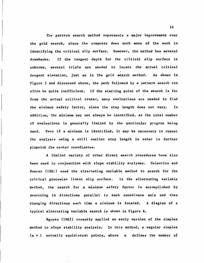
4.X Steep Slope in Homogeneous Soil. The first problem
studied is a slope in homogeneous, cohesive soil with a slope angle of
60 degrees, as shown in Figure 8. It is known that the critical circle
will pass through the toe of the slopet since a <t* = 0 shear strength
characterization is being used and the slope is steep (Terzaghi, 1943).
These features cause the problem to reduce to two-dimensional search
for the critical safety factor.
The location of the critical circle center was first identified
by running the STABR program for a one-foot step length. A grid of
circle centers at five-foot intervals was then set up around the
critical center in order to identify the safety factor contours. The
contour plots in Figure 9 show a regular contour pattern with a single
minimum safety factor.
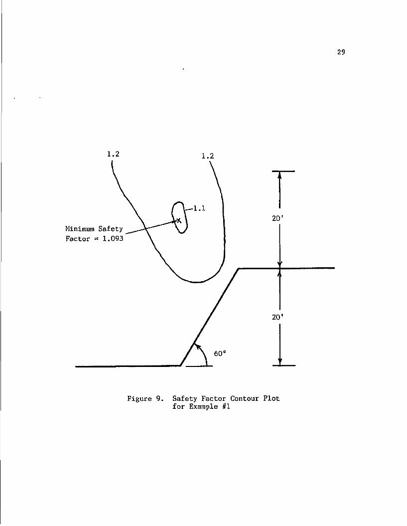
The other factors studied for this problem are the effects of
starting point and grid size (or step length) on the total number of
function evaluations required in both grid and pattern searches. To
define errors in the initial grid size and spacing for grid searches,
four levels of expertise are defined using the following four grid
logics:
27

28
(100,100)
60 (111.55,120)
120 pcf
500 psf
40'
Figure 8. Example #1 - Steep Slope
29
! - 2 1 . 2
20*
Minimum Safety
Factor - 1.093
60
Figure 9. Safety Factor Contour Plot for Example #1

30
Initial Grid Logic
Side Length of Grid Perimeter
Initial
Grid Size Intermediate
Grid Size Final
Grid Size
Expert 30% 6% Rcc 1 ft
Good 60S: Rcc 9% Rcc 1 ft
Fair 130% Rcc 13% Rcc 6% Rgg 1 ft
Poor 200% Rcc 20% Rcc 6% Rcc 1 ft
The grid perimeters and grid sizes are shown in Figure 10. As may be
seen, the initial grid is always centered about the true critical
center. All initial grids extended vertically downwards to the level
of the top of the slope. Rcc is defined as the radius of the critical
circle.
The choices of expert, good, fair, and poor grid logics are
subjective. They are intended to model the various abilities and
degrees of experience of slope stability analysts. Someone with little
or no previous experience in the area of slope stability would be less
likely to choose a small initial grid close to the actual critical
center than a person with a great deal of experience in analyzing
slopes. The better grid logics (expert and good) do not require an
intermediate grid because they are fairly close to the critical center
initially.
To define errors in starting points for pattern searches, four
levels of expertise are defined, based on the distance of the starting
point from the actual critical center:
31
Initial Grid Perimeter Side Length1-1''
Lowest value in grid-
1—*—f
J I
I Initial Grid Size
Intermediate Grid Perimeter Side Length ( = 2 times initial grid size)
' ̂ Intermediate Grid Size
•Lowest value in grid
Final Grid Perimeter Side Length ( = 2 times intermediate grid size)
Final Grid Size (1 ft.)
True minimum
Figure 10. Sizes and Sequences Used in the Grid Searches

32
Type of Estimate
Expert
Good
Initial Distance Error
Upper corners of expert initial grid
Poor
Fair
Upper corners of good initial grid
Upper corners of fair initial grid
Upper corners of poor initial grid
The initial grids and starting points for this problem are shown in
Figure 11. In order to obtain representative measures of efficiency,
two different starting points were examined for each of the four levels
of expertise. The following two step length refinement logics are used
with each level of expertise:
Step Length Refinement Logic A
Trial 1 - Start the search at the predetermined starting point.
Use a 5 ft final step length.
Trial 2 - Start the search at the critical center determined
in first trial. Use a 2 ft final step length.
Trial 3 - Start the search at the critical center determined
in second trial. Use a 0.5 ft final step length.
Step Length Refinement Logic B
Trial 1 - Start the search at the predetermined starting point.
Use a 5 ft final step length.
Trial 2 - Start the search at the critical center determined
in first trial. Use a 0.5 ft final step length.
These two step length refinement logics are intended to define two
strategies of different effectiveness. The relative superiority of

33
poor initial grid 39,62)
(129,72) fair initial grid-^ (91,72)
(119,82) ,82)
(114,87) (96,87)
(110,91)
(100,100)
(111.55,120)
Figure 11. Initial Grids and Starting Points for Example #1

34
each refinement logic may depend on the closeness of the initial
starting point.
The total number of safety factor evaluations required in any
given pattern search analysis is obtained by adding together the number
of function evaluations performed in each trial of a given step length
logic. The total number of function evaluations required in any
particular grid search analysis is obtained by adding together the
number of function evaluations performed for each grid size (i.e.,
initial, intermediate, final) for each type of estimate.
Table 3 gives the results of the various pattern search
analyses. The average number of function evaluations for each level
of expertise and step length logic is summarized in Table 4A. Table 4A
shows that the number of function evaluations required to identify the
critical center decreases as the starting error decreases. An
examination of Table 4A also shows that the expert and good starting
points require about the same number of function evaluations. However,
once the starting error increases past the good level of expertise,
efficiency decreases rapidly, especially for Step Length Refinement
Logic B.
The relative efficiency of the two step length refinement
logics depends on the distance of the starting point from the actual
critical center. This is clearly shown in Table 4A. When the starting
guess is fairly close (expert and good levels of expertise), Step
Length Refinement Logic B is the more efficient logic. When the
starting guess is far from the critical center (fair and poor levels of

35
TABLE 3
PATTESM SEARCH RESULTS FOR EXAMPLE #1
Trial Starting
Point (ft)
Step Length Logic
Total No.
of Function Evaluations
Minimum F.S.
1 (139,62) A 59 1.093
2 (139,62) B 74 1.093
3 (81,62) A 63 1.093
4 (81,62) B 77 1.093
5 (129,72) A 47 1.093
6 (129,72) B 54 1.093
7 (91,72) A 50 1.093
8 (91,72) B 54 1.093
9 (119,82) A 47 1.093
10 (119,82) B 34 1.093
11 (101,82) A 39 1.093
12 (101,82) B 36 1.093
13 (114,87) A 44 1.093
14 (114,87) B 34 1.093
15 (96,87) A 41 1.093
16 (96,87) B 32 1.093
(x,y) Radius of Minimum (ft)
(111,91),29
(111,91),29
(111,91),29
(111,91),29
(111,91),29
(111,91),29
(111,91),29
(111,91),29
(111,91),29
(111,91),29
(111,91),29
(111,91),29
(111,91),29
(111,91),29
(111,91),29
(111,91),29

TABLE 4A
EFFECT OF STEP LEHGTH LOGIC ON EFFICIENCY FOR EXAMPLE fl
Starting Step Length Average Number of Guess Logic Function Evaluations
Poor A 61 B 76
Fair A 49 B 54
Good A 43
B 35
Expert A 43
B 33
TABLE 4B
EFFECT OF EXPERTISE ON EFFICIENCY FOR EXAMPLE #1
Starting Guess
Step Length Logic
Number of Function Evaluations
Poor B only 76
Fair A-B average 52
Good A-B average 39
Expert B only 33

37
*
expertise), Step Length Refinement Logic A is the more efficient logic.
Logic B requires more function evaluations for the poorer starting
points since the intermediate step length refinement is omitted. The
expert, good, fair, and poor analyses could be further quantified by
assuming that .a person who uses an expert starting point would also use
the most efficient step length refinement logic (Logic B), a person who
uses a poor starting point would also use the least efficient step
length refinement logic (Logic B), and that persons who use
intermediate starting points would use intermediate logics (the average
of Logics A and B). With such assumptions, it becomes possible to
develop Table 4B.
Table 5 presents the results of the grid search analyses. Once
again the size of the initial and subsequent grids has a large effect
on the total number of function evaluations. About twice as many
evaluations are required as the level of expertise decreases from
expert to poor. A comparison of Tables 4B and 5 reveal that many more
function evaluations are required by the grid search than by the
pattern search for any given level of expertise.
4.2 Mild Slope in Homogeneous Soil. The second problem
studied is a slope in homogeneous cohesive soil with a slope angle of
30 degrees, underlain by a firm stratum, as shown in Figure 12. It is
known that the critical circle is tangent to the top of the firm layer
(Terzaghi, 1943). Therefore, this problem again reduces to a two-
dimensional search for the minimum safety factor.

38
TABLE 5
GRID SEARCH RESOLTS FOR EXAMPLE #1
Grid Total Number of Mininum (x,y) Radius of Logic Function Evaluations F.S. Critical Circle (ft)
Expert 75 1.093 (111,90),30
Good 98 1.093 (111,90),30
Fair 130 1.093 (111,90),30
Poor 144 1.093 (111,90),30

39
(100,100)
30'
(152,130)
"Jf = 120 pcf s!= o
c = 800 psf 30'
Figure 12. Example #2 - Mild Slope

40
Grid and pattern searches are once again used to identify the
critical circle, and the effect of varying the initial grid size and
starting point is again studied. The previously defined initial gridB,
starting errors, and refinement logics are used. Specific initial
grids and starting points are shown in Figure 13.
The results of the various pattern searches are given in
Table 6, and the average number of function evaluations for each level
of expertise and step length refinement logic is summarized in
Table 7A. The results presented in Tables 7A and 7B reveal that many
more function evaluations are required to find the minimum safety
factor as the starting point is moved farther from the actual critical
center. The magnitude of the starting error has a more pronounced
effect on efficiency in this problem than in the toe circle problem,
Example #1. This is because the larger critical circle radius in this
problem caused the starting points to be farther from the actual
critical center than in Example #1.
Table 8 gives the results of the grid searches. As with
Example #1, more function evaluations are once again needed for a grid
search than for a pattern search. In this problem, the good grid logic
required more safety factor evaluations than any of the other levels of
expertise. This is because an intermediate grid refinement is not
used, and the one-foot final grid required a large number of
evaluations due to the magnitude of the critical circle radius, Rcc.
4.3 Slope in Stratified Soil. Example #3 consists of a slope
in cohesive soil with an intermediate sand layer. The soil profile is

(210.5,-9) poor initial grid
(41.5,-9)
fair initial gridN
(181,20.5) 1 (71,20.5)
goor initial grid, (151,50.5)
grill/
yaoi.50.5)
(138.5,63)(113.5,63)
7^ \ (126,75.5) ̂ -expert initial grid (100,100)
(152,13C
Figure 13. Initial Grids and Starting Points for Example #2

42
TABLE 6
PATTERN SEARCH RESULTS FOR EXAMPLE #2
Trial
Starting Point (ft)
Step Length Logic
Total No. of Function Evaluations
Minimum
F.S.
(x,y) Radius of Critical Circle
(ft)
1 (210.5,-9) A 96 1.289 (126,75.5),84.5
2 (210.5,-9) B 178 1.289 (126,75.5),84.5
3 (41.5,-9) A 80 1.289 (126,75.5),84.5
4 (41.5,-9) B 140 1.289 (126,75.5),84.5
5 (181,20.5) A 73 1.289 (126,75.5),84.5
6 (181,20.5) B 132 1.289 (126,75.5),84.5
7 (71,20.5) A 63 1.289 (126,75.5),84.5
8 (71,20.5) B 108 1.289 (126,75.5),84.5
9 (151,50.5) A 51 1.289 (126,75.5),84.5
10 (151,50.5 B 75 1.289 (126,75.5),84.5
11 (101,50.5) A 47 1.289 (126,75.5),84.5
12 (101,50.5) B 65 1.289 (126,75.5),84.5
13 (138.5,63) A 45 1.289 (126,75.5),84.5
14 (138.5,63) B 47 1.289 (126,75.5),84.5
15 (113.5,63) A 41 1.289 (126,75.5),84.5
16 (113.5,63) B 39 1.289 (126,75.5),84.5

TABLE 7A
EFFECT OF STEP LENGTH LOGIC ON EFFICIENCY FOR EXAMPLE #2
Starting Step Length Average Number of Guess Logic Function Evaluations
Poor A 61
B 76
Fair A 49 B 54
Good A 43
B 35
Expert A 43
B 33
TABLE 7B
EFFECT OF EXPERTISE ON EFFICIENCY FOR EXAMPLE #2
Starting Step Length Number of Guess Logic Function Evaluations
Poor B only 159
Fair A-B average 94
Good A-B average 60
Expert B only 43

44
TABLE 8
GRID SEARCH RESULTS FOR EXAMPLE #2
Grid Logic
Total Number of Function Evaluations
Minimum F.S.
(xfy) Radius of Critical Circle (ft)
Expert 157 1.289 (125.5,74),86
Good 338 1.289 (126,75.5),84.5
Fair 234 1.289 (126,75.55,84.5
Poor 240 1.289 (125.5,74),86

45
shown in Figure 14. In this type of problem, the depth to which the
critical circle is tangent is unknown. However, slope stability theory
predicts that the critical circle will pass tangent to a boundary
between two layers rather than at some point within a layer (Taylor,
1948). The STABR program was run specifying three different depths of
tangency. The results of the three searches are shown in Figure 15.
It can be seen that the minimum safety factor occurred for the slip
circle tangent to the top of the sand layer.
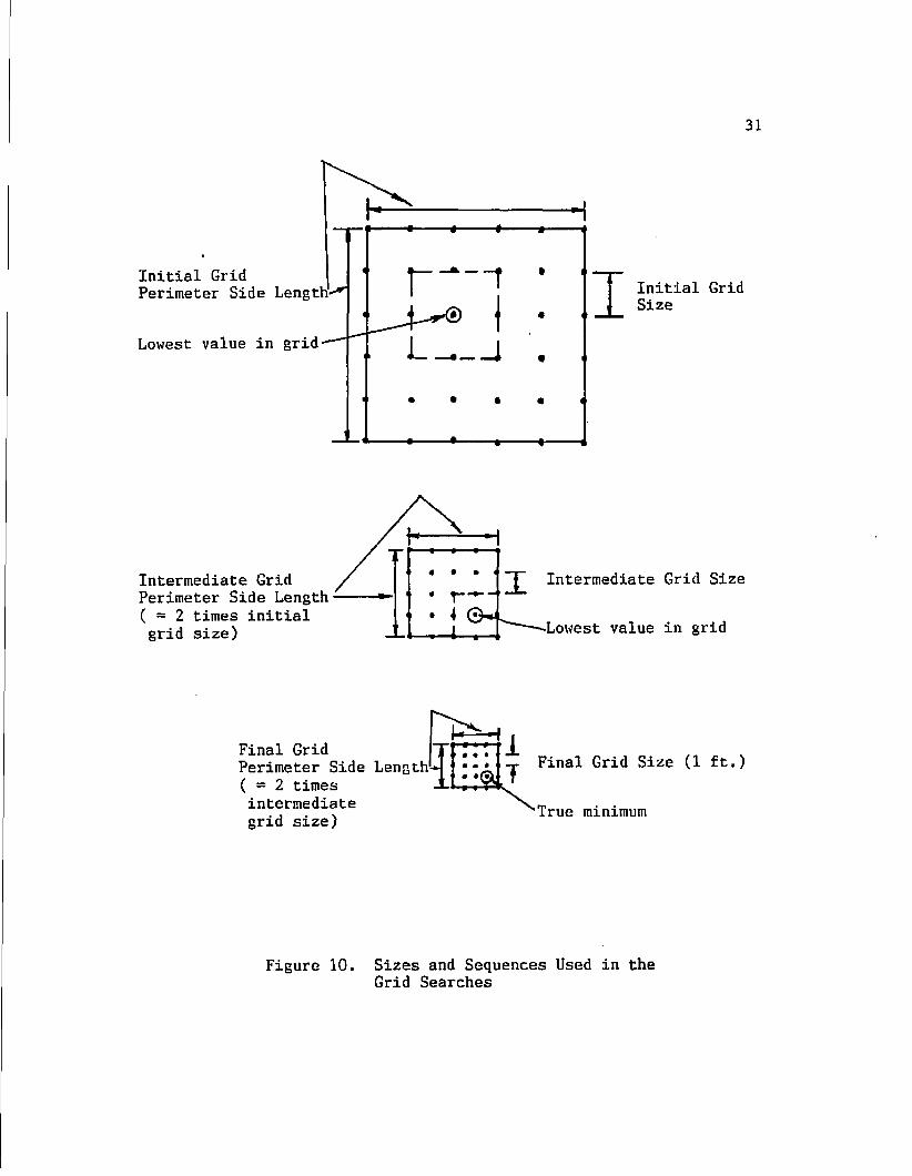
The variation in safety factor was studied by evaluating the
safety factors for a given circle center while varying the depth of
tangency. The variation in safety factor with depth is shown in
Figure 16 for three circle centers along the critical vertical section.
As may be seen, the safety factor decreases as the depth of the circle
is lowered until the minimum value is reached at the top of the sand
layer. The safety factor increases for circles passing through the
sand layer, then decreases again as the tangent depth passes through
the lower cohesive layer. This shows a multimodal type of behavior or
the existence of more than one local minimum safety factor.
The effects of initial grid size, starting point, and refinement
logic are examined by the techniques previously described in
Section 4.1. Figure 17 shows the specific initial grids and starting
points, and Table 9 presents the results of the various pattern
searches. The average number of function evaluations for each level of
starting guess and refinement logic are summarized in Table 10A. As
may be seen from Tables 10A and 10B, more than twice the number of

(100,100)
20'
(135,120)
IS = 120 pcf / - 0 10* c = 500 psf
= 120 pcf, ff = 30°, c = 0 5'
y = 120 pcf / = 0 15' c = 500 psf
Figure 14. Example #3 - Stratified Soil Deposit

min
rain 2.224
= 1.417 raxn
Figure 15. Critical Circles for Three Different Tangent Elevations
*-sJ
48
Safety
Factor
4.0
3.0
2 .0
Sand layer
1 . 0 110
3.0
2 . 0 '
1 . 0
3.0
2.0
1 . 0
Circle Center (115,85)
Circle Center (115,80)
110 120 130 140 150
Circle Center (115,75)
110 130 150
Depth (ft.)
Figure 16. Variation in Safety Factor with Depth for Example #3

(161,43) poor initial grid
1 (74,73)
fair initial grid-* (145.5,58.5) \ (89.5,58.5)
good initial grid* (130.5,73.5) ^104.5,73.5)
124,80)(111,80)
—a—».
(117.5,86.5) —expert initial grid
(100,100)
(134.6,120)
Figure 17. Initial Grids and Starting Points for Example #3

50
TABLE 9
PATTERN SEARCH RESULTS FOR EXAMPLE #3
Trial Starting
Point (ft)
Step
Length Logic
Total No. of Function Evaluations
Minimum
F.S.
(xfy) Radius of Minimum (ft)
1 (161,43) A 69 1.271 (117.5,86.5),43.5
2 (161,43) B 98 1.271 (117.5,86.5),43.5
3 (74,73) A 49 1.271 (117.5,86.5),43.5
4 (74,73) B 50 1.271 (117.5,86.5),43.5
5 (145.5,58.5) A 54 1.271 (117.5,86.5),43.5
6 (145.5,58.5) B 70 1.271 (117.5,86.5),43.5
7 (89.5,58.5) A 51 1.271 (117.5,86.5),43.5
8 (89.5,58.5) B 58 1.271 (117.5,86.5),43.5
9 (130.5,73.5) A 44 1.271 (117.5,86.5),43.5
10 (130.5,73.5) B 49 1.271 (117.5,86.5),43.5
11 (104.5,73.5) A 42 1.271 (117.5,86.5),43.5
12 (104.5,73.5) B 42 1.271 (117.5,86.5),43.5
13 (124,80) A 46 1.271 (117.5,86.5),43.5
14 (124,80) B 35 1.271 (117.5,86.5),43.5
15 (111,80) A 44 1.271 (117.5,86.5),43.5
16 (111,80) B 30 1.271 (117.5,86.5),43.5

TABLE 10A
EFFECT OF STEP LENGTH LOGIC ON EFFICIENCY FOR EXAMPLE #3
. Starting Step Length Average Number of Guess Logic Function Evaluations
Poor A 59 B 74
Fair A 53 B 64
Good A 43 B 46
Expert A 45 B 33
TABLE IOB
EFFECT OF EXPERTISE ON EFFICIENCY FOR EXAMPLE #3
Starting Guess
Step Length Logic
Number of Function Evaluations
Poor B only 74
Fair A-B average 59
Good A-B average 44
Expert B only 33

52
function evaluations are required as the level of expertise decreases
from expert to poor. Grid search analyses were not performed.
It should be noted that the particular study described above
assumed that the actual critical tangent elevation was known. Finding
the critical depth is actually the first step in solving for the
minimum safety factor. One could get some idea of the total number of
function evaluations needed in any analysis by multiplying the values
shown in Tables 10A and 10B by the number of tangent elevations
searched (in this case, three).
4.4 Birch Dam. The fourth example studied was Birch Dam, a
case history which has also been examined by Gelestino and Duncan
(1981) and Nguyen (1985). The soil configuration is shown in
Figure 18. Celestino and Duncan found the critical slip surface to be
a base circle tangent to the top of the firm stratum. This was
verified by running STABR searches using a variety of different trial
tangent elevations.
Figure 19 shows the initial grids and starting points for the
various levels of expertise. The pattern searches are presented in
Table 11 and the average number of function evaluations are summarized
in Table 12A. Table 12B presents the effect of expertise on the
efficiency of the pattern searches. In studying these results, it can
be concluded that both starting point and step length have a pronounced
effect on the total number of function evaluations required to find the
minimum safety factor. In all but the expert starting guess in
Table 12A, step length refinement logic B required up to twice as many

53
(100,100)
c = 1023 psf X = 3 1 ° ,
Y = 127 pcf/
c = 1629 psf / = 18° Y = 127 pcf
(245,157) c = 1023 pcf 37'
Y = 127 pcf
Figure 18. Example #4 - Birch Dam

(297,-49) poor initial grid'
(54,-49)
(254.5,-6.5) fair initial grid
) (96.5,-6.5)
good initial grid (212,36) ^ (139,36)
(193.5.54.5)(157.5.! 4.5)
(175.5,72.5) •expert initial grid (100,100)
(245,157)
Figure 19. Initial Grids and Starting Points for Example #4
in

55
TABLE 11
PATTERN SEARCH RESULTS FOR EXAMPLE #4
Trial
Starting Point (ft)
Step
Length Logic
Total No. of Function Evaluations
Minimum
F.S.
(x,y) Radius of
Critical Circle (ft)
1 (297,-49) A 127 1.096 (175.0 73.5) 120.5
2 (297,-49) B 259 1.096 (175.0 73.5) 120.5
3 (54,-49) A 118 1.096 (174.0 75.5) 118.5
4 (54,-49) B 237 1.097 (175.5 72.5) 121.5
5 (254.5,-6.5) A 93 1.096 (174.5 74.5) 119.5
6 (254.5,-6.5) B 179 1.097 (175.5 72.5) 121.5
7 (96.5,-6.5) A 94 1.097 (175.5 72.5) 121.5
8 (96.5,-6.5) B 172 1.097 (175.5 72.5) 121.5
9 (212,36) A 69 1.096 (175.0 73.5) 120.5
10 (212,36) B 95 1.097 (175.5 72.5) 121.5
11 (139,36) A 66 1.096 (174.0 75.5) 118.5
12 (139,36) B 100 1.096 (175.0 73.5) 120.5
13 (193.5,54.5) A 51 1.097 (175.5 72.5) 121.5
14 (193.5,54.5) B 56 1.097 (175.5 72.5) 121.5
15 (157.5,54.5) A 62 1.096 (174.5 74.5) 119.5
16 (157.5,54.5) B 60 1.097 (175.5 72.5) 121.5

TABLE 12A
EFFECT OF STEP LENGTH LOGIC ON EFFIClEHCT FOR EXAMPLE #4
Starting Guess
Poor
Fair
Good
Expert
Step Length Logic
A
B
A
B
A
B
A
B
Average Number of
Function Evaluations
123 248
94 176
68 98
57 58
TABLE 12B
EFFECT OF EXPERTISE OH EFFICIENCY FOR EXAMPLE #4
Starting Guess
Poor
Fair
Good
Expert
Step Length Logic
B only
A-B average
A-B average
A only
Number of Function Evaluations
248
135
83
57

57
function evaluations as step length refinement logic A. This suggests
that a larger initial step length would increase the efficiency of the
search even though two further grid refinements are needed instead of
one. This is due to the fairly large scale of this problem and the
resulting relatively large value for the critical circle radius Rcc*
A comparison of the various levels of expertise of starting guess shows
that a poor initial guess requires from two to four times more
function evaluations than an expert guess, depending on which step
length logic is used.
It may be noted in Table 11 that the coordinates and radius of
the critical circle and their corresponding safety factors vary
slightly. This is because the minimum safety factor occurs for a range
of points rather than for a single point. The fixed step length in the
pattern search causes the search to end at slightly different points.
The difference in safety factors is due to the number of significant
digits used in the STABR analysis.
4.5 Slope in Soil with Continuous Variation of Strength. The
fifth problem studied was a slope in soil whose strength increases
linearly with depth, shown in Figure 20. In this type of problem, the
depth to which the critical circle is tangent is unknown. To locate
the critical depth, searches were performed at several widely spaced
tangents. The resulting critical circles are shown in Figure 21. This
showed the lowest safety factor occurring for a circle tangent to a
depth 20 feet below the top of the slope. Further searches were then

c = 200 psf
(100,100)
20'
(134.64,120)
V = 120 pcf
100'
_ L _
^ c = 800 psf
Figure 20, Example #5 - Shear Strength Which Increases With Depth

Elev
—120 F.S.=
F.S. = 0.859
150
180
F.S. = 1.328
210
Figure 21. Critical Circles for Various Tangent Elevations
In vo

60
made using tangent depths 10, 15, 2 5 , and 30 feet below the top of the
slope. This showed the critical depth to be somewhere between 25 and
30 feet below the top of the slope. Final searches were made using
tangent depths spaced every 0.5 feet in this range, which determined
the critical depth to be 25.5 feet below the top of the slope.
The variation in safety factor with depth was also studied for
this problem. Figure 22 shows plots of this variation for three
different slip circle centers. The effects of the starting guess on
grid search efficiency was studied using the technique described
previously. The results are given in Table 13. It took nearly three
times as many function evaluations to locate the minimum safety factor
for a poor starting guess as for an expert guess. Xt may be noted that
the minimum safety factor is less than one, indicating unstable
conditions. This condition was ignored for efficiency comparison
purposes.
The effects of starting point and step length in pattern
searches were studied. Starting points for the searches are shown in
Figure 23. The results are given in Table 14 and the average number of
function evaluations required are summarized in Table 15A. Table 15B
shows the effect of expertise on the efficiency of the pattern
searches. It can be seen from these results that the choice of
starting point has little effect on the efficiency of the pattern
search for step length refinement logic A. The same trend of
decreasing efficiency as seen in earlier problems is seen in Table 15B.
However, it must be remembered that these results were obtained after

61
2.0
1.5
1 . 0
Circle Center (115,90)
110 120 130 140
Safety
Factor
0.5 110 120
1.5 '
1.0
0.5
Circle Center (115,80)
130 140
Circle Center (115,70)
110 120 130
Depth (ft.)
140
Figure 22. Variation in Safety Factor With Depth for Example #5

62
TABLE 13
GRID SEARCH RESULTS FOR EXAMPLE #5
Grid Logic
Total Number of Function Evaluations
Mininum F.S.
(xfy) Radius of Critical Circle (ft)
Expert 61 0.781 (117,86.5),38.5
Good 113 0.781 (117,86.5),38.5
Fair 135 0.781 (117,86.5),38.5
Poor 169 0.781 (117.5,87),38
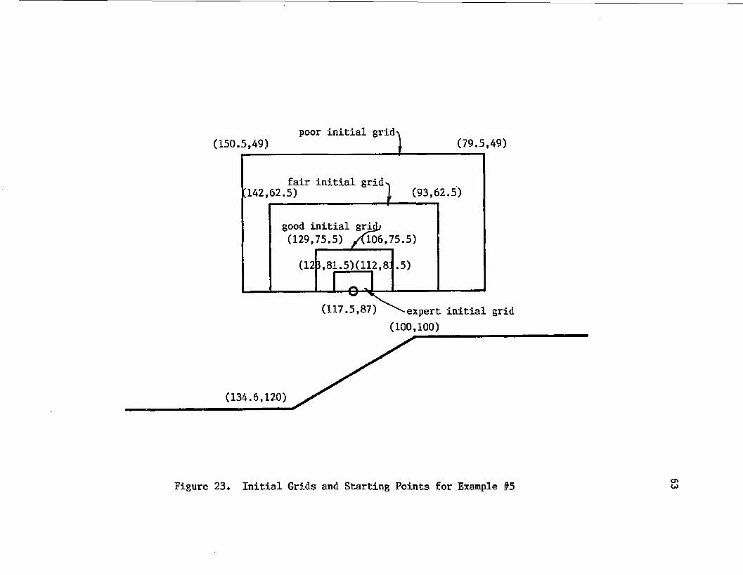
(79.5,49) (150.5,49)
,62.5) [142,62.5)
(129,75.5) Xl06,75.5)
(12
(117.5,87) ^•expert initial grid
(100,100)
(134.6,120)
Figure 23. Initial Grids and Starting Points for Example #5 Ot co

64
TABLE 14
PATTERN SEARCH RESULTS FOR EXAMPLE #5
Trial Starting
Point (ft)
Step Length Logic
Total No.. of Function Evaluations
Minimum F.S.
(x,y) Radius of Minimum (ft)
1 (150.5,49) A 69 0.781 (117.5,87),38
2 (150.5,49) B 86 0.781 (117.5,87),38
3 (79.5,49) A 53 0.781 (117.5,87),38
4 (79.5,49) B 70 0.781 (117.5,87),38
5 (142,62.5) A 50 0.781 (117.5,87),38
6 (142,62.5) B 63 0.781 (117.5,87),38
7 (93,62.5) A 47 0.781 (117.5,87),38
8 (93,62.5) B 54 0.781 (117.5,87),38
9 (129,75.5) A 45 0.781 (117.5,87),38
10 (129,75.5) B 44 0.781 (117.5,87),38
11 (106,75.5) A 42 0.781 (117.5,87),38
12 (106,75.5) B 38 0.781 (117.5,87),38
13 (123,81.5) A 41 0.781 (117.5,87),38
14 (123,81.5) B 34 0.781 (117.5,87),38
15 (112,81.5) A 42 0.781 (117.5,87),38
16 (112,81.5) B 31 0.781 (117.5,87),38

TABLE 15A
EFFECT OF STEP LENGTH LOGIC ON EFFICIENCY FOR EXAMPLE #5
Starting Step Length Average Number of Guess Logic Function Evaluations
Poor A 55 B 78
Fair A 49 B 59
Good A 44
B 41
Expert A 42
B 33
TABLE 15B
EFFECT OF EXPERTISE ON EFFICIENCY FOR EXAMPLE #5
Starting Guess
Poor
Fair
Good
Expert
Step Length Logic
B only
A-B average
A-B average
B only
Number of Function Evaluations
78
54
43
33

66
the critical tangent depth had been determined. Locating the critical
tangent depth is by far the most difficult and time-consuming part of
analyzing this type of problem.
4.6 Stepped Slope in Homogeneous Soil. The next example
studied was a stepped slope in homogeneous, cohesive soil. The slope
geometry is shown in Figure 24. For this type of slope profile, it is
not known initially whether the critical circle will be a toe circle or
a base circle. Safety factor contours were studied for both cases.
Figure 25 shows safety factor contours for slip circles which
are tangent to the firm stratum. The plot shows a fairly regular
contour pattern with a minimum value of 1.236.
Figure 26 shows safety factor contour for slip circles passing
through the upper toe of the slope. An examination of this figure
shows a regular contour pattern on the right side of the grid (above
the upper slope) having a minimum value of 1.718. However, the factor
of safety values gradually decrease as the corresponding circle centers
are chosen farther to the left side of the grid. This is an example of
a problem which does not have a single or unimodal minimum safety
factor value. Such a condition presents a problem in evaluating the
minimum safety factor using a pattern search procedure. If the
starting point for the search is chosen in the vicinity of the local
minimum (x,y) = (110,94), the search will converge to this point.
However, if the starting point is chosen farther to the left, in the
region of gradually decreasing safety factor values, the search will
not converge at all.

(140,115)
(120,115)
t = 120 pcf ff= 0 c = 500 psf
(160,130)
Figure 24. Example #6 - Benched Slope Face

68
min
Figure 25. Safety Factor Contours for Circles Tangent to Firm Stratum for Example #6

2.0 4.0 4.0 2.0
0.5
F.S. . = 1.718 mm
(local minimum)
upper toe of slope
Figure 26. Safety Factor Contours for Circles Passing Through Upper Toe for Example #6
CT> VO

70
4.7 Case Histories. A series of case histories was presented
by Krahn and Fredlund (1977) for the purpose of verifying the
University of Saskatchewan SLOPE program for slope stability (Fredlund,
1974). Krahn and Fredlund suggested that these problems could be used
as standard examples in future program verification studies. These
case histories are also suitable for use in verifying and comparing
search routines. However, it is very difficult to duplicate these
problems as they have been presented in the aforementioned paper due to
the extremely small scales used and incomplete or incorrect strength
parameter data. Therefore, the original references were consulted in
order to present accurate and complete information about each case
history. For convenience, complete information regarding each of these
nine problems is presented in Appendix A, together with sketches
showing the location of the critical circle.
4.8 Comparison of Grid and Pattern Search Results. The
results of the grid and pattern searches can be compared for the
various examples since they were found using identical procedures. i
These results are summarized in Table 16. An examination of this table
shows a general trend of decreasing efficiency with decreasing levels
of expertise. It can also be seen that a grid search requires many
more function evaluations than a pattern search for the same level of
expertise.
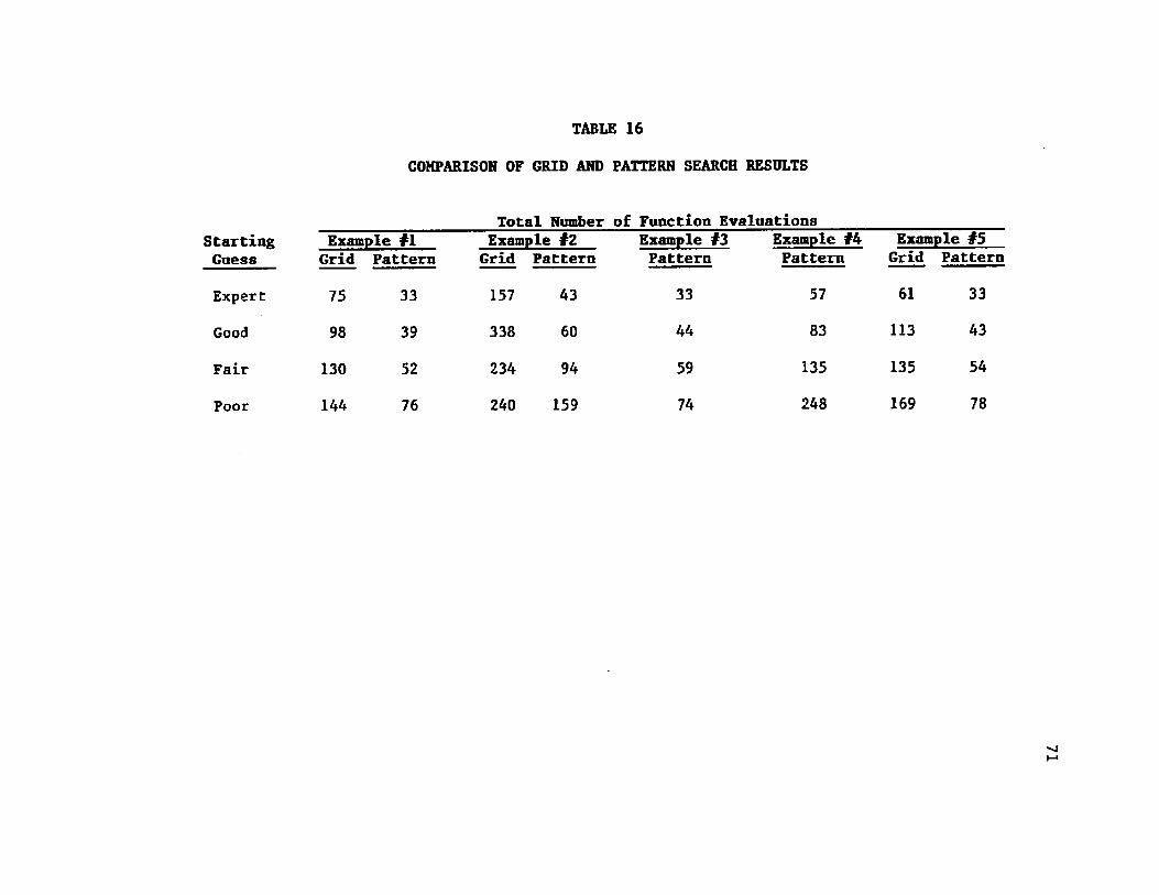
TABLE 16
COMPARISON OF GRID AND PATTERN SEARCH RESULTS
Total Number of Function Evaluations
Starting
Guess
Example #1
Grid Pattern
Example #2
Grid Pattern
Example #3 Pattern
Example #4
Pattern
Example #5
Grid Pattern
Expert 75 33 157 43 33 57 61 33
Good 98 39 338 60 44 83 113 43
Fair 130 52 234 94 59 135 135 54
Poor 144 76 240 159 74 248 169 78

CHAPTER 5
SUMMARY, CONCLUSIONS AND RECOMMENDATIONS
5.1 Summary. Slope stability analyses are commonly performed
using limit equilibrium methods. Many computer codes are available
that employ various limit equilibrium methods, as well as some type of
optimization strategy to locate the critical slip surface and
corresponding safety factor. A thorough search of literature and
commercially available computer codes revealed that all optimization
strategies currently in use in slope stability programs are direct
search methods, which are the most inefficient optimization techniques.
A wide range of slope stability problems, including several
published case histories, was presented. The problems are realistic
slope problems that can be easily duplicated. These problems will
serve as a basis for future comparative testing of optimization
algorithms as they are incorporated into slope stability analysis
programs. In this study, the efficiencies of two direct search
methods, the grid search and the pattern search, were evaluated using
the formulated set of problems.
5.2 Conclusions. Both the grid and the pattern search methods
are somewhat inefficient in locating the critical slip surface. This
is especially true for large-scale problems, such as Examples #2 and
#4, which require many function evaluations in the search for the
minimum safety factor. The grid and the pattern searches are largely
72

73
trial-and-error procedures for problems where the critical tangent
depth is unknown. In addition, the pattern search may produce
inaccurate results for problems such as stepped slopes, which may have
more than one local minimum safety factor. A grid search is the
preferred technique for these types of problems.
A comparison of the grid and the pattern search results reveals
that a grid search always requires more function evaluations than a
pattern search for the same level of expertise of the analyst.
Therefore, it can be concluded that the pattern search is generally
more efficient than the grid search.
The level of expertise of the analyst has a pronounced effect
on the efficiency of both the grid and the pattern search methods. A
poor choice of starting point combined with an inefficient step length
logic results in two to three times more function evaluations than an
expert starting point and logic for pattern searches. In grid
searches, using poor grid logic requires 1-1/2 to 3 times as many
function evaluations as an expert grid logic. The use of more advanced
optimization techniques in slope stability analysis would largely
eliminate the effect of user expertise.
5.3 Recommendations for Further Study. It is recommended that
a more efficient optimization algorithm be incorporated into one of the
existing slope stability analysis programs. This would greatly
increase the efficiency of slope stability analysis. The set of sample
problems presented here should be used as a basis of verification and
comparison of the resulting computer code.

APPENDIX A
NINE CASE HISTORIES
The first case history studied was the Congress Street Open Cut
in Chicago (Ireland, 1954). In consulting the original reference, it
was found that the single clay layer shown in the paper by Krahn and
Fredlund actually consisted of three separate layers having different
values of density and cohesion. A sketch of this example is shown in
Figure 27.
The second case history studied was the Brightlingsea slide,
which occurred in 1941 after a row of concrete blocks was placed on top
of a sea wall (Skempton and Golder, 1948). The configuration of this
problem is shown in Figure 28.
Another case history examined was the Seven Sisters' slide in
Western Canada (Peterson et al, 1957). A sketch of this example is
given in Figure 29.
A slip occurred in a railway cutting at Northolt in England in
1955 (Henkel, 1957). An effective stress analysis was performed. The
pore pressures were defined by the water level measured by piezometers
installed after the slip occurred. Figure 30 is a sketch of this
example.
Another case history presented by Krahn and Fredlund was the
Selset landslide (Skempton and Brown, 1961). This slide occurred in
74

75
APPENDIX A (Continued)
heavily overconsolidated clay. The slope . profile is shown in
Figure 31.
The Green Creek slide (Crawford and Eden, 1967) occurred in
Leda clay in Eastern Canada. An effective stress analysis was
performed using the pore pressure parameter ru to define the pore
pressures. Figure 32 shows the slope profile.
Three previously published example problems were also examined
by Krahn and Fredlund. These included an example from Bishop and
Morgenstern1s stability charts, Spencer's example problem, and
Morgenstern and Price's example problem. These examples are shown in
Figures 33 through 35. The Bishop-Morgenstern example was analyzed for
two pore pressure conditions, one with ru - 0 and the other with
ru = 0.45.
Figures 27 through 35 are intended to serve as references for
any future researchers who may wish to analyze these problems using
other, more advanced optimization techniques.

(X,Y) = (138,73)
(100,100) Elev. (ft.) J 100
y = no pcf
c = 0 psf = 30°
111 2f = 132 pcf c = 1420 psf
(130,117.6)
(124,117.6)
125
135 Y - 128 pcf c = 1060 psf = 0 (169.5,146.75)
•155 Stiff clay
Figure 27. Congress Street Open Cut
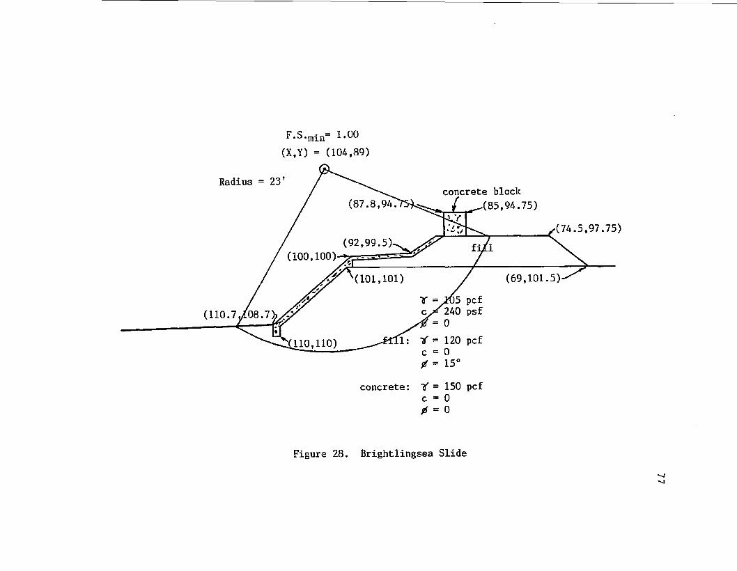
(X,Y) = (104,89)
Radius = 23' concrete block
/ .>(85,94.75) (87.8,94.
(74.5,97.75)
(92,99
(100,100)
(69,101.5) (101,101)
T = J V 5 pcf c 240 psf
1: ~)f = 120 pcf 110,110)
concrete: Y = 150 pcf c = 0
fS = 0
Figure 28. Brightlingsea Slide
•v!

(X,Y) = (121.7, 85.5)
(86,100) (100,100)
Elev. (ft.)
106 (37,114)
117.5 (58,114) (66,117.5 (126,117.5
133
c = 0. ff — 0
ff = 0
(2) r = 121 pcf c = 518 psf /! = 13°
Figure 29. Seven Sisters' Slide
03

79
F.S. . = 1.35 mm
(X,Y) = (153.7,62.3) Radius = 78.4'
(175,130), (177,131)
concrete wall
(177,136.5)'
piezometric line
107.5'
(175,137.5)
concrete: "jf = 150 pcf c = 2000 psf js = 35°
soil: Y = 125 pcf c'= 250 psf ff'= 20°
Figure 30. Northolt Slide
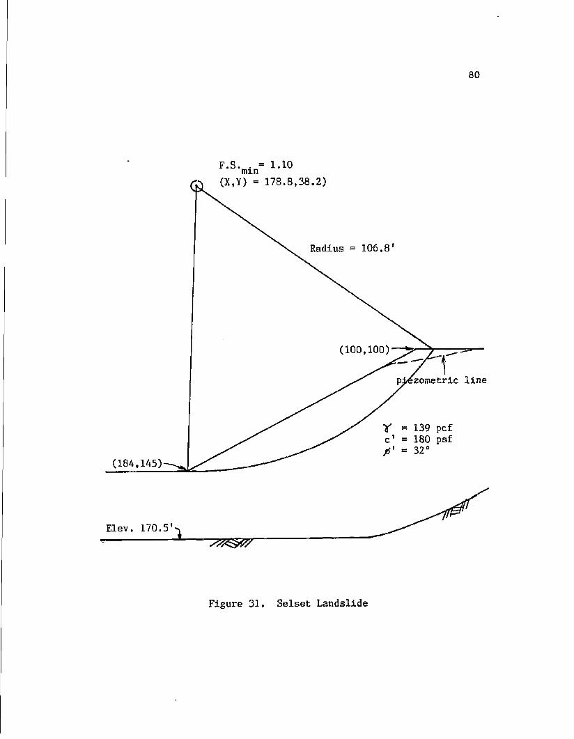
80
(X,Y) = 178.8,38.2)
Radius = 106.8'
(100,100)
piezometric line
y = 139 pcf
c' = 180 psf
Elev. 170.51
Figure 31. Selset Landslide

81
*min~ 9^?? F.S (X,YT'= (200.5,32.3)
Radius = 146.8'
(100,100)
t= 100 pcf c = 482 psf
20° (255,163)
Figure 32. Green Creek Slide
Case 1: r =0 u
F.S. = 1.87 (X,Y) = (350.4,-194.5) Radius = 397.7' Case 2:
(400,200)-^
r =0.45 u
(X.Y) = (315,-67.3) Radius - 280.8'
F.S. = 1.12
(100,100)
Y = 120 pcf
c = 300 psf fS = 25°
Figure 33. Bishop and Morgenstern's Example

82
(X,Y) = (304.4,-82.9) Radius = 282.91
(100,100)
Y = 120 pcf c = 240 psf / = 40e (300,200)
Figure 34. Spencer's Example Problem
F.S. = 1.80 (X,Y) = (246.6,1.6) Radius = 205.4'
(100,100)
Y= 120 pcf c = 1200 psf / = 20° (300,200)
Figure 35. Morgenstern and Price's Example Problem

APPENDIX B
STABR DATA FILES
83

PROBLEM #1: TOE CIRCLE 0 0 4 3 0 0 0 0 111.55 90.00 1 111.55 120. ,00
-90 100 100 100 160 200 100 100 100 100 160 200
111.55 120 120 120 160 200 300 120 120 120 160 200 1 500 0 120 2 4000 30 120

PROBLEM #2: BASE CIRCLE 0 1 4 3 0 0 0 0 126.00 75.00 1 160.00 -90 100 100 100 160 200 100 100 100 100 160 200 152.00 130 130 130 160 200 350 130 130 130 160 200
1 800 0 120 2 4000 30 120

PROBLEM #3: STRATIFIED SOIL 0 1 4 5 0 0 0 0 117.32 86.70 1 135.00 -200 100 100 100 130 135 150 200 100 100 100 100 130 135 150 200 134.64 120 120 120 130 135 150 200 550 120 120 120 130 135 150 200
1 500 0 120 2 0 30 120 3 500 0 120 4 4000 30 120

PROBLEM #4: BIRCH DAM 0 1 7 4 0 0 0 0 ISO 75 1 194 -200 100 100 100 100 194 194
44 100 100 100 100 194 194 72 100 100 100 157 169 194 86 100 100 100 157 157 194 100 100 100 100 157 157 194 500 157 157 157 157 157 194
1 1023 31 127 2 1629 18 127
3 1023 0 127

PROBLEM #5: CONTINUOUS COHESION VARIATION 0 1 4 2 0 2 0 0 117.30 86.00 1 124.00 -200 100 100 100 400 100 100 100 100 400
134.64 120 120 120 400 550 120 120 120 400 1-10 120 100 200 400 1700

PROBLEM #6: BENCHED SLOPE FACE 0 1 6 2 0 0 0 0 110 90 1 120 115 -100 100 100 100 130 100 100 100 100 130 120 115 115 115 130 140 115 115 115 130 160 130 130 130 130 300 130 130 130 130
1 500 0 120
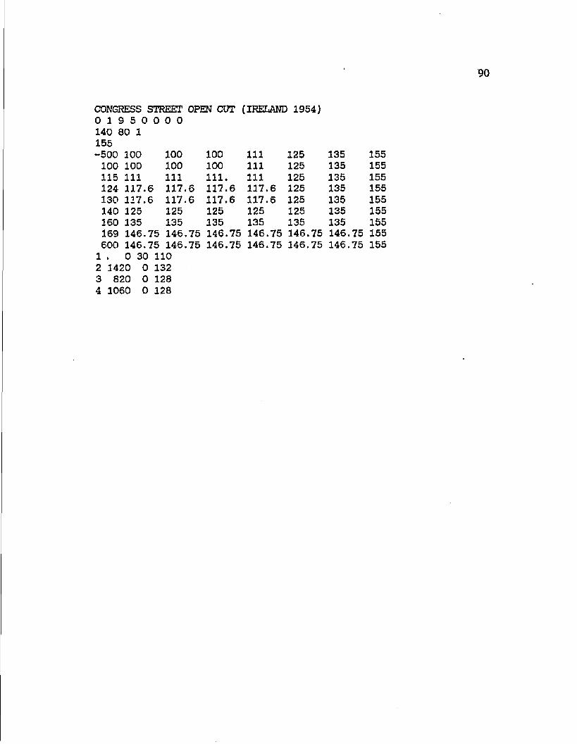
CONGRESS STREET OPEN CUT (IRELAND 1954) 0 1 9 5 0 0 0 0 140 80 1 155 500 100 100 100 111 125 135 155
100 100 100 100 111 125 135 155
115 111 111 111. 111 125 135 155 124 117.6 117.6 117.6 117.6 125 135 155
130 117.6 117.6 117.6 117.6 125 135 155
140 125 125 125 125 125 135 155
160 135 135 135 135 135 135 155 169 146.75 146.75 146.75 146.75 146.75 146.75 155
600 146.75 146.75 146.75 146.75 146.75 146.75 155
1 . 0 30 110 2 1420 0 132 3 820 0 128 4 1060 0 128

BRIGHTLINGSEA SLIDE {SKEMPTON & GOLDER, 1946) 0 1 1 6 4 0 0 0 0
100 90 1 112 69 101.5 101.5 101.5 101.5 101.5 140
74.5 97.75 97.75 97.75 97.75 101.5 140
84.9 97.75 97.75 97.75 97.75 101.5 140 85 94.75 94.75 94.75 98.1 101.5 140
87.8 94.75 94.75 94.75 98.1 101.5 140 87.9 97.75 97.75 97.75 98.1 101.5 140
88.5 97.75 97.75 97.75 98.75 101.5 140 92 99.5 99.5 99.5 100.2 101.5 140 99.9 100 100 100 100.2 101.5 140 100 100 100 100 101.5 101.5 140 101 101 101 101 101.5 101.5 140 109.9 108 108 108 108.5 108.5 140 110 108 108 108 110 110 140 110.7 108.7 108.7 108.7 110 110 140 110.8 108.7 108.7 108.7 108.7 108.7 140 150 114.4 114.4 114.4 114.4 114.4 140
1 0 0 150 2 0 15 120 3 240 0 105

SEVEN SISTERS SLIDE (PETERSON ET AL, 1957)
0 1 13 5 ] L 0 0 0
125 75 1 133 -25 117.5 117.5 117.5 117.5 117.5 117.5 133.
19 117.5 117.5 117.5 117.5 117.5 117.5 133.
27 114.0 114.0 114.0 114.0 114.0 117.5 133. 37 114.0 114.0 114.0 114.0 114.0 117.5 133.
58 108.0 108.0 108.0 108.0 114.0 117.5 133. 66 105.7 105.7 105.7 110.0 117.5 117.5 133.
74 103.4 103.4 103.4 106.0 117.5 117.5 133. 86 100.0 100.0 100.0 100.0 117.5 117.5 133. 100 100.0 100.0 100.0 100.0 117-5 117.5 133.
115 106.0 106.0 106.0 110.1 117.5 117.5 133.
126 110.3 110.3 110.3 117.5 117.5 117.5 133.
144 117.5 117.5 117.5 117.5 117.5 117.5 133.
250 117.5 117.5 117.5 117.5 117.5 117.5 133.
1 0 0 115 2 518 13 121 3 432 0 105 4 432 0 105 -25 106 19 106 27 106 37 106 58 106
66 106
74 107 86 109 100 111 115 114 126 117.5
144 117.5 250 117.5 0
0 0 0 0 0 0
0 0
0 0 0 0
0

NORTHOLT SLIDE (HENKEL, 1957) 0 1 8 3 1 0 0 0 130 40 1
141 -100 100 100 100 100 250 100 100 100 100 100 250
175 130 130 130 130 250 175.1 130 130 130 137. 5 250
177 131 131 131 136. 5 250
177.1 131 131 131 136. 5 250
177.2 132 132 132 132 250 300 132 132 132 132 250
1 2000 35 150 2 250 20 125 -100 107.5 100 107.5 175 134 175.1 137.5
177 136.5 177.1 132 177.2 132 300 132

SELSET LANDSLIDE (SKEMPTON & BROWN, 1961) 0 1 6 2 1 0 0 0 150 50 1 145 -50 100 100 100 147 67 100 100 100 147 100 100 100 100 164.2
112 106.4 106.4 106.4 170.5
184 145 145 145 170.5 400 145 145 145 170.5 1 180 32 139 -50 100 67 100 100 104 112 106.4 184 145 400 145

95
GREEN CREEK SLIDE (CRAWFORD & EDEN, 1967) 0 1 5 2 - 1 0 0 0 150 0 1 179 200 100 100 100 400 100 100 100 100 400
255 163 163 163 400 331 168 168 168 400 450 175.8 175.8 175.8 400
1 482 20 100 0.62

BISHOP AND MORGENSTERN EXAMPLE FOR RU 0 1 4 2 - 1 0 0 0 250 -100 1 203 -200 100 100 100 600 100 100 100 100 600 400 200 200 200 600 700 200 200 200 600
1 300 25 120 0

97
BISHOP AND MORGENSTERN EXAMPLE FOR RU = 0.45 0 1 4 2 - 1 0 0 0 250 -100 1 213.5 -200 100 100 100 600 100 100 100 100 600 400 200 200 200 600 700 200 200 200 600 1 300 25 120 0.45

SPENCER'S EXAMPLE 0 1 4 2 - 1 0 0 0 250 0 1 200 -300 100 100 100 500 100 100-100 100 500 300 200 200 200 500 600 200 200 200 500 1 240 40 120 0.5

MORGENSTERN & PRICE EKAMPLE 0 1 4 2 0 0 0 0 200 50 1 203.6 -300 100 100 100 500 100 100 100 100 500 300 200 200 200 500 600 200 200 200 500 1 1200 20 120

100
LIST OF REFERENCES
Awad, B. M. (1986, "Application of the Simplex Method to Slope Stability Analysis," M.S. Thesis, The University of Arizona, Department of Civil Engineering and Engineering Mechanics,
Tucson, Arizona.
Bailey, W. A. and J. T. Christian (1969), "ICES-LEASE-l; A Problem Oriented Language for Slope Stability Analysis," MIT Soil Mechanics Publication No. 235. Massachusetts Institute of Technology.
Baker, R. (1980), "Determination of the Critical Slip Surface in Slope Stability Computations," International Journal for Numerical and Analytical Methods in Geomechanics, Vol. 4, No. 4, pp. 333-359.
Boutrup, E. (1977), "Computerized Slope Stability Analysis for Indiana Highways, Vols. I and II," Joint Highway Research Project Report
Nos. JHRP-77-25 and JHRP-77-26, Engineering Experiment Station, Purdue University.
Boutrup, E. , Love 11, C. W., and R. A. Siegel (1979), "STABL2 - A Computer Program for General Slope Stability Analysis," Proceedings of the Third International Conference on Numerical
Methods in Geomechanics, pp. 747-757.
Carpenter, J. R. (1985), "PCSTABL4 User Manual," Joint Highway Research Project No. JHRP-85-7, Engineering Experiment Station, Purdue University.
Celestino, T. B. and J. M. Duncan (1981), "Simplified Search for Noncircular Slip Surfaces," Proceedings of the Tenth International Conference on Soil Mechanics and Foundation
Engineering, Vol. 3, pp. 391-394.
Chen, R. H. (1981), "Three-Dimensional Slope Stability Analysis," Joint Highway Research Project Report No. JHRP-81-17, Engineering Experiment Station, Purdue University.
Chugh, A. K. (1981), "User Information Manual, Slope Stability Analysis Program SSTAB2," Bureau of Reclamation, U. S. Department of the Interior.
Civilsoft (1976), Informational Brochure on SLOPE.

101
LIST OF REFERENCES (Continued)
Cornwell, L. W., Kocman, M. G., and M. F. Prosser (1980), "Computational Experience with Davidon's Least-Square Algorithm," Journal of Optimization Theory and Applications, Vol. 31, No. 1, pp. 27-39.
Crawford, C. B. and W. J. Eden (1967), "Stability of Natural Slopes in Sensitive Clay," Journal of Soil Mechanics Division, ASCE, Vol. 93, pp. 419-436.
Cross, J. P. (1982), "Slope Stability Program," Civil Engineering,
ASCE, Vol. 52, No. 10, pp. 71-74.
DeNatale, J. S. (1983), "On the Calibration of Constitutive Models by Multivariate Optimization, A Case Study: The Bounding Surface
Plasticity Model," Ph.D. Thesis, University of California at Davis, Department of Civil Engineering, 435 pp.
Duncan, J. M. and A. L. Buchignani (1975), "An Engineering Manual for Slope Stability Studies," University of California at Berkeley, Department of Civil Engineering.
Duncan, J. M. and S. G. Wright (1980), "The Accuracy of Equilibrium Methods of Slope Stability Analysis," Proceedings of the Third International Symposium on Landslides, Vol. 1, pp. 274-254.
Fredlund, D. G. (1974), "Slope Stability Analysis, User's Manual CD-4," Department of Civil Engineering, University of Saskatchewan.
Fredlund D. G. and J. Krahn (1977), "Comparison of Slope Stability Methods of Analysis," Canadian Geotechnical Journal, Vol. 14, pp. 429-439.
Fredlund, D. G., Krahn, J., and D. E. Pufahl (1981), "The Relationship Between Limit Equilibrium Slope Stability Methods," Proceedings of the Tenth International Conference on Soil Mechanics and Foundation Engineering, Stockholm, Vol. 3, pp. 409-416.
Fredlund, D. G. and J. D. Nelson (1985), "Course Notes: Slope Stability Analysis," Colorado State University, Geotechnical Engineering Program.
Geocomp Corporation (1986), Informational Brochure on GEOSLOPE.
Geo-Slope Programming Ltd. (1987), Informational Brochures on SLOPE-II and PC-SLOPE.
Geosoft (1986), Informational Brochures on STABRG and SL0P8RG.

102
LIST OF REFERENCES (Continued)
Henkel, D. J. (1975), "Investigations of Two Long Term Failures in London Clay Slopes at Wood Green and Northolt," Proceedings. Fourth International Conference on Soil Mechanics and Foundation Engineering, Vol. 2, pp 315-320.
Horn, J. A. (1960), "Computer Analysis of Slope Stability," Journal of the Soil Mechanics and Foundations Division, ASCE, Vol. 86, No. SM3, pp. 1-17.
Huang, Y. H. (1981), "User's Manual, REAME, A Computer Program for the Stability Analysis of Slopes," University of Kentucky, Institute for Mining and Minerals Research.
Huang, Y. H. (1983), Stability Analysis of Earth Slopes, Van Nostrand-Reinhold, New York.
Ireland, H. D. (1954), "Stability Analysis of the Congress Street Open Cut in Chicago," Geotechnique, Vol. 4, pp. 163-168.
Krahn, J. and D. G. Fredlund (1977), "Evaluation of the University of Saskatchewan Slope Stability Program," Road and Transportation Association of Canada Forum.
Lefebvre, G. (1971), "STABR User's Manual," University of California at Berkeley, Department of Civil Engineering.
Little, A. L. and V. E. Price (1958), "The Use of An Electronic Computer for Slope Stability Analysis," Geotechnique, Vol. 8, pp. 113-120.
Lovell, C. W., Sharma, S. S. and J. R. Carpenter (1984), "Slope Stability Analysis with STABL4," Joint Highway Research Project No. JHRP-84-19, Engineering Experiment Station, Purdue University.
Nelder, J. A. and R. Mead (1965), "A Simplex Method for Function Minimization, Computer Journal. Vol. 7, pp. 308-3131
Newman, E. E. (1985), personal communication.
Nguyen, V. U, (1985), "Determination of Critical Slope Failure Surfaces, Journal of Geotechnical Engineering. ASCE, Vol. Ill, No. 2, pp. 348-352.
Peterson, R. Iverson, N. L. and P. J. Rivard (1957), "Studies of Several Dam Failures on Clay Foundation," Proceedings, Fourth International Conference on Soil Mechanics and Foundation Engineering, Vol. 2, pp. 348-352.

103
LIST OF BEFERENCES (Continued)
Schiffman, R. L. (1972), "A Computer Program to Analyze the Stability of Slopes by Morgenstern's Method," Report No. 72-18. Department of Civil Engineering, University of Colorado at Boulder.
Schiffman, R. L. and D. M. Jubenville (1975), "User's Manual for MALE-1, Version 2-A: A Computer Program to Analyze the Stability of Slopes by Morgenstern's Method," GESA Report D-75-16, University of Colorado at Boulder.
Siegel, R. A. (1975b), "STABL User's Manual," Joint Highway Research Project Report No. JHRP-75-9, Engineering Experiment Station, Purdue University.
Siegel, R. A. (1975b), "STABL Uder's Manual," Joint Highway Research Project Report No. JHRP-75-90, Engineering Experiment Station, Purdue University.
Siegel, R. A., Kovack, W. D. and C. W. Lovell (1979), "New Method of Shear Surface Generation for Stability Analysis," Proceedings of the 29th Annual Highway Geology Symposium, pp. 295-312.
Skempton, A. W. and J. D. Brown (1961), "A Landslide in Boulder Clay at Selset, Yorkshire," Geotechnique, Vol. 11, pp. 280-293.
Skempton, A. W. and H. Q. Colder (1948), "Practical Examples of the = 0 Analysis of the Stability of Clays," Proceedings, Second
International Conference on Soil Mechanics and Foundation Engineering, Vol. 2, pp 63-70.
Swann, W. H. (1972), "Direct Search Methods," in Numerical Methods for Unconstrained Optimization (W. Murray, Ed.), Academic Press, London, U.K., pp. 13-28.
Taylor, D. W. (1948), Fundamentals of Soil Mechanics, John Wiley and Sons, New York.
Terzaghi, K. (1943), Theoretical Soil Mechanics, John Wiley and Sons, New York.
Von Gunten Engineering Software, Inc. (1985), Informational Brochure on SB-SLOPE.
Wright, S. G. (1974), "SSTABl - A General Computer Program for Slope Stability Analysis," Research Report No. GE-74-1, Department of Civil Engineering, University of Texas at Austin.