Initial Data for the Two-Body Problemof General Relativity

by

Gregory B. Cook

A dissertation submitted to the faculty of The University of North Carolina atChapel Hill in partial fulfillment of the requirements for the degree ofDoctor of Philosophy in the Department of Physics and Astronomy.

Chapel Hill

1990

Approved by:

Advisor

Reader

Reader

Reader

Reader

ii

c© 1990Gregory B. Cook

ALL RIGHTS RESERVED

iii

GREGORY B. COOK: Initial Data for the Two-Body Problem of General Relativity (Under the

direction of James W. York, Jr.)

ABSTRACT

The numerical study of Einstein’s equations is of considerable interest for both astrophysical

and purely theoretical reasons as it provides the only known avenue for the study of strong field,

highly relativistic gravitational interactions. Of particular interest is the geometrodynamic two-

body problem since the collision of two black holes is believed to be a strong source of gravitational

radiation. Before studying the dynamics of such collisions, one must first obtain complete initial-

data sets which represent two black holes in some initial configuration including non-vanishing linear

and angular momenta for each hole. A formalism for constructing such initial-data sets is reviewed.

Based on this formalism, computational techniques are developed which allow for the complete

specification of initial data describing both one and two black holes with individually specifiable

linear and angular momenta. In the case of two black holes, the initial data is constructed in

two separate, base coordinate systems. Bispherical coordinates are used to construct very accurate

initial-data sets. Cadez coordinates are also used because this coordinate system is most appropriate

for future work on the evolution of the initial data. A method for locating apparent horizons in the

initial-data sets is developed by posing the apparent-horizon equation as a boundary-value problem.

This method is applied to the single-hole, initial-data sets leading to a new understanding of the

physical content of these initial hypersurfaces. The physical content of the two-hole, initial-data sets

is also explored.

iv

To my wife, Tonya,and my parents,

for their love,support, and

understanding.

v

“If I have seen further it is bystanding on the shoulders of giants”

Sir Isaac Newton

vi

Acknowledgements

I gratefully acknowledge the assistance and encouragement I have received from my family,

friends, colleagues, and instructors. I am most especially thankful to my advisor, James W. York,

Jr., for his support, inspiration, and for many invaluable discussions. I have also benefitted greatly

from my interactions with Bernard Whiting, Charles Evans, Steve Christensen, Tsvi Piran, and

Steve Detweiler. In particular, I wish to thank Bernard Whiting for his seemingly endless patience

and enthusiasm.

I am grateful for the support I have received from the Department of Physics and Astronomy

at The University of North Carolina at Chapel Hill. Much of the computational work contained

in this dissertation has been performed on the Convex supercomputer run by the Academic Com-

puting Services at UNC–Chapel Hill and on the Cray Y-MP supercomputer at the North Carolina

Supercomputing Center. Financial support has been provided in part through National Science

Foundation grants PHY-8407492, PHY-8908741, and PHY-9001645.

vii

TABLE OF CONTENTS

Page

LIST OF TABLES . . . . . . . . . . . . . . . . . . . . . . . . . . . . . . . . . . . . . . . . . . . . . . . . . . . . . . . . . . . . . . . . . . . . . . . . . viii

LIST OF FIGURES . . . . . . . . . . . . . . . . . . . . . . . . . . . . . . . . . . . . . . . . . . . . . . . . . . . . . . . . . . . . . . . . . . . . . . . . ix

NOTATION AND CONVENTIONS . . . . . . . . . . . . . . . . . . . . . . . . . . . . . . . . . . . . . . . . . . . . . . . . . . . . . . . . xi

Chapter

1. Introduction . . . . . . . . . . . . . . . . . . . . . . . . . . . . . . . . . . . . . . . . . . . . . . . . . . . . . . . . . . . . . . . . . . . . . . . . . . . . 1

2. The (3 + 1) Decomposition . . . . . . . . . . . . . . . . . . . . . . . . . . . . . . . . . . . . . . . . . . . . . . . . . . . . . . . . . . . . . . 5

3. The Conformal and Transverse-Traceless Decompositions . . . . . . . . . . . . . . . . . . . . . . . . . . . . . . . . 16

4. The Conformal Imaging Approach . . . . . . . . . . . . . . . . . . . . . . . . . . . . . . . . . . . . . . . . . . . . . . . . . . . . . . . 20

5. Solutions of the Momentum Constraint . . . . . . . . . . . . . . . . . . . . . . . . . . . . . . . . . . . . . . . . . . . . . . . . . . 32

6. Inversion-Symmetric Extrinsic Curvature for Two Black Holes . . . . . . . . . . . . . . . . . . . . . . . . . . . 39

7. The Hamiltonian Constraint and Boundary Conditions . . . . . . . . . . . . . . . . . . . . . . . . . . . . . . . . . . . 45

8. Numerical Solution of the Hamiltonian Constraint for a Single, Axisymmetric Black Hole . 54

9. Axisymmetric Numerical Solutions of the Hamiltonian Constraint for Two Black Holes . . . 64

10. The Hamiltonian Constraint for Two Black Holes Using Cadez Coordinates . . . . . . . . . . . . . . 76

11. Apparent Horizons on Inversion-Symmetric Initial-Data Sets . . . . . . . . . . . . . . . . . . . . . . . . . . . . . 91

12. Apparent Horizons for a Single Black Hole with Linear or Angular Momentum . . . . . . . . . . . 96

13. Inversion-Symmetric, Single-Hole Initial-Data Sets . . . . . . . . . . . . . . . . . . . . . . . . . . . . . . . . . . . . . . . 105

14. Inversion-Symmetric, Two-Hole Initial-Data Sets . . . . . . . . . . . . . . . . . . . . . . . . . . . . . . . . . . . . . . . . . 113

15. Conclusion . . . . . . . . . . . . . . . . . . . . . . . . . . . . . . . . . . . . . . . . . . . . . . . . . . . . . . . . . . . . . . . . . . . . . . . . . . . . . . 126

Appendix A: The Multigrid Algorithm . . . . . . . . . . . . . . . . . . . . . . . . . . . . . . . . . . . . . . . . . . . . . . . . . . . . . . . 131

Appendix B: Numerical Solutions of the One-Hole Hamiltonian Constraint . . . . . . . . . . . . . . . . . . . 136

Appendix C: Numerical Solutions of the Two-Hole Hamiltonian Constraint in Bispherical Co-

ordinates . . . . . . . . . . . . . . . . . . . . . . . . . . . . . . . . . . . . . . . . . . . . . . . . . . . . . . . . . . . . . . . . . . . . . . . 152

Appendix D: Numerical Solutions of the Two-Hole Hamiltonian Constraint in Cadez Coordi-

nates . . . . . . . . . . . . . . . . . . . . . . . . . . . . . . . . . . . . . . . . . . . . . . . . . . . . . . . . . . . . . . . . . . . . . . . . . . . 173

References . . . . . . . . . . . . . . . . . . . . . . . . . . . . . . . . . . . . . . . . . . . . . . . . . . . . . . . . . . . . . . . . . . . . . . . . . . . . . . . . . . 194

viii

LIST OF TABLES

Table Page

8.1 Numerical solution of the model problem compared with the exact solution. . . . . . . . . . . . . . . 63

8.2 Energy and minimal surface mass for a single black hole with linear momentum. . . . . . . . . . . 63

8.3 Energy and minimal surface mass for a single black hole with angular momentum. . . . . . . . . 63

9.1 ADM energy of time-symmetric solutions of the Hamiltonian constraint at (80×80), (120×

120), and (160 × 160) mesh resolutions, Richardson extrapolated and compared with the

analytic solution for the ADM energy. β indicates the separation of the two holes. . . . . . . . . 73

9.2 Total energy and masses for two holes which are very far apart, the larger hole having linear

momentum P . The Extrinsic Curvature obeys the isometry condition with the plus sign.

(α = 20, β = 50) . . . . . . . . . . . . . . . . . . . . . . . . . . . . . . . . . . . . . . . . . . . . . . . . . . . . . . . . . . . . . . . . . . . . . . . . . 73

9.3 Total energy and masses for two holes which are very far apart, the larger hole having linear

momentum P . The Extrinsic Curvature obeys the isometry condition with the minus sign.

(α = 20, β = 50) . . . . . . . . . . . . . . . . . . . . . . . . . . . . . . . . . . . . . . . . . . . . . . . . . . . . . . . . . . . . . . . . . . . . . . . . . 74

9.4 Total energy and masses for two holes which are very far apart, the larger hole having

angular momentum S. The Extrinsic Curvature obeys the isometry condition with the

minus sign. (α = 20, β = 50) . . . . . . . . . . . . . . . . . . . . . . . . . . . . . . . . . . . . . . . . . . . . . . . . . . . . . . . . . . . . . 74

12.1 Minimal-surface mass and apparent-horizon mass for a hole with linear momentum P gen-

erated from A+ij . Also tabulated are the apparent-horizon amplitude H and its standard

deviation σ. . . . . . . . . . . . . . . . . . . . . . . . . . . . . . . . . . . . . . . . . . . . . . . . . . . . . . . . . . . . . . . . . . . . . . . . . . . . . . 104

ix

LIST OF FIGURES

Figure Page

4.1 Embedding diagram of time-symmetric, maximal slice of Schwarzschild geometry in isotropic

coordinates. . . . . . . . . . . . . . . . . . . . . . . . . . . . . . . . . . . . . . . . . . . . . . . . . . . . . . . . . . . . . . . . . . . . . . . . . . . . . . 23

4.2 Time-symmetric, maximal slice of Kruskal space-time, labeled in isotropic coordinates and

showing “top” and “bottom” sheets in the two different universes. . . . . . . . . . . . . . . . . . . . . . . . . 24

4.3 Initial slice topologies for two black holes. a) Topology of an N + 1 sheeted manifold. b)

Topology of a two-sheeted manifold. . . . . . . . . . . . . . . . . . . . . . . . . . . . . . . . . . . . . . . . . . . . . . . . . . . . . . 25

8.1 Computational mesh and “virtual” boundary points. . . . . . . . . . . . . . . . . . . . . . . . . . . . . . . . . . . . . . 59

9.1 Two-hole background space parameterization and solution domain. . . . . . . . . . . . . . . . . . . . . . . . 64

10.1 Cadez coordinates near the two holes showing important coordinate lines and the three

region nature of the coordinate system. . . . . . . . . . . . . . . . . . . . . . . . . . . . . . . . . . . . . . . . . . . . . . . . . . . 79

10.2 Eight-point differencing molecule used for singular point. . . . . . . . . . . . . . . . . . . . . . . . . . . . . . . . . . 85

11.1 An apparent horizon S intersecting the initial-data surface Σ. nµ is the timelike unit normal

vector for the initial-data surface and sµ is the outward pointing spacelike unit normal to

the apparent horizon. . . . . . . . . . . . . . . . . . . . . . . . . . . . . . . . . . . . . . . . . . . . . . . . . . . . . . . . . . . . . . . . . . . . . 92

12.1 Apparent-horizon function h(θ) for a hole with linear momentum P/a = 10 generated by

A+ij . . . . . . . . . . . . . . . . . . . . . . . . . . . . . . . . . . . . . . . . . . . . . . . . . . . . . . . . . . . . . . . . . . . . . . . . . . . . . . . . . . . . . . 104

13.1 Energy and velocity for a boosted black hole with linear momentum P generated from the

extrinsic curvature A+ij . . . . . . . . . . . . . . . . . . . . . . . . . . . . . . . . . . . . . . . . . . . . . . . . . . . . . . . . . . . . . . . . . . . 108

13.2 Energy and velocity for a boosted black hole with linear momentum P generated from the

extrinsic curvature A−ij . . . . . . . . . . . . . . . . . . . . . . . . . . . . . . . . . . . . . . . . . . . . . . . . . . . . . . . . . . . . . . . . . . . 108

13.3 Energy of a spinning black hole with angular momentum S. . . . . . . . . . . . . . . . . . . . . . . . . . . . . . . 109

13.4 The location of the top and bottom apparent horizons (for data sets generated from A+ij)

and the minimal surface in the conformal background space. Also plotted are the spatial

projections of various “outgoing” null vectors with negative expansion. . . . . . . . . . . . . . . . . . . . 110

13.5 The location of the apparent horizons (for data sets generated from A+ij) and the minimal

surface illustrated on an embedding diagram of the geometry. . . . . . . . . . . . . . . . . . . . . . . . . . . . . 111

x

14.1 (a) total energy, (b) separation, (c) maximum radiation energy, and (d) maximum radiation

efficiency for two holes with linear momenta P aligned anti-parallel to each other and

generated by an inversion-symmetric extrinsic curvature obeying the isometry condition

with a plus sign. . . . . . . . . . . . . . . . . . . . . . . . . . . . . . . . . . . . . . . . . . . . . . . . . . . . . . . . . . . . . . . . . . . . . . . . . 116

14.2 (a) total energy, (b) separation, (c) maximum radiation energy, and (d) maximum radiation

efficiency for two holes with linear momenta P aligned parallel to each other and generated

by an inversion-symmetric extrinsic curvature obeying the isometry condition with a plus

sign. . . . . . . . . . . . . . . . . . . . . . . . . . . . . . . . . . . . . . . . . . . . . . . . . . . . . . . . . . . . . . . . . . . . . . . . . . . . . . . . . . . . . 117

14.3 (a) total energy, (b) separation, (c) maximum radiation energy, and (d) maximum radiation

efficiency for two holes with linear momenta P aligned anti-parallel to each other and

generated by an inversion-symmetric extrinsic curvature obeying the isometry condition

with a minus sign. . . . . . . . . . . . . . . . . . . . . . . . . . . . . . . . . . . . . . . . . . . . . . . . . . . . . . . . . . . . . . . . . . . . . . . . 119

14.4 (a) total energy, (b) separation, (c) maximum radiation energy, and (d) maximum radiation

efficiency for two holes with linear momenta P aligned parallel to each other and generated

by an inversion-symmetric extrinsic curvature obeying the isometry condition with a minus

sign. . . . . . . . . . . . . . . . . . . . . . . . . . . . . . . . . . . . . . . . . . . . . . . . . . . . . . . . . . . . . . . . . . . . . . . . . . . . . . . . . . . . . 120

14.5 (a) total energy, (b) separation, (c) maximum radiation energy, and (d) maximum radiation

efficiency for two holes with angular momenta S aligned anti-parallel to each other and

generated by an inversion-symmetric extrinsic curvature obeying the isometry condition

with a minus sign. . . . . . . . . . . . . . . . . . . . . . . . . . . . . . . . . . . . . . . . . . . . . . . . . . . . . . . . . . . . . . . . . . . . . . . . 122

14.6 (a) total energy, (b) separation, (c) maximum radiation energy, and (d) maximum radiation

efficiency for two holes with angular momenta S aligned parallel to each other and generated

by an inversion-symmetric extrinsic curvature obeying the isometry condition with a minus

sign. . . . . . . . . . . . . . . . . . . . . . . . . . . . . . . . . . . . . . . . . . . . . . . . . . . . . . . . . . . . . . . . . . . . . . . . . . . . . . . . . . . . . 123

14.7 Comparison of the scaled total energy for two holes with angular momenta S aligned anti-

parallel and parallel to each other showing the spin-spin interaction. . . . . . . . . . . . . . . . . . . . . . 124

xi

Notation and Conventions

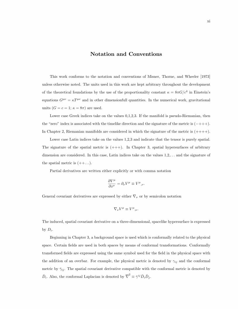
This work conforms to the notation and conventions of Misner, Thorne, and Wheeler [1973]

unless otherwise noted. The units used in this work are kept arbitrary throughout the development

of the theoretical foundations by the use of the proportionality constant κ = 8πG/c4 in Einstein’s

equations Gµν = κTµν and in other dimensionfull quantities. In the numerical work, gravitational

units (G = c = 1; κ = 8π) are used.

Lower case Greek indices take on the values 0,1,2,3. If the manifold is pseudo-Riemanian, then

the “zero” index is associated with the timelike direction and the signature of the metric is (−+++).

In Chapter 2, Riemanian manifolds are considered in which the signature of the metric is (++++).

Lower case Latin indices take on the values 1,2,3 and indicate that the tensor is purely spatial.

The signature of the spatial metric is (+++). In Chapter 3, spatial hypersurfaces of arbitrary

dimension are considered. In this case, Latin indices take on the values 1,2,. . . and the signature of

the spatial metric is (++. . .).

Partial derivatives are written either explicitly or with comma notation

∂V µ

∂xν= ∂νV

µ ≡ V µ,ν .

General covariant derivatives are expressed by either ∇ν or by semicolon notation

∇νV µ ≡ V µ;ν .

The induced, spatial covariant derivative on a three-dimensional, spacelike hypersurface is expressed

by Di.

Beginning in Chapter 3, a background space is used which is conformally related to the physical

space. Certain fields are used in both spaces by means of conformal transformations. Conformally

transformed fields are expressed using the same symbol used for the field in the physical space with

the addition of an overbar. For example, the physical metric is denoted by γij and the conformal

metric by γij . The spatial covariant derivative compatible with the conformal metric is denoted by

Di. Also, the conformal Laplacian is denoted by ∇2 ≡ γijDiDj .

xii

Beginning in Chapter 4, spatial hypersurfaces which are constructed from manifolds containing

multiple “throats” or “holes” are considered. To indicate that a certain quantity is associated with

a specific hole, a lower case Greek index will be used. This is not a tensor index and its position

(up or down) is not significant. Tensor indices on these fields will be denoted using lower case Latin

indices since the fields are purely spatial.

Chapter 1: Introduction

The most widely accepted theory of the dynamics of classical gravitational interactions is the

theory of general relativity.* Proposed in 1916 by Albert Einstein, it forever changed our under-

standing of what gravity is and how it shapes our universe. The Newtonian view of gravity held it as

a force which acted through space and affected the course of matter through time. General relativity,

on the other hand, intimately links gravity with space and time by considering our universe as a

four-dimensional, pseudo-Riemannian manifold in which curvature in the space-time metric is the

manifestation of gravity.

Any theory of gravity is meant to describe the basic attractive interaction between massive

objects. The most fundamental dynamical interaction in any theory of gravity, then, is that between

two massive bodies. The two-body problem, from the point of view of Newtonian gravity, is well

understood. One can easily specify the masses, initial positions, and initial velocities of two point

particles and determine the time development of this initial configuration. The Newtonian equations

of motion for two massive point particles are exactly solvable. The analogous problem in general

relativity is not well understood.

The two-body problem of general relativity has been studied through many approximations.

The most familiar general relativistic solution to the two-body problem is the prediction of the

precession of the perihelion of an orbit. This is one example of an approximate solution which can

be obtained by assuming the gravitational field is weak. The general formalisms for obtaining such

solutions are known as the post-Newtonian and the post-Minkowskian approximation methods. The

collision of two Schwarzschild black holes has been studied, analytically, in the limit that one hole is

much smaller than the other so that it can be treated as a perturbation. There are certainly other

approximation methods for studying the two-body problem, but to date there are no known exact

or approximate analytic solutions to the problem of the strong field, relativistic interaction of two

massive bodies. Currently, the only known avenue for the investigation of these very interesting

situations is through the use of numerical techniques.

* Here, the term classical gravitation is meant to imply that in any problem to which general relativity is applied;the length, energy, and time scales are in the classical and not in the quantum regime.

2

An important consequence of the theory of general relativity is the production and propagation

of gravitational waves from dynamic gravitational configurations. Violent astrophysical events, such

as binary coalescence, will most likely be the strongest emitters of gravitational radiation. It is

believed that the detection and study of gravitational waves from these events will play an important

role in the understanding of such astrophysical phenomena. Because of this, a vigorous experimental

and theoretical investigation of methods for detecting gravitational waves is under way, stemming

from the early 1960s. The latest generation of detectors, known as Laser Interferometer Gravity

Wave Observatories (LIGOs), should be sensitive enough to have a high probability of detecting

gravitational waves. As of this writing, the National Science Foundation has included funding for

the LIGOs in the budget for fiscal year 1991, with an estimated four-year expenditure of $192 million.

The numerical study of Einstein’s equations has been under exploration since the early 1960s

(Hahn and Lindquist [1964]), and has been vigorously pursued since the mid 1970s. To quote Thorne

[1987], “The effort may absorb almost as many person-years as the development of gravitational-wave

detectors; but it will be well worthwhile: the payoffs will include the ability to compute in detail the

waveforms from the strongest gravity-wave sources in the universe, such as the spiraling together and

coalescence of two black holes—waveforms that will be crucial to the interpretation of gravity-wave

observations and to their use in strong-field, highly dynamical tests of general relativity.”

Considering the statements above, I feel that the study of the fully relativistic, strong-field,

two-body problem is of prime concern to the fields of classical general relativity and relativistic

astrophysics. There are essentially two avenues for pursuing this problem. The first involves a study

of the collision of two compact material objects such as neutron stars. Efforts in this line have been

made by Evans [1986b], [1987]. The second avenue involves the purely geometrodynamic collision of

two black holes. In this case, one of the pioneering numerical relativistic calculations was undertaken

by Smarr [1977] in exploring the head-on collision of two black holes. In the first case, matter is

present in quantities sufficient to produce strong gravitational fields. The matter fields evolve in a

tightly coupled manner with the gravitational field and, given the proper initial conditions, produce

a collision. A numerical calculation of this kind involves solving the full Einstein field equations and

the relativistic hydrodynamic equations on a simply connected topology. In the case of a purely

geometrodynamic collision, only the Einstein field equations need to be solved since the space-time

is considered to contain no matter. On the other hand, to support the strong gravitational fields,

we must use non-trivial topologies. With this second approach, the interaction of black holes can

be modeled and it is the interaction of two black holes which is the closest relativistic analog of the

Newtonian two-body problem for point masses.

3

The aim of this dissertation is to advance the understanding of the relativistic two-body problem

for black holes. A great deal of theoretical and computational work has already been done toward this

goal. Misner [1963], Lindquist [1963], and Brill and Lindquist [1963] found a set of analytic solutions

to the initial-value equations of general relativity which represented any number of black holes

initially at rest in a vacuum. Hahn and Lindquist [1964] and Cadez [1971] made early attempts to

evolve this initial data numerically but met with little success. Besides the computational resources

available, the major hindrance in these early calculations stemmed from a poor formal understanding

of both the initial-value problem and the dynamics and kinematics of the Einsteinian evolution

equations. York [1971], [1972], [1973a], [1979], O Murchada and York [1973], [1974a], [1974b],

[1974c] and Smarr and York [1978a], [1978b] made many advances in the theoretical understanding

of these problems and Smarr et al. [1976] and Smarr [1977] performed the first successful numerical

simulation of black hole collisions. Smarr’s calculations started with Misner’s initial data for two

black holes initially at rest and followed the holes as they fell into a head-on collision while emitting

gravitational radiation.

In order to simulate more realistic and interesting situations, it is necessary to specify initial

conditions which represent black holes with non-zero linear and angular momenta. York [1979],

Bowen [1979b], and Bowen and York [1980] developed a formalism for specifying the initial data for

a single black hole with non-zero linear and angular momenta. Many authors, (York and Piran [1982],

Choptuik [1982], Rauber [1986], and Cook and York [1990]), have studied single-hole, axisymmetric

initial-data sets using numerical methods based on this framework. The formalism employed for

prescribing the initial data for a single hole was generalized to allow for multiple black holes by

Kulkarni et al. [1983], York [1984], and Kulkarni [1984]. In principle, this method allows for the

individual specification of linear and angular momenta for each hole permitting one, for example, to

specify initial data for the spiralling coalescence of two black holes. Based on this formal approach,

Bowen, Rauber, and York [1984] detailed an approach for specifying the initial data for two black

holes with axisymmetric parallel spins. Rauber [1986] attempted to solve numerically for the data

sets based on this approach but was unable to generate any complete solutions.

We call the collection of the formalisms and assumptions described in the papers listed above the

conformal imaging technique. This approach is not unique and in fact Thornburg [1987] has found

numerical solutions, based on an alternate set of assumptions, to the initial value equations for two

black holes with axisymmetric linear and angular momenta. I feel, however, that the conformal

imaging approach will be a more fruitful approach and proceed in this dissertation to describe and

4

examine solutions to the initial-value equations, based on the conformal imaging approach, which

describe two black holes with axisymmetric linear and angular momenta.

In the chapters which follow, I begin by outlining the conformal imaging approach. This consists

of the (3+1) decomposition of Einstein’s equations, York’s conformal decomposition of the constraint

equations, and the choice of the topology of the initial-data slice along with the isometry condition

imposed on this slice and its consequences for the initial-value equations. Next, I will discuss the

analytic solutions to the momentum constraint equations for a single black hole, the formal extension

to multiple black holes, and my algorithm for evaluating this formal solution. The following chapters

will discuss the numerical techniques used, and the solutions found, for the case of a single black

hole with linear or angular momentum and for two black holes with axisymmetric linear or angular

momenta. One aspect of initial-data slices which has not been explored sufficiently is the existence

and location of apparent horizons. I will proceed with a description of the consequences of the

conformal imaging approach on the existence and location of these apparent horizons and detail

their properties for the single black hole initial-data sets. Finally, I will conclude with some remarks

on future work.

Chapter 2: The (3 + 1) Decomposition

Einstein’s equations in full covariant form are a set of coupled partial differential equations, the

solution of which is a metric gµν that represents the full pseudo-Riemannian geometry of a space-

time. This metric is not a dynamical object in that it does not change in time. On the contrary,

the metric represents the geometry at all times just as the metric of a two-sphere represents the

geometry of that two-sphere at all points on the sphere. In order for Einstein’s equations to reveal

their dynamical nature, we must break the full, four-dimensional covariance and exploit the special

nature of time. One method of doing this is the (3+1) decomposition of Arnowitt, Deser, and Misner

(ADM) [1962]. The idea behind the (3 + 1) decomposition is to divide space-time into a sequence

of “instants” of time. Each instant of time holds an “instantaneous state” of the gravitational

field which dynamically evolves from instant to instant. Formally, the (3 + 1) decomposition allows

Einstein’s equations to be posed as a Cauchy problem (cf. Choquet-Bruhat and York [1980]). In

the remainder of this chapter, I will present the (3 + 1) splitting of Einstein’s equations based

largely on York [1979], Bowen [1979b], and Evans [1984]. The Einstein equations will be split into

constraint equations which are solved to give the initial data for a gravitational configuration on

some initial slice, and evolution equations which describe the dynamics of general relativity and take

the gravitational configuration from slice to slice.

Consider a 4-dimensional space with metric gµν having signature (ε+ ++), where ε = ±. (For

generality, we consider both pseudo-Riemannian (ε = −) and Riemannian (ε = +) spaces. In

this work, we will only be concerned with pseudo-Riemannian space-times, though it is useful to

keep track of where the special nature of time affects the equations. Also, the generality is useful

considering the importance of Euclidian methods in other areas of relativity.) The space is assumed

to be globally hyperbolic (ε = − case) so that it can be foliated by a family of 3-dimensional

hypersurfaces Σ that fills the space V . Let τ be a scalar function such that the level surfaces of τ

are the hypersurfaces Σ. If the space can contain a foliation Σ, then the foliation can be described

by a closed one-form Ω∼ = Ωµe∼µ where

dΩ∼ = 0 or ∇[µΩν] = 0 (2.1)

6

and e∼µ is a general basis of forms. Since Ω is closed, it must satisfy

Ω∼ = dτ or Ωµ = ∇µτ. (2.2)

The lapse function α defines the norm ‖Ω‖ by means of the space-time metric gµν

‖Ω‖ = gµνΩµΩν = gµν∇µτ∇ντ = εα−2, (2.3)

so the normalized one-form ω∼ associated with Σ is given by

ωµ ≡ αΩµ = α∇µτ. (2.4)

The minus sign for pseudo-Riemannian space-times and the strictly positive nature of α guarantee

that the hypersurfaces defined by ω∼ will be spacelike everywhere. The unit normal vector of a slice

is given by

nν = εgµνωµ, (2.5)

so that nµωµ = 1 (and so that it is timelike nµnµ = −1 for ε = −).

The spatial metric γµν induced by gµν onto a slice Σ is given by

γµν = gµν − εnµnν = gµν − εωµων , (2.6)

and the inverse spatial metric is given by

γµν = gµαgνβγαβ = gµν − εnµnν . (2.7)

Each index on a tensor can be decomposed into two pieces, one which is purely spatial and lies

entirely in the surface Σ and one which is entirely normal to the surface. The projection operator

⊥, which projects free indices into the slice Σ, is defined as

⊥µν ≡ γµν = δµν − εnµnν ; ⊥µνnµ = 0. (2.8)

Similarly, the projection operator N , which projects free indices normal to the slice, is defined as

Nµν ≡ εnµnν = δµν −⊥

µν ; Nµ

ν nµ = nν . (2.9)

Note that ⊥ and N are idempotent projection operators since

⊥µρ⊥ρν = ⊥µν and ⊥µµ = 3, (2.10)

7

and

NµρN

ρν = Nµ

ν and Nµµ = 1. (2.11)

Given the spatial metric on a hypersurface Σ, we can define a spatial covariant derivative Dµ

which is compatible with the metric γµν and which, acting upon spatial tensors, produces spatial

tensors. This operator is defined by taking the full covariant derivative of a tensor and projecting all

free indices into the hypersurface. Letting ⊥ with no indices represent the product of n projection

operators, one for each free index on the object upon which it is acting, then

DµTα···β

ρ···σ ≡⊥ ∇µTα···βρ···σ

= ⊥νµ⊥ακ · · · ⊥

βλ⊥

ζρ · · · ⊥

ξσ∇νTκ···λζ···ξ.

(2.12)

It is easily seen that the spatial covariant derivative is compatible with the spatial metric

Dαγµν = ⊥βα⊥ρµ⊥

σν∇β (gρσ − εnρnσ) = 0. (2.13)

The requirement that the spatial covariant derivative acts only on spatial tensors is required in order

for Leibnitz’s rule to hold.

Dα (V µWµ) = ⊥βα∇β (V µWµ)

= ⊥βαV µ(⊥ρµ +Nρ

µ

)∇βW ρ +⊥βαWµ

(⊥µρ +Nµ

ρ

)∇βV ρ

= V µDαWµ +WµDαVµ +⊥βα

(V µNρ

µ∇βW ρ +WµNµρ∇βV ρ

) (2.14)

which satisfies Leibnitz’s rule only if V µ and Wµ are purely spatial, i.e. NρµV

µ = 0 and NµρWµ = 0.

A slice Σ has “intrinsic” curvature defined in the standard way by the commutation of covariant

derivatives. If NµρWµ = 0, then

[Dµ, Dν ]W σ = W ρ(3)Rρσνµ and nρ

(3)Rρσνµ = 0. (2.15)

Here, (3)Rρσνµ is the spatial Riemann tensor for the hypersurface Σ, as opposed to (4)Rρσνµ which

is the Riemann tensor for the full 4-dimensional space. Since Σ is an embedded hypersurface, the

shape of the slice in the full space or the “extrinsic” curvature of the slice is also of interest. The

extrinsic curvature of a hypersurface is related to the projection of the gradient of the surface normal

vector field. This naturally consists of two parts: the symmetric part Θµν , known as the “strain”,

and the antisymmetric part ωµνˇ

, known as the “twist”

Θµν ≡⊥ ∇(µnν) and ωµν

ˇ≡⊥ ∇[µnν]. (2.16)

Since the vector field nµ is surface-forming by definition (dΩ∼ = 0), it is easy to show that

ω ∧ dω = 0 or ω[µ∇νωσ] = 0. (2.17)

8

It follows immediately that n[µ∇νnσ] = 0. By contracting with nµ and projecting the remaining

free indices we find

⊥(nµn[µ∇νnσ]

)=

13⊥(−∇[νnσ] +

12nµ(nσ∇[µnν] − nν∇[µnσ]

))= −1

3⊥ ∇[νnσ] = 0.

(2.18)

And so the twist vanishes. The extrinsic curvature of the slice, Kµν , is defined as minus the strain

Kµν ≡ −Θµν = − ⊥ ∇(µnν). (2.19)

Note that the choice of the minus sign is a convention. The extrinsic curvature can be expressed in

a more convenient form by expanding the gradient of the unit normal

∇µnν = δαµδβν∇αnβ =

(⊥αµ + εnαnµ

) (⊥βν + εnβnν

)∇αnβ

=⊥ ∇µnν + εnµ ⊥ aν(2.20)

where the acceleration of the unit normal, aµ, has been used

aµ = nν∇νnµ. (2.21)

Note that the acceleration is purely spatial since its contraction with the unit normal vanishes. This

follows from the identity

∇µ (nνnν) = 2nν∇µnν = 0. (2.22)

Since the acceleration is spatial, ⊥aµ = aµ and we find

∇µnν = −Kµν + εnµaν . (2.23)

Since the extrinsic curvature is symmetric, we can express it as

Kµν = −∇(µnν) + εn(µaν) (2.24)

from which it is easily seen that the extrinsic curvature is also purely spatial. From this and the

definition of the Lie derivative, it follows that

Kµν =⊥ Kµν =⊥(−∇(µnν) + εn(µaν)

)= − ⊥ ∇(µnν)

= −12⊥ £ngµν .

(2.25)

Alternatively, if we look at the Lie derivative of the spatial metric, we find

£nγµν = £n (gµν − εnµnν)

= 2(∇(µnν) − εn(µaν)

)= −2Kµν .

(2.26)

9

Since the unit normal is a timelike vector, the Lie derivative, alone nµ, of the spatial metric (and

thus the extrinsic curvature) is related to the “velocity” of the spatial metric on the slice Σ.

Given a slice Σ in space-time, its complete geometry is described by its spatial metric and

extrinsic curvature. Thus, the spatial metric and extrinsic curvature represent the “instantaneous

state” of the gravitational field and are the dynamical quantities which will be followed to explore

the evolution of a gravitational field. In order that a foliation of slices, Σ, can fit into the higher

dimensional space, they must satisfy certain conditions known as the Gauss-Codazzi-Ricci conditions.

These are obtained by taking all of the possible projections of the Riemann tensor of the full space.

We can spatially project all of the indices of the Riemann tensor into the hypersurface, contract one

index with the unit normal and spatially project the remaining three free indices, and finally we can

contract two of the indices with unit normals and project the remaining two. All other combinations

are identically zero by the symmetries of the Riemann tensor. To explore these, consider first

DµDνV ρ =⊥ ∇µ (⊥ ∇νV ρ)

=⊥ ∇µ∇νV ρ+ ⊥ (∇νV σ)(∇µ⊥σρ

)+ ⊥ (∇σV ρ) (∇µ⊥σν ) .

(2.27)

If we now expand the gradient of the projection operator, we find

∇σ⊥µν = εnνKσµ − nνnσaµ + εnµKσν − nµnσaν . (2.28)

Combining (2.27) and (2.28), we find

DµDνV ρ =⊥ ∇µ∇νV ρ + ε ⊥ KµρKνσV σ + ε ⊥ Kµνn

σ∇σV ρ. (2.29)

Then, using the definition of the Riemann tensor in terms of the commutation of covariant derivatives

(2.15), we get

(3)RµνρσV σ =⊥ (4)Rµνρ

σV σ + ε ⊥ KµρKνσV σ − ε ⊥ KνρKµ

σV σ, (2.30)

which gives us the form of the fully projected Riemann tensor known as Gauss’ equation:

⊥ (4)Rµνρσ = (3)Rµνρσ − εKµρKνσ + εKµσKνρ. (2.31)

If we contract one index on the Riemann tensor with the unit normal and project the rest, we

find

⊥ (4)Rµνρσnσ =⊥ (∇µ∇νnρ −∇ν∇µnρ) . (2.32)

To simplify this, consider one of the terms on the right-hand side.

⊥ ∇µ∇νnρ =⊥ ∇µ (−Kνρ + εnνaρ) = −DµKνρ + ε ⊥ (aρ∇µnν)

= −DµKνρ − εaρKµν .(2.33)

10

It follows, then, that the singly contracted, projected Riemann tensor gives

⊥ (4)Rµνρσnσ = DνKµρ −DµKνρ, (2.34)

which is known as Codazzi’s equation.

Note that Gauss’ and Codazzi’s equations depend only on the spatial metric, extrinsic curvature,

and their spatial derivatives. This implies that the Gauss-Codazzi equations represent integrability

conditions which the spatial metric and extrinsic curvature must satisfy in order for any given slice to

fit into the full space. These equations will be directly related to the constraints of general relativity.

Finally, explicit calculation shows

£nKµν = nρ∇ρKµν +Kµρ∇νnρ +Kρν∇µnρ

= (4)Rµρνσnρnσ −KµρKν

ρ + εKµρnνaρ −∇µaν + εaµaν + εnµn

ρ∇ρaν .(2.35)

Projecting this into the hypersurface yields

⊥ (4)Rµρνσnρnσ =⊥ £nKµν +KµρKν

ρ − εaµaν +Dµaν . (2.36)

If we now consider

nµ£nKµν = nµnρ∇ρKµν + nµKµρ∇νnρ + nµKρν∇µnρ

= −Kρνaρ +Kρνa

ρ = 0,(2.37)

we see that £nKµν is purely spatial so we find that the twice contracted, projected Riemann tensor

gives

⊥ (4)Rµρνσnρnσ = £nKµν +KµρKν

ρ − εaµaν +Dµaν , (2.38)

which is known as Ricci’s equation. Ricci’s equation involves the Lie derivative along the normal

vector field. This is, roughly speaking, a normal or time derivative. However, it should be noted

that £n is not the natural time derivative orthogonal to the hypersurface. We want to take the

Lie derivative along a vector field tµ which is dual to the natural one-form associated with the

hypersurface. The timelike vector field should satisfy

Ωµtµ = 1 or⟨Ω∼, t⟩

= 1. (2.39)

From (2.4) and (2.5) we find that one such vector is

tµ = Nµ ≡ αnµ. (2.40)

11

Of course, this is not a unique choice. We can add to Nµ any spatial vector, βµ, since⟨Ω∼, β

⟩= 0.

The freedom in the definition of the timelike vector stems from the general covariance of Einstein’s

equations. In general then, the timelike vector is defined as

tµ ≡ αnµ + βµ, (2.41)

and we find that£tKµν = £αnKµν + £βKµν

= α£nKµν + £βKµν .(2.42)

As a final simplification of Ricci’s equation, consider the acceleration aµ,

aµ = nν∇νnµ = 2nν∇[νnµ] = ε2nν∇[ν

(αΩµ]

)= εnν (Ωµ∇να− Ων∇µα) = −εα−1 (⊥ ∇µα)

= −εDµ lnα.

(2.43)

Combining (2.38), (2.42), and (2.43) we find that Ricci’s equation takes the form:

⊥ (4)Rµρνσnρnσ = α−1£tKµν +KµρKν

ρ − εα−1DµDνα− α−1£βKµν . (2.44)

With the Gauss-Codazzi-Ricci equations, we can decompose the 4-dimensional Riemann tensor

(4)Rµνρσ = ⊥ (4)Rµνρσ − εnµ ⊥ (4)Rρσνδnδ + εnν ⊥ (4)Rρσµδn

δ

− εnρ ⊥ (4)Rµνσδnδ + εnσ ⊥ (4)Rµνρδn

δ

+ nµnρ ⊥ (4)Rνδσγnδnγ − nµnσ ⊥ (4)Rνδργn

δnγ

+ nνnσ ⊥ (4)Rµδργnδnγ − nνnρ ⊥ (4)Rµδσγn

δnγ ,

(2.45)

into(4)Rµνρσ = (3)Rµνρσ − εKµρKνσ + εKµσKνρ

+ ε2nµD[ρKσ]ν + ε2nνD[σKρ]µ + ε2nρD[µKν]σ + ε2nσD[νKµ]ρ

+ nµnρ(α−1£tKνσ +KνδKσ

δ − εα−1DνDσα− α−1£βKνσ

)− nνnρ

(α−1£tKµσ +KµδKσ

δ − εα−1DµDσα− α−1£βKµσ

)+ nνnσ

(α−1£tKµρ +KµδKρ

δ − εα−1DµDρα− α−1£βKµρ

)− nµnσ

(α−1£tKνρ +KνδKρ

δ − εα−1DνDρα− α−1£βKνρ

).

(2.46)

The Ricci tensor is defined by contracting the first and third indices on the Riemann tensor using

the full metric. Since the spatial Riemann tensor is purely spatial, this is equivalent to contracting

it with the spatial metric. This leads to(4)Rµν = (3)Rµν − εKKµν + ε2KµρKν

ρ + εα−1£tKµν − α−1DµDνα

− εα−1£βKµν + εnµ (DνK −DρKνρ) + εnν (DµK −DρKµ

ρ)

+ nµnν(α−1£tK −Kρ

σKσρ − εα−1DρDρα− α−1£βK

),

(2.47)

12

where the trace of the extrinsic curvature

K = gµνKµν = γµνKµν . (2.48)

has been used. Finally, the Ricci scalar is defined by tracing the Ricci tensor giving

(4)R =(3)R− εK2 − εKρσKσ

ρ + ε2α−1£tK − 2α−1DρDρα− ε2α−1£βK. (2.49)

With these results, we can begin splitting Einstein’s equations. In fully covariant form, Ein-

stein’s equations are written

Gµν = (4)Rµν −12gµ

(4)ν R = κTµν , (2.50)

where Tµν is the stress energy tensor of the sources and κ is the proportionality constant which, in

gravitational units (G = c = 1), is κ = 8π. We can decompose the stress energy tensor as

Tµν = Sµν + 2n(µjν) + nµnνρ, (2.51)

where the spatial stress Sµν , momentum density jµ, and energy density ρ are defined as

Sµν ≡⊥ Tµν , (2.52)

jµ ≡ ε ⊥ Tµνnν , (2.53)

and

ρ ≡ nµnνTµν . (2.54)

By tracing Einstein’s equations and the decomposition of the stress energy tensor, we find that

(4)R = −κT = −κ (S + ερ) , (2.55)

where T is the trace of the stress energy tensor and S is the trace of the spatial stress tensor.

Combining (2.50), (2.51), and (2.55) Einstein’s equations take the form

(4)Rµν = κ

(Sµν + 2n(µjν) −

12γµν (S + ερ)− 1

2εnµnν (S − ερ)

). (2.56)

The final step in splitting Einstein’s equations is accomplished by taking all possible projections

of (2.56). First, if we contract both indices with the unit normal, we find

(4)Rµνnµnν = α−1£tK −Kµ

νKνµ − εα−1DµDµα− α−1£βK

= − ε2(

(3)R− εK2 + εKµνKν

µ + κT)

= −εκ2

(S − ερ) ,

(2.57)

13

where (2.49) and (2.55) have been used. Simplifying, this gives

(3)R− εK2 + εKµνKν

µ = −ε2κρ. (2.58)

By contracting one index with the unit normal and spatially projecting the other, we find

⊥ (4)Rµνnν = DµK −DνKµ

ν

= εκjµ,(2.59)

which can be expressed more conveniently as

Dν (Kµν − γµνK) = −εκjµ. (2.60)

The final projection of the Einstein equation comes from spatially projecting both indices where we

find⊥ (4)Rµν = (3)Rµν − εKKµν + ε2KµρKν

ρ + εα−1£tKµν

− α−1DµDνα− εα−1£βKµν

= κ

(Sµν −

12γµν (S + ερ)

),

(2.61)

which can be rewritten as

£tKµν = εDµDνα− εα(3)Rµν − 2αKµρKνρ + αKKµν

+ £βKµν + εακ

(Sµν −

12γµν (S + ερ)

).

(2.62)

Equations (2.58), (2.60), and (2.62) are the projections of Einstein’s equations. Equations

(2.58) and (2.60) contain no time derivatives and are, respectively, the Hamiltonian and momentum

constraint equations. The spatial metric and extrinsic curvature must satisfy these equations on

every slice in the foliation. Equation (2.62) describes the time evolution of the extrinsic curvature.

Apparently missing from the decomposition of Einstein’s equations is the equation describing the

evolution of the spatial metric. This, however, is simply obtained from the definition of the extrinsic

curvature (2.26), which gives us

£tγµν = −2αKµν + £βγµν . (2.63)

To this point, the basis of vectors eµ and its dual basis, the basis of forms e∼µ defined by

〈e∼µ, eν〉 = δµν , (2.64)

have been assumed to be completely general. To proceed, we will specialize the basis of vectors by

splitting it into a purely spatial set of basis vectors plus a timelike basis vector which is orthogonal

to the spatial basis. We choose the timelike basis vector to be the timelike vector tµ:

t = tµeµ = e0. (2.65)

14

The remaining three basis vectors are chosen to be purely spatial and must satisfy

〈Ω∼, ei〉 = Ων 〈e∼ν , ei〉 = 0, (2.66)

where i = 1, 2, 3 designates the three spatial basis vectors. The final demand is that the timelike

basis vector must commute with the spatial basis vectors

[t, ei

]= £tei = 0. (2.67)

If we now consider £t 〈Ω∼, ei〉 and use this last demand, we find

£t 〈Ω∼, ei〉 = 〈£tΩ∼, ei〉 = (£tΩν) 〈e∼ν , ei〉

= (tρ∇ρΩν + Ωρ∇νtρ) 〈e∼ν , ei〉

= 2tρ∇[ρΩν] 〈e∼ν , ei〉 = 0,

(2.68)

so the spatial basis vectors remain purely spatial as they are dragged along tµ. Finally, because e0

is a coordinate basis vector (2.65) and since it commutes with the remaining basis vectors (2.67), we

find that the effect of the Lie derivative along tµ on any tensor is the action of partial differentiation,

£tTα···β

ρ···σ = ∂tTα···β

ρ···σ. (2.69)

With this choice of the bases, we can examine the components of the important tensors. From

(2.65) we find that the components of the timelike vector tµ are

tµ = [ 1 0 0 0 ] . (2.70)

Equation (2.66) requires

ni = 0. (2.71)

Since the contraction of nµ with any contravariant index of a spatial tensor must vanish, this

implies that any zeroth contravariant component of a spatial tensor must vanish. For example, the

components of the shift vector must be

βµ = [ 0 βi ] . (2.72)

Given the definition of the timelike vector (2.41), its components (2.70), and the components of the

shift (2.72), we find that the components of the unit normal vector must be

nµ = [α−1 −α−1βi ] . (2.73)

15

From (2.5) we have nµnµ = ε, combined with (2.71) and (2.73) these imply

nµ = [ εα 0 0 0 ] . (2.74)

Equation (2.71) also implies from the definition of the spatial metric (2.6) that the spatial components

of the spatial metric are identically the spatial components of the full metric

γij = gij . (2.75)

Since any zeroth component of a contravariant tensor must vanish, we find that the components of

the inverse spatial metric must be

γµν =[

0 00 γij

], (2.76)

and the components of the full inverse metric must be

gµν =[

εα−2 −εα−2βj

−εα−2βi γij + εα−2βiβj

]. (2.77)

If we consider γµρgρν = (gµρ− εnµnρ)gρν = δµν − εnµδ0ν , use (2.75) and (2.76), and restrict to spatial

indices, we find

γikγkj = δij . (2.78)

This means that the spatial components of the metric and inverse metric are three-dimensional

inverses and can be used to raise and lower spatial indices on spatial tensors. Using this property

to define the spatial, covariant form of the shift vector, βi, as

βi = γijβj , (2.79)

we find the components of the full metric to be

gµν =[εα2 + β`β

` βjβi γij

], (2.80)

and so the line element is

ds2 = γij(dxi + βidt

) (dxj + βjdt

)+ εα2dt2. (2.81)

The entire content of the decomposed Einstein equations is now expressible as the spatial components

of (2.58), (2.60), (2.62), and (2.63):

R− εK2 + εKijKij = −ε2κρ, (2.82)

Dj

(Kij − γijK

)= −εκji, (2.83)

∂tKij = εDiDjα− εα[Rij + ε2Ki`Kj

` − εKKij − κSij +12κγij (S + ερ)

]+ β`D`Kij +Ki`Djβ

` +K`jDiβ`

, (2.84)

and

∂tγij = −2αKij +Diβj +Djβi, (2.85)

where we have dropped the label on the Ricci tensor and Ricci scalar which distinguish them from

their four-dimensional counterparts.

Chapter 3: The Conformal and Transverse-TracelessDecompositions

The Hamiltonian or scalar constraint equation, (2.82), and the momentum or vector constraint

equation, (2.83), represent integrability conditions which the two fields γij and Kij and any matter

fields must satisfy on a spacelike hypersurface Σ. These fields are the initial data which must be

given to solve Einstein’s equations as a Cauchy problem and, as a necessary condition, they must

satisfy the constraints. Since Einstein’s equations are dynamical, the constraints cannot restrict all

of the components of the metric and extrinsic curvature. Since γij and Kij are symmetric, three-

dimensional tensors, they each have six independent components. There are four constraint equations

and so four of the 12 components are not independent. But which four? York has developed a method

of breaking up the metric and extrinsic curvature into constrained and unconstrained pieces. This

method involves the conformal decomposition of the initial data and relies on a certain decomposition

of symmetric tensors (York [1972], [1973a], and [1979]).

For generality, I start by considering an n dimensional spacelike hypersurface Σ, and restrict n

later to be three. To begin, we conformally relate the metric γij to a conformal background metric

γij by

γij ≡ ψ4/(n−2)γij and γij ≡ ψ−4/(n−2)γij . (3.1)

Here, to avoid confusion, I mark tensors in the conformal background space with an overbar. This

relationship forces other relationships between certain quantities on the physical hypersurface and

the background space. For example, from the definition of the connection,

Γijk =12γi` (γj`,k + γk`,j − γjk,`)

= Γijk +2

n− 2ψ−1

(δij∇kψ + δik∇jψ − γjk∇iψ

),

(3.2)

we define the change in the connection as

δΓijk ≡ Γijk − Γijk =2

n− 2(δij∇k lnψ + δik∇j lnψ − γjkγi`∇` lnψ

), (3.3)

where ∇k is the covariant derivative compatible with γij . If we consider the Riemann tensor

Rijk` = Γ`ki,j − Γ`kj,i + ΓmkiΓ`mj − ΓmkjΓ`mi, (3.4)

17

we find

δRijk` ≡ Rijk` − Rijk` = δΓ`ki,j − δΓ`kj,i + δΓmkiδΓ`mj − δΓmkjδΓ`mi. (3.5)

The change in the Ricci tensor is defined easily by

δRij ≡ R`i`j − R`i`j = Ri`j` − Ri`j` = δRi`j

`

= δΓ`ij ;` − δΓ`j`;i + δΓmjiδΓ``m − δΓm`iδΓ`jm

=2

n− 2[(2− n)∇i∇j lnψ − γij γ`m∇`∇m lnψ

]+

4n− 2

[(∇i lnψ

)∇j lnψ − γij γ`m

(∇` lnψ

)∇m lnψ

].

(3.6)

Finally, if we consider the effect on the Ricci scalar, we find

R = γijRij = ψ−4/(n−2)γijRij

= ψ−4/(n−2)R− 4 (n− 1)n− 2

ψ−(n+2)/(n−2)∇2ψ.

(3.7)

With these relations, we can consider a conformal decomposition of the constraint equations

of Einstein’s theory. Here, we will take n = 3 and the covariant derivative compatible with γij is

Di. We also specify conformal transformations for the extrinsic curvature, the energy density, and

the momentum density. The trace and trace-free parts of the extrinsic curvature are considered

separately so

Kij = Aij +13γijK. (3.8)

For now, we assign the following arbitrary weights to the conformal transformations. Values for

these will be determined later:

Aij ≡ ψαAij or Aij = ψα+8Aij , (3.9)

K ≡ ψβK, (3.10)

ρ ≡ ψγ ρ, (3.11)

and

ji ≡ ψδ i. (3.12)

The Hamiltonian constraint, (2.82), becomes

8∇2ψ − ψR+ ε

23ψ2β+5K2 − εψ2α+13AijA

ij = ε2κψγ+5ρ. (3.13)

The momentum constraint equation, (2.83), takes the form

Dj

(Aij − 2

3γijK

)= −εκji. (3.14)

18

If we consider the first term on the left-hand side, we find that for any symmetric, traceless tensor

Aij which transforms as (3.9),

DjAij = ψ−10Dj

(ψ10+αAij

). (3.15)

Thus, if we choose α = −10, we see that

DjAij = ψ−10DjA

ij , (3.16)

and if Aij is divergenceless, then Aij will be as well. With (3.16), the momentum constraint becomes

ψ−10DjAij − 2

3ψβ−4γijDjK −

23βψβ−5KγijDjψ = −εκψδ i. (3.17)

If we choose β = 0 so that the trace of the extrinsic curvature has no conformal scaling and choose

δ = −10, then the momentum constraint simplifies to

DjAij − 2

3ψ6γijDjK = −εκi. (3.18)

The conformal relations of all quantities have now been defined except for those of ρ. At this point,

the Hamiltonian constraint takes the form

8∇2ψ − ψR+ ε

23ψ5K2 − εψ−7AijA

ij = ε2κψγ+5ρ. (3.19)

A simplifying choice for γ would be γ = −5. However, this choice does not lead to a well posed

problem for the linearized Hamiltonian constraint on asymptotically flat hypersurfaces (cf. York

[1979]). This would require γ < −5. A good choice for γ can be found by demanding that the

dominance of energy condition be maintained locally. This requires that

ρ2 − γijjijj = ψ−16(ψ2γ+16ρ2 − γij ij

)≥ 0, (3.20)

and we take γ = −8. The Hamiltonian constraint now takes the form

8∇2ψ − ψR+ ε

23ψ5K2 − εψ−7AijA

ij = ε2κψ−3ρ. (3.21)

The final step which may be taken in simplifying the constraints is to note that in the momentum

constraint, Aij only occurs in a divergence term so that the transverse part of Aij is not restricted

by the equations. Thus, we may split the tensor into its transverse and longitudinal parts. Recalling

that Aij is traceless, the longitudinal part of Aij is defined as the symmetric, traceless gradient of

a vector “potential” W i:

AijL = DiW j + DjW i − 23γijDkW

k ≡ (LW )ij . (3.22)

19

We then find

Aij = AijTT + (LW )ij , (3.23)

where AijTT is the transverse traceless part of Aij and satisfies

DjAijTT = 0. (3.24)

The divergence of the traceless part of the extrinsic curvature then reduces to

DjAij = Dj(LW )ij = DjD

jW i +13Di(DjW

j)

+ RjiW j

≡ (∆LW )i,(3.25)

and the momentum constraint is

(∆LW )i − 23ψ6γijDjK = −εκi. (3.26)

While the background field Aij is naturally split into its transverse and longitudinal parts, it

should be noted that the split in the physical field is not so distinct. Equation (3.16) guarantees

that the transversality of AijTT is preserved under the conformal transformation to the physical space.

However, York [1973b] has shown that the “longitudinal” part of Aij , given by

AijL = ψ−10(LW )ij , (3.27)

is not orthogonal to ψ−10AijTT (cf. Evans [1984]) and so AijL is not, in general, purely longitudinal.

The constraint equations (3.21) and (3.26) determine the conformal factor ψ and the vector

potential W i. We are free to choose the remaining parts of the gravitational initial data in any way

we like. Specifically, the conformal background metric γij , the trace of the extrinsic curvature K,

and the transverse-traceless part of the background extrinsic curvature AijTT are all freely specifiable

fields, as are the background sources ρ and i. In fact, these must be specified before the constraint

equations can be solved.

If we recall that γij has six independent components and use the Hamiltonian constraint to fix

the conformal factor ψ, then the background metric γij must have five independent components.

These are not, however, all dynamical degrees of freedom. We must remember that there is coordi-

nate freedom within the hypersurface Σ and this eliminates three of the remaining five independent

components from being dynamical degrees of freedom. This tells us that the equivalence class of

conformal three-geometries represents the two freely specifiable, dynamical degrees of freedom of

the metric γij . Similarly, with the extrinsic curvature, the momentum constraint governs three of

the six independent components of Kij . Remaining are the transverse-traceless part, AijTT , with two

degrees of freedom and the trace, K, with one. The trace of the extrinsic curvature is taken as a

condition on the time coordinate and is not considered as a dynamical degree of freedom. Thus,

the two freely specifiable, dynamical degrees of freedom of the extrinsic curvature are carried by its

transverse-traceless parts.

Chapter 4: The Conformal Imaging Approach

The conformal imaging approach encompasses the (3 + 1) and conformal decomposition tech-

niques described in the previous chapters, along with a set of assumptions for choosing the freely

specifiable data and the topology of the initial slice, taken in order to calculate initial-data sets

which represent one or more black holes in an astrophysical setting. The (3 + 1) decomposition of

Einstein’s equations and York’s conformal decomposition of the constraints provide a foundation

for specifying initial-data sets for a wide range of problems of astrophysical interest. If we restrict

ourselves to considering only four-dimensional, pseudo-Riemannian space-times foliated by spacelike

hypersurfaces, then the Hamiltonian and momentum constraints can be expressed respectively as:

8∇2ψ − ψR− 2

3ψ5K2 + ψ−7AijA

ij = −2κψ−3ρ, (4.1)

and

DjAij − 2

3ψ6γijDjK = κi (4.2a)

or

(∆LW )i − 23ψ6γijDjK = κi. (4.2b)

Note that (4.2b) is the most restricted form of the momentum constraint, however, we will also have

use for the form given in (4.2a).

In order to solve the constraints for ψ and W i, we must first specify the unconstrained portions

of the initial data. We must choose first the conformal background metric γij . Given this background

metric, we must choose the transverse-traceless part of the background extrinsic curvature so as to

satisfy (3.24). Next, we must choose the trace of the extrinsic curvature in the physical space.

Finally, we must choose values for the background sources ρ and i.

While these choices determine all of the freely specifiable fields present in an initial-data set,

there is one other choice which must be made. This final choice is the prescription of the topology of

the initial-data slice. Einstein’s equations in no way determine the topology of the initial manifold.

It can be chosen, for example, to be closed, if one is interested in cosmological models. Alternately,

it can be chosen to be unbounded and, perhaps, asymptotically flat. In any case, the manifold

21

can be simply connected or multiply connected. These are just some of the possible choices and

the physical consequences of these choices can be fully determined only after initial data has been

constructed.

In order to represent astrophysical situations, the first assumption is that the initial slice is

asymptotically flat. Since we want to investigate black holes, we choose that there be no matter

sources, so

ρ = 0 (4.3)

and

i = 0. (4.4)

We also demand that the trace of the extrinsic curvature vanish on the initial slice, so

K = 0. (4.5)

This condition implies that the hypersurface is maximally embedded in the full space-time (cf. York

and Piran [1982]) and decouples the momentum constraint from the Hamiltonian constraint. The

final assumptions on the data are that the hypersurface be conformally flat and that the transverse-

traceless part of the background extrinsic curvature vanish. The first assumption means we choose

the conformal background metric to be a flat metric

γij = f ij . (4.6)

The second assumption is

AijTT = 0, (4.7)

and it should be noted here that assumption (4.7) will be relaxed when multiple black holes are

considered. These last two choices affect the gravitational wave content of the initial-data slice.

We recognize this from the fact that the conformal three-geometry and the transverse-traceless part

of the extrinsic curvature represent the dynamical degrees of freedom of the gravitational field. In

the case of a single Schwarzschild black hole, initial data can be chosen on an asymptotically and

conformally flat, maximally embedded initial slice. In this case, the full extrinsic curvature vanishes

and the initial slice contains no gravitational waves. However, in general, if the configuration is not

static, there will be gravitational radiation present in initial slices constructed with (4.6) and (4.7).

More will be said about this later.

Given these assumptions, the constraint equations now take the following form:

∇2ψ = −1

8ψ−7AijA

ij , (4.8)

22

and

DjAij = 0, (4.9a)

or

(∆LW )i = 0. (4.9b)

Note that the full trace-free background extrinsic curvature Aij is used in (4.8) and (4.9a) instead

of just the longitudinal part. This is a reflection of the earlier comment on relaxing condition (4.7).

The only assumptions left to be made are those which fix the topology of the initial slice. Assume

first that the topology is taken to be a simply connected, Euclidean E3 topology. Asymptotic flatness

implies (York [1979]) that

ψ = 1 +O(r−1) (4.10)

and

Kij = O(r−2). (4.11)

Since there are no sources to support a non-trivial solution, the only regular solution to Einstein’s

equations is empty, flat space, so there is no gravitational field. In order to represent black holes (and

therefore strong gravitational fields) in vacuum, non-trivial topologies must be used. The simplest

example of this comes from the Schwarzschild solution. If we choose a t = constant slice of the

Schwarzschild solution in isotropic coordinates, the metric and extrinsic curvature on the slice are

γij =(

1 +κM

16πr

)4

f ij (4.12)

and

Kij = 0. (4.13)

This slice is asymptotically and conformally flat and maximally embedded in the full space-time.

The conformal factor is

ψ = 1 +κM

16πr, (4.14)

and it is singular at r = 0. In order for the manifold to be regular, the origin is cut out and the

manifold becomes “non-contractable”.

It appears at first that this geometry simply represents a single asymptotically flat hypersurface

with the origin removed. This situation would not represent a complete manifold. Consider, however,

the line element of (4.12) using spherical coordinates,

ds2 =(

1 +κM

16πr

)4 (dr2 + r2dΩ2

), (4.15)

23

and then change to a new radial coordinate

r′ =(κM

16π

)2 1r. (4.16)

(Note that r = r′ = κM/16π is a fixed point set in this transformation and coincides with the

location of the Schwarzschild event horizon.) In terms of this new coordinate the line element

becomes

ds2 =(

1 +κM

16πr′

)4 (dr′

2 + r′2dΩ2

), (4.17)

which is identical to (4.15) except that it is in terms of the new radial coordinate r′. We see now that

the initial slice is asymptotically flat as r′ →∞ in just the same way that it is asymptotically flat as

r →∞. r′ →∞ is, of course, the same as r → 0 and it can now be seen that the geometry of (4.12)

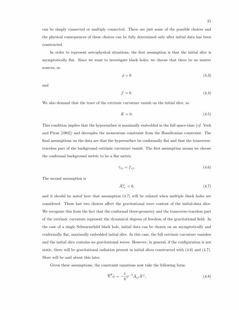
is actually that of two asymptotically flat spaces joined at the spherical surface r = r′ = κM/16π

(see Figure 4.1), and this implies that the manifold is complete.

r = r′ = κM/16π

1Figure 4.1: Embedding diagram of time-symmetric, maximal sliceof Schwarzschild geometry in isotropic coordinates.

These two asymptotically flat spaces are often referred to as the “top” and “bottom” sheets of

the manifold and the region connecting them is known as an Einstein-Rosen bridge (Einstein and

Rosen [1935]). The region interior to the event horizon on the top sheet, r < κM/16π, is not the

interior of the black hole, but is an identical “second” or “alternate” universe. This can be seen

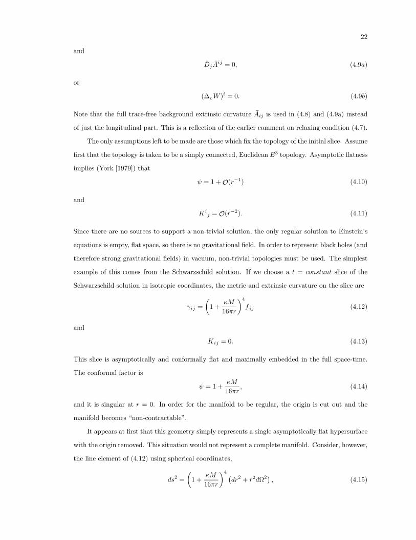
most easily by plotting the initial slice in the familiar Kruskal coordinates (Figure 4.2).

24

Singularity

Singularity

Black HoleInterior

Event Horizon

Σ“Other” Universe

Bottom Sheetr < κM/16π

“Our” UniverseTop Sheetr > κM/16π

1Figure 4.2: Time-symmetric, maximal slice of Kruskal space-time,labeled in isotropic coordinates and showing “top” and

“bottom” sheets in the two different universes.

This example illustrates the main principle followed in constructing vacuum, black-hole initial-

data sets: we use multiple asymptotically flat sheets connected by Einstein-Rosen bridges. In doing

this, two criteria must be satisfied in the resulting initial-data sets. The first is regularity and the

second is completeness of the manifold (cf. Brill and Lindquist [1963]).

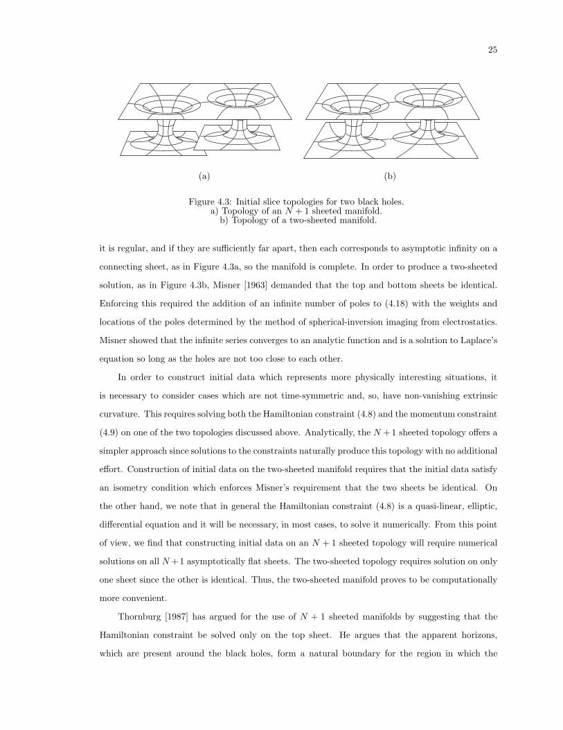
If we want to represent more than one black hole on the initial slice, then there are essentially

two avenues which can be taken in choosing the topology of the initial slice. Let us assume that

there are to be N black holes in our “universe”. One approach for modeling this is to allow each

of the holes to connect to its own isolated, asymptotically flat universe through an Einstein-Rosen

bridge. This produces an N + 1 sheeted manifold (Figure 4.3a). The second approach is to allow all

N holes to connect to the same alternate, asymptotically flat universe through N Einstein-Rosen

bridges. This produces a multiply-connected, two-sheeted manifold (Figure 4.3b).

Analytic solutions to the initial-value equations on both topologies have been found which

represent multiple black holes at a moment of time symmetry (Misner [1963], Lindquist [1963], and

Brill and Lindquist [1963]). If all of the holes are momentarily at rest, then the extrinsic curvature

vanishes everywhere on the initial slice and the Hamiltonian constraint (4.8) reduces to Laplace’s

equation. A solution representing N black holes is

ψ = 1 +N∑α=1

µα|x−Cα|

, (4.18)

where µα are constants related to the masses of the holes and the points Cα are the positions of the

centers of the holes in the background space. The points Cα are deleted from the manifold so that

25

(a) (b)

1Figure 4.3: Initial slice topologies for two black holes.a) Topology of an N + 1 sheeted manifold.

b) Topology of a two-sheeted manifold.

it is regular, and if they are sufficiently far apart, then each corresponds to asymptotic infinity on a

connecting sheet, as in Figure 4.3a, so the manifold is complete. In order to produce a two-sheeted

solution, as in Figure 4.3b, Misner [1963] demanded that the top and bottom sheets be identical.

Enforcing this required the addition of an infinite number of poles to (4.18) with the weights and

locations of the poles determined by the method of spherical-inversion imaging from electrostatics.

Misner showed that the infinite series converges to an analytic function and is a solution to Laplace’s

equation so long as the holes are not too close to each other.

In order to construct initial data which represents more physically interesting situations, it

is necessary to consider cases which are not time-symmetric and, so, have non-vanishing extrinsic

curvature. This requires solving both the Hamiltonian constraint (4.8) and the momentum constraint

(4.9) on one of the two topologies discussed above. Analytically, the N + 1 sheeted topology offers a

simpler approach since solutions to the constraints naturally produce this topology with no additional

effort. Construction of initial data on the two-sheeted manifold requires that the initial data satisfy

an isometry condition which enforces Misner’s requirement that the two sheets be identical. On

the other hand, we note that in general the Hamiltonian constraint (4.8) is a quasi-linear, elliptic,

differential equation and it will be necessary, in most cases, to solve it numerically. From this point

of view, we find that constructing initial data on an N + 1 sheeted topology will require numerical

solutions on all N+1 asymptotically flat sheets. The two-sheeted topology requires solution on only

one sheet since the other is identical. Thus, the two-sheeted manifold proves to be computationally

more convenient.

Thornburg [1987] has argued for the use of N + 1 sheeted manifolds by suggesting that the

Hamiltonian constraint be solved only on the top sheet. He argues that the apparent horizons,

which are present around the black holes, form a natural boundary for the region in which the

26

Hamiltonian constraint must be solved. Doing this, however, ignores the remainder of the initial-

data slice. While information can never cross the apparent horizons into the top sheet during the

time evolution, this does not preclude the existence of global structures which can be located only

by knowing the initial data on the complete manifold as I will show later (cf. Cook and York [1990]).

The final assumption of the conformal imaging approach is to assume that the initial-data

manifold has a two-sheeted topology and that the sheets are related by an isometry which requires

the two sheets, and any fields on them, to be identical. The approach, for the case of a single hole,

was detailed by Bowen [1979b] and Bowen and York [1980]. The extension for multiple holes was

carried out by Kulkarni, Shepley, and York [1983]. In the remainder of this chapter, I will outline

the approach, closely following Kulkarni et al. [1983].

LetMN denote the two-sheeted manifold containingN Einstein-Rosen bridges, each representing

a single black hole. To construct the manifold, take two identical, three-dimensional Euclidean spaces

E3 with N non-intersecting spheres, located at Cα and with radii aα (α = 1, . . . , N), removed. The

two spaces will represent the top and bottom sheets of MN and will be labeled, respectively, by Y

and Z. If p = (p1, p2, p3) represents a point in either sheet, then the sheets are defined by

Y = Z ≡

p ∈ E3 : |p−Cα| > aα, α = 1, . . . , N. (4.19)

The collection of boundaries B is defined as

B ≡N⋃α=1

Bα where Bα ≡

p ∈ E3 : |p−Cα| = aα. (4.20)

Let the union of the top sheet and the boundary be Y ≡ Y ∪ B, and similarly Z ≡ Z ∪ B. The

manifold MN is now defined as MN ≡ Y ∪ Z, with the boundaries Bα (each representing a throat

or bridge) identified. To put coordinates on the manifold, we define a collection of coordinate maps

Ψα on MN , each covering Y and Z through the αth throat. Let x denote the range of points in E3

covered by the maps and define

X ≡

x ∈ E3 : |x−Cα| > aα, α = 1, . . . , N

(4.21)

and

Sα ≡

x ∈ E3 : |x−Cα| = aα. (4.22)

We can now define the maps Jα which identify the two sheets through each of the throats

Jα : E3 − aα → E3 − aα (4.23)

27

by

Jα (x) ≡(a2α

rα

)nα + Cα, (4.24)

where

rα = |x−Cα| (4.25)

and

nα =(x−Cα)

rα. (4.26)

We now define the αth image of X as

Iα = Jα [X] , (4.27)

and the αth coordinate map as

Ψα : (Y ∪Bα ∪ Z)→ (X ∪ Sα ∪ Iα) , (4.28)

where

Ψα(p) =

(p1, p2, p3) ∈ (X ∪ Sα), if p ∈ (Y ∪Bα)Jα(p1, p2, p3) ∈ Iα, if p ∈ Z.

(4.29)

Note that J2α is the identity operator since

Jα [Jα [X]] = X, (4.30)

and so Jα is its own inverse.

For the case of one hole, we recover exactly the manifold structure seen previously for the

Schwarzschild black hole. In this case, one coordinate patch will smoothly cover the entire manifold.

If we consider the two sheets separately, we have points on the top sheet labeled by (r, θ, φ), and

on the bottom sheet by (r′, θ′, φ′). From (4.29), points on the top sheet will have coordinates

(r, θ, φ), while a point on the bottom sheet will have coordinates J1(r′, θ′, φ′). In terms of spherical

coordinates this yields (r =

a21

r′, θ = θ′, φ = φ′

), (4.31)

which is just the coordinate transformation (4.16) with a1 = κM/16π. So spherical coordinates with

the origin removed correspond, in this case, to the single coordinate patch for a single Einstein-Rosen

bridge topology, with the region interior to r = κM/16π being the bottom sheet.

In addition to having a two-sheeted manifold, it is required that any fields on the two sheets of

the manifold must be identical. More precisely, we require that the isometry between the sheets be

generated by the maps Jα via the pull-back maps J∗α. That is,

(data at x ∈ X) = ±J∗α (data at Jα (x)) . (4.32)

28

The change of sign is allowed since the square of a map is the identity (4.30) and since it will

give physically meaningful results. Since the second sheet is covered in its entirety by N different

coordinate maps Iα (4.27), it is required for consistency that (4.32) be satisfied not for a single α

but for all α = 1, . . . , N . This guarantees that fields on the bottom sheet will be identical to the

fields on the top sheet no matter which coordinate map is used.

In the case of a scalar field Φ on the manifold, the isometry condition (4.32) requires

Φ (x) = ±Φ (Jα (x)) . (4.33)

For a one-form ωi, (4.32) requires

ωi (x) = ±(Jα)ijωj (Jα (x)) , (4.34)

where

(Jα)ij ≡ ∂(Jα)j

∂xi(4.35)

is the Jacobian of the map Jα. For a vector field V i, (4.32) requires

V i (x) = ±(J−1α

)jiV j (Jα (x)) , (4.36)

where the inverse Jacobian, defined by

(J−1α

)ki(Jα)j

k = δkj , (4.37)

is used. The extension to other tensor fields is obvious.

The two fields of importance for gravitational initial data are the metric and extrinsic curvature.

These must satisfy

γij (x) = ±(Jα)ik(Jα)j`γk` (Jα (x)) (4.38)

and

Aij (x) = ±(Jα)ik(Jα)j`Ak` (Jα (x)) . (4.39)

To explore the isometry conditions on the background fields, consider the form that the Jacobian

(4.35) and the inverse Jacobian take in Cartesian coordinates:

(Jα)ij =a2α

r2α

(δji − 2njαn

αi

)(4.40a)

and (J−1α

)ij =

r2α

a2α

(δji − 2njαn

αi

). (4.40b)

29

Using the conformal decomposition of the metric (3.1) and the assumption that the background

metric is flat (4.6), the isometry condition on the metric becomes

ψ4 (x) f ij = ±(Jα)ik(Jα)j`ψ4 (Jα (x)) fk`. (4.41)

Using the explicit form of the Jacobian (4.40), this reduces to

ψ4 (x) f ij = ±(aαrα

)4

ψ4 (Jα (x)) f ij , (4.42)

or more simply

ψ (x) =aαrαψ (Jα (x)) . (4.43)

Note that the isometry condition with a minus sign is not allowed since this would imply the

conformal factor vanishes on each throat which would make the metric singular. Now, if we consider

the conformal transformation of the extrinsic curvature, we find from (3.9) and (4.39)

ψ−2 (x) Aij (x) = ±(Jα)ik(Jα)j`ψ−2 (Jα (x)) Ak` (Jα (x))

= ±(Jα)ik(Jα)j`(aαrα

)2

ψ−2 (x) Ak` (Jα (x)), (4.44)

or using (4.40),

Aij (x) = ±(aαrα

)6 (δki − 2nkαn

αi

) (δ`j − 2n`αn

αj

)Ak` (Jα (x)) . (4.45)

Equations (4.43) and (4.45) are conditions which solutions to the two constraint equations (4.8)

and (4.9) must satisfy in order to represent inversion-symmetric initial data on a regular, complete,

two-sheeted initial slice. Since the background fields on the two sheets of the manifold are related by

(4.43) and (4.45), it is only necessary to solve the constraints on one sheet, provided these relations

are compatible with the constraints. Assume that ψ(x) and Aij(x ) are solutions of (4.8) and (4.9a)

in the region X defined by

X = XN⋃α=1

Sα, (4.46)

that is, the top sheet plus all of the throats. Now consider the coordinate patch Ψα and let ψ(x )

and Aij(x ) be defined for x in the region Iα. They will take values via the two relations (4.43) and

(4.45) for the αth hole:

ψ (x) =aαrαψ (Jα (x)) (4.47)

Aij (x) = ±(aαrα

)6 (δki − 2nkαn

αi

) (δ`j − 2n`αn

αj

)Ak` (Jα (x)) (4.48)

30

To simplify notation, let x′ ≡ Jα(x). From (4.30), this gives

x = Jα(x′). (4.49)

Using the following definitions,

r′α ≡ |x′ −Cα| and n′α ≡(x′ −Cα)

r′α, (4.50)

one finds:

rα = rα (Jα (x′)) =a2α

r′α(4.51)

and

nα = nα (Jα (x′)) = n′α. (4.52)

The data on the bottom sheet can now be written as

ψ (x) =r′αaαψ (x′) (4.53)

and

Aij (x) = ±(r′αaα

)6 (δki − 2n′kα n

′αi

) (δ`j − 2n′`αn

′αj

)Ak` (x′) . (4.54)

Checking to see if the extrinsic curvature on the bottom sheet satisfies the momentum constraint,

we find

DjAij (x) = ±(Jα)jmD′m

((r′αaα

)6 (fki − 2n′kα n

′iα

) (f `j − 2n′`αn

′jα

)Ak` (x′)

)

= ±(r′αaα

)8 (δik − 2n′αk n

′iα

)D′jA

kj (x′) ,

(4.55)

where D′m is the background covariant derivative with respect to x′. Thus, the extrinsic curvature

on the bottom sheet, as given by (4.48), satisfies the momentum constraint (4.9), if the top-sheet

extrinsic curvature defining it satisfies the momentum constraint.

To check the Hamiltonian constraint, we first examine the right-hand side of (4.8). From (4.54),

we findAij (x) Aij (x) = f ikf j`Aij (x) Ak` (x)

=(r′αaα

)12

Aij (x′) Aij (x′) ,(4.56)

and, together with (4.53), this gives

ψ−7 (x) Aij (x) Aij (x) =(r′αaα

)5

ψ−7 (x′) Aij (x′) Aij (x′) . (4.57)

31

Next, the Laplacian of the conformal factor gives

∇2ψ (x) = f ij(Jα)ikD′k

[(Jα)j`D′`

(r′αaα

)ψ (x′)

]=(r′αaα

)5

∇′2ψ (x′) .

(4.58)

Thus, the Hamiltonian constraint for the conformal factor on the bottom sheet,

∇2ψ (x) +

18ψ−7 (x)Aij (x) Aij (x)

=(r′αaα

)5(∇′

2ψ (x′) +

18ψ−7 (x′) Aij (x′) Aij (x′)

),

(4.59)

is satisfied if the top-sheet conformal factor defining it satisfies the Hamiltonian constraint and if

the extrinsic curvature is inversion-symmetric.

We can now summarize the conformal imaging method as an approach for computing initial data

which represents multiple black holes with non-vanishing initial linear and angular momenta in an

asypmtotically flat universe. First, demand that the initial-data slice consist of two asymptotically

flat universes connected via N Einstein-Rosen bridges, one for each black hole. Next, demand that

physical fields in the two universes be “identical”. We choose the initial-data slice to be conformally

flat and maximally embedded in the full space-time manifold.

Working in the flat conformal background space, we start by taking a full three-dimensional

Eulcidean three-manifold E3 as the domain in which we must determine the initial data. For

each black hole which will be present in our universe, we choose its “position” Cα and its “radius”

aα (α = 1, . . . , N). The N spheres of radius aα are removed from the manifold E3 and the remainder,

E3 − aα, is the domain in which we must determine the initial data.

In the domain E3−aα, we first find solutions to the momentum constraint (4.9) which satisfy

the isometry condition (4.45). By satisfying the isometry condition (4.45), the background extrinsic

curvature is said to be inversion symmetric. It is guaranteed to generate a solution on the second

sheet which satisfies the momentum constraint, and when combined with an inversion-symmetric

conformal factor, will yield a physical extrinsic curvature which is regular everywhere and satisfies

the condition (4.39) that it be “identical” on the two sheets.

Given an inversion-symmetric background extrinsic curvature, a solution must be found for the

Hamiltonian constraint (4.8) which satisfies the isometry condition (4.43). By satisfying the isometry

condition (4.43), the conformal factor is said to be inversion symmetric. It is guaranteed to generate

a solution on the second sheet which satisfies the Hamiltonian constraint and, when combined with

the flat Euclidean background metric, yields a physical metric which is regular everywhere and

represents a complete manifold consisting of two “identical”, asymptotically flat sheets.

Chapter 5: Solutions of the Momentum Constraint

Solving the momentum constraint equations is the first step in constructing inversion-symmetric

gravitational initial data. If the initial-data slice is chosen to be maximal, or more generally if the

trace of the extrinsic curvature is a constant on the initial slice, then the momentum constraint (4.2)

decouples from the Hamiltonian constraint (4.1). This is one of the prime strengths of the conformal

decomposition of the constraints, and can be exploited in certain cases to find analytic solutions for

the background extrinsic curvature. When the initial slice is conformally and asymptotically flat,

this decoupling also allows for the determination of two of the physical properties of the initial-data

slice without knowing the complete initial data, as is shown below.

The momentum contained in an asymptotically flat, initial-data slice can be calculated from

the integral

Πiξi(k) =

1κ

∮∞

(Ki

j − δjiK)ξi(k)d

2Sj , (5.1)

where ξi(k) is a Killing vector of the spatial metric γij (York [1980]). In the conformal imaging

approach, the initial slice is conformally flat, as well as asymptotically flat. Since the background

metric is flat and the conformal factor must behave like (4.10) at infinity, the integral (5.1) can be

expressed equivalently in terms of the background extrinsic curvature and the flat metric. Recalling

(4.5), we can now rewrite (5.1) as

Πiξi(k) =

1κ

∮∞Ai

j ξi(k)d2Sj . (5.2)

Here, the integral is in terms of the flat background metric, and ξi(k) is a Killing vector of the flat

background metric fij to which γij is asymptotic. If ξi(k) is a translational Killing vector, then

Πiξi(k) is the linear momentum Pk. In terms of Cartesian coordinates, the total physical linear

momentum of a slice is given by

P i =1κ

∮∞Aijd2Sj . (5.3)

If ξi(k) is a rotational Killing vector, then Πiξi(k) is the angular momentum Sk. In terms of Cartesian

coordinates, the total physical angular momentum of a slice is given by

Si =1κεijk

∮∞xjAk`d2S`. (5.4)

33

It should be noted that the angular momentum at infinity is not always well defined. The angular

momentum Sk will be asymptotically gauge invariant, however, if ξi(k) is an exact symmetry of

the the physical metric γij (cf. York [1980]). So, given a solution for the background extrinsic

curvature, we see from (5.3) and (5.4) that two important properties of the physical initial-data

set can be determined without knowing the full initial data, i.e., without solving the Hamiltonian

constraint.

In the context of the conformal imaging approach, we would like to find solutions to the mo-

mentum constraint (4.9) which satisfy the isometry condition (4.45) and represent black holes with

linear momentum P iα and angular momentum Siα as determined by (5.3) and (5.4). For the case of

a single black hole, Bowen and York [1980] have found such solutions and they take the following

form:A±ij =

3κ16πr2

[P inj + P jni − (f ij − ninj)P knk

]∓ 3κa2

16πr4

[P inj + P jni + (f ij − 5ninj)P knk

] (5.5)

and

Aij =3κ

8πr3

[εki`S

`nknj + εkj`S`nkni

]. (5.6)

Note, that we have dropped the subscript α on a, r, ni, P i, and Si since there is only one hole.

Equation (5.5) gives the background extrinsic curvature for a hole with linear momentum P i and

is actually two solutions. The solution A+ij satisfies the isometry condition (4.45) with the plus

sign, and the solution A−ij satisfies the isometry condition (4.45) with the minus sign. Only the

O(r−2) term in (5.5) carries linear momentum as can be seen by evaluating (5.3). The second term

is required for inversion symmetry. The two terms are individually solutions of the momentum

constraint (4.9a). Equation (5.6) gives the background extrinsic curvature for a hole with angular

momentum Si. This solution satisfies the isometry condition with the minus sign only and is its

own inverse.

The solutions (5.5) and (5.6) are longitudinal since they can be derived from a vector potential.

O Murchada and York [1976a] found solution to (4.9b) for the vector potential W i for the first term

in (5.5) and for (5.6). Bowen [1979a] found the solution giving the second term in (5.5). The first

term in (5.5), the part carrying linear momentum, is derived from the vector potential

W i = − κ

32πr[7P i + ninjP

j]. (5.7)

The second part of (5.5) can also be derived from a vector potential. It takes the form

W i =κa2

32πr3

[P i − 3ninjP j

]. (5.8)

34

As previously mentioned, this term carries no linear momentum and is present only to enforce

inversion symmetry. The solution representing a black hole with spin, (5.6), is derived from the

vector potential

W i =κ

8πr2εijknjSk. (5.9)

The solutions (5.5) and (5.6) satisfy all of the conditions required by the conformal imaging

approach and can be used with the Hamiltonian constraint to construct inversion-symmetric initial

data for a single hole with linear and angular momentum. Such initial data has been constructed

by many researchers (cf. York and Piran [1982], Choptuik and Unruh [1986], Rauber [1985], and

Cook and York [1990]) and will be examined in later chapters. I will proceed here with the question

of how to construct an inversion-symmetric solution of the momentum constraint for systems with

multiple black holes.

This problem was addressed formally by Kulkarni, Shepley, and York [1983]. The approach is

centered on the fact that the momentum constraint (4.9) is linear. Since this is the case, a solution

representing N black holes, each with linear and angular momentum can be obtained from (5.5) and

(5.6) as

Aij =3κ8π

N∑α=1

(1

2r2α

[Pαi n

αj + Pαj n

αi −

(fij − nαi nαj

)P kαn

αk

]+

1r3α

[εki`S

`αn

kαn

αj + εkj`S

`αn

kαn

αi

]).

(5.10)

Note that the second term in (5.5) has been omitted here. The N black holes are given individual

linear and angular momenta P iα and Siα in the sense that if the holes are “sufficiently far apart”,

then they will have such momenta as measured by (5.3) and (5.4). If the holes are close together,

then all that can be measured is the total linear and angular momentum of the system.

The background extrinsic curvature given by (5.10) is longitudinal and traceless and is a solution

of the momentum constraint (4.9), however, it is not inversion symmetric through any of the holes

as is required. This is why the second term in (5.5) was not included for each hole in (5.10).

Even though (5.10) is not inversion symmetric, Kulkarni et al. [1983] have shown how to take this

non-invertable extrinsic curvature and make it inversion symmetric through a method of images

applicable to tensors. I will outline the formal approach below.

In order for the extrinsic curvature to be inversion symmetric, it must satisfy

Aij (x) = <±α Aij (x)

= ±(aαrα

)2

(Jα)i`A`m (Jα (x)) (Jα)jm(5.11)

35

for all α. In order to simplify and clarify notation, I will drop the component indices and write

(5.11) asA (x) = <±α A (x)

= ±(aαrα

)2

(x)

[Jα](x)A (Jα (x)) [Jα](x).(5.12)

Note that in order to distinguish the Jacobian from the transformation Jα, the Jacobian is enclosed

in square brackets. Let Mij(x) be any second rank tensor field on E3. It is straightforward to show

the following properties of the inversion operator <±α (cf. Kulkarni et at [1983]).

<±α <±α = II . (5.13)

(<±α M

)t = <±α (M t), (5.14)

where M t is the transpose of M .

[Tr(<±α M

)](x)

= ±(aαrα

)6

(x)

[(TrM)(Jα(x))

], (5.15)

where TrM is the trace of M .

[Dj

(<±α M ij

)](x)

= ±(aαrα

)6

(x)

(Jα)(x)k

i[D`M

k`](Jα(x))

+ 2(niαrα

)(x)

[TrM ](Jα(x))

.

(5.16)

If we start with a symmetric and traceless solution, Aij , to the momentum constraint (4.9a),

then (5.14), (5.15), and (5.16) guarantee that the “image” of it, <±α Aij , will also be symmetric,

traceless, and satisfy the momentum constraint. Now consider the following operator:

<± = II +∑αi

(m∏i=1

<±αi

). (5.17)

The notation here needs some elaboration. The αi label the holes as usual and the subscript i takes

on the values of 1, . . . , N . The sum is over all unique sequences αi of length m. For any sequence,

αi, one takes the product of “image” operators corresponding to that sequence. From property

(5.13), a sequence is unique if and only if αi 6= αi+1. As an example of this operator, consider the

case of a single hole. The operator (5.17) takes, in this case, the form

<± = II + <±α1. (5.18)

For two holes, it takes the form

<± = II + <±α1+ <±α1

<±α2+ <±α1

<±α2<±α1

+ <±α1<±α2

<±α1<±α2

+ · · ·

+ <±α2+ <±α2

<±α1+ <±α2

<±α1<±α2

+ <±α2<±

α1<±α2

<±α1+ · · · .

(5.19)

36

It can be easily verified from (5.13), that

<±α <± = <± (5.20)

for all α and so (5.17) can be called the inversion symmetry operator. If it acts on any arbitrary

second rank tensor Mij , then the result will be inversion symmetric through all N holes. In par-

ticular, if Mij is symmetric, traceless, and satisfies the momentum constraint, then <±Mij will be

symmetric, traceless, satisfy the momentum constraint, and be inversion symmetric.

The formal approach for obtaining an inversion-symmetric solution of the momentum constraint

(4.9a) is now obvious. Let Aij represent a sum of single hole solutions to the momentum constraint.

The inversion-symmetric solution is then given by

Aij = <±Aij . (5.21)

In the case of a single hole, (5.21) will be Aij plus a single image term. Specifically, it will be a

combination of (5.5) and (5.6). If there is more than one hole, then (5.21) will consist of Aij plus

an infinite number of image terms. In this case, one must be concerned with the convergence of

this infinite series. Kulkarni [1984] has shown that for any reasonable choice for Aij , the infinite

series converges if the holes are far enough apart. In particular, if there are just two holes, then

the infinite series converges absolutely provided the inversion surfaces do not overlap. This is in

direct analogy with Misner’s proof of convergence for the inversion-symmetric conformal factor on

a time-symmetric initial slice (Misner [1963]).

To continue, we need to specify an explicit form for Aij . A first guess would be to use (5.10).

This would lead to an error in the computation of spins since the αth spin term in (5.10) is the

negative of its inverse through the αth hole. Using (5.10) in (5.21) would result in holes with twice

the desired spin for each hole. There is no problem with the terms containing linear momentum

since the full, inversion-symmetric form is not used. This error pertaining to the spin exists in

Kulkarni et al. [1983], Kulkarni [1984], and York [1984]. Bowen, Rauber, and York [1984] correct

for this error by redefining (5.21) with an overall factor of 1/2. This will work provided that the

full, inversion-symmetric solutions containing linear momentum (5.5) are used. One must be careful,

however, to choose the correct sign in (5.5) to match that of (5.21). The more elegant, and more

computationally convenient method, is to define Aij as

Aij =3κ16π

N∑α=1

(1r2α

[Pαi n

αj + Pαj n

αi −

(fij − nαi nαj

)P kαn

αk

]+

1r3α

[εki`S

`αn

kαn

αj + εkj`S

`αn

kαn

αi

]).

(5.22)

37

Consider now, the total linear and angular momenta contained in the inversion-symmetric

background extrinsic curvature defined by (5.17), (5.21), and (5.22). Aij will contain three types of

terms. First, it will contain Aij itself. It will also contain the self-image of each term in Aij . Finally,

it will contain arbitrary image terms. Computing the total linear momentum (5.3) from Aij yields

the sum of the individual linear momenta Pαi . As has already been mentioned, the self-image of the

linear momentum terms carry no linear or angular momentum.

If we next assume that none of the holes has any linear momentum, then the total angular

momentum (5.4) contained in Aij is simply half the sum of the individual angular momenta Sαi . If

we choose the isometry relation with the minus sign, then the self-image of the angular momentum

terms again carries half the sum of the individual angular momenta Sαi . This is why (5.22) is used

instead of (5.10). If the isometry relation with the plus sign is used, the angular momentum from

the self-image terms will cancel that from Aij . If the holes have non-zero linear momentum, then the

linear momentum terms in Aij can contain non-zero angular momentum although their self-image

terms cannot.

Remaining to be examined are the contributions to the total linear and angular momentum

from the general image terms. Bowen, Rauber, and York [1984] detail an elegant proof that no

general image term can carry angular momentum. Their proof, however, cannot be generalized to

examine their linear momentum content. Through tedious, explicit calculations, it can be shown

that at large distances from the holes, the leading behavior of all of the general image terms is

O(r−6). A term with this fall-off behavior contributes nothing to the integrals (5.3) and (5.4) and

thus carries no linear or angular momentum. This is a very powerful result. It means that the total

linear and angular momentum content of an initial-data slice can be computed without knowing the

explicit form of the general image terms. The only terms which contribute are the “base” extrinsic

curvature Aij and the self-image terms of the angular momentum terms (which are trivial).

As a final note to the formalism for constructing inversion-symmetric extrinsic curvature solu-

tions, it should be pointed out that the imaging is done on the purely longitudinal field Aij and not

the potential W i. For the case of a single black hole, the resulting, imaged field Aij is still longi-

tudinal. In the case of multiple black holes, this does not seem to be the case. Rauber [1985] has

shown in a lengthy calculation that the resulting field Aij is not derivable from a vector potential.

This implies that Aij contains some transverse components. This is not a problem since we are free

to specify the transverse-tracefree content of the extrinsic curvature. This is the reason that the less

restrictive form of the momentum constraint (4.9a) has been retained and explains further the note

that the assumption (4.7) would be relaxed.

38

At this point, we have a formalism for the construction of inversion-symmetric, background

extrinsic curvatures. In order to find solutions to the Hamiltonian constraint, we must be able to

move past the formalism and find a concrete method for computing these extrinsic curvatures. In

the case of a single hole, the resulting inversion-symmetric, background extrinsic curvature is given

in (5.5) and (5.6). If we consider more than one hole, the evaluation of an infinite series must be

dealt with.

The situation of primary concern is the two body problem so we need to find a method for

calculating the extrinsic curvature for two holes. Bowen, Rauber, and York [1984] have addressed this

problem for a certain special case. They considered the situation in which the two holes are of equal

size, have no linear momentum, and have angular momenta which are equal in magnitude. With

the further restriction that the direction of the angular momenta be either aligned or anti-aligned

with the axis between the two holes, they found an analytic expression for each term in the infinite

series. Even in this situation, which contains a high degree of symmetry, their method is tedious

and results in an expression involving complicated combinations of hyperbolic and trigonometric

functions. If this approach is applied to the case of axially aligned linear momentum or to the case

where the linear or angular momentum is not axisymmetric, then the method becomes completely

intractable. In order to proceed, another avenue must be taken. The solution which I have found to

the problem is to abandon the attempt to find an analytic expression for each term in the infinite

series. Instead, the solution lies in a constructive, computational approach which I detail in the next

chapter.

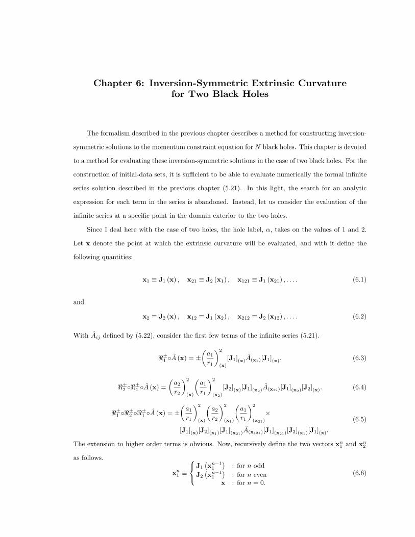
Chapter 6: Inversion-Symmetric Extrinsic Curvaturefor Two Black Holes

The formalism described in the previous chapter describes a method for constructing inversion-

symmetric solutions to the momentum constraint equation for N black holes. This chapter is devoted

to a method for evaluating these inversion-symmetric solutions in the case of two black holes. For the

construction of initial-data sets, it is sufficient to be able to evaluate numerically the formal infinite

series solution described in the previous chapter (5.21). In this light, the search for an analytic

expression for each term in the series is abandoned. Instead, let us consider the evaluation of the

infinite series at a specific point in the domain exterior to the two holes.

Since I deal here with the case of two holes, the hole label, α, takes on the values of 1 and 2.

Let x denote the point at which the extrinsic curvature will be evaluated, and with it define the

following quantities:

x1 ≡ J1 (x) , x21 ≡ J2 (x1) , x121 ≡ J1 (x21) , . . . . (6.1)

and

x2 ≡ J2 (x) , x12 ≡ J1 (x2) , x212 ≡ J2 (x12) , . . . . (6.2)

With Aij defined by (5.22), consider the first few terms of the infinite series (5.21).

<±1 A (x) = ±(a1

r1

)2

(x)

[J1](x)A(x1)[J1](x). (6.3)

<±2 <±1 A (x) =

(a2

r2

)2

(x)

(a1

r1

)2

(x2)

[J2](x)[J1](x2)A(x12)[J1](x2)[J2](x). (6.4)

<±1 <±2 <

±1 A (x) = ±

(a1

r1

)2

(x)

(a2

r2

)2

(x1)

(a1

r1

)2

(x21)

×

[J1](x)[J2](x1)[J1](x21)A(x121)[J1](x21)[J2](x1)[J1](x).

(6.5)

The extension to higher order terms is obvious. Now, recursively define the two vectors xn1 and xn2

as follows.

xn1 ≡

J1

(xn−1

1

): for n odd

J2

(xn−1

1

): for n even

x : for n = 0.(6.6)

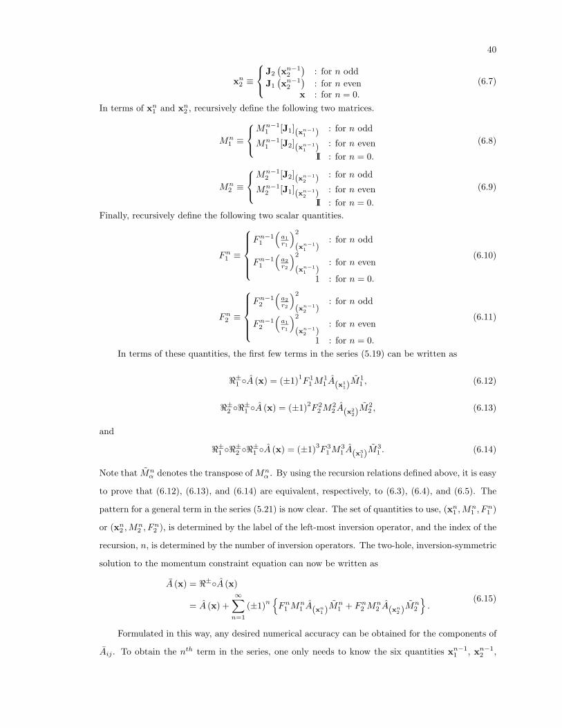
40

xn2 ≡

J2

(xn−1

2

): for n odd

J1

(xn−1

2

): for n even

x : for n = 0.(6.7)

In terms of xn1 and xn2 , recursively define the following two matrices.

Mn1 ≡

Mn−1

1 [J1](xn−11 ) : for n odd

Mn−11 [J2](xn−1

1 ) : for n evenII : for n = 0.

(6.8)

Mn2 ≡

Mn−1

2 [J2](xn−12 ) : for n odd

Mn−12 [J1](xn−1

2 ) : for n evenII : for n = 0.

(6.9)

Finally, recursively define the following two scalar quantities.

Fn1 ≡

Fn−1

1

(a1r1

)2

(xn−11 )

: for n odd

Fn−11

(a2r2

)2

(xn−11 )

: for n even

1 : for n = 0.

(6.10)

Fn2 ≡

Fn−1

2

(a2r2

)2

(xn−12 )

: for n odd

Fn−12

(a1r1

)2

(xn−12 )

: for n even

1 : for n = 0.

(6.11)

In terms of these quantities, the first few terms in the series (5.19) can be written as

<±1 A (x) = (±1)1F 1

1M11 A(x1

1)M11 , (6.12)

<±2 <±1 A (x) = (±1)2

F 22M

22 A(x2

2)M22 , (6.13)

and

<±1 <±2 <

±1 A (x) = (±1)3

F 31M

31 A(x3

1)M31 . (6.14)

Note that Mnα denotes the transpose of Mn

α . By using the recursion relations defined above, it is easy

to prove that (6.12), (6.13), and (6.14) are equivalent, respectively, to (6.3), (6.4), and (6.5). The

pattern for a general term in the series (5.21) is now clear. The set of quantities to use, (xn1 ,Mn1 , F

n1 )

or (xn2 ,Mn2 , F

n2 ), is determined by the label of the left-most inversion operator, and the index of the

recursion, n, is determined by the number of inversion operators. The two-hole, inversion-symmetric

solution to the momentum constraint equation can now be written as

A (x) = <±A (x)

= A (x) +∞∑n=1

(±1)nFn1 M

n1 A(xn1 )M

n1 + Fn2 M

n2 A(xn2 )M

n2

.

(6.15)

Formulated in this way, any desired numerical accuracy can be obtained for the components of

Aij . To obtain the nth term in the series, one only needs to know the six quantities xn−11 , xn−1

2 ,

41

Mn−11 , Mn−1

2 , Fn−11 , and Fn−1

2 which have already been computed in order to obtain the (n− 1)th

term. From a computational point of view, it is a simple iterative matter to keep adding terms until

the value of Aij converges to machine accuracy.

This formulation of the extrinsic curvature is completely general. It can be used to compute the

components of the extrinsic curvature when the two holes have any relative sizes and separation, and

for any values of the linear and angular momentum for each hole. In later chapters, I will explore

solutions to the Hamiltonian constraint in the case of axisymmetry. In preparation for this, I will

describe (6.15) explicitly for this special case.

Let us consider first the coordinate system to be used. Since the configuration is to be ax-

isymmetric, the obvious choice is to use cylindrical coordinates. It is best to use dimensionless

coordinates, so it is desirable to scale the coordinates relative to some physical length scale of the

problem. There are three natural length scales in the problem: the size of each of the two holes and

the separation between the two holes. I choose to use the radius of the first hole, a1, as the natural

length scale.

The two holes will be centered on the z-axis and will be positioned so that

C1 = [ 0 0 a1ζ1 ] and C2 = [ 0 0 a1ζ2 ] . (6.16)

In order to maintain axisymmetry, we choose the linear and angular momentum vectors for the

two holes to have components only in the z direction. The physical, unscaled linear and angular

momentum vectors will be

P1 = [ 0 0 P1 ] and P2 = [ 0 0 P2 ] (6.17)

and

S1 = [ 0 0 S1 ] and S2 = [ 0 0 S2 ] . (6.18)

The cylindrical coordinate components of Aij can now be written in dimensionless form as

Aρρa1

= − 3κ16π

(P1a1

)(z − ζ1)3(

ρ2 + (z − ζ1)2)5/2

+

(P2a1

)(z − ζ2)3(

ρ2 + (z − ζ2)2)5/2

, (6.19)

Aφφa1

= − 3κ16π

ρ2

(P1a1

)(z − ζ1)(

ρ2 + (z − ζ1)2)3/2

+

(P2a1

)(z − ζ2)(

ρ2 + (z − ζ2)2)3/2

, (6.20)

42

Azza1

=3κ16π

(P1a1

)(z − ζ1)

(ρ2 + 2(z − ζ1)2

)(ρ2 + (z − ζ1)2

)5/2

+

(P2a1

)(z − ζ2)

(ρ2 + 2(z − ζ2)2

)(ρ2 + (z − ζ2)2

)5/2

,

(6.21)

Aρza1

=3κ16π

ρ

(P1a1

)(ρ2 + 2(z − ζ1)2

)(ρ2 + (z − ζ1)2

)5/2+

(P2a1

)(ρ2 + 2(z − ζ2)2

)(ρ2 + (z − ζ2)2

)5/2

, (6.22)

Aρφa1

=3κ16π

ρ3

(S1a2

1

)(ρ2 + (z − ζ1)2

)5/2+

(S2a2

1

)(ρ2 + (z − ζ2)2

)5/2

, (6.23)

and

Aφza1

=3κ16π

ρ2

(S1a2

1

)(z − ζ1)(

ρ2 + (z − ζ1)2)5/2

+

(S2a2

1

)(z − ζ2)(

ρ2 + (z − ζ2)2)5/2

. (6.24)

Before describing the explicit form which the isometry map and the Jacobian will take, it is

useful to examine the square of the background extrinsic curvature which is the quantity of interest

in the Hamiltonian constraint. Expressed as a dimensionless quantity, it takes the form

a21AijA

ij =

(<±( A

a1

))ρρ

2

+

1ρ2

(<±

(A

a1

))φφ

2

+

[(<±

(A

a1

))zz

]2

+ 2

(<±( A

a1

))ρz

2

+ 2

1ρ

(<±

(A

a1

))ρφ

2

+ 2

1ρ

(<±

(A

a1

))φz

2

.

(6.25)

It is clear that care will have to be taken in computing the second, fifth, and sixth terms in (6.25) so

as not to encounter errors resulting from division by zero (not to mention computational roundoff

errors) as the ρ = 0 axis is approached. The second term in (6.25) is handled easily by the property

that Aij is traceless. This fact immediately gives

1ρ2

(<±

(A

a1

))φφ

= −

(<±( A

a1

))ρρ

+

[(<±

(A

a1

))zz

] , (6.26)

so we never actually need to compute this term. The fifth and sixth terms of (6.25) cannot be

handled so easily. Their resolution depends on the explicit form of the isometry and the Jacobian

in the scaled cylindrical coordinate system.

In order to define the isometry conditions, one more definition must be made. The scaled centers

of the holes have already been defined by (6.16). The scaled radius of the first hole is just one since

43

that length sets the scale for all quantities. All that remains is to define a dimensionless quantity to

give the size of the second hole. I define this quantity by the following:

a1 = αa2. (6.27)

A straightforward calculation shows that the isometry conditions take the following dimension-

less forms:

J1 (x) =[ ρρ2+(z−ζ1)2 , φ , z−ζ1

ρ2+(z−ζ1)2 + ζ1]

(6.28)

and

J2 (x) =[

α−2ρρ2+(z−ζ2)2 , φ , α

−2(z−ζ2)

ρ2+(z−ζ2)2 + ζ2

]. (6.29)

Based on these two equations, the Jacobians are given by

[J1](x) =

(z−ζ1)2−ρ2

(ρ2+(z−ζ1)2)2 0 −2ρ(z−ζ1)

(ρ2+(z−ζ1)2)2

0 1 0−2ρ(z−ζ1)

(ρ2+(z−ζ1)2)2 0 ρ2−(z−ζ1)2

(ρ2+(z−ζ1)2)2

(6.30)

and

[J2](x) =

α−2((z−ζ2)2−ρ2)(ρ2+(z−ζ2)2)2 0 −2α−2ρ(z−ζ2)

(ρ2+(z−ζ2)2)2

0 1 0−2α−2ρ(z−ζ2)

(ρ2+(z−ζ2)2)2 0α−2(ρ2−(z−ζ2)2)(ρ2+(z−ζ2)2)2

(6.31)

For completeness, I display the dimensionless form for the recursion relations (6.10) and (6.11):

Fn1 =

Fn−1

1ρ2+(z−ζ1)2

∣∣∣(xn−1

1 ): for n odd

α−2Fn−11

ρ2+(z−ζ2)2

∣∣∣(xn−1

1 ): for n even

1 : for n = 0

(6.32)

and

Fn2 =

α−2Fn−1

2ρ2+(z−ζ2)2

∣∣∣(xn−1

2 ): for n odd

Fn−12

ρ2+(z−ζ1)2

∣∣∣(xn−1

2 ): for n even

1 : for n = 0.

(6.33)

Consider now, in light of the explicit form of the recurrence relations, the form of the nth term

in the series (6.15). Explicit calculation shows that the ρρ, ρz, and zz terms depend only on Aρρ,

Aρz, and Azz. The ρφ and φz terms depend only on Aρφ and Aφz. Finally, the φφ term depends

only on Aφφ. This means that the linear and angular momentum pieces of the inversion-symmetric

extrinsic curvature are completely uncoupled and can be considered separately.

The two terms of concern in (6.25),

1ρ

(<±

(A

a1

))ρφ

and1ρ

(<±

(A

a1

))φz

, (6.34)

44

are angular momentum terms and, as mentioned above, depend only on Aρφ and Aφz. Looking

at (6.23) and (6.24), we see that both terms contain overall factors of ρ. This indicates that the

factors of 1/ρ should be “commuted” with the inversion operator. Consider the nth term of the first

expression in (6.34).1ρFn1

[Mn

1 A(xn1 )Mn1

]ρφ

+1ρFn2

[Mn

2 A(xn2 )Mn2

]ρφ. (6.35)

If we denote the ρ component of xnα as ρnα, then it is straightforward to verify that

1ρ

=Fnαρnα

. (6.36)

Equation (6.35) now becomes

(Fn1 )2

Mn1

[A

ρ

](xn1 )

Mn1

ρφ

+ (Fn2 )2

Mn2

[A

ρ

](xn2 )

Mn2

ρφ

, (6.37)

which is completely regular as the ρ = 0 axis is approached since it depends only on Aρφ and Aφz,

which both have overall factors of ρ. The second expression in (6.34) can be handled in exactly the

same manner.

The components of the background extrinsic curvature can now be accurately calculated in

cylindrical coordinates, with special care being given to the angular momentum terms. If axisym-

metry is not present, then a similar construction can be obtained in terms of Cartesian coordinates.

In this case, the linear and angular momentum components will not decouple, but there will be no

coordinate singularities to deal with.

Chapter 7: The Hamiltonian Constraint andBoundary Conditions

The final step in the construction of initial-data sets via the conformal imaging approach is the

solution of the Hamiltonian constraint (4.8). As shown in Chapter 4, the domain in which a solution

of the Hamiltonian constraint must be found is E3 − aα. That is, a three-dimensional Euclidean

flat space with N spheres cut out, one for each black hole. If proper boundary conditions can be

posed on the surfaces of these deleted spheres and at infinity, then the Hamiltonian constraint can

be posed as a quasi-linear, elliptic boundary value problem. Bowen and York [1980] have derived

such boundary conditions and these will be described below. I will also discuss some known, exact

solutions to the Hamiltonian constraint and the approach taken for finding numerical solutions.

In order to pose the Hamiltonian constraint as a boundary value problem, boundary conditions

must be found for all surfaces. The boundary condition at infinity has been discussed in Chapter 4.

It is fixed by the assumption that the initial-data slice is asymptotically flat. This, together with

the choice of a flat background metric, demands that the conformal factor behave like (4.10). Thus,

the first boundary condition is that the conformal factor is one at infinity. Along with the demand

that the metric be regular, this implies that the conformal factor always be greater than zero. In

practice, infinity is often not part of the domain of solution for the conformal factor when numerical

solutions are found. In this case, an approximate boundary condition must be used at large distances

from the holes. York and Piran [1982] have suggested and used an approximate boundary condition

which has become widely accepted. I will discuss it later in this chapter along with an improvement

which I have derived.

In order for the solution of the Hamiltonian constraint to be inversion symmetric, it must satisfy

the isometry condition (4.43) for every hole in the system. Consider the αth coordinate patch and

take a derivative of the isometry condition. The result is

Diψ (x) = −aαr2α

nαi ψ (Jα (x)) +aαrα

(Jα)ij[Djψ (x)

]Jα(x)

. (7.1)

If this is contracted with the αth unit normal and evaluated on the αth inversion boundary, the

result is

niαDiψ∣∣aα

= − ψ

2rα

∣∣∣∣aα

, (7.2)

46

where the fact that rα = aα is a fixed point set of the isometry has been used. That is, Jα(aα) = aα.

(7.2) represents a boundary condition which can be used on the surface of each deleted sphere. This

reduces directly to the boundary condition derived by Bowen and York [1980] in the case of a single

hole and to the form shown by Kulkarni et al. [1983] for the case of multiple holes.

Bowen and York [1980] have shown, in the case of a single hole, that the area of the inversion

boundary, or “throat”, is extremal. This result holds for the case of multiple holes as well and can

be seen as follows. Consider the area of a sphere of radius rα centered around the αth throat.

Aα =∮ψ4r2

αd2Ωα (7.3)

The condition for extremal area is found by varying the area and setting the variation to zero.

δAα = 2∮rαψ

3(2rαDiψ + ψnαi

)δxid2Ωα = 0 (7.4)

Considering only changes normal to the surface, (7.4) gives

niαDiψ +ψ

2rα= 0, (7.5)

which, together with (7.2), shows that the throats must be extremal surfaces.

The Hamiltonian constraint, together with the boundary conditions of asymptotic flatness at

infinity and inversion symmetry on the throats, constitutes a quasi-linear, elliptic boundary value

problem. In order for this boundary value problem to be well posed, it is necessary to show that any

solution satisfying the boundary conditions is unique. Two difficulties arise in trying to prove this.

One arises from the non-linearity of the Hamiltonian constraint and the other from the inversion

symmetry boundary condition (7.2). In order to deal with the non-linearity, one can consider a local

uniqueness proof. That is, it is shown that no other solutions lie in the neighborhood of a given

solution. This does not preclude the existence of other solutions which are “significantly different”.

If a standard, local uniqueness proof is attempted, it is found that the relative sign in (7.2) prevents

any conclusion. This is because (7.2) is an “anti-Robin” boundary condition, although it appears at

first sight to be a standard Robin condition (cf. Bergman and Schiffer [1953]). The problem arises

because niα points inward, into the domain of the solution, not outward.

In spite of these problems, York [1989] has proven that the solution for a single hole is locally

unique. This proof depends explicitly on the inversion symmetry of both the conformal factor and

the background extrinsic curvature. My attempts to generalize this proof to the case of multiple

holes have been unsuccessful. The presence of extra holes makes the method inconclusive. I believe

47

that the solution may depend on limits on the maximum hole-radius to hole-separation ratio as do

the convergence proofs of Misner [1963] and Kulkarni [1984] for the case of the infinite series which

arise when multiple holes are present.

In spite of the lack of any uniqueness proof in the case of multiple holes, I will continue on the

belief any solutions found will be locally unique and search for solutions. I will begin by looking at

the asymptotic behavior of the solutions to the Hamiltonian constraint. In doing this, I will follow

Bowen, Rauber, and York [1984] and use a “Newtonian” potential Φ instead of the conformal factor,

where Φ is defined by

ψ = 1− 12

Φ. (7.6)

The Hamiltonian constraint is very much like a Poisson equation except that the source term is

coupled non-linearly to the conformal factor. In terms of Φ, the Hamiltonian constraint is written

∇2Φ =

14ψ−7AijA

ij ≡ κ

2ρeff , (7.7)

where ρeff is defined as an effective energy density source. If we assume for a moment that ρeff has

compact support, then a multipole expansion of Φ is well defined outside the support and is given

by

Φ = − κ

8π

[E

r+din

i

r2+

32Iij(ninj − 1

3fij)

r3+O

(r−4)]. (7.8)

The monopole coefficient E is the total ADM energy contained in the initial-data slice (cf.

Arnowitt et al. [1962]). The other multipole coefficients are associated with the energy distribution

on the initial slice. These multipole coefficients are defined in terms of the following standard

Cartesian surface integrals:

E =2κ

∮∞DiΦd2Si, (7.9)

di =2κ

∮∞

(xiD

jΦ− δjiΦ)d2Sj , (7.10)

and

Iij =2κ

∮∞

[(xixj −

13r2f ij

)DkΦ−

(xiδ

kj + xjδ

ki −

23xkf ij

)Φ]d2Sk. (7.11)

The effective source does not, of course, have compact support. Because of this, the multipole

expansion will only be well defined through some given order defined by the radial fall off rate of the

source. From the conditions for asymptotic flatness (4.10) and (4.11), it is seen that the effective

source behaves as

ρeff = O(r−4). (7.12)

48

This means that the monopole term, and thus the total energy, is always well defined on an asymp-

totically flat slice.

The well behaved nature of the multipole expansion through monopole order is the basis of an

approximate boundary condition proposed by York and Piran [1982]. The conformal factor takes

the form

ψ = 1 +κ

16πE

r+O

(r−2). (7.13)

Taking the radial derivative of (7.13) and eliminating the total energy term results in the following

Robin boundary condition:∂ψ

∂r=

1− ψr

+1rO(r−2). (7.14)

Applied at large distances from the holes, (7.14) provides a good approximate outer boundary

condition. Exactly how far away the outer boundary must be for (7.14) to be a good approximation

depends on the explicit form of the effective source.

Evans [1989] has suggested that an improvement in the order of accuracy of the outer boundary

condition would be of great use in numerical solutions as it would allow the outer boundary to be

placed closer to the holes and reduce the size of the numerical problem. Prompted by this, I have

explored the possibility of incorporating higher order terms into the approximation. In general, (7.8)

is a valid expansion for Φ only through the monopole term. In order to make it valid for higher

order terms, it must be modified. Consider a function Λ which is not annihilated by the Laplacian

and which satisfies the following:

∇2Λ = O

(r−4)

= 4πρeff +O(r−5). (7.15)

Λ is thus chosen to compensate for the highest order effects of the effective source. I demand that

it have the following properties, in addition to (7.15):

Λ = O(r−2)

(7.16)

and

DiΛ = O(r−3). (7.17)

Now consider expanding Φ as

Φ = − κ

8π

[E

r+din

i

r2− Λ +O

(r−3)]. (7.18)

49

The total energy given by the monopole coefficient is still defined by (7.9) because of the fall-off

condition (7.17). The dipole term is modified and, in terms of (7.10), is given by

di = di −2κ

∮∞

(xiD

jΛ− δjiΛ)d2Sj . (7.19)

Given the fall-off conditions (7.16) and (7.17), the correction to the dipole moment will not, in

general, vanish and, thus, the “dipole moment” of (7.18) no longer represents a multipole moment

of the initial energy distribution. If the integral over Λ in (7.19) were to vanish either by some

symmetry or because (7.16) and (7.17) fall off faster than necessary, then the dipole moment would

retain its original interpretation and the multipole expansion would be well defined through dipole

order.

To proceed, we must have an explicit form for the function Λ. In order to determine this,

we must explore the asymptotic form of the effective source. Since the potential Φ is always well

defined through monopole order for asymptotically flat initial data, the asymptotic form of the

effective source is given by

ρeff =1

2κAijA

ij +O(r−5). (7.20)

Thus, in order to fix Λ, we need only consider the behavior of the background extrinsic curvature.

The asymptotic behavior of the extrinsic curvature is

Aij =3κ

16πr2

N∑α=1

[Pαi nj + Pαj ni − (f ij − ninj)P kαnk

]+O

(r−3). (7.21)

Using (7.21) in (7.20), the effective energy density is

4πρeff =9κ

64πr4

N∑α=1

N∑β=1

Pαi P

iβ + 2Pαi n

iP βj nj

+O(r−5). (7.22)

The solution of (7.15) for Λ is found by inspection to be

Λ =9κ

128πr2

N∑α=1

N∑β=1

Pαi P

iβ − 2Pαi n

iP βj nj. (7.23)

Taking the gradient of Λ gives

DkΛ = −2nk

rΛ− 9κnk

64πr3

N∑α=1

N∑β=1

P kαP

βi n

i + P kβPαi n

i − 2nkPαi niP βj n

j, (7.24)

and so (7.16) and (7.17) are satisfied.

50

We can now examine the effect of (7.23) on the dipole term defined by (7.19). Straightforward

calculation showsdi = di +

6κ

∮∞niΛr2d2Ω

= di +2716

N∑α=1

N∑β=1

Pαj P

jβ 〈ni〉 − 2Pαj P

βk

⟨nin

jnk⟩

= di,

(7.25)

where 〈•〉 denotes averaging over a unit two-sphere. Since the correction to the dipole term vanishes,

we find that the dipole moment is well defined and retains its original meaning as a moment of the

initial energy distribution, and we find that the asymptotic form for the conformal factor can be

written as

ψ = 1 +κ

16π

Er +din

i

r2− 9

16r2

N∑α=1

N∑β=1

(Pαi P

iβ − 2Pαi n

iP βj nj)+O

(r−3). (7.26)

I should note that both of the O(r−2) terms in (7.26) can be made to vanish by an appropriate

choice for the frame of the observer. The dipole term arises if the observer is not in the “center of

energy” frame. The total energy is the lowest order, non-vanishing multipole moment and is, thus,

independent of the choice of the origin of coordinates. The dipole moment explicitly depends on

the location of the origin of coordinates and can be made to vanish by an appropriate choice for the

origin of coordinates. The second term arises if the observer is not in the “center of momentum”

frame. If the observer is boosted into a frame in which the sum of the linear momenta for all N holes

vanishes, then the effective energy density is, asymptotically, O(r−6). In this case, the multipole

expansion (7.8) is well defined through quadrupole order with no correction terms.

We can use (7.26) as the basis of an approximate outer boundary condition. As with (7.13), by

taking the radial derivative of (7.26) and eliminating the monopole term, we find

∂ψ

∂r=

1− ψr− κ

16πr3

dini − 916

N∑α=1

N∑β=1

(Pαi P

iβ − 2Pαi n

iP βj nj)+

1rO(r−3). (7.27)

This boundary condition is of higher order than (7.14) whenever the system is not in a center of

energy and a center of momentum frame. The extra accuracy, however, comes at a cost. This

boundary condition depends explicitly on the dipole moment which can only be determined from

the solution to the Hamiltonian constraint. Thus, the boundary condition depends on the solution.

This does not, however, prevent (7.27) from being a useful approximation for the outer boundary

condition. The boundary condition can be used in an iterative fashion in numerical solutions to

the Hamiltonian constraint. Because the dipole term in (7.27) occurs at one orders in r below the

dominant term, it will constitute only a small correction and the iterative scheme will be convergent.

51

Before resorting to numerical methods, all analytic avenues should be explored. The only known

analytic solutions to the inversion-symmetric Hamiltonian constraint which represent physical situ-

ations are time symmetric. That is, the extrinsic curvature vanishes identically and the Hamiltonian

constraint reduces to a linear Laplace equation. In the case of a single hole, the inversion-symmetric,

time-symmetric solution of the Hamiltonian constraint is a slice of the Schwarzschild solution in

isotropic coordinates:

ψ = 1 +κE

16πr. (7.28)

E is the total energy of the solution as defined by (7.9) and there are no higher order multipole

moments.

For the case of multiple holes, Misner [1963] has described the construction of inversion-

symmetric, time-symmetric solutions to the Hamiltonian constraint. In the case of two holes of

equal size, Misner’s solution can be cast into the form of an infinite series of terms, each consisting

of combinations of hyperbolic and trigonometric functions. I will generalize this to the case of two

holes of any arbitrary size through the use of recurrence relations. I have not seen this calculation

anywhere else, although it may have been carried out before.

In order to be inversion symmetric, the conformal factor must satisfy (4.43) for every hole. As

with the extrinsic curvature tensor, we can define an inversion operator which acts on scalars. I

define the inversion operator acting through the αth hole by

ℵαψ (x) ≡ aαrαψ (Jα (x)) (7.29)

and

ℵα1 ≡aαrα. (7.30)

An N hole inversion-symmetric and time-symmetric solution of the Hamiltonian constraint is then

represented formally by

ψ (x) = 1 +∑αi

(N∏i=1

ℵαi

). (7.31)

In order to evaluate (7.31) for the case of two holes, I will follow Chapter 6 and use cylindrical

coordinates scaled relative to the radius of the first hole, a1. The positions of the two holes will be

given by (6.16) and the radius of the second hole will be defined by (6.27). A straightforward but

tedious calculation (Bowen et al. [1984] defines a useful notation for simplifying the calculation)

reduces (7.31) to

ψ (x) = 1 +∞∑n=1

Wn

1

rn1+Wn

2

rn2

, (7.32)

52

based on the following recursively defined quantities.

ζn1 ≡

1

ζn−11 −ζ1

+ ζ1 : for n oddα−2

ζn−11 −ζ2

+ ζ2 : for n evenζ1 : for n = 1

(7.33)

ζn2 ≡

α−2

ζn−12 −ζ2

+ ζ2 : for n odd1

ζn−12 −ζ1

+ ζ1 : for n evenζ2 : for n = 1

(7.34)

Wn1 ≡

Wn−1

1

|ζn−11 −ζ1| : for n odd

α−1Wn−11

|ζn−11 −ζ2| : for n even

1 : for n = 1

(7.35)

Wn2 ≡

α−1Wn−1

2

|ζn−12 −ζ2| : for n odd

Wn−12

|ζn−12 −ζ1| : for n even

α−1 : for n = 1

(7.36)

rn1 ≡√ρ2 + (z − ζn1 )2 (7.37)

rn2 ≡√ρ2 + (z − ζn2 )2 (7.38)

The series expansion for the conformal factor (7.32) differs for the expansion for the extrinsic

curvature (6.15) in the crucial point that each term in (7.32) is evaluated at the same spatial point.

In (6.15), the point of evaluation for each term is imaged. This complication was necessary in the

case of the extrinsic curvature in order to make the solution tractable. Since the position dependence

of (7.32) is not imaged, the series expansion can be used directly in the integrals for the multipole

moments. The results for the total energy and dipole moment are

E

a1=

16πκ

∞∑n=1

(Wn1 +Wn

2 ) (7.39)

anddza2

1

=16πκ

∞∑n=1

(Wn1 ζ

n1 +Wn

2 ζn2 ) . (7.40)

Since I know of no analytic methods for finding solutions to the Hamiltonian constraint in time-

asymmetric situations, I will turn now to numerical techniques. The problem of solving a partial

differential equation consists of two basic parts: the discretization of the continuous problem into a

set of algebraic equations and the solution of the resulting large set of possibly non-linear equations.

Though distinct, the two components are often treated together (cf. Ames [1977], Mitchel and

Griffiths [1980], and Allen [1954]). The problem of discretization can be handled by several different

techniques. The two main techniques are the method of finite differences and the method of finite

elements and I choose to use the method of finite differences.

53

The problem of solving the large set of algebraic equations is the prime difficulty in finding

numerical solutions. In the case of an elliptic partial differential equation, one is always faced, in

the end, with the task of solving a very large matrix equation. The size of the matrix is determined

by the number of spatial dimensions on which the equation depends and on the spatial resolution of

the discretization, the latter determining the accuracy of the approximation. In order to reduce the

size of the matrix which must be inverted, one often considers problems with sufficient symmetry

to reduce the dimensional dependence of the differential equation to one or two dimensions. In

subsequent chapters, I will do just this by considering only axisymmetric configurations. In the case

of a single hole, this is not a serious restriction. If you do not consider the situation of a hole with

both linear and angular momenta, then the situation is naturally axisymmetric. In the case of two

holes, the restriction to axisymmetry eliminates, among other things, the possibility of exploring

initial-data sets with non-zero orbital angular momentum. Such configurations are of great physical

interest and will certainly be examined in the future, however, in subsequent chapters I will consider

only axisymmetric configurations which can be dealt with by two-dimensional numerical techniques.

Chapter 8: Numerical Solution of the Hamiltonian Constraintfor a Single, Axisymmetric Black Hole

As a first example of finding numerical solutions for the Hamiltonian constraint within the

framework of the conformal imaging approach, I will examine the case of a single black hole with

axisymmetric linear or angular momentum. In this chapter, I will describe in detail the procedure for

differencing the Hamiltonian constraint and discuss the methods used to solve the finite difference

equations. I will tabulate the numerical results obtained by sweeping through the parameter space

(i.e. the magnitude of the linear and angular momenta of the hole), but I will reserve the physical

interpretation for a later chapter. I should note that several authors (York and Piran [1982], Chop-

tuik [1982], and Rauber [1985]) have examined these solutions previously. While the differencing

scheme which I use is slightly different from that of any of the previous authors, the results I obtain

are essentially the same.

I will begin by choosing a coordinate system which is appropriate for the physical configuration.

The obvious choice is spherical polar coordinates with the center of the black hole coincident with

the origin of coordinates. This coordinate system is perfectly adapted for imposing the boundary

conditions at both the throat (or inversion surface) and at large distances. For numerical efficiency,

I will use a logarithmically scaled, dimensionless radial coordinate x defined by

x = ln( ra

), (8.1)

where a is the radius of the throat. This scaling is chosen because the curvature of the initial-data

slice is expected to be greatest near the throat of the black hole. In the case of the conformal

factor, this curvature will show up as a gradient in the conformal factor and so the greatest changes

in the conformal factor occur in the region near the throat. The coordinate choice (8.1) will tend

to emphasize the region near the throat in the finite difference equations. With the coordinate

transformation (8.1), the dimensionless coordinates covering the manifold are (x, θ, φ) and the metric

is given by

ds2 = a2e2x(dx2 + dθ2 + sin2θdφ2

). (8.2)

The domain of the top sheet in which the Hamiltonian constraint must be solved is 0 ≤ x <∞ and

the throat (or minimal surface) is located at x = 0.

55

To simplify the numerical problem of solving the Hamiltonian constraint, I will restrict myself

to axisymmetric configurations. The only restriction this imposes in the case of a single hole (as

mentioned in Chapter 7) occurs in the case in which the hole has both linear and angular momenta.

In this case, to remain axisymmetric, the linear and angular momentum vectors must be parallel or

anti-parallel. I will take the symmetry axis to coincide with the z-axis and so the φ coordinate can

be ignored. From (8.2) and axisymmetry, the Laplace operator takes the form

∇2= a−2e−2x

e−x

∂

∂x

(ex

∂

∂x

)+

1sin θ

∂

∂θ

(sin θ

∂

∂θ

). (8.3)

The inversion-symmetric extrinsic curvatures for a single hole (as found by Bowen and York

[1980]) were given in (5.5) and (5.6). In terms of this coordinate system, the dimensionless compo-

nents are

A+ij

a= 3

(P

a

) 2e−x coshx cos θ −e−x sinhx sin θ 0−e−x sinhx sin θ −e−x coshx cos θ 0

0 0 −e−x coshx cos θsin2θ

, (8.4)

A−ija

= 3(P

a

) 2e−x sinhx cos θ −e−x coshx sin θ 0−e−x coshx sin θ −e−x sinhx cos θ 0

0 0 −e−x sinhx cos θsin2θ

, (8.5)

and

Aija

= 3(S

a2

) 0 0 e−xsin2θ0 0 0

e−xsin2θ 0 0

. (8.6)

Note that I have chosen to use gravitational units in which the proportionality constant κ = 8π.

Equation (8.4) gives the background extrinsic curvature for a hole with linear momentum P in the

positive z direction and which obeys the extrinsic curvature isometry condition (4.45) with the plus

sign. Equation (8.5) gives the background extrinsic curvature for the same physical configuration,

but the extrinsic curvature obeys the isometry condition with the minus sign. Equation (8.6) gives

the background extrinsic curvature for a hole with angular momentum S in the positive z direction

and obeys the isometry condition with the minus sign. No single hole can have a non-vanishing

angular momentum at infinity and obey the isometry condition with the plus sign.

The square of the extrinsic curvature is needed in the source term for the Hamiltonian constraint.

The squares of (8.4), (8.5), and (8.6) in dimensionless form are, respectively,

a2A+ijA

+ij = 18(P

a

)2

e−6x

sinh2x(1 + 2cos2θ

)+ 3cos2θ

, (8.7)

a2A−ijA−ij = 18

(P

a

)2

e−6x

cosh2x(1 + 2cos2θ

)− 3cos2θ

, (8.8)

56

and

a2AijAij = 18

(S

a2

)2

e−6xsin2θ. (8.9)

Since (8.5) and (8.6) obey the extrinsic curvature isometry condition with the same sign, they can

be considered together. In this case, the square of the sum is the sum of the squares since there are

no cross terms and (8.8) and (8.9) can be added together. Examining (8.7), (8.8), and (8.9), we find

that they are also reflection symmetric through the θ = π/2 plane. This means that the domain

in which the Hamiltonian constraint must be solved in order to specify initial data over the entire

initial hypersurface is 0 ≤ x <∞ and 0 ≤ θ ≤ π/2.

With the domain of the problem determined, boundary conditions must be imposed on all

domain boundaries. Equation (7.5) defines the boundary condition on the throat. In terms of our

coordinate system, this becomes

∂ψ

∂x+ψ

2= 0 for x = 0. (8.10)

If the outer boundary is not taken at infinity, but at some finite radius xf , then the outer

boundary condition can be approximated by either (7.14) or (7.27). While the accuracy of (7.27)

is always equal to or greater than the accuracy of (7.14), this boundary condition had not been

derived at the time when this problem was studied. For this reason, I will consider only (7.14)

for this particular problem. Equation (7.27) should be used in any future work on the one-hole

problem, and it has been used in all work subsequent to this. With this in mind, the approximate

outer boundary condition takes the following form in terms of our coordinate system:

∂ψ

∂x+ ψ − 1 = 0 for x = xf . (8.11)

The two remaining boundaries are at θ = 0 and θ = π/2. To fix boundary conditions here,

recall first that the configuration is axisymmetric. In order for the solution to be axisymmetric, the

derivative of the conformal factor normal to the rotation axis must vanish. Similarly, because of the

reflection symmetry, the derivative of the conformal factor normal to the reflection plane must also

vanish. In terms of our coordinates, these two boundary conditions can be written as

∂ψ

∂θ= 0 at θ = 0 or

π

2. (8.12)

To difference the Hamiltonian constraint I first discretize the domain of the solution. The

discretization will take the following form:

xi ≡ i ∗ hx where i = 0, . . . , I and hx ≡xfI

(8.13)

57

and

θj ≡ j ∗ hθ where j = 0, . . . ,J and hθ ≡π/2J

. (8.14)

Thus, the continuous domain of the solution is approximated by a discrete “mesh” of points labeled

by an index pair (i, j). Any function on the space becomes a function on the mesh. For example,

the conformal factor will become

ψ(xi, θj)→ ψi,j . (8.15)

To difference the Laplacian (8.3), I use a second order conservative differencing scheme (cf.

Adler and Piran [1984]). I should point out that there is no unique way to difference a differential

operator. In the limit that the mesh spacings hx and hθ go to zero, however, all correct differencing

schemes should converge to the same continuous differential operator and the results of different finite

difference calculations should converge to the same continuous result. The choice of a conservative

differencing scheme means that the finite difference equations will obey, locally, a discrete version

of Gauss’ law. As a general rule, any method for making the finite difference equations mimic any

behavior of the differential equations should be used.

The finite difference form of the Hamiltonian constraint is expressed as follows:

A+i,j (ψi+1,j − ψi,j) +A−i,j (ψi−1,j − ψi,j) + B+

i,j (ψi,j+1 − ψi,j)

+ B−i,j (ψi,j−1 − ψi,j) +e2xi

8ψ−7i,j

[a2A`mA

`m]i,j

= 0,(8.16)

where

A±i,j ≡exp ±hx

h2x

: for i = 0, . . . , Ij = 0, . . . ,J (8.17)

and

B±i,j ≡

sin(θj± 1

2hθ)h2θ

sin θj: for i = 0, . . . , I

j = 1, . . . ,J2h2θ

: for i = 0, . . . , Ij = 0 .

(8.18)

Notice that a different form must be used for the B±i,j coefficients on the θ = 0 axis. This special case

occurs because of the coordinate singularity on the z-axis which is present in spherical coordinates.

In the case of axisymmetry, this can be handled easily by L’Hopital’s rule given the boundary

condition (8.12). For θ = 0 (or π), we find that

limθ→0

1sin θ

∂

∂θ

(sin θ

∂ψ

∂θ

)= 2

∂2ψ

∂θ2, (8.19)

which fixes the special case of (8.18). (Evans [1986a] espouses an alternate approach for differencing

near coordinate singularities based on numerical regularization.) Notice also, that the differenced

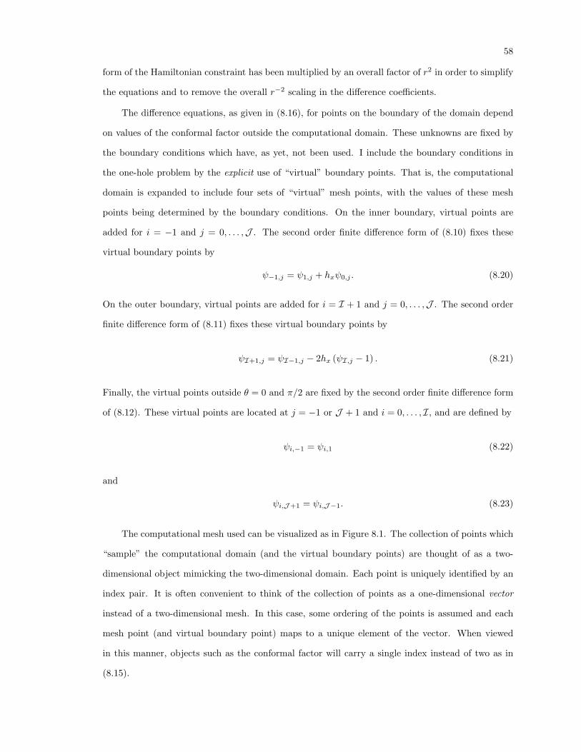
58

form of the Hamiltonian constraint has been multiplied by an overall factor of r2 in order to simplify

the equations and to remove the overall r−2 scaling in the difference coefficients.

The difference equations, as given in (8.16), for points on the boundary of the domain depend

on values of the conformal factor outside the computational domain. These unknowns are fixed by

the boundary conditions which have, as yet, not been used. I include the boundary conditions in

the one-hole problem by the explicit use of “virtual” boundary points. That is, the computational

domain is expanded to include four sets of “virtual” mesh points, with the values of these mesh

points being determined by the boundary conditions. On the inner boundary, virtual points are

added for i = −1 and j = 0, . . . ,J . The second order finite difference form of (8.10) fixes these

virtual boundary points by

ψ−1,j = ψ1,j + hxψ0,j . (8.20)

On the outer boundary, virtual points are added for i = I + 1 and j = 0, . . . ,J . The second order

finite difference form of (8.11) fixes these virtual boundary points by

ψI+1,j = ψI−1,j − 2hx (ψI,j − 1) . (8.21)

Finally, the virtual points outside θ = 0 and π/2 are fixed by the second order finite difference form

of (8.12). These virtual points are located at j = −1 or J + 1 and i = 0, . . . , I, and are defined by

ψi,−1 = ψi,1 (8.22)

and

ψi,J+1 = ψi,J−1. (8.23)

The computational mesh used can be visualized as in Figure 8.1. The collection of points which

“sample” the computational domain (and the virtual boundary points) are thought of as a two-

dimensional object mimicking the two-dimensional domain. Each point is uniquely identified by an

index pair. It is often convenient to think of the collection of points as a one-dimensional vector

instead of a two-dimensional mesh. In this case, some ordering of the points is assumed and each

mesh point (and virtual boundary point) maps to a unique element of the vector. When viewed

in this manner, objects such as the conformal factor will carry a single index instead of two as in

(8.15).

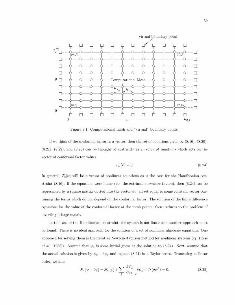
59

0

θ

π/2

0 x xf

(0,0) (I,0)

(0,J ) (I,J )

hθ hx

Computational Mesh

virtual boundary point

1Figure 8.1: Computational mesh and “virtual” boundary points.

If we think of the conformal factor as a vector, then the set of equations given by (8.16), (8.20),

(8.21), (8.22), and (8.23) can be thought of abstractly as a vector of equations which acts on the

vector of conformal factor values

Fa [ψ] = 0. (8.24)

In general, Fa[ψ] will be a vector of nonlinear equations as is the case for the Hamiltonian con-

straint (8.16). If the equations were linear (i.e. the extrinsic curvature is zero), then (8.24) can be

represented by a square matrix dotted into the vector ψa, all set equal to some constant vector con-

taining the terms which do not depend on the conformal factor. The solution of the finite difference

equations for the value of the conformal factor at the mesh points, then, reduces to the problem of

inverting a large matrix.

In the case of the Hamiltonian constraint, the system is not linear and another approach must

be found. There is no ideal approach for the solution of a set of nonlinear algebraic equations. One

approach for solving them is the iterative Newton-Raphson method for nonlinear systems (cf. Press

et al. [1988]). Assume that ψa is some initial guess at the solution to (8.24). Next, assume that

the actual solution is given by ψa + δψa and expand (8.24) in a Taylor series. Truncating at linear

order, we find

Fa [ψ + δψ] = Fa [ψ] +∑b

∂Fa∂ψb

∣∣∣∣ψ

δψb +O(δψ2

)= 0. (8.25)

60

If we define the linearized coefficient matrix Lab as

Lab ≡∂Fa∂ψb

∣∣∣∣ψ

(8.26)

and the “residual” vector Ra as

Ra ≡ −Fa [ψ] , (8.27)

then the solution, δψa, of the linearized equation

∑b

Labδψb = Ra (8.28)

gives a first-order accurate correction to the initial guess ψa. Updating the initial guess (ψa →

ψa + δψa) and iterating until the correction becomes negligible everywhere will (in the absence

of pathological sets of equations) yield a solution to the nonlinear equations (8.24) to any desired

accuracy.

Direct solutions of the difference equations (i.e., those which directly invert the coefficient or

linearized coefficient matrix) are the preferred method of solving the finite difference equations

whenever it is possible. It is often the case, however, that the coefficient matrix is too large and

requires too much computer memory to be directly inverted. If this is the case, other approximation

methods can be used such as simultaneous over-relaxation (SOR), alternating direction implicit

(ADI), conjugate gradient (CG), and many others (cf. Press et al. [1988] or Ames [1977]). All

such approximation schemes iteratively converge to the solution which would be found by a “direct”

solution. The advantages of one over another deal with rates of convergence, computational efficiency,

and the requirement of specific symmetries in the coefficient matrix. Perhaps the most efficient

method for solving the difference equations is the multigrid (MG) approach. The use of this method

for solving the Hamiltonian constraint has been discussed in Choptuik [1982], Choptuik and Unruh

[1986], and Cook [1989]. I have used the MG approach for the solution of the finite difference

equations in the case of a single hole. The details of the MG method are left to Appendix A and

the references therein.

Given a solution to the finite difference form of the Hamiltonian constraint, it is important to

extract any physically significant information about the initial data. Of fundamental interest is the

total ADM energy of the initial slice defined by (7.9). In terms of the conformal factor and using

gravitational units, this becomes

E = − 12π

∮∞Diψd2Si. (8.29)

61

This is not, however, the best form to use for computing the total energy. First, we recall that the

computational domain does not extend to infinity and so this integral must be approximated by the

integral over the outer boundary at a finite radius. Second, evaluating (8.29) from numerical data

will require that a numerical derivative be computed in order to evaluate the integrand. Such a

numerical derivative would necessarily add error to the evaluation of (8.29). An alternate method

for evaluating the total energy (cf. Bowen and York [1980]) can be derived by applying Gauss’ law

to (8.29). The result is

E =1

2π

∮r=a

Diψd2Si −1

2π

∫r>a

∇2ψd3V

=1

4π

∮r=a

ψ

rd2S +

116π

∫r>a

ψ−7AijAijd3V ,

(8.30)

where the Hamiltonian constraint (4.8) and the inner boundary condition (7.2) have been used. (Note

that the unit normal for the surface integral over the inner boundary points out of the domain, i.e.

toward the origin.)

This form for the total energy is much superior to (8.29). The computational approximation

of a finite domain, however, means that the volume integral in (8.30) will be cut off radially at

the outer boundary. Because the integrand falls off as O(r−2), the error in having a finite outer

boundary will, nonetheless, be small if the boundary is far enough out. The major portion of the

energy results from the surface integral and the inner regions of the volume integral. In terms of

the coordinate system being used and in the case of axisymmetry, the total energy can be written

in dimensionless form as

E

a∼=

12

θ=π∫θ=0

ψ(x=0) sin θdθ +18

θ=π∫θ=0

x=xf∫x=0

ψ−7(a2AijA

ij)e3xdxdθ. (8.31)

After computing the total energy, one might consider computing the higher order moments in

the multipole expansion. Because of the reflection symmetry through θ = π/2, the dipole moment

vanishes identically. While higher moments will not vanish identically, it is not clear as to the

usefulness of these quantities and they have not been calculated. A quantity that is of interest is

the area of the throat or minimal surface in the physical space. This quantity is defined as

AMS =∮r=a

ψ4d2S. (8.32)

Associated with the area of the minimal surface is a mass defined similarly to irreducible mass by

M =

√A

16π. (8.33)

62

In terms of the coordinate system being used and in the case of axisymmetry, the area of the

minimal surface can be written in dimensionless form as

AMS

a2= 2π

θ=π∫θ=0

ψ4(x=0) sin θdθ. (8.34)

A code was constructed to solve the finite difference equations described above using the multi-

grid algorithm described in Appendix A. After obtaining a solution, the total energy and minimal

surface area and mass are integrated numerically. In order to test the accuracy of the code, use was

made of an exact solution to a fully non-linear “model” Hamiltonian constraint found by Bowen and

York [1980]. The model problem is obtained by considering a non-physical, spherically symmetric

extrinsic curvature whose square is given by

a2ATijATij = 24

(P

a

)2

e−6xsinh2x. (8.35)

The solution to the model problem is

ψmodel = e−x/2[6 + 2 cosh 2x+ 4

(E

a

)coshx

]1/4

, (8.36)

whereE

a=

√4 +

(P

a

)2

. (8.37)

From (8.34), the area of the minimal surface in the model problem is

Amodel

a2= 16π

(2 +

E

a

)(8.38)

and the mass isMmodel

a=

√2 +

E

a. (8.39)

The code was run using (8.35) for a series of values of the momentum and using the same

computational domain as was used later for the physical problem. Specifically, the outer boundary

was set at x = 10. The radial discretization parameter was set at I = 1024 and the angular parameter

at J = 384 on the finest grid used in the multigrid solution. Table 8.1 below summarizes the results

of the computer solution compared with the exact solution. Full details on the multigrid solutions

to the model problem as well as the physical problem can be found in Appendix B. The computed

solution has proven to be accurate to roughly one part in 10,000 for all examined quantities.

Physical initial-data sets were generated with the same code using (8.7), (8.8), and (8.9) for the

square of the extrinsic curvature. The same computational domain and discretization were used for

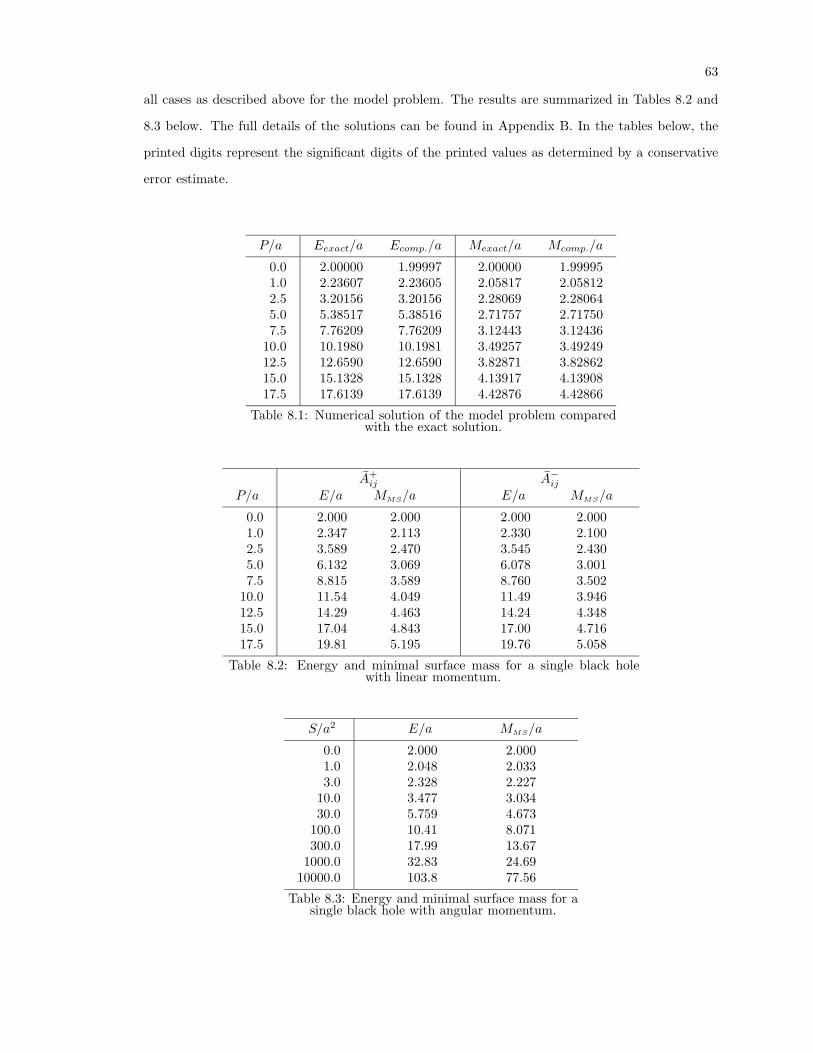
63

all cases as described above for the model problem. The results are summarized in Tables 8.2 and

8.3 below. The full details of the solutions can be found in Appendix B. In the tables below, the

printed digits represent the significant digits of the printed values as determined by a conservative

error estimate.

P/a Eexact/a Ecomp./a Mexact/a Mcomp./a

0.0 2.00000 1.99997 2.00000 1.999951.0 2.23607 2.23605 2.05817 2.058122.5 3.20156 3.20156 2.28069 2.280645.0 5.38517 5.38516 2.71757 2.717507.5 7.76209 7.76209 3.12443 3.12436

10.0 10.1980 10.1981 3.49257 3.4924912.5 12.6590 12.6590 3.82871 3.8286215.0 15.1328 15.1328 4.13917 4.1390817.5 17.6139 17.6139 4.42876 4.42866

Table 8.1: Numerical solution of the model problem comparedwith the exact solution.

A+ij A−ij

P/a E/a MMS/a E/a MMS/a

0.0 2.000 2.000 2.000 2.0001.0 2.347 2.113 2.330 2.1002.5 3.589 2.470 3.545 2.4305.0 6.132 3.069 6.078 3.0017.5 8.815 3.589 8.760 3.502

10.0 11.54 4.049 11.49 3.94612.5 14.29 4.463 14.24 4.34815.0 17.04 4.843 17.00 4.71617.5 19.81 5.195 19.76 5.058

Table 8.2: Energy and minimal surface mass for a single black holewith linear momentum.

S/a2 E/a MMS/a

0.0 2.000 2.0001.0 2.048 2.0333.0 2.328 2.227

10.0 3.477 3.03430.0 5.759 4.673

100.0 10.41 8.071300.0 17.99 13.67

1000.0 32.83 24.6910000.0 103.8 77.56

Table 8.3: Energy and minimal surface mass for asingle black hole with angular momentum.

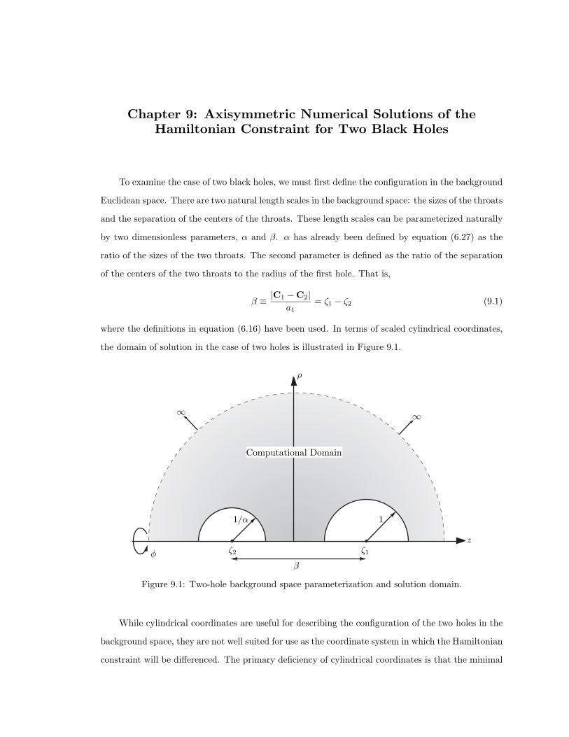
Chapter 9: Axisymmetric Numerical Solutions of theHamiltonian Constraint for Two Black Holes

To examine the case of two black holes, we must first define the configuration in the background

Euclidean space. There are two natural length scales in the background space: the sizes of the throats

and the separation of the centers of the throats. These length scales can be parameterized naturally

by two dimensionless parameters, α and β. α has already been defined by equation (6.27) as the

ratio of the sizes of the two throats. The second parameter is defined as the ratio of the separation

of the centers of the two throats to the radius of the first hole. That is,

β ≡ |C1 −C2|a1

= ζ1 − ζ2 (9.1)

where the definitions in equation (6.16) have been used. In terms of scaled cylindrical coordinates,

the domain of solution in the case of two holes is illustrated in Figure 9.1.

ρ

z

φ

β

ζ1ζ2

11/α

∞ ∞

Computational Domain

1Figure 9.1: Two-hole background space parameterization and solution domain.

While cylindrical coordinates are useful for describing the configuration of the two holes in the

background space, they are not well suited for use as the coordinate system in which the Hamiltonian

constraint will be differenced. The primary deficiency of cylindrical coordinates is that the minimal

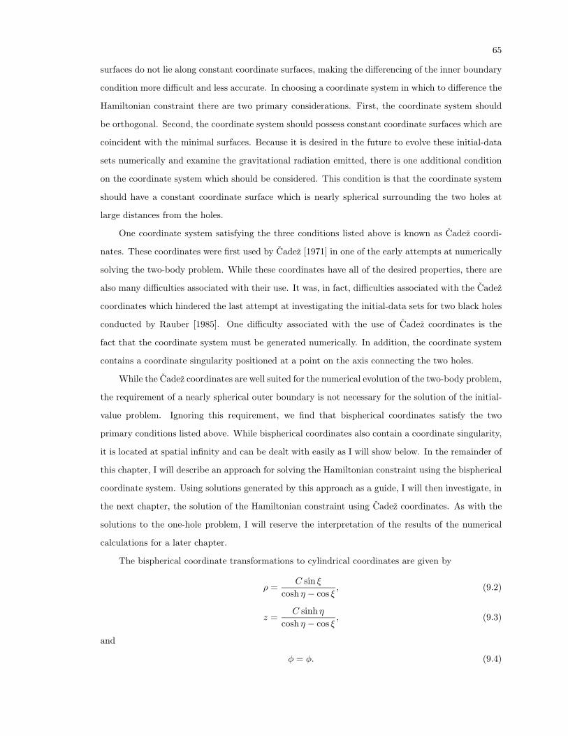
65

surfaces do not lie along constant coordinate surfaces, making the differencing of the inner boundary

condition more difficult and less accurate. In choosing a coordinate system in which to difference the

Hamiltonian constraint there are two primary considerations. First, the coordinate system should

be orthogonal. Second, the coordinate system should possess constant coordinate surfaces which are

coincident with the minimal surfaces. Because it is desired in the future to evolve these initial-data

sets numerically and examine the gravitational radiation emitted, there is one additional condition

on the coordinate system which should be considered. This condition is that the coordinate system

should have a constant coordinate surface which is nearly spherical surrounding the two holes at

large distances from the holes.

One coordinate system satisfying the three conditions listed above is known as Cadez coordi-

nates. These coordinates were first used by Cadez [1971] in one of the early attempts at numerically

solving the two-body problem. While these coordinates have all of the desired properties, there are

also many difficulties associated with their use. It was, in fact, difficulties associated with the Cadez

coordinates which hindered the last attempt at investigating the initial-data sets for two black holes

conducted by Rauber [1985]. One difficulty associated with the use of Cadez coordinates is the

fact that the coordinate system must be generated numerically. In addition, the coordinate system

contains a coordinate singularity positioned at a point on the axis connecting the two holes.

While the Cadez coordinates are well suited for the numerical evolution of the two-body problem,

the requirement of a nearly spherical outer boundary is not necessary for the solution of the initial-

value problem. Ignoring this requirement, we find that bispherical coordinates satisfy the two

primary conditions listed above. While bispherical coordinates also contain a coordinate singularity,

it is located at spatial infinity and can be dealt with easily as I will show below. In the remainder of

this chapter, I will describe an approach for solving the Hamiltonian constraint using the bispherical

coordinate system. Using solutions generated by this approach as a guide, I will then investigate, in

the next chapter, the solution of the Hamiltonian constraint using Cadez coordinates. As with the

solutions to the one-hole problem, I will reserve the interpretation of the results of the numerical

calculations for a later chapter.

The bispherical coordinate transformations to cylindrical coordinates are given by

ρ =C sin ξ

cosh η − cos ξ, (9.2)

z =C sinh η

cosh η − cos ξ, (9.3)

and

φ = φ. (9.4)

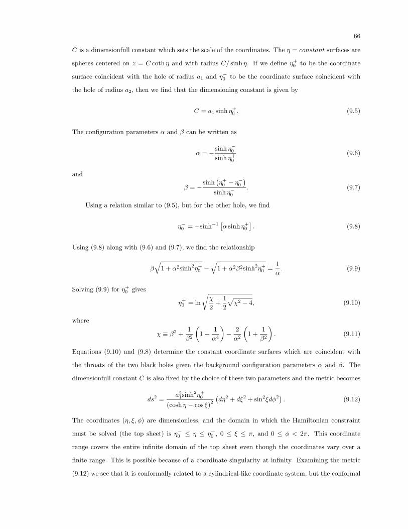
66

C is a dimensionfull constant which sets the scale of the coordinates. The η = constant surfaces are

spheres centered on z = C coth η and with radius C/ sinh η. If we define η+0 to be the coordinate

surface coincident with the hole of radius a1 and η−0 to be the coordinate surface coincident with

the hole of radius a2, then we find that the dimensioning constant is given by

C = a1 sinh η+0 . (9.5)

The configuration parameters α and β can be written as

α = − sinh η−0sinh η+

0

(9.6)

and

β = −sinh

(η+

0 − η−0

)sinh η−0

. (9.7)

Using a relation similar to (9.5), but for the other hole, we find

η−0 = −sinh−1[α sinh η+

0

]. (9.8)

Using (9.8) along with (9.6) and (9.7), we find the relationship

β

√1 + α2sinh2η+

0 −√

1 + α2β2sinh2η+0 =

1α. (9.9)

Solving (9.9) for η+0 gives

η+0 = ln

√χ

2+

12

√χ2 − 4, (9.10)

where

χ ≡ β2 +1β2

(1 +

1α4

)− 2α2

(1 +

1β2

). (9.11)

Equations (9.10) and (9.8) determine the constant coordinate surfaces which are coincident with

the throats of the two black holes given the background configuration parameters α and β. The

dimensionfull constant C is also fixed by the choice of these two parameters and the metric becomes

ds2 =a2

1sinh2η+0

(cosh η − cos ξ)2

(dη2 + dξ2 + sin2ξdφ2

). (9.12)

The coordinates (η, ξ, φ) are dimensionless, and the domain in which the Hamiltonian constraint

must be solved (the top sheet) is η−0 ≤ η ≤ η+0 , 0 ≤ ξ ≤ π, and 0 ≤ φ < 2π. This coordinate

range covers the entire infinite domain of the top sheet even though the coordinates vary over a

finite range. This is possible because of a coordinate singularity at infinity. Examining the metric

(9.12) we see that it is conformally related to a cylindrical-like coordinate system, but the conformal

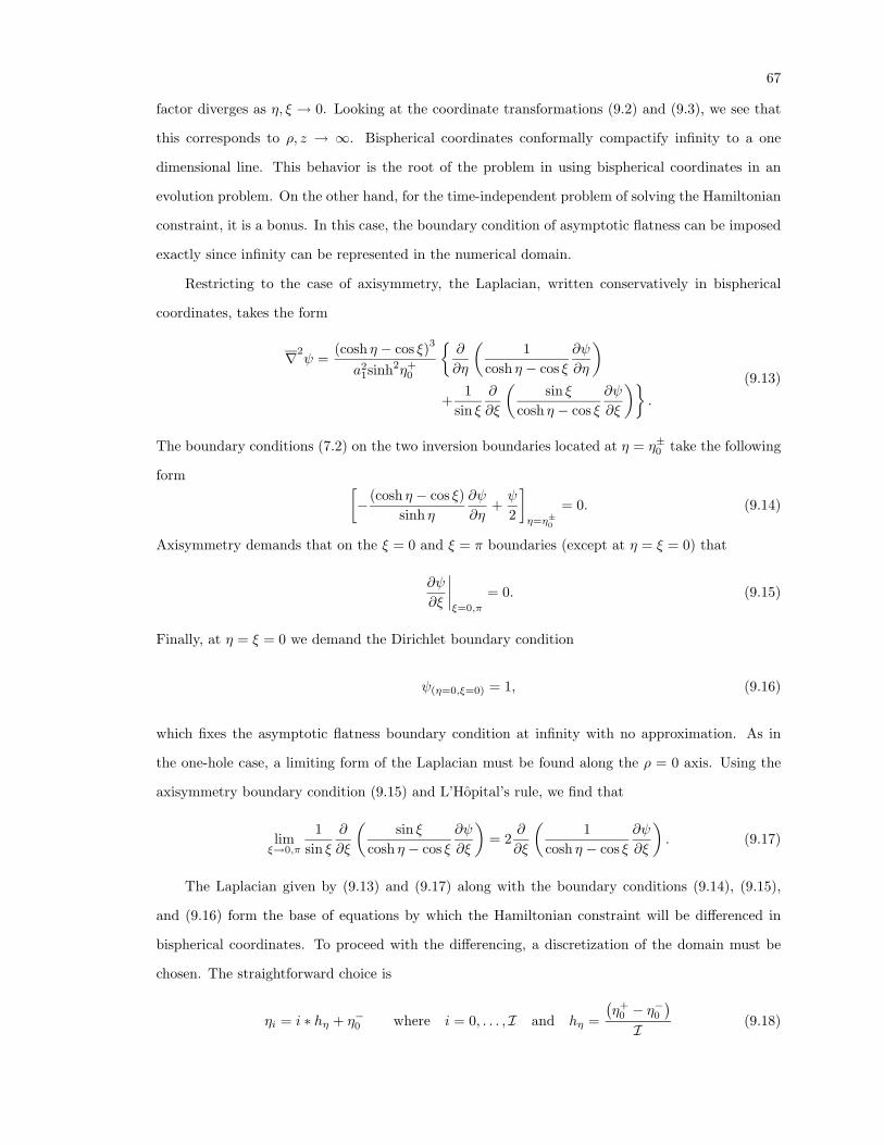
67

factor diverges as η, ξ → 0. Looking at the coordinate transformations (9.2) and (9.3), we see that

this corresponds to ρ, z → ∞. Bispherical coordinates conformally compactify infinity to a one

dimensional line. This behavior is the root of the problem in using bispherical coordinates in an

evolution problem. On the other hand, for the time-independent problem of solving the Hamiltonian

constraint, it is a bonus. In this case, the boundary condition of asymptotic flatness can be imposed

exactly since infinity can be represented in the numerical domain.

Restricting to the case of axisymmetry, the Laplacian, written conservatively in bispherical

coordinates, takes the form

∇2ψ =

(cosh η − cos ξ)3

a21sinh2η+

0

∂

∂η

(1

cosh η − cos ξ∂ψ

∂η

)+

1sin ξ

∂

∂ξ

(sin ξ

cosh η − cos ξ∂ψ

∂ξ

).

(9.13)

The boundary conditions (7.2) on the two inversion boundaries located at η = η±0 take the following

form [− (cosh η − cos ξ)

sinh η∂ψ

∂η+ψ

2

]η=η±0

= 0. (9.14)

Axisymmetry demands that on the ξ = 0 and ξ = π boundaries (except at η = ξ = 0) that

∂ψ

∂ξ

∣∣∣∣ξ=0,π

= 0. (9.15)

Finally, at η = ξ = 0 we demand the Dirichlet boundary condition

ψ(η=0,ξ=0) = 1, (9.16)

which fixes the asymptotic flatness boundary condition at infinity with no approximation. As in

the one-hole case, a limiting form of the Laplacian must be found along the ρ = 0 axis. Using the

axisymmetry boundary condition (9.15) and L’Hopital’s rule, we find that

limξ→0,π

1sin ξ

∂

∂ξ

(sin ξ

cosh η − cos ξ∂ψ

∂ξ

)= 2

∂

∂ξ

(1

cosh η − cos ξ∂ψ

∂ξ

). (9.17)

The Laplacian given by (9.13) and (9.17) along with the boundary conditions (9.14), (9.15),

and (9.16) form the base of equations by which the Hamiltonian constraint will be differenced in

bispherical coordinates. To proceed with the differencing, a discretization of the domain must be

chosen. The straightforward choice is

ηi = i ∗ hη + η−0 where i = 0, . . . , I and hη =

(η+

0 − η−0

)I

(9.18)

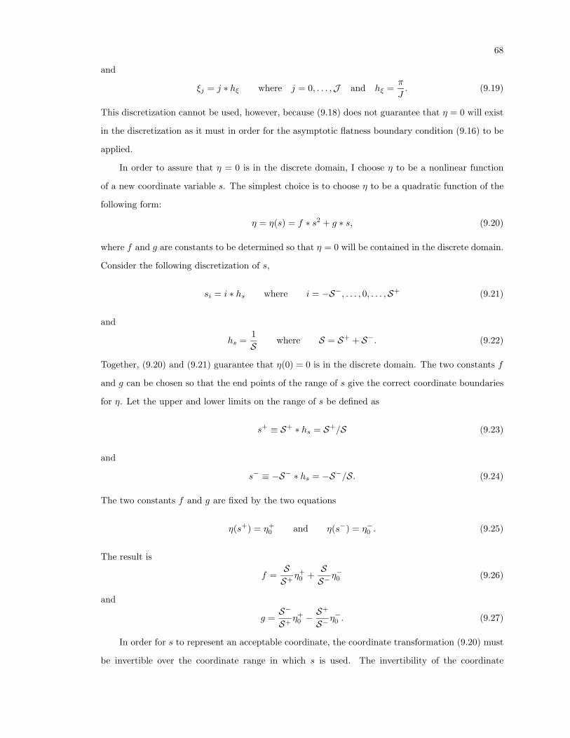
68

and

ξj = j ∗ hξ where j = 0, . . . ,J and hξ =π

J. (9.19)

This discretization cannot be used, however, because (9.18) does not guarantee that η = 0 will exist

in the discretization as it must in order for the asymptotic flatness boundary condition (9.16) to be

applied.

In order to assure that η = 0 is in the discrete domain, I choose η to be a nonlinear function

of a new coordinate variable s. The simplest choice is to choose η to be a quadratic function of the

following form:

η = η(s) = f ∗ s2 + g ∗ s, (9.20)

where f and g are constants to be determined so that η = 0 will be contained in the discrete domain.

Consider the following discretization of s,

si = i ∗ hs where i = −S−, . . . , 0, . . . ,S+ (9.21)

and

hs =1S

where S = S+ + S−. (9.22)

Together, (9.20) and (9.21) guarantee that η(0) = 0 is in the discrete domain. The two constants f

and g can be chosen so that the end points of the range of s give the correct coordinate boundaries

for η. Let the upper and lower limits on the range of s be defined as

s+ ≡ S+ ∗ hs = S+/S (9.23)

and

s− ≡ −S− ∗ hs = −S−/S. (9.24)

The two constants f and g are fixed by the two equations

η(s+) = η+0 and η(s−) = η−0 . (9.25)

The result is

f =SS+

η+0 +

SS−

η−0 (9.26)

and

g =S−

S+η+

0 −S+

S−η−0 . (9.27)

In order for s to represent an acceptable coordinate, the coordinate transformation (9.20) must

be invertible over the coordinate range in which s is used. The invertibility of the coordinate

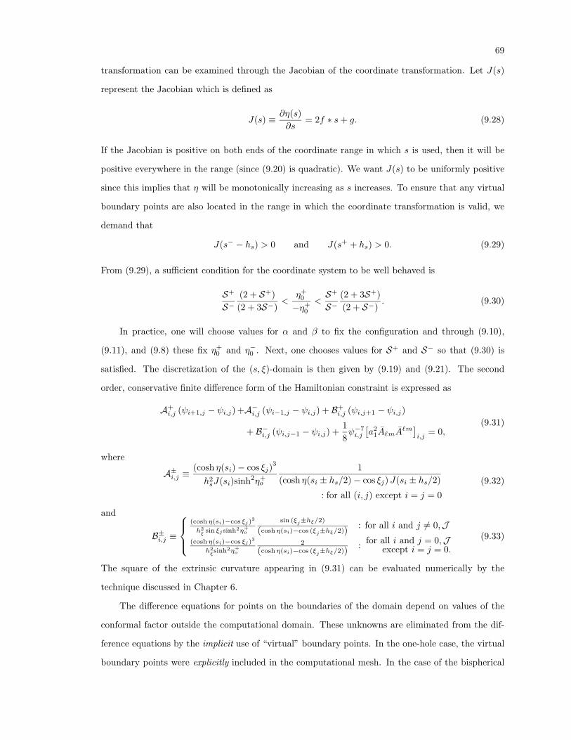
69

transformation can be examined through the Jacobian of the coordinate transformation. Let J(s)

represent the Jacobian which is defined as

J(s) ≡ ∂η(s)∂s

= 2f ∗ s+ g. (9.28)

If the Jacobian is positive on both ends of the coordinate range in which s is used, then it will be

positive everywhere in the range (since (9.20) is quadratic). We want J(s) to be uniformly positive

since this implies that η will be monotonically increasing as s increases. To ensure that any virtual

boundary points are also located in the range in which the coordinate transformation is valid, we

demand that

J(s− − hs) > 0 and J(s+ + hs) > 0. (9.29)

From (9.29), a sufficient condition for the coordinate system to be well behaved is

S+

S−(2 + S+)(2 + 3S−)

<η+

0

−η+0

<S+

S−(2 + 3S+)(2 + S−)

. (9.30)

In practice, one will choose values for α and β to fix the configuration and through (9.10),

(9.11), and (9.8) these fix η+0 and η−0 . Next, one chooses values for S+ and S− so that (9.30) is

satisfied. The discretization of the (s, ξ)-domain is then given by (9.19) and (9.21). The second

order, conservative finite difference form of the Hamiltonian constraint is expressed as

A+i,j (ψi+1,j − ψi,j) +A−i,j (ψi−1,j − ψi,j) + B+

i,j (ψi,j+1 − ψi,j)

+ B−i,j (ψi,j−1 − ψi,j) +18ψ−7i,j

[a2

1A`mA`m]i,j

= 0,(9.31)

where

A±i,j ≡(cosh η(si)− cos ξj)

3

h2sJ(si)sinh2η+

o

1(cosh η(si ± hs/2)− cos ξj) J(si ± hs/2)

: for all (i, j) except i = j = 0

(9.32)

and

B±i,j ≡

(cosh η(si)−cos ξj)

3

h2ξ

sin ξjsinh2η+o

sin (ξj±hξ/2)

(cosh η(si)−cos (ξj±hξ/2)) : for all i and j 6= 0,J(cosh η(si)−cos ξj)

3

h2ξsinh2η+

o

2

(cosh η(si)−cos (ξj±hξ/2)) : for all i and j = 0,Jexcept i = j = 0.

(9.33)

The square of the extrinsic curvature appearing in (9.31) can be evaluated numerically by the

technique discussed in Chapter 6.

The difference equations for points on the boundaries of the domain depend on values of the

conformal factor outside the computational domain. These unknowns are eliminated from the dif-

ference equations by the implicit use of “virtual” boundary points. In the one-hole case, the virtual

boundary points were explicitly included in the computational mesh. In the case of the bispherical

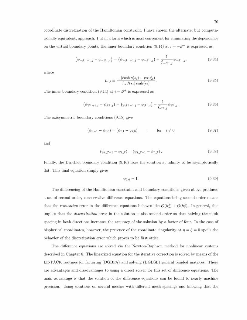
70

coordinate discretization of the Hamiltonian constraint, I have chosen the alternate, but computa-

tionally equivalent, approach. Put in a form which is most convenient for eliminating the dependence

on the virtual boundary points, the inner boundary condition (9.14) at i = −S− is expressed as

(ψ−S−−1,j − ψ−S−,j

)=(ψ−S−+1,j − ψ−S−,j

)+

1C−S−,j

ψ−S−,j , (9.34)

where

Ci,j ≡− (cosh η(si)− cos ξj)

hsJ(si) sinh(si). (9.35)

The inner boundary condition (9.14) at i = S+ is expressed as

(ψS++1,j − ψS+,j

)=(ψS+−1,j − ψS+,j

)− 1CS+,j

ψS+,j . (9.36)

The axisymmetric boundary conditions (9.15) give

(ψi,−1 − ψi,0) = (ψi,1 − ψi,0) : for i 6= 0 (9.37)

and

(ψi,J+1 − ψi,J ) = (ψi,J−1 − ψi,J ) . (9.38)

Finally, the Dirichlet boundary condition (9.16) fixes the solution at infinity to be asymptotically

flat. This final equation simply gives

ψ0,0 = 1. (9.39)

The differencing of the Hamiltonian constraint and boundary conditions given above produces

a set of second order, conservative difference equations. The equations being second order means

that the truncation error in the difference equations behaves like O(h2s) + O(h2

ξ). In general, this

implies that the discretization error in the solution is also second order so that halving the mesh

spacing in both directions increases the accuracy of the solution by a factor of four. In the case of

bispherical coordinates, however, the presence of the coordinate singularity at η = ξ = 0 spoils the

behavior of the discretization error which proves to be first order.

The difference equations are solved via the Newton-Raphson method for nonlinear systems

described in Chapter 8. The linearized equation for the iterative correction is solved by means of the

LINPACK routines for factoring (DGBFA) and solving (DGBSL) general banded matrices. There

are advantages and disadvantages to using a direct solver for this set of difference equations. The

main advantage is that the solution of the difference equations can be found to nearly machine

precision. Using solutions on several meshes with different mesh spacings and knowing that the

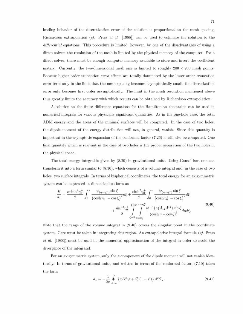
71

leading behavior of the discretization error of the solution is proportional to the mesh spacing,

Richardson extrapolation (cf. Press et al. [1988]) can be used to estimate the solution to the

differential equations. This procedure is limited, however, by one of the disadvantages of using a

direct solver: the resolution of the mesh is limited by the physical memory of the computer. For a

direct solver, there must be enough computer memory available to store and invert the coefficient

matrix. Currently, the two-dimensional mesh size is limited to roughly 200 × 200 mesh points.

Because higher order truncation error effects are totally dominated by the lower order truncation

error term only in the limit that the mesh spacing becomes asymptotically small, the discretization

error only becomes first order asymptotically. The limit in the mesh resolution mentioned above

thus greatly limits the accuracy with which results can be obtained by Richardson extrapolation.

A solution to the finite difference equations for the Hamiltonian constraint can be used in

numerical integrals for various physically significant quantities. As in the one-hole case, the total

ADM energy and the areas of the minimal surfaces will be computed. In the case of two holes,

the dipole moment of the energy distribution will not, in general, vanish. Since this quantity is

important in the asymptotic expansion of the conformal factor (7.26) it will also be computed. One

final quantity which is relevant in the case of two holes is the proper separation of the two holes in

the physical space.

The total energy integral is given by (8.29) in gravitational units. Using Gauss’ law, one can

transform it into a form similar to (8.30), which consists of a volume integral and, in the case of two

holes, two surface integrals. In terms of bispherical coordinates, the total energy for an axisymmetric

system can be expressed in dimensionless form as

E

a1=αsinh2η+

0

2

∫ π

0

ψ(η=η−0 ) sin ξ(cosh η−0 − cos ξ

)2 dξ +sinh2η+

0

2

∫ π

0

ψ(η=η+0 ) sin ξ(

cosh η+0 − cos ξ

)2 dξ+

sinh3η+0

8

ξ=π∫ξ=0

η=η+0∫

η=η−0

ψ−7(a2

1AijAij)

sin ξ

(cosh η − cos ξ)3 dηdξ.

(9.40)

Note that the range of the volume integral in (9.40) covers the singular point in the coordinate

system. Care must be taken in integrating this region. An extrapolative integral formula (cf. Press

et al. [1988]) must be used in the numerical approximation of the integral in order to avoid the

divergence of the integrand.

For an axisymmetric system, only the z-component of the dipole moment will not vanish iden-

tically. In terms of gravitational units, and written in terms of the conformal factor, (7.10) takes

the form

dz = − 12π

∮∞

zDkψ + δkz (1− ψ)

d2Sk. (9.41)

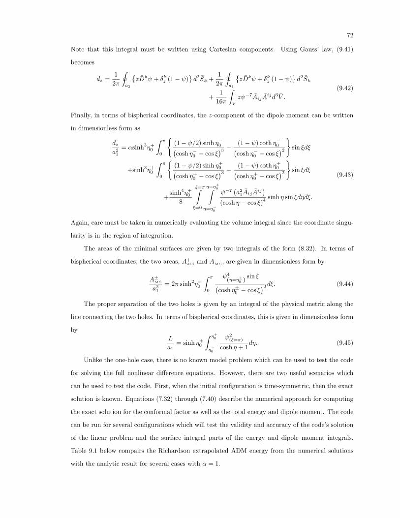
72

Note that this integral must be written using Cartesian components. Using Gauss’ law, (9.41)

becomes

dz =1

2π

∮a2

zDkψ + δkz (1− ψ)

d2Sk +

12π

∮a1

zDkψ + δkz (1− ψ)

d2Sk

+1

16π

∫V

zψ−7AijAijd3V .

(9.42)

Finally, in terms of bispherical coordinates, the z-component of the dipole moment can be written

in dimensionless form as

dza2

1

= αsinh3η+0

∫ π

0

(1− ψ/2) sinh η−0(cosh η−0 − cos ξ

)3 − (1− ψ) coth η−0(cosh η−0 − cos ξ

)2

sin ξdξ

+sinh3η+0

∫ π

0

(1− ψ/2) sinh η+

0(cosh η+

0 − cos ξ)3 − (1− ψ) coth η+

0(cosh η+

0 − cos ξ)2

sin ξdξ

+sinh4η+

0

8

ξ=π∫ξ=0

η=η+0∫

η=η−0

ψ−7(a2

1AijAij)

(cosh η − cos ξ)4 sinh η sin ξdηdξ.

(9.43)

Again, care must be taken in numerically evaluating the volume integral since the coordinate singu-

larity is in the region of integration.

The areas of the minimal surfaces are given by two integrals of the form (8.32). In terms of

bispherical coordinates, the two areas, A+MS and A−MS, are given in dimensionless form by

A±MSa2

1

= 2π sinh2η+0

∫ π

0

ψ4

(η=η±0 ) sin ξ(cosh η±0 − cos ξ

)2 dξ. (9.44)

The proper separation of the two holes is given by an integral of the physical metric along the

line connecting the two holes. In terms of bispherical coordinates, this is given in dimensionless form

byL

a1= sinh η+

0

∫ η+0

η−0

ψ2(ξ=π)

cosh η + 1dη. (9.45)

Unlike the one-hole case, there is no known model problem which can be used to test the code

for solving the full nonlinear difference equations. However, there are two useful scenarios which

can be used to test the code. First, when the initial configuration is time-symmetric, then the exact

solution is known. Equations (7.32) through (7.40) describe the numerical approach for computing

the exact solution for the conformal factor as well as the total energy and dipole moment. The code

can be run for several configurations which will test the validity and accuracy of the code’s solution

of the linear problem and the surface integral parts of the energy and dipole moment integrals.

Table 9.1 below compairs the Richardson extrapolated ADM energy from the numerical solutions

with the analytic result for several cases with α = 1.

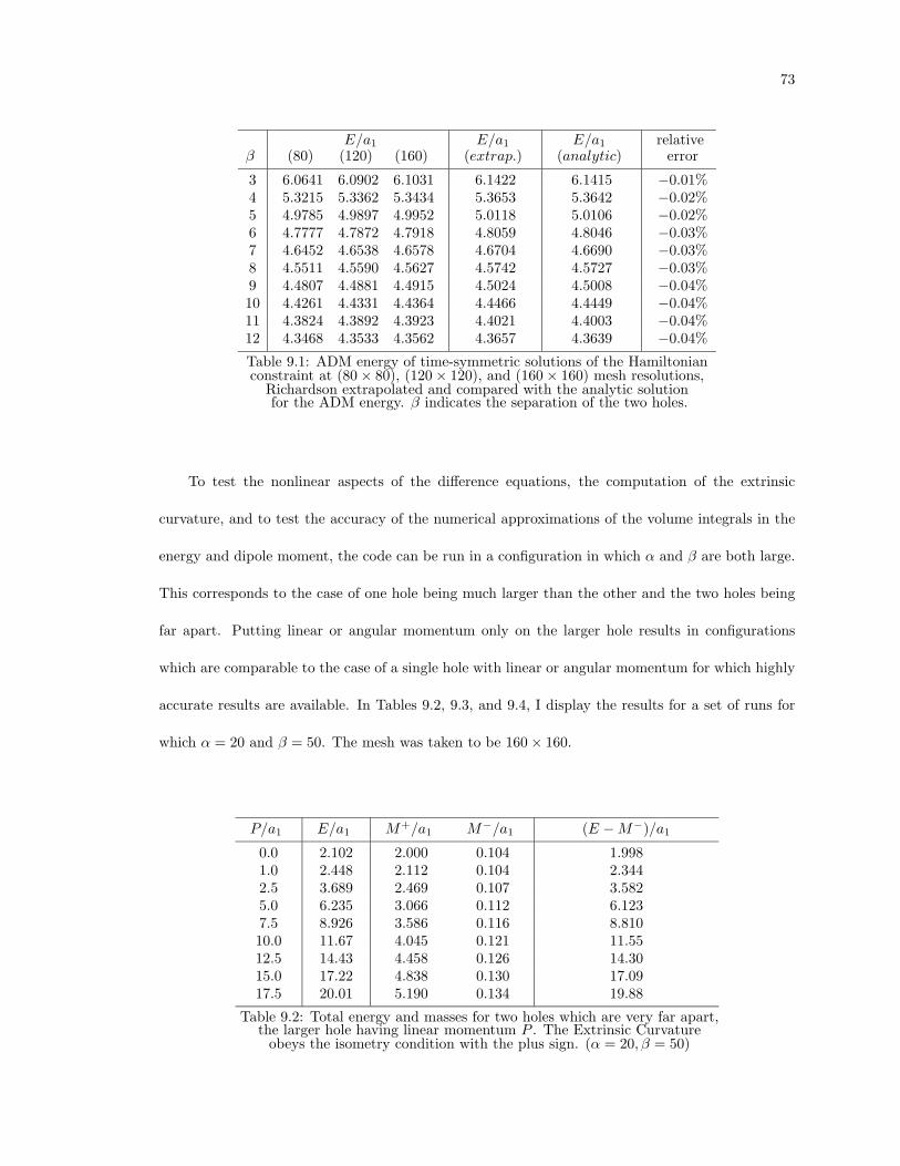
73

E/a1 E/a1 E/a1 relativeβ (80) (120) (160) (extrap.) (analytic) error

3 6.0641 6.0902 6.1031 6.1422 6.1415 −0.01%4 5.3215 5.3362 5.3434 5.3653 5.3642 −0.02%5 4.9785 4.9897 4.9952 5.0118 5.0106 −0.02%6 4.7777 4.7872 4.7918 4.8059 4.8046 −0.03%7 4.6452 4.6538 4.6578 4.6704 4.6690 −0.03%8 4.5511 4.5590 4.5627 4.5742 4.5727 −0.03%9 4.4807 4.4881 4.4915 4.5024 4.5008 −0.04%10 4.4261 4.4331 4.4364 4.4466 4.4449 −0.04%11 4.3824 4.3892 4.3923 4.4021 4.4003 −0.04%12 4.3468 4.3533 4.3562 4.3657 4.3639 −0.04%

Table 9.1: ADM energy of time-symmetric solutions of the Hamiltonianconstraint at (80× 80), (120× 120), and (160× 160) mesh resolutions,

Richardson extrapolated and compared with the analytic solutionfor the ADM energy. β indicates the separation of the two holes.

To test the nonlinear aspects of the difference equations, the computation of the extrinsic

curvature, and to test the accuracy of the numerical approximations of the volume integrals in the

energy and dipole moment, the code can be run in a configuration in which α and β are both large.

This corresponds to the case of one hole being much larger than the other and the two holes being

far apart. Putting linear or angular momentum only on the larger hole results in configurations

which are comparable to the case of a single hole with linear or angular momentum for which highly

accurate results are available. In Tables 9.2, 9.3, and 9.4, I display the results for a set of runs for

which α = 20 and β = 50. The mesh was taken to be 160× 160.

P/a1 E/a1 M+/a1 M−/a1 (E −M−)/a1

0.0 2.102 2.000 0.104 1.9981.0 2.448 2.112 0.104 2.3442.5 3.689 2.469 0.107 3.5825.0 6.235 3.066 0.112 6.1237.5 8.926 3.586 0.116 8.81010.0 11.67 4.045 0.121 11.5512.5 14.43 4.458 0.126 14.3015.0 17.22 4.838 0.130 17.0917.5 20.01 5.190 0.134 19.88

Table 9.2: Total energy and masses for two holes which are very far apart,the larger hole having linear momentum P . The Extrinsic Curvature

obeys the isometry condition with the plus sign. (α = 20, β = 50)

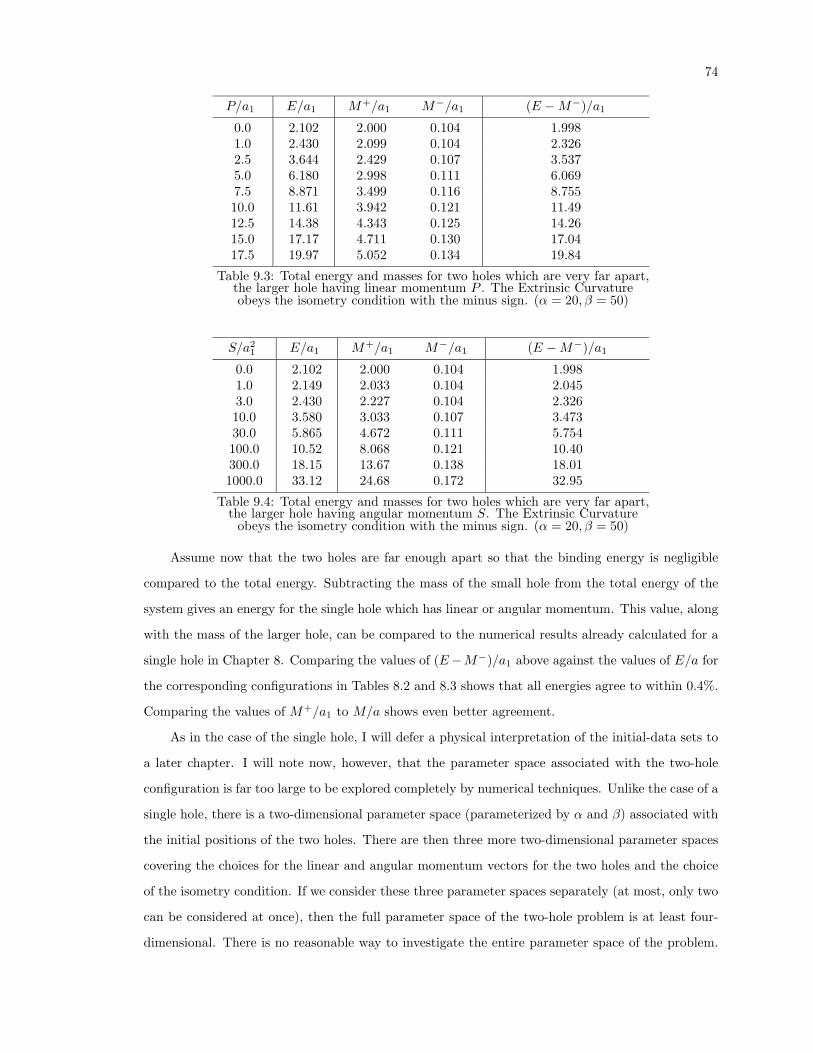
74

P/a1 E/a1 M+/a1 M−/a1 (E −M−)/a1

0.0 2.102 2.000 0.104 1.9981.0 2.430 2.099 0.104 2.3262.5 3.644 2.429 0.107 3.5375.0 6.180 2.998 0.111 6.0697.5 8.871 3.499 0.116 8.75510.0 11.61 3.942 0.121 11.4912.5 14.38 4.343 0.125 14.2615.0 17.17 4.711 0.130 17.0417.5 19.97 5.052 0.134 19.84

Table 9.3: Total energy and masses for two holes which are very far apart,the larger hole having linear momentum P . The Extrinsic Curvatureobeys the isometry condition with the minus sign. (α = 20, β = 50)

S/a21 E/a1 M+/a1 M−/a1 (E −M−)/a1

0.0 2.102 2.000 0.104 1.9981.0 2.149 2.033 0.104 2.0453.0 2.430 2.227 0.104 2.32610.0 3.580 3.033 0.107 3.47330.0 5.865 4.672 0.111 5.754100.0 10.52 8.068 0.121 10.40300.0 18.15 13.67 0.138 18.011000.0 33.12 24.68 0.172 32.95

Table 9.4: Total energy and masses for two holes which are very far apart,the larger hole having angular momentum S. The Extrinsic Curvature

obeys the isometry condition with the minus sign. (α = 20, β = 50)

Assume now that the two holes are far enough apart so that the binding energy is negligible

compared to the total energy. Subtracting the mass of the small hole from the total energy of the

system gives an energy for the single hole which has linear or angular momentum. This value, along

with the mass of the larger hole, can be compared to the numerical results already calculated for a

single hole in Chapter 8. Comparing the values of (E−M−)/a1 above against the values of E/a for

the corresponding configurations in Tables 8.2 and 8.3 shows that all energies agree to within 0.4%.

Comparing the values of M+/a1 to M/a shows even better agreement.

As in the case of the single hole, I will defer a physical interpretation of the initial-data sets to

a later chapter. I will note now, however, that the parameter space associated with the two-hole

configuration is far too large to be explored completely by numerical techniques. Unlike the case of a

single hole, there is a two-dimensional parameter space (parameterized by α and β) associated with

the initial positions of the two holes. There are then three more two-dimensional parameter spaces

covering the choices for the linear and angular momentum vectors for the two holes and the choice

of the isometry condition. If we consider these three parameter spaces separately (at most, only two

can be considered at once), then the full parameter space of the two-hole problem is at least four-

dimensional. There is no reasonable way to investigate the entire parameter space of the problem.

75

The most reasonable approach for exploring the possible configurations is to reduce the size of the

parameter space by only considering configurations with some symmetry. For example, if we consider

only configurations in which the two holes are of equal size, then the parameter space is restricted

to the α = 1 hyperplane. If, in addition, the magnitudes of the linear or angular momenta of the

two holes are equal, then the parameter space is further reduced to two, two-dimensional parameter

spaces corresponding to the cases where the momentum vectors are either parallel or anti-parallel.

With these symmetries, the remaining parameter space can be sampled and the results can be

effectively visualized. The results from an extensive sampling of this reduced parameter space are

tabulated in Appendix C and are discussed in a later chapter.

Chapter 10: The Hamiltonian Constraint for Two BlackHoles Using Cadez Coordinates

As mentioned in Chapter 9, the coordinate system first used by Cadez [1971] in his early inves-

tigations into black-hole collisions is the best coordinate system known at this time for investigating

the numerical evolution of two-hole, initial-data sets. Unfortunately, this coordinate system is dif-

ficult to work with because it must be constructed numerically and because it contains a severe

coordinate singularity. In this chapter, I will describe all aspects of the problem of defining Cadez

coordinates and explore an approach for applying them to the problem of solving the Hamiltonian

constraint for two black holes.

Cadez coordinates are defined in terms of a complex-plane transformation (cf. Moon and Spincer

[1988]). Letting the base coordinate system be cylindrical coordinates, the complex variable ζ is

defined as

ζ ≡ z + iρ. (10.1)

The cylindrical coordinate z is then the real part of ζ and the cylindrical coordinate ρ is the imaginary

part of ζ. The Cadez coordinates are defined as the real and imaginary parts of a complex function

χ(ζ). Specifically,

η(ρ, z) ≡ <eχ(ζ) and ξ(ρ, z) ≡ =mχ(ζ). (10.2)

Defined in this way, the coordinate system is guaranteed to be orthogonal everywhere that χ is

analytic. The explicit form of the complex function χ is taken to be

χ(ζ) ≡ C+0 ln(ζ − ζ+) + C−0 ln(ζ − ζ−) +

∞∑n=1

C+n

(ζ − ζ+

)−n + C−n(ζ − ζ−

)−n. (10.3)

The coefficients C±i are real scalars and the two complex parameters ζ± will fix the locations of the

two holes.

To see the general behavior of this transformation, consider the limit that |ζ| is large compared

to |ζ+| and |ζ−|. In this case, (10.3) becomes

χ(ζ) ≈(C+

0 + C−0)

ln(ζ) (10.4)

77

and the coordinate transformations become

η(ρ, z) ≈(C+

0 + C−0)

ln√ρ2 + z2 (10.5a)

and

ξ(ρ, z) ≈(C+

0 + C−0)

arg(ζ). (10.5b)

We are free to scale the coordinate system so that C+0 + C−0 = 1 and, in this limit, η is simply a

logarithmically scaled, spherical-polar radial coordinate and ξ is simply the spherical-polar colatitude

coordinate. This transition to spherical-polar behavior in the coordinates is precisely the desired

behavior, at large distances from the holes, alluded to in Chapter 9.

If we consider only the logarithmic terms in (10.3) and take the limit that ζ → ζ±, then we find

that the coordinates again approach logarithmically scaled, spherical-polar coordinates, but centered

around ζ±. We see then that the η = constant surfaces near ζ± form ovals surrounding ζ+ and

ζ− and the coefficients in the infinite series in (10.3) can be chosen to make specific η = constant

surfaces truly spherical. This is again the desired behavior, near the holes, for a coordinate system

described in Chapter 9.

The coordinate system based on (10.3) thus has all of the properties desired for a coordinate

system to be used for a two-hole manifold. Previous work (Cadez [1971], Smarr et al. [1976], Rauber

[1985]) done with these coordinates has been restricted to the case in which the two holes are of

equal size. This restriction simplifies the definition of the coordinate system (10.3). Here, however,

I have extended the traditional definition of Cadez coordinates so that it can address problems in

which the holes are not of equal size. The remaining task in defining the Cadez coordinates is to

prescribe a method for fixing the coefficients C±i and parameters ζ±.

As in the case of bispherical coordinates, I parameterize the configuration by the two dimension-

less parameters α and β (cf. Chapter 9). In order to maintain the ability to transform to bispherical

coordinates easily, I choose to locate the boundaries of the holes (throats) as prescribed in Chapter 9

for bispherical coordinates. This approach determines the two bispherical coordinate surfaces η±0

with which the throats are coincident. The two positional parameters ζ± are then fixed as

ζ+ ≡ cosh η+0 and ζ− ≡ α−1 cosh η−0 . (10.6)

In terms of the complex variable ζ, the two sets of points constituting the throats can be parame-

terized by θ± in the following way:

ζ(θ+) ≡ ζ+ + cos θ+ + i sin θ+ for 0 ≤ θ+ ≤ π (10.7)

78

and

ζ(θ−) ≡ ζ− + α−1(cos θ− + i sin θ−

)for 0 ≤ θ− ≤ π. (10.8)

Using (10.7) and (10.8), the C±i coefficients are fixed by demanding that

η+ = <eχ(ζ(θ+)) and η− = <eχ(ζ(θ−)), (10.9)

where η± are the coordinate values of the Cadez coordinate η for each of the throats and these can

be freely chosen (the implications of their choice will be discussed below). The two equations in

(10.9), evaluated at a large set of points on (10.7) and (10.8), yield a large set of equations which

can be used to fix the C±i coefficients numerically by a linear least squares fit. Finally, given values

for the C±i coefficients, they, and the values for η±, are rescaled so that C+0 + C−0 = 1.

Given a point in cylindrical coordinates, the corresponding point in Cadez coordinates is easily

obtained from (10.2). However, given a point χ0 = χ(η, x) in Cadez coordinates, the corresponding

point in cylindrical coordinates can only by found numerically. The inversion can be accomplished

iteratively via Newton’s method generalized for complex functions. The algorithm is

ζi+1 = ζi −(χ(ζi)− χ0

)( ∂χ

∂ζ

∣∣∣∣ζi

)−1

. (10.10)

Because of the behavior demanded in the coordinate system around the throats and at large

distances, there is necessarily a critical point in the complex transformation (10.3). This point is

defined by∂χ(ζ)∂ζ

= 0. (10.11)

Recalling the Cauchy-Riemann conditions

∂η

∂z=∂ξ

∂ρand

∂η

∂ρ= −∂ξ

∂z, (10.12)

the determinant of the Jacobian of the coordinate transformation becomes

J =∂η

∂ρ

∂ξ

∂z− ∂η

∂z

∂ξ

∂ρ= −

(∂η

∂ρ

)2

−(∂η

∂z

)2

= −∣∣∣∣∂χ∂ζ

∣∣∣∣2. (10.13)

Thus, the critical point in (10.3) is a saddle-point singularity of the coordinate system. This singular

point will be located somewhere on the symmetry axis connecting the two throats. The exact location

will be determined by the choices made for the values of η±. In fact, the freedom to choose η± is

used to position the singularity at some desired location.

The location of the singular point must be determined numerically. Having fixed the coefficients

in the definition of (10.3) as describe above, equation (10.11) can be solved iteratively via Newton’s

method generalized for complex functions. The algorithm is

ζi+1s = ζis −

∂χ

∂ζ

∣∣∣∣ζis

(∂2χ

∂ζ2

∣∣∣∣ζis

)−1

, (10.14)

where ζs denotes the singular value of ζ.

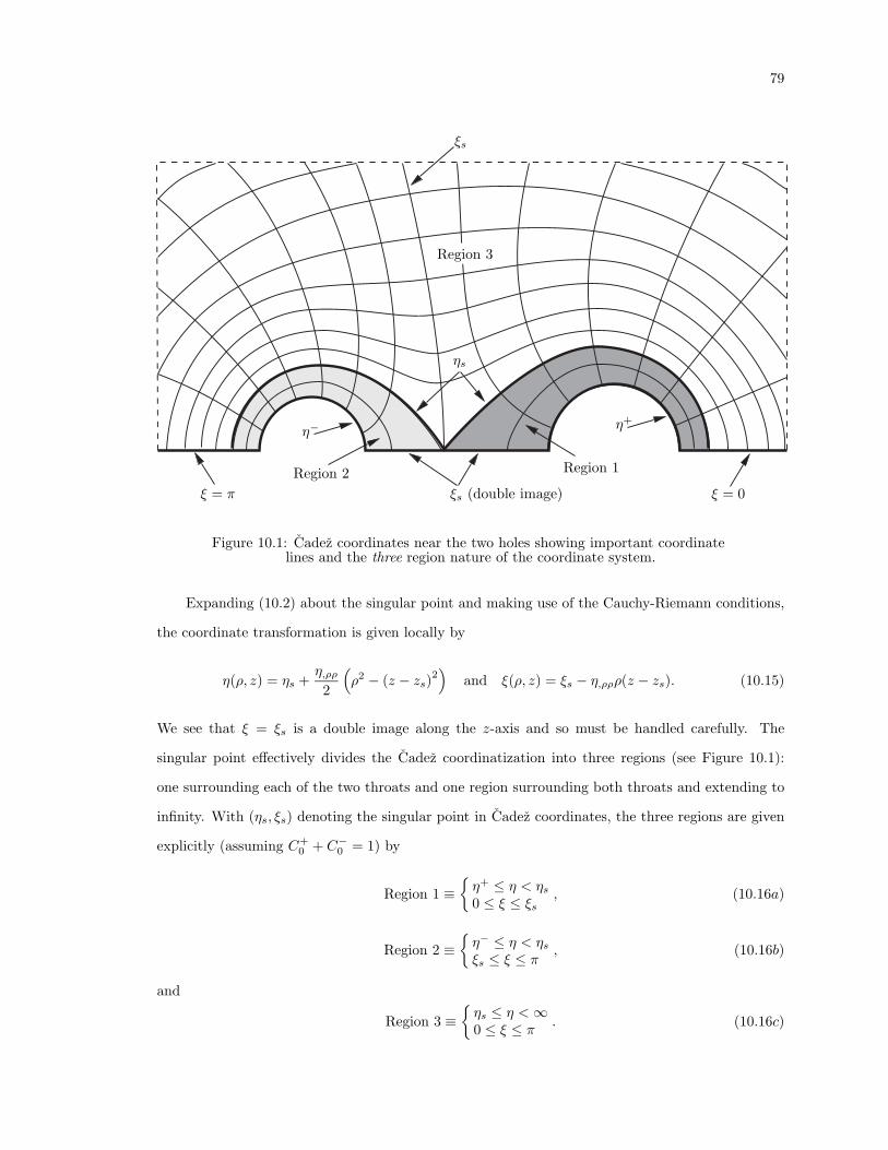
79

η+η−

ηs

ξ = 0ξ = π

ξs

ξs (double image)

Region 1Region 2

Region 3

1Figure 10.1: Cadez coordinates near the two holes showing important coordinatelines and the three region nature of the coordinate system.

Expanding (10.2) about the singular point and making use of the Cauchy-Riemann conditions,

the coordinate transformation is given locally by

η(ρ, z) = ηs +η,ρρ

2

(ρ2 − (z − zs)2

)and ξ(ρ, z) = ξs − η,ρρρ(z − zs). (10.15)

We see that ξ = ξs is a double image along the z-axis and so must be handled carefully. The

singular point effectively divides the Cadez coordinatization into three regions (see Figure 10.1):

one surrounding each of the two throats and one region surrounding both throats and extending to

infinity. With (ηs, ξs) denoting the singular point in Cadez coordinates, the three regions are given

explicitly (assuming C+0 + C−0 = 1) by

Region 1 ≡η+ ≤ η < ηs0 ≤ ξ ≤ ξs

, (10.16a)

Region 2 ≡η− ≤ η < ηsξs ≤ ξ ≤ π

, (10.16b)

and

Region 3 ≡ηs ≤ η <∞0 ≤ ξ ≤ π . (10.16c)

80

The presence of this coordinate singularity places one final restriction on the definition of the

Cadez coordinates. In order to handle the singular point numerically, I will demand that it always

be represented in the discretization of the domain. In order to maintain a constant interval in the

discretization of the η coordinate, it is necessary to demand that

ηs − η+

ηs − η=I+

I−, (10.17)

where I+ and I− are positive integers. This demand can be satisfied iteratively by making initial

guesses for η±, solving for the Cadez coefficients, and determining an initial value for ηs. Next, if

(10.17) is not satisfied, assume η+ → η+ + ε and η− → η− − ε. Inserting these into (10.17) and

solving for ε gives a correction for η±. The new guesses for η± are used to solve again for the Cadez

coefficients and for ηs and the iteration is continued until (10.17) is satisfied. This procedure has

proven to be rapidly convergent.

With the Cadez coordinates fully defined, they can now be applied to the problem of solving the

Hamiltonian constraint. Because of the nature of the coordinate transformations, all quantities are

explicitly functions of the cylindrical coordinates and are functions of the Cadez coordinates only

implicitly through the numerical inverse coordinate transformation. The Jacobian of the coordinate

transformation from cylindrical to Cadez coordinates is given by

Jji =

η,ρ 0 η,z0 1 0η,z 0 −η,ρ

(10.18)

and the inverse Jacobian by

(J−1

)ji

=

η,ρ

(η2,ρ+η2

,z)0 η,z

(η2,ρ+η2

,z)0 1 0η,z

(η2,ρ+η2

,z)0 −η,ρ

(η2,ρ+η2

,z)

. (10.19)

The metric is given by

ds2 =a2

1

η2,ρ + η2

,z

(dη2 + dξ2

)+ a2

1ρ2dφ2, (10.20)

where ρ and z are dimensionless coordinates scaled relative to a1.

The Laplacian can be written in Cadez coordinates by applying the chain rule to the Laplacian

in cylindrical coordinates as done by Rauber [1985]. The Laplacian, in this form, cannot be con-

servatively differenced which is a significant disadvantage to finding numerical solutions. However,

by making use of the explicit form of the inverse Jacobian, the Laplacian can be rewritten in a

form which can be conservatively differenced. Restricting to the case of axisymmetry, the Laplacian,

written conservatively in Cadez coordinates, takes the form

∇2ψ =

η2,ρ + η2

,z

a21ρ

∂

∂η

(ρ∂ψ

∂η

)+

∂

∂ξ

(ρ∂ψ

∂ξ

). (10.21)

81

The boundary conditions (7.2) on the two inversion boundaries located at η = η± take the following

forms, [√η2,ρ + η2

,z

∂ψ

∂η+ψ

2

]η=η+

= 0 (10.22a)

and [√η2,ρ + η2

,z

∂ψ

∂η+αψ

2

]η=η−

= 0. (10.22b)

On the z-axis, axisymmetry must be used to impose a boundary condition on this coordinate bound-

ary. The z-axis exists on four separate segments in the Cadez coordinate system. The two boundaries

for which ξ = 0 and ξ = π correspond, respectively, to the z-axis extending to infinity from the right

of the right-most hole and to the left of the left-most hole. The boundaries in Regions 1 and 2

(10.16a,b) for which ξ = ξs and η ≤ ηs also correspond to the z-axis located between the holes. On

these boundaries, axisymmetry demands that

∂ψ

∂ξ

∣∣∣∣ρ=0

= 0. (10.23)

As usual, a limiting form of the Laplacian must be found along the ρ = 0 axis. Using the axisymmetry

boundary condition (10.23) and L’Hopital’s rule, the Laplacian takes the form

∇2ψ∣∣∣ρ=0

=η2,z

a21

∂2ψ

∂η2 + 2∂2ψ

∂ξ2

+η,ρρa2

1

∂ψ

∂η. (10.24)

The outer boundary of the domain in which the Hamiltonian constraint will be found does

not conveniently extend to infinity where the boundary condition of asymptotic flatness is natu-

rally applied. Instead, the approximate outer boundary condition (7.27) is applied at a finite but

large radius. For the case of two black holes with axisymmetric linear momentum, and assuming

gravitational units, (7.27) takes the form

∂ψ

∂r=

1− ψr− 1

2r3

dz cos θ +

916

(P1 + P2)2 cos 2θ

+1rO(r−3). (10.25)

While Cadez coordinates do approach spherical coordinates at large distances from the holes, they

are not exactly spherical coordinates and so the radial derivative must be handled carefully. The

radial derivative can be written in terms of Cadez coordinates by the use of the chain rule as follows:

∂

∂r= cos θ

∂

∂z+ sin θ

∂

∂ρ

=(zη,z + ρη,ρ)

r

∂

∂η− (zη,ρ − ρη,z)

r

∂

∂ξ.

(10.26)

The outer boundary condition (10.25) can thus be written as

(zη,z + ρη,ρ)∂ψ

∂η− (zη,ρ − ρη,z)

∂ψ

∂ξ+

dzz

2(ρ2 + z2)3/2+

932

(P1 + P2)2

(z2 − ρ2

)(ρ2 + z2)2 = 0, (10.27)

82

and is applied at an outer boundary where η = ηf . As discussed in Chapter 7, this boundary

condition must be applied iteratively since it depends on the dipole moment dz which must be

determined from the solution.

The differencing of the Hamiltonian constraint is complicated by the discretization of the compu-

tational domain which, as mentioned above, is naturally divided into three regions. The η coordinate

is discretized as

ηi = i ∗ hη + ηs where

i = −I+, . . . ,−1 : Region 1i = −I−, . . . ,−1 : Region 2i = 0, . . . , I : Region 3

(10.28)

and

hη =ηf − ηsI

=ηs − η+

I+=ηs − η−

I−. (10.29)

The discretization of the ξ coordinate cannot be done directly. The singular value of ξ must always

occur in the discretization and this will not, in general, be compatible with a uniform discretization.

This situation is analogous to that already dealt with for the discretization of the η coordinate in

bispherical coordinates. I reparameterize ξ in terms of an auxiliary variable s so that

ξ = ξ(s) = f ∗ s2 + g ∗ s+ ξs. (10.30)

The new coordinate s is then discretized as follows

sj = j ∗ hs where j = −S+, . . . , 0, . . . ,S− (10.31)

and

hs =1S

where S = S+ + S−. (10.32)

Together, (10.31) and (10.32) guarantee that ξ(0) = ξs is in the discrete domain. The two constants

f and g are chosen so that the end points of the range of s give the correct coordinate boundaries

for ξ. Let the upper and lower limits on the range of s be defined as

s− ≡ S− ∗ hs = S−/S (10.33)

and

s+ ≡ −S+ ∗ hs = −S+/S. (10.34)

The two constants f and g are fixed by the two equations

ξ(s+) = 0 and ξ(s−) = π. (10.35)

83

The result is

f =SS−

π − S2

S+S−ξs (10.36)

and

g =S+

S−π +S (S− − S+)S+S−

ξs. (10.37)

As was the case for bispherical coordinates, the Jacobian of the reparameterization is given by

J(s) ≡ ∂ξ(s)∂s

= 2f ∗ s+ g, (10.38)

and ξ will be monotonically increasing as s increases if and only if

J(s+ − hs) > 0 and J(s− + hs) > 0. (10.39)

From (10.39), a sufficient condition for the coordinate system to be well behaved is

S (2 + S)S+ (2 + S + S−)

<π

ξs<S (2 + S)S+ (2 + S+)

. (10.40)

In practice, one chooses values for α and β to fix the configuration and also a value for the ratio

I+/I− (see (10.17)) to position the singular point. Next, one chooses values for S+ and S− so that

(10.40) is satisfied. The discretization of the (η, s)-domain is then given by (10.28) and (10.31). The

second order, conservative finite difference form of the Hamiltonian constraint is expressed (except

at the singular point i = j = 0) as

A+i,j (ψi+1,j − ψi,j) +A−i,j (ψi−1,j − ψi,j) + B+

i,j (ψi,j+1 − ψi,j)

+ B−i,j (ψi,j−1 − ψi,j) +18ψ−7i,j

[a2

1A`mA`m]i,j

= 0,(10.41)

where

A±i,j ≡

(η2,ρ|(ηi,ξ(sj))

+η2,z|(ηi,ξ(sj))

)h2ηρ(ηi,ξ(sj))

ρ(ηi±hη/2,ξ(sj)) :for all (i, j) except i = j = 0;

or all i and j = −S+,S−;or i < 0 and j = 0

η2,z|(ηi,ξ(sj))

h2η

±η,ρρ|(ηi,ξ(sj))

2hη: for all i and j = −S+,S−;

and i < 0 and j = 0

(10.42)

and

B±i,j ≡

(η2,ρ|(ηi,ξ(sj))

+η2,z|(ηi,ξ(sj))

)h2sJ(sj)ρ(ηi,ξ(sj))

ρ(ηi,ξ(sj±hs/2))J(sj±hs/2) :

for all (i, j) except i = j = 0;or all i and j = −S+,S−;

or i < 0 and j = 0(2η2,z|(ηi,ξ(sj))

)h2sJ(sj)

1J(sj±hs/2) : for all i and j = −S+,S−;

and i < 0 and j = 0.

(10.43)

The differencing of the Laplacian at the singular point must be handled as a special case and will

be discussed below.

84

The boundary conditions will be handled through the implicit use of “virtual” boundary points

as in the case of bispherical coordinates. The finite difference form for the inner boundary condition

for Region 1 (10.22a), put in a form which is most convenient for eliminating the dependence on the

virtual boundary points, is given by

(ψ−I+−1,j − ψ−I+,j

)=(ψ−I++1,j − ψ−I+,j

)+

hηψ−I+,j√η2,ρ

∣∣(η+,ξ(sj))

+ η2,z

∣∣(η+,ξ(sj))

, (10.44)

and the inner boundary condition for Region 2 (10.22b) is given by

(ψ−I−−1,j − ψ−I−,j

)=(ψ−I−+1,j − ψ−I−,j

)+

αhηψ−I−,j√η2,ρ

∣∣(η−,ξ(sj))

+ η2,z

∣∣(η−,ξ(sj))

. (10.45)

The finite difference form for the outer boundary condition of Region 3 (10.27) is expressed as

(ψI+1,j − ψI,j) = (ψI−1,j − ψI,j) +2hη (1− ψI,j)

(zη,z + ρη,ρ)(ηf ,ξ(sj))

+hη

hsJ(sj)

(zη,ρ − ρη,zzη,z + ρη,ρ

)(ηf ,ξ(sj))

((ψI,j+1 − ψI,j)− (ψI,j−1 − ψI,j))

− dz

(hηz(ρ2 + z2

)−3/2

zη,z + ρη,ρ

)(ηf ,ξ(sj))

− 9(P1 + P2)2

16

(hη(z2 − ρ2

) (ρ2 + z2

)−2

zη,z + ρη,ρ

)(ηf ,ξ(sj))

.

(10.46)

The axisymmetry boundary conditions (10.23) give

(ψi,−S+−1 − ψi,−S+

)=(ψi,−S++1 − ψi,−S+

), (10.47)

(ψi,S−+1 − ψi,S−

)=(ψi,S−−1 − ψi,S−

), (10.48)

(ψi,1 − ψi,0) = (ψi,−1 − ψi,0) for i < 0 in Region 1, (10.49)

and

(ψi,−1 − ψi,0) = (ψi,1 − ψi,0) for i < 0 in Region 2. (10.50)

As mentioned above, the differencing of the Laplacian at the singular point cannot be handled

in the usual manner since even the limiting behavior of the Laplacian, as the singular point is

approached, is not well defined. One approach to differencing the Laplacian at the singular point is

obtained by considering the mesh in the neighborhood of the singular point not as a regularly spaced

mesh in Cadez coordinates, but rather as an irregularly spaced mesh in cylindrical coordinates. For

an axisymmetric configuration, the Laplacian at the singular point takes the cylindrical coordinate

form of

∇2ψ∣∣∣(ρ=0,z=zs)

= 2∂2ψ

∂ρ2 +∂2ψ

∂z2 . (10.51)

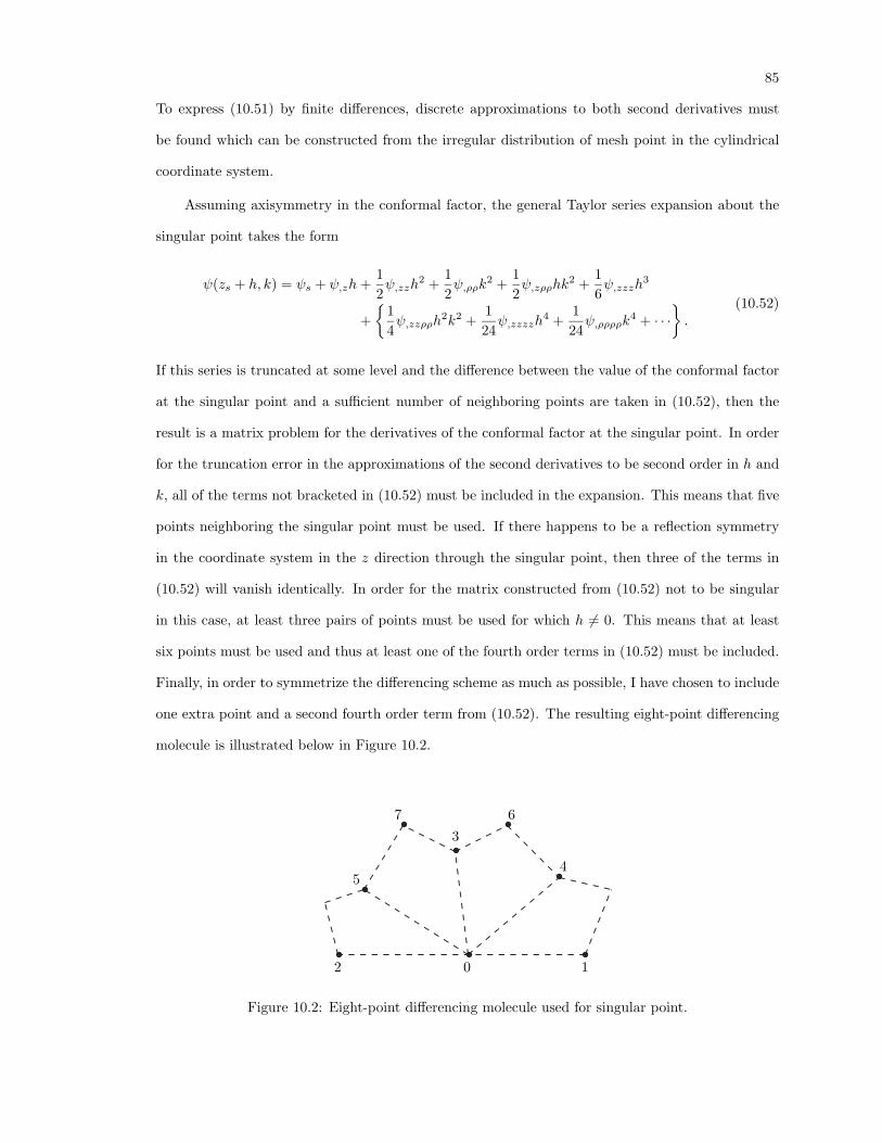
85

To express (10.51) by finite differences, discrete approximations to both second derivatives must

be found which can be constructed from the irregular distribution of mesh point in the cylindrical

coordinate system.

Assuming axisymmetry in the conformal factor, the general Taylor series expansion about the

singular point takes the form

ψ(zs + h, k) = ψs + ψ,zh+12ψ,zzh

2 +12ψ,ρρk

2 +12ψ,zρρhk

2 +16ψ,zzzh

3

+

14ψ,zzρρh

2k2 +124ψ,zzzzh

4 +124ψ,ρρρρk

4 + · · ·.

(10.52)

If this series is truncated at some level and the difference between the value of the conformal factor

at the singular point and a sufficient number of neighboring points are taken in (10.52), then the

result is a matrix problem for the derivatives of the conformal factor at the singular point. In order

for the truncation error in the approximations of the second derivatives to be second order in h and

k, all of the terms not bracketed in (10.52) must be included in the expansion. This means that five

points neighboring the singular point must be used. If there happens to be a reflection symmetry

in the coordinate system in the z direction through the singular point, then three of the terms in

(10.52) will vanish identically. In order for the matrix constructed from (10.52) not to be singular

in this case, at least three pairs of points must be used for which h 6= 0. This means that at least

six points must be used and thus at least one of the fourth order terms in (10.52) must be included.

Finally, in order to symmetrize the differencing scheme as much as possible, I have chosen to include

one extra point and a second fourth order term from (10.52). The resulting eight-point differencing

molecule is illustrated below in Figure 10.2.

0 12

3

45

67

1Figure 10.2: Eight-point differencing molecule used for singular point.

86

Using the labeling in Figure 10.2, the matrix problem for the derivatives becomes

h1 h21 0 0 h3

1 h41 0

h2 h22 0 0 h3

2 h42 0

h3 h23 k2

3 h3k23 h3

3 h43 k4

3

h4 h24 k2

4 h4k24 h3

4 h44 k4

4

h5 h25 k2

5 h5k25 h3

5 h45 k4

5

h6 h26 k2

6 h6k26 h3

6 h46 k4

6

h7 h27 k2

7 h7k27 h3

7 h47 k4

7

ψ,z12ψ,zz12ψ,ρρ12ψ,zρρ16ψ,zzz124ψ,zzzz124ψ,ρρρρ

=

ψ1 − ψ0 −O(h51)

ψ2 − ψ0 −O(h52)

ψ3 − ψ0 −O(h23k

23)

ψ4 − ψ0 −O(h24k

24)

ψ5 − ψ0 −O(h25k

25)

ψ6 − ψ0 −O(h26k

26)

ψ7 − ψ0 −O(h27k

27)

, (10.53)

where

hi ≡ zi − z0 and ki ≡ ρi. (10.54)

Having chosen a discretization for the domain of the problem being solved, all quantities in the

matrix of (10.53) are fixed and the inverse matrix can be computed numerically. If the elements of

the inverse matrix are denoted by M−1i,j , then the differenced form of the Laplacian at the singular

point can be written as

∇2ψ =

7∑i=1

(2M−1

2,i + 4M−13,i

)(ψi − ψ0)

−

7∑i=3

(2M−1

2,i + 4M−13,i

)O(h2

i k2i ). (10.55)

The overall truncation error to this scheme is O(h2 + k2 + hk) and so the rate of decrease in the

error is quadratic as h and k decrease. This does not, however, accurately describe the reduction in

the truncation error as the discretization size in Cadez coordinates is reduced. If the discretization

of the Cadez coordinates is fine enough so that the local expansion of the coordinate transformation

(10.15) is valid, then it is seen that the reduction in the cylindrical discretization length goes as

the square root of the reduction of the Cadez discretization length. This means that the limiting

behavior of the truncation error of (10.55) will be first-order or linear, not quadratic. As in the

case of bispherical coordinates, the presence of this sort of coordinate singularity leads to first-order

behavior for the discretization error.

The difference equations described above for the Hamiltonian constraint in Cadez coordinates

are solved via the Newton-Raphson method for nonlinear systems as described in Chapter 8. As

with the bispherical coordinates, the linearized equations for the iterative correction have been

solved directly by means of the LINPACK routines for factoring (DGBFA) and solving (DGBSL)

general banded matrices. Because of the multiple region nature of the Cadez coordinate system,

the number of bands and the maximum separation of the bands from the diagonal of the matrix

are larger than in the case of bispherical coordinates. The effect of this is that the size of the

matrix which can be solved with these LINPACK routines is substantially less than in the case of

bispherical coordinates. This means that the discretization of the domain cannot be done as finely

87

as is possible with bispherical coordinates and, consequently, the accuracy of the solution will not

be as great. An alternate approach for solving the Cadez coordinate difference equations would be

of great help in this regard. Some work has been done on applying the multigrid approach to this

problem, but with only modest success. It is likely that the multiple region nature of the domain and

difficulties associated with the coordinate singularity are responsible for the less than satisfactory

behavior of the multigrid solver written for this problem. A detailed investigation of the applicability

of the multigrid method to the Cadez coordinate system will be necessary in order to advance this

approach.

Given a solution to the difference equations, the total ADM energy and dipole moment as well

as the minimal surface masses and the physical hole separations can be computed via numerical

integrals. As in the case of bispherical coordinates, care must be taken in numerically integrating

near the singular point. Extrapolative integral formulas have been used unless otherwise stated. In

terms of Cadez coordinates, the total energy is given in dimensionless form by

E

a1=

12

∫ ξs

0

ψρdξ√η2,ρ + η2

,z

∣∣∣∣∣∣(η=η+)

+α

2

∫ π

ξs

ψρdξ√η2,ρ + η2

,z

∣∣∣∣∣∣(η=η−)

+18

ξ=ξs∫ξ=0

η=ηs∫η=η+

(a2

1AijAij)

ψ7

ρdηdξ

η2,ρ + η2

,z

+18

ξ=π∫ξ=ξs

η=ηs∫η=η−

(a2

1AijAij)

ψ7

ρdηdξ

η2,ρ + η2

,z

+18

ξ=π∫ξ=0

η=∞∫η=ηs

(a2

1AijAij)

ψ7

ρdηdξ

η2,ρ + η2

,z

.

(10.56)

The z component of the dipole moment is given in dimensionless form by

dza2

1

=

ξs∫0

zψ2 +η,z(1− ψ)√η2,ρ + η2

,z

ρdξ√η2,ρ + η2

,z

∣∣∣∣∣∣(η=η+)

+18

ξ=ξs∫ξ=0

η=ηs∫η=η+

(a2

1AijAij)

ψ7

zρdηdξ

η2,ρ + η2

,z

+

π∫ξs

αzψ2 +η,z(1− ψ)√η2,ρ + η2

,z

ρdξ√η2,ρ + η2

,z

∣∣∣∣∣∣(η=η−)

+18

ξ=π∫ξ=ξs

η=ηs∫η=η−

(a2

1AijAij)

ψ7

zρdηdξ

η2,ρ + η2

,z

+18

ξ=π∫ξ=0

η=∞∫η=ηs

(a2

1AijAij)

ψ7

zρdηdξ

η2,ρ + η2

,z

.

(10.57)

The areas of the minimal surfaces are given in dimensionless form by

A+MS

a21

= 2π∫ ξs

0

ψ4ρdξ√η2,ρ + η2

,z

∣∣∣∣∣∣(η=η+)

(10.58a)

88

andA−MS

a21

= 2π∫ π

ξs

ψ4ρdξ√η2,ρ + η2

,z

∣∣∣∣∣∣(η=η−)

. (10.58b)

Finally, the proper separation of the two holes is given in dimensionless form by

L

a1= −

∫ ηs

η+

ψ2dη

η,z

∣∣∣∣(ξ=ξs)

+∫ ηs

η−

ψ2dη

η,z

∣∣∣∣(ξ=ξs)

. (10.59)

The numerical approximation of (10.59) tends to be a poor approximation because of the relative

sparseness of mesh points between the two holes. The accuracy of the approximation can be greatly

increased by replacing (10.59) with an integral over three separate regions. (10.59) consists of an

integral along the z-axis between the holes in Regions 1 and 2. The third integral is taken to be

from one mesh point to the left of the singular point in Region 2 to one mesh point to the right of

the singular point in Region 1. The two integrals in (10.59) are adjusted so as not to include this

section. The value of the conformal factor in the intermediate section can be approximated by a

quadratic polynomial fit to the three values of the conformal factor at the singular point and its

nearest neighbors. This interpolated conformal factor can then be integrated analytically in cylin-

drical coordinates giving a more accurate result than can be achieved by a standard, extrapolative

numerical integral. Using the notation of Figure 10.2, the contribution of this section to the total

proper separation is given by

L

a1= ψ2

1

(z1 − z2)6(z1 − z0)

(2z1 − 3z0 + z2) + ψ20

(z1 − z2)3

6(z1 − z0)(z0 − z2)

− ψ22

(z1 − z2)6(z0 − z2)

(z1 − 3z0 + 2z2).(10.60)

Because the numerical integrals for the total energy and dipole moment cannot extend past the

outer boundary of the computational domain, the integrals (10.56) and (10.57) necessarily incorpo-

rate error beyond that introduced by the numerical approximations. An understanding of the nature

of this error as well as a first-order correction to the numerical result can be obtained by examining

the asymptotic forms of the integrands of (10.56) and (10.57) and estimating the contribution from

the integral over the domain exterior to the outer boundary.

For the case of two holes with axisymmetric linear and angular momenta, we find (see (7.22))

that at large radius the square of the extrinsic curvature takes the dimensionless form

a21AijA

ij ≈ 92r4

(P1/a1 + P2/a1)2 (1 + 2cos2θ). (10.61)

(Note that r is dimensionless.) Similarly, from (7.26) we find for the conformal factor

ψ ≈ 1 +E/a1

2r+dz/a

21

2r2cos θ − 9

32(P1/a1 + P2/a1)2

r2(1− 2cos2θ). (10.62)

89

Using (10.61) and (10.62), the leading order contributions to the total energy and dipole moment,

resulting from the integral over the region exterior to a sphere of radius rb, are

∆E/a1 ≈158

(P1/a1 + P2/a1)2

rb− 105

32(P1/a1 + P2/a1)2

r2b

E

a1(10.63)

and

∆dz/a21 ≈ −

231160

(P1/a1 + P2/a1)2

r2b

dza2

1

. (10.64)

If results of the numerical integration over the finite domain for the total energy and dipole

moment are denoted respectively by EN/a1 and dN/a21, then first-order corrected values are given

by

E

a1≈EN/a1 + 15

8(P1/a1+P2/a1)2

rb

1 + 10532

(P1/a1+P2/a1)2

r2b

(10.65)

anddza2

1

≈ dN/a21

1 + 231160

(P1/a1+P2/a1)2

r2b

. (10.66)

It is easy to see from (10.65) and (10.66) that configurations with a non-vanishing net linear mo-

mentum will suffer the worst errors from the approximation of a finite computational domain and

this error can, for the most part, be compensated for by the use of (10.65) and (10.66).

Appendix D contains the results from computational solutions covering a large set of configu-

rations and grid resolutions. Each of these computations, performed in Cadez coordinates, can be

directly compared to an identical computation performed in bispherical coordinates and tabulated

in Appendix C. Because of the behavior of the discretization between the holes, configurations with

small β require very fine discretizations in Region 3 in order to have a moderate discretization in

Regions 1 and 2. The end result of this is that with the current solution method, only very coarse

grids can be used when β is small. Consequently, the accuracy of the solution is rather poor in these

cases. For the case of β = 3, the errors in the total energy where on the order of 20% and the errors

in the separation were roughly 30%. This is not at all surprising considering that only 12 discrete

zones were present between the holes while in bispherical coordinates, 160 where used in the finest

discretization. On the other hand, when β reached 6, the errors were down to less than 1% when

there was no net momentum and to 5% when there was. This is an encouraging level of error for

the cases with no net momenta. The higher error in the cases with a net momentum indicate that

the outer boundary, placed at radius of roughly 200a1, was somewhat too close.

These preliminary solutions using Cadez coordinates, while less accurate than those obtained

with bispherical coordinates, show that there is no fundamental problem with the use of Cadez

90

coordinates for work on the two-hole initial-value and evolution problems. The differencing scheme

discussed above appears to work adequately. The remaining difficuly lies in finding computational

routines for solving the large, poorly banded matrices which result from the differencing scheme.

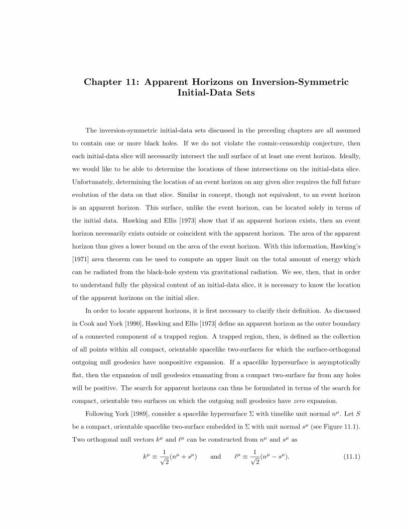
Chapter 11: Apparent Horizons on Inversion-SymmetricInitial-Data Sets

The inversion-symmetric initial-data sets discussed in the preceding chapters are all assumed

to contain one or more black holes. If we do not violate the cosmic-censorship conjecture, then

each initial-data slice will necessarily intersect the null surface of at least one event horizon. Ideally,

we would like to be able to determine the locations of these intersections on the initial-data slice.

Unfortunately, determining the location of an event horizon on any given slice requires the full future

evolution of the data on that slice. Similar in concept, though not equivalent, to an event horizon

is an apparent horizon. This surface, unlike the event horizon, can be located solely in terms of

the initial data. Hawking and Ellis [1973] show that if an apparent horizon exists, then an event

horizon necessarily exists outside or coincident with the apparent horizon. The area of the apparent

horizon thus gives a lower bound on the area of the event horizon. With this information, Hawking’s

[1971] area theorem can be used to compute an upper limit on the total amount of energy which

can be radiated from the black-hole system via gravitational radiation. We see, then, that in order

to understand fully the physical content of an initial-data slice, it is necessary to know the location

of the apparent horizons on the initial slice.

In order to locate apparent horizons, it is first necessary to clarify their definition. As discussed

in Cook and York [1990], Hawking and Ellis [1973] define an apparent horizon as the outer boundary

of a connected component of a trapped region. A trapped region, then, is defined as the collection

of all points within all compact, orientable spacelike two-surfaces for which the surface-orthogonal

outgoing null geodesics have nonpositive expansion. If a spacelike hypersurface is asymptotically

flat, then the expansion of null geodesics emanating from a compact two-surface far from any holes

will be positive. The search for apparent horizons can thus be formulated in terms of the search for

compact, orientable two surfaces on which the outgoing null geodesics have zero expansion.

Following York [1989], consider a spacelike hypersurface Σ with timelike unit normal nµ. Let S

be a compact, orientable spacelike two-surface embedded in Σ with unit normal sµ (see Figure 11.1).

Two orthogonal null vectors kµ and `µ can be constructed from nµ and sµ as

kµ ≡ 1√2

(nµ + sµ) and `µ ≡ 1√2

(nµ − sµ). (11.1)

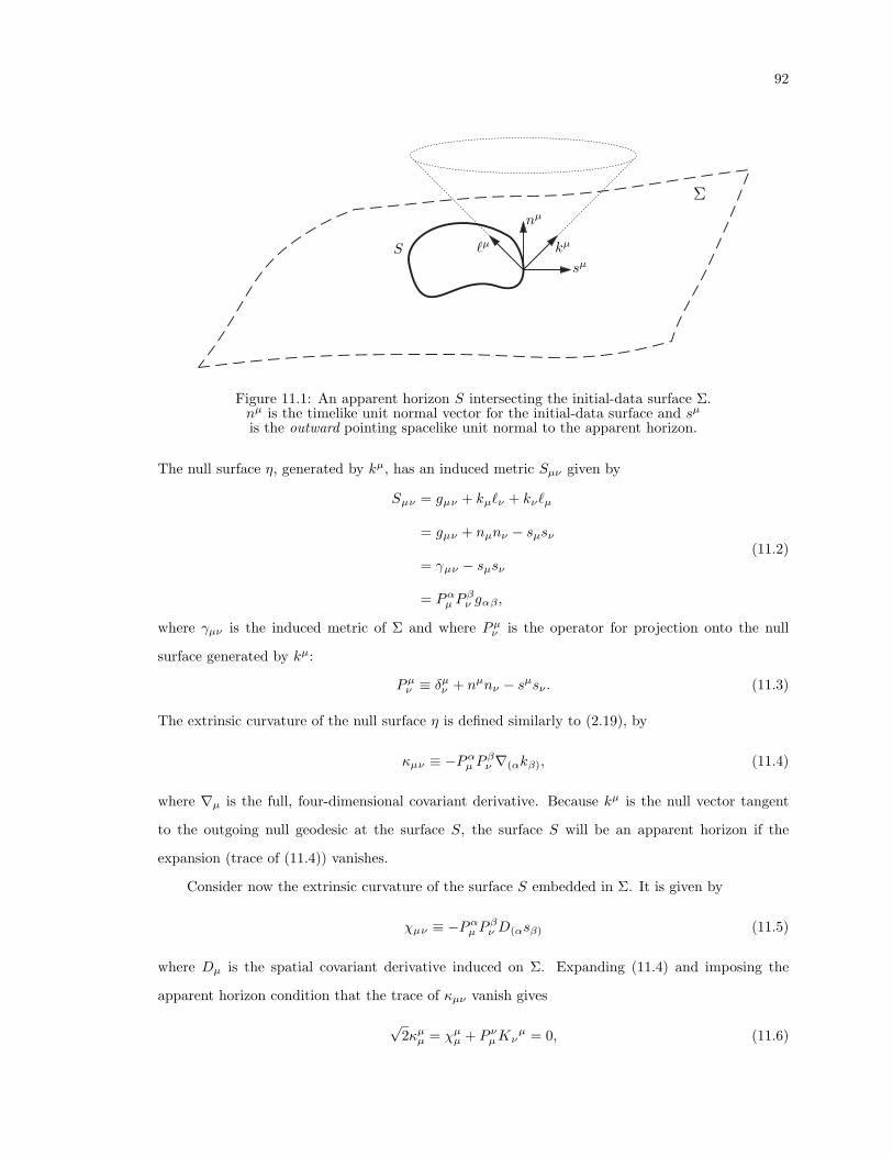
92

S

Σ

sµ

nµ

`µ kµ

1Figure 11.1: An apparent horizon S intersecting the initial-data surface Σ.nµ is the timelike unit normal vector for the initial-data surface and sµ

is the outward pointing spacelike unit normal to the apparent horizon.

The null surface η, generated by kµ, has an induced metric Sµν given by

Sµν = gµν + kµ`ν + kν`µ

= gµν + nµnν − sµsν

= γµν − sµsν

= Pαµ Pβν gαβ ,

(11.2)

where γµν is the induced metric of Σ and where Pµν is the operator for projection onto the null

surface generated by kµ:

Pµν ≡ δµν + nµnν − sµsν . (11.3)

The extrinsic curvature of the null surface η is defined similarly to (2.19), by

κµν ≡ −Pαµ P βν ∇(αkβ), (11.4)

where ∇µ is the full, four-dimensional covariant derivative. Because kµ is the null vector tangent

to the outgoing null geodesic at the surface S, the surface S will be an apparent horizon if the

expansion (trace of (11.4)) vanishes.

Consider now the extrinsic curvature of the surface S embedded in Σ. It is given by

χµν ≡ −Pαµ P βν D(αsβ) (11.5)

where Dµ is the spatial covariant derivative induced on Σ. Expanding (11.4) and imposing the

apparent horizon condition that the trace of κµν vanish gives

√2κµµ = χµµ + P νµKν

µ = 0, (11.6)

93

where Kµν is the extrinsic curvature of Σ embedded in the full space-time. This can be simplified

to

Disi −K +Kijs

isj = 0, (11.7a)

or in terms of (3.8),

Disi − 2

3K +Aijs

isj = 0. (11.7b)

Equation (11.7), thus, represents a necessary condition that si be the outward-pointing unit-normal

to an apparent horizon. If the surface to which si is normal is the outer-most such surface, then

that surface is an apparent horizon. Equation (11.7b) can be expressed in terms of the conformal

background space and the background quantities defined on it. For a unit normal vector, the natural

conformal weighting is given by

si = ψ−2si, (11.8)

where si is the background unit-normal vector. Using the conformal weightings for the metric and

extrinsic curvature from Chapter 3, (11.7b) becomes

Disi + 4siDi lnψ − 2

3ψ2K + ψ−4Aij s

isj = 0. (11.9)

Equation (11.9) is a single equation for a three-dimensional vector and so it seems at first that it

cannot uniquely determine si. Recalling that si must be a unit vector removes one degree of freedom

from si and the fact that the surface of the apparent horizon must be a closed two-surface removes

a second. Together, these conditions demand that

si = λDiτ where λ =[(Diτ)(Diτ)

]−1/2, (11.10)

and where τ is a scalar function whose level surface τ = τ0 defines the position of the apparent

horizon. Using (11.10) in (11.9) gives the final form for the apparent-horizon equation

λ∇2τ + (Diλ)(Diτ) + 4λ(Di lnψ)(Diτ)− 2

3ψ2K + ψ−4λ2Aij(Diτ)(Djτ) = 0. (11.11)

The apparent-horizon equation is thus in the form of a highly nonlinear partial differential equation

for the scalar function τ which can be solved numerically by a variety of means.

If the manifold on which the initial data is specified is inversion-symmetric, as is the case for

the initial data described in earlier chapters, then the apparent horizon must be inversion-symmetric

as well. The unit normal to the surface of the apparent horizon, as with all vector fields defined on

the manifold, must satisfy isometry condition (4.36), so

si(x) = ±(J−1α )jisj(Jα(x)). (11.12)

94

In terms of the conformal background fields, this becomes

si(x) = ±(aαrα

)2

(J−1α )jisj(Jα(x)). (11.13)

To prove that apparent horizons on initial-data slices which contain inversion-symmetric initial data

are themselves inversion-symmetric, let us assume that si(x) is a solution of the apparent-horizon

equation (11.9), where x belongs to the set of points which satisfies τ(x) = τ0. The inversion-

symmetric counterpart must then be the vector field si(x) defined by

si(x) = ±(aαrα

)2

(J−1α )jisj(Jα(x)). (11.14)

In terms of Cartesian coordinates and using (4.40) and (4.49)–(4.54), direct calculation shows that

Disi(x) = ±

(r′αaα

)2 [D′is

i(x′)− 4r′αn′αi s

i(x′)], (11.15)

si(x)Di lnψ(x) = ±(r′αaα

)2

si(x′)[D′i lnψ(x′) +

1r′αn′αi

], (11.16)

ψ−2(x)K(x) = ±(r′αaα

)2

ψ−2(x′)K(x′), (11.17)

and

ψ−4(x)Aij(x)si(x)sj(x) = ±(r′αaα

)2 [ψ−4(x′)Aij(x′)si(x′)sj(x′)

]. (11.18)

Thus, we find that the apparent-horizon equation for si(x) becomes

Disi(x) + 4si(x)Di lnψ(x)− 2

3ψ2(x)K(x) + ψ−4(x)Aij(x)si(x)sj(x)

= ±(r′αaα

)2[D′is

i(x′) + 4si(x′)D′i lnψ(x′)− 23ψ2(x′)K(x′)

+ψ−4(x′)Aij(x′)si(x′)sj(x′)].

(11.19)

Since the right-hand side of (11.19) satisfies the apparent-horizon equation for x′ such that τ(x′) = τ0,

we find that si(x) satisfies the apparent-horizon equation for x such that τ(Jα(x)) = τ0.

Many methods can be used to locate apparent horizons by solving the apparent-horizon equation

(11.11). For the case of two black holes on a time-symmetric slice, several authors (Cadez [1974]

and Bishop [1982] and [1984]) have searched for apparent horizons (minimal surfaces in the time-

symmetric case) by means of “shooting” methods. Unfortunately, this method is applicable only

to axisymmetric initial-data sets since it is an inherently one-dimensional method. Nakamura et

al. [1984] and [1985] have developed and tested a method for locating apparent horizons based on

an expansion in spherical harmonics. This approach is applicable to full, three-dimensional initial-

data sets. An alternative approach which I have developed (Cook and York [1990]) is to solve

95

(11.11) directly as a boundary value problem. This approach is also applicable to three-dimensional

initial-data sets.

I have applied this approach to the problem of locating the apparent horizons in the one-hole

initial-data sets discussed in Chapter 8. In the next chapter, I will describe the method and the

solutions found. In the future, it will be essential to locate the apparent horizons in the two-hole

initial-data sets. This work has not yet been undertaken, although it is planned for the near future.

Chapter 12: Apparent Horizons for a Single Black Holewith Linear or Angular Momentum

Given the initial data for a single black hole with non-zero linear or angular momentum as

described in Chapter 8, the apparent-horizon equation (11.11) can be solved to locate any apparent

horizons on the initial-data slice. Because part of the initial data is only known numerically, it will

be necessary to solve (11.11) numerically. As described in Chapter 11, this will be accomplished by

posing the apparent-horizon equation as a boundary value problem.

As stated in Chapter 11, the location of apparent horizons is determined by solving (11.11) for

the scalar function τ of which the level surface τ = τ0 is the apparent horizon. For this approach to

work, the functional form for τ must be chosen carefully. The apparent horizons for the case of a

single hole are expected to be located near to the minimal surface. Using the logarithmically scaled

dimensionless radial coordinates (8.1) from Chapter 8, an appropriate choice for τ is

τ(x, θ, φ) = x− h(θ, φ). (12.1)

Choosing the level surface τ = 0 to locate the apparent horizon then means that the radius of the

apparent horizon is given parametrically by

x = h(θ, φ). (12.2)

From (11.10) we find that

λ = aeh(θ,φ)(1 + h2,θ + h2

,φ/sin2θ)−1/2

(12.3)

and

si =1

aeh(θ,φ)√

1 + h2,θ + h2

,φ/sin2θ

[ 1 −h,θ −h,φ/sin2θ ] . (12.4)

Note that any occurrence of the coordinate x must be evaluated at x = h(θ, φ). From (12.4) it is

seen that si is indeed an outward pointing unit normal from the point of view of an observer on the

top sheet (x > 0).

Since the initial-data slices constructed in Chapter 8 for a single hole are inversion symmetric,

any solution of the apparent-horizon equation must have an inversion-symmetric counterpart. To

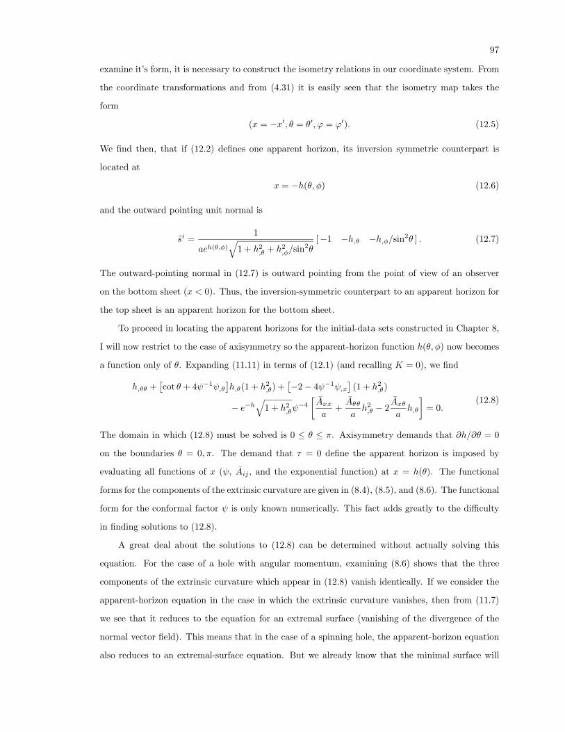
97

examine it’s form, it is necessary to construct the isometry relations in our coordinate system. From

the coordinate transformations and from (4.31) it is easily seen that the isometry map takes the

form

(x = −x′, θ = θ′, ϕ = ϕ′). (12.5)

We find then, that if (12.2) defines one apparent horizon, its inversion symmetric counterpart is

located at

x = −h(θ, φ) (12.6)

and the outward pointing unit normal is

si =1

aeh(θ,φ)√

1 + h2,θ + h2

,φ/sin2θ

[−1 −h,θ −h,φ/sin2θ ] . (12.7)

The outward-pointing normal in (12.7) is outward pointing from the point of view of an observer

on the bottom sheet (x < 0). Thus, the inversion-symmetric counterpart to an apparent horizon for

the top sheet is an apparent horizon for the bottom sheet.

To proceed in locating the apparent horizons for the initial-data sets constructed in Chapter 8,

I will now restrict to the case of axisymmetry so the apparent-horizon function h(θ, φ) now becomes

a function only of θ. Expanding (11.11) in terms of (12.1) (and recalling K = 0), we find

h,θθ +[cot θ + 4ψ−1ψ,θ

]h,θ(1 + h2

,θ) +[−2− 4ψ−1ψ,x

](1 + h2

,θ)

− e−h√

1 + h2,θψ−4

[Axxa

+Aθθah2,θ − 2

Axθah,θ

]= 0.

(12.8)

The domain in which (12.8) must be solved is 0 ≤ θ ≤ π. Axisymmetry demands that ∂h/∂θ = 0

on the boundaries θ = 0, π. The demand that τ = 0 define the apparent horizon is imposed by

evaluating all functions of x (ψ, Aij , and the exponential function) at x = h(θ). The functional

forms for the components of the extrinsic curvature are given in (8.4), (8.5), and (8.6). The functional

form for the conformal factor ψ is only known numerically. This fact adds greatly to the difficulty

in finding solutions to (12.8).

A great deal about the solutions to (12.8) can be determined without actually solving this

equation. For the case of a hole with angular momentum, examining (8.6) shows that the three

components of the extrinsic curvature which appear in (12.8) vanish identically. If we consider the

apparent-horizon equation in the case in which the extrinsic curvature vanishes, then from (11.7)

we see that it reduces to the equation for an extremal surface (vanishing of the divergence of the

normal vector field). This means that in the case of a spinning hole, the apparent-horizon equation

also reduces to an extremal-surface equation. But we already know that the minimal surface will

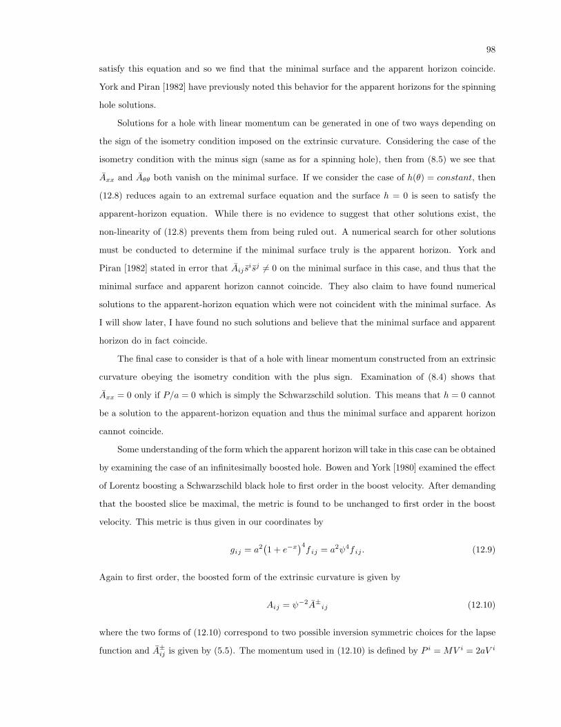
98

satisfy this equation and so we find that the minimal surface and the apparent horizon coincide.

York and Piran [1982] have previously noted this behavior for the apparent horizons for the spinning

hole solutions.

Solutions for a hole with linear momentum can be generated in one of two ways depending on

the sign of the isometry condition imposed on the extrinsic curvature. Considering the case of the

isometry condition with the minus sign (same as for a spinning hole), then from (8.5) we see that

Axx and Aθθ both vanish on the minimal surface. If we consider the case of h(θ) = constant, then

(12.8) reduces again to an extremal surface equation and the surface h = 0 is seen to satisfy the

apparent-horizon equation. While there is no evidence to suggest that other solutions exist, the

non-linearity of (12.8) prevents them from being ruled out. A numerical search for other solutions

must be conducted to determine if the minimal surface truly is the apparent horizon. York and

Piran [1982] stated in error that Aij sisj 6= 0 on the minimal surface in this case, and thus that the

minimal surface and apparent horizon cannot coincide. They also claim to have found numerical

solutions to the apparent-horizon equation which were not coincident with the minimal surface. As

I will show later, I have found no such solutions and believe that the minimal surface and apparent

horizon do in fact coincide.

The final case to consider is that of a hole with linear momentum constructed from an extrinsic

curvature obeying the isometry condition with the plus sign. Examination of (8.4) shows that

Axx = 0 only if P/a = 0 which is simply the Schwarzschild solution. This means that h = 0 cannot

be a solution to the apparent-horizon equation and thus the minimal surface and apparent horizon

cannot coincide.

Some understanding of the form which the apparent horizon will take in this case can be obtained

by examining the case of an infinitesimally boosted hole. Bowen and York [1980] examined the effect

of Lorentz boosting a Schwarzschild black hole to first order in the boost velocity. After demanding

that the boosted slice be maximal, the metric is found to be unchanged to first order in the boost

velocity. This metric is thus given in our coordinates by

gij = a2(1 + e−x

)4f ij = a2ψ4f ij . (12.9)

Again to first order, the boosted form of the extrinsic curvature is given by

Aij = ψ−2A±ij (12.10)

where the two forms of (12.10) correspond to two possible inversion symmetric choices for the lapse

function and A±ij is given by (5.5). The momentum used in (12.10) is defined by P i = MV i = 2aV i

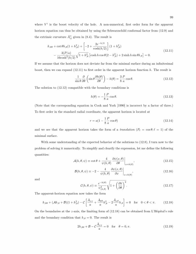
99

where V i is the boost velocity of the hole. A non-numerical, first order form for the apparent

horizon equation can thus be obtained by using the Schwarzschild conformal factor from (12.9) and

the extrinsic curvature A+ij given in (8.4). The result is

h,θθ + cot θh,θ(1 + h2,θ) +

[−2 +

2e−h/2

cosh(h/2)

](1 + h2

,θ)

− 3(P/a)16cosh2(h/2)

√1 + h2

,θ

[coshh cos θ(2− h2

,θ) + 2 sinhh sin θh,θ]

= 0.(12.11)

If we assume that the horizon does not deviate far from the minimal surface during an infinitesimal

boost, then we can expand (12.11) to first order in the apparent horizon function h. The result is

1sin θ

∂

∂θ

(sin θ

∂h(θ)∂θ

)− h(θ) =

38P

acos θ. (12.12)

The solution to (12.12) compatible with the boundary conditions is

h(θ) = −18P

acos θ. (12.13)

(Note that the corresponding equation in Cook and York [1990] is incorrect by a factor of three.)

To first order in the standard radial coordinate, the apparent horizon is located at

r = a(1− 18P

acos θ) (12.14)

and we see that the apparent horizon takes the form of a translation (P` = cos θ; ` = 1) of the

minimal surface.

With some understanding of the expected behavior of the solutions to (12.8), I turn now to the

problem of solving it numerically. To simplify and clearify the expression, let me define the following

quantities:

A(h, θ, ψ) ≡ cot θ +4

ψ(h, θ)∂ψ(x, θ)∂θ

∣∣∣∣x=h(θ)

, (12.15)

B(h, θ, ψ) ≡ −2− 4ψ(h, θ)

∂ψ(x, θ)∂x

∣∣∣∣x=h(θ)

, (12.16)

and

C(h, θ, ψ) ≡ e−h(θ)

ψ4(h,θ)

√1 +

(∂h

∂θ

)2

. (12.17)

The apparent-horizon equation now takes the form

h,θθ + (Ah,θ + B)(1 + h2,θ)− C

[Axxa

+Aθθah2,θ − 2

Axθah,θ

]= 0 for 0 < θ < π. (12.18)

On the boundaries at the z-axis, the limiting form of (12.18) can be obtained from L’Hopital’s rule

and the boundary condition that h,θ = 0. The result is

2h,θθ + B − C Axxa

= 0 for θ = 0, π. (12.19)

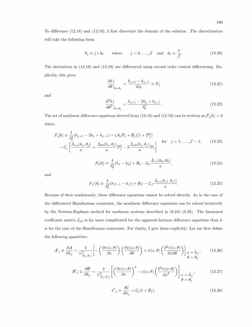
100

To difference (12.18) and (12.19), I first discretize the domain of the solution. The discretization

will take the following form:

θj ≡ j ∗ δθ where j = 0, . . . ,J and δθ ≡π

J. (12.20)

The derivatives in (12.18) and (12.19) are differenced using second order central differencing. Ex-

plicitly, this gives∂h

∂θ

∣∣∣∣θ=θj

=hj+1 − hj−1

2δθ≡ Dj (12.21)

and∂2h

∂θ2

∣∣∣∣θ=θj

=hj+1 − 2hj + hj−1

δ2θ

. (12.22)

The set of nonlinear difference equations derived from (12.18) and (12.19) can be written as Fj [h] = 0

where

Fj [h] ≡ 1δ2θ

(hj+1 − 2hj + hj−1) + (AjDj + Bj)(1 +D2j )

− Cj[Axx(hj , θj)

a+Aθθ(hj , θj)

aD2j − 2

Axθ(hj , θj)a

Dj] for j = 1, . . . ,J − 1, (12.23)

F0[h] ≡ 4δ2θ

(h1 − h0) + B0 − C0Axx(h0, θ0)

a, (12.24)

and

FJ [h] ≡ 4δ2θ

(hJ−1 − hJ ) + BJ − CJAxx(hJ , θJ )

a. (12.25)

Because of their nonlinearity, these difference equations cannot be solved directly. As in the case of

the differenced Hamiltonian constraint, the nonlinear difference equations can be solved iteratively

by the Newton-Raphson method for nonlinear systems described in (8.24)–(8.28). The linearized

coefficient matrix Lab is far more complicated for the apparent-horizon difference equations than it

is for the case of the Hamiltonian constraint. For clarity, I give them explicitly. Let me first define

the following quantities:

A′j ≡∂A∂hj

=4

ψ2(hj ,θj)

[−(∂ψ(x, θ)∂x

)(∂ψ(x, θ)∂θ

)+ ψ(x, θ)

(∂2ψ(x, θ)∂x∂θ

)]x = hjθ = θj

, (12.26)

B′j ≡∂B∂hj

=4

ψ2(hj ,θj)

[(∂ψ(x, θ)∂x

)2

− ψ(x, θ)(∂2ψ(x, θ)∂x2

)]x = hjθ = θj

, (12.27)

C′j ≡∂C∂hj

= Cj(1 + Bj), (12.28)

101

and

A′`m ≡∂A`m∂x

∣∣∣∣x = hjθ = θj

(12.29)

where h is the current estimate for the apparent horizon function. The non-zero elements of the

linearized coefficient matrix are

Lj,j [h] = − 2δ2θ

+ (A′jDj + B′j)(1 +D2j )− Cj

[A′xxa

+A′θθaD2j − 2

A′xθaDj]

+C′j

[Axx(hj , θj)

a+Aθθ(hj , θj)

aD2j − 2

Axθ(hj , θj)a

Dj

]for j = 1, . . . ,J − 1,

(12.30)

Lj,j [h] = − 4δ2θ

+ B′j − Cj

[A′xxa

+ (1 + Bj)Axx(hj , θj)

a

]for j = 0,J , (12.31)

Lj,j±1[h] =1δ2θ

±

Aj

1 +D2j

2δθ+ (AjDj + Bj)

Djδθ− Cj

(1 +D2j )δθ

[Axx(hj , θj)

a

Dj2

+Aθθ(hj , θj)

a

(3D2j + 2)Dj

2− Axθ(hj , θj)

a(2D2

j + 1)

]for j = 1, . . . ,J − 1,

(12.32)

and

L0,1[h] =4δ2θ

and LJ ,J−1[h] =4δ2θ

. (12.33)

Inspection of the linearized coefficient matrix shows it to be tridiagonal and so it can be easily

inverted directly by a tridiagonal matrix solver.

There is one difficult point in evaluating the intermediate functions (12.15), (12.16), and (12.17)

and their derivatives (12.26), (12.27), and (12.28). These functions depend upon the conformal factor

ψ and its derivatives which are known only numerically on a discrete mesh. From the form of the

discretization of the conformal factor ψ (8.13) and (8.14), and from the form of the discretization

of the apparent-horizon function h (12.20), it is apparent that the discretization of h can be chosen

to match that of the conformal factor. This means that the conformal factor and its derivatives

need only be evaluated along lines of constant θ on which values of the conformal factor are known

numerically. Unfortunately, the radial position at which the conformal factor must be evaluated is

not discretized and will, in general, not occur at a location at which the conformal factor is known.

The evaluation of the conformal factor will thus require interpolation in the radial direction.

The main criterion for choosing an interpolation algorithm is the requirement that the conformal

factor and its derivatives be continuous functions. From (12.15), (12.16), (12.26), and (12.27) we

find that the highest order radial derivative needed is a second derivative. Interpolation by cubic

102

splines (cf. Press et al. [1988]) has sufficient smoothness so that its second derivatives are continuous

(though not smooth) and I have chosen to use this approach for the radial interpolation. The radial

derivatives can be evaluated by analytically differentiating the cubic spline interpolation formula.

Angular derivatives of the conformal factor can be evaluated using second order centered difference

approximations.

The possibility of the introduction of high frequency noise must always be considered when

numerical data is differentiated. The use of cubic splines and the analytic differentiation of these,

rather than the numerical data itself, helps to eliminate possible high frequency noise in radial

derivatives. Another step which can be taken to eliminate such effects is to factor out the gross

variations in the numerical data into an analytic prefactor (Piran [1988]). For the case of the

one-hole initial-data sets, such a factorization can take the form

ψ(x, θ) = f(x)N (x, θ) where f(x) ≡ 1 +12E

ae−x. (12.34)

The prefactor f(x) is simply the conformal factor for a time-symmetric solution with scaled total

energy E/a. By factoring this out of the numerical solution, the resulting numerical data N (x, θ)

will be a more slowly varying function of x and the interpolation of this data will be less prone to

high frequency noise. No extra effort was needed to reduce noise for the numerical derivatives in the

θ direction since the conformal factor is already a slowly varying function in this direction.

One final point needs to be explained regarding the evaluation of the conformal factor and

its derivatives. The Hamiltonian constraint was solved over the finite range of 0 ≤ x ≤ xf and

0 ≤ θ ≤ π/2. The range over which the apparent-horizon equation must be solved is 0 ≤ θ ≤ π.

The extension of the numerical data to cover this region is easily achieved since

ψ(x, θ) = ψ(x, π − θ) for π/2 ≤ θ ≤ π. (12.35)

It will also be necessary to evaluate the conformal factor for x < 0. Values in this range can be

obtained from the isometry condition (4.53). Written in terms of the logarithmically scaled radial

coordinates we find

ψ(x, θ) = e|x|ψ(|x| , θ) for x < 0. (12.36)

Finally, if the conformal factor is needed in the region outside the outer boundary of the domain

x > xf , this can be approximated by (7.13) (same as f(x) from (12.34)) which is the basis for the

outer boundary condition imposed at xf .

A computer code based on the method described above was constructed to solve for the

apparent-horizon function h(θ) and was used to locate the apparent horizons on all of the initial-data

103

sets described in Chapter 8. In addition to computing the location of the apparent horizon, the code

also computed the area and mass (via (8.33)) of the apparent horizon. The integral for the area of

the apparent horizon is obtained by starting with the physical metric for the initial-data slice

ds2 = a2e2xψ4(dx2 + dθ2 + sin2θdφ2) (12.37)

and using the parametrically defined location of the apparent horizon (12.2) to reduce (12.37) to the

induced metric on the apparent horizon

ds2 = a2e2h(θ)ψ4(h(θ),θ)((1 + h2

,θ)dθ2 + sin2θdφ2). (12.38)

From (12.38), the integral for the physical area of the apparent horizon is given in dimensionless

form by

AAH

a2= 2π

∫ π

0

ψ4(h(θ),θ)e

2h(θ)√

1 + h2,θ sin θdθ. (12.39)

For the case of a hole with linear or angular momentum generated from an extrinsic curvature

obeying the isometry condition with the minus sign, no solutions except the one coincident with

the minimal surface were found. Other solutions were sought by varying the initial guess for the

location of the apparent horizon. Convergence to the minimal surface solution was always direct,

with no indication of other possible solutions.

For the case of a hole with linear momentum generated from an extrinsic curvature obeying the

isometry condition with the plus sign, a single solution, not coincident with the minimal surface,

was found for each initial-data set. The apparent-horizon function for the case of P/a = 10 is shown

in Figure 12.1. The general sinusoidal shape is inherent for all values of the momentum. In fact, to

within the truncation error of the problem, the solution is given by

h(θ) = H(P/a) cos θ (12.40)

where the amplitude H is a function of the scaled momentum only. Table 12.1 lists the masses for

the minimal surface MMS and the apparent horizon MAH along with the value of the amplitude H

and its standard deviation σ resulting from a least-squares fit of the numerical data for h(θ) to the

functional form (12.40).

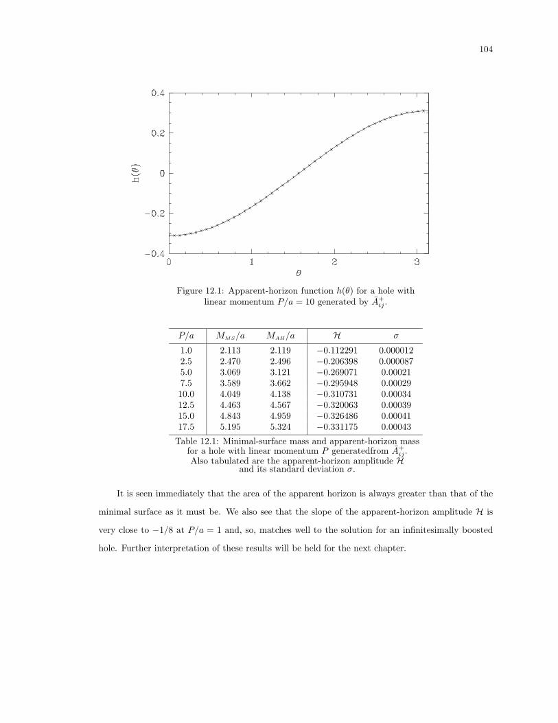
104

1Figure 12.1: Apparent-horizon function h(θ) for a hole withlinear momentum P/a = 10 generated by A+

ij .

P/a MMS/a MAH/a H σ

1.0 2.113 2.119 −0.112291 0.0000122.5 2.470 2.496 −0.206398 0.0000875.0 3.069 3.121 −0.269071 0.000217.5 3.589 3.662 −0.295948 0.0002910.0 4.049 4.138 −0.310731 0.0003412.5 4.463 4.567 −0.320063 0.0003915.0 4.843 4.959 −0.326486 0.0004117.5 5.195 5.324 −0.331175 0.00043

Table 12.1: Minimal-surface mass and apparent-horizon massfor a hole with linear momentum P generatedfrom A+

ij .Also tabulated are the apparent-horizon amplitude H

and its standard deviation σ.

It is seen immediately that the area of the apparent horizon is always greater than that of the

minimal surface as it must be. We also see that the slope of the apparent-horizon amplitude H is

very close to −1/8 at P/a = 1 and, so, matches well to the solution for an infinitesimally boosted

hole. Further interpretation of these results will be held for the next chapter.

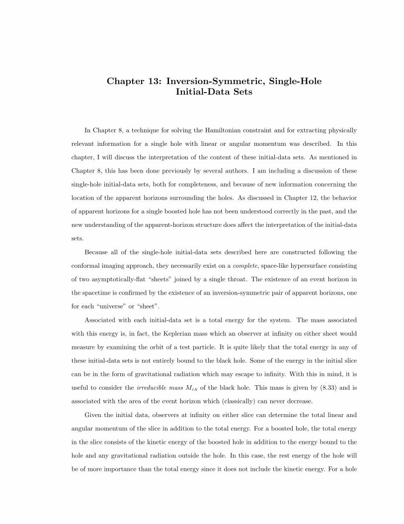
Chapter 13: Inversion-Symmetric, Single-HoleInitial-Data Sets

In Chapter 8, a technique for solving the Hamiltonian constraint and for extracting physically

relevant information for a single hole with linear or angular momentum was described. In this

chapter, I will discuss the interpretation of the content of these initial-data sets. As mentioned in

Chapter 8, this has been done previously by several authors. I am including a discussion of these

single-hole initial-data sets, both for completeness, and because of new information concerning the

location of the apparent horizons surrounding the holes. As discussed in Chapter 12, the behavior

of apparent horizons for a single boosted hole has not been understood correctly in the past, and the

new understanding of the apparent-horizon structure does affect the interpretation of the initial-data

sets.

Because all of the single-hole initial-data sets described here are constructed following the

conformal imaging approach, they necessarily exist on a complete, space-like hypersurface consisting

of two asymptotically-flat “sheets” joined by a single throat. The existence of an event horizon in

the spacetime is confirmed by the existence of an inversion-symmetric pair of apparent horizons, one

for each “universe” or “sheet”.

Associated with each initial-data set is a total energy for the system. The mass associated

with this energy is, in fact, the Keplerian mass which an observer at infinity on either sheet would

measure by examining the orbit of a test particle. It is quite likely that the total energy in any of

these initial-data sets is not entirely bound to the black hole. Some of the energy in the initial slice

can be in the form of gravitational radiation which may escape to infinity. With this in mind, it is

useful to consider the irreducible mass MIR of the black hole. This mass is given by (8.33) and is

associated with the area of the event horizon which (classically) can never decrease.

Given the initial data, observers at infinity on either slice can determine the total linear and

angular momentum of the slice in addition to the total energy. For a boosted hole, the total energy

in the slice consists of the kinetic energy of the boosted hole in addition to the energy bound to the

hole and any gravitational radiation outside the hole. In this case, the rest energy of the hole will

be of more importance than the total energy since it does not include the kinetic energy. For a hole

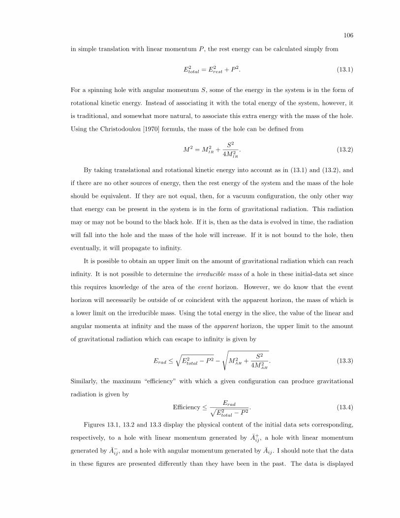
106

in simple translation with linear momentum P , the rest energy can be calculated simply from

E2total = E2

rest + P 2. (13.1)

For a spinning hole with angular momentum S, some of the energy in the system is in the form of

rotational kinetic energy. Instead of associating it with the total energy of the system, however, it

is traditional, and somewhat more natural, to associate this extra energy with the mass of the hole.

Using the Christodoulou [1970] formula, the mass of the hole can be defined from

M2 = M2IR +

S2

4M2IR

. (13.2)

By taking translational and rotational kinetic energy into account as in (13.1) and (13.2), and

if there are no other sources of energy, then the rest energy of the system and the mass of the hole

should be equivalent. If they are not equal, then, for a vacuum configuration, the only other way

that energy can be present in the system is in the form of gravitational radiation. This radiation

may or may not be bound to the black hole. If it is, then as the data is evolved in time, the radiation

will fall into the hole and the mass of the hole will increase. If it is not bound to the hole, then

eventually, it will propagate to infinity.

It is possible to obtain an upper limit on the amount of gravitational radiation which can reach

infinity. It is not possible to determine the irreducible mass of a hole in these initial-data set since

this requires knowledge of the area of the event horizon. However, we do know that the event

horizon will necessarily be outside of or coincident with the apparent horizon, the mass of which is

a lower limit on the irreducible mass. Using the total energy in the slice, the value of the linear and

angular momenta at infinity and the mass of the apparent horizon, the upper limit to the amount

of gravitational radiation which can escape to infinity is given by

Erad ≤√E2total − P 2 −

√M2

AH +S2

4M2AH

. (13.3)

Similarly, the maximum “efficiency” with which a given configuration can produce gravitational

radiation is given by

Efficiency ≤ Erad√E2total − P 2

. (13.4)

Figures 13.1, 13.2 and 13.3 display the physical content of the initial data sets corresponding,

respectively, to a hole with linear momentum generated by A+ij , a hole with linear momentum

generated by A−ij , and a hole with angular momentum generated by Aij . I should note that the data

in these figures are presented differently than they have been in the past. The data is displayed

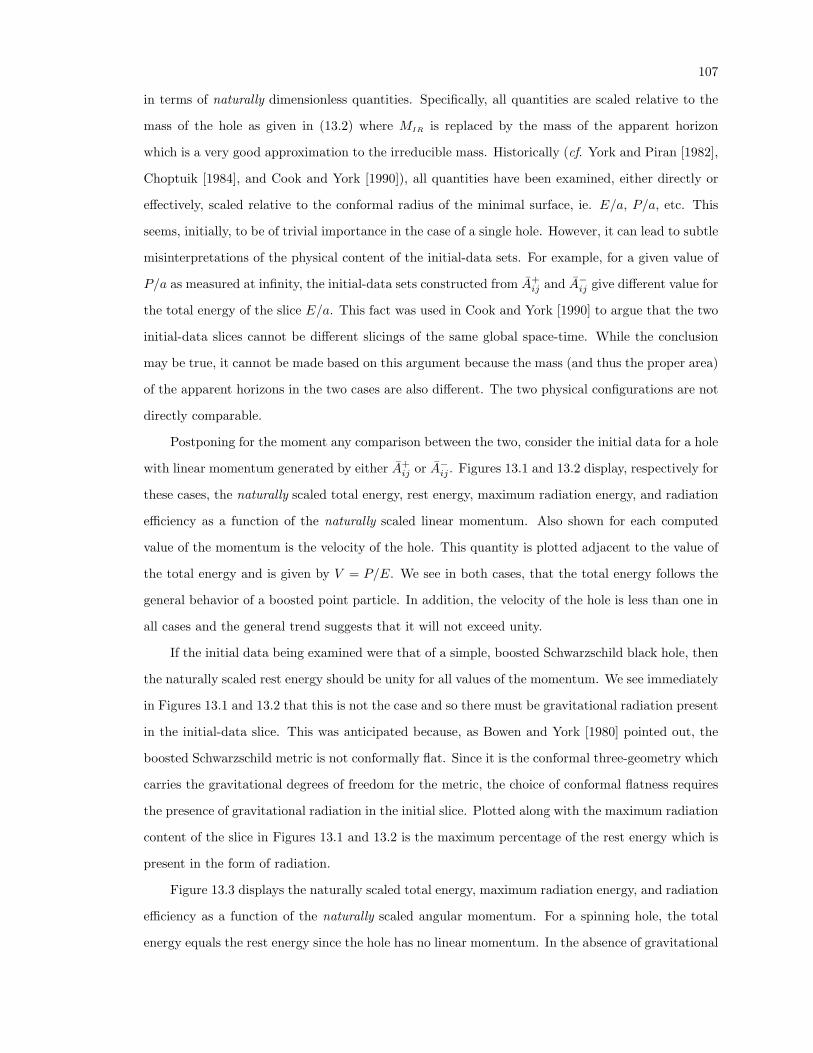
107

in terms of naturally dimensionless quantities. Specifically, all quantities are scaled relative to the

mass of the hole as given in (13.2) where MIR is replaced by the mass of the apparent horizon

which is a very good approximation to the irreducible mass. Historically (cf. York and Piran [1982],

Choptuik [1984], and Cook and York [1990]), all quantities have been examined, either directly or

effectively, scaled relative to the conformal radius of the minimal surface, ie. E/a, P/a, etc. This

seems, initially, to be of trivial importance in the case of a single hole. However, it can lead to subtle

misinterpretations of the physical content of the initial-data sets. For example, for a given value of

P/a as measured at infinity, the initial-data sets constructed from A+ij and A−ij give different value for

the total energy of the slice E/a. This fact was used in Cook and York [1990] to argue that the two

initial-data slices cannot be different slicings of the same global space-time. While the conclusion

may be true, it cannot be made based on this argument because the mass (and thus the proper area)

of the apparent horizons in the two cases are also different. The two physical configurations are not

directly comparable.

Postponing for the moment any comparison between the two, consider the initial data for a hole

with linear momentum generated by either A+ij or A−ij . Figures 13.1 and 13.2 display, respectively for

these cases, the naturally scaled total energy, rest energy, maximum radiation energy, and radiation

efficiency as a function of the naturally scaled linear momentum. Also shown for each computed

value of the momentum is the velocity of the hole. This quantity is plotted adjacent to the value of

the total energy and is given by V = P/E. We see in both cases, that the total energy follows the

general behavior of a boosted point particle. In addition, the velocity of the hole is less than one in

all cases and the general trend suggests that it will not exceed unity.

If the initial data being examined were that of a simple, boosted Schwarzschild black hole, then

the naturally scaled rest energy should be unity for all values of the momentum. We see immediately

in Figures 13.1 and 13.2 that this is not the case and so there must be gravitational radiation present

in the initial-data slice. This was anticipated because, as Bowen and York [1980] pointed out, the

boosted Schwarzschild metric is not conformally flat. Since it is the conformal three-geometry which

carries the gravitational degrees of freedom for the metric, the choice of conformal flatness requires

the presence of gravitational radiation in the initial slice. Plotted along with the maximum radiation

content of the slice in Figures 13.1 and 13.2 is the maximum percentage of the rest energy which is

present in the form of radiation.

Figure 13.3 displays the naturally scaled total energy, maximum radiation energy, and radiation

efficiency as a function of the naturally scaled angular momentum. For a spinning hole, the total

energy equals the rest energy since the hole has no linear momentum. In the absence of gravitational

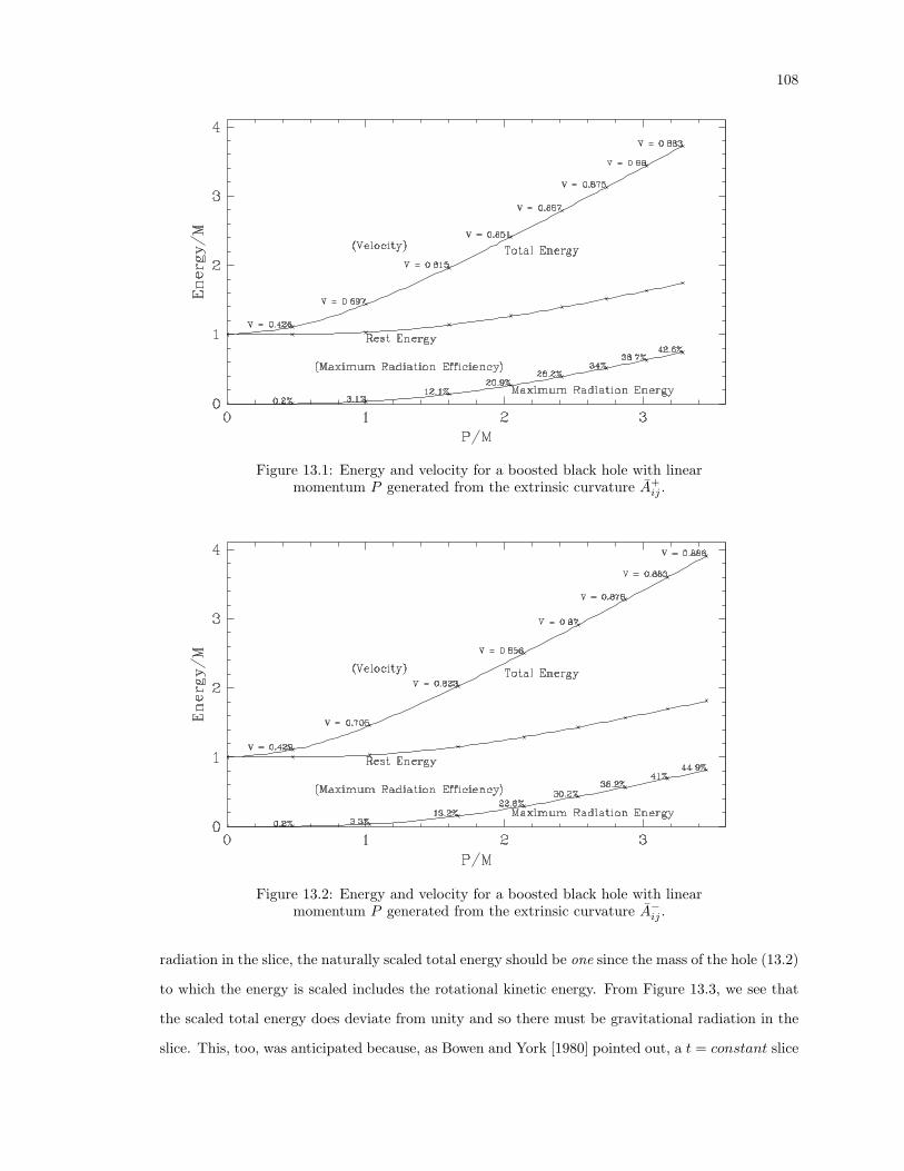
108

1Figure 13.1: Energy and velocity for a boosted black hole with linearmomentum P generated from the extrinsic curvature A+

ij .

1Figure 13.2: Energy and velocity for a boosted black hole with linearmomentum P generated from the extrinsic curvature A−ij .

radiation in the slice, the naturally scaled total energy should be one since the mass of the hole (13.2)

to which the energy is scaled includes the rotational kinetic energy. From Figure 13.3, we see that

the scaled total energy does deviate from unity and so there must be gravitational radiation in the

slice. This, too, was anticipated because, as Bowen and York [1980] pointed out, a t = constant slice

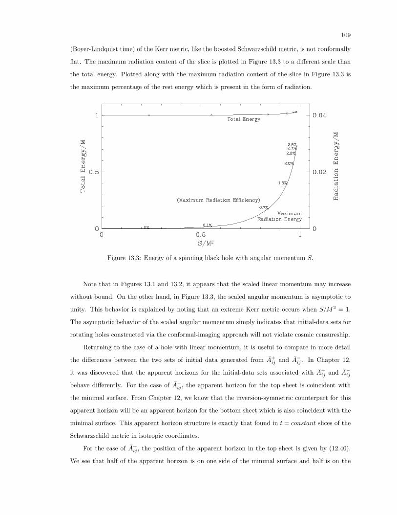
109

(Boyer-Lindquist time) of the Kerr metric, like the boosted Schwarzschild metric, is not conformally

flat. The maximum radiation content of the slice is plotted in Figure 13.3 to a different scale than

the total energy. Plotted along with the maximum radiation content of the slice in Figure 13.3 is

the maximum percentage of the rest energy which is present in the form of radiation.

1Figure 13.3: Energy of a spinning black hole with angular momentum S.

Note that in Figures 13.1 and 13.2, it appears that the scaled linear momentum may increase

without bound. On the other hand, in Figure 13.3, the scaled angular momentum is asymptotic to

unity. This behavior is explained by noting that an extreme Kerr metric occurs when S/M2 = 1.

The asymptotic behavior of the scaled angular momentum simply indicates that initial-data sets for

rotating holes constructed via the conformal-imaging approach will not violate cosmic censureship.

Returning to the case of a hole with linear momentum, it is useful to compare in more detail

the differences between the two sets of initial data generated from A+ij and A−ij . In Chapter 12,

it was discovered that the apparent horizons for the initial-data sets associated with A+ij and A−ij

behave differently. For the case of A−ij , the apparent horizon for the top sheet is coincident with

the minimal surface. From Chapter 12, we know that the inversion-symmetric counterpart for this

apparent horizon will be an apparent horizon for the bottom sheet which is also coincident with the

minimal surface. This apparent horizon structure is exactly that found in t = constant slices of the

Schwarzschild metric in isotropic coordinates.

For the case of A+ij , the position of the apparent horizon in the top sheet is given by (12.40).

We see that half of the apparent horizon is on one side of the minimal surface and half is on the

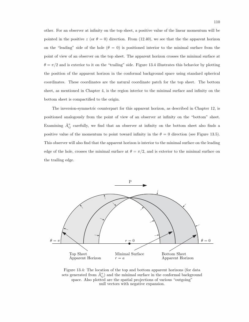
110

other. For an observer at infinity on the top sheet, a positive value of the linear momentum will be

pointed in the positive z (or θ = 0) direction. From (12.40), we see that the the apparent horizon

on the “leading” side of the hole (θ = 0) is positioned interior to the minimal surface from the

point of view of an observer on the top sheet. The apparent horizon crosses the minimal surface at

θ = π/2 and is exterior to it on the “trailing” side. Figure 13.4 illustrates this behavior by plotting

the position of the apparent horizon in the conformal background space using standard spherical

coordinates. These coordinates are the natural coordinate patch for the top sheet. The bottom

sheet, as mentioned in Chapter 4, is the region interior to the minimal surface and infinity on the

bottom sheet is compactified to the origin.

The inversion-symmetric counterpart for this apparent horizon, as described in Chapter 12, is

positioned analogously from the point of view of an observer at infinity on the “bottom” sheet.

Examining A+ij carefully, we find that an observer at infinity on the bottom sheet also finds a

positive value of the momentum to point toward infinity in the θ = 0 direction (see Figure 13.5).

This observer will also find that the apparent horizon is interior to the minimal surface on the leading

edge of the hole, crosses the minimal surface at θ = π/2, and is exterior to the minimal surface on

the trailing edge.

P

θ = 0θ = π r = 0

Top SheetApparent Horizon

Bottom SheetApparent Horizon

Minimal Surfacer = a

1Figure 13.4: The location of the top and bottom apparent horizons (for datasets generated from A+

ij) and the minimal surface in the conformal backgroundspace. Also plotted are the spatial projections of various “outgoing”

null vectors with negative expansion.

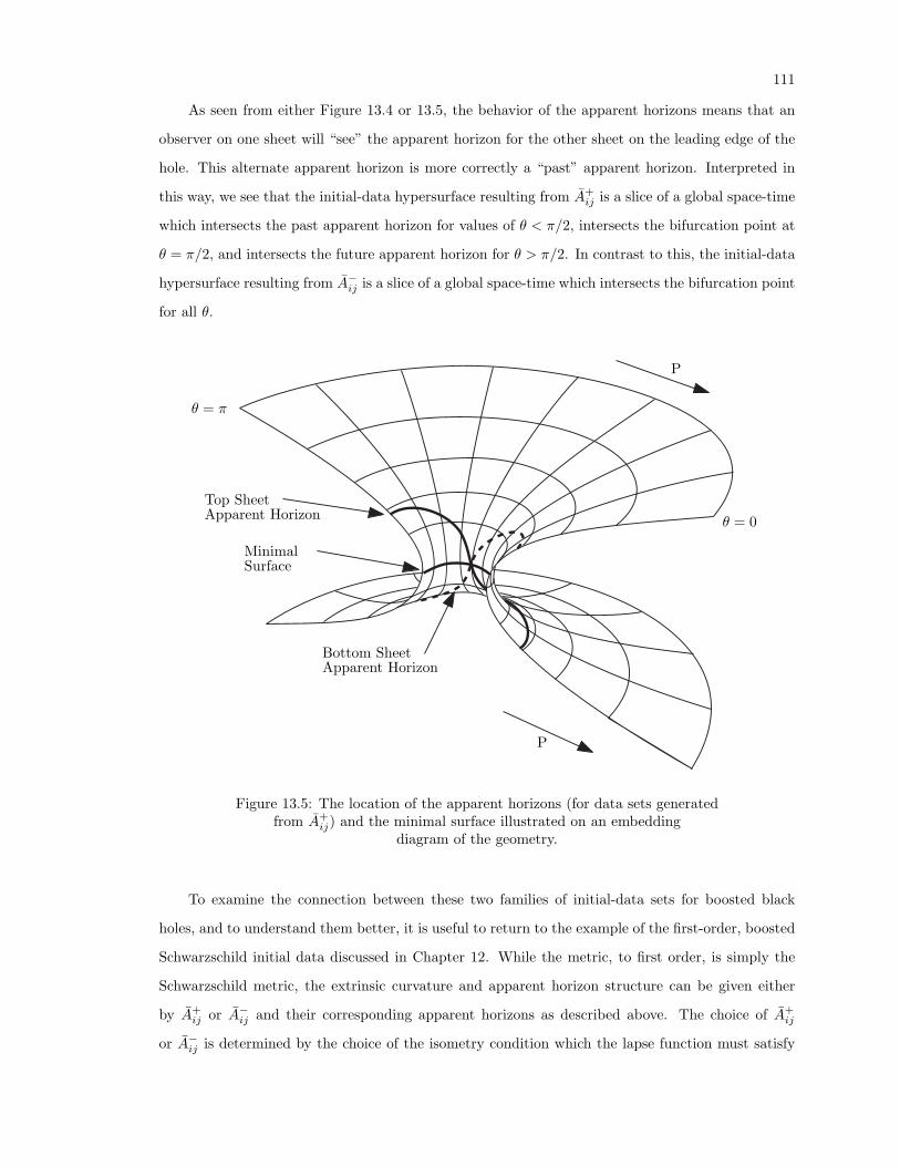
111

As seen from either Figure 13.4 or 13.5, the behavior of the apparent horizons means that an

observer on one sheet will “see” the apparent horizon for the other sheet on the leading edge of the

hole. This alternate apparent horizon is more correctly a “past” apparent horizon. Interpreted in

this way, we see that the initial-data hypersurface resulting from A+ij is a slice of a global space-time

which intersects the past apparent horizon for values of θ < π/2, intersects the bifurcation point at

θ = π/2, and intersects the future apparent horizon for θ > π/2. In contrast to this, the initial-data

hypersurface resulting from A−ij is a slice of a global space-time which intersects the bifurcation point

for all θ.

P

P

θ = 0

θ = π

Top SheetApparent Horizon

Bottom SheetApparent Horizon

MinimalSurface

1Figure 13.5: The location of the apparent horizons (for data sets generatedfrom A+

ij) and the minimal surface illustrated on an embeddingdiagram of the geometry.

To examine the connection between these two families of initial-data sets for boosted black

holes, and to understand them better, it is useful to return to the example of the first-order, boosted

Schwarzschild initial data discussed in Chapter 12. While the metric, to first order, is simply the

Schwarzschild metric, the extrinsic curvature and apparent horizon structure can be given either

by A+ij or A−ij and their corresponding apparent horizons as described above. The choice of A+

ij

or A−ij is determined by the choice of the isometry condition which the lapse function must satisfy

112

and thus, the isometry condition which the extrinsic curvatures must satisfy. In the case of these

first-order initial-data sets, we find that the choice of the isometry condition simply distinguishes

two different maximal slices of the same global space-time and the evolution of either initial-data

set must generate the same global space-time.

The question now is whether or not the two initial data sets given by A+ij or A−ij and their

respective solutions of the Hamiltonian constraint are two different slicings of the same global space-

time. Cook and York [1990] concluded that this was not the case since the total energy for the two

cases, with the same linear momentum, were different. As I have discussed above, this conclusion

cannot be made on this basis. If the naturally scaled initial data is compared by using cubic-spline

interpolation to facilitate a direct comparison, then one finds that the scaled energies differ on at

a level of less than 0.1%. This level of error is too close to the level of the discretization error in

the solution for a conclusion to be drawn. This question may only be answerable by evolving the

initial-data sets and examining the gravitational radiation emitted during the two evolutions.

The apparent-horizon structure found for the A+ij initial data in Chapter 12, in addition to

illuminating the structure of the initial-data slice, also lends support to the use of the conformal

imaging approach. As mentioned in Chapter 4, Thornburg [1987] has proposed using N + 1 sheeted

initial-data hypersurfaces as opposed to the two sheeted initial-data hypersurfaces of the conformal

imaging approach. The use of these hypersurfaces is accompanied by the use of an apparent-horizon

inner boundary condition in place of the minimal surface boundary condition of the conformal

imaging approach. By using the apparent-horizon boundary condition, no information about the

geometry interior to the apparent horizon can be determined. It is argued that this information is

irrelevant since no information can propagate through the apparent horizon and so it can have no

effect on the future evolution of the initial data. What this argument ignores, however, is the fact

that the geometry interior to the apparent horizon does affect the exterior geometry in the sense

that they are both part of a global construction. We see from the example of the apparent horizon

structure for A+ij that knowing only the incomplete initial data exterior to the apparent horizon

would not allow the past apparent horizon to be found. The construction of initial data sets on

complete manifolds is crucial to assuring that the maximum amount of information can be extracted

both from the initial-data set and from its evolution.

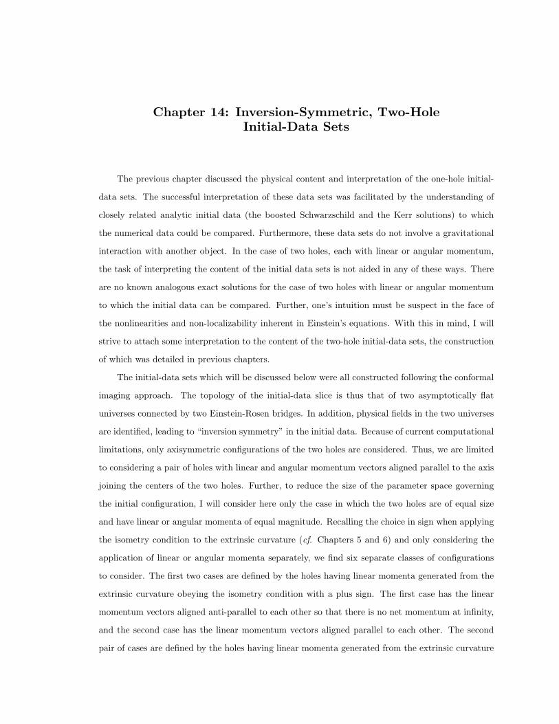
Chapter 14: Inversion-Symmetric, Two-HoleInitial-Data Sets

The previous chapter discussed the physical content and interpretation of the one-hole initial-

data sets. The successful interpretation of these data sets was facilitated by the understanding of

closely related analytic initial data (the boosted Schwarzschild and the Kerr solutions) to which

the numerical data could be compared. Furthermore, these data sets do not involve a gravitational

interaction with another object. In the case of two holes, each with linear or angular momentum,

the task of interpreting the content of the initial data sets is not aided in any of these ways. There

are no known analogous exact solutions for the case of two holes with linear or angular momentum

to which the initial data can be compared. Further, one’s intuition must be suspect in the face of

the nonlinearities and non-localizability inherent in Einstein’s equations. With this in mind, I will

strive to attach some interpretation to the content of the two-hole initial-data sets, the construction

of which was detailed in previous chapters.

The initial-data sets which will be discussed below were all constructed following the conformal

imaging approach. The topology of the initial-data slice is thus that of two asymptotically flat

universes connected by two Einstein-Rosen bridges. In addition, physical fields in the two universes

are identified, leading to “inversion symmetry” in the initial data. Because of current computational

limitations, only axisymmetric configurations of the two holes are considered. Thus, we are limited

to considering a pair of holes with linear and angular momentum vectors aligned parallel to the axis

joining the centers of the two holes. Further, to reduce the size of the parameter space governing

the initial configuration, I will consider here only the case in which the two holes are of equal size

and have linear or angular momenta of equal magnitude. Recalling the choice in sign when applying

the isometry condition to the extrinsic curvature (cf. Chapters 5 and 6) and only considering the

application of linear or angular momenta separately, we find six separate classes of configurations

to consider. The first two cases are defined by the holes having linear momenta generated from the

extrinsic curvature obeying the isometry condition with a plus sign. The first case has the linear

momentum vectors aligned anti-parallel to each other so that there is no net momentum at infinity,

and the second case has the linear momentum vectors aligned parallel to each other. The second

pair of cases are defined by the holes having linear momenta generated from the extrinsic curvature

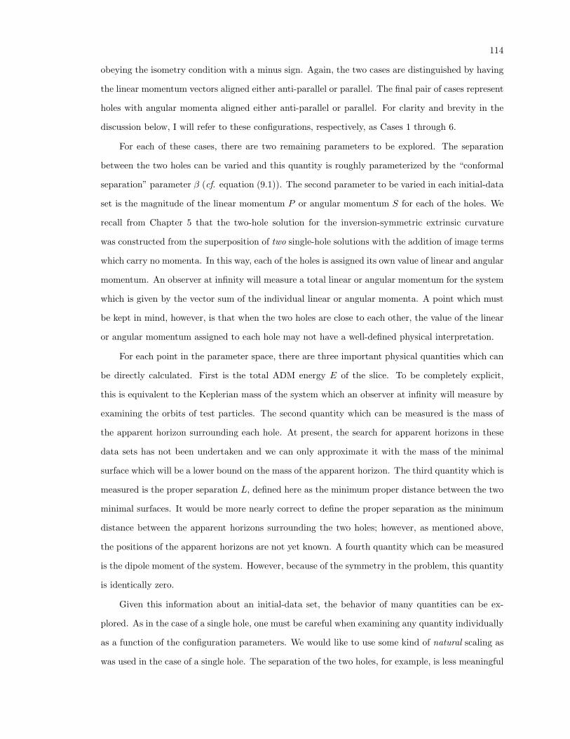
114

obeying the isometry condition with a minus sign. Again, the two cases are distinguished by having

the linear momentum vectors aligned either anti-parallel or parallel. The final pair of cases represent

holes with angular momenta aligned either anti-parallel or parallel. For clarity and brevity in the

discussion below, I will refer to these configurations, respectively, as Cases 1 through 6.

For each of these cases, there are two remaining parameters to be explored. The separation

between the two holes can be varied and this quantity is roughly parameterized by the “conformal

separation” parameter β (cf. equation (9.1)). The second parameter to be varied in each initial-data

set is the magnitude of the linear momentum P or angular momentum S for each of the holes. We

recall from Chapter 5 that the two-hole solution for the inversion-symmetric extrinsic curvature

was constructed from the superposition of two single-hole solutions with the addition of image terms

which carry no momenta. In this way, each of the holes is assigned its own value of linear and angular

momentum. An observer at infinity will measure a total linear or angular momentum for the system

which is given by the vector sum of the individual linear or angular momenta. A point which must

be kept in mind, however, is that when the two holes are close to each other, the value of the linear

or angular momentum assigned to each hole may not have a well-defined physical interpretation.

For each point in the parameter space, there are three important physical quantities which can

be directly calculated. First is the total ADM energy E of the slice. To be completely explicit,

this is equivalent to the Keplerian mass of the system which an observer at infinity will measure by

examining the orbits of test particles. The second quantity which can be measured is the mass of

the apparent horizon surrounding each hole. At present, the search for apparent horizons in these

data sets has not been undertaken and we can only approximate it with the mass of the minimal

surface which will be a lower bound on the mass of the apparent horizon. The third quantity which is

measured is the proper separation L, defined here as the minimum proper distance between the two

minimal surfaces. It would be more nearly correct to define the proper separation as the minimum

distance between the apparent horizons surrounding the two holes; however, as mentioned above,

the positions of the apparent horizons are not yet known. A fourth quantity which can be measured

is the dipole moment of the system. However, because of the symmetry in the problem, this quantity

is identically zero.

Given this information about an initial-data set, the behavior of many quantities can be ex-

plored. As in the case of a single hole, one must be careful when examining any quantity individually

as a function of the configuration parameters. We would like to use some kind of natural scaling as

was used in the case of a single hole. The separation of the two holes, for example, is less meaningful

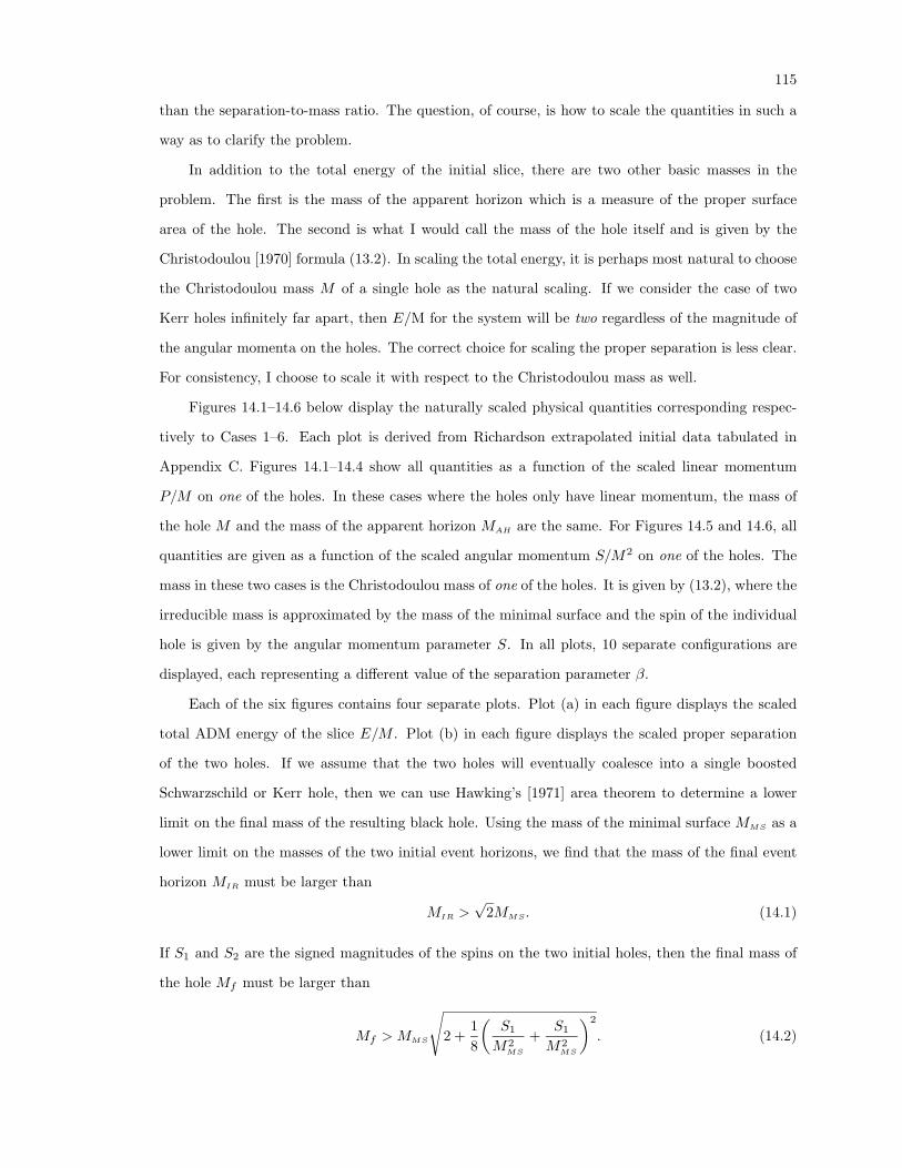
115

than the separation-to-mass ratio. The question, of course, is how to scale the quantities in such a

way as to clarify the problem.

In addition to the total energy of the initial slice, there are two other basic masses in the

problem. The first is the mass of the apparent horizon which is a measure of the proper surface

area of the hole. The second is what I would call the mass of the hole itself and is given by the

Christodoulou [1970] formula (13.2). In scaling the total energy, it is perhaps most natural to choose

the Christodoulou mass M of a single hole as the natural scaling. If we consider the case of two

Kerr holes infinitely far apart, then E/M for the system will be two regardless of the magnitude of

the angular momenta on the holes. The correct choice for scaling the proper separation is less clear.

For consistency, I choose to scale it with respect to the Christodoulou mass as well.

Figures 14.1–14.6 below display the naturally scaled physical quantities corresponding respec-

tively to Cases 1–6. Each plot is derived from Richardson extrapolated initial data tabulated in

Appendix C. Figures 14.1–14.4 show all quantities as a function of the scaled linear momentum

P/M on one of the holes. In these cases where the holes only have linear momentum, the mass of

the hole M and the mass of the apparent horizon MAH are the same. For Figures 14.5 and 14.6, all

quantities are given as a function of the scaled angular momentum S/M2 on one of the holes. The

mass in these two cases is the Christodoulou mass of one of the holes. It is given by (13.2), where the

irreducible mass is approximated by the mass of the minimal surface and the spin of the individual

hole is given by the angular momentum parameter S. In all plots, 10 separate configurations are

displayed, each representing a different value of the separation parameter β.

Each of the six figures contains four separate plots. Plot (a) in each figure displays the scaled

total ADM energy of the slice E/M . Plot (b) in each figure displays the scaled proper separation

of the two holes. If we assume that the two holes will eventually coalesce into a single boosted

Schwarzschild or Kerr hole, then we can use Hawking’s [1971] area theorem to determine a lower

limit on the final mass of the resulting black hole. Using the mass of the minimal surface MMS as a

lower limit on the masses of the two initial event horizons, we find that the mass of the final event

horizon MIR must be larger than

MIR >√

2MMS. (14.1)

If S1 and S2 are the signed magnitudes of the spins on the two initial holes, then the final mass of

the hole Mf must be larger than

Mf > MMS

√2 +

18

(S1

M2MS

+S1

M2MS

)2

. (14.2)

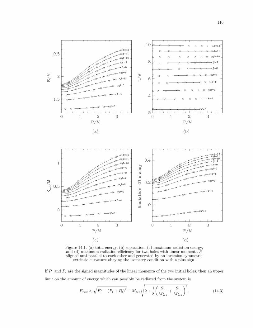
116

1Figure 14.1: (a) total energy, (b) separation, (c) maximum radiation energy,and (d) maximum radiation efficiency for two holes with linear momenta Paligned anti-parallel to each other and generated by an inversion-symmetric

extrinsic curvature obeying the isometry condition with a plus sign.

If P1 and P2 are the signed magnitudes of the linear momenta of the two initial holes, then an upper

limit on the amount of energy which can possibly be radiated from the system is

Erad <

√E2 − (P1 + P2)2 −MMS

√2 +

18

(S1

M2MS

+S1

M2MS

)2

. (14.3)

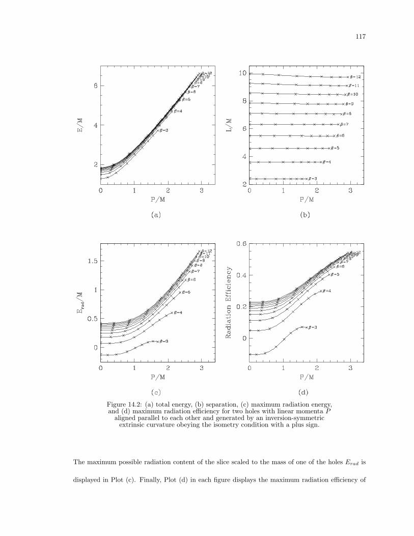
117

1Figure 14.2: (a) total energy, (b) separation, (c) maximum radiation energy,and (d) maximum radiation efficiency for two holes with linear momenta P

aligned parallel to each other and generated by an inversion-symmetricextrinsic curvature obeying the isometry condition with a plus sign.

The maximum possible radiation content of the slice scaled to the mass of one of the holes Erad is

displayed in Plot (c). Finally, Plot (d) in each figure displays the maximum radiation efficiency of

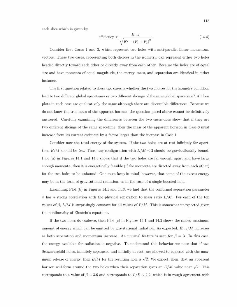
118

each slice which is given by

efficiency <Erad√

E2 − (P1 + P2)2. (14.4)

Consider first Cases 1 and 3, which represent two holes with anti-parallel linear momentum

vectors. These two cases, representing both choices in the isometry, can represent either two holes

headed directly toward each other or directly away from each other. Because the holes are of equal

size and have momenta of equal magnitude, the energy, mass, and separation are identical in either

instance.

The first question related to these two cases is whether the two choices for the isometry condition

lead to two different global spacetimes or two different slicings of the same global spacetime? All four

plots in each case are qualitatively the same although there are discernible differences. Because we

do not know the true mass of the apparent horizon, the question posed above cannot be definitively

answered. Carefully examining the differences between the two cases does show that if they are

two different slicings of the same spacetime, then the mass of the apparent horizon in Case 3 must

increase from its current estimate by a factor larger than the increase in Case 1.

Consider now the total energy of the system. If the two holes are at rest infinitely far apart,

then E/M should be two. Thus, any configuration with E/M < 2 should be gravitationally bound.

Plot (a) in Figures 14.1 and 14.3 shows that if the two holes are far enough apart and have large

enough momenta, then it is energetically feasible (if the momenta are directed away from each other)

for the two holes to be unbound. One must keep in mind, however, that some of the excess energy

may be in the form of gravitational radiation, as in the case of a single boosted hole.

Examining Plot (b) in Figures 14.1 and 14.3, we find that the conformal separation parameter

β has a strong correlation with the physical separation to mass ratio L/M . For each of the ten

values of β, L/M is surprisingly constant for all values of P/M . This is somewhat unexpected given

the nonlinearity of Einstein’s equations.

If the two holes do coalesce, then Plot (c) in Figures 14.1 and 14.2 shows the scaled maximum

amount of energy which can be emitted by gravitational radiation. As expected, Erad/M increases

as both separation and momentum increase. An unusual feature is seen for β = 3. In this case,

the energy available for radiation is negative. To understand this behavior we note that if two

Schwarzschild holes, infinitely separated and initially at rest, are allowed to coalesce with the max-

imum release of energy, then E/M for the resulting hole is√

2. We expect, then, that an apparent

horizon will form around the two holes when their separation gives an E/M value near√

2. This

corresponds to a value of β ∼ 3.6 and corresponds to L/E ∼ 2.2, which is in rough agreement with

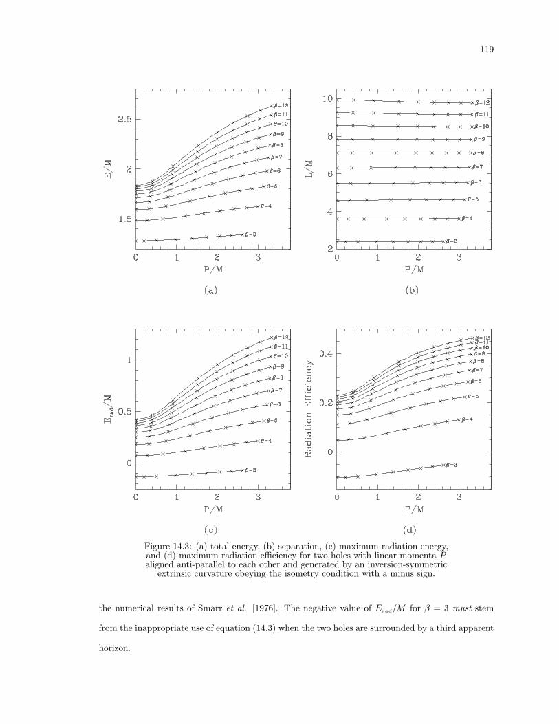
119

1Figure 14.3: (a) total energy, (b) separation, (c) maximum radiation energy,and (d) maximum radiation efficiency for two holes with linear momenta Paligned anti-parallel to each other and generated by an inversion-symmetric

extrinsic curvature obeying the isometry condition with a minus sign.

the numerical results of Smarr et al. [1976]. The negative value of Erad/M for β = 3 must stem

from the inappropriate use of equation (14.3) when the two holes are surrounded by a third apparent

horizon.

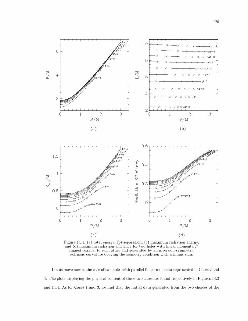
120

1Figure 14.4: (a) total energy, (b) separation, (c) maximum radiation energy,and (d) maximum radiation efficiency for two holes with linear momenta P

aligned parallel to each other and generated by an inversion-symmetricextrinsic curvature obeying the isometry condition with a minus sign.

Let us move now to the case of two holes with parallel linear momenta represented in Cases 2 and

4. The plots displaying the physical content of these two cases are found respectively in Figures 14.2

and 14.4. As for Cases 1 and 3, we find that the initial data generated from the two choices of the

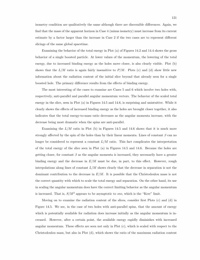
121

isometry condition are qualitatively the same although there are discernible differences. Again, we

find that the mass of the apparent horizon in Case 4 (minus isometry) must increase from its current

estimate by a factor larger than the increase in Case 2 if the two cases are to represent different

slicings of the same global spacetime.

Examining the behavior of the total energy in Plot (a) of Figures 14.2 and 14.4 shows the gross

behavior of a single boosted particle. At lower values of the momentum, the lowering of the total

energy, due to increased binding energy as the holes move closer, is also clearly visible. Plot (b)

shows that the L/M ratio is again fairly insensitive to P/M . Plots (c) and (d) show little new

information about the radiation content of the initial slice beyond that already seen for a single

boosted hole. The primary difference results from the effects of binding energy.

The most interesting of the cases to examine are Cases 5 and 6 which involve two holes with,

respectively, anti-parallel and parallel angular momentum vectors. The behavior of the scaled total

energy in the slice, seen in Plot (a) in Figures 14.5 and 14.6, is surprising and unintuitive. While it

clearly shows the effects of increased binding energy as the holes are brought closer together, it also

indicates that the total energy-to-mass ratio decreases as the angular momenta increase, with the

decrease being most dramatic when the spins are anti-parallel.

Examining the L/M ratio in Plot (b) in Figures 14.5 and 14.6 shows that it is much more

strongly affected by the spin of the holes than by their linear momenta. Lines of constant β can no

longer be considered to represent a constant L/M ratio. This fact complicates the interpretation

of the total energy of the slice seen in Plot (a) in Figures 14.5 and 14.6. Because the holes are

getting closer, for constant β as the angular momenta is increased, they necessarily have a greater

binding energy and the decrease in E/M must be due, in part, to this effect. However, rough

interpolations along lines of constant L/M shows clearly that the decrease in separation is not the

dominant contribution to the decrease in E/M . It is possible that the Christodoulou mass is not

the correct quantity with which to scale the total energy and separation. On the other hand, its use

in scaling the angular momentum does have the correct limiting behavior as the angular momentum

is increased. That is, S/M2 appears to be asymptotic to one, which is the “Kerr” limit.

Moving on to examine the radiation content of the slices, consider first Plots (c) and (d) in

Figure 14.5. We see, in the case of two holes with anti-parallel spins, that the amount of energy

which is potentially available for radiation does increase initially as the angular momentum is in-

creased. However, after a certain point, the available energy rapidly diminishes with increased

angular momentum. These effects are seen not only in Plot (c), which is scaled with respect to the

Christodoulou mass, but also in Plot (d), which shows the ratio of the maximum radiation content

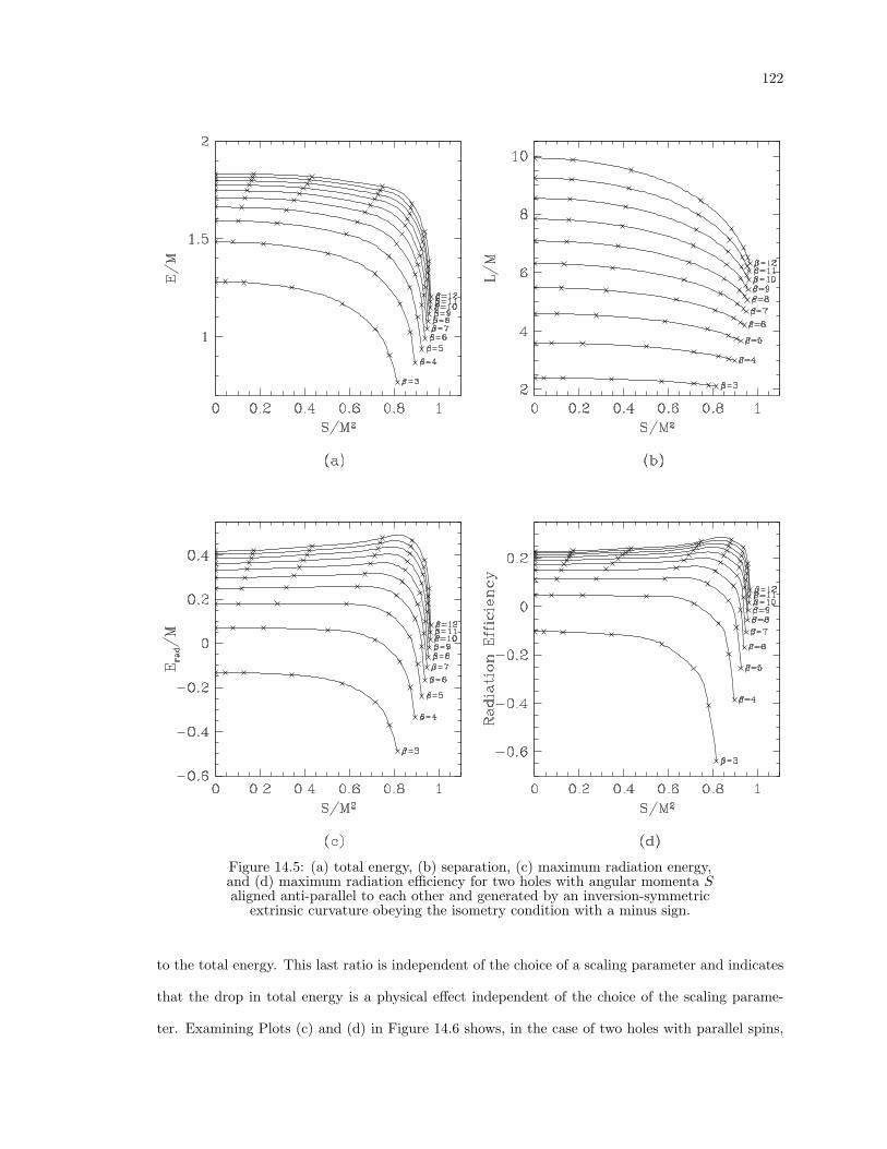
122

1Figure 14.5: (a) total energy, (b) separation, (c) maximum radiation energy,and (d) maximum radiation efficiency for two holes with angular momenta Saligned anti-parallel to each other and generated by an inversion-symmetric

extrinsic curvature obeying the isometry condition with a minus sign.

to the total energy. This last ratio is independent of the choice of a scaling parameter and indicates

that the drop in total energy is a physical effect independent of the choice of the scaling parame-

ter. Examining Plots (c) and (d) in Figure 14.6 shows, in the case of two holes with parallel spins,

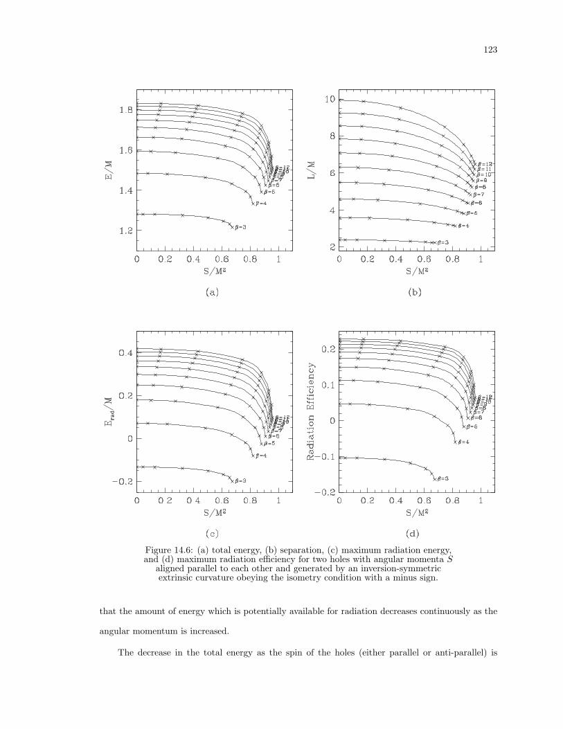
123

1Figure 14.6: (a) total energy, (b) separation, (c) maximum radiation energy,and (d) maximum radiation efficiency for two holes with angular momenta S

aligned parallel to each other and generated by an inversion-symmetricextrinsic curvature obeying the isometry condition with a minus sign.

that the amount of energy which is potentially available for radiation decreases continuously as the

angular momentum is increased.

The decrease in the total energy as the spin of the holes (either parallel or anti-parallel) is

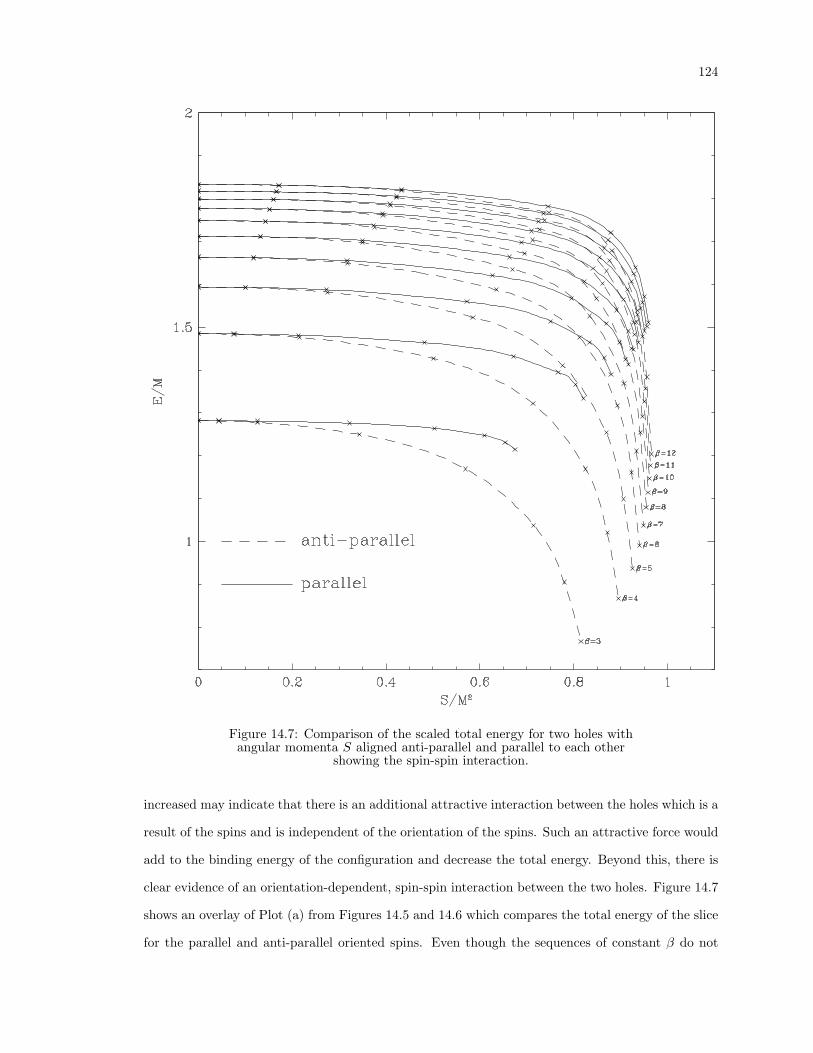
124

1Figure 14.7: Comparison of the scaled total energy for two holes withangular momenta S aligned anti-parallel and parallel to each other

showing the spin-spin interaction.

increased may indicate that there is an additional attractive interaction between the holes which is a

result of the spins and is independent of the orientation of the spins. Such an attractive force would

add to the binding energy of the configuration and decrease the total energy. Beyond this, there is

clear evidence of an orientation-dependent, spin-spin interaction between the two holes. Figure 14.7

shows an overlay of Plot (a) from Figures 14.5 and 14.6 which compares the total energy of the slice

for the parallel and anti-parallel oriented spins. Even though the sequences of constant β do not

125

represent a constant L/M ratio, the L/M curves for constant β are nearly identical for both the

parallel and anti-parallel spin scenarios. This allows us to directly compare the E/M ratio in the

two cases for the same values of β. For each value of β, we find that the E/M ratio is lower when

the spins are oriented anti-parallel than when parallel. This indicates that there is a spin-spin force

which is attractive when the spins are anti-aligned and repulsive when aligned. Such an interaction

is in agreement with the gravitational spin-spin interaction investigated by Wald [1972] for the case

of a spinning test particle in the exterior field of an arbitrary, stationary, rotating source. We can

also see that the magnitude of the spin-spin force decreases as the separation between the holes

increases. This is apparent from the fact that the difference in the energy levels for the aligned and

anti-aligned cases decreases as the separation increases.

As evidenced by the discussion above, the understanding of the content of the two-hole initial-

data sets is far from complete. Many uncertainties should be resolved when the location and areas of

the apparent horizons are determined. This knowledge will allow for much more accurate estimates

of the irreducible mass of the holes and will greatly change many of the estimates for the radiation

content of the initial-data slices since the current method of estimating the radiation content assumes

that there is not a third horizon surrounding both holes. In any case, it will probably be the case

that a complete understanding of the content of these two-hole initial-data sets will be found only

by evolving them in time.

Chapter 15: Conclusion

The primary motivation for undertaking an investigation of methods for computing initial-data

sets containing one or more black holes is the desire to simulate black hole collisions. In particular,

we wish to evolve data which represent two black holes in a bound orbit, spiralling toward a collision.

During this evolution, we wish to examine the gravitational radiation which is being emitted during

the spiralling infall, the collision, and the subsequent transition to quiescence. With this in mind,

I will discuss the usefulness and limitations of initial-data sets constructed following the conformal

imaging approach. I will also discuss some of the problems remaining to be investigated regarding

the generation and evolution of these initial-data sets.

The most obvious advantage of the conformal imaging approach over other methods for con-

structing initial-data sets containing black holes (cf. Thornburg [1987]) is that it allows for the

construction of initial data on a complete manifold. During an evolution of this initial data, more

of the global structure of the space-time should be accessible because the initial-data manifold is

complete. The “price” which is paid for having a complete manifold is that all of the fields which

reside on the manifold must obey an isometry condition which identifies the physical fields on the two

“sheets” (or universes) which the manifold comprises. At first, this identification may seem unnatu-

ral. The imposition of such an isometry condition is possible only when topological vacuum solutions

are considered. If the black hole is produced from a matter source, then there can be no “alternate”

universe to identify with the “physical” universe. The existence of multiple, causally disconnected,

asymptotically flat regions seems to be a generic feature of vacuum black-hole space-times. Unless

there is some reason that these additional universes should be considered physically relevant and dis-

tinct from the “real” universe, it actually seems most natural to identify these causally disconnected

regions mathematically.

One of the most important reasons for pursuing the evolution of the two black hole collision

problem is the desire to obtain accurate waveforms for the gravitational radiation which results from

the collision. In order to be able to compare waveforms generated by numerical means confidently

against waveforms which should be available in the future from gravity-wave detectors, it will be

important to be able to distinguish between waveforms which result from the dynamics of the

127

evolution and those which are present in the initial data. As has been shown, initial-data sets

constructed by the conformal imaging approach must contain gravitational radiation in the field

exterior to the apparent horizon. This is not a condition inherent only to the conformal imaging

approach, however. Any initial-data sets constructed on a space-like slice will most likely contain

gravitational radiation. Even if the trace-free background extrinsic curvature is purely longitudinal,

the physical extrinsic curvature may have a non-vanishing, transverse-traceless part.

Since these initial-data sets do contain gravitational radiation from the start, it will be necessary

to determine its content in some quantitative way so that its contribution to the dynamical waveform

can be determined. It is likely that any gravitational radiation present in the initial slice can be made

to propagate away from or fall into the holes before any of the interesting dynamics takes place. In

addition, some hope for finding methods of examining the gravitational radiation content of initial-

data sets has been expressed by Abrahams [1990] based on experience in extracting waveforms from

numerical evolutions of Einstein’s equations (cf. Abrahams and Evans [1988], [1990]). I feel that

this avenue of investigating the radiation content of the initial data should be vigorously pursued.

Beyond these questions regarding the content of the initial-data sets, there are problems which

have yet to be addressed regarding their numerical generation. The research described in this work

has dealt with the generation of axisymmetric initial-data sets. I have found a general, explicit ap-

proach for evaluating the two-hole, inversion-symmetric extrinsic curvature and I have demonstrated

two approaches for solving the two-hole Hamiltonian constraint numerically. With regard to these

axisymmetric data sets, the task of increasing the accuracy of the numerical solutions still remains

as does the problem of locating the apparent horizons in these data sets.

In order to model the spiralling collision of two black holes, three-dimensional initial-data sets

will be required. Many of the techniques developed for constructing axisymmetric data sets can

be applicable to the three-dimensional problems. The method I have developed for evaluating the

axisymmetric, inversion-symmetric extrinsic curvature is directly generalizable to three-dimensional

situations. The general approaches for differencing the Hamiltonian constraint should also be appli-

cable. However, some effort will be needed with regard to differencing near the coordinate singularity

along the z-axis in the absence of axisymmetry. Also, much work will be required in finding an ef-

ficient approach for solving the resulting difference equations. The size of this set of equations will

be significantly larger than that resulting from differencing the axisymmetric problem and will tax

the memory limitations of even the most powerful supercomputers.

I would like to turn now to the problem of evolving inversion-symmetric initial-data sets. As was

mentioned earlier, the use of initial data on a complete manifold should allow for more of the global

128

space-time to be covered during a numerical evolution. Initial data constructed by the conformal

imaging approach allows for the efficient construction of initial data on a complete manifold because

only half of the full manifold must be considered. The other half is known by identification through

the isometry condition. Because the two sheets of the manifold contain identical Cauchy data, the

two causally disconnected spacetimes which evolve from these data will be identical and there will

therefore exist a spacetime isometry between them. If efficient use is to be made of the initial data,

however, then each spatial slice in the subsequent evolution should also consist of a complete three-

manifold on which the data obey a spatial isometry condition which is either similar or identical to

the isometry condition on the initial-data slice. This means that the question of the compatibility

of the isometry condition and the evolution equations must be considered.

A full investigation of this problem is beyond the scope of this concluding chapter, but I do

wish to discuss some of the more general points. To begin with, all of the fields which are relevant to

the evolution equations will be required to satisfy some isometry condition. The isometry condition

includes, in some cases, the freedom of choice in the sign of the identified field. For example, we

have seen in Chapter 4 that the extrinsic curvature can obey the isometry condition with either a

plus or a minus sign. The metric, on the other hand, must obey the isometry condition only with a

plus sign in order for the metric to be non-singular on the inversion surfaces. To determine the sign

of the isometry condition for the other fields we must examine the vacuum Einstein equations

R+23K2 −AijAij = 0, (15.1)

Dj(Aij −23γijK) = 0, (15.2)

∂tAij =−DiDjα+ αRij − 2αAi`Aj` + αAij(13K) + 3αγij(

13K)2

− γij∂t(13K) + γijβ

`D`(13K) + β`D`Aij +Ai`Djβ

` +A`jDiβ`,

(15.3)

and

∂tγij = −2αAij −23αγijK +Diβj +Djβi. (15.4)

We see immediately that the lapse α and the trace of the extrinsic curvature K must obey the

isometry condition with the same sign as the extrinsic curvature

α(x) = ±α(Jα(x)) (15.5)

and

K(x) = ±K(Jα(x)). (15.6)

129

(The subscript α on the isometry condition Jα designates the throat through which the isometry is

applied and should not be confused with the lapse function.) We also find that the shift vector βi

must obey the isometry condition with the plus sign

βi(x) = (J−1α )j

iβj(Jα(x)). (15.7)

The isometry conditions (15.5)–(15.7) along with similar conditions for the metric and extrinsic

curvature (4.38) and (4.39) can be used to generate boundary conditions which these fields must obey

at the inversion surfaces which are fixed point sets of the isometry. Using the isometry condition

which we know is obeyed on the initial hypersurface and going to a local spherical coordinate system

(r, θ, φ) centered around any given throat, we can read off boundary conditions for each component

of each field. The boundary condition will be such that either the normal derivative of a given

component vanishes at the throat or the value of the component vanishes at the throat. Since there

is no choice in the sign of the isometry condition for the metric, we find immediately that the normal

derivatives of γrr, γθθ, γφφ, and γθφ must vanish at a throat and γrθ and γrφ must vanish in value

at a throat. There is also no choice in the sign of the isometry condition for the shift vector and

we find that βr must vanish in value at a throat and also that the normal derivatives of βθ and

βφ must vanish at a throat. The boundary condition for the remaining quantities depends on the

choice in sign for the isometry condition. If the isometry condition with a plus sign is chosen for α,

K, and Aij , then we find that the normal derivatives of α, K, Arr, Aθθ, Aφφ, and Aθφ must vanish

on a throat and so Arθ and Arφ must vanish in value on a throat. If the isometry condition with a

minus sign is chosen, then the conditions are reversed. Boundary conditions of this sort are being

used by Bernstein and Hobill [1990] in their investigations into the evolution of a single, perturbed

black hole.

We can now consider whether the imposition of these boundary conditions in conjuction with

the evolution equations (15.3) and (15.4) is sufficient to guarantee that the fields on subsequent

slices will be inversion symmetric. The imposition of the boundary conditions described above

should ensure that the surfaces identified with fixed-point sets of the isometry remain fixed-point

sets throughout the evolution. What it may not do, however, is determine what the explicit form

of the isometry conditions (or maps) will be. It is the explicit form of the isometry maps which,

given a coordinate map defined by the isometry, allows for the smooth continuation of fields through

the inversion surfaces. This, in turn, allows global structures such as apparent horizons, which may

cross the inversion surface, to be located.

130

To exploit fully the conformal imaging approach, it will be necessary to understand better the

relation between the isometry maps and the evolution equations, and also their relation with the

constraint equations on evolved slices which will not be conformally flat. While I do not claim to

have come to any complete understanding of this problem, I would like to discuss a few important

points. It seems likely to me that the explicit form of the isometry condition will be dependent

on the choice of the shift vector. This can be seen from the fact that the isometry condition is

defined to identify points in the two identical sheets which the manifold comprises. Since the shift

vector determines which coordinate point is associated with a physical point in the manifold, it must

be closely associated with the evolution of the isometry condition. Another point of consideration

is the connection between the isometry condition and the choice of hypersurfaces throughout the

evolution. It is evident that not just any general hypersurface will allow for the identification of

data in the two sheets. Thus, the choice of the lapse function must be made in such a way which

as to be compatible with the isometry. Some clue to possible constraints on the choice of the lapse

function may be found in the evolution equations.

A clear understanding of the relationships mentioned above will be very important to our

undertaking of the evolution of these inversion-symmetric initial-data sets. A successful combination

of isometry conditions and the evolution equations will allow for evolution on complete manifolds

which I feel will be of benefit. We know implicitly, from the uniqueness of the evolution of the

Cauchy data, that the two universes are identical. What technical difficulties exist in finding an

explicit, spatial isometry condition remain to be determined. In any event, it is clear that the work

presented here is but a small part of the effort which will be required in the quest for the evolution

of a spiralling binary coalescence.

Appendix A: The Multigrid Algorithm

The problem of numerically solving an elliptic boundary value problem is usually reduced to

the problem of solving a large matrix equation. The task of solving this system of equations can

be handled in a variety of ways. The equations can be solved by direct matrix inversion or by

iterative techniques. The accuracy of direct solutions is usually limited by the computational storage

requirements of large matrices, although the number of computational operations is also a limiting

factor. For iterative schemes, it is the number of computational operations which usually limits the

accuracy of solutions. Some of the most promising approaches for bypassing the time and memory

problems and finding fast, accurate solutions are offered by multigrid techniques (cf. Brandt [1977],

Hackbusch and Trottenberg [1982], Choptuik [1982], Hackbusch [1985], Choptuik and Unruh [1986],

and Cook [1989]).

Probably the most widely used multigrid algorithm for non-linear problems is the full approxi-

mation storage (FAS) algorithm proposed by Brandt [1977]. Its use in numerical relativity has been

advocated by Choptuik and Unruh [1986] and Cook [1989]. The following discussion closely follows

Cook [1989].

Let the differential equation to be solved be denoted by

Fϕ = f, (A.1)

where F is a non-linear differential operator acting on ϕ, and f is a source term. Now let Pk be

an operator which projects a scalar function onto a discrete mesh Mk labeled by k and covering

the computational domain. The representation of the source function f on the mesh Mk is thus

Pkf = fk. The finite difference approximation of (A.1) on Mk will be denoted by

Fkϕk = fk. (A.2)

Fk is the set of possibly non-linear algebraic equations obtained from finite differencing F and

ϕk 6= Pkϕ since ϕk is the set of values which must satisfy the difference equations (A.2). The

difference ϕk−Pkϕ is known as the discretization error in the solution and results from the truncation

132

error inherent in the finite difference approximation. The local truncation error τk of the finite

difference operator Fk is given by

τk ≡ Fk(Pkϕ)− fk = Fk(Pkϕ)− Pk(Fϕ). (A.3)

If, somehow, τk could be found without knowing the exact solution ϕ, then the solution to

Fkϕk = fk + τk (A.4)

would be the projection of the exact solution ϕ and there would be no discretization error.

While it is not possible, in general, to determine τk exactly, there is a great deal of information

about the discretization which is not used in traditional direct or iterative solution techniques which

can be used to approximate τk. Consider two different discretizations of the computational domain,

Mk and Mk−1, where the discretization of Mk−1 is coarser than that of Mk. Now define two

operators which smoothly interpolate values from one mesh to the other. The prolongation operator

Ikk−1 takes values from the coarse mesh to the finer mesh, and the restriction operator Ik−1k takes

values from the fine mesh to the coarse mesh. If we have a solution on the fine mesh satisfying (A.2),

then we can define, in a manner similar to (A.3), the relative local truncation error τk−1k

τk−1k ≡ Fk−1(Ik−1

k ϕk)− Ik−1k (Fkϕk). (A.5)

The relative local truncation error can be used as an estimate of the local truncation error of the

difference operator on Mk−1. If we now solve

F k−1ϕk−1 = fk−1 + τk−1k , (A.6)

then ϕk−1 will be a better approximation of Pk−1ϕ since the discretization error of (A.6) will be on

the order of that on Mk, as opposed to that on Mk−1.

To this point, solving (A.6) does not aid in the solution of the problem onMk since the solution

on Mk was needed to generate τk−1k . To proceed, instead of using an actual solution to (A.2) in

(A.5) consider ϕk now to be only an approximate solution. If the approximate solution is sufficiently

close to the true solution, then the solution to (A.6) will be a good approximation of the solution

to (A.2) and, since (A.6) is defined on the coarser mesh, it will require less work than (A.2) to

solve. Once the solution ϕk−1 is known, then subtracting Ik−1k ϕk gives the amount by which the

approximate solution on Mk has been corrected. The coarse grid correction is thus defined as

ϕk−1 − Ik−1k ϕk. (A.7)

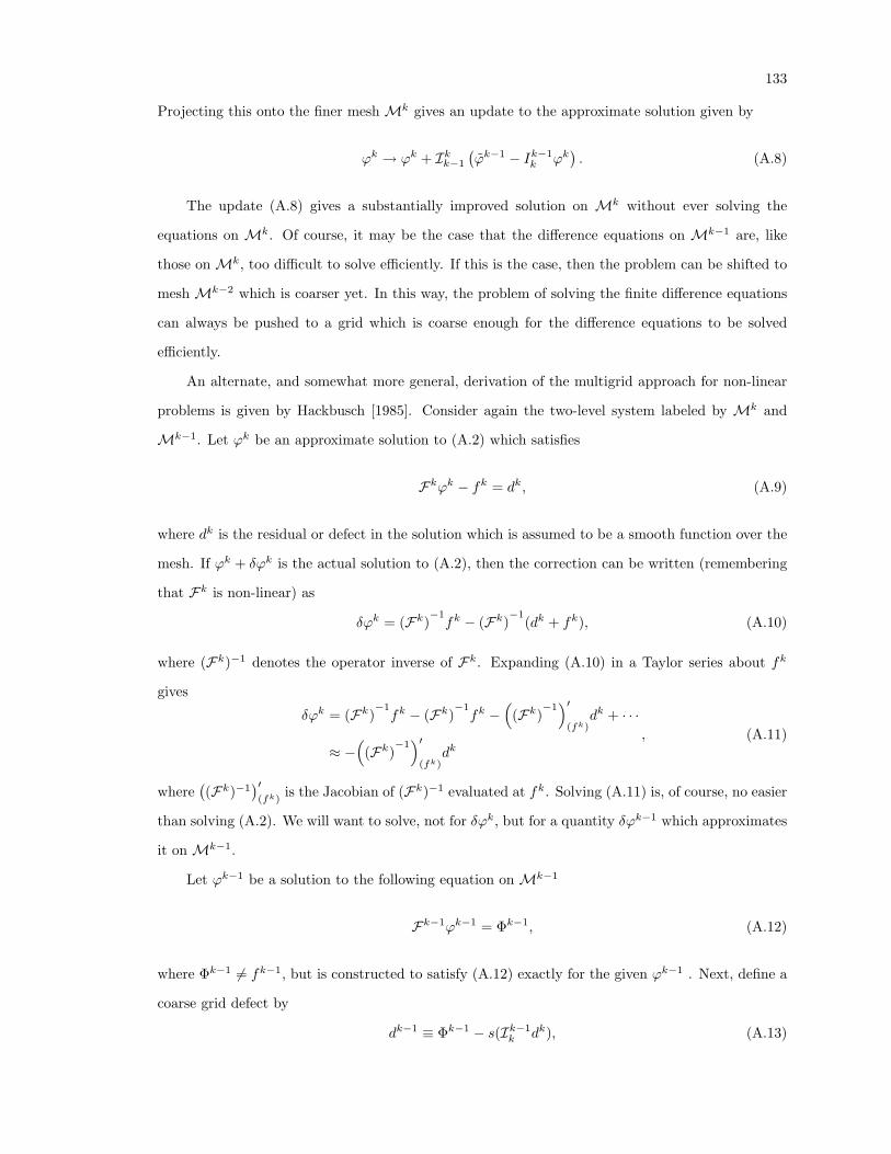
133

Projecting this onto the finer mesh Mk gives an update to the approximate solution given by

ϕk → ϕk + Ikk−1

(ϕk−1 − Ik−1

k ϕk). (A.8)

The update (A.8) gives a substantially improved solution on Mk without ever solving the

equations on Mk. Of course, it may be the case that the difference equations on Mk−1 are, like

those on Mk, too difficult to solve efficiently. If this is the case, then the problem can be shifted to

mesh Mk−2 which is coarser yet. In this way, the problem of solving the finite difference equations

can always be pushed to a grid which is coarse enough for the difference equations to be solved

efficiently.

An alternate, and somewhat more general, derivation of the multigrid approach for non-linear

problems is given by Hackbusch [1985]. Consider again the two-level system labeled by Mk and

Mk−1. Let ϕk be an approximate solution to (A.2) which satisfies

Fkϕk − fk = dk, (A.9)

where dk is the residual or defect in the solution which is assumed to be a smooth function over the

mesh. If ϕk + δϕk is the actual solution to (A.2), then the correction can be written (remembering

that Fk is non-linear) as

δϕk = (Fk)−1fk − (Fk)

−1(dk + fk), (A.10)

where (Fk)−1 denotes the operator inverse of Fk. Expanding (A.10) in a Taylor series about fk

gives

δϕk = (Fk)−1fk − (Fk)

−1fk −

((Fk)

−1)′

(fk)dk + · · ·

≈ −(

(Fk)−1)′

(fk)dk

, (A.11)

where((Fk)−1

)′(fk)

is the Jacobian of (Fk)−1 evaluated at fk. Solving (A.11) is, of course, no easier

than solving (A.2). We will want to solve, not for δϕk, but for a quantity δϕk−1 which approximates

it on Mk−1.

Let ϕk−1 be a solution to the following equation on Mk−1

Fk−1ϕk−1 = Φk−1, (A.12)

where Φk−1 6= fk−1, but is constructed to satisfy (A.12) exactly for the given ϕk−1 . Next, define a

coarse grid defect by

dk−1 ≡ Φk−1 − s(Ik−1k dk), (A.13)

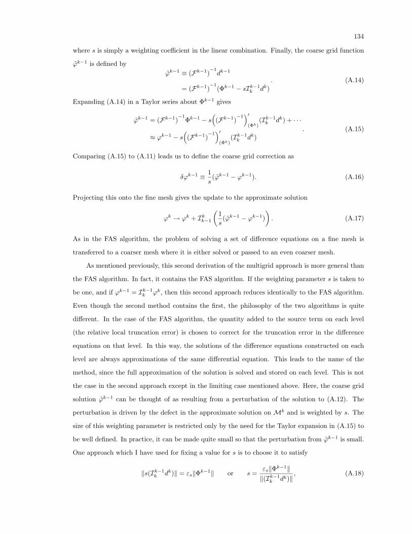
134

where s is simply a weighting coefficient in the linear combination. Finally, the coarse grid function

ϕk−1 is defined byϕk−1 ≡ (Fk−1)

−1dk−1

= (Fk−1)−1

(Φk−1 − sIk−1k dk)

. (A.14)

Expanding (A.14) in a Taylor series about Φk−1 gives

ϕk−1 = (Fk−1)−1

Φk−1 − s(

(Fk−1)−1)′

(Φk)(Ik−1k dk) + · · ·

≈ ϕk−1 − s(

(Fk−1)−1)′

(Φk)(Ik−1k dk)

. (A.15)

Comparing (A.15) to (A.11) leads us to define the coarse grid correction as

δϕk−1 ≡ 1s

(ϕk−1 − ϕk−1). (A.16)

Projecting this onto the fine mesh gives the update to the approximate solution

ϕk → ϕk + Ikk−1

(1s

(ϕk−1 − ϕk−1)). (A.17)

As in the FAS algorithm, the problem of solving a set of difference equations on a fine mesh is

transferred to a coarser mesh where it is either solved or passed to an even coarser mesh.

As mentioned previously, this second derivation of the multigrid approach is more general than

the FAS algorithm. In fact, it contains the FAS algorithm. If the weighting parameter s is taken to

be one, and if ϕk−1 = Ik−1k ϕk, then this second approach reduces identically to the FAS algorithm.

Even though the second method contains the first, the philosophy of the two algorithms is quite

different. In the case of the FAS algorithm, the quantity added to the source term on each level

(the relative local truncation error) is chosen to correct for the truncation error in the difference

equations on that level. In this way, the solutions of the difference equations constructed on each

level are always approximations of the same differential equation. This leads to the name of the

method, since the full approximation of the solution is solved and stored on each level. This is not

the case in the second approach except in the limiting case mentioned above. Here, the coarse grid

solution ϕk−1 can be thought of as resulting from a perturbation of the solution to (A.12). The

perturbation is driven by the defect in the approximate solution on Mk and is weighted by s. The

size of this weighting parameter is restricted only by the need for the Taylor expansion in (A.15) to

be well defined. In practice, it can be made quite small so that the perturbation from ϕk−1 is small.

One approach which I have used for fixing a value for s is to choose it to satisfy

‖s(Ik−1k dk)‖ = εs‖Φk−1‖ or s =

εs‖Φk−1‖‖(Ik−1

k dk)‖, (A.18)

135

where ‖ • ‖ is some appropriate vector norm and εs is an “adaptive scaling” parameter.

Appendix B contains the results for the solutions to the one-hole Hamiltonian constraint de-

scribed in Chapter 8. These solutions were obtained from a multigrid code based on the approach

outlined above. (For a detailed description of the construction of a multigrid code, see Brandt [1977],

[1982] and Choptuik [1982].) The solutions to the model problem were obtained using the FAS limit

of the code. The solutions to the physical problem of a hole with linear or angular momentum were

obtained both in the FAS limit and using adaptive scaling as described above, where εs = 0.1.

Appendix B: Numerical Solutions of the One-HoleHamiltonian Constraint

This appendix contains the most important details from the numerical solutions of the one-

hole Hamiltonian constraint described in Chapter 8. The code which produced these results was a

multigrid code based on the ideas outlined in Appendix A. In all cases, the solutions were found on

a multigrid hierarchy consisting of seven separate grids or meshes. The coarsest mesh, labeled level

zero, was discretized into 16 radial zones and six angular zones. This discretization was doubled for

each finer mesh and the finest mesh on level six was discretized into 1024 radial zones and 384 angular

zones. The outer boundary on which the approximate outer boundary condition was specified was

placed at x = 10 which places it at ∼ 22, 000 radii in the conformal space.

Seven sets of output are listed below. To gauge the accuracy of the code, the first set of outputs

lists the results from the numerical solution of the model problem described in Chapter 8. The

total energy and minimal surface mass were computed for nine separate values of the “momentum”

parameter. The values of these quantities are listed for each multigrid level and the analytic solution

is listed at the bottom of each table. Also listed for each level are two values for the L1 norm of the

relative error in the conformal factor. Since the solution is known analytically, the exact L1 error

is given as well as an estimated error for level ` computed by comparing the result on level ` with

that on level `− 1. The code was configured to solve the difference equations using the FAS limit of

the code described in Appendix A.

The next three sets of output tables contain, respectively, the results for a hole with linear

momentum based on an extrinsic curvature obeying the isometry condition with a plus sign, a

hole with linear momentum based on an extrinsic curvature obeying the isometry condition with a

minus sign, and a hole with angular momentum based on an extrinsic curvature obeying the isometry

condition with a minus sign. The code was configured to solve the difference equations using adaptive

scaling as described in Appendix A. The adaptive scaling parameter was set at εs = 0.1. The final

three sets of output tables consist of the same solution set as the previous three except that the code

was configured to solve the difference equations using the FAS limit of the code.

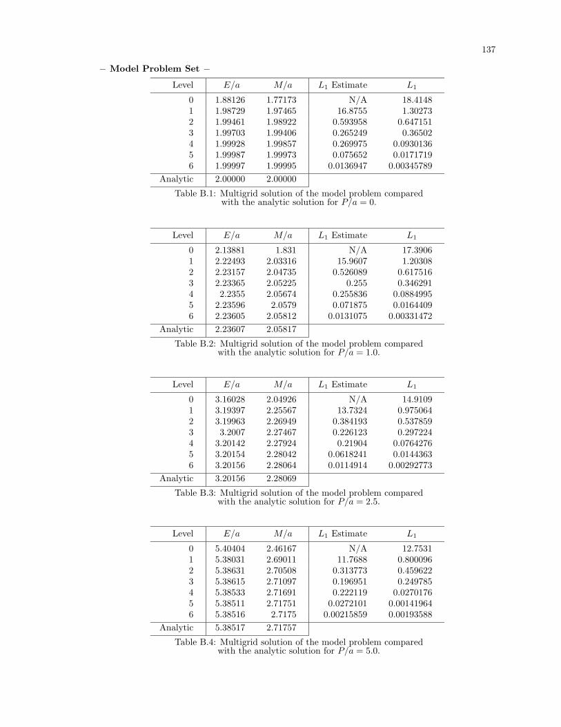
137

− Model Problem Set −

Level E/a M/a L1 Estimate L1

0 1.88126 1.77173 N/A 18.41481 1.98729 1.97465 16.8755 1.302732 1.99461 1.98922 0.593958 0.6471513 1.99703 1.99406 0.265249 0.365024 1.99928 1.99857 0.269975 0.09301365 1.99987 1.99973 0.075652 0.01717196 1.99997 1.99995 0.0136947 0.00345789

Analytic 2.00000 2.00000

Table B.1: Multigrid solution of the model problem comparedwith the analytic solution for P/a = 0.

Level E/a M/a L1 Estimate L1

0 2.13881 1.831 N/A 17.39061 2.22493 2.03316 15.9607 1.203082 2.23157 2.04735 0.526089 0.6175163 2.23365 2.05225 0.255 0.3462914 2.2355 2.05674 0.255836 0.08849955 2.23596 2.0579 0.071875 0.01644096 2.23605 2.05812 0.0131075 0.00331472

Analytic 2.23607 2.05817

Table B.2: Multigrid solution of the model problem comparedwith the analytic solution for P/a = 1.0.

Level E/a M/a L1 Estimate L1

0 3.16028 2.04926 N/A 14.91091 3.19397 2.25567 13.7324 0.9750642 3.19963 2.26949 0.384193 0.5378593 3.2007 2.27467 0.226123 0.2972244 3.20142 2.27924 0.21904 0.07642765 3.20154 2.28042 0.0618241 0.01443636 3.20156 2.28064 0.0114914 0.00292773

Analytic 3.20156 2.28069

Table B.3: Multigrid solution of the model problem comparedwith the analytic solution for P/a = 2.5.

Level E/a M/a L1 Estimate L1

0 5.40404 2.46167 N/A 12.75311 5.38031 2.69011 11.7688 0.8000962 5.38631 2.70508 0.313773 0.4596223 5.38615 2.71097 0.196951 0.2497854 5.38533 2.71691 0.222119 0.02701765 5.38511 2.71751 0.0272101 0.001419646 5.38516 2.7175 0.00215859 0.00193588

Analytic 5.38517 2.71757

Table B.4: Multigrid solution of the model problem comparedwith the analytic solution for P/a = 5.0.

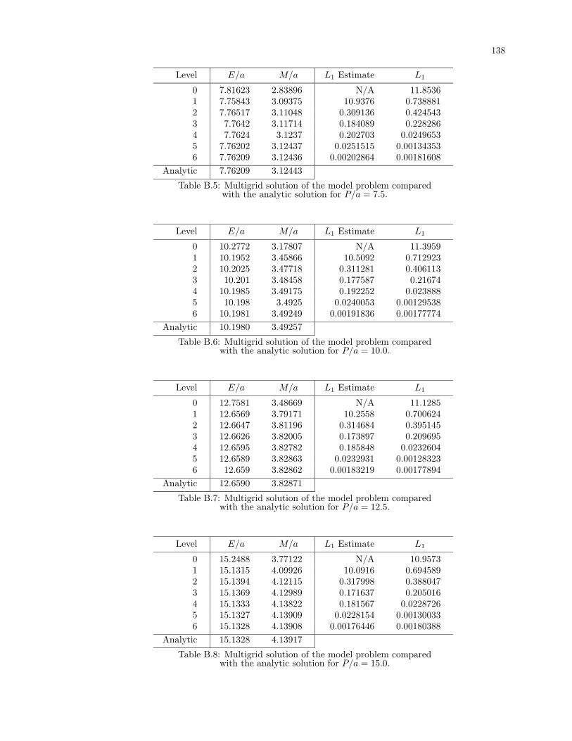
138

Level E/a M/a L1 Estimate L1

0 7.81623 2.83896 N/A 11.85361 7.75843 3.09375 10.9376 0.7388812 7.76517 3.11048 0.309136 0.4245433 7.7642 3.11714 0.184089 0.2282864 7.7624 3.1237 0.202703 0.02496535 7.76202 3.12437 0.0251515 0.001343536 7.76209 3.12436 0.00202864 0.00181608

Analytic 7.76209 3.12443

Table B.5: Multigrid solution of the model problem comparedwith the analytic solution for P/a = 7.5.

Level E/a M/a L1 Estimate L1

0 10.2772 3.17807 N/A 11.39591 10.1952 3.45866 10.5092 0.7129232 10.2025 3.47718 0.311281 0.4061133 10.201 3.48458 0.177587 0.216744 10.1985 3.49175 0.192252 0.0238885 10.198 3.4925 0.0240053 0.001295386 10.1981 3.49249 0.00191836 0.00177774

Analytic 10.1980 3.49257

Table B.6: Multigrid solution of the model problem comparedwith the analytic solution for P/a = 10.0.

Level E/a M/a L1 Estimate L1

0 12.7581 3.48669 N/A 11.12851 12.6569 3.79171 10.2558 0.7006242 12.6647 3.81196 0.314684 0.3951453 12.6626 3.82005 0.173897 0.2096954 12.6595 3.82782 0.185848 0.02326045 12.6589 3.82863 0.0232931 0.001283236 12.659 3.82862 0.00183219 0.00177894

Analytic 12.6590 3.82871

Table B.7: Multigrid solution of the model problem comparedwith the analytic solution for P/a = 12.5.

Level E/a M/a L1 Estimate L1

0 15.2488 3.77122 N/A 10.95731 15.1315 4.09926 10.0916 0.6945892 15.1394 4.12115 0.317998 0.3880473 15.1369 4.12989 0.171637 0.2050164 15.1333 4.13822 0.181567 0.02287265 15.1327 4.13909 0.0228154 0.001300336 15.1328 4.13908 0.00176446 0.00180388

Analytic 15.1328 4.13917

Table B.8: Multigrid solution of the model problem comparedwith the analytic solution for P/a = 15.0.

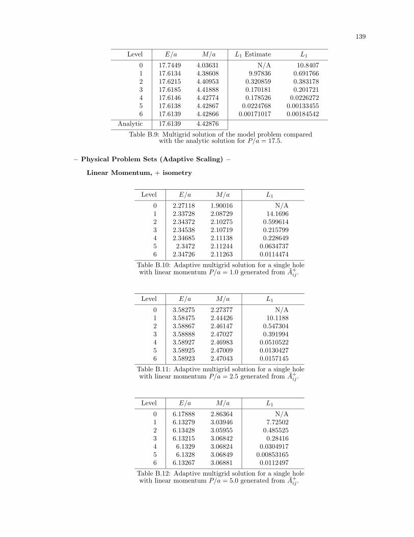
139

Level E/a M/a L1 Estimate L1

0 17.7449 4.03631 N/A 10.84071 17.6134 4.38608 9.97836 0.6917662 17.6215 4.40953 0.320859 0.3831783 17.6185 4.41888 0.170181 0.2017214 17.6146 4.42774 0.178526 0.02262725 17.6138 4.42867 0.0224768 0.001334556 17.6139 4.42866 0.00171017 0.00184542

Analytic 17.6139 4.42876

Table B.9: Multigrid solution of the model problem comparedwith the analytic solution for P/a = 17.5.

− Physical Problem Sets (Adaptive Scaling) −

Linear Momentum, + isometry

Level E/a M/a L1

0 2.27118 1.90016 N/A1 2.33728 2.08729 14.16962 2.34372 2.10275 0.5996143 2.34538 2.10719 0.2157994 2.34685 2.11138 0.2286495 2.3472 2.11244 0.06347376 2.34726 2.11263 0.0114474

Table B.10: Adaptive multigrid solution for a single holewith linear momentum P/a = 1.0 generated from A+

ij .

Level E/a M/a L1

0 3.58275 2.27377 N/A1 3.58475 2.44426 10.11882 3.58867 2.46147 0.5473043 3.58888 2.47027 0.3919944 3.58927 2.46983 0.05105225 3.58925 2.47009 0.01304276 3.58923 2.47043 0.0157145

Table B.11: Adaptive multigrid solution for a single holewith linear momentum P/a = 2.5 generated from A+

ij .

Level E/a M/a L1

0 6.17888 2.86364 N/A1 6.13279 3.03946 7.725022 6.13428 3.05955 0.4855253 6.13215 3.06842 0.284164 6.1329 3.06824 0.03049175 6.1328 3.06849 0.008531656 6.13267 3.06881 0.0112497

Table B.12: Adaptive multigrid solution for a single holewith linear momentum P/a = 5.0 generated from A+

ij .

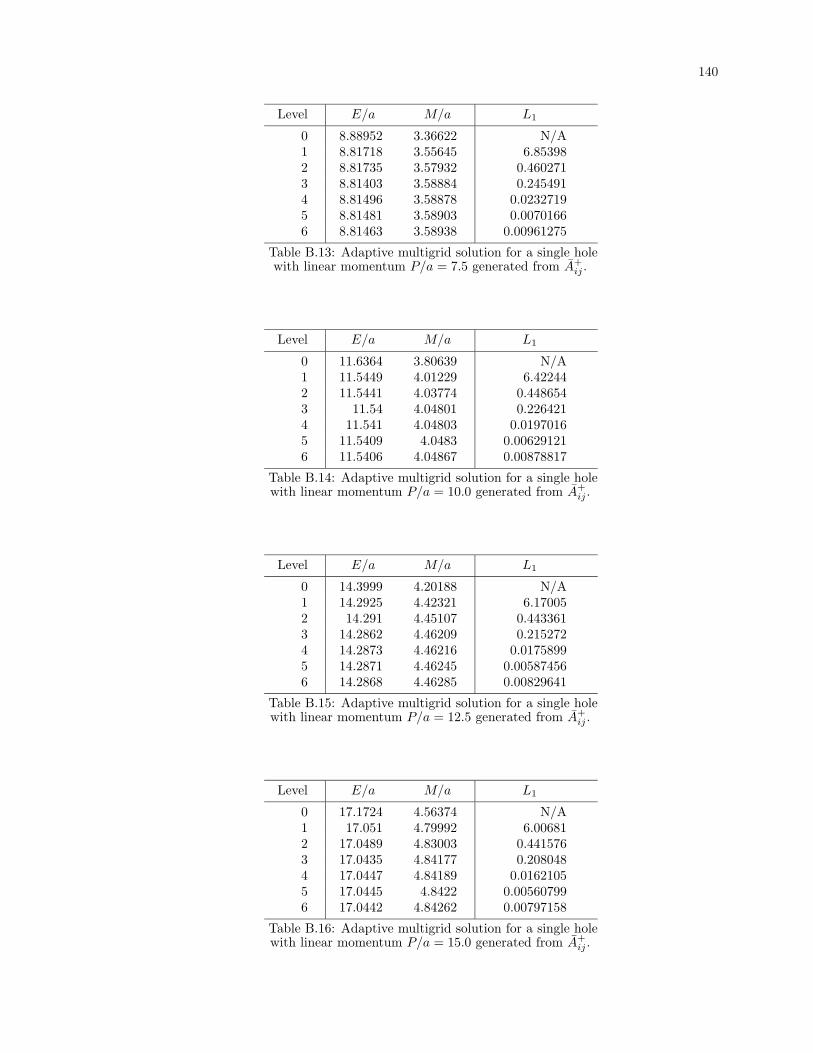
140

Level E/a M/a L1

0 8.88952 3.36622 N/A1 8.81718 3.55645 6.853982 8.81735 3.57932 0.4602713 8.81403 3.58884 0.2454914 8.81496 3.58878 0.02327195 8.81481 3.58903 0.00701666 8.81463 3.58938 0.00961275

Table B.13: Adaptive multigrid solution for a single holewith linear momentum P/a = 7.5 generated from A+

ij .

Level E/a M/a L1

0 11.6364 3.80639 N/A1 11.5449 4.01229 6.422442 11.5441 4.03774 0.4486543 11.54 4.04801 0.2264214 11.541 4.04803 0.01970165 11.5409 4.0483 0.006291216 11.5406 4.04867 0.00878817

Table B.14: Adaptive multigrid solution for a single holewith linear momentum P/a = 10.0 generated from A+

ij .

Level E/a M/a L1

0 14.3999 4.20188 N/A1 14.2925 4.42321 6.170052 14.291 4.45107 0.4433613 14.2862 4.46209 0.2152724 14.2873 4.46216 0.01758995 14.2871 4.46245 0.005874566 14.2868 4.46285 0.00829641

Table B.15: Adaptive multigrid solution for a single holewith linear momentum P/a = 12.5 generated from A+

ij .

Level E/a M/a L1

0 17.1724 4.56374 N/A1 17.051 4.79992 6.006812 17.0489 4.83003 0.4415763 17.0435 4.84177 0.2080484 17.0447 4.84189 0.01621055 17.0445 4.8422 0.005607996 17.0442 4.84262 0.00797158

Table B.16: Adaptive multigrid solution for a single holewith linear momentum P/a = 15.0 generated from A+

ij .

141

Level E/a M/a L1

0 19.9505 4.8992 N/A1 19.8164 5.14958 5.893862 19.8137 5.18181 0.4415173 19.8078 5.19424 0.2030334 19.8091 5.19441 0.01534035 19.8088 5.19473 0.005424866 19.8085 5.19517 0.00774191

Table B.17: Adaptive multigrid solution for a single holewith linear momentum P/a = 17.5 generated from A+

ij .

Linear Momentum, − isometry

Level E/a M/a L1

0 2.24839 1.88262 N/A1 2.31919 2.07431 14.70242 2.32571 2.08941 0.5759973 2.32747 2.09399 0.2275574 2.32902 2.09827 0.2363935 2.3294 2.09936 0.0658336 2.32947 2.09956 0.0119361

Table B.18: Adaptive multigrid solution for a single holewith linear momentum P/a = 1.0 generated from A−ij .

Level E/a M/a L1

0 3.53242 2.22443 N/A1 3.5393 2.40394 11.0112 3.54386 2.42068 0.5247563 3.54444 2.42499 0.1630164 3.54464 2.429 0.1754165 3.54461 2.42999 0.04803086 3.5446 2.43017 0.00874135

Table B.19: Adaptive multigrid solution for a single holewith linear momentum P/a = 2.5 generated from A−ij .

Level E/a M/a L1

0 6.12118 2.78323 N/A1 6.0766 2.97079 8.628982 6.07923 2.99066 0.4814173 6.07897 2.99522 0.1226334 6.07803 2.99938 0.1340045 6.07767 3.00037 0.03591936 6.0776 3.00055 0.0065615

Table B.20: Adaptive multigrid solution for a single holewith linear momentum P/a = 5.0 generated from A−ij .

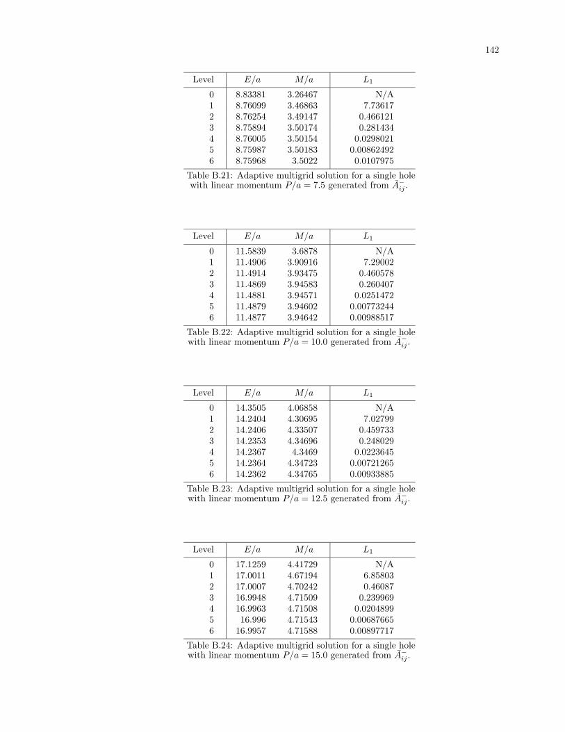
142

Level E/a M/a L1

0 8.83381 3.26467 N/A1 8.76099 3.46863 7.736172 8.76254 3.49147 0.4661213 8.75894 3.50174 0.2814344 8.76005 3.50154 0.02980215 8.75987 3.50183 0.008624926 8.75968 3.5022 0.0107975

Table B.21: Adaptive multigrid solution for a single holewith linear momentum P/a = 7.5 generated from A−ij .

Level E/a M/a L1

0 11.5839 3.6878 N/A1 11.4906 3.90916 7.290022 11.4914 3.93475 0.4605783 11.4869 3.94583 0.2604074 11.4881 3.94571 0.02514725 11.4879 3.94602 0.007732446 11.4877 3.94642 0.00988517

Table B.22: Adaptive multigrid solution for a single holewith linear momentum P/a = 10.0 generated from A−ij .

Level E/a M/a L1

0 14.3505 4.06858 N/A1 14.2404 4.30695 7.027992 14.2406 4.33507 0.4597333 14.2353 4.34696 0.2480294 14.2367 4.3469 0.02236455 14.2364 4.34723 0.007212656 14.2362 4.34765 0.00933885

Table B.23: Adaptive multigrid solution for a single holewith linear momentum P/a = 12.5 generated from A−ij .

Level E/a M/a L1

0 17.1259 4.41729 N/A1 17.0011 4.67194 6.858032 17.0007 4.70242 0.460873 16.9948 4.71509 0.2399694 16.9963 4.71508 0.02048995 16.996 4.71543 0.006876656 16.9957 4.71588 0.00897717

Table B.24: Adaptive multigrid solution for a single holewith linear momentum P/a = 15.0 generated from A−ij .

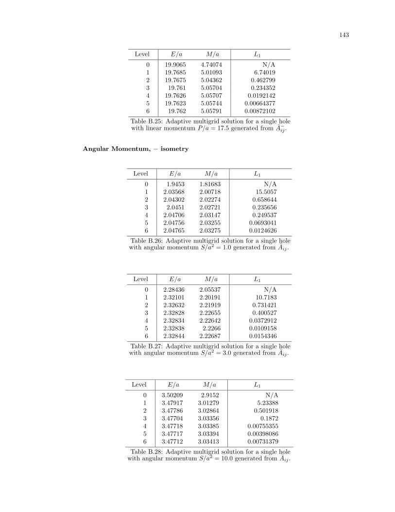
143

Level E/a M/a L1

0 19.9065 4.74074 N/A1 19.7685 5.01093 6.740192 19.7675 5.04362 0.4627993 19.761 5.05704 0.2343524 19.7626 5.05707 0.01921425 19.7623 5.05744 0.006643776 19.762 5.05791 0.00872102

Table B.25: Adaptive multigrid solution for a single holewith linear momentum P/a = 17.5 generated from A−ij .

Angular Momentum, − isometry

Level E/a M/a L1

0 1.9453 1.81683 N/A1 2.03568 2.00718 15.50572 2.04302 2.02274 0.6586443 2.0451 2.02721 0.2356564 2.04706 2.03147 0.2495375 2.04756 2.03255 0.06930416 2.04765 2.03275 0.0124626

Table B.26: Adaptive multigrid solution for a single holewith angular momentum S/a2 = 1.0 generated from Aij .

Level E/a M/a L1

0 2.28436 2.05537 N/A1 2.32101 2.20191 10.71832 2.32632 2.21919 0.7314213 2.32828 2.22655 0.4005274 2.32834 2.22642 0.03729125 2.32838 2.2266 0.01091586 2.32844 2.22687 0.0154346

Table B.27: Adaptive multigrid solution for a single holewith angular momentum S/a2 = 3.0 generated from Aij .

Level E/a M/a L1

0 3.50209 2.9152 N/A1 3.47917 3.01279 5.233882 3.47786 3.02864 0.5019183 3.47704 3.03356 0.18724 3.47718 3.03385 0.007553555 3.47717 3.03394 0.003980866 3.47712 3.03413 0.00731379

Table B.28: Adaptive multigrid solution for a single holewith angular momentum S/a2 = 10.0 generated from Aij .

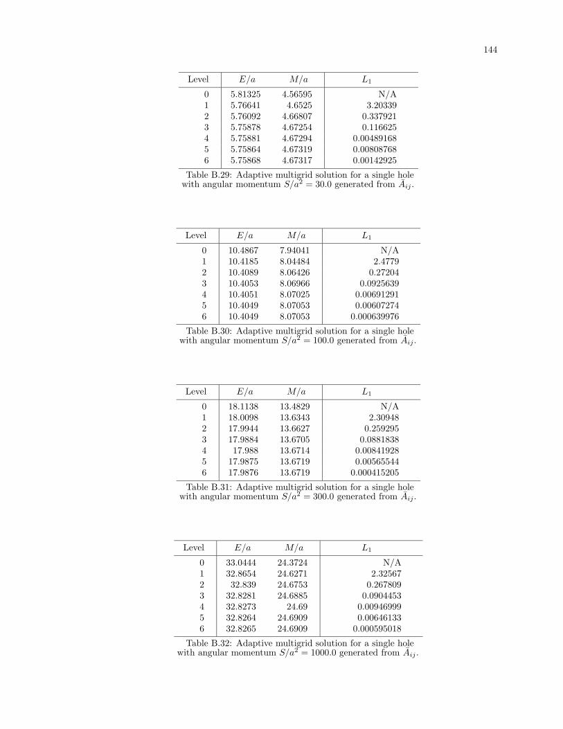
144

Level E/a M/a L1

0 5.81325 4.56595 N/A1 5.76641 4.6525 3.203392 5.76092 4.66807 0.3379213 5.75878 4.67254 0.1166254 5.75881 4.67294 0.004891685 5.75864 4.67319 0.008087686 5.75868 4.67317 0.00142925

Table B.29: Adaptive multigrid solution for a single holewith angular momentum S/a2 = 30.0 generated from Aij .

Level E/a M/a L1

0 10.4867 7.94041 N/A1 10.4185 8.04484 2.47792 10.4089 8.06426 0.272043 10.4053 8.06966 0.09256394 10.4051 8.07025 0.006912915 10.4049 8.07053 0.006072746 10.4049 8.07053 0.000639976

Table B.30: Adaptive multigrid solution for a single holewith angular momentum S/a2 = 100.0 generated from Aij .

Level E/a M/a L1

0 18.1138 13.4829 N/A1 18.0098 13.6343 2.309482 17.9944 13.6627 0.2592953 17.9884 13.6705 0.08818384 17.988 13.6714 0.008419285 17.9875 13.6719 0.005655446 17.9876 13.6719 0.000415205

Table B.31: Adaptive multigrid solution for a single holewith angular momentum S/a2 = 300.0 generated from Aij .

Level E/a M/a L1

0 33.0444 24.3724 N/A1 32.8654 24.6271 2.325672 32.839 24.6753 0.2678093 32.8281 24.6885 0.09044534 32.8273 24.69 0.009469995 32.8264 24.6909 0.006461336 32.8265 24.6909 0.000595018

Table B.32: Adaptive multigrid solution for a single holewith angular momentum S/a2 = 1000.0 generated from Aij .

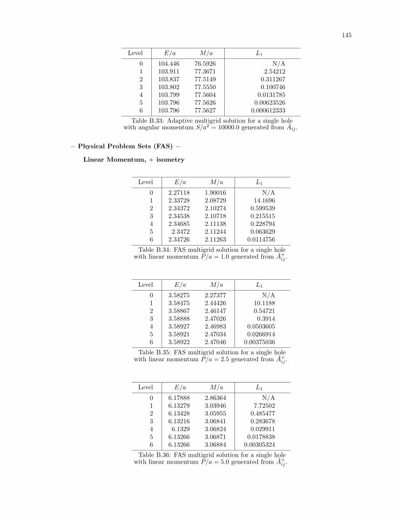
145

Level E/a M/a L1

0 104.446 76.5926 N/A1 103.911 77.3671 2.542122 103.837 77.5149 0.3112673 103.802 77.5550 0.1007464 103.799 77.5604 0.01317855 103.796 77.5626 0.006235266 103.796 77.5627 0.000612333

Table B.33: Adaptive multigrid solution for a single holewith angular momentum S/a2 = 10000.0 generated from Aij .

− Physical Problem Sets (FAS) −

Linear Momentum, + isometry

Level E/a M/a L1

0 2.27118 1.90016 N/A1 2.33728 2.08729 14.16962 2.34372 2.10274 0.5995393 2.34538 2.10718 0.2155154 2.34685 2.11138 0.2287945 2.3472 2.11244 0.0636296 2.34726 2.11263 0.0114756

Table B.34: FAS multigrid solution for a single holewith linear momentum P/a = 1.0 generated from A+

ij .

Level E/a M/a L1

0 3.58275 2.27377 N/A1 3.58475 2.44426 10.11882 3.58867 2.46147 0.547213 3.58888 2.47026 0.39144 3.58927 2.46983 0.05036055 3.58921 2.47034 0.02669146 3.58922 2.47046 0.00375036

Table B.35: FAS multigrid solution for a single holewith linear momentum P/a = 2.5 generated from A+

ij .

Level E/a M/a L1

0 6.17888 2.86364 N/A1 6.13279 3.03946 7.725022 6.13428 3.05955 0.4854773 6.13216 3.06841 0.2836784 6.1329 3.06824 0.0299115 6.13266 3.06871 0.01788386 6.13266 3.06884 0.00305324

Table B.36: FAS multigrid solution for a single holewith linear momentum P/a = 5.0 generated from A+

ij .

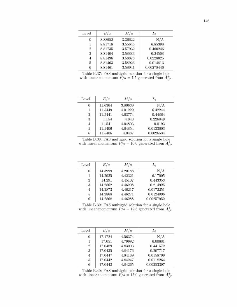
146

Level E/a M/a L1

0 8.88952 3.36622 N/A1 8.81718 3.55645 6.853982 8.81735 3.57932 0.4602463 8.81404 3.58883 0.245084 8.81496 3.58878 0.02280255 8.81463 3.58926 0.0148136 8.81461 3.58941 0.00278446

Table B.37: FAS multigrid solution for a single holewith linear momentum P/a = 7.5 generated from A+

ij .

Level E/a M/a L1

0 11.6364 3.80639 N/A1 11.5449 4.01229 6.422442 11.5441 4.03774 0.448643 11.54 4.048 0.2260494 11.541 4.04803 0.01935 11.5406 4.04854 0.01330036 11.5406 4.0487 0.0026534

Table B.38: FAS multigrid solution for a single holewith linear momentum P/a = 10.0 generated from A+

ij .

Level E/a M/a L1

0 14.3999 4.20188 N/A1 14.2925 4.42321 6.170052 14.291 4.45107 0.4433533 14.2862 4.46208 0.2149254 14.2873 4.46217 0.01722515 14.2868 4.46271 0.01240966 14.2868 4.46288 0.00257952

Table B.39: FAS multigrid solution for a single holewith linear momentum P/a = 12.5 generated from A+

ij .

Level E/a M/a L1

0 17.1724 4.56374 N/A1 17.051 4.79992 6.006812 17.0489 4.83003 0.4415723 17.0435 4.84176 0.2077174 17.0447 4.84189 0.01587995 17.0442 4.84247 0.01182646 17.0442 4.84265 0.00253397

Table B.40: FAS multigrid solution for a single holewith linear momentum P/a = 15.0 generated from A+

ij .

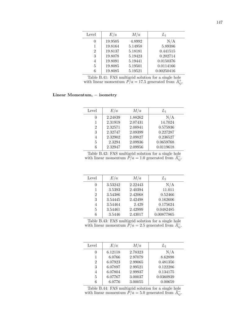
147

Level E/a M/a L1

0 19.9505 4.8992 N/A1 19.8164 5.14958 5.893862 19.8137 5.18181 0.4415153 19.8078 5.19423 0.2027144 19.8091 5.19441 0.01503765 19.8085 5.19501 0.01141666 19.8085 5.19521 0.00250416

Table B.41: FAS multigrid solution for a single holewith linear momentum P/a = 17.5 generated from A+

ij .

Linear Momentum, − isometry

Level E/a M/a L1

0 2.24839 1.88262 N/A1 2.31919 2.07431 14.70242 2.32571 2.08941 0.5759363 2.32747 2.09399 0.2272874 2.32902 2.09827 0.2365275 2.3294 2.09936 0.06597686 2.32947 2.09956 0.0119618

Table B.42: FAS multigrid solution for a single holewith linear momentum P/a = 1.0 generated from A−ij .

Level E/a M/a L1

0 3.53242 2.22443 N/A1 3.5393 2.40394 11.0112 3.54386 2.42068 0.524663 3.54445 2.42498 0.1626064 3.54464 2.429 0.1756245 3.54461 2.42999 0.04824856 3.5446 2.43017 0.00877865

Table B.43: FAS multigrid solution for a single holewith linear momentum P/a = 2.5 generated from A−ij .

Level E/a M/a L1

0 6.12118 2.78323 N/A1 6.0766 2.97079 8.628982 6.07923 2.99065 0.4813563 6.07897 2.99521 0.1222864 6.07804 2.99937 0.1341755 6.07767 3.00037 0.03609396 6.0776 3.00055 0.00659

Table B.44: FAS multigrid solution for a single holewith linear momentum P/a = 5.0 generated from A−ij .

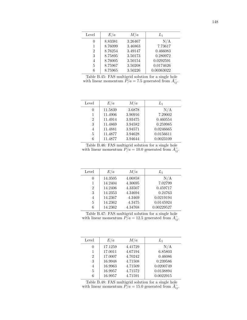
148

Level E/a M/a L1

0 8.83381 3.26467 N/A1 8.76099 3.46863 7.736172 8.76254 3.49147 0.4660833 8.75895 3.50173 0.2809724 8.76005 3.50154 0.02925915 8.75967 3.50208 0.01746266 8.75965 3.50226 0.00363022

Table B.45: FAS multigrid solution for a single holewith linear momentum P/a = 7.5 generated from A−ij .

Level E/a M/a L1

0 11.5839 3.6878 N/A1 11.4906 3.90916 7.290022 11.4914 3.93475 0.4605543 11.4869 3.94582 0.2599854 11.4881 3.94571 0.02466655 11.4877 3.94628 0.01566116 11.4877 3.94644 0.0023109

Table B.46: FAS multigrid solution for a single holewith linear momentum P/a = 10.0 generated from A−ij .

Level E/a M/a L1

0 14.3505 4.06858 N/A1 14.2404 4.30695 7.027992 14.2406 4.33507 0.4597173 14.2353 4.34694 0.247634 14.2367 4.3469 0.02191945 14.2362 4.3475 0.01459246 14.2362 4.34768 0.00229527

Table B.47: FAS multigrid solution for a single holewith linear momentum P/a = 12.5 generated from A−ij .

Level E/a M/a L1

0 17.1259 4.41729 N/A1 17.0011 4.67194 6.858032 17.0007 4.70242 0.460863 16.9948 4.71508 0.2395864 16.9963 4.71509 0.02007495 16.9957 4.71572 0.01388946 16.9957 4.71591 0.0022915

Table B.48: FAS multigrid solution for a single holewith linear momentum P/a = 15.0 generated from A−ij .

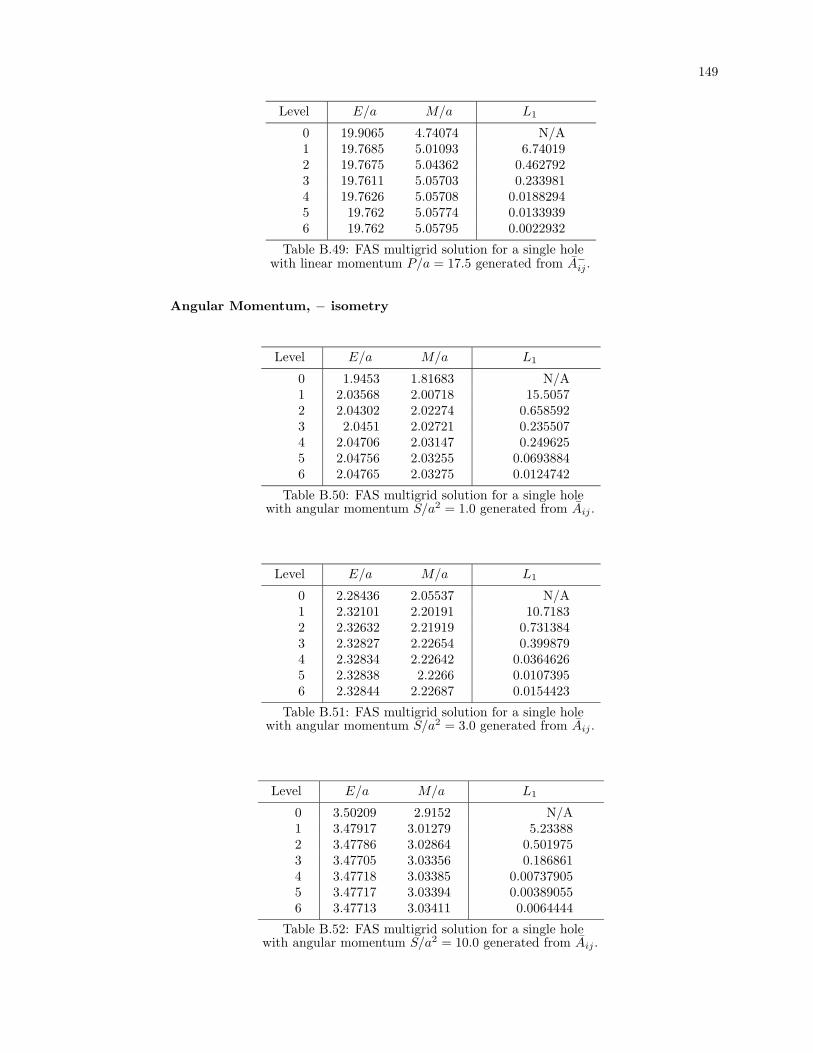
149

Level E/a M/a L1

0 19.9065 4.74074 N/A1 19.7685 5.01093 6.740192 19.7675 5.04362 0.4627923 19.7611 5.05703 0.2339814 19.7626 5.05708 0.01882945 19.762 5.05774 0.01339396 19.762 5.05795 0.0022932

Table B.49: FAS multigrid solution for a single holewith linear momentum P/a = 17.5 generated from A−ij .

Angular Momentum, − isometry

Level E/a M/a L1

0 1.9453 1.81683 N/A1 2.03568 2.00718 15.50572 2.04302 2.02274 0.6585923 2.0451 2.02721 0.2355074 2.04706 2.03147 0.2496255 2.04756 2.03255 0.06938846 2.04765 2.03275 0.0124742

Table B.50: FAS multigrid solution for a single holewith angular momentum S/a2 = 1.0 generated from Aij .

Level E/a M/a L1

0 2.28436 2.05537 N/A1 2.32101 2.20191 10.71832 2.32632 2.21919 0.7313843 2.32827 2.22654 0.3998794 2.32834 2.22642 0.03646265 2.32838 2.2266 0.01073956 2.32844 2.22687 0.0154423

Table B.51: FAS multigrid solution for a single holewith angular momentum S/a2 = 3.0 generated from Aij .

Level E/a M/a L1

0 3.50209 2.9152 N/A1 3.47917 3.01279 5.233882 3.47786 3.02864 0.5019753 3.47705 3.03356 0.1868614 3.47718 3.03385 0.007379055 3.47717 3.03394 0.003890556 3.47713 3.03411 0.0064444

Table B.52: FAS multigrid solution for a single holewith angular momentum S/a2 = 10.0 generated from Aij .

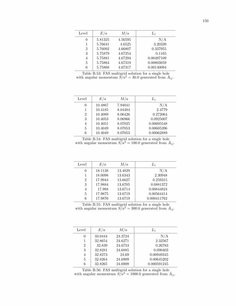
150

Level E/a M/a L1

0 5.81325 4.56595 N/A1 5.76641 4.6525 3.203392 5.76092 4.66807 0.3379553 5.75879 4.67254 0.11654 5.75881 4.67294 0.004971095 5.75864 4.67319 0.008038596 5.75868 4.67317 0.00140094

Table B.53: FAS multigrid solution for a single holewith angular momentum S/a2 = 30.0 generated from Aij .

Level E/a M/a L1

0 10.4867 7.94041 N/A1 10.4185 8.04484 2.47792 10.4089 8.06426 0.2720643 10.4053 8.06966 0.09250074 10.4051 8.07025 0.006955485 10.4049 8.07053 0.006053966 10.4049 8.07053 0.00062889

Table B.54: FAS multigrid solution for a single holewith angular momentum S/a2 = 100.0 generated from Aij .

Level E/a M/a L1

0 18.1138 13.4829 N/A1 18.0098 13.6343 2.309482 17.9944 13.6627 0.2593153 17.9884 13.6705 0.08813724 17.988 13.6714 0.008448245 17.9875 13.6719 0.005644146 17.9876 13.6719 0.000411762

Table B.55: FAS multigrid solution for a single holewith angular momentum S/a2 = 300.0 generated from Aij .

Level E/a M/a L1

0 33.0444 24.3724 N/A1 32.8654 24.6271 2.325672 32.839 24.6753 0.267833 32.8281 24.6885 0.0904034 32.8273 24.69 0.009493455 32.8264 24.6909 0.006452026 32.8265 24.6909 0.000591245

Table B.56: FAS multigrid solution for a single holewith angular momentum S/a2 = 1000.0 generated from Aij .

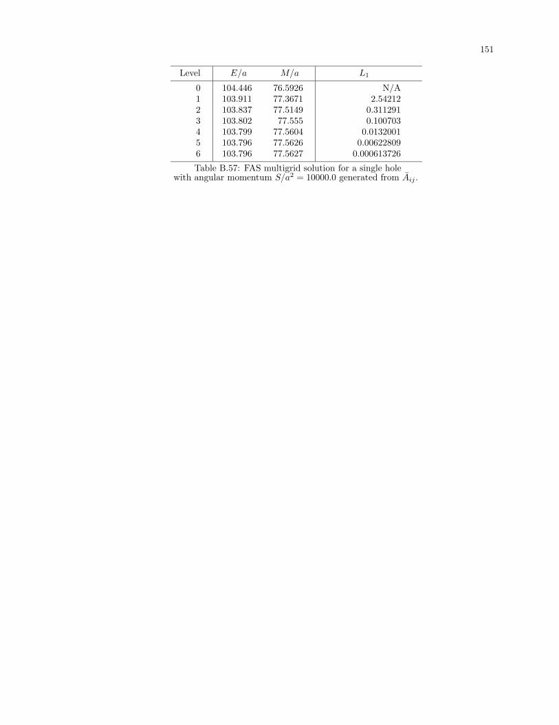
151

Level E/a M/a L1

0 104.446 76.5926 N/A1 103.911 77.3671 2.542122 103.837 77.5149 0.3112913 103.802 77.555 0.1007034 103.799 77.5604 0.01320015 103.796 77.5626 0.006228096 103.796 77.5627 0.000613726

Table B.57: FAS multigrid solution for a single holewith angular momentum S/a2 = 10000.0 generated from Aij .

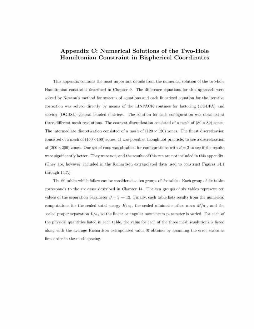
Appendix C: Numerical Solutions of the Two-HoleHamiltonian Constraint in Bispherical Coordinates

This appendix contains the most important details from the numerical solution of the two-hole

Hamiltonian constraint described in Chapter 9. The difference equations for this approach were

solved by Newton’s method for systems of equations and each linearized equation for the iterative

correction was solved directly by means of the LINPACK routines for factoring (DGBFA) and

solving (DGBSL) general banded matrices. The solution for each configuration was obtained at

three different mesh resolutions. The coarsest discretization consisted of a mesh of (80× 80) zones.

The intermediate discretization consisted of a mesh of (120 × 120) zones. The finest discretization

consisted of a mesh of (160×160) zones. It was possible, though not practicle, to use a discretization

of (200× 200) zones. One set of runs was obtained for configurations with β = 3 to see if the results

were significantly better. They were not, and the results of this run are not included in this appendix.

(They are, however, included in the Richardson extrapolated data used to construct Figures 14.1

through 14.7.)

The 60 tables which follow can be considered as ten groups of six tables. Each group of six tables

corresponds to the six cases described in Chapter 14. The ten groups of six tables represent ten

values of the separation parameter β = 3→ 12. Finally, each table lists results from the numerical

computations for the scaled total energy E/a1, the scaled minimal surface mass M/a1, and the

scaled proper separation L/a1 as the linear or angular momentum parameter is varied. For each of

the physical quantities listed in each table, the value for each of the three mesh resolutions is listed

along with the average Richardson extrapolated value < obtaind by assuming the error scales as

first order in the mesh spacing.

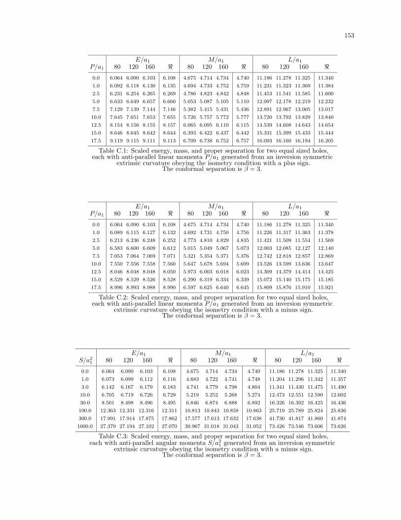
153

E/a1 M/a1 L/a1

P/a1 80 120 160 < 80 120 160 < 80 120 160 <0.0 6.064 6.090 6.103 6.108 4.675 4.714 4.734 4.740 11.186 11.278 11.325 11.340

1.0 6.092 6.118 6.130 6.135 4.694 4.733 4.752 4.759 11.231 11.323 11.369 11.384

2.5 6.231 6.254 6.265 6.269 4.786 4.823 4.842 4.848 11.453 11.541 11.585 11.600

5.0 6.633 6.649 6.657 6.660 5.053 5.087 5.105 5.110 12.097 12.178 12.219 12.232

7.5 7.129 7.139 7.144 7.146 5.382 5.415 5.431 5.436 12.891 12.967 13.005 13.017

10.0 7.645 7.651 7.653 7.655 5.726 5.757 5.772 5.777 13.720 13.792 13.829 13.840

12.5 8.154 8.156 8.155 8.157 6.065 6.095 6.110 6.115 14.539 14.608 14.643 14.654

15.0 8.646 8.645 8.642 8.644 6.393 6.422 6.437 6.442 15.331 15.399 15.433 15.444

17.5 9.119 9.115 9.111 9.113 6.709 6.738 6.752 6.757 16.093 16.160 16.194 16.205

Table C.1: Scaled energy, mass, and proper separation for two equal sized holes,each with anti-parallel linear momenta P/a1 generated from an inversion symmetric

extrinsic curvature obeying the isometry condition with a plus sign.The conformal separation is β = 3.

E/a1 M/a1 L/a1

P/a1 80 120 160 < 80 120 160 < 80 120 160 <0.0 6.064 6.090 6.103 6.108 4.675 4.714 4.734 4.740 11.186 11.278 11.325 11.340

1.0 6.089 6.115 6.127 6.132 4.692 4.731 4.750 4.756 11.226 11.317 11.363 11.378

2.5 6.213 6.236 6.248 6.252 4.773 4.810 4.829 4.835 11.421 11.509 11.554 11.569

5.0 6.583 6.600 6.609 6.612 5.015 5.049 5.067 5.073 12.003 12.085 12.127 12.140

7.5 7.053 7.064 7.069 7.071 5.321 5.354 5.371 5.376 12.742 12.818 12.857 12.869

10.0 7.550 7.556 7.558 7.560 5.647 5.678 5.694 5.699 13.526 13.599 13.636 13.647

12.5 8.046 8.048 8.048 8.050 5.973 6.003 6.018 6.023 14.309 14.379 14.414 14.425

15.0 8.529 8.529 8.526 8.528 6.290 6.319 6.334 6.339 15.072 15.140 15.175 15.185

17.5 8.996 8.993 8.988 8.990 6.597 6.625 6.640 6.645 15.809 15.876 15.910 15.921

Table C.2: Scaled energy, mass, and proper separation for two equal sized holes,each with anti-parallel linear momenta P/a1 generated from an inversion symmetric

extrinsic curvature obeying the isometry condition with a minus sign.The conformal separation is β = 3.

E/a1 M/a1 L/a1

S/a21 80 120 160 < 80 120 160 < 80 120 160 <

0.0 6.064 6.090 6.103 6.108 4.675 4.714 4.734 4.740 11.186 11.278 11.325 11.340

1.0 6.073 6.099 6.112 6.116 4.683 4.722 4.741 4.748 11.204 11.296 11.342 11.357

3.0 6.142 6.167 6.179 6.183 4.741 4.779 4.798 4.804 11.341 11.430 11.475 11.490

10.0 6.705 6.719 6.726 6.729 5.219 5.252 5.268 5.274 12.473 12.551 12.590 12.602

30.0 8.501 8.498 8.496 8.495 6.846 6.874 6.888 6.892 16.326 16.392 16.425 16.436

100.0 12.363 12.331 12.316 12.311 10.813 10.843 10.858 10.863 25.719 25.789 25.824 25.836

300.0 17.991 17.914 17.875 17.862 17.577 17.613 17.632 17.638 41.730 41.817 41.860 41.874

1000.0 27.379 27.194 27.102 27.070 30.967 31.018 31.043 31.052 73.426 73.546 73.606 73.626

Table C.3: Scaled energy, mass, and proper separation for two equal sized holes,each with anti-parallel angular momenta S/a2

1 generated from an inversion symmetricextrinsic curvature obeying the isometry condition with a minus sign.

The conformal separation is β = 3.

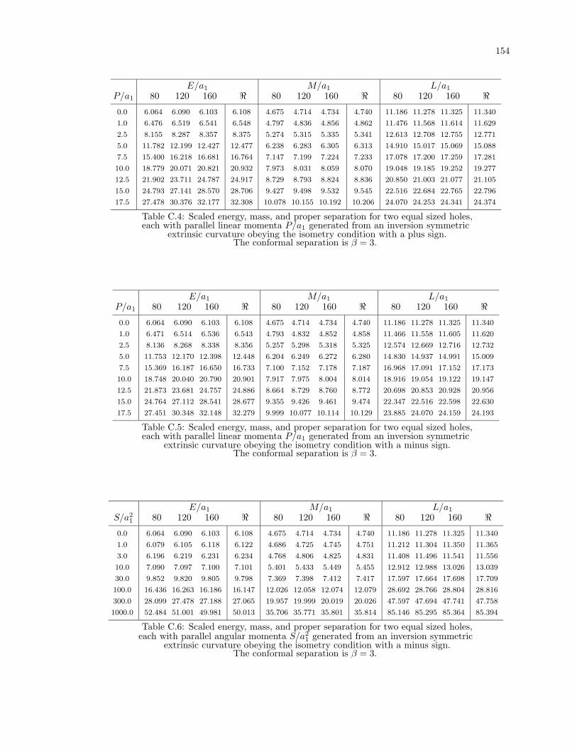
154

E/a1 M/a1 L/a1

P/a1 80 120 160 < 80 120 160 < 80 120 160 <0.0 6.064 6.090 6.103 6.108 4.675 4.714 4.734 4.740 11.186 11.278 11.325 11.340

1.0 6.476 6.519 6.541 6.548 4.797 4.836 4.856 4.862 11.476 11.568 11.614 11.629

2.5 8.155 8.287 8.357 8.375 5.274 5.315 5.335 5.341 12.613 12.708 12.755 12.771

5.0 11.782 12.199 12.427 12.477 6.238 6.283 6.305 6.313 14.910 15.017 15.069 15.088

7.5 15.400 16.218 16.681 16.764 7.147 7.199 7.224 7.233 17.078 17.200 17.259 17.281

10.0 18.779 20.071 20.821 20.932 7.973 8.031 8.059 8.070 19.048 19.185 19.252 19.277

12.5 21.902 23.711 24.787 24.917 8.729 8.793 8.824 8.836 20.850 21.003 21.077 21.105

15.0 24.793 27.141 28.570 28.706 9.427 9.498 9.532 9.545 22.516 22.684 22.765 22.796

17.5 27.478 30.376 32.177 32.308 10.078 10.155 10.192 10.206 24.070 24.253 24.341 24.374

Table C.4: Scaled energy, mass, and proper separation for two equal sized holes,each with parallel linear momenta P/a1 generated from an inversion symmetric

extrinsic curvature obeying the isometry condition with a plus sign.The conformal separation is β = 3.

E/a1 M/a1 L/a1

P/a1 80 120 160 < 80 120 160 < 80 120 160 <0.0 6.064 6.090 6.103 6.108 4.675 4.714 4.734 4.740 11.186 11.278 11.325 11.340

1.0 6.471 6.514 6.536 6.543 4.793 4.832 4.852 4.858 11.466 11.558 11.605 11.620

2.5 8.136 8.268 8.338 8.356 5.257 5.298 5.318 5.325 12.574 12.669 12.716 12.732

5.0 11.753 12.170 12.398 12.448 6.204 6.249 6.272 6.280 14.830 14.937 14.991 15.009

7.5 15.369 16.187 16.650 16.733 7.100 7.152 7.178 7.187 16.968 17.091 17.152 17.173

10.0 18.748 20.040 20.790 20.901 7.917 7.975 8.004 8.014 18.916 19.054 19.122 19.147

12.5 21.873 23.681 24.757 24.886 8.664 8.729 8.760 8.772 20.698 20.853 20.928 20.956

15.0 24.764 27.112 28.541 28.677 9.355 9.426 9.461 9.474 22.347 22.516 22.598 22.630

17.5 27.451 30.348 32.148 32.279 9.999 10.077 10.114 10.129 23.885 24.070 24.159 24.193

Table C.5: Scaled energy, mass, and proper separation for two equal sized holes,each with parallel linear momenta P/a1 generated from an inversion symmetric

extrinsic curvature obeying the isometry condition with a minus sign.The conformal separation is β = 3.

E/a1 M/a1 L/a1

S/a21 80 120 160 < 80 120 160 < 80 120 160 <

0.0 6.064 6.090 6.103 6.108 4.675 4.714 4.734 4.740 11.186 11.278 11.325 11.340

1.0 6.079 6.105 6.118 6.122 4.686 4.725 4.745 4.751 11.212 11.304 11.350 11.365

3.0 6.196 6.219 6.231 6.234 4.768 4.806 4.825 4.831 11.408 11.496 11.541 11.556

10.0 7.090 7.097 7.100 7.101 5.401 5.433 5.449 5.455 12.912 12.988 13.026 13.039

30.0 9.852 9.820 9.805 9.798 7.369 7.398 7.412 7.417 17.597 17.664 17.698 17.709

100.0 16.436 16.263 16.186 16.147 12.026 12.058 12.074 12.079 28.692 28.766 28.804 28.816

300.0 28.099 27.478 27.188 27.065 19.957 19.999 20.019 20.026 47.597 47.694 47.741 47.758

1000.0 52.484 51.001 49.981 50.013 35.706 35.771 35.801 35.814 85.146 85.295 85.364 85.394

Table C.6: Scaled energy, mass, and proper separation for two equal sized holes,each with parallel angular momenta S/a2

1 generated from an inversion symmetricextrinsic curvature obeying the isometry condition with a minus sign.

The conformal separation is β = 3.

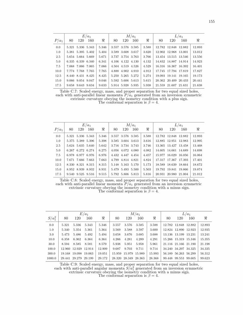
155

E/a1 M/a1 L/a1

P/a1 80 120 160 < 80 120 160 < 80 120 160 <0.0 5.321 5.336 5.343 5.346 3.557 3.576 3.585 3.588 12.782 12.848 12.882 12.893

1.0 5.381 5.395 5.402 5.404 3.589 3.608 3.617 3.620 12.902 12.968 13.001 13.012

2.5 5.654 5.664 5.669 5.671 3.737 3.754 3.763 3.766 13.454 13.515 13.546 13.556

5.0 6.335 6.339 6.340 6.341 4.106 4.122 4.130 4.132 14.832 14.887 14.914 14.923

7.5 7.068 7.066 7.065 7.066 4.504 4.519 4.526 4.529 16.316 16.367 16.392 16.401

10.0 7.774 7.768 7.765 7.765 4.888 4.902 4.910 4.912 17.745 17.794 17.819 17.827

12.5 8.440 8.431 8.425 8.425 5.250 5.265 5.272 5.274 19.093 19.141 19.165 19.173

15.0 9.066 9.054 9.047 9.046 5.592 5.606 5.613 5.615 20.362 20.409 20.433 20.441

17.5 9.658 9.643 9.634 9.633 5.914 5.928 5.935 5.938 21.559 21.607 21.631 21.638

Table C.7: Scaled energy, mass, and proper separation for two equal sized holes,each with anti-parallel linear momenta P/a1 generated from an inversion symmetric

extrinsic curvature obeying the isometry condition with a plus sign.The conformal separation is β = 4.

E/a1 M/a1 L/a1

P/a1 80 120 160 < 80 120 160 < 80 120 160 <0.0 5.321 5.336 5.343 5.346 3.557 3.576 3.585 3.588 12.782 12.848 12.882 12.893

1.0 5.375 5.389 5.396 5.398 3.585 3.604 3.613 3.616 12.885 12.951 12.983 12.995

2.5 5.624 5.635 5.640 5.642 3.716 3.734 3.743 3.746 13.365 13.427 13.458 13.468

5.0 6.267 6.272 6.274 6.275 4.056 4.072 4.080 4.082 14.605 14.661 14.689 14.698

7.5 6.978 6.977 6.976 6.976 4.432 4.447 4.454 4.457 15.977 16.029 16.056 16.064

10.0 7.671 7.666 7.663 7.663 4.799 4.814 4.821 4.824 17.317 17.367 17.393 17.401

12.5 8.330 8.321 8.315 8.315 5.148 5.163 5.170 5.173 18.589 18.639 18.664 18.672

15.0 8.952 8.939 8.932 8.931 5.479 5.493 5.500 5.503 19.792 19.841 19.866 19.874

17.5 9.540 9.525 9.516 9.515 5.792 5.806 5.813 5.816 20.931 20.980 21.004 21.012

Table C.8: Scaled energy, mass, and proper separation for two equal sized holes,each with anti-parallel linear momenta P/a1 generated from an inversion symmetric

extrinsic curvature obeying the isometry condition with a minus sign.The conformal separation is β = 4.

E/a1 M/a1 L/a1

S/a21 80 120 160 < 80 120 160 < 80 120 160 <

0.0 5.321 5.336 5.343 5.346 3.557 3.576 3.585 3.588 12.782 12.848 12.882 12.893

1.0 5.340 5.354 5.361 5.364 3.569 3.588 3.597 3.600 12.824 12.890 12.923 12.935

3.0 5.473 5.486 5.492 5.494 3.658 3.676 3.685 3.688 13.136 13.199 13.231 13.241

10.0 6.358 6.362 6.364 6.364 4.266 4.281 4.289 4.291 15.266 15.319 15.346 15.355

30.0 8.594 8.585 8.581 8.579 5.938 5.951 5.958 5.961 21.116 21.166 21.190 21.198

100.0 12.960 12.929 12.914 12.909 9.687 9.703 9.711 9.714 34.240 34.297 34.325 34.335

300.0 19.168 19.098 19.063 19.051 15.959 15.979 15.989 15.993 56.189 56.263 56.299 56.312

1000.0 29.441 29.279 29.199 29.172 28.320 28.349 28.363 28.368 99.448 99.553 99.605 99.623

Table C.9: Scaled energy, mass, and proper separation for two equal sized holes,each with anti-parallel angular momenta S/a2

1 generated from an inversion symmetricextrinsic curvature obeying the isometry condition with a minus sign.

The conformal separation is β = 4.

156

E/a1 M/a1 L/a1

P/a1 80 120 160 < 80 120 160 < 80 120 160 <0.0 5.321 5.336 5.343 5.346 3.557 3.576 3.585 3.588 12.782 12.848 12.882 12.893

1.0 5.819 5.844 5.856 5.860 3.675 3.694 3.704 3.707 13.206 13.273 13.306 13.317

2.5 7.778 7.859 7.901 7.913 4.115 4.134 4.144 4.147 14.781 14.850 14.884 14.896

5.0 11.953 12.221 12.363 12.399 4.949 4.972 4.983 4.987 17.774 17.853 17.891 17.905

7.5 16.205 16.752 17.048 17.116 5.714 5.740 5.752 5.757 20.518 20.608 20.651 20.667

10.0 20.299 21.193 21.688 21.790 6.402 6.431 6.445 6.450 22.983 23.085 23.134 23.153

12.5 24.195 25.490 26.219 26.354 7.027 7.059 7.075 7.081 25.226 25.340 25.394 25.415

15.0 27.898 29.633 30.626 30.789 7.603 7.639 7.656 7.662 27.292 27.418 27.477 27.501

17.5 31.421 33.624 34.905 35.093 8.139 8.178 8.197 8.204 29.216 29.353 29.418 29.444

Table C.10: Scaled energy, mass, and proper separation for two equal sized holes,each with parallel linear momenta P/a1 generated from an inversion symmetric

extrinsic curvature obeying the isometry condition with a plus sign.tThe conformal separation is β = 4.

E/a1 M/a1 L/a1

P/a1 80 120 160 < 80 120 160 < 80 120 160 <0.0 5.321 5.336 5.343 5.346 3.557 3.576 3.585 3.588 12.782 12.848 12.882 12.893

1.0 5.810 5.835 5.848 5.852 3.670 3.689 3.698 3.701 13.185 13.252 13.285 13.296

2.5 7.752 7.833 7.875 7.887 4.094 4.113 4.123 4.127 14.698 14.767 14.802 14.814

5.0 11.916 12.184 12.327 12.363 4.909 4.931 4.942 4.946 17.610 17.689 17.728 17.742

7.5 16.168 16.714 17.011 17.078 5.660 5.686 5.698 5.703 20.294 20.386 20.430 20.446

10.0 20.262 21.156 21.651 21.753 6.336 6.366 6.380 6.385 22.712 22.816 22.866 22.885

12.5 24.160 25.455 26.184 26.318 6.952 6.985 7.000 7.007 24.914 25.030 25.085 25.107

15.0 27.865 29.599 30.592 30.755 7.520 7.556 7.573 7.580 26.944 27.072 27.133 27.157

17.5 31.389 33.591 34.872 35.059 8.048 8.088 8.106 8.114 28.835 28.975 29.041 29.068

Table C.11: Scaled energy, mass, and proper separation for two equal sized holes,each with parallel linear momenta P/a1 generated from an inversion symmetric

extrinsic curvature obeying the isometry condition with a minus sign.The conformal separation is β = 4.

E/a1 M/a1 L/a1

S/a21 80 120 160 < 80 120 160 < 80 120 160 <

0.0 5.321 5.336 5.343 5.346 3.557 3.576 3.585 3.588 12.782 12.848 12.882 12.893

1.0 5.346 5.360 5.367 5.369 3.571 3.590 3.599 3.602 12.832 12.898 12.931 12.942

3.0 5.521 5.532 5.538 5.540 3.675 3.693 3.702 3.705 13.199 13.262 13.293 13.304

10.0 6.660 6.661 6.661 6.661 4.362 4.377 4.385 4.387 15.612 15.666 15.692 15.701

30.0 9.644 9.619 9.607 9.602 6.195 6.210 6.217 6.219 22.066 22.117 22.142 22.150

100.0 16.262 16.145 16.092 16.067 10.300 10.316 10.324 10.327 36.545 36.603 36.632 36.642

300.0 27.665 27.198 27.002 26.886 17.200 17.222 17.233 17.237 60.919 60.995 61.032 61.046

1000.0 52.050 50.110 49.220 48.817 30.859 30.891 30.906 30.913 109.198 109.308 109.362 109.382

Table C.12: Scaled energy, mass, and proper separation for two equal sized holes,each with parallel angular momenta S/a2

1 generated from an inversion symmetricextrinsic curvature obeying the isometry condition with a minus sign.

The conformal separation is β = 4.

157

E/a1 M/a1 L/a1

P/a1 80 120 160 < 80 120 160 < 80 120 160 <0.0 4.979 4.990 4.995 4.997 3.104 3.118 3.125 3.127 14.257 14.317 14.347 14.357

1.0 5.073 5.083 5.088 5.089 3.149 3.162 3.169 3.171 14.474 14.532 14.561 14.571

2.5 5.474 5.481 5.484 5.485 3.341 3.353 3.359 3.361 15.399 15.452 15.479 15.488

5.0 6.378 6.378 6.377 6.378 3.772 3.783 3.789 3.791 17.476 17.524 17.547 17.555

7.5 7.283 7.278 7.275 7.274 4.205 4.216 4.221 4.223 19.556 19.600 19.623 19.630

10.0 8.127 8.117 8.111 8.110 4.609 4.620 4.625 4.627 21.491 21.535 21.557 21.564

12.5 8.908 8.894 8.886 8.885 4.984 4.994 5.000 5.001 23.283 23.327 23.348 23.356

15.0 9.636 9.618 9.608 9.606 5.333 5.344 5.349 5.351 24.952 24.995 25.017 25.024

17.5 10.319 10.297 10.285 10.283 5.660 5.671 5.676 5.678 26.516 26.560 26.582 26.589

Table C.13: Scaled energy, mass, and proper separation for two equal sized holes,each with anti-parallel linear momenta P/a1 generated from an inversion symmetric

extrinsic curvature obeying the isometry condition with a plus sign.The conformal separation is β = 5.

E/a1 M/a1 L/a1

P/a1 80 120 160 < 80 120 160 < 80 120 160 <0.0 4.979 4.990 4.995 4.997 3.104 3.118 3.125 3.127 14.257 14.317 14.347 14.357

1.0 5.063 5.073 5.078 5.080 3.143 3.157 3.163 3.165 14.440 14.499 14.528 14.538

2.5 5.434 5.440 5.444 5.445 3.314 3.327 3.333 3.335 15.243 15.298 15.325 15.334

5.0 6.299 6.299 6.299 6.299 3.715 3.726 3.731 3.733 17.118 17.167 17.191 17.199

7.5 7.185 7.180 7.177 7.176 4.126 4.137 4.142 4.144 19.041 19.087 19.110 19.118

10.0 8.020 8.010 8.004 8.003 4.514 4.524 4.529 4.531 20.851 20.896 20.919 20.927

12.5 8.796 8.782 8.774 8.772 4.875 4.885 4.891 4.893 22.537 22.582 22.604 22.612

15.0 9.521 9.503 9.493 9.491 5.213 5.223 5.228 5.230 24.111 24.157 24.179 24.187

17.5 10.202 10.180 10.168 10.166 5.530 5.541 5.546 5.548 25.591 25.637 25.659 25.667

Table C.14: Scaled energy, mass, and proper separation for two equal sized holes,each with anti-parallel linear momenta P/a1 generated from an inversion symmetric

extrinsic curvature obeying the isometry condition with a minus sign.The conformal separation is β = 5.

E/a1 M/a1 L/a1

S/a21 80 120 160 < 80 120 160 < 80 120 160 <

0.0 4.979 4.990 4.995 4.997 3.104 3.118 3.125 3.127 14.257 14.317 14.347 14.357

1.0 5.005 5.016 5.021 5.023 3.120 3.133 3.140 3.142 14.325 14.384 14.414 14.424

3.0 5.193 5.201 5.206 5.207 3.230 3.243 3.249 3.251 14.807 14.863 14.891 14.901

10.0 6.292 6.293 6.294 6.294 3.902 3.913 3.918 3.920 17.739 17.787 17.810 17.819

30.0 8.800 8.790 8.785 8.783 5.581 5.591 5.596 5.598 25.065 25.112 25.135 25.143

100.0 13.535 13.504 13.488 13.482 9.235 9.247 9.253 9.255 41.020 41.077 41.104 41.114

300.0 20.218 20.147 20.112 20.100 15.307 15.323 15.331 15.333 67.535 67.610 67.647 67.660

1000.0 31.254 31.093 31.014 30.987 27.256 27.279 27.290 27.294 119.716 119.823 119.877 119.895

Table C.15: Scaled energy, mass, and proper separation for two equal sized holes,each with anti-parallel angular momenta S/a2

1 generated from an inversion symmetricextrinsic curvature obeying the isometry condition with a minus sign.

The conformal separation is β = 5.

158

E/a1 M/a1 L/a1

P/a1 80 120 160 < 80 120 160 < 80 120 160 <0.0 4.979 4.990 4.995 4.997 3.104 3.118 3.125 3.127 14.257 14.317 14.347 14.357

1.0 5.521 5.539 5.548 5.551 3.222 3.235 3.242 3.244 14.795 14.855 14.885 14.895

2.5 7.619 7.676 7.705 7.714 3.643 3.657 3.664 3.667 16.728 16.789 16.820 16.831

5.0 12.060 12.249 12.349 12.375 4.420 4.436 4.443 4.446 20.288 20.358 20.393 20.405

7.5 16.637 17.029 17.238 17.290 5.121 5.140 5.148 5.152 23.506 23.587 23.626 23.641

10.0 21.118 21.769 22.122 22.203 5.749 5.769 5.779 5.783 26.384 26.475 26.519 26.536

12.5 25.455 26.413 26.939 27.052 6.318 6.341 6.352 6.356 28.995 29.097 29.145 29.164

15.0 29.643 30.946 31.670 31.815 6.842 6.867 6.879 6.884 31.398 31.509 31.563 31.584

17.5 33.684 35.365 36.310 36.486 7.329 7.356 7.369 7.375 33.632 33.754 33.812 33.835

Table C.16: Scaled energy, mass, and proper separation for two equal sized holes,each with parallel linear momenta P/a1 generated from an inversion symmetric

extrinsic curvature obeying the isometry condition with a plus sign.The conformal separation is β = 5.

E/a1 M/a1 L/a1

P/a1 80 120 160 < 80 120 160 < 80 120 160 <0.0 4.979 4.990 4.995 4.997 3.104 3.118 3.125 3.127 14.257 14.317 14.347 14.357

1.0 5.510 5.528 5.537 5.540 3.215 3.229 3.235 3.238 14.760 14.820 14.850 14.860

2.5 7.586 7.643 7.673 7.681 3.619 3.633 3.640 3.642 16.595 16.657 16.688 16.699

5.0 12.016 12.205 12.305 12.332 4.373 4.390 4.398 4.400 20.028 20.100 20.136 20.148

7.5 16.593 16.985 17.194 17.246 5.060 5.078 5.087 5.091 23.154 23.237 23.277 23.292

10.0 21.075 21.726 22.079 22.161 5.675 5.696 5.706 5.710 25.957 26.051 26.096 26.113

12.5 25.414 26.372 26.898 27.011 6.234 6.257 6.268 6.273 28.504 28.608 28.658 28.678

15.0 29.604 30.907 31.631 31.776 6.748 6.774 6.786 6.791 30.849 30.964 31.019 31.041

17.5 33.647 35.328 36.273 36.449 7.227 7.255 7.268 7.274 33.032 33.158 33.217 33.241

Table C.17: Scaled energy, mass, and proper separation for two equal sized holes,each with parallel linear momenta P/a1 generated from an inversion symmetric

extrinsic curvature obeying the isometry condition with a minus sign.The conformal separation is β = 5.

E/a1 M/a1 L/a1

S/a21 80 120 160 < 80 120 160 < 80 120 160 <

0.0 4.979 4.990 4.995 4.997 3.104 3.118 3.125 3.127 14.257 14.317 14.347 14.357

1.0 5.010 5.021 5.026 5.028 3.121 3.135 3.141 3.144 14.331 14.391 14.420 14.431

3.0 5.230 5.239 5.243 5.244 3.241 3.254 3.260 3.262 14.857 14.913 14.940 14.950

10.0 6.525 6.524 6.523 6.523 3.958 3.968 3.973 3.975 17.995 18.043 18.066 18.074

30.0 9.638 9.616 9.605 9.601 5.730 5.741 5.746 5.748 25.784 25.831 25.854 25.863

100.0 16.303 16.209 16.165 16.146 9.606 9.619 9.625 9.627 42.870 42.927 42.955 42.965

300.0 27.577 27.211 27.056 26.966 16.086 16.103 16.111 16.114 71.502 71.577 71.614 71.627

1000.0 51.469 49.716 49.002 48.548 28.894 28.918 28.930 28.934 128.168 128.275 128.327 128.347

Table C.18: Scaled energy, mass, and proper separation for two equal sized holes,each with parallel angular momenta S/a2

1 generated from an inversion symmetricextrinsic curvature obeying the isometry condition with a minus sign.

The conformal separation is β = 5.

159

E/a1 M/a1 L/a1

P/a1 80 120 160 < 80 120 160 < 80 120 160 <0.0 4.778 4.787 4.792 4.794 2.856 2.867 2.873 2.875 15.670 15.728 15.756 15.766

1.0 4.906 4.914 4.918 4.919 2.912 2.922 2.928 2.930 15.989 16.045 16.073 16.082

2.5 5.424 5.428 5.430 5.431 3.136 3.146 3.151 3.153 17.283 17.333 17.358 17.367

5.0 6.510 6.507 6.506 6.505 3.607 3.616 3.621 3.622 19.987 20.032 20.054 20.062

7.5 7.554 7.546 7.541 7.540 4.061 4.070 4.074 4.075 22.583 22.626 22.647 22.655

10.0 8.510 8.497 8.489 8.488 4.476 4.485 4.490 4.491 24.957 25.000 25.021 25.029

12.5 9.388 9.370 9.360 9.358 4.858 4.867 4.872 4.873 27.137 27.179 27.201 27.208

15.0 10.202 10.179 10.167 10.164 5.213 5.222 5.226 5.228 29.155 29.198 29.220 29.227

17.5 10.962 10.936 10.921 10.918 5.544 5.553 5.557 5.559 31.041 31.084 31.106 31.113

Table C.19: Scaled energy, mass, and proper separation for two equal sized holes,each with anti-parallel linear momenta P/a1 generated from an inversion symmetric

extrinsic curvature obeying the isometry condition with a plus sign.The conformal separation is β = 6.

E/a1 M/a1 L/a1

P/a1 80 120 160 < 80 120 160 < 80 120 160 <0.0 4.778 4.787 4.792 4.794 2.856 2.867 2.873 2.875 15.670 15.728 15.756 15.766

1.0 4.893 4.902 4.906 4.907 2.904 2.915 2.920 2.922 15.940 15.996 16.024 16.034

2.5 5.375 5.380 5.382 5.382 3.106 3.116 3.121 3.123 17.068 17.120 17.145 17.154

5.0 6.423 6.421 6.419 6.419 3.545 3.555 3.559 3.561 19.522 19.569 19.592 19.600

7.5 7.452 7.443 7.439 7.438 3.978 3.987 3.991 3.993 21.931 21.976 21.998 22.006

10.0 8.400 8.387 8.379 8.378 4.377 4.386 4.390 4.392 24.156 24.201 24.223 24.230

12.5 9.275 9.256 9.247 9.244 4.746 4.755 4.759 4.761 26.207 26.252 26.274 26.282

15.0 10.087 10.064 10.051 10.049 5.089 5.098 5.102 5.104 28.113 28.158 28.180 28.188

17.5 10.846 10.819 10.804 10.801 5.410 5.419 5.423 5.425 29.896 29.942 29.964 29.972

Table C.20: Scaled energy, mass, and proper separation for two equal sized holes,each with anti-parallel linear momenta P/a1 generated from an inversion symmetric

extrinsic curvature obeying the isometry condition with a minus sign.The conformal separation is β = 6.

E/a1 M/a1 L/a1

S/a21 80 120 160 < 80 120 160 < 80 120 160 <

0.0 4.778 4.787 4.792 4.794 2.856 2.867 2.873 2.875 15.670 15.728 15.756 15.766

1.0 4.811 4.821 4.825 4.827 2.874 2.885 2.891 2.893 15.761 15.819 15.847 15.857

3.0 5.043 5.050 5.053 5.055 3.000 3.010 3.015 3.017 16.396 16.450 16.476 16.486

10.0 6.297 6.297 6.296 6.296 3.707 3.716 3.720 3.722 19.980 20.026 20.049 20.057

30.0 9.005 8.993 8.987 8.985 5.385 5.394 5.398 5.399 28.484 28.531 28.554 28.563

100.0 14.039 14.006 13.989 13.984 8.985 8.995 9.000 9.002 46.743 46.802 46.831 46.841

300.0 21.126 21.053 21.017 21.005 14.948 14.962 14.968 14.971 76.998 77.077 77.116 77.129

1000.0 32.827 32.664 32.582 32.555 26.673 26.692 26.702 26.705 136.499 136.615 136.672 136.692

Table C.21: Scaled energy, mass, and proper separation for two equal sized holes,each with anti-parallel angular momenta S/a2

1 generated from an inversion symmetricextrinsic curvature obeying the isometry condition with a minus sign.

The conformal separation is β = 6.

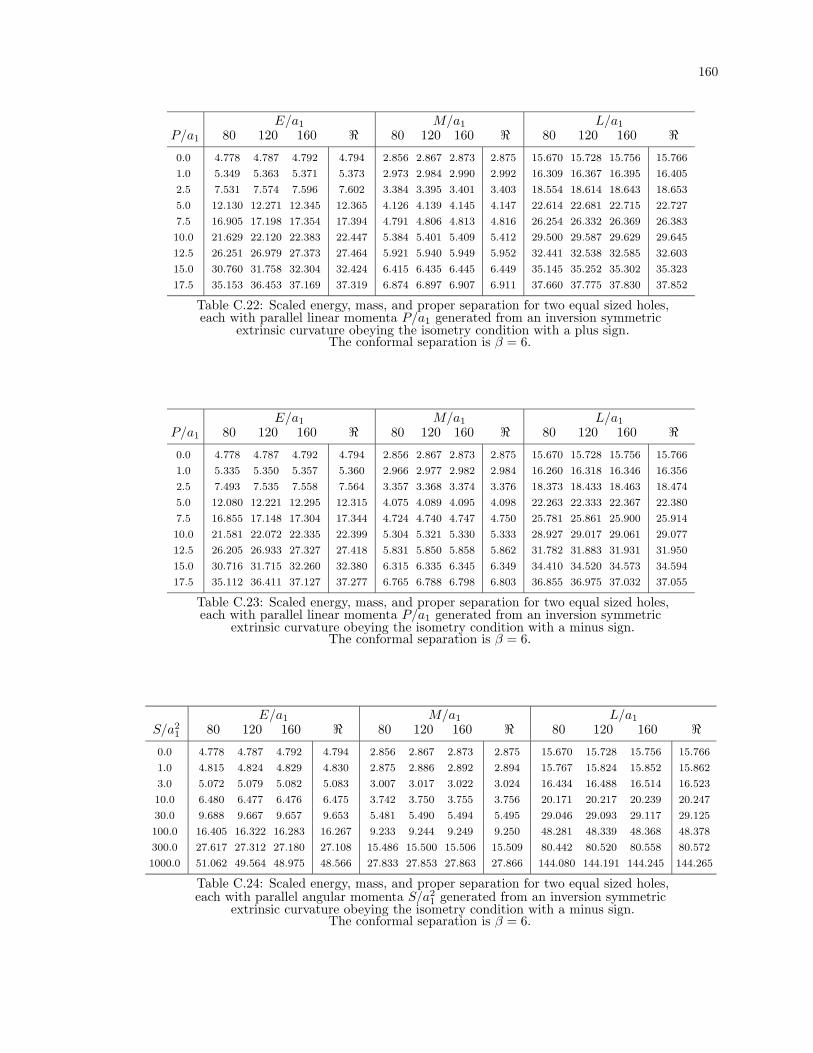
160

E/a1 M/a1 L/a1

P/a1 80 120 160 < 80 120 160 < 80 120 160 <0.0 4.778 4.787 4.792 4.794 2.856 2.867 2.873 2.875 15.670 15.728 15.756 15.766

1.0 5.349 5.363 5.371 5.373 2.973 2.984 2.990 2.992 16.309 16.367 16.395 16.405

2.5 7.531 7.574 7.596 7.602 3.384 3.395 3.401 3.403 18.554 18.614 18.643 18.653

5.0 12.130 12.271 12.345 12.365 4.126 4.139 4.145 4.147 22.614 22.681 22.715 22.727

7.5 16.905 17.198 17.354 17.394 4.791 4.806 4.813 4.816 26.254 26.332 26.369 26.383

10.0 21.629 22.120 22.383 22.447 5.384 5.401 5.409 5.412 29.500 29.587 29.629 29.645

12.5 26.251 26.979 27.373 27.464 5.921 5.940 5.949 5.952 32.441 32.538 32.585 32.603

15.0 30.760 31.758 32.304 32.424 6.415 6.435 6.445 6.449 35.145 35.252 35.302 35.323

17.5 35.153 36.453 37.169 37.319 6.874 6.897 6.907 6.911 37.660 37.775 37.830 37.852

Table C.22: Scaled energy, mass, and proper separation for two equal sized holes,each with parallel linear momenta P/a1 generated from an inversion symmetric

extrinsic curvature obeying the isometry condition with a plus sign.The conformal separation is β = 6.

E/a1 M/a1 L/a1

P/a1 80 120 160 < 80 120 160 < 80 120 160 <0.0 4.778 4.787 4.792 4.794 2.856 2.867 2.873 2.875 15.670 15.728 15.756 15.766

1.0 5.335 5.350 5.357 5.360 2.966 2.977 2.982 2.984 16.260 16.318 16.346 16.356

2.5 7.493 7.535 7.558 7.564 3.357 3.368 3.374 3.376 18.373 18.433 18.463 18.474

5.0 12.080 12.221 12.295 12.315 4.075 4.089 4.095 4.098 22.263 22.333 22.367 22.380

7.5 16.855 17.148 17.304 17.344 4.724 4.740 4.747 4.750 25.781 25.861 25.900 25.914

10.0 21.581 22.072 22.335 22.399 5.304 5.321 5.330 5.333 28.927 29.017 29.061 29.077

12.5 26.205 26.933 27.327 27.418 5.831 5.850 5.858 5.862 31.782 31.883 31.931 31.950

15.0 30.716 31.715 32.260 32.380 6.315 6.335 6.345 6.349 34.410 34.520 34.573 34.594

17.5 35.112 36.411 37.127 37.277 6.765 6.788 6.798 6.803 36.855 36.975 37.032 37.055

Table C.23: Scaled energy, mass, and proper separation for two equal sized holes,each with parallel linear momenta P/a1 generated from an inversion symmetric

extrinsic curvature obeying the isometry condition with a minus sign.The conformal separation is β = 6.

E/a1 M/a1 L/a1

S/a21 80 120 160 < 80 120 160 < 80 120 160 <

0.0 4.778 4.787 4.792 4.794 2.856 2.867 2.873 2.875 15.670 15.728 15.756 15.766

1.0 4.815 4.824 4.829 4.830 2.875 2.886 2.892 2.894 15.767 15.824 15.852 15.862

3.0 5.072 5.079 5.082 5.083 3.007 3.017 3.022 3.024 16.434 16.488 16.514 16.523

10.0 6.480 6.477 6.476 6.475 3.742 3.750 3.755 3.756 20.171 20.217 20.239 20.247

30.0 9.688 9.667 9.657 9.653 5.481 5.490 5.494 5.495 29.046 29.093 29.117 29.125

100.0 16.405 16.322 16.283 16.267 9.233 9.244 9.249 9.250 48.281 48.339 48.368 48.378

300.0 27.617 27.312 27.180 27.108 15.486 15.500 15.506 15.509 80.442 80.520 80.558 80.572

1000.0 51.062 49.564 48.975 48.566 27.833 27.853 27.863 27.866 144.080 144.191 144.245 144.265

Table C.24: Scaled energy, mass, and proper separation for two equal sized holes,each with parallel angular momenta S/a2

1 generated from an inversion symmetricextrinsic curvature obeying the isometry condition with a minus sign.

The conformal separation is β = 6.

161

E/a1 M/a1 L/a1

P/a1 80 120 160 < 80 120 160 < 80 120 160 <0.0 4.645 4.654 4.658 4.659 2.699 2.709 2.713 2.715 17.038 17.095 17.123 17.133

1.0 4.805 4.812 4.816 4.817 2.763 2.772 2.777 2.778 17.460 17.515 17.542 17.552

2.5 5.427 5.430 5.431 5.431 3.012 3.021 3.025 3.026 19.100 19.149 19.173 19.182

5.0 6.667 6.663 6.660 6.660 3.510 3.517 3.521 3.523 22.364 22.408 22.430 22.438

7.5 7.830 7.820 7.814 7.812 3.976 3.984 3.988 3.990 25.418 25.462 25.483 25.490

10.0 8.884 8.868 8.859 8.857 4.400 4.408 4.412 4.413 28.185 28.228 28.249 28.257

12.5 9.847 9.826 9.814 9.812 4.787 4.795 4.799 4.801 30.710 30.754 30.775 30.783

15.0 10.737 10.710 10.696 10.693 5.145 5.153 5.157 5.159 33.043 33.087 33.109 33.117

17.5 11.567 11.536 11.519 11.515 5.479 5.488 5.492 5.493 35.218 35.263 35.285 35.293

Table C.25: Scaled energy, mass, and proper separation for two equal sized holes,each with anti-parallel linear momenta P/a1 generated from an inversion symmetric

extrinsic curvature obeying the isometry condition with a plus sign.The conformal separation is β = 7.

E/a1 M/a1 L/a1

P/a1 80 120 160 < 80 120 160 < 80 120 160 <0.0 4.645 4.654 4.658 4.659 2.699 2.709 2.713 2.715 17.038 17.095 17.123 17.133

1.0 4.790 4.797 4.801 4.802 2.755 2.764 2.769 2.770 17.397 17.452 17.479 17.489

2.5 5.372 5.375 5.376 5.377 2.980 2.988 2.992 2.994 18.836 18.886 18.911 18.920

5.0 6.576 6.572 6.569 6.569 3.446 3.454 3.458 3.459 21.816 21.862 21.885 21.893

7.5 7.725 7.714 7.709 7.707 3.892 3.900 3.903 3.905 24.663 24.708 24.730 24.738

10.0 8.773 8.757 8.748 8.746 4.299 4.307 4.311 4.313 27.262 27.307 27.329 27.337

12.5 9.733 9.712 9.700 9.697 4.673 4.681 4.685 4.687 29.644 29.690 29.712 29.720

15.0 10.622 10.595 10.581 10.578 5.020 5.028 5.032 5.033 31.850 31.896 31.919 31.927

17.5 11.451 11.420 11.403 11.399 5.343 5.352 5.356 5.357 33.910 33.957 33.980 33.988

Table C.26: Scaled energy, mass, and proper separation for two equal sized holes,each with anti-parallel linear momenta P/a1 generated from an inversion symmetric

extrinsic curvature obeying the isometry condition with a minus sign.The conformal separation is β = 7.

E/a1 M/a1 L/a1

S/a21 80 120 160 < 80 120 160 < 80 120 160 <

0.0 4.645 4.654 4.658 4.659 2.699 2.709 2.713 2.715 17.038 17.095 17.123 17.133

1.0 4.685 4.693 4.697 4.698 2.719 2.729 2.733 2.735 17.152 17.208 17.235 17.246

3.0 4.952 4.958 4.961 4.962 2.855 2.864 2.868 2.870 17.921 17.974 17.999 18.009

10.0 6.324 6.322 6.321 6.321 3.585 3.592 3.596 3.597 22.046 22.092 22.114 22.122

30.0 9.189 9.176 9.170 9.168 5.261 5.268 5.272 5.273 31.531 31.580 31.604 31.612

100.0 14.476 14.442 14.425 14.420 8.826 8.835 8.839 8.841 51.733 51.795 51.825 51.836

300.0 21.917 21.843 21.806 21.793 14.719 14.731 14.737 14.739 85.156 85.241 85.283 85.297

1000.0 34.208 34.041 33.958 33.929 26.303 26.320 26.329 26.332 150.873 150.997 151.059 151.080

Table C.27: Scaled energy, mass, and proper separation for two equal sized holes,each with anti-parallel angular momenta S/a2

1 generated from an inversion symmetricextrinsic curvature obeying the isometry condition with a minus sign.

The conformal separation is β = 7.

162

E/a1 M/a1 L/a1

P/a1 80 120 160 < 80 120 160 < 80 120 160 <0.0 4.645 4.654 4.658 4.659 2.699 2.709 2.713 2.715 17.038 17.095 17.123 17.133

1.0 5.237 5.249 5.255 5.257 2.816 2.825 2.830 2.832 17.768 17.825 17.853 17.863

2.5 7.475 7.508 7.525 7.531 3.219 3.229 3.233 3.235 20.295 20.353 20.382 20.393

5.0 12.178 12.286 12.343 12.359 3.938 3.949 3.954 3.957 24.806 24.873 24.906 24.918

7.5 17.085 17.311 17.431 17.462 4.579 4.592 4.598 4.600 28.831 28.908 28.945 28.959

10.0 21.974 22.353 22.556 22.606 5.149 5.164 5.171 5.174 32.414 32.500 32.542 32.558

12.5 26.792 27.356 27.660 27.732 5.666 5.682 5.689 5.693 35.659 35.754 35.800 35.817

15.0 31.526 32.303 32.725 32.821 6.140 6.158 6.166 6.170 38.640 38.744 38.794 38.814

17.5 36.171 37.187 37.741 37.864 6.582 6.601 6.610 6.613 41.412 41.525 41.579 41.601

Table C.28: Scaled energy, mass, and proper separation for two equal sized holes,each with parallel linear momenta P/a1 generated from an inversion symmetric

extrinsic curvature obeying the isometry condition with a plus sign.The conformal separation is β = 7.

E/a1 M/a1 L/a1

P/a1 80 120 160 < 80 120 160 < 80 120 160 <0.0 4.645 4.654 4.658 4.659 2.699 2.709 2.713 2.715 17.038 17.095 17.123 17.133

1.0 5.221 5.233 5.239 5.241 2.807 2.817 2.821 2.823 17.706 17.763 17.791 17.801

2.5 7.432 7.465 7.483 7.488 3.190 3.200 3.204 3.206 20.069 20.129 20.159 20.169

5.0 12.122 12.231 12.289 12.304 3.884 3.896 3.901 3.904 24.375 24.445 24.478 24.491

7.5 17.030 17.256 17.376 17.407 4.509 4.522 4.528 4.531 28.252 28.331 28.369 28.384

10.0 21.921 22.300 22.503 22.553 5.066 5.080 5.088 5.090 31.713 31.803 31.846 31.862

12.5 26.742 27.306 27.610 27.682 5.571 5.587 5.595 5.598 34.854 34.953 35.000 35.019

15.0 31.478 32.255 32.677 32.773 6.035 6.053 6.061 6.065 37.743 37.851 37.903 37.924

17.5 36.125 37.141 37.696 37.818 6.467 6.486 6.495 6.499 40.430 40.548 40.604 40.627

Table C.29: Scaled energy, mass, and proper separation for two equal sized holes,each with parallel linear momenta P/a1 generated from an inversion symmetric

extrinsic curvature obeying the isometry condition with a minus sign.The conformal separation is β = 7.

E/a1 M/a1 L/a1

S/a21 80 120 160 < 80 120 160 < 80 120 160 <

0.0 4.645 4.654 4.658 4.659 2.699 2.709 2.713 2.715 17.038 17.095 17.123 17.133

1.0 4.688 4.696 4.700 4.701 2.720 2.729 2.734 2.736 17.156 17.212 17.239 17.249

3.0 4.975 4.981 4.983 4.984 2.860 2.869 2.873 2.875 17.950 18.002 18.028 18.037

10.0 6.469 6.466 6.464 6.464 3.608 3.615 3.619 3.620 22.191 22.237 22.260 22.268

30.0 9.756 9.736 9.726 9.723 5.326 5.333 5.337 5.338 31.982 32.031 32.055 32.063

100.0 16.527 16.452 16.416 16.402 9.001 9.011 9.015 9.017 53.044 53.105 53.136 53.147

300.0 27.712 27.448 27.331 27.271 15.113 15.125 15.131 15.133 88.217 88.300 88.340 88.355

1000.0 50.814 49.536 49.034 48.683 27.173 27.191 27.200 27.203 157.821 157.939 157.997 158.017

Table C.30: Scaled energy, mass, and proper separation for two equal sized holes,each with parallel angular momenta S/a2

1 generated from an inversion symmetricextrinsic curvature obeying the isometry condition with a minus sign.

The conformal separation is β = 7.

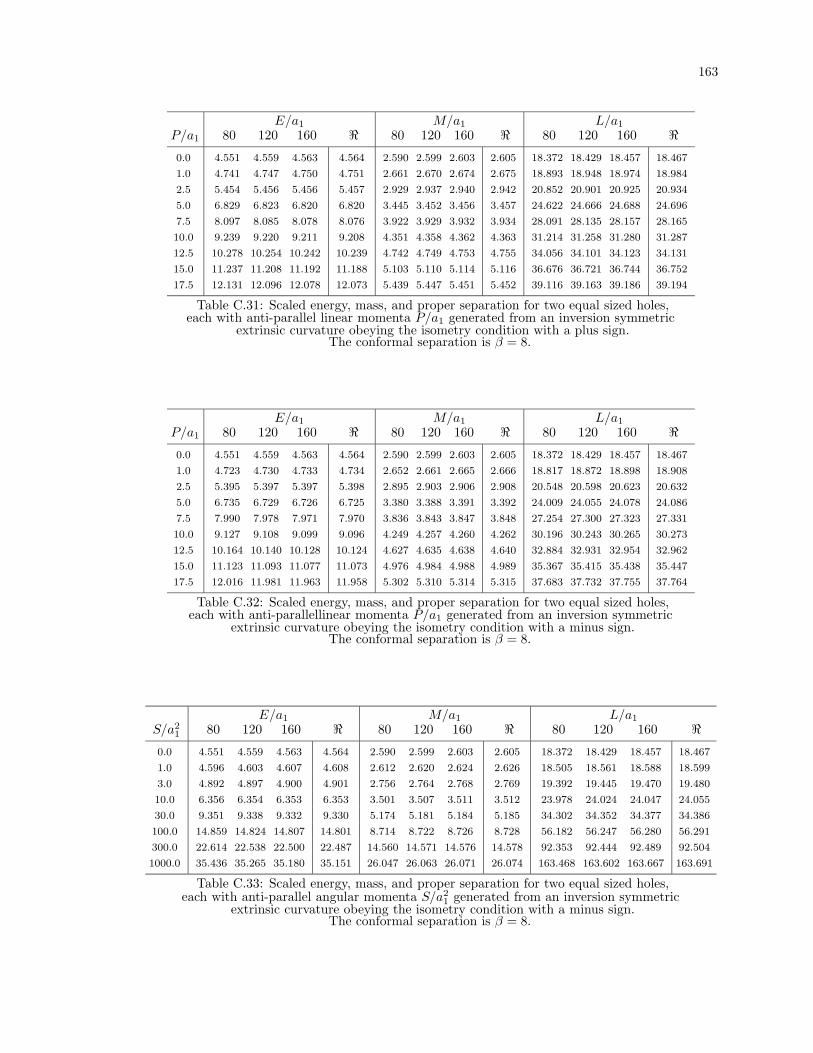
163

E/a1 M/a1 L/a1

P/a1 80 120 160 < 80 120 160 < 80 120 160 <0.0 4.551 4.559 4.563 4.564 2.590 2.599 2.603 2.605 18.372 18.429 18.457 18.467

1.0 4.741 4.747 4.750 4.751 2.661 2.670 2.674 2.675 18.893 18.948 18.974 18.984

2.5 5.454 5.456 5.456 5.457 2.929 2.937 2.940 2.942 20.852 20.901 20.925 20.934

5.0 6.829 6.823 6.820 6.820 3.445 3.452 3.456 3.457 24.622 24.666 24.688 24.696

7.5 8.097 8.085 8.078 8.076 3.922 3.929 3.932 3.934 28.091 28.135 28.157 28.165

10.0 9.239 9.220 9.211 9.208 4.351 4.358 4.362 4.363 31.214 31.258 31.280 31.287

12.5 10.278 10.254 10.242 10.239 4.742 4.749 4.753 4.755 34.056 34.101 34.123 34.131

15.0 11.237 11.208 11.192 11.188 5.103 5.110 5.114 5.116 36.676 36.721 36.744 36.752

17.5 12.131 12.096 12.078 12.073 5.439 5.447 5.451 5.452 39.116 39.163 39.186 39.194

Table C.31: Scaled energy, mass, and proper separation for two equal sized holes,each with anti-parallel linear momenta P/a1 generated from an inversion symmetric

extrinsic curvature obeying the isometry condition with a plus sign.The conformal separation is β = 8.

E/a1 M/a1 L/a1

P/a1 80 120 160 < 80 120 160 < 80 120 160 <0.0 4.551 4.559 4.563 4.564 2.590 2.599 2.603 2.605 18.372 18.429 18.457 18.467

1.0 4.723 4.730 4.733 4.734 2.652 2.661 2.665 2.666 18.817 18.872 18.898 18.908

2.5 5.395 5.397 5.397 5.398 2.895 2.903 2.906 2.908 20.548 20.598 20.623 20.632

5.0 6.735 6.729 6.726 6.725 3.380 3.388 3.391 3.392 24.009 24.055 24.078 24.086

7.5 7.990 7.978 7.971 7.970 3.836 3.843 3.847 3.848 27.254 27.300 27.323 27.331

10.0 9.127 9.108 9.099 9.096 4.249 4.257 4.260 4.262 30.196 30.243 30.265 30.273

12.5 10.164 10.140 10.128 10.124 4.627 4.635 4.638 4.640 32.884 32.931 32.954 32.962

15.0 11.123 11.093 11.077 11.073 4.976 4.984 4.988 4.989 35.367 35.415 35.438 35.447

17.5 12.016 11.981 11.963 11.958 5.302 5.310 5.314 5.315 37.683 37.732 37.755 37.764

Table C.32: Scaled energy, mass, and proper separation for two equal sized holes,each with anti-parallellinear momenta P/a1 generated from an inversion symmetric

extrinsic curvature obeying the isometry condition with a minus sign.The conformal separation is β = 8.

E/a1 M/a1 L/a1

S/a21 80 120 160 < 80 120 160 < 80 120 160 <

0.0 4.551 4.559 4.563 4.564 2.590 2.599 2.603 2.605 18.372 18.429 18.457 18.467

1.0 4.596 4.603 4.607 4.608 2.612 2.620 2.624 2.626 18.505 18.561 18.588 18.599

3.0 4.892 4.897 4.900 4.901 2.756 2.764 2.768 2.769 19.392 19.445 19.470 19.480

10.0 6.356 6.354 6.353 6.353 3.501 3.507 3.511 3.512 23.978 24.024 24.047 24.055

30.0 9.351 9.338 9.332 9.330 5.174 5.181 5.184 5.185 34.302 34.352 34.377 34.386

100.0 14.859 14.824 14.807 14.801 8.714 8.722 8.726 8.728 56.182 56.247 56.280 56.291

300.0 22.614 22.538 22.500 22.487 14.560 14.571 14.576 14.578 92.353 92.444 92.489 92.504

1000.0 35.436 35.265 35.180 35.151 26.047 26.063 26.071 26.074 163.468 163.602 163.667 163.691

Table C.33: Scaled energy, mass, and proper separation for two equal sized holes,each with anti-parallel angular momenta S/a2

1 generated from an inversion symmetricextrinsic curvature obeying the isometry condition with a minus sign.

The conformal separation is β = 8.

164

E/a1 M/a1 L/a1

P/a1 80 120 160 < 80 120 160 < 80 120 160 <0.0 4.551 4.559 4.563 4.564 2.590 2.599 2.603 2.605 18.372 18.429 18.457 18.467

1.0 5.157 5.168 5.173 5.175 2.707 2.715 2.719 2.721 19.185 19.242 19.269 19.279

2.5 7.436 7.463 7.477 7.481 3.104 3.113 3.117 3.119 21.967 22.026 22.055 22.065

5.0 12.212 12.298 12.343 12.355 3.807 3.817 3.822 3.824 26.894 26.961 26.993 27.005

7.5 17.212 17.391 17.485 17.510 4.431 4.442 4.448 4.450 31.275 31.352 31.389 31.403

10.0 22.219 22.517 22.677 22.716 4.985 4.998 5.005 5.007 35.171 35.257 35.299 35.314

12.5 27.179 27.623 27.862 27.919 5.487 5.502 5.508 5.511 38.698 38.792 38.838 38.856

15.0 32.076 32.689 33.021 33.097 5.948 5.964 5.971 5.974 41.938 42.041 42.091 42.111

17.5 36.906 37.709 38.145 38.243 6.376 6.393 6.401 6.405 44.949 45.062 45.115 45.137

Table C.34: Scaled energy, mass, and proper separation for two equal sized holes,each with parallel linear momenta P/a1 generated from an inversion symmetric

extrinsic curvature obeying the isometry condition with a plus sign.The conformal separation is β = 8.

E/a1 M/a1 L/a1

P/a1 80 120 160 < 80 120 160 < 80 120 160 <0.0 4.551 4.559 4.563 4.564 2.590 2.599 2.603 2.605 18.372 18.429 18.457 18.467

1.0 5.140 5.151 5.156 5.158 2.698 2.706 2.710 2.712 19.111 19.168 19.196 19.206

2.5 7.389 7.416 7.430 7.434 3.073 3.083 3.087 3.089 21.703 21.764 21.793 21.804

5.0 12.152 12.239 12.284 12.296 3.751 3.762 3.766 3.768 26.394 26.463 26.497 26.509

7.5 17.153 17.332 17.427 17.451 4.358 4.370 4.375 4.378 30.604 30.683 30.722 30.736

10.0 22.162 22.461 22.621 22.660 4.899 4.912 4.918 4.921 34.361 34.450 34.493 34.510

12.5 27.125 27.569 27.809 27.865 5.389 5.403 5.410 5.413 37.768 37.867 37.914 37.933

15.0 32.025 32.638 32.970 33.046 5.839 5.855 5.862 5.866 40.902 41.010 41.062 41.082

17.5 36.857 37.660 38.097 38.194 6.258 6.275 6.283 6.286 43.817 43.934 43.990 44.012

Table C.35: Scaled energy, mass, and proper separation for two equal sized holes,each with parallel linear momenta P/a1 generated from an inversion symmetric

extrinsic curvature obeying the isometry condition with a minus sign.The conformal separation is β = 8.

E/a1 M/a1 L/a1

S/a21 80 120 160 < 80 120 160 < 80 120 160 <

0.0 4.551 4.559 4.563 4.564 2.590 2.599 2.603 2.605 18.372 18.429 18.457 18.467

1.0 4.598 4.606 4.609 4.611 2.612 2.621 2.625 2.627 18.508 18.564 18.591 18.602

3.0 4.910 4.915 4.918 4.919 2.759 2.767 2.771 2.772 19.414 19.467 19.492 19.501

10.0 6.474 6.471 6.469 6.469 3.516 3.523 3.526 3.527 24.090 24.137 24.160 24.168

30.0 9.829 9.810 9.801 9.797 5.220 5.227 5.230 5.232 34.671 34.722 34.747 34.756

100.0 16.655 16.586 16.553 16.540 8.844 8.853 8.856 8.858 57.319 57.384 57.417 57.428

300.0 27.835 27.599 27.492 27.441 14.860 14.871 14.876 14.879 95.116 95.204 95.247 95.262

1000.0 50.682 49.576 49.137 48.839 26.727 26.743 26.751 26.754 169.926 170.052 170.114 170.136

Table C.36: Scaled energy, mass, and proper separation for two equal sized holes,each with parallel angular momenta S/a2

1 generated from an inversion symmetricextrinsic curvature obeying the isometry condition with a minus sign.

The conformal separation is β = 8.

165

E/a1 M/a1 L/a1

P/a1 80 120 160 < 80 120 160 < 80 120 160 <0.0 4.481 4.488 4.492 4.493 2.511 2.519 2.522 2.524 19.678 19.735 19.762 19.773

1.0 4.697 4.703 4.706 4.707 2.587 2.595 2.599 2.600 20.292 20.347 20.373 20.383

2.5 5.493 5.493 5.494 5.494 2.869 2.876 2.880 2.881 22.546 22.595 22.619 22.628

5.0 6.988 6.981 6.977 6.976 3.400 3.406 3.409 3.411 26.777 26.822 26.844 26.852

7.5 8.351 8.337 8.330 8.328 3.883 3.890 3.893 3.894 30.627 30.672 30.694 30.702

10.0 9.572 9.552 9.542 9.539 4.317 4.323 4.327 4.328 34.078 34.123 34.146 34.154

12.5 10.683 10.657 10.643 10.639 4.711 4.718 4.721 4.723 37.212 37.259 37.282 37.290

15.0 11.706 11.673 11.657 11.652 5.074 5.081 5.084 5.086 40.099 40.146 40.169 40.178

17.5 12.658 12.620 12.600 12.595 5.412 5.419 5.423 5.424 42.785 42.834 42.857 42.866

Table C.37: Scaled energy, mass, and proper separation for two equal sized holes,each with anti-parallel linear momenta P/a1 generated from an inversion symmetric

extrinsic curvature obeying the isometry condition with a plus sign.The conformal separation is β = 9.

E/a1 M/a1 L/a1

P/a1 80 120 160 < 80 120 160 < 80 120 160 <0.0 4.481 4.488 4.492 4.493 2.511 2.519 2.522 2.524 19.678 19.735 19.762 19.773

1.0 4.678 4.684 4.687 4.688 2.578 2.586 2.589 2.591 20.205 20.260 20.286 20.297

2.5 5.430 5.431 5.431 5.432 2.834 2.841 2.845 2.846 22.209 22.259 22.283 22.292

5.0 6.891 6.884 6.881 6.880 3.334 3.341 3.344 3.345 26.111 26.158 26.181 26.190

7.5 8.242 8.229 8.222 8.220 3.797 3.804 3.807 3.808 29.726 29.772 29.795 29.804

10.0 9.460 9.440 9.429 9.426 4.215 4.222 4.225 4.226 32.986 33.033 33.057 33.065

12.5 10.569 10.543 10.529 10.525 4.596 4.603 4.606 4.608 35.957 36.006 36.030 36.038

15.0 11.591 11.559 11.542 11.538 4.947 4.954 4.958 4.959 38.698 38.748 38.772 38.781

17.5 12.544 12.506 12.486 12.481 5.275 5.282 5.286 5.287 41.253 41.304 41.329 41.338

Table C.38: Scaled energy, mass, and proper separation for two equal sized holes,each with anti-parallel linear momenta P/a1 generated from an inversion symmetric

extrinsic curvature obeying the isometry condition with a minus sign.The conformal separation is β = 9.

E/a1 M/a1 L/a1

S/a21 80 120 160 < 80 120 160 < 80 120 160 <

0.0 4.481 4.488 4.492 4.493 2.511 2.519 2.522 2.524 19.678 19.735 19.762 19.773

1.0 4.530 4.537 4.540 4.541 2.533 2.541 2.545 2.546 19.828 19.884 19.912 19.922

3.0 4.850 4.855 4.857 4.858 2.684 2.691 2.694 2.696 20.820 20.872 20.898 20.907

10.0 6.390 6.387 6.386 6.386 3.439 3.445 3.448 3.449 25.803 25.850 25.874 25.882

30.0 9.494 9.481 9.475 9.473 5.110 5.116 5.119 5.120 36.859 36.911 36.937 36.946

100.0 15.196 15.161 15.143 15.137 8.632 8.639 8.643 8.644 60.214 60.284 60.318 60.330

300.0 23.234 23.157 23.119 23.106 14.443 14.453 14.458 14.460 98.810 98.907 98.955 98.971

1000.0 36.540 36.366 36.279 36.250 25.860 25.875 25.882 25.885 174.693 174.837 174.907 174.932

Table C.39: Scaled energy, mass, and proper separation for two equal sized holes,each with anti-parallel angular momenta S/a2

1 generated from an inversion symmetricextrinsic curvature obeying the isometry condition with a minus sign.

The conformal separation is β = 9.

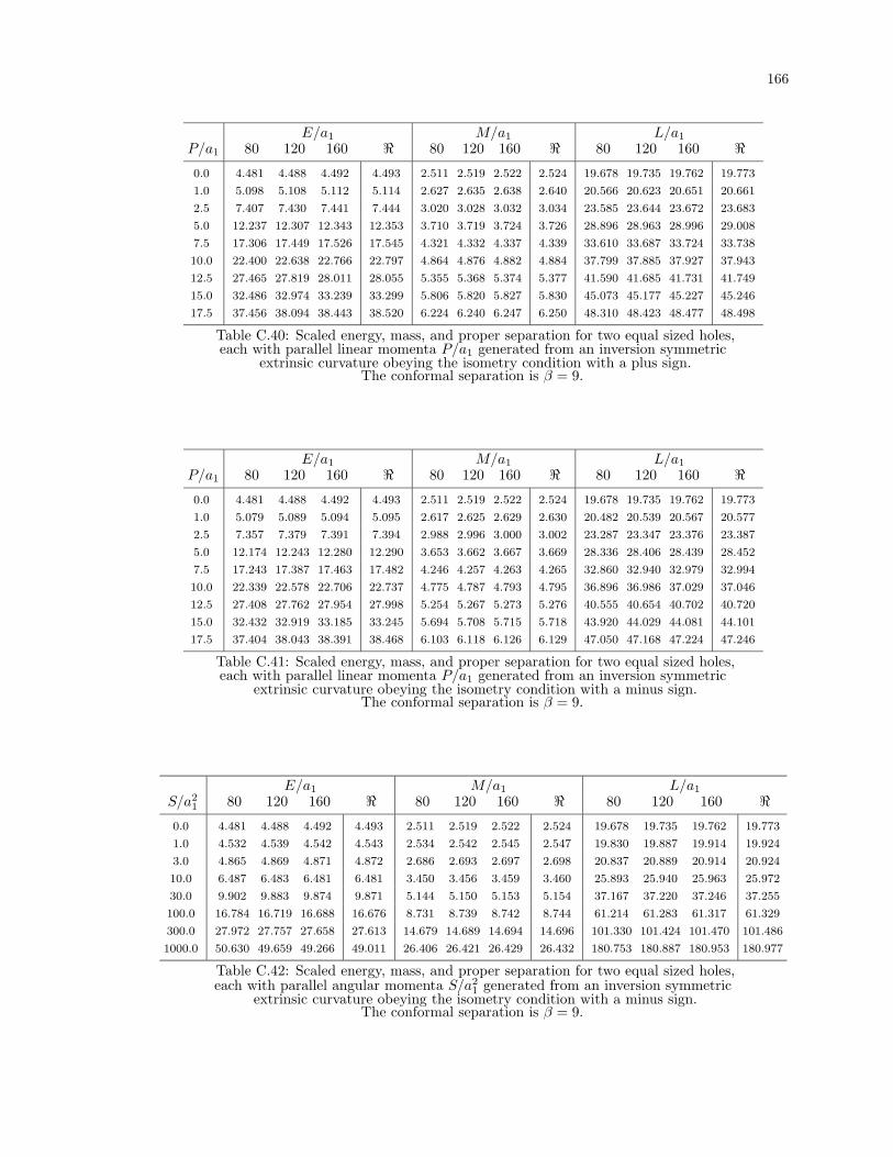
166

E/a1 M/a1 L/a1

P/a1 80 120 160 < 80 120 160 < 80 120 160 <0.0 4.481 4.488 4.492 4.493 2.511 2.519 2.522 2.524 19.678 19.735 19.762 19.773

1.0 5.098 5.108 5.112 5.114 2.627 2.635 2.638 2.640 20.566 20.623 20.651 20.661

2.5 7.407 7.430 7.441 7.444 3.020 3.028 3.032 3.034 23.585 23.644 23.672 23.683

5.0 12.237 12.307 12.343 12.353 3.710 3.719 3.724 3.726 28.896 28.963 28.996 29.008

7.5 17.306 17.449 17.526 17.545 4.321 4.332 4.337 4.339 33.610 33.687 33.724 33.738

10.0 22.400 22.638 22.766 22.797 4.864 4.876 4.882 4.884 37.799 37.885 37.927 37.943

12.5 27.465 27.819 28.011 28.055 5.355 5.368 5.374 5.377 41.590 41.685 41.731 41.749

15.0 32.486 32.974 33.239 33.299 5.806 5.820 5.827 5.830 45.073 45.177 45.227 45.246

17.5 37.456 38.094 38.443 38.520 6.224 6.240 6.247 6.250 48.310 48.423 48.477 48.498

Table C.40: Scaled energy, mass, and proper separation for two equal sized holes,each with parallel linear momenta P/a1 generated from an inversion symmetric

extrinsic curvature obeying the isometry condition with a plus sign.The conformal separation is β = 9.

E/a1 M/a1 L/a1

P/a1 80 120 160 < 80 120 160 < 80 120 160 <0.0 4.481 4.488 4.492 4.493 2.511 2.519 2.522 2.524 19.678 19.735 19.762 19.773

1.0 5.079 5.089 5.094 5.095 2.617 2.625 2.629 2.630 20.482 20.539 20.567 20.577

2.5 7.357 7.379 7.391 7.394 2.988 2.996 3.000 3.002 23.287 23.347 23.376 23.387

5.0 12.174 12.243 12.280 12.290 3.653 3.662 3.667 3.669 28.336 28.406 28.439 28.452

7.5 17.243 17.387 17.463 17.482 4.246 4.257 4.263 4.265 32.860 32.940 32.979 32.994

10.0 22.339 22.578 22.706 22.737 4.775 4.787 4.793 4.795 36.896 36.986 37.029 37.046

12.5 27.408 27.762 27.954 27.998 5.254 5.267 5.273 5.276 40.555 40.654 40.702 40.720

15.0 32.432 32.919 33.185 33.245 5.694 5.708 5.715 5.718 43.920 44.029 44.081 44.101

17.5 37.404 38.043 38.391 38.468 6.103 6.118 6.126 6.129 47.050 47.168 47.224 47.246

Table C.41: Scaled energy, mass, and proper separation for two equal sized holes,each with parallel linear momenta P/a1 generated from an inversion symmetric

extrinsic curvature obeying the isometry condition with a minus sign.The conformal separation is β = 9.

E/a1 M/a1 L/a1

S/a21 80 120 160 < 80 120 160 < 80 120 160 <

0.0 4.481 4.488 4.492 4.493 2.511 2.519 2.522 2.524 19.678 19.735 19.762 19.773

1.0 4.532 4.539 4.542 4.543 2.534 2.542 2.545 2.547 19.830 19.887 19.914 19.924

3.0 4.865 4.869 4.871 4.872 2.686 2.693 2.697 2.698 20.837 20.889 20.914 20.924

10.0 6.487 6.483 6.481 6.481 3.450 3.456 3.459 3.460 25.893 25.940 25.963 25.972

30.0 9.902 9.883 9.874 9.871 5.144 5.150 5.153 5.154 37.167 37.220 37.246 37.255

100.0 16.784 16.719 16.688 16.676 8.731 8.739 8.742 8.744 61.214 61.283 61.317 61.329

300.0 27.972 27.757 27.658 27.613 14.679 14.689 14.694 14.696 101.330 101.424 101.470 101.486

1000.0 50.630 49.659 49.266 49.011 26.406 26.421 26.429 26.432 180.753 180.887 180.953 180.977

Table C.42: Scaled energy, mass, and proper separation for two equal sized holes,each with parallel angular momenta S/a2

1 generated from an inversion symmetricextrinsic curvature obeying the isometry condition with a minus sign.

The conformal separation is β = 9.

167

E/a1 M/a1 L/a1

P/a1 80 120 160 < 80 120 160 < 80 120 160 <0.0 4.426 4.433 4.436 4.438 2.450 2.457 2.461 2.462 20.960 21.017 21.045 21.056

1.0 4.668 4.673 4.675 4.676 2.531 2.538 2.542 2.543 21.662 21.717 21.743 21.754

2.5 5.536 5.537 5.536 5.537 2.824 2.831 2.834 2.835 24.188 24.237 24.261 24.270

5.0 7.140 7.132 7.128 7.127 3.365 3.372 3.375 3.376 28.843 28.889 28.912 28.920

7.5 8.590 8.575 8.567 8.565 3.854 3.861 3.864 3.865 33.047 33.093 33.116 33.124

10.0 9.886 9.864 9.853 9.850 4.291 4.298 4.301 4.302 36.803 36.850 36.873 36.882

12.5 11.062 11.034 11.019 11.015 4.688 4.695 4.698 4.699 40.211 40.259 40.283 40.291

15.0 12.145 12.110 12.092 12.087 5.053 5.060 5.063 5.064 43.346 43.396 43.420 43.429

17.5 13.152 13.111 13.090 13.084 5.392 5.399 5.403 5.404 46.263 46.313 46.338 46.347

Table C.43: Scaled energy, mass, and proper separation for two equal sized holes,each with anti-parallel linear momenta P/a1 generated from an inversion symmetric

extrinsic curvature obeying the isometry condition with a plus sign.The conformal separation is β = 10.

E/a1 M/a1 L/a1

P/a1 80 120 160 < 80 120 160 < 80 120 160 <0.0 4.426 4.433 4.436 4.438 2.450 2.457 2.461 2.462 20.960 21.017 21.045 21.056

1.0 4.647 4.653 4.655 4.656 2.521 2.528 2.532 2.533 21.565 21.620 21.647 21.657

2.5 5.471 5.471 5.471 5.472 2.789 2.795 2.798 2.800 23.822 23.873 23.897 23.907

5.0 7.042 7.034 7.030 7.029 3.299 3.306 3.309 3.310 28.135 28.183 28.206 28.215

7.5 8.481 8.466 8.458 8.456 3.768 3.774 3.777 3.779 32.093 32.141 32.164 32.173

10.0 9.774 9.752 9.740 9.737 4.189 4.196 4.199 4.200 35.651 35.700 35.724 35.732

12.5 10.949 10.920 10.906 10.901 4.572 4.579 4.583 4.584 38.888 38.939 38.963 38.972

15.0 12.031 11.996 11.978 11.973 4.926 4.933 4.936 4.938 41.872 41.924 41.949 41.958

17.5 13.039 12.998 12.977 12.971 5.255 5.262 5.266 5.267 44.651 44.704 44.730 44.739

Table C.44: Scaled energy, mass, and proper separation for two equal sized holes,each with anti-parallel linear momenta P/a1 generated from an inversion symmetric

extrinsic curvature obeying the isometry condition with a minus sign.The conformal separation is β = 10.

E/a1 M/a1 L/a1

S/a21 80 120 160 < 80 120 160 < 80 120 160 <

0.0 4.426 4.433 4.436 4.438 2.450 2.457 2.461 2.462 20.960 21.017 21.045 21.056

1.0 4.479 4.485 4.488 4.490 2.473 2.481 2.484 2.486 21.126 21.182 21.210 21.220

3.0 4.819 4.824 4.826 4.826 2.629 2.635 2.639 2.640 22.210 22.263 22.288 22.298

10.0 6.422 6.419 6.417 6.417 3.392 3.397 3.400 3.401 27.544 27.592 27.616 27.624

30.0 9.621 9.608 9.601 9.599 5.061 5.066 5.069 5.070 39.247 39.302 39.328 39.338

100.0 15.496 15.460 15.442 15.436 8.568 8.575 8.579 8.580 63.917 63.990 64.026 64.039

300.0 23.791 23.713 23.674 23.661 14.353 14.363 14.368 14.369 104.680 104.783 104.833 104.851

1000.0 37.541 37.364 37.276 37.246 25.717 25.732 25.739 25.741 184.832 184.985 185.060 185.087

Table C.45: Scaled energy, mass, and proper separation for two equal sized holes,each with anti-parallel angular momenta S/a2

1 generated from an inversion symmetricextrinsic curvature obeying the isometry condition with a minus sign.

The conformal separation is β = 10.

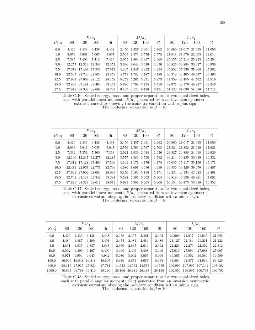
168

E/a1 M/a1 L/a1

P/a1 80 120 160 < 80 120 160 < 80 120 160 <0.0 4.426 4.433 4.436 4.438 2.450 2.457 2.461 2.462 20.960 21.017 21.045 21.056

1.0 5.053 5.061 5.065 5.067 2.565 2.573 2.576 2.578 21.918 21.976 22.003 22.014

2.5 7.385 7.404 7.413 7.416 2.955 2.963 2.967 2.968 25.155 25.214 25.243 25.254

5.0 12.257 12.313 12.343 12.351 3.636 3.644 3.649 3.650 30.826 30.894 30.927 30.939

7.5 17.378 17.494 17.556 17.571 4.237 4.247 4.252 4.254 35.852 35.930 35.968 35.982

10.0 22.537 22.730 22.834 22.859 4.771 4.782 4.787 4.789 40.318 40.405 40.447 40.463

12.5 27.684 27.969 28.123 28.158 5.253 5.265 5.271 5.273 44.359 44.455 44.502 44.519

15.0 32.800 33.191 33.404 33.451 5.696 5.709 5.715 5.718 48.071 48.176 48.227 48.246

17.5 37.878 38.389 38.669 38.729 6.107 6.122 6.128 6.131 51.522 51.636 51.690 51.711

Table C.46: Scaled energy, mass, and proper separation for two equal sized holes,each with parallel linear momenta P/a1 generated from an inversion symmetric

extrinsic curvature obeying the isometry condition with a plus sign.The conformal separation is β = 10.

E/a1 M/a1 L/a1

P/a1 80 120 160 < 80 120 160 < 80 120 160 <0.0 4.426 4.433 4.436 4.438 2.450 2.457 2.461 2.462 20.960 21.017 21.045 21.056

1.0 5.033 5.041 5.045 5.047 2.556 2.563 2.567 2.568 21.824 21.882 21.910 21.921

2.5 7.332 7.351 7.360 7.363 2.922 2.930 2.934 2.936 24.827 24.888 24.918 24.929

5.0 12.190 12.247 12.277 12.285 3.577 3.586 3.590 3.592 30.214 30.285 30.319 30.332

7.5 17.312 17.428 17.490 17.506 4.161 4.171 4.176 4.178 35.036 35.117 35.156 35.171

10.0 22.474 22.667 22.771 22.796 4.680 4.691 4.696 4.699 39.336 39.426 39.470 39.487

12.5 27.624 27.909 28.064 28.099 5.150 5.162 5.168 5.171 43.234 43.334 43.382 43.401

15.0 32.742 33.134 33.348 33.394 5.582 5.595 5.602 5.604 46.819 46.929 46.981 47.002

17.5 37.823 38.334 38.615 38.675 5.983 5.998 6.005 6.008 50.154 50.273 50.330 50.352

Table C.47: Scaled energy, mass, and proper separation for two equal sized holes,each with parallel linear momenta P/a1 generated from an inversion symmetric

extrinsic curvature obeying the isometry condition with a minus sign.The conformal separation is β = 10.

E/a1 M/a1 L/a1

S/a21 80 120 160 < 80 120 160 < 80 120 160 <

0.0 4.426 4.433 4.436 4.438 2.450 2.457 2.461 2.462 20.960 21.017 21.045 21.056

1.0 4.480 4.487 4.490 4.491 2.474 2.481 2.484 2.486 21.127 21.184 21.211 21.222

3.0 4.831 4.835 4.837 4.838 2.630 2.637 2.640 2.642 22.223 22.276 22.302 22.312

10.0 6.502 6.499 6.497 6.496 3.400 3.406 3.408 3.409 27.616 27.664 27.688 27.697

30.0 9.971 9.954 9.945 9.942 5.086 5.092 5.095 5.096 39.507 39.562 39.589 39.599

100.0 16.909 16.848 16.818 16.807 8.646 8.653 8.657 8.658 64.804 64.877 64.913 64.926

300.0 28.115 27.917 27.824 27.784 14.543 14.552 14.557 14.559 106.996 107.095 107.144 107.162

1000.0 50.634 49.768 49.410 49.190 26.166 26.181 26.187 26.190 190.554 190.697 190.767 190.792

Table C.48: Scaled energy, mass, and proper separation for two equal sized holes,each with parallel angular momenta S/a2

1 generated from an inversion symmetricextrinsic curvature obeying the isometry condition with a minus sign.

The conformal separation is β = 10.

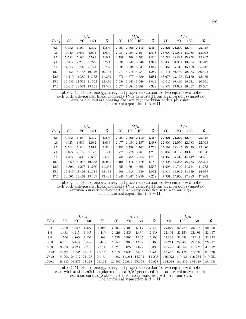
169

E/a1 M/a1 L/a1

P/a1 80 120 160 < 80 120 160 < 80 120 160 <0.0 4.382 4.389 4.392 4.394 2.401 2.409 2.412 2.413 22.221 22.279 22.307 22.318

1.0 4.646 4.651 4.654 4.655 2.487 2.494 2.497 2.498 23.006 23.061 23.088 23.098

2.5 5.582 5.582 5.581 5.581 2.789 2.796 2.798 2.800 25.784 25.834 25.858 25.867

5.0 7.285 7.276 7.272 7.271 3.339 3.345 3.348 3.349 30.833 30.881 30.904 30.912

7.5 8.815 8.799 8.791 8.789 3.832 3.838 3.841 3.842 35.367 35.415 35.438 35.447

10.0 10.181 10.158 10.146 10.142 4.271 4.278 4.281 4.282 39.411 39.459 39.483 39.492

12.5 11.419 11.389 11.373 11.369 4.670 4.677 4.680 4.681 43.075 43.125 43.150 43.159

15.0 12.558 12.521 12.502 12.496 5.036 5.043 5.046 5.048 46.445 46.496 46.521 46.531

17.5 13.617 13.574 13.551 13.545 5.377 5.384 5.388 5.389 49.579 49.632 49.657 49.667

Table C.49: Scaled energy, mass, and proper separation for two equal sized holes,each with anti-parallel linear momenta P/a1 generated from an inversion symmetric

extrinsic curvature obeying the isometry condition with a plus sign.The conformal separation is β = 11.

E/a1 M/a1 L/a1

P/a1 80 120 160 < 80 120 160 < 80 120 160 <0.0 4.382 4.389 4.392 4.394 2.401 2.409 2.412 2.413 22.221 22.279 22.307 22.318

1.0 4.625 4.630 4.632 4.633 2.477 2.484 2.487 2.488 22.900 22.956 22.983 22.993

2.5 5.514 5.514 5.514 5.514 2.753 2.759 2.762 2.764 25.394 25.445 25.470 25.480

5.0 7.186 7.177 7.173 7.171 3.272 3.278 3.281 3.283 30.089 30.138 30.161 30.170

7.5 8.706 8.690 8.682 8.680 3.745 3.752 3.755 3.756 34.369 34.418 34.442 34.451

10.0 10.069 10.045 10.033 10.030 4.169 4.176 4.179 4.180 38.208 38.258 38.283 38.292

12.5 11.306 11.276 11.260 11.256 4.555 4.561 4.565 4.566 41.696 41.749 41.774 41.783

15.0 12.445 12.408 12.389 12.383 4.909 4.916 4.920 4.921 44.910 44.963 44.989 44.999

17.5 13.505 13.461 13.439 13.432 5.240 5.247 5.250 5.252 47.901 47.956 47.983 47.993

Table C.50: Scaled energy, mass, and proper separation for two equal sized holes,each with anti-parallel linear momenta P/a1 generated from an inversion symmetric

extrinsic curvature obeying the isometry condition with a minus sign.The conformal separation is β = 11.

E/a1 M/a1 L/a1

S/a21 80 120 160 < 80 120 160 < 80 120 160 <

0.0 4.382 4.389 4.392 4.394 2.401 2.409 2.412 2.413 22.221 22.279 22.307 22.318

1.0 4.438 4.445 4.447 4.449 2.426 2.433 2.436 2.438 22.402 22.459 22.486 22.497

3.0 4.796 4.800 4.802 4.803 2.585 2.592 2.595 2.596 23.569 23.623 23.648 23.658

10.0 6.451 6.448 6.447 6.446 3.354 3.360 3.362 3.363 29.214 29.264 29.288 29.297

30.0 9.733 9.720 9.713 9.711 5.021 5.027 5.029 5.030 41.498 41.554 41.582 41.592

100.0 15.764 15.728 15.710 15.704 8.518 8.525 8.528 8.529 67.351 67.428 67.466 67.480

300.0 24.296 24.217 24.178 24.164 14.282 14.291 14.296 14.298 110.073 110.181 110.234 110.253

1000.0 38.455 38.277 38.188 38.157 25.605 25.619 25.625 25.628 194.088 194.250 194.329 194.358

Table C.51: Scaled energy, mass, and proper separation for two equal sized holes,each with anti-parallel angular momenta S/a2

1 generated from an inversion symmetricextrinsic curvature obeying the isometry condition with a minus sign.

The conformal separation is β = 11.

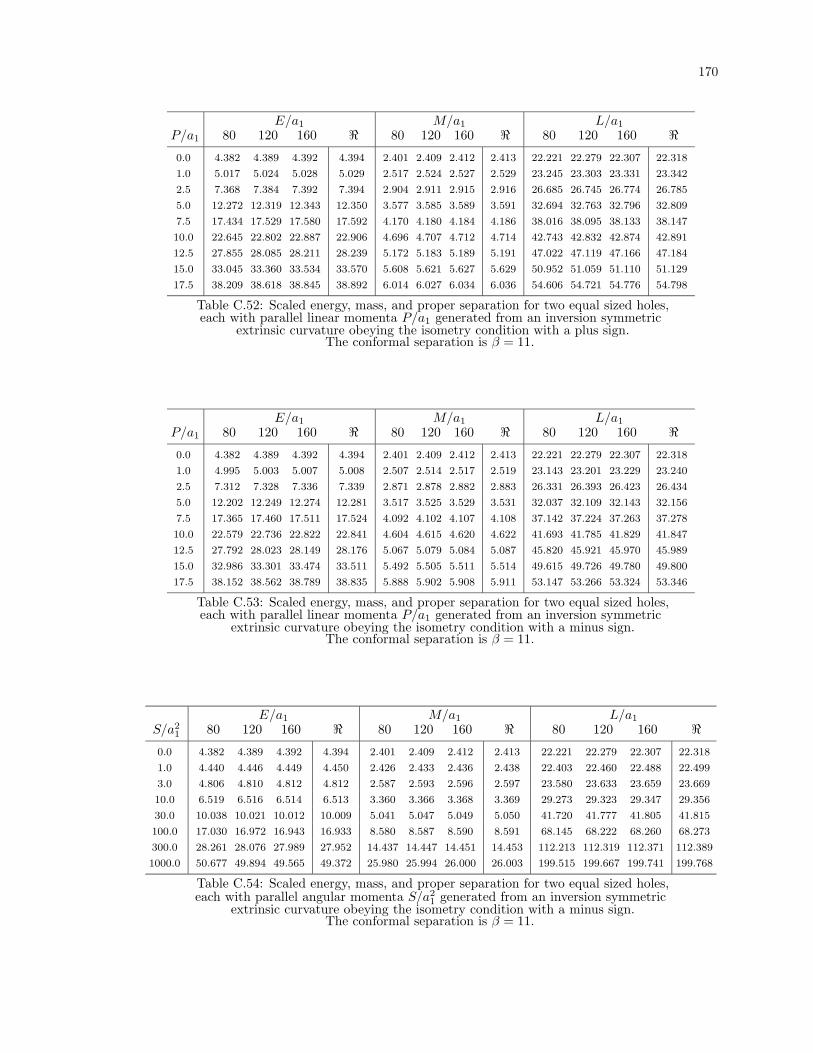
170

E/a1 M/a1 L/a1

P/a1 80 120 160 < 80 120 160 < 80 120 160 <0.0 4.382 4.389 4.392 4.394 2.401 2.409 2.412 2.413 22.221 22.279 22.307 22.318

1.0 5.017 5.024 5.028 5.029 2.517 2.524 2.527 2.529 23.245 23.303 23.331 23.342

2.5 7.368 7.384 7.392 7.394 2.904 2.911 2.915 2.916 26.685 26.745 26.774 26.785

5.0 12.272 12.319 12.343 12.350 3.577 3.585 3.589 3.591 32.694 32.763 32.796 32.809

7.5 17.434 17.529 17.580 17.592 4.170 4.180 4.184 4.186 38.016 38.095 38.133 38.147

10.0 22.645 22.802 22.887 22.906 4.696 4.707 4.712 4.714 42.743 42.832 42.874 42.891

12.5 27.855 28.085 28.211 28.239 5.172 5.183 5.189 5.191 47.022 47.119 47.166 47.184

15.0 33.045 33.360 33.534 33.570 5.608 5.621 5.627 5.629 50.952 51.059 51.110 51.129

17.5 38.209 38.618 38.845 38.892 6.014 6.027 6.034 6.036 54.606 54.721 54.776 54.798

Table C.52: Scaled energy, mass, and proper separation for two equal sized holes,each with parallel linear momenta P/a1 generated from an inversion symmetric

extrinsic curvature obeying the isometry condition with a plus sign.The conformal separation is β = 11.

E/a1 M/a1 L/a1

P/a1 80 120 160 < 80 120 160 < 80 120 160 <0.0 4.382 4.389 4.392 4.394 2.401 2.409 2.412 2.413 22.221 22.279 22.307 22.318

1.0 4.995 5.003 5.007 5.008 2.507 2.514 2.517 2.519 23.143 23.201 23.229 23.240

2.5 7.312 7.328 7.336 7.339 2.871 2.878 2.882 2.883 26.331 26.393 26.423 26.434

5.0 12.202 12.249 12.274 12.281 3.517 3.525 3.529 3.531 32.037 32.109 32.143 32.156

7.5 17.365 17.460 17.511 17.524 4.092 4.102 4.107 4.108 37.142 37.224 37.263 37.278

10.0 22.579 22.736 22.822 22.841 4.604 4.615 4.620 4.622 41.693 41.785 41.829 41.847

12.5 27.792 28.023 28.149 28.176 5.067 5.079 5.084 5.087 45.820 45.921 45.970 45.989

15.0 32.986 33.301 33.474 33.511 5.492 5.505 5.511 5.514 49.615 49.726 49.780 49.800

17.5 38.152 38.562 38.789 38.835 5.888 5.902 5.908 5.911 53.147 53.266 53.324 53.346

Table C.53: Scaled energy, mass, and proper separation for two equal sized holes,each with parallel linear momenta P/a1 generated from an inversion symmetric

extrinsic curvature obeying the isometry condition with a minus sign.The conformal separation is β = 11.

E/a1 M/a1 L/a1

S/a21 80 120 160 < 80 120 160 < 80 120 160 <

0.0 4.382 4.389 4.392 4.394 2.401 2.409 2.412 2.413 22.221 22.279 22.307 22.318

1.0 4.440 4.446 4.449 4.450 2.426 2.433 2.436 2.438 22.403 22.460 22.488 22.499

3.0 4.806 4.810 4.812 4.812 2.587 2.593 2.596 2.597 23.580 23.633 23.659 23.669

10.0 6.519 6.516 6.514 6.513 3.360 3.366 3.368 3.369 29.273 29.323 29.347 29.356

30.0 10.038 10.021 10.012 10.009 5.041 5.047 5.049 5.050 41.720 41.777 41.805 41.815

100.0 17.030 16.972 16.943 16.933 8.580 8.587 8.590 8.591 68.145 68.222 68.260 68.273

300.0 28.261 28.076 27.989 27.952 14.437 14.447 14.451 14.453 112.213 112.319 112.371 112.389

1000.0 50.677 49.894 49.565 49.372 25.980 25.994 26.000 26.003 199.515 199.667 199.741 199.768

Table C.54: Scaled energy, mass, and proper separation for two equal sized holes,each with parallel angular momenta S/a2

1 generated from an inversion symmetricextrinsic curvature obeying the isometry condition with a minus sign.

The conformal separation is β = 11.

171

E/a1 M/a1 L/a1

P/a1 80 120 160 < 80 120 160 < 80 120 160 <0.0 4.347 4.353 4.356 4.358 2.362 2.369 2.372 2.374 23.466 23.524 23.552 23.564

1.0 4.631 4.636 4.638 4.639 2.451 2.458 2.461 2.462 24.327 24.383 24.410 24.420

2.5 5.628 5.627 5.626 5.626 2.761 2.767 2.770 2.771 27.339 27.390 27.414 27.424

5.0 7.422 7.413 7.408 7.407 3.317 3.323 3.326 3.327 32.757 32.806 32.829 32.838

7.5 9.028 9.011 9.003 9.000 3.814 3.820 3.823 3.824 37.602 37.651 37.675 37.684

10.0 10.459 10.435 10.422 10.418 4.256 4.262 4.265 4.266 41.916 41.967 41.991 42.000

12.5 11.755 11.724 11.707 11.703 4.656 4.662 4.665 4.667 45.824 45.876 45.901 45.910

15.0 12.947 12.909 12.889 12.883 5.024 5.030 5.033 5.035 49.416 49.469 49.495 49.505

17.5 14.056 14.010 13.987 13.980 5.365 5.372 5.376 5.377 52.755 52.810 52.837 52.847

Table C.55: Scaled energy, mass, and proper separation for two equal sized holes,each with anti-parallel linear momenta P/a1 generated from an inversion symmetric

extrinsic curvature obeying the isometry condition with a plus sign.The conformal separation is β = 12.

E/a1 M/a1 L/a1

P/a1 80 120 160 < 80 120 160 < 80 120 160 <0.0 4.347 4.353 4.356 4.358 2.362 2.369 2.372 2.374 23.466 23.524 23.552 23.564

1.0 4.609 4.613 4.616 4.617 2.441 2.447 2.450 2.452 24.213 24.270 24.297 24.308

2.5 5.558 5.558 5.557 5.557 2.724 2.730 2.733 2.734 26.929 26.981 27.006 27.016

5.0 7.322 7.313 7.308 7.307 3.251 3.257 3.259 3.261 31.982 32.032 32.056 32.065

7.5 8.919 8.902 8.893 8.891 3.727 3.733 3.736 3.738 36.566 36.617 36.642 36.651

10.0 10.347 10.322 10.310 10.306 4.154 4.160 4.163 4.164 40.670 40.723 40.748 40.758

12.5 11.642 11.611 11.595 11.590 4.541 4.547 4.550 4.552 44.398 44.452 44.478 44.488

15.0 12.835 12.796 12.776 12.770 4.897 4.904 4.907 4.908 47.829 47.885 47.912 47.922

17.5 13.944 13.898 13.875 13.868 5.228 5.235 5.238 5.240 51.022 51.080 51.108 51.118

Table C.56: Scaled energy, mass, and proper separation for two equal sized holes,each with anti-parallel linear momenta P/a1 generated from an inversion symmetric

extrinsic curvature obeying the isometry condition with a minus sign.The conformal separation is β = 12.

E/a1 M/a1 L/a1

S/a21 80 120 160 < 80 120 160 < 80 120 160 <

0.0 4.347 4.353 4.356 4.358 2.362 2.369 2.372 2.374 23.466 23.524 23.552 23.564

1.0 4.405 4.411 4.414 4.415 2.388 2.394 2.397 2.399 23.659 23.717 23.744 23.756

3.0 4.778 4.782 4.783 4.784 2.550 2.556 2.559 2.560 24.902 24.956 24.982 24.992

10.0 6.479 6.476 6.474 6.474 3.324 3.329 3.331 3.332 30.827 30.878 30.902 30.911

30.0 9.834 9.820 9.813 9.811 4.989 4.995 4.997 4.998 43.634 43.693 43.722 43.732

100.0 16.006 15.970 15.952 15.946 8.477 8.483 8.486 8.488 70.564 70.645 70.684 70.698

300.0 24.756 24.676 24.636 24.623 14.225 14.233 14.238 14.239 115.070 115.184 115.240 115.260

1000.0 39.297 39.117 39.027 38.996 25.515 25.528 25.534 25.537 202.611 202.782 202.866 202.896

Table C.57: Scaled energy, mass, and proper separation for two equal sized holes,each with anti-parallel angular momenta S/a2

1 generated from an inversion symmetricextrinsic curvature obeying the isometry condition with a minus sign.

The conformal separation is β = 12.

172

E/a1 M/a1 L/a1

P/a1 80 120 160 < 80 120 160 < 80 120 160 <0.0 4.347 4.353 4.356 4.358 2.362 2.369 2.372 2.374 23.466 23.524 23.552 23.564

1.0 4.987 4.994 4.998 4.999 2.478 2.485 2.488 2.489 24.550 24.609 24.636 24.648

2.5 7.354 7.367 7.374 7.376 2.863 2.870 2.873 2.874 28.180 28.241 28.270 28.282

5.0 12.284 12.323 12.343 12.349 3.529 3.537 3.540 3.542 34.508 34.578 34.612 34.625

7.5 17.479 17.557 17.599 17.609 4.116 4.125 4.129 4.131 40.110 40.190 40.229 40.244

10.0 22.731 22.859 22.929 22.945 4.636 4.646 4.650 4.652 45.088 45.177 45.220 45.237

12.5 27.991 28.178 28.282 28.303 5.106 5.117 5.122 5.124 49.592 49.691 49.738 49.757

15.0 33.241 33.495 33.636 33.664 5.537 5.549 5.554 5.557 53.731 53.839 53.890 53.910

17.5 38.473 38.802 38.986 39.021 5.938 5.950 5.956 5.959 57.579 57.695 57.751 57.773

Table C.58: Scaled energy, mass, and proper separation for two equal sized holes,each with parallel linear momenta P/a1 generated from an inversion symmetric

extrinsic curvature obeying the isometry condition with a plus sign.The conformal separation is β = 12.

E/a1 M/a1 L/a1

P/a1 80 120 160 < 80 120 160 < 80 120 160 <0.0 4.347 4.353 4.356 4.358 2.362 2.369 2.372 2.374 23.466 23.524 23.552 23.564

1.0 4.965 4.972 4.975 4.977 2.468 2.474 2.478 2.479 24.440 24.499 24.527 24.539

2.5 7.295 7.309 7.316 7.319 2.828 2.836 2.839 2.840 27.804 27.866 27.896 27.908

5.0 12.211 12.251 12.272 12.277 3.468 3.476 3.480 3.482 33.813 33.885 33.920 33.933

7.5 17.407 17.486 17.528 17.538 4.037 4.046 4.050 4.052 39.187 39.270 39.310 39.325

10.0 22.663 22.791 22.862 22.877 4.542 4.553 4.557 4.559 43.979 44.072 44.117 44.134

12.5 27.926 28.114 28.217 28.238 5.000 5.011 5.016 5.018 48.324 48.427 48.476 48.496

15.0 33.179 33.434 33.575 33.603 5.420 5.432 5.438 5.440 52.321 52.434 52.487 52.508

17.5 38.415 38.743 38.927 38.962 5.810 5.824 5.830 5.832 56.040 56.162 56.220 56.242

Table C.59: Scaled energy, mass, and proper separation for two equal sized holes,each with parallel linear momenta P/a1 generated from an inversion symmetric

extrinsic curvature obeying the isometry condition with a minus sign.The conformal separation is β = 12.

E/a1 M/a1 L/a1

S/a21 80 120 160 < 80 120 160 < 80 120 160 <

0.0 4.347 4.353 4.356 4.358 2.362 2.369 2.372 2.374 23.466 23.524 23.552 23.564

1.0 4.406 4.412 4.415 4.416 2.388 2.395 2.398 2.399 23.660 23.718 23.746 23.757

3.0 4.786 4.790 4.791 4.792 2.551 2.557 2.560 2.561 24.910 24.964 24.990 25.000

10.0 6.537 6.533 6.531 6.530 3.329 3.334 3.336 3.337 30.876 30.926 30.951 30.960

30.0 10.100 10.083 10.075 10.072 5.005 5.010 5.013 5.014 43.826 43.885 43.914 43.924

100.0 17.146 17.091 17.063 17.053 8.527 8.534 8.537 8.538 71.279 71.359 71.399 71.413

300.0 28.407 28.233 28.151 28.117 14.353 14.362 14.367 14.368 117.058 117.169 117.223 117.243

1000.0 50.748 50.032 49.727 49.556 25.833 25.846 25.852 25.855 207.777 207.938 208.016 208.045

Table C.60: Scaled energy, mass, and proper separation for two equal sized holes,each with parallel angular momenta S/a2

1 generated from an inversion symmetricextrinsic curvature obeying the isometry condition with a minus sign.

The conformal separation is β = 12.

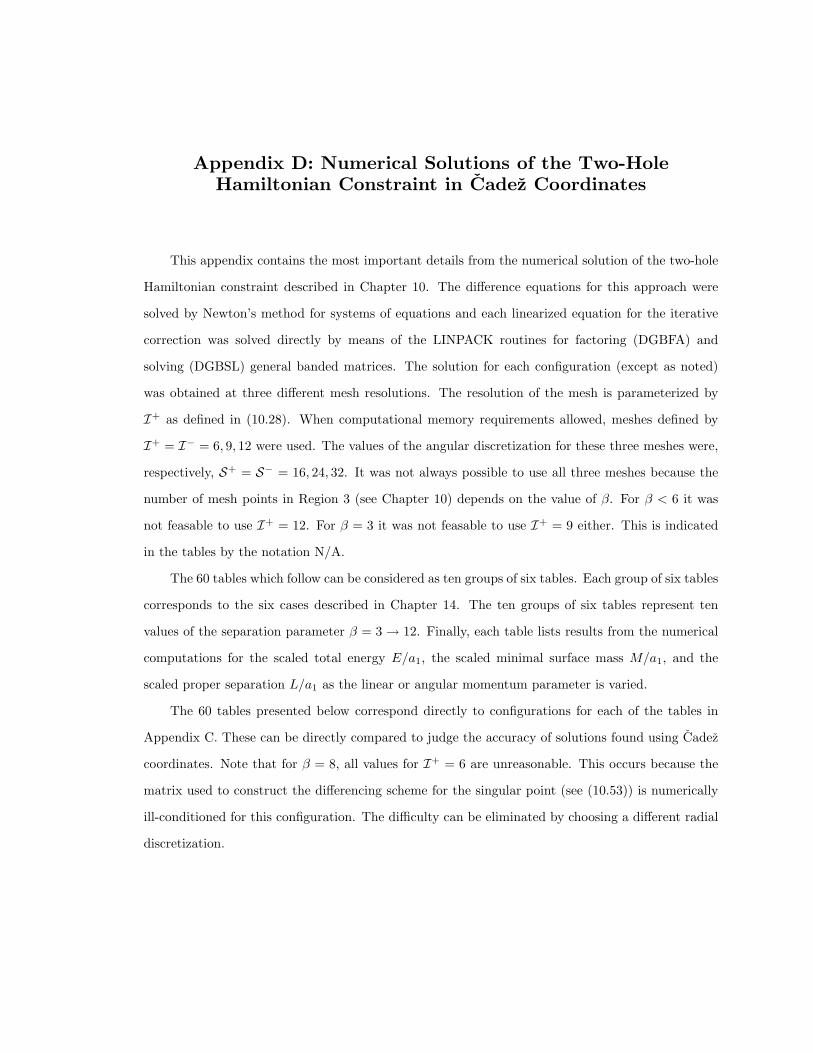
Appendix D: Numerical Solutions of the Two-HoleHamiltonian Constraint in Cadez Coordinates

This appendix contains the most important details from the numerical solution of the two-hole

Hamiltonian constraint described in Chapter 10. The difference equations for this approach were

solved by Newton’s method for systems of equations and each linearized equation for the iterative

correction was solved directly by means of the LINPACK routines for factoring (DGBFA) and

solving (DGBSL) general banded matrices. The solution for each configuration (except as noted)

was obtained at three different mesh resolutions. The resolution of the mesh is parameterized by

I+ as defined in (10.28). When computational memory requirements allowed, meshes defined by

I+ = I− = 6, 9, 12 were used. The values of the angular discretization for these three meshes were,

respectively, S+ = S− = 16, 24, 32. It was not always possible to use all three meshes because the

number of mesh points in Region 3 (see Chapter 10) depends on the value of β. For β < 6 it was

not feasable to use I+ = 12. For β = 3 it was not feasable to use I+ = 9 either. This is indicated

in the tables by the notation N/A.

The 60 tables which follow can be considered as ten groups of six tables. Each group of six tables

corresponds to the six cases described in Chapter 14. The ten groups of six tables represent ten

values of the separation parameter β = 3→ 12. Finally, each table lists results from the numerical

computations for the scaled total energy E/a1, the scaled minimal surface mass M/a1, and the

scaled proper separation L/a1 as the linear or angular momentum parameter is varied.

The 60 tables presented below correspond directly to configurations for each of the tables in

Appendix C. These can be directly compared to judge the accuracy of solutions found using Cadez

coordinates. Note that for β = 8, all values for I+ = 6 are unreasonable. This occurs because the

matrix used to construct the differencing scheme for the singular point (see (10.53)) is numerically

ill-conditioned for this configuration. The difficulty can be eliminated by choosing a different radial

discretization.

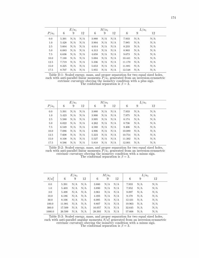
174

E/a1 M/a1 L/a1

P/a1 6 9 12 6 9 12 6 9 12

0.0 5.391 N/A N/A 3.880 N/A N/A 7.933 N/A N/A

1.0 5.428 N/A N/A 3.904 N/A N/A 7.985 N/A N/A

2.5 5.604 N/A N/A 4.014 N/A N/A 8.233 N/A N/A

5.0 6.083 N/A N/A 4.313 N/A N/A 8.903 N/A N/A

7.5 6.636 N/A N/A 4.658 N/A N/A 9.673 N/A N/A

10.0 7.188 N/A N/A 5.004 N/A N/A 10.441 N/A N/A

12.5 7.719 N/A N/A 5.336 N/A N/A 11.179 N/A N/A

15.0 8.225 N/A N/A 5.653 N/A N/A 11.881 N/A N/A

17.5 8.707 N/A N/A 5.955 N/A N/A 12.548 N/A N/A

Table D.1: Scaled energy, mass, and proper separation for two equal sized holes,each with anti-parallel linear momenta P/a1 generated from an inversion-symmetric

extrinsic curvature obeying the isometry condition with a plus sign.The conformal separation is β = 3.

E/a1 M/a1 L/a1

P/a1 6 9 12 6 9 12 6 9 12

0.0 5.391 N/A N/A 3.880 N/A N/A 7.933 N/A N/A

1.0 5.423 N/A N/A 3.900 N/A N/A 7.975 N/A N/A

2.5 5.580 N/A N/A 3.995 N/A N/A 8.174 N/A N/A

5.0 6.022 N/A N/A 4.262 N/A N/A 8.736 N/A N/A

7.5 6.549 N/A N/A 4.580 N/A N/A 9.406 N/A N/A

10.0 7.086 N/A N/A 4.906 N/A N/A 10.089 N/A N/A

12.5 7.608 N/A N/A 5.223 N/A N/A 10.754 N/A N/A

15.0 8.108 N/A N/A 5.527 N/A N/A 11.392 N/A N/A

17.5 8.586 N/A N/A 5.818 N/A N/A 12.001 N/A N/A

Table D.2: Scaled energy, mass, and proper separation for two equal sized holes,each with anti-parallel linear momenta P/a1 generated from an inversion-symmetric

extrinsic curvature obeying the isometry condition with a minus sign.The conformal separation is β = 3.

E/a1 M/a1 L/a1

S/a21 6 9 12 6 9 12 6 9 12

0.0 5.391 N/A N/A 3.880 N/A N/A 7.933 N/A N/A

1.0 5.403 N/A N/A 3.890 N/A N/A 7.952 N/A N/A

3.0 5.498 N/A N/A 3.961 N/A N/A 8.097 N/A N/A

10.0 6.186 N/A N/A 4.493 N/A N/A 9.178 N/A N/A

30.0 8.106 N/A N/A 6.095 N/A N/A 12.431 N/A N/A

100.0 11.981 N/A N/A 9.807 N/A N/A 19.963 N/A N/A

300.0 17.509 N/A N/A 16.057 N/A N/A 32.645 N/A N/A

1000.0 26.599 N/A N/A 28.393 N/A N/A 57.668 N/A N/A

Table D.3: Scaled energy, mass, and proper separation for two equal sized holes,each with anti-parallel angular momenta S/a2

1 generated from an inversion-symmetricextrinsic curvature obeying the isometry condition with a minus sign.

The conformal separation is β = 3.

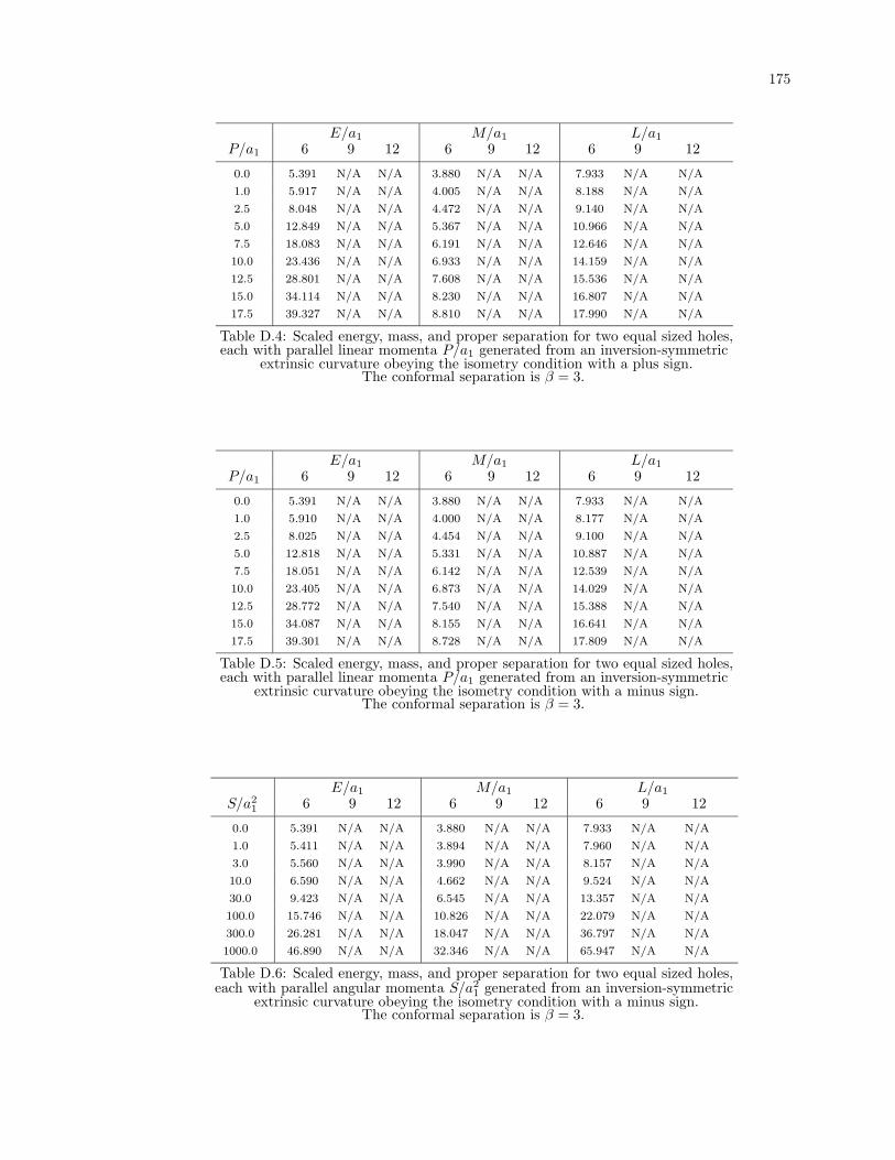
175

E/a1 M/a1 L/a1

P/a1 6 9 12 6 9 12 6 9 12

0.0 5.391 N/A N/A 3.880 N/A N/A 7.933 N/A N/A

1.0 5.917 N/A N/A 4.005 N/A N/A 8.188 N/A N/A

2.5 8.048 N/A N/A 4.472 N/A N/A 9.140 N/A N/A

5.0 12.849 N/A N/A 5.367 N/A N/A 10.966 N/A N/A

7.5 18.083 N/A N/A 6.191 N/A N/A 12.646 N/A N/A

10.0 23.436 N/A N/A 6.933 N/A N/A 14.159 N/A N/A

12.5 28.801 N/A N/A 7.608 N/A N/A 15.536 N/A N/A

15.0 34.114 N/A N/A 8.230 N/A N/A 16.807 N/A N/A

17.5 39.327 N/A N/A 8.810 N/A N/A 17.990 N/A N/A

Table D.4: Scaled energy, mass, and proper separation for two equal sized holes,each with parallel linear momenta P/a1 generated from an inversion-symmetric

extrinsic curvature obeying the isometry condition with a plus sign.The conformal separation is β = 3.

E/a1 M/a1 L/a1

P/a1 6 9 12 6 9 12 6 9 12

0.0 5.391 N/A N/A 3.880 N/A N/A 7.933 N/A N/A

1.0 5.910 N/A N/A 4.000 N/A N/A 8.177 N/A N/A

2.5 8.025 N/A N/A 4.454 N/A N/A 9.100 N/A N/A

5.0 12.818 N/A N/A 5.331 N/A N/A 10.887 N/A N/A

7.5 18.051 N/A N/A 6.142 N/A N/A 12.539 N/A N/A

10.0 23.405 N/A N/A 6.873 N/A N/A 14.029 N/A N/A

12.5 28.772 N/A N/A 7.540 N/A N/A 15.388 N/A N/A

15.0 34.087 N/A N/A 8.155 N/A N/A 16.641 N/A N/A

17.5 39.301 N/A N/A 8.728 N/A N/A 17.809 N/A N/A

Table D.5: Scaled energy, mass, and proper separation for two equal sized holes,each with parallel linear momenta P/a1 generated from an inversion-symmetric

extrinsic curvature obeying the isometry condition with a minus sign.The conformal separation is β = 3.

E/a1 M/a1 L/a1

S/a21 6 9 12 6 9 12 6 9 12

0.0 5.391 N/A N/A 3.880 N/A N/A 7.933 N/A N/A

1.0 5.411 N/A N/A 3.894 N/A N/A 7.960 N/A N/A

3.0 5.560 N/A N/A 3.990 N/A N/A 8.157 N/A N/A

10.0 6.590 N/A N/A 4.662 N/A N/A 9.524 N/A N/A

30.0 9.423 N/A N/A 6.545 N/A N/A 13.357 N/A N/A

100.0 15.746 N/A N/A 10.826 N/A N/A 22.079 N/A N/A

300.0 26.281 N/A N/A 18.047 N/A N/A 36.797 N/A N/A

1000.0 46.890 N/A N/A 32.346 N/A N/A 65.947 N/A N/A

Table D.6: Scaled energy, mass, and proper separation for two equal sized holes,each with parallel angular momenta S/a2

1 generated from an inversion-symmetricextrinsic curvature obeying the isometry condition with a minus sign.

The conformal separation is β = 3.

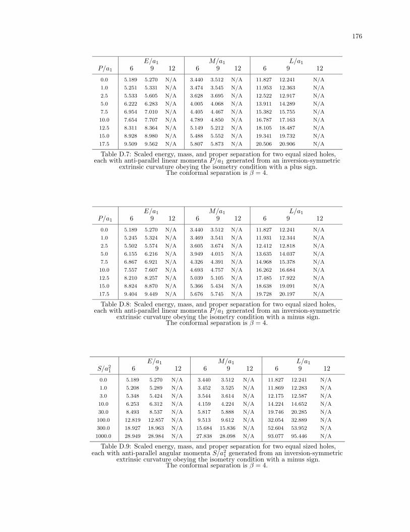
176

E/a1 M/a1 L/a1

P/a1 6 9 12 6 9 12 6 9 12

0.0 5.189 5.270 N/A 3.440 3.512 N/A 11.827 12.241 N/A

1.0 5.251 5.331 N/A 3.474 3.545 N/A 11.953 12.363 N/A

2.5 5.533 5.605 N/A 3.628 3.695 N/A 12.522 12.917 N/A

5.0 6.222 6.283 N/A 4.005 4.068 N/A 13.911 14.289 N/A

7.5 6.954 7.010 N/A 4.405 4.467 N/A 15.382 15.755 N/A

10.0 7.654 7.707 N/A 4.789 4.850 N/A 16.787 17.163 N/A

12.5 8.311 8.364 N/A 5.149 5.212 N/A 18.105 18.487 N/A

15.0 8.928 8.980 N/A 5.488 5.552 N/A 19.341 19.732 N/A

17.5 9.509 9.562 N/A 5.807 5.873 N/A 20.506 20.906 N/A

Table D.7: Scaled energy, mass, and proper separation for two equal sized holes,each with anti-parallel linear momenta P/a1 generated from an inversion-symmetric

extrinsic curvature obeying the isometry condition with a plus sign.The conformal separation is β = 4.

E/a1 M/a1 L/a1

P/a1 6 9 12 6 9 12 6 9 12

0.0 5.189 5.270 N/A 3.440 3.512 N/A 11.827 12.241 N/A

1.0 5.245 5.324 N/A 3.469 3.541 N/A 11.931 12.344 N/A

2.5 5.502 5.574 N/A 3.605 3.674 N/A 12.412 12.818 N/A

5.0 6.155 6.216 N/A 3.949 4.015 N/A 13.635 14.037 N/A

7.5 6.867 6.921 N/A 4.326 4.391 N/A 14.968 15.378 N/A

10.0 7.557 7.607 N/A 4.693 4.757 N/A 16.262 16.684 N/A

12.5 8.210 8.257 N/A 5.039 5.105 N/A 17.485 17.922 N/A

15.0 8.824 8.870 N/A 5.366 5.434 N/A 18.638 19.091 N/A

17.5 9.404 9.449 N/A 5.676 5.745 N/A 19.728 20.197 N/A

Table D.8: Scaled energy, mass, and proper separation for two equal sized holes,each with anti-parallel linear momenta P/a1 generated from an inversion-symmetric

extrinsic curvature obeying the isometry condition with a minus sign.The conformal separation is β = 4.

E/a1 M/a1 L/a1

S/a21 6 9 12 6 9 12 6 9 12

0.0 5.189 5.270 N/A 3.440 3.512 N/A 11.827 12.241 N/A

1.0 5.208 5.289 N/A 3.452 3.525 N/A 11.869 12.283 N/A

3.0 5.348 5.424 N/A 3.544 3.614 N/A 12.175 12.587 N/A

10.0 6.253 6.312 N/A 4.159 4.224 N/A 14.224 14.652 N/A

30.0 8.493 8.537 N/A 5.817 5.888 N/A 19.746 20.285 N/A

100.0 12.819 12.857 N/A 9.513 9.612 N/A 32.054 32.889 N/A

300.0 18.927 18.963 N/A 15.684 15.836 N/A 52.604 53.952 N/A

1000.0 28.949 28.984 N/A 27.838 28.098 N/A 93.077 95.446 N/A

Table D.9: Scaled energy, mass, and proper separation for two equal sized holes,each with anti-parallel angular momenta S/a2

1 generated from an inversion-symmetricextrinsic curvature obeying the isometry condition with a minus sign.

The conformal separation is β = 4.

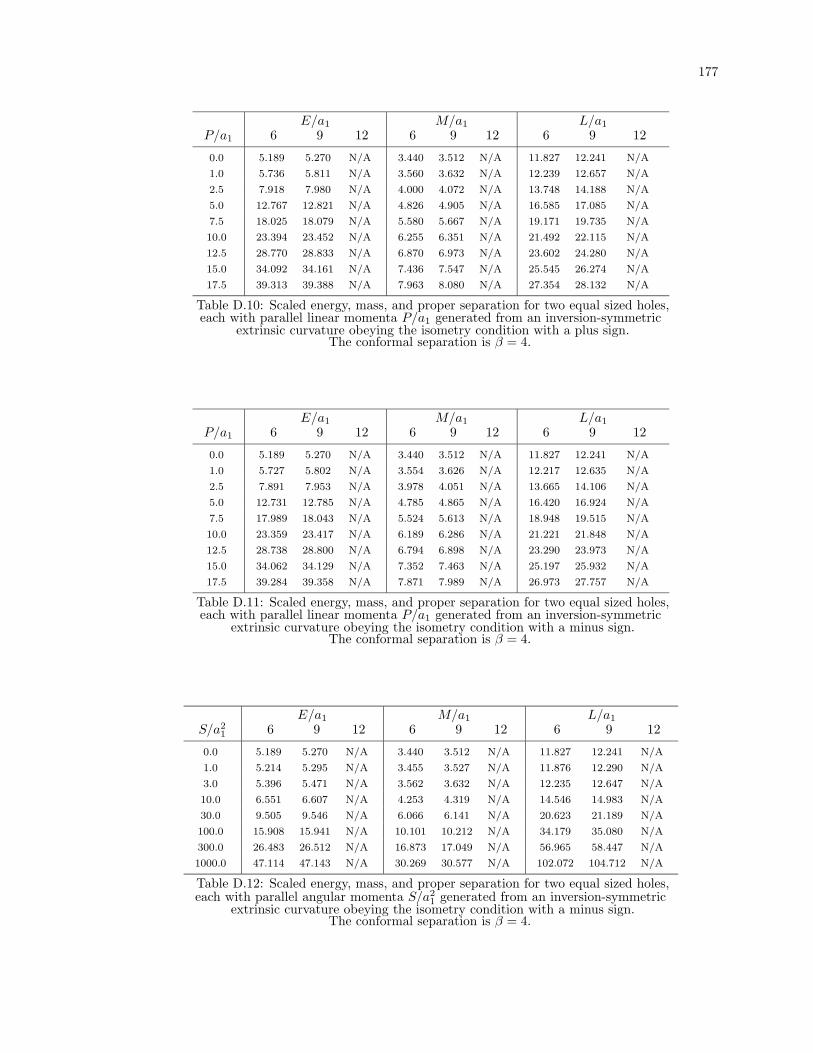
177

E/a1 M/a1 L/a1

P/a1 6 9 12 6 9 12 6 9 12

0.0 5.189 5.270 N/A 3.440 3.512 N/A 11.827 12.241 N/A

1.0 5.736 5.811 N/A 3.560 3.632 N/A 12.239 12.657 N/A

2.5 7.918 7.980 N/A 4.000 4.072 N/A 13.748 14.188 N/A

5.0 12.767 12.821 N/A 4.826 4.905 N/A 16.585 17.085 N/A

7.5 18.025 18.079 N/A 5.580 5.667 N/A 19.171 19.735 N/A

10.0 23.394 23.452 N/A 6.255 6.351 N/A 21.492 22.115 N/A

12.5 28.770 28.833 N/A 6.870 6.973 N/A 23.602 24.280 N/A

15.0 34.092 34.161 N/A 7.436 7.547 N/A 25.545 26.274 N/A

17.5 39.313 39.388 N/A 7.963 8.080 N/A 27.354 28.132 N/A

Table D.10: Scaled energy, mass, and proper separation for two equal sized holes,each with parallel linear momenta P/a1 generated from an inversion-symmetric

extrinsic curvature obeying the isometry condition with a plus sign.The conformal separation is β = 4.

E/a1 M/a1 L/a1

P/a1 6 9 12 6 9 12 6 9 12

0.0 5.189 5.270 N/A 3.440 3.512 N/A 11.827 12.241 N/A

1.0 5.727 5.802 N/A 3.554 3.626 N/A 12.217 12.635 N/A

2.5 7.891 7.953 N/A 3.978 4.051 N/A 13.665 14.106 N/A

5.0 12.731 12.785 N/A 4.785 4.865 N/A 16.420 16.924 N/A

7.5 17.989 18.043 N/A 5.524 5.613 N/A 18.948 19.515 N/A

10.0 23.359 23.417 N/A 6.189 6.286 N/A 21.221 21.848 N/A

12.5 28.738 28.800 N/A 6.794 6.898 N/A 23.290 23.973 N/A

15.0 34.062 34.129 N/A 7.352 7.463 N/A 25.197 25.932 N/A

17.5 39.284 39.358 N/A 7.871 7.989 N/A 26.973 27.757 N/A

Table D.11: Scaled energy, mass, and proper separation for two equal sized holes,each with parallel linear momenta P/a1 generated from an inversion-symmetric

extrinsic curvature obeying the isometry condition with a minus sign.The conformal separation is β = 4.

E/a1 M/a1 L/a1

S/a21 6 9 12 6 9 12 6 9 12

0.0 5.189 5.270 N/A 3.440 3.512 N/A 11.827 12.241 N/A

1.0 5.214 5.295 N/A 3.455 3.527 N/A 11.876 12.290 N/A

3.0 5.396 5.471 N/A 3.562 3.632 N/A 12.235 12.647 N/A

10.0 6.551 6.607 N/A 4.253 4.319 N/A 14.546 14.983 N/A

30.0 9.505 9.546 N/A 6.066 6.141 N/A 20.623 21.189 N/A

100.0 15.908 15.941 N/A 10.101 10.212 N/A 34.179 35.080 N/A

300.0 26.483 26.512 N/A 16.873 17.049 N/A 56.965 58.447 N/A

1000.0 47.114 47.143 N/A 30.269 30.577 N/A 102.072 104.712 N/A

Table D.12: Scaled energy, mass, and proper separation for two equal sized holes,each with parallel angular momenta S/a2

1 generated from an inversion-symmetricextrinsic curvature obeying the isometry condition with a minus sign.

The conformal separation is β = 4.

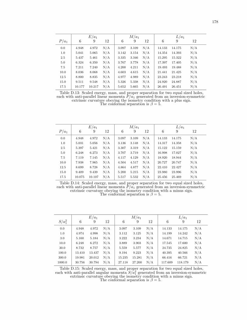
178

E/a1 M/a1 L/a1

P/a1 6 9 12 6 9 12 6 9 12

0.0 4.948 4.972 N/A 3.097 3.109 N/A 14.133 14.175 N/A

1.0 5.041 5.065 N/A 3.142 3.154 N/A 14.354 14.393 N/A

2.5 5.437 5.461 N/A 3.335 3.346 N/A 15.295 15.322 N/A

5.0 6.324 6.350 N/A 3.767 3.778 N/A 17.397 17.405 N/A

7.5 7.211 7.240 N/A 4.200 4.211 N/A 19.493 19.488 N/A

10.0 8.036 8.068 N/A 4.603 4.615 N/A 21.441 21.425 N/A

12.5 8.800 8.835 N/A 4.977 4.989 N/A 23.243 23.218 N/A

15.0 9.511 9.548 N/A 5.326 5.338 N/A 24.920 24.887 N/A

17.5 10.177 10.217 N/A 5.652 5.665 N/A 26.491 26.451 N/A

Table D.13: Scaled energy, mass, and proper separation for two equal sized holes,each with anti-parallel linear momenta P/a1 generated from an inversion-symmetric

extrinsic curvature obeying the isometry condition with a plus sign.The conformal separation is β = 5.

E/a1 M/a1 L/a1

P/a1 6 9 12 6 9 12 6 9 12

0.0 4.948 4.972 N/A 3.097 3.109 N/A 14.133 14.175 N/A

1.0 5.031 5.056 N/A 3.136 3.148 N/A 14.317 14.358 N/A

2.5 5.397 5.421 N/A 3.307 3.319 N/A 15.122 15.159 N/A

5.0 6.248 6.273 N/A 3.707 3.719 N/A 16.998 17.027 N/A

7.5 7.119 7.145 N/A 4.117 4.129 N/A 18.920 18.944 N/A

10.0 7.938 7.965 N/A 4.504 4.517 N/A 20.727 20.747 N/A

12.5 8.699 8.728 N/A 4.864 4.877 N/A 22.410 22.427 N/A

15.0 9.409 9.439 N/A 5.200 5.215 N/A 23.980 23.996 N/A

17.5 10.075 10.107 N/A 5.517 5.532 N/A 25.456 25.469 N/A

Table D.14: Scaled energy, mass, and proper separation for two equal sized holes,each with anti-parallel linear momenta P/a1 generated from an inversion-symmetric

extrinsic curvature obeying the isometry condition with a minus sign.The conformal separation is β = 5.

E/a1 M/a1 L/a1

S/a21 6 9 12 6 9 12 6 9 12

0.0 4.948 4.972 N/A 3.097 3.109 N/A 14.133 14.175 N/A

1.0 4.974 4.998 N/A 3.112 3.125 N/A 14.199 14.242 N/A

3.0 5.160 5.184 N/A 3.222 3.234 N/A 14.671 14.715 N/A

10.0 6.248 6.272 N/A 3.889 3.903 N/A 17.545 17.600 N/A

30.0 8.732 8.757 N/A 5.559 5.577 N/A 24.735 24.825 N/A

100.0 13.410 13.437 N/A 9.194 9.223 N/A 40.395 40.566 N/A

300.0 19.981 20.012 N/A 15.235 15.281 N/A 66.416 66.721 N/A

1000.0 30.756 30.794 N/A 27.118 27.200 N/A 117.609 118.179 N/A

Table D.15: Scaled energy, mass, and proper separation for two equal sized holes,each with anti-parallel angular momenta S/a2

1 generated from an inversion-symmetricextrinsic curvature obeying the isometry condition with a minus sign.

The conformal separation is β = 5.

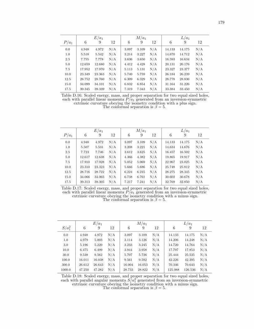
179

E/a1 M/a1 L/a1

P/a1 6 9 12 6 9 12 6 9 12

0.0 4.948 4.972 N/A 3.097 3.109 N/A 14.133 14.175 N/A

1.0 5.518 5.542 N/A 3.214 3.227 N/A 14.670 14.712 N/A

2.5 7.755 7.778 N/A 3.636 3.650 N/A 16.593 16.634 N/A

5.0 12.659 12.680 N/A 4.412 4.428 N/A 20.131 20.176 N/A

7.5 17.952 17.970 N/A 5.113 5.131 N/A 23.327 23.377 N/A

10.0 23.349 23.363 N/A 5.740 5.759 N/A 26.184 26.239 N/A

12.5 28.752 28.760 N/A 6.309 6.329 N/A 28.778 28.836 N/A

15.0 34.099 34.101 N/A 6.832 6.854 N/A 31.164 31.226 N/A

17.5 39.345 39.339 N/A 7.319 7.343 N/A 33.384 33.450 N/A

Table D.16: Scaled energy, mass, and proper separation for two equal sized holes,each with parallel linear momenta P/a1 generated from an inversion-symmetric

extrinsic curvature obeying the isometry condition with a plus sign.The conformal separation is β = 5.

E/a1 M/a1 L/a1

P/a1 6 9 12 6 9 12 6 9 12

0.0 4.948 4.972 N/A 3.097 3.109 N/A 14.133 14.175 N/A

1.0 5.507 5.531 N/A 3.208 3.221 N/A 14.634 14.676 N/A

2.5 7.723 7.746 N/A 3.612 3.625 N/A 16.457 16.502 N/A

5.0 12.617 12.638 N/A 4.366 4.382 N/A 19.865 19.917 N/A

7.5 17.910 17.928 N/A 5.052 5.069 N/A 22.967 23.025 N/A

10.0 23.310 23.323 N/A 5.666 5.686 N/A 25.748 25.812 N/A

12.5 28.716 28.722 N/A 6.224 6.245 N/A 28.275 28.345 N/A

15.0 34.066 34.065 N/A 6.738 6.761 N/A 30.602 30.678 N/A

17.5 39.313 39.305 N/A 7.217 7.241 N/A 32.769 32.850 N/A

Table D.17: Scaled energy, mass, and proper separation for two equal sized holes,each with parallel linear momenta P/a1 generated from an inversion-symmetric

extrinsic curvature obeying the isometry condition with a minus sign.The conformal separation is β = 5.

E/a1 M/a1 L/a1

S/a21 6 9 12 6 9 12 6 9 12

0.0 4.948 4.972 N/A 3.097 3.109 N/A 14.133 14.175 N/A

1.0 4.979 5.003 N/A 3.114 3.126 N/A 14.206 14.248 N/A

3.0 5.196 5.220 N/A 3.233 3.245 N/A 14.720 14.764 N/A

10.0 6.475 6.499 N/A 3.944 3.958 N/A 17.797 17.853 N/A

30.0 9.538 9.562 N/A 5.707 5.726 N/A 25.444 25.535 N/A

100.0 16.011 16.038 N/A 9.561 9.592 N/A 42.226 42.395 N/A

300.0 26.612 26.643 N/A 16.004 16.053 N/A 70.346 70.643 N/A

1000.0 47.250 47.282 N/A 28.733 28.822 N/A 125.988 126.536 N/A

Table D.18: Scaled energy, mass, and proper separation for two equal sized holes,each with parallel angular momenta S/a2

1 generated from an inversion-symmetricextrinsic curvature obeying the isometry condition with a minus sign.

The conformal separation is β = 5.

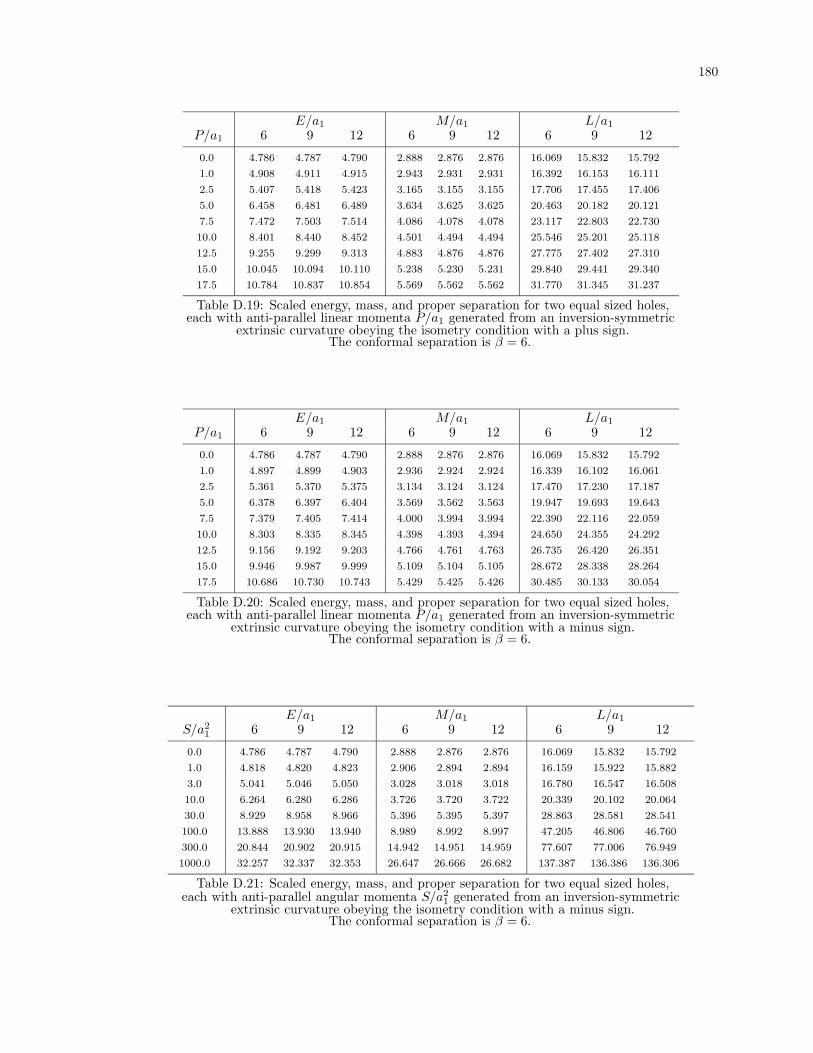
180

E/a1 M/a1 L/a1

P/a1 6 9 12 6 9 12 6 9 12

0.0 4.786 4.787 4.790 2.888 2.876 2.876 16.069 15.832 15.792

1.0 4.908 4.911 4.915 2.943 2.931 2.931 16.392 16.153 16.111

2.5 5.407 5.418 5.423 3.165 3.155 3.155 17.706 17.455 17.406

5.0 6.458 6.481 6.489 3.634 3.625 3.625 20.463 20.182 20.121

7.5 7.472 7.503 7.514 4.086 4.078 4.078 23.117 22.803 22.730

10.0 8.401 8.440 8.452 4.501 4.494 4.494 25.546 25.201 25.118

12.5 9.255 9.299 9.313 4.883 4.876 4.876 27.775 27.402 27.310

15.0 10.045 10.094 10.110 5.238 5.230 5.231 29.840 29.441 29.340

17.5 10.784 10.837 10.854 5.569 5.562 5.562 31.770 31.345 31.237

Table D.19: Scaled energy, mass, and proper separation for two equal sized holes,each with anti-parallel linear momenta P/a1 generated from an inversion-symmetric

extrinsic curvature obeying the isometry condition with a plus sign.The conformal separation is β = 6.

E/a1 M/a1 L/a1

P/a1 6 9 12 6 9 12 6 9 12

0.0 4.786 4.787 4.790 2.888 2.876 2.876 16.069 15.832 15.792

1.0 4.897 4.899 4.903 2.936 2.924 2.924 16.339 16.102 16.061

2.5 5.361 5.370 5.375 3.134 3.124 3.124 17.470 17.230 17.187

5.0 6.378 6.397 6.404 3.569 3.562 3.563 19.947 19.693 19.643

7.5 7.379 7.405 7.414 4.000 3.994 3.994 22.390 22.116 22.059

10.0 8.303 8.335 8.345 4.398 4.393 4.394 24.650 24.355 24.292

12.5 9.156 9.192 9.203 4.766 4.761 4.763 26.735 26.420 26.351

15.0 9.946 9.987 9.999 5.109 5.104 5.105 28.672 28.338 28.264

17.5 10.686 10.730 10.743 5.429 5.425 5.426 30.485 30.133 30.054

Table D.20: Scaled energy, mass, and proper separation for two equal sized holes,each with anti-parallel linear momenta P/a1 generated from an inversion-symmetric

extrinsic curvature obeying the isometry condition with a minus sign.The conformal separation is β = 6.

E/a1 M/a1 L/a1

S/a21 6 9 12 6 9 12 6 9 12

0.0 4.786 4.787 4.790 2.888 2.876 2.876 16.069 15.832 15.792

1.0 4.818 4.820 4.823 2.906 2.894 2.894 16.159 15.922 15.882

3.0 5.041 5.046 5.050 3.028 3.018 3.018 16.780 16.547 16.508

10.0 6.264 6.280 6.286 3.726 3.720 3.722 20.339 20.102 20.064

30.0 8.929 8.958 8.966 5.396 5.395 5.397 28.863 28.581 28.541

100.0 13.888 13.930 13.940 8.989 8.992 8.997 47.205 46.806 46.760

300.0 20.844 20.902 20.915 14.942 14.951 14.959 77.607 77.006 76.949

1000.0 32.257 32.337 32.353 26.647 26.666 26.682 137.387 136.386 136.306

Table D.21: Scaled energy, mass, and proper separation for two equal sized holes,each with anti-parallel angular momenta S/a2

1 generated from an inversion-symmetricextrinsic curvature obeying the isometry condition with a minus sign.

The conformal separation is β = 6.

181

E/a1 M/a1 L/a1

P/a1 6 9 12 6 9 12 6 9 12

0.0 4.786 4.787 4.790 2.888 2.876 2.876 16.069 15.832 15.792

1.0 5.370 5.375 5.380 3.004 2.993 2.993 16.714 16.473 16.432

2.5 7.636 7.653 7.659 3.414 3.404 3.405 18.987 18.729 18.683

5.0 12.559 12.590 12.599 4.157 4.148 4.149 23.115 22.814 22.759

7.5 17.854 17.895 17.906 4.825 4.816 4.817 26.822 26.480 26.417

10.0 23.248 23.296 23.309 5.420 5.411 5.412 30.130 29.749 29.678

12.5 28.644 28.697 28.713 5.960 5.950 5.952 33.128 32.712 32.634

15.0 33.983 34.042 34.058 6.457 6.446 6.448 35.886 35.437 35.352

17.5 39.220 39.282 39.300 6.918 6.908 6.909 38.451 37.971 37.880

Table D.22: Scaled energy, mass, and proper separation for two equal sized holes,each with parallel linear momenta P/a1 generated from an inversion-symmetric

extrinsic curvature obeying the isometry condition with a plus sign.The conformal separation is β = 6.

E/a1 M/a1 L/a1

P/a1 6 9 12 6 9 12 6 9 12

0.0 4.786 4.787 4.790 2.888 2.876 2.876 16.069 15.832 15.792

1.0 5.357 5.362 5.366 2.997 2.986 2.986 16.662 16.423 16.383

2.5 7.600 7.616 7.622 3.387 3.377 3.378 18.797 18.545 18.502

5.0 12.513 12.542 12.551 4.107 4.098 4.099 22.746 22.459 22.409

7.5 17.809 17.847 17.858 4.758 4.749 4.751 26.322 25.999 25.942

10.0 23.206 23.251 23.264 5.340 5.331 5.333 29.523 29.166 29.103

12.5 28.605 28.656 28.670 5.868 5.860 5.861 32.430 32.041 31.973

15.0 33.948 34.003 34.018 6.355 6.346 6.348 35.106 34.688 34.614

17.5 39.188 39.246 39.262 6.807 6.798 6.800 37.597 37.151 37.073

Table D.23: Scaled energy, mass, and proper separation for two equal sized holes,each with parallel linear momenta P/a1 generated from an inversion-symmetric

extrinsic curvature obeying the isometry condition with a minus sign.The conformal separation is β = 6.

E/a1 M/a1 L/a1

S/a21 6 9 12 6 9 12 6 9 12

0.0 4.786 4.787 4.790 2.888 2.876 2.876 16.069 15.832 15.792

1.0 4.822 4.823 4.827 2.907 2.895 2.895 16.164 15.927 15.887

3.0 5.069 5.074 5.079 3.035 3.025 3.025 16.818 16.585 16.545

10.0 6.440 6.458 6.464 3.760 3.755 3.756 20.532 20.293 20.254

30.0 9.584 9.615 9.623 5.492 5.490 5.493 29.436 29.145 29.104

100.0 16.114 16.159 16.169 9.237 9.239 9.244 48.780 48.353 48.300

300.0 26.733 26.795 26.808 15.480 15.486 15.495 81.139 80.470 80.396

1000.0 47.353 47.438 47.455 27.806 27.821 27.837 145.168 144.011 143.891

Table D.24: Scaled energy, mass, and proper separation for two equal sized holes,each with parallel angular momenta S/a2

1 generated from an inversion-symmetricextrinsic curvature obeying the isometry condition with a minus sign.

The conformal separation is β = 6.

182

E/a1 M/a1 L/a1

P/a1 6 9 12 6 9 12 6 9 12

0.0 4.706 4.674 4.667 2.789 2.741 2.728 18.384 17.603 17.364

1.0 4.851 4.827 4.821 2.850 2.804 2.791 18.808 18.028 17.788

2.5 5.426 5.425 5.426 3.090 3.049 3.038 20.480 19.690 19.440

5.0 6.597 6.628 6.639 3.580 3.544 3.535 23.874 23.023 22.745

7.5 7.708 7.759 7.777 4.045 4.011 4.001 27.080 26.152 25.844

10.0 8.719 8.785 8.808 4.468 4.435 4.425 29.994 28.990 28.652

12.5 9.644 9.723 9.750 4.856 4.823 4.813 32.659 31.582 31.217

15.0 10.500 10.589 10.619 5.215 5.181 5.172 35.122 33.977 33.586

17.5 11.299 11.396 11.430 5.550 5.516 5.506 37.421 36.210 35.795

Table D.25: Scaled energy, mass, and proper separation for two equal sized holes,each with anti-parallel linear momenta P/a1 generated from an inversion-symmetric

extrinsic curvature obeying the isometry condition with a plus sign.The conformal separation is β = 7.

E/a1 M/a1 L/a1

P/a1 6 9 12 6 9 12 6 9 12

0.0 4.706 4.674 4.667 2.789 2.741 2.728 18.384 17.603 17.364

1.0 4.837 4.813 4.807 2.841 2.795 2.783 18.736 17.960 17.722

2.5 5.376 5.373 5.373 3.056 3.016 3.005 20.175 19.404 19.164

5.0 6.515 6.541 6.550 3.513 3.479 3.470 23.225 22.423 22.168

7.5 7.616 7.660 7.675 3.955 3.924 3.915 26.176 25.321 25.045

10.0 8.625 8.683 8.702 4.361 4.331 4.323 28.884 27.972 27.674

12.5 9.552 9.619 9.642 4.735 4.705 4.697 31.372 30.405 30.086

15.0 10.410 10.486 10.511 5.081 5.052 5.044 33.679 32.657 32.319

17.5 11.211 11.294 11.322 5.406 5.376 5.368 35.836 34.762 34.406

Table D.26: Scaled energy, mass, and proper separation for two equal sized holes,each with anti-parallel linear momenta P/a1 generated from an inversion-symmetric

extrinsic curvature obeying the isometry condition with a minus sign.The conformal separation is β = 7.

E/a1 M/a1 L/a1

S/a21 6 9 12 6 9 12 6 9 12

0.0 4.706 4.674 4.667 2.789 2.741 2.728 18.384 17.603 17.364

1.0 4.742 4.712 4.705 2.807 2.760 2.747 18.493 17.713 17.475

3.0 4.985 4.968 4.964 2.935 2.893 2.881 19.244 18.471 18.234

10.0 6.286 6.305 6.311 3.645 3.613 3.605 23.415 22.599 22.348

30.0 9.071 9.125 9.142 5.312 5.285 5.279 33.218 32.186 31.869

100.0 14.240 14.335 14.363 8.880 8.851 8.845 54.204 52.646 52.172

300.0 21.502 21.642 21.682 14.786 14.749 14.742 88.954 86.505 85.765

1000.0 33.435 33.639 33.696 26.395 26.341 26.331 157.271 153.063 151.799

Table D.27: Scaled energy, mass, and proper separation for two equal sized holes,each with anti-parallel angular momenta S/a2

1 generated from an inversion-symmetricextrinsic curvature obeying the isometry condition with a minus sign.

The conformal separation is β = 7.

183

E/a1 M/a1 L/a1

P/a1 6 9 12 6 9 12 6 9 12

0.0 4.706 4.674 4.667 2.789 2.741 2.728 18.384 17.603 17.364

1.0 5.291 5.272 5.268 2.902 2.856 2.844 19.128 18.340 18.098

2.5 7.558 7.566 7.574 3.301 3.258 3.247 21.745 20.908 20.648

5.0 12.482 12.509 12.531 4.022 3.980 3.969 26.482 25.518 25.215

7.5 17.782 17.806 17.842 4.669 4.624 4.613 30.734 29.640 29.295

10.0 23.186 23.195 23.243 5.246 5.198 5.186 34.525 33.312 32.927

12.5 28.595 28.583 28.643 5.768 5.718 5.705 37.961 36.637 36.217

15.0 33.949 33.912 33.983 6.249 6.196 6.182 41.122 39.695 39.241

17.5 39.203 39.137 39.219 6.696 6.641 6.626 44.061 42.538 42.052

Table D.28: Scaled energy, mass, and proper separation for two equal sized holes,each with parallel linear momenta P/a1 generated from an inversion-symmetric

extrinsic curvature obeying the isometry condition with a plus sign.The conformal separation is β = 7.

E/a1 M/a1 L/a1

P/a1 6 9 12 6 9 12 6 9 12

0.0 4.706 4.674 4.667 2.789 2.741 2.728 18.384 17.603 17.364

1.0 5.277 5.257 5.253 2.894 2.848 2.836 19.061 18.275 18.035

2.5 7.519 7.525 7.532 3.271 3.229 3.218 21.495 20.672 20.418

5.0 12.434 12.457 12.479 3.967 3.926 3.915 25.997 25.063 24.773

7.5 17.737 17.756 17.790 4.597 4.553 4.542 30.075 29.026 28.698

10.0 23.145 23.148 23.194 5.159 5.114 5.102 33.726 32.567 32.205

12.5 28.559 28.540 28.597 5.670 5.622 5.609 37.042 35.782 35.387

15.0 33.917 33.872 33.941 6.140 6.089 6.076 40.096 38.740 38.316

17.5 39.174 39.101 39.180 6.578 6.524 6.510 42.938 41.493 41.040

Table D.29: Scaled energy, mass, and proper separation for two equal sized holes,each with parallel linear momenta P/a1 generated from an inversion-symmetric

extrinsic curvature obeying the isometry condition with a minus sign.The conformal separation is β = 7.

E/a1 M/a1 L/a1

S/a21 6 9 12 6 9 12 6 9 12

0.0 4.706 4.674 4.667 2.789 2.741 2.728 18.384 17.603 17.364

1.0 4.744 4.715 4.708 2.808 2.761 2.748 18.497 17.717 17.479

3.0 5.007 4.990 4.987 2.940 2.897 2.886 19.273 18.500 18.263

10.0 6.425 6.445 6.452 3.668 3.636 3.628 23.570 22.748 22.495

30.0 9.611 9.670 9.687 5.379 5.351 5.344 33.701 32.649 32.326

100.0 16.163 16.267 16.297 9.060 9.028 9.021 55.615 53.996 53.501

300.0 26.772 26.923 26.968 15.188 15.145 15.136 92.258 89.658 88.869

1000.0 47.345 47.549 47.617 27.284 27.215 27.201 164.789 160.227 158.847

Table D.30: Scaled energy, mass, and proper separation for two equal sized holes,each with parallel angular momenta S/a2

1 generated from an inversion-symmetricextrinsic curvature obeying the isometry condition with a minus sign.

The conformal separation is β = 7.

184

E/a1 M/a1 L/a1

P/a1 6 9 12 6 9 12 6 9 12

0.0 9.740 4.407 4.524 12.155 2.434 2.563 248.286 15.837 17.803

1.0 9.746 4.627 4.717 12.160 2.513 2.635 248.380 16.347 18.313

2.5 9.776 5.421 5.440 12.184 2.797 2.905 248.869 18.208 20.222

5.0 9.881 6.883 6.822 12.269 3.326 3.422 250.570 21.689 23.880

7.5 10.047 8.197 8.087 12.404 3.805 3.899 253.268 24.853 27.243

10.0 10.264 9.365 9.222 12.580 4.234 4.327 256.796 27.687 30.268

12.5 10.522 10.421 10.253 12.788 4.623 4.718 260.979 30.260 33.021

15.0 10.812 11.390 11.202 13.021 4.981 5.078 265.653 32.628 35.558

17.5 11.124 12.290 12.084 13.272 5.315 5.413 270.682 34.831 37.921

Table D.31: Scaled energy, mass, and proper separation for two equal sized holes,each with anti-parallel linear momenta P/a1 generated from an inversion-symmetric

extrinsic curvature obeying the isometry condition with a plus sign.The conformal separation is β = 8.

E/a1 M/a1 L/a1

P/a1 6 9 12 6 9 12 6 9 12

0.0 9.740 4.407 4.524 12.155 2.434 2.563 248.286 15.837 17.803

1.0 9.746 4.608 4.700 12.159 2.505 2.626 248.370 16.300 18.245

2.5 9.774 5.355 5.380 12.181 2.767 2.872 248.804 18.030 19.957

5.0 9.873 6.773 6.724 12.257 3.269 3.360 250.321 21.332 23.354

7.5 10.030 8.066 7.975 12.379 3.729 3.816 252.739 24.361 26.527

10.0 10.238 9.222 9.103 12.539 4.143 4.230 255.922 27.083 29.400

12.5 10.487 10.270 10.130 12.729 4.520 4.607 259.721 29.559 32.023

15.0 10.767 11.233 11.076 12.944 4.868 4.956 263.997 31.841 34.444

17.5 11.070 12.129 11.957 13.177 5.191 5.281 268.628 33.965 36.702

Table D.32: Scaled energy, mass, and proper separation for two equal sized holes,each with anti-parallel linear momenta P/a1 generated from an inversion-symmetric

extrinsic curvature obeying the isometry condition with a minus sign.The conformal separation is β = 8.

E/a1 M/a1 L/a1

S/a21 6 9 12 6 9 12 6 9 12

0.0 9.740 4.407 4.524 12.155 2.434 2.563 248.286 15.837 17.803

1.0 9.741 4.460 4.570 12.156 2.459 2.585 248.300 15.976 17.936

3.0 9.745 4.803 4.873 12.161 2.620 2.732 248.412 16.873 18.824

10.0 9.792 6.378 6.352 12.225 3.395 3.483 249.659 21.224 23.354

30.0 10.149 9.460 9.346 12.715 5.075 5.159 259.244 30.704 33.490

100.0 12.142 15.035 14.820 15.541 8.594 8.696 314.451 50.652 54.939

300.0 16.575 22.811 22.487 22.335 14.391 14.533 446.800 83.584 90.383

1000.0 25.028 35.555 35.076 36.951 25.775 26.000 730.809 148.301 160.046

Table D.33: Scaled energy, mass, and proper separation for two equal sized holes,each with anti-parallel angular momenta S/a2

1 generated from an inversion-symmetricextrinsic curvature obeying the isometry condition with a minus sign.

The conformal separation is β = 8.

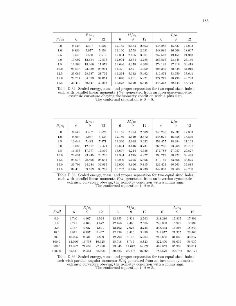
185

E/a1 M/a1 L/a1

P/a1 6 9 12 6 9 12 6 9 12

0.0 9.740 4.407 4.524 12.155 2.434 2.563 248.286 15.837 17.803

1.0 9.889 5.077 5.153 12.190 2.558 2.681 248.989 16.606 18.607

2.5 10.646 7.538 7.519 12.364 2.965 3.081 252.523 19.151 21.340

5.0 13.092 12.654 12.533 12.904 3.664 3.785 263.516 23.545 26.150

7.5 16.563 18.060 17.872 13.626 4.278 4.408 278.181 27.416 30.418

10.0 20.648 23.532 23.291 14.421 4.821 4.962 294.339 30.848 34.210

12.5 25.086 28.987 28.702 15.234 5.312 5.462 310.874 33.950 37.641

15.0 29.714 34.373 34.051 16.040 5.761 5.921 327.272 36.798 40.793

17.5 34.419 39.647 39.293 16.828 6.179 6.348 343.313 39.444 43.722

Table D.34: Scaled energy, mass, and proper separation for two equal sized holes,each with parallel linear momenta P/a1 generated from an inversion-symmetric

extrinsic curvature obeying the isometry condition with a plus sign.The conformal separation is β = 8.

E/a1 M/a1 L/a1

P/a1 6 9 12 6 9 12 6 9 12

0.0 9.740 4.407 4.524 12.155 2.434 2.563 248.286 15.837 17.803

1.0 9.889 5.057 5.135 12.189 2.549 2.672 248.977 16.558 18.540

2.5 10.644 7.483 7.471 12.360 2.938 3.052 252.457 18.994 21.103

5.0 13.086 12.577 12.471 12.894 3.616 3.731 263.298 23.268 25.707

7.5 16.553 17.977 17.809 13.607 4.214 4.338 277.788 27.057 29.827

10.0 20.637 23.445 23.230 14.394 4.745 4.877 293.779 30.422 33.498

12.5 25.076 28.898 28.644 15.200 5.225 5.366 310.162 33.466 36.825

15.0 29.704 34.284 33.995 16.000 5.666 5.815 326.422 36.263 39.885

17.5 34.410 39.559 39.239 16.782 6.075 6.233 342.337 38.863 42.730

Table D.35: Scaled energy, mass, and proper separation for two equal sized holes,each with parallel linear momenta P/a1 generated from an inversion-symmetric

extrinsic curvature obeying the isometry condition with a minus sign.The conformal separation is β = 8.

E/a1 M/a1 L/a1

S/a21 6 9 12 6 9 12 6 9 12

0.0 9.740 4.407 4.524 12.155 2.434 2.563 248.286 15.837 17.803

1.0 9.741 4.463 4.572 12.156 2.460 2.585 248.303 15.979 17.939

3.0 9.747 4.822 4.891 12.162 2.623 2.735 248.432 16.893 18.845

10.0 9.811 6.497 6.467 12.236 3.410 3.499 249.877 21.325 23.464

30.0 10.295 9.931 9.809 12.793 5.118 5.204 260.858 31.030 33.847

100.0 13.056 16.758 16.525 15.918 8.716 8.823 322.400 51.636 56.030

300.0 19.892 27.639 27.280 23.345 14.672 14.827 468.859 85.938 93.017

1000.0 35.541 48.551 48.008 39.423 26.407 26.665 786.576 153.742 166.179

Table D.36: Scaled energy, mass, and proper separation for two equal sized holes,each with parallel angular momenta S/a2

1 generated from an inversion-symmetricextrinsic curvature obeying the isometry condition with a minus sign.

The conformal separation is β = 8.

186

E/a1 M/a1 L/a1

P/a1 6 9 12 6 9 12 6 9 12

0.0 4.359 4.456 4.480 2.389 2.489 2.513 17.843 19.309 19.649

1.0 4.600 4.676 4.695 2.472 2.567 2.589 18.473 19.924 20.261

2.5 5.456 5.475 5.483 2.769 2.851 2.871 20.711 22.166 22.506

5.0 7.007 6.967 6.963 3.308 3.383 3.402 24.793 26.352 26.720

7.5 8.394 8.320 8.308 3.793 3.867 3.885 28.462 30.155 30.556

10.0 9.626 9.528 9.512 4.225 4.300 4.319 31.735 33.559 33.994

12.5 10.740 10.624 10.604 4.617 4.694 4.713 34.700 36.651 37.117

15.0 11.761 11.631 11.609 4.978 5.056 5.076 37.426 39.496 39.992

17.5 12.710 12.568 12.543 5.313 5.394 5.414 39.962 42.144 42.669

Table D.37: Scaled energy, mass, and proper separation for two equal sized holes,each with anti-parallel linear momenta P/a1 generated from an inversion-symmetric

extrinsic curvature obeying the isometry condition with a plus sign.The conformal separation is β = 9.

E/a1 M/a1 L/a1

P/a1 6 9 12 6 9 12 6 9 12

0.0 4.359 4.456 4.480 2.389 2.489 2.513 17.843 19.309 19.649

1.0 4.580 4.657 4.676 2.463 2.558 2.580 18.398 19.840 20.176

2.5 5.389 5.413 5.421 2.735 2.817 2.837 20.435 21.846 22.177

5.0 6.903 6.870 6.867 3.246 3.319 3.337 24.262 25.727 26.073

7.5 8.275 8.210 8.200 3.711 3.782 3.800 27.747 29.309 29.680

10.0 9.499 9.414 9.400 4.129 4.200 4.218 30.870 32.536 32.934

12.5 10.608 10.508 10.490 4.508 4.580 4.599 33.706 35.475 35.898

15.0 11.627 11.514 11.494 4.857 4.931 4.950 36.318 38.186 38.633

17.5 12.573 12.450 12.428 5.183 5.258 5.277 38.749 40.711 41.182

Table D.38: Scaled energy, mass, and proper separation for two equal sized holes,each with anti-parallel linear momenta P/a1 generated from an inversion-symmetric

extrinsic curvature obeying the isometry condition with a minus sign.The conformal separation is β = 9.

E/a1 M/a1 L/a1

S/a21 6 9 12 6 9 12 6 9 12

0.0 4.359 4.456 4.480 2.389 2.489 2.513 17.843 19.309 19.649

1.0 4.415 4.506 4.529 2.414 2.512 2.535 17.998 19.460 19.799

3.0 4.772 4.832 4.847 2.577 2.665 2.686 18.998 20.450 20.787

10.0 6.397 6.381 6.380 3.353 3.424 3.441 23.786 25.384 25.752

30.0 9.571 9.481 9.464 5.025 5.096 5.112 34.158 36.280 36.767

100.0 15.325 15.147 15.112 8.525 8.613 8.634 55.961 59.274 60.036

300.0 23.373 23.094 23.040 14.290 14.414 14.444 91.958 97.258 98.479

1000.0 36.581 36.161 36.078 25.608 25.807 25.857 162.708 171.916 174.041

Table D.39: Scaled energy, mass, and proper separation for two equal sized holes,each with anti-parallel angular momenta S/a2

1 generated from an inversion-symmetricextrinsic curvature obeying the isometry condition with a minus sign.

The conformal separation is β = 9.

187

E/a1 M/a1 L/a1

P/a1 6 9 12 6 9 12 6 9 12

0.0 4.359 4.456 4.480 2.389 2.489 2.513 17.843 19.309 19.649

1.0 5.029 5.092 5.109 2.511 2.607 2.629 18.719 20.197 20.539

2.5 7.486 7.471 7.475 2.913 3.003 3.024 21.612 23.192 23.556

5.0 12.599 12.490 12.486 3.602 3.694 3.716 26.596 28.438 28.860

7.5 18.009 17.827 17.824 4.206 4.304 4.328 30.983 33.085 33.564

10.0 23.489 23.242 23.245 4.740 4.846 4.871 34.869 37.210 37.744

12.5 28.956 28.648 28.659 5.222 5.335 5.362 38.382 40.942 41.526

15.0 34.357 33.990 34.012 5.665 5.785 5.814 41.606 44.370 45.000

17.5 39.647 39.227 39.259 6.075 6.202 6.233 44.602 47.557 48.229

Table D.40: Scaled energy, mass, and proper separation for two equal sized holes,each with parallel linear momenta P/a1 generated from an inversion-symmetric

extrinsic curvature obeying the isometry condition with a plus sign.The conformal separation is β = 9.

E/a1 M/a1 L/a1

P/a1 6 9 12 6 9 12 6 9 12

0.0 4.359 4.456 4.480 2.389 2.489 2.513 17.843 19.309 19.649

1.0 5.008 5.073 5.091 2.502 2.597 2.620 18.647 20.115 20.456

2.5 7.431 7.420 7.425 2.882 2.971 2.992 21.369 22.909 23.266

5.0 12.526 12.425 12.423 3.547 3.637 3.659 26.150 27.909 28.315

7.5 17.932 17.763 17.762 4.134 4.230 4.253 30.392 32.378 32.836

10.0 23.412 23.180 23.186 4.655 4.758 4.783 34.161 36.360 36.867

12.5 28.880 28.589 28.603 5.126 5.235 5.262 37.573 39.969 40.520

15.0 34.283 33.935 33.959 5.558 5.674 5.702 40.707 43.287 43.880

17.5 39.575 39.174 39.209 5.959 6.082 6.112 43.622 46.373 47.006

Table D.41: Scaled energy, mass, and proper separation for two equal sized holes,each with parallel linear momenta P/a1 generated from an inversion-symmetric

extrinsic curvature obeying the isometry condition with a minus sign.The conformal separation is β = 9.

E/a1 M/a1 L/a1

S/a21 6 9 12 6 9 12 6 9 12

0.0 4.359 4.456 4.480 2.389 2.489 2.513 17.843 19.309 19.649

1.0 4.417 4.508 4.530 2.415 2.513 2.536 18.001 19.462 19.801

3.0 4.787 4.846 4.862 2.579 2.667 2.688 19.014 20.467 20.804

10.0 6.494 6.476 6.474 3.364 3.435 3.452 23.868 25.472 25.841

30.0 9.971 9.875 9.857 5.058 5.129 5.146 34.441 36.582 37.074

100.0 16.848 16.654 16.616 8.619 8.710 8.733 56.872 60.250 61.027

300.0 27.761 27.452 27.393 14.511 14.645 14.678 94.239 99.709 100.970

1000.0 48.689 48.199 48.114 26.120 26.342 26.397 168.158 177.796 180.020

Table D.42: Scaled energy, mass, and proper separation for two equal sized holes,each with parallel angular momenta S/a2

1 generated from an inversion-symmetricextrinsic curvature obeying the isometry condition with a minus sign.

The conformal separation is β = 9.

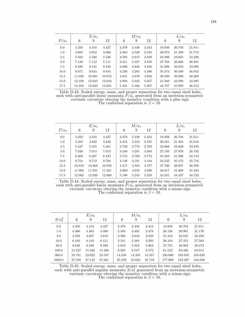
188

E/a1 M/a1 L/a1

P/a1 6 9 12 6 9 12 6 9 12

0.0 4.350 4.410 4.427 2.378 2.438 2.454 19.956 20.794 21.011

1.0 4.605 4.652 4.666 2.464 2.520 2.535 20.673 21.499 21.712

2.5 5.504 5.520 5.526 2.765 2.815 2.829 23.206 24.025 24.236

5.0 7.129 7.112 7.111 3.311 3.357 3.370 27.794 28.666 28.891

7.5 8.580 8.545 8.540 3.800 3.846 3.858 31.908 32.852 33.095

10.0 9.871 9.824 9.816 4.236 4.282 4.296 35.574 36.590 36.852

12.5 11.038 10.981 10.972 4.631 4.678 4.692 38.896 39.980 40.260

15.0 12.109 12.045 12.034 4.994 5.043 5.057 41.949 43.098 43.395

17.5 13.103 13.033 13.021 5.331 5.382 5.397 44.787 45.999 46.312

Table D.43: Scaled energy, mass, and proper separation for two equal sized holes,each with anti-parallel linear momenta P/a1 generated from an inversion-symmetric

extrinsic curvature obeying the isometry condition with a plus sign.The conformal separation is β = 10.

E/a1 M/a1 L/a1

P/a1 6 9 12 6 9 12 6 9 12

0.0 4.350 4.410 4.427 2.378 2.438 2.454 19.956 20.794 21.011

1.0 4.584 4.632 4.646 2.454 2.510 2.525 20.581 21.404 21.616

2.5 5.437 5.455 5.461 2.730 2.779 2.793 22.868 23.669 23.876

5.0 7.028 7.014 7.013 3.246 3.291 3.304 27.150 27.978 28.192

7.5 8.469 8.437 8.432 3.715 3.760 3.772 31.043 31.926 32.154

10.0 9.754 9.712 9.704 4.136 4.181 4.194 34.532 35.472 35.716

12.5 10.919 10.868 10.859 4.517 4.564 4.577 37.700 38.697 38.956

15.0 11.988 11.931 11.921 4.869 4.916 4.930 40.617 41.669 41.943

17.5 12.982 12.920 12.908 5.196 5.245 5.259 43.331 44.437 44.724

Table D.44: Scaled energy, mass, and proper separation for two equal sized holes,each with anti-parallel linear momenta P/a1 generated from an inversion-symmetric

extrinsic curvature obeying the isometry condition with a minus sign.The conformal separation is β = 10.

E/a1 M/a1 L/a1

S/a21 6 9 12 6 9 12 6 9 12

0.0 4.350 4.410 4.427 2.378 2.438 2.454 19.956 20.794 21.011

1.0 4.406 4.463 4.480 2.404 2.462 2.478 20.126 20.961 21.176

3.0 4.768 4.807 4.818 2.566 2.618 2.633 21.218 22.045 22.258

10.0 6.416 6.410 6.411 3.341 3.384 3.395 26.444 27.351 27.582

30.0 9.646 9.598 9.588 5.010 5.053 5.064 37.755 38.963 39.272

100.0 15.527 15.428 15.406 8.503 8.557 8.572 61.532 63.426 63.914

300.0 23.781 23.622 23.587 14.258 14.335 14.357 100.800 103.835 104.620

1000.0 37.358 37.116 37.061 25.558 25.683 25.718 177.989 183.267 184.638

Table D.45: Scaled energy, mass, and proper separation for two equal sized holes,each with anti-parallel angular momenta S/a2

1 generated from an inversion-symmetricextrinsic curvature obeying the isometry condition with a minus sign.

The conformal separation is β = 10.

189

E/a1 M/a1 L/a1

P/a1 6 9 12 6 9 12 6 9 12

0.0 4.350 4.410 4.427 2.378 2.438 2.454 19.956 20.794 21.011

1.0 5.010 5.051 5.063 2.498 2.555 2.570 20.916 21.756 21.973

2.5 7.443 7.439 7.439 2.893 2.946 2.961 24.104 24.990 25.216

5.0 12.524 12.468 12.452 3.573 3.628 3.643 29.615 30.637 30.896

7.5 17.911 17.815 17.785 4.171 4.229 4.245 34.475 35.635 35.929

10.0 23.371 23.240 23.196 4.699 4.762 4.779 38.785 40.072 40.398

12.5 28.822 28.658 28.599 5.176 5.243 5.262 42.681 44.086 44.442

15.0 34.208 34.012 33.940 5.614 5.686 5.705 46.258 47.774 48.158

17.5 39.485 39.260 39.174 6.021 6.096 6.117 49.583 51.201 51.611

Table D.46: Scaled energy, mass, and proper separation for two equal sized holes,each with parallel linear momenta P/a1 generated from an inversion-symmetric

extrinsic curvature obeying the isometry condition with a plus sign.The conformal separation is β = 10.

E/a1 M/a1 L/a1

P/a1 6 9 12 6 9 12 6 9 12

0.0 4.350 4.410 4.427 2.378 2.438 2.454 19.956 20.794 21.011

1.0 4.989 5.031 5.043 2.488 2.545 2.560 20.827 21.664 21.880

2.5 7.387 7.386 7.386 2.861 2.914 2.928 23.801 24.670 24.894

5.0 12.454 12.402 12.386 3.515 3.569 3.585 29.057 30.042 30.294

7.5 17.840 17.750 17.720 4.095 4.153 4.169 33.735 34.842 35.125

10.0 23.302 23.178 23.135 4.609 4.671 4.689 37.896 39.120 39.432

12.5 28.755 28.599 28.541 5.075 5.141 5.159 41.664 42.996 43.336

15.0 34.144 33.957 33.885 5.502 5.572 5.592 45.128 46.561 46.926

17.5 39.424 39.208 39.123 5.899 5.973 5.993 48.349 49.876 50.266

Table D.47: Scaled energy, mass, and proper separation for two equal sized holes,each with parallel linear momenta P/a1 generated from an inversion-symmetric

extrinsic curvature obeying the isometry condition with a minus sign.The conformal separation is β = 10.

E/a1 M/a1 L/a1

S/a21 6 9 12 6 9 12 6 9 12

0.0 4.350 4.410 4.427 2.378 2.438 2.454 19.956 20.794 21.011

1.0 4.408 4.465 4.481 2.404 2.462 2.478 20.127 20.963 21.178

3.0 4.780 4.818 4.830 2.568 2.620 2.634 21.231 22.058 22.271

10.0 6.496 6.489 6.489 3.349 3.392 3.403 26.513 27.422 27.654

30.0 9.988 9.937 9.926 5.035 5.078 5.090 38.004 39.221 39.533

100.0 16.877 16.769 16.745 8.578 8.634 8.650 62.380 64.303 64.798

300.0 27.781 27.606 27.565 14.440 14.522 14.545 103.001 106.116 106.921

1000.0 48.654 48.373 48.304 25.987 26.124 26.163 183.403 188.889 190.310

Table D.48: Scaled energy, mass, and proper separation for two equal sized holes,each with parallel angular momenta S/a2

1 generated from an inversion-symmetricextrinsic curvature obeying the isometry condition with a minus sign.

The conformal separation is β = 10.

190

E/a1 M/a1 L/a1

P/a1 6 9 12 6 9 12 6 9 12

0.0 4.319 4.369 4.384 2.345 2.392 2.406 21.502 22.139 22.310

1.0 4.594 4.633 4.645 2.434 2.478 2.491 22.304 22.928 23.095

2.5 5.550 5.565 5.570 2.742 2.782 2.793 25.100 25.712 25.875

5.0 7.263 7.253 7.253 3.295 3.332 3.343 30.117 30.762 30.933

7.5 8.788 8.764 8.761 3.788 3.825 3.836 34.596 35.292 35.475

10.0 10.142 10.110 10.105 4.226 4.264 4.276 38.583 39.329 39.526

12.5 11.365 11.327 11.321 4.623 4.662 4.674 42.192 42.987 43.197

15.0 12.488 12.445 12.437 4.987 5.028 5.041 45.509 46.350 46.573

17.5 13.530 13.483 13.475 5.326 5.369 5.382 48.592 49.478 49.712

Table D.49: Scaled energy, mass, and proper separation for two equal sized holes,each with anti-parallel linear momenta P/a1 generated from an inversion-symmetric

extrinsic curvature obeying the isometry condition with a plus sign.The conformal separation is β = 11.

E/a1 M/a1 L/a1

P/a1 6 9 12 6 9 12 6 9 12

0.0 4.319 4.369 4.384 2.345 2.392 2.406 21.502 22.139 22.310

1.0 4.571 4.611 4.624 2.423 2.468 2.481 22.200 22.823 22.990

2.5 5.482 5.498 5.504 2.706 2.745 2.757 24.726 25.328 25.489

5.0 7.163 7.154 7.154 3.229 3.265 3.277 29.411 30.030 30.195

7.5 8.678 8.656 8.653 3.702 3.738 3.750 33.653 34.310 34.485

10.0 10.028 9.998 9.993 4.124 4.162 4.174 37.447 38.147 38.333

12.5 11.250 11.215 11.208 4.508 4.547 4.559 40.892 41.633 41.830

15.0 12.373 12.333 12.325 4.861 4.901 4.914 44.061 44.843 45.051

17.5 13.415 13.371 13.363 5.189 5.231 5.244 47.011 47.831 48.049

Talbe D50: Scaled energy, mass, and proper separation for two equal sized holes,each with anti-parallel linear momenta P/a1 generated from an inversion-symmetric

extrinsic curvature obeying the isometry condition with a minus sign.The conformal separation is β = 11.

E/a1 M/a1 L/a1

S/a21 6 9 12 6 9 12 6 9 12

0.0 4.319 4.369 4.384 2.345 2.392 2.406 21.502 22.139 22.310

1.0 4.378 4.425 4.439 2.371 2.417 2.430 21.686 22.320 22.490

3.0 4.753 4.785 4.795 2.536 2.577 2.589 22.866 23.489 23.656

10.0 6.442 6.439 6.440 3.314 3.348 3.358 28.439 29.119 29.299

30.0 9.742 9.707 9.699 4.981 5.015 5.025 40.436 41.343 41.584

100.0 15.765 15.689 15.672 8.465 8.509 8.522 65.636 67.059 67.441

300.0 24.237 24.115 24.086 14.205 14.267 14.286 107.259 109.539 110.155

1000.0 38.199 38.011 37.966 25.475 25.576 25.607 189.090 193.055 194.132

Table D.51: Scaled energy, mass, and proper separation for two equal sized holes,each with anti-parallel angular momenta S/a2

1 generated from an inversion-symmetricextrinsic curvature obeying the isometry condition with a minus sign.

The conformal separation is β = 11.

191

E/a1 M/a1 L/a1

P/a1 6 9 12 6 9 12 6 9 12

0.0 4.319 4.369 4.384 2.345 2.392 2.406 21.502 22.139 22.310

1.0 4.981 5.016 5.026 2.464 2.509 2.522 22.534 23.168 23.338

2.5 7.417 7.420 7.415 2.855 2.897 2.910 25.953 26.615 26.790

5.0 12.503 12.476 12.441 3.527 3.571 3.584 31.862 32.618 32.817

7.5 17.896 17.855 17.785 4.117 4.164 4.178 37.074 37.929 38.153

10.0 23.365 23.315 23.206 4.639 4.690 4.704 41.696 42.644 42.891

12.5 28.826 28.770 28.619 5.111 5.165 5.180 45.875 46.910 47.179

15.0 34.224 34.164 33.969 5.543 5.600 5.617 49.714 50.829 51.118

17.5 39.513 39.451 39.213 5.945 6.005 6.023 53.281 54.471 54.779

Table D.52: Scaled energy, mass, and proper separation for two equal sized holes,each with parallel linear momenta P/a1 generated from an inversion-symmetric

extrinsic curvature obeying the isometry condition with a plus sign.The conformal separation is β = 11.

E/a1 M/a1 L/a1

P/a1 6 9 12 6 9 12 6 9 12

0.0 4.319 4.369 4.384 2.345 2.392 2.406 21.502 22.139 22.310

1.0 4.959 4.995 5.004 2.453 2.498 2.512 22.434 23.067 23.236

2.5 7.359 7.365 7.359 2.821 2.864 2.876 25.614 26.266 26.440

5.0 12.431 12.408 12.373 3.467 3.511 3.524 31.239 31.973 32.167

7.5 17.825 17.787 17.717 4.040 4.086 4.100 36.247 37.071 37.288

10.0 23.297 23.250 23.142 4.547 4.598 4.612 40.705 41.614 41.852

12.5 28.761 28.709 28.559 5.006 5.060 5.076 44.742 45.731 45.990

15.0 34.162 34.107 33.913 5.428 5.485 5.502 48.454 49.518 49.795

17.5 39.454 39.398 39.161 5.819 5.880 5.897 51.906 53.040 53.335

Table D.53: Scaled energy, mass, and proper separation for two equal sized holes,each with parallel linear momenta P/a1 generated from an inversion-symmetric

extrinsic curvature obeying the isometry condition with a minus sign.The conformal separation is β = 11.

E/a1 M/a1 L/a1

S/a21 6 9 12 6 9 12 6 9 12

0.0 4.319 4.369 4.384 2.345 2.392 2.406 21.502 22.139 22.310

1.0 4.380 4.426 4.440 2.371 2.417 2.430 21.688 22.321 22.491

3.0 4.763 4.794 4.804 2.537 2.578 2.591 22.876 23.500 23.666

10.0 6.509 6.506 6.506 3.320 3.354 3.364 28.496 29.177 29.358

30.0 10.038 10.001 9.993 5.000 5.035 5.045 40.653 41.565 41.807

100.0 16.973 16.892 16.872 8.525 8.570 8.584 66.407 67.847 68.233

300.0 27.909 27.776 27.741 14.355 14.420 14.440 109.327 111.657 112.286

1000.0 48.795 48.589 48.514 25.836 25.945 25.978 194.313 198.413 199.523

Table D.54: Scaled energy, mass, and proper separation for two equal sized holes,each with parallel angular momenta S/a2

1 generated from an inversion-symmetricextrinsic curvature obeying the isometry condition with a minus sign.

The conformal separation is β = 11.

192

E/a1 M/a1 L/a1

P/a1 6 9 12 6 9 12 6 9 12

0.0 4.288 4.334 4.348 2.311 2.353 2.366 22.890 23.429 23.578

1.0 4.583 4.618 4.629 2.403 2.443 2.455 23.771 24.297 24.441

2.5 5.596 5.609 5.615 2.718 2.754 2.764 26.812 27.322 27.460

5.0 7.394 7.387 7.388 3.277 3.310 3.321 32.218 32.750 32.893

7.5 8.991 8.972 8.971 3.773 3.807 3.817 37.029 37.599 37.751

10.0 10.407 10.381 10.378 4.213 4.248 4.260 41.305 41.916 42.077

12.5 11.686 11.655 11.651 4.612 4.648 4.660 45.175 45.824 45.996

15.0 12.859 12.825 12.819 4.977 5.015 5.027 48.730 49.416 49.598

17.5 13.948 13.911 13.905 5.317 5.357 5.369 52.035 52.756 52.947

Table D.55: Scaled energy, mass, and proper separation for two equal sized holes,each with anti-parallel linear momenta P/a1 generated from an inversion-symmetric

extrinsic curvature obeying the isometry condition with a plus sign.The conformal separation is β = 12.

E/a1 M/a1 L/a1

P/a1 6 9 12 6 9 12 6 9 12

0.0 4.288 4.334 4.348 2.311 2.353 2.366 22.890 23.429 23.578

1.0 4.559 4.595 4.607 2.392 2.432 2.444 23.658 24.184 24.328

2.5 5.526 5.541 5.546 2.681 2.717 2.728 26.410 26.914 27.051

5.0 7.294 7.288 7.288 3.210 3.244 3.254 31.467 31.982 32.121

7.5 8.882 8.864 8.862 3.686 3.720 3.731 36.029 36.574 36.720

10.0 10.295 10.271 10.267 4.111 4.146 4.157 40.104 40.683 40.838

12.5 11.573 11.544 11.539 4.496 4.533 4.544 43.801 44.413 44.577

15.0 12.746 12.714 12.708 4.850 4.888 4.900 47.202 47.847 48.019

17.5 13.836 13.801 13.794 5.180 5.219 5.232 50.366 51.042 51.223

Table D.56: Scaled energy, mass, and proper separation for two equal sized holes,each with anti-parallel linear momenta P/a1 generated from an inversion-symmetric

extrinsic curvature obeying the isometry condition with a minus sign.The conformal separation is β = 12.

E/a1 M/a1 L/a1

S/a21 6 9 12 6 9 12 6 9 12

0.0 4.288 4.334 4.348 2.311 2.353 2.366 22.890 23.429 23.578

1.0 4.350 4.393 4.406 2.338 2.379 2.391 23.088 23.624 23.771

3.0 4.738 4.767 4.776 2.506 2.543 2.554 24.347 24.871 25.014

10.0 6.468 6.466 6.467 3.288 3.318 3.327 30.224 30.790 30.943

30.0 9.835 9.805 9.799 4.953 4.983 4.993 42.807 43.560 43.764

100.0 15.992 15.928 15.912 8.430 8.468 8.480 69.214 70.394 70.718

300.0 24.673 24.569 24.543 14.155 14.210 14.228 112.838 114.729 115.251

1000.0 39.003 38.842 38.801 25.397 25.487 25.516 198.621 201.905 202.820

Table D.57: Scaled energy, mass, and proper separation for two equal sized holes,each with anti-parallel angular momenta S/a2

1 generated from an inversion-symmetricextrinsic curvature obeying the isometry condition with a minus sign.

The conformal separation is β = 12.

193

E/a1 M/a1 L/a1

P/a1 6 9 12 6 9 12 6 9 12

0.0 4.288 4.334 4.348 2.311 2.353 2.366 22.890 23.429 23.578

1.0 4.953 4.985 4.994 2.430 2.470 2.482 23.987 24.522 24.668

2.5 7.395 7.399 7.393 2.818 2.856 2.868 27.614 28.166 28.314

5.0 12.484 12.463 12.427 3.484 3.523 3.535 33.875 34.500 34.666

7.5 17.879 17.845 17.772 4.068 4.109 4.122 39.397 40.101 40.287

10.0 23.350 23.309 23.193 4.584 4.629 4.643 44.296 45.075 45.280

12.5 28.813 28.766 28.606 5.050 5.098 5.113 48.726 49.574 49.797

15.0 34.212 34.163 33.956 5.477 5.529 5.544 52.795 53.709 53.948

17.5 39.503 39.453 39.199 5.874 5.929 5.945 56.577 57.552 57.806

Table D.58: Scaled energy, mass, and proper separation for two equal sized holes,each with parallel linear momenta P/a1 generated from an inversion-symmetric

extrinsic curvature obeying the isometry condition with a plus sign.The conformal separation is β = 12.

E/a1 M/a1 L/a1

P/a1 6 9 12 6 9 12 6 9 12

0.0 4.288 4.334 4.348 2.311 2.353 2.366 22.890 23.429 23.578

1.0 4.930 4.963 4.972 2.419 2.459 2.472 23.878 24.412 24.558

2.5 7.336 7.341 7.335 2.784 2.822 2.833 27.246 27.792 27.940

5.0 12.411 12.392 12.356 3.423 3.462 3.474 33.201 33.812 33.976

7.5 17.807 17.776 17.702 3.988 4.031 4.044 38.505 39.188 39.370

10.0 23.281 23.243 23.127 4.490 4.535 4.549 43.227 43.979 44.179

12.5 28.747 28.705 28.544 4.943 4.992 5.007 47.504 48.322 48.538

15.0 34.150 34.105 33.898 5.360 5.412 5.427 51.438 52.316 52.548

17.5 39.445 39.398 39.145 5.747 5.801 5.818 55.096 56.032 56.279

Table D.59: Scaled energy, mass, and proper separation for two equal sized holes,each with parallel linear momenta P/a1 generated from an inversion-symmetric

extrinsic curvature obeying the isometry condition with a minus sign.The conformal separation is β = 12.

E/a1 M/a1 L/a1

S/a21 6 9 12 6 9 12 6 9 12

0.0 4.288 4.334 4.348 2.311 2.353 2.366 22.890 23.429 23.578

1.0 4.351 4.394 4.407 2.338 2.379 2.391 23.089 23.625 23.772

3.0 4.746 4.775 4.784 2.507 2.543 2.555 24.355 24.879 25.022

10.0 6.524 6.523 6.523 3.293 3.323 3.332 30.272 30.839 30.992

30.0 10.094 10.063 10.056 4.968 4.999 5.008 42.995 43.751 43.956

100.0 17.080 17.012 16.994 8.479 8.518 8.531 69.913 71.106 71.432

300.0 28.057 27.944 27.912 14.280 14.338 14.356 114.775 116.701 117.232

1000.0 48.968 48.791 48.720 25.704 25.800 25.831 203.634 207.018 207.956

Table D.60: Scaled energy, mass, and proper separation for two equal sized holes,each with parallel angular momenta S/a2

1 generated from an inversion-symmetricextrinsic curvature obeying the isometry condition with a minus sign.

The conformal separation is β = 12.

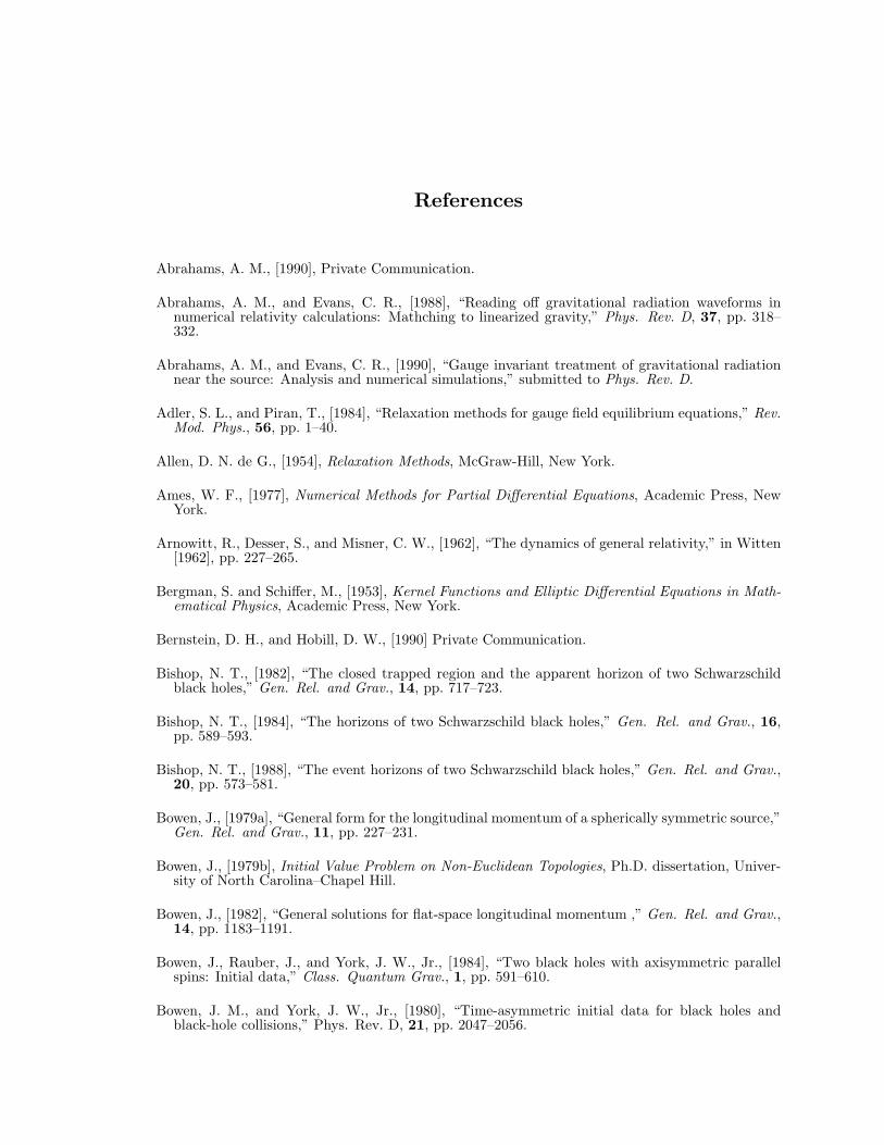
References

Abrahams, A. M., [1990], Private Communication.

Abrahams, A. M., and Evans, C. R., [1988], “Reading off gravitational radiation waveforms innumerical relativity calculations: Mathching to linearized gravity,” Phys. Rev. D, 37, pp. 318–332.

Abrahams, A. M., and Evans, C. R., [1990], “Gauge invariant treatment of gravitational radiationnear the source: Analysis and numerical simulations,” submitted to Phys. Rev. D.

Adler, S. L., and Piran, T., [1984], “Relaxation methods for gauge field equilibrium equations,” Rev.Mod. Phys., 56, pp. 1–40.

Allen, D. N. de G., [1954], Relaxation Methods, McGraw-Hill, New York.

Ames, W. F., [1977], Numerical Methods for Partial Differential Equations, Academic Press, NewYork.

Arnowitt, R., Desser, S., and Misner, C. W., [1962], “The dynamics of general relativity,” in Witten[1962], pp. 227–265.

Bergman, S. and Schiffer, M., [1953], Kernel Functions and Elliptic Differential Equations in Math-ematical Physics, Academic Press, New York.

Bernstein, D. H., and Hobill, D. W., [1990] Private Communication.

Bishop, N. T., [1982], “The closed trapped region and the apparent horizon of two Schwarzschildblack holes,” Gen. Rel. and Grav., 14, pp. 717–723.

Bishop, N. T., [1984], “The horizons of two Schwarzschild black holes,” Gen. Rel. and Grav., 16,pp. 589–593.

Bishop, N. T., [1988], “The event horizons of two Schwarzschild black holes,” Gen. Rel. and Grav.,20, pp. 573–581.

Bowen, J., [1979a], “General form for the longitudinal momentum of a spherically symmetric source,”Gen. Rel. and Grav., 11, pp. 227–231.

Bowen, J., [1979b], Initial Value Problem on Non-Euclidean Topologies, Ph.D. dissertation, Univer-sity of North Carolina–Chapel Hill.

Bowen, J., [1982], “General solutions for flat-space longitudinal momentum ,” Gen. Rel. and Grav.,14, pp. 1183–1191.

Bowen, J., Rauber, J., and York, J. W., Jr., [1984], “Two black holes with axisymmetric parallelspins: Initial data,” Class. Quantum Grav., 1, pp. 591–610.

Bowen, J. M., and York, J. W., Jr., [1980], “Time-asymmetric initial data for black holes andblack-hole collisions,” Phys. Rev. D, 21, pp. 2047–2056.

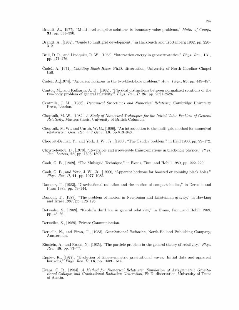
195

Brandt, A., [1977], “Multi-level adaptive solutions to boundary-value problems,” Math. of Comp.,31, pp. 333–390.

Brandt, A., [1982], “Guide to multigrid development,” in Hackbusch and Trottenberg 1982, pp. 220–312.

Brill, D. R., and Lindquist, R. W., [1963], “Interaction energy in geometrostatics,” Phys. Rev., 131,pp. 471–476.

Cadez, A.,[1971], Colliding Black Holes, Ph.D. dissertation, University of North Carolina–ChapelHill.

Cadez, A.,[1974], “Apparent horizons in the two-black-hole problem,” Ann. Phys., 83, pp. 449–457.

Cantor, M., and Kulkarni, A. D., [1982], “Physical distinctions between normalized solutions of thetwo-body problem of general relativity,” Phys. Rev. D, 25, pp. 2521–2526.

Centrella, J. M., [1986], Dynamical Spacetimes and Numerical Relativity, Cambridge UniversityPress, London.

Choptuik, M. W., [1982], A Study of Numerical Techniques for the Initial Value Problem of GeneralRelativity, Masters thesis, University of British Columbia.

Choptuik, M. W., and Unruh, W. G., [1986], “An introduction to the multi-grid method for numericalrelativists,” Gen. Rel. and Grav., 18, pp 813–843.

Choquet-Bruhat, Y., and York, J. W., Jr., [1980], “The Cauchy problem,” in Held 1980, pp. 99–172.

Christodoulou, D., [1970], “Reversible and irreversible transformations in black-hole physics,” Phys.Rev. Letters, 25, pp. 1596–1597.

Cook, G. B., [1989], “The Multigrid Technique,” in Evans, Finn, and Hobill 1989, pp. 222–229.

Cook, G. B., and York, J. W., Jr., [1990], “Apparent horizons for boosted or spinning black holes,”Phys. Rev. D, 41, pp. 1077–1085.

Damour, T., [1983], “Gravitational radiation and the motion of compact bodies,” in Deruelle andPiran 1983, pp. 59–144.

Damour, T., [1987], “The problem of motion in Newtonian and Einsteinian gravity,” in Hawkingand Israel 1987, pp. 128–198.

Detweiler, S., [1989], “Kepler’s third law in general relativity,” in Evans, Finn, and Hobill 1989,pp. 43–56.

Detweiler, S., [1989], Private Communication.

Deruelle, N., and Piran, T., [1983], Gravitational Radiation, North-Holland Publishing Company,Amsterdam.

Einstein, A., and Rosen, N., [1935], “The particle problem in the general theory of relativity,” Phys.Rev., 48, pp. 73–77.

Eppley, K., [1977], “Evolution of time-symmetric gravitational waves: Initial data and apparenthorizons,” Phys. Rev. D, 16, pp. 1609–1614.

Evans, C. R., [1984], A Method for Numerical Relativity: Simulation of Axisymmetric Gravita-tional Collapse and Gravitational Radiation Generation, Ph.D. dissertation, University of Texasat Austin.

196

Evans, C. R., [1986a], “An approach for calculating axisymmetric gravitational collapse,” in Centrella1986, pp. 3–39.

Evans, C. R., [1986b], Unpublished work.

Evans, C. R., [1987], “Gravitational radiation from collisions of compact stars,” in Ulmer 1987,pp. 152–156.

Evans, C. R., [1989], Private Communication.

Evans, C. R., Finn, L. S., and Hobill, D. W., [1989], Frontiers in Numerical Relativity, CambridgeUniversity Press, London.

Ferrell, R. C., and Eardley, D. M., [1989], “Slowly moving maximally charged black holes,” in Evans,Finn, and Hobill 1989, pp. 27–42.

Gibbons, G. W., [1972], “The time symmetric initial value problem for black holes,” Commun.Math. Phys., 27, pp. 87–102.

Gibbons, G. W., and Schutz, B. F., [1972], “Limits on gravitational radiation from two gravitation-ally bound black holes,” Mon. Not. R. Astr. Soc., 159, pp. 41P–45P.

Hackbusch, W., and Trottenberg, U., [1982], Multigrid Methods, Springer-Verlag, Berlin.

Hackbusch, W., [1985], Multi-Grid Methods and Applications, Springer-Verlag,Berlin.

Hahn, S., and Lindquist, R., [1964], “The two body problem in geometrodynamics,” Ann. Phys.,29, pp. 304–331.

Hawking, S. W., [1971], “Gravitational radiation from colliding black holes,” Phys. Rev. Letters,26, pp. 1344–1346.

Hawking, S. W., and Ellis, G. F. R., [1973], The Large Scale Structure of Space-Time, CambridgeUniversity Press, London.

Hawking, S. W., and Israel, W., [1987], 300 Years of Gravitation, Cambridge University Press,London.

Held, A., [1980], General Relativity and Gravitation: One Hundred Years After the Birth of AlbertEinstein, Volume 1, Plenum Press, London.

Jaffe, J., [1975], “The gravitational spin-spin force,” Gen. Rel. and Grav., 6, pp. 49–53.

Kulkarni, A. D., [1984], “Time-asymmetric initial data for the N black hole problem in generalrelativity,” J. Math. Phys., 25, pp. 1028–1034.

Kulkarni, A. D., Shepley, L. C., and York, J. W., Jr., [1983], “Initial data for N black holes,” Phys.Lett., 96A, pp. 228–230.

Lindquist, R. W., [1963], “Initial-value problems on Einstein-Rosen manifolds,” J. Math. Phys., 4,pp. 938–950.

Mashoon, B., [1971], “Particles with spin in a gravitational field,” J. Math. Phys., 12, pp. 1075–1077.

Matzner, R. and Shepley, L., [1982], Spacetime and Geometry: The Alfred Schild Lectures, Universityof Texas Press, Austin.

197

Misner, C. W., [1963], “The method of images in geometrostatics,” Ann. Phys., 24, pp. 102–117.

Misner, C. W., Thorne, K. S., and Wheeler, J. A., [1973], Gravitation, W. H. Freeman and Company,New York.

Mitchell, A. R., and Griffiths, D. F., [1980], The Finite Difference Method in Partial DifferentialEquations, John Wiley and Sons, New York.

Moon, P., and Spencer, D. E., [1988], Field Theory Handbook, Springer-Verlag, Berlin.

Nakamura, T., Kojima, Y., and Oohara, K., [1984], “A method of determining apparent horizons inthree-dimensional numerical relativity,” Phys. Lett., 106A, pp. 235–238.

Nakamura, T., Kojima, Y., and Oohara, K., [1985], “Apparent horizons of time-symmetric initialvalue for three black holes,” Phys. Lett., 107A, pp. 452–455.

Nakamura, T., and Oohara, K., [1989], “Methods in 3D numerical Relativity,” in Evans, Finn, andHobill 1989, pp. 254–280.

O Murchada, N., and York, J. W., Jr., [1973], “Existence and uniqueness of solutions of the Hamil-tonian constraint of general relativity on compact manifolds,” J. Math. Phys., 14, pp. 1551–1557.

O Murchada, N., and York, J. W., Jr., [1974a], “Initial-value problem of general relativity. I. Generalformulation and physical interpretation,” Phys. Rev. D, 10, pp. 428–436.

O Murchada, N., and York, J. W., Jr., [1974b], “Initial-value problem of general relativity. II.Stability of solution of the initial-value equations,” Phys. Rev. D, 10, pp. 437–446.

O Murchada, N., and York, J. W., Jr., [1974c], “Gravitational energy,” Phys. Rev. D, 10, pp. 2345–2357.

O Murchada, N., and York, J. W., Jr., [1976a], “Gravitational momentum,” unpublished.

O Murchada, N., and York, J. W., Jr., [1976b], “Gravitational potentials: A constructive approachto general relativity,” Gen. Rel. and Grav., 7, pp. 257–261.

Papagiannis, M. D., [1977], Eighth Texas Symposium on Relativistic Astrophysics, The New YorkAcademy of Sciences, New York.

Piran, T., [1988], Private Communication.

Piran, T., [1989], Private Communication.

Press, W. H., Flannery, B. P., Teukolky, S. A., and Vetterling, W. T., [1988], Numerical Recipes inC, Cambridge University Press, London.

Rauber, J. D., [1985], Initial Data for Black Hole Collisions, Ph.D. dissertation, University of NorthCarolina–Chapel Hill.

Rauber, J. D., [1986], “Initial data for black hole collisions,” in Centrella 1986, pp. 304–327.

Smarr, L. L., Cadez, A., DeWitt, W., Eppley, K., [1976], “Collision of two black holes: Theoreticalframework,” Phys. Rev. D, 14, pp. 2443–2452.

Smarr, L. L., [1977], “Space-times generated by computers: black holes with gravitational radiation”,in Papagiannis 1977, pp. 569–604.

198

Smarr, L. L., [1979], Sources of Gravitational Radiation, Cambridge University Press, London.

Smarr, L. L., and York, J. W., Jr., [1078a], “Radiation gauge in general relativity,” Phys. Rev. D,17, pp. 1945–1956.

Smarr, L. L., and York, J. W., Jr., [1078b], “Kinematical conditions in the construction of space-time,” Phys. Rev. D, 17, pp. 2529–2551.

Thornburg, J., [1987], “Coordinates and boundary conditions for the general relativistic initial dataproblem,” Class. Quantum Grav., 4, pp. 1119–11131.

Thorne, K. S., [1987], “Gravitational radiation,” in Hawking and Israel 1987, pp. 330–458.

Tipler, F. J., [1980], Essays in General Relativity, Academic Press, New York.

Tomimatsu, A., [1989], “Gravitational field in a collision of two Schwarzschild black holes,” Preprint.

Ulmer, M. P., [1987], Proceedings of the 13th Texas Symposium on Relativistic Astrophysics, WorldScientific Publishing, Singapore.

Wald, R. M., [1972], “Gravitational spin interaction,” Phys. Rev. D, 6, pp. 406–413.

Wald, R. M., [1984], General Relativity, The University of Chicago Press, Chicago.

Weinberg, S., [1972], Gravitation and Cosmology: Principles and Applications of the General Theoryof Relativity, Wiley and Sons, New York.

Witten, L., [1962], Gravitation: An Introduction to Current Research, John Wiley and Sons, NewYork.

York, J. W., Jr., [1971], “Gravitational degrees of freedom and the initial-value problem,” Phys.Rev. Letters, 26, pp. 1656–1658.

York, J. W., Jr., [1972], “Role of conformal three-geometry in the dynamics of gravitation,” Phys.Rev. Letters, 28, pp. 1082–1085.

York, J. W., Jr. [1973a], “Conformally invariant orthogonal decomposition of symmetric tensors onRiemannian manifolds and the initial-value problem of general relativity,” J. Math. Phys., 14,pp. 456–464.

York, J. W., Jr. [1973b], “Initial-value problem and dynamics of general relativity,” Lecture notes,Princeton University.

York, J. W., Jr. [1974], “Covariant decompositions of symmetric tensors in the theory of gravitation,”Ann. Inst. Henri Poincare, 21, pp. 319–332.

York, J. W., Jr., [1979], “Kinematics and Dynamics of General Relativity,” in Smarr 1979, pp. 83–126.

York, J. W., Jr., [1980], “Energy and momentum of the gravitational field,” in Tipler, pp. 39–58.

York, J. W., Jr., [1984], “Initial data for N black holes,” Physica, 124A, pp. 629–637.

York, J. W., Jr., [1989], “Initial data for collisions of black holes and other gravitational miscellany,”in Evans, Finn, and Hobill 1989, pp. 89–109.

York, J. W., Jr., and Piran, T., [1982], “The initial value problem and beyond,” in Matzner andShepley 1982, pp. 147–176.