Embed Size (px)
Citation preview
Institute of Mathematical StatisticsLECTURE NOTES-MONOGRAPH SERIES
Group Representations inProbability and Statistics
Persi DiaconisHarvard University

Institute of Mathematical Statistics
LECTURE NOTES-MONOGRAPH SERIESShanti S. Gupta, Series Editor
Volume 11
Group Representations inProbability and StatisticsPersi DiaconisHarvard University
Institute of Mathematical StatisticsHayward, California
Institute ofMathematical Statistics
Lecture Notes-Monograph Series
Series Editor, Shanti S. Gupta, Purdue University
The production of the [MS Lecture Notes-Monograph Series ismanaged by the IMS Business Office: Jessica Utts, IMSTreasurer, and Jose L. Gonzalez, IMS Business Manager.
Library of Congress Catalog Card Number: 88-82779
International Standard Book Number 0-940600-14-5
Copyright © 1988 Institute of Mathematical Statistics
All rights reserved
Printed in the United States of America

Table of Contents
Preface v
Chapter 1 - IntroductionA. Introduction 1B. Annotated bibliography 2
Chapter 2 - Basics of Representations and CharactersA. Definitions and examples 5B. The basic theorems 7C. Decomposition of the regular representation and Fourier 12
inversionD. Number of irreducible representations 14E. Products of Groups 16
Chapter 3 - Random Walks on GroupsA. Examples 17B. The basic setup 21C. Some explicit computations 25D. Random transpositions: an introduction to the representation 36
theory of the symmetric groupE. The Markov chain connection 48F. Random walks on homogeneous spaces and Gelfand pairs 51G. Some references 61H. First hitting times 64
Chapter 4 - Probabilistic ArgumentsA. Introduction - strong uniform times 69B. Examples of strong uniform times 72C. A closer look at strong uniform times 75D. An analysis of real riffle shuffles 77E. Coupling 84F. First hits and first time to cover all 87G. Some open problems on random walk and strong uniform times 89
Chapter 5 - Examples of Data on Permutations andHomogeneous Spaces
A. Permutation data 92B. Partially ranked data 93C. The d-sphere Sd 99D. Other groups 100
iii

IV
E. Statistics on groups 101
Chapter 6 - Metrics on Groups, and Their Statistical UsesA. Applications of metrics 102B. Some metrics on permutations 112C. General constructions of metrics 119D. Metrics on h·omogeneous spaces 124E. Some Philosophy 129
Chapter 7 - Representation Theory of the Symmetric GroupA. Construction of the irreducible representations of 131
the symmetric groupB. More on representations of Sn 136
Chapter 8 - Spectral AnalysisA. Data on groups 141B. Data on homogeneous spaces 147C. Analysis of variance 153D. Thoughts about spectral analysis 161
Chapter 9 - ModelsA. Exponential families from representations 167B. Data on spheres 170C. Models for permutations and partially ranked data 172D. Other models for ranked data 174E. Theory and practical details 175
References 179
Index 193

Preface
This monograph is an expanded version of lecture notes I have used over thepast eight years. I first taught this subject at Harvard's Department of Statistics1981-82 when a version of these notes were issued. I've subsequently taught thesubject at Stanford in 1983 and 1986. I've also delivered lecture series on thismaterial at Ohio State and at St. Flour.
This means that I've had the benefit of dozens of critics and proofreadersthe graduate students and faculty who sat in. Jim Fill, Arunas Rudvalis andHansmartin Zeuner were particularly helpful.
Four students went on to write theses in the subject - Douglas Critchlow,Peter Matthews, Andy Greenhalgh and Dan Rockmore. Their ideas have certainlyenriched the present version.
I've benefited from being able to quote from unpublished thesis work of PeterFortini, Arthur Silverberg and Joe Verducci. Andre Broder and Jim Reeds havegenerously shared card shuffling ideas which appear here for the first time.
Brad Efron and Charles Stein help keep me aligned in the delicate balancebetween honest application and honest proof. Richard Stanley seems ever willingto translate from algebraic combinatorics into English.
My co-authors David Freedman, Ron Graham, Colin Mallows and LaurieSmith helped debug numerous arguments and kept writing "our" papers while Iwas finishing this project.
David Aldous and I have been talking about random walk on groups for along time. Our ideas are so intermingled, that I've found it impossible to givehim his fair share of credit.
My largest debt is to Mehrdad Shahshahani who taught me group representations over innumerable cups of coffee. Our conversations have been woven intothis book. I hope some of his patience, enthusiasm, and love of mathematicscomes through.
Shanti Gupta kept patiently prodding and praising this work, and finally seesit's finished. Marie Sheenan typed the first version. My secretary Karola Declevehas done such a great job of taking care of me and this manuscript that wordsfail me. Norma Lucas ''IEX-ed' this final version beautifully.
A major limitation of the present version is that it doesn't develop the statistical end of things through a large complex example. I have done this in myWald lectures Diaconis (1989). Thoughts like this kept delaying things. As thereader will see, there are endless places where "someone should develop a theorythat makes sense of this" or try it out, or at least state an honest theorem, or
v

vi
.... It's time to stop. After all, they're only lecture notes.
PERSI DIACONISStanford, February 1987
Chapter 1. Introduction
This monograph delves into the uses of group theory, particularly noncommutative Fourier analysis, in probability and statistics. It presents usefultools for applied problems and develops familiarity with one of the most activeareas in modern mathematics.
Groups arise naturally in applied problems. For instance, consider 500 peopleasked to rank 5 brands of chocolate chip cookies. The rankings can be treatedas permutations of 5 objects, leading to a function on the group of permutationsSs (how many people choose ranking 1r). Group theorists have developed naturalbases for the functions on the permutation group. Data can be analyzed in thesebases. The "low order" coefficients have simple interpretations such as "how manypeople ranked item i in position j." Higher order terms also have interpretationsand the benefit of being orthogonal to lower order terms. The theory developedincludes the usual spectral analysis of time series and the analysis of varianceunder one umbrella.
The second half of this monograph develops such techniques and applies themto partially ranked data, and data with values in homogeneous spaces such as thecircle and sphere. Three classes of techniques are suggested - techniques basedon metrics (Chapter 6), techniques based on direct examination of the coefficientsin a Fourier expansion (spectral analysis, Chapter 8), and techniques based onbuilding probability models (Chapter 9).
All of these techniques lean heavily on the tools and language of group representations. These tools are developed from first principles in Chapter 2. Fortunately, there is a lovely accessible little book - Serre's Linear Representationsof Finite Groups - to lean on. The first third of this may be read while learningthe material.
Classically, probability precedes statistics, a path followed here. Chapters 3and 4 are devoted to concrete probability problems. These serve as motivationfor the group theory and as a challenging research area. Many of the problemshave the following flavor: how many times must a deck of cards be shuffled tobring it close to random? Repeated shuffling is modeled as repeatedly convolvinga fixed probability on the symmetric group. As usual, the Fourier transformturns the analysis of convolutions into the analysis of products. This can lead tovery explicit results as described in Chapter 3. Chapter 4 develops some "pureprobability" tools - the methods of coupling and stopping times - for random walkproblems.
Both card shuffling and data analysis of permutations require detailed knowledge of the representation theory of the symmetric group. This is developed inChapter 7. Again, a friendly, short book is available: G. D. James' Representation
1
2 Chapter IB
Theory of the Symmetric Group. This is also must reading for a full appreciationof the issues encountered.
Most of the chapters begin with examples and a self-contained introduction.In particular, it is possible to read the statistically oriented Chapters 5 and 6 asa lead in to the theory of Chapters 2 and 7.
A BRIEF ANNOTATED BIBLIOGRAPHY
Group representations is one of the most active areas of modern mathematics.There is a vast literature. Basic supplements are:
J. P. Serre (1977). Linear Representation of Finite Groups. Springer-Verlag: NewYork.
G. D. James (1978). Representation Theory of the Symmetric Groups. SpringerLecture Notes in Mathematics 682, Springer-Verlag: New York.
There is however the inevitable tendency to browse. I have found the following sources particularly interesting. Journal articles are referenced in the body ofthe text as needed.
ELEMENTARY GROUP THEORY
Herstein, I. N. (1975). Topics in Algebra, 2nd edition. Wiley: New York.- The classic, best undergraduate text.
Rotman, J. (1973). The Theory of Groups: An Introduction, 2nd edition. Allynand Bacon: Boston.- Contains much hard to find at this level; the extension problem, generatorsand relations, and the word problem.
Suzuki, M. (1982). Group Theory I, 11. Springer-Verlag: New York.- Very complete, readable treatise on group theory.
BACKGROUND, HISTORY, CONNECTIONS WITH LIFE AND THEREST OF MATHEMATICS.
Weyl, H. (1950). Symmetry. Princeton University Press: New Jersey.- A wonderful introduction to symmetry.
Mackey, G. (1978). Unitary Group Representations in Physics, Probability, andNumber Theory. BenjaminfCummings.
Mackey, G. (1980). Harmonic analysis as the exploitation of symmetry. Bull.
Introduction 3
Amer. Math. Soc. 3,543-697.- A historical survey.
GENERAL REFERENCES
Hewitt, E. and Ross, K. A. (1963, 1970). Abstract Harmonic Analysis, Vols. I, 11.Springer-Verlag.- These are encyclopedias on representation theory of abelian and compactgroups. The authors are analysts. These books contain hundreds of carefullyworked out examples.
Kirillov, A. A. (1976). Elements of the Theory of Representations.- A fancy, very well done introduction to all of the tools of the theory. Basicallya set of terrific, hard exercises. See, for example, Problem 4, Part 1, Section2; Problem 8, Part 1, Section 3; Example 16.1, Part 3. Part 2 is readable onits own and filled with nice examples.
Pontrijagin, I{. S. (1966). Topological Groups. Gordon and Breach.- A chatty, detailed, friendly introduction to infinite groups. Particularly niceintroduction to Lie theory.
Naimark, M. A. and Stern, D. I. (1982). Theory of Group Representations.Springer-Verlag: New York. Similar to Serre (1977) but also does continuous groups.
GROUP THEORY IN PROBABILITY AND STATISTICS.
Grenander, U. (1963). Probability on Algebraic Structures. Wiley: New York.- Fine, readable introduction in "our language." Lots of interesting examples.
Hannen, E. J. (1965). Group Representations and Applied Probability. Methuen.Also in Jour. Appl. Probe 2, 1-68.- A pioneering work, full of interesting ideas.
Heyer, H. (1977). Probability Measures on Locally Compact Groups. SpringerVerlag: Berlin.
Heyer has also edited splendid symposia on probability on groups. Theseare a fine way to find out what the latest research is. The last 3 are in SpringerLecture Notes in Math nos. 928, 1064, 1210.
SPECIFIC GROUPS.
Curtis, C. W. and Reiner, I. (1982). Representation of Finite Groups and Asso-
4 Chapter 1B
ciative Algebra, 2nd edition. Wiley: New York.- The best book on the subject. Friendly, complete, long.
Littlewood, D. E. (1958). The Theory of Group Characters, 2nd edition. Oxford.- "Old-fashioned" representation theory of the symmetric group.
James, G. D. and Kerber, A. (1981). The Representation Theory of the SymmetricGroup. Addison-Wesley, Reading, Massachusetts.- A much longer version of our basic text. Contains much else of interest.
Chapter 2. Basics of Representations and Characters
A. DEFINITIONS AND EXAMPLES.
We start with the notion of a group: a set G with an associative multiplications, t --t st, an identity id, and inverses S-.-l. A representation p of G assigns aninvertible matrix p(s) to each s E G in such a way that the matrix assigned to theproduct of two elements is the product of the matrices assigned to each element:p(st) == p(s)p(t). This implies that p(id)== I, p(s-l) = p(S)-l. The matrices wework with are all invertible and are considered over the real or complex numbers.We thus regard p as a homomorphism from G to GL(V) - the linear maps on avector space V. The dimension of V is denoted dp and called the dimension of p.
If W is a subspace of V stable under G (i.e., p(s)W C W for all s E G),then p restricted to W gives a subrepresentation. Of course the zero subspaceand the subspace W == V are trivial subrepresentations. If the representation padmits no non-trivial subrepresentation, then p is called irreducible. Before goingon, let us consider an example.
Example. Sn the permutation group on n letters.This is the group Sn of 1- 1 mappings from a finite set into itself; we ,viII use
the notation [1I"ll) 11"(2) • • • 1I"(n)]' Here are three different representations. Thereare others.(a) The trivial representation is I-dimensional. It assigns each permutation to
the identity map p(tr)x == x.(b) The alternating representation is also I-dimensional. To define it, recall the
sign of a permutation tr is +1 if 1r can be written as a product or an eveneven # of factors
A
6 Chapter 2A
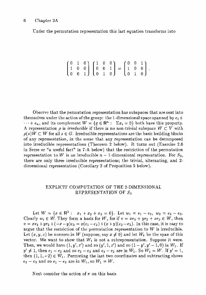
Under the permutation representation this last equation transforms into
Observe that the permutation representation has subspaces that are sent intothemselves under the action of the group: the I-dimensional space spanned by el +· . · + en, and its complement W = {f E Rn: ~Xi = O} both have this property.A representation p is irreducible if there is no non-trivial subspace W C V withp(s)W C W for all s E G. Irreducible representations are the basic building blocksof any representation, in the sense that any representation can be decomposedinto irreducible representations (Theorem 2 below). It turns out (Exercise 2.6in Serre or "a useful fact" in 7-A below) that the restriction of the permutationrepresentation to W is an irreducible n - I-dimensional representation. For 83 ,
there are only three irreducible representations; the trivial, alternating, and 2dimensional representation (Corollary 2 of Proposition 5 below).
EXPLICIT COMPUTATION OF THE 2-DIMENSIONALREPRESENTATION OF 53
Let W = {x E R3: Xl + X2 + X3 = O}. Let WI = el - e2, W2 = e2 - e3.Clearly Wi E W. They form a basis for W, for if v = xel + ye2 + ze3 E W, thenv = xel +ye2 +( -x-y)e3 = x(el-e2)+(x+y)(e2 -e3). In this case, it is easy toargue that the restriction of the permutation representation to W is irreducible.Let (x, y, z) be nonzero in W (suppose, say x =1= 0) and let W I be the span of thisvector. We want to show that WI is not a subrepresentation. Suppose it were.Then, we would have (1, y', z') and so (y', 1, z') and so (1 - y', y~ - 1, 0) in Wl. Ify' f:. 1, then el - e2 and so e2 - e3 and el - e2 are in Wl. So W l = W. If y' = 1,then (1, 1, -2) E Wl. Permuting the last two coordinates and subtracting showse2 - e3 and so el - e2 are in Wl , so Wl = W.
Next consider the action of 1r on this basis

Basics of Representations and Characters 7
1r p(1r )Wt p( 1r )W2 p(1r)
id Wt W2 (~ ~)
(1 2) -Wt Wt + W2 ( ~1 ~ )(2 3) Wl + W2 -W2 (i ~1)
(1 3) -W2 -Wl ( ~1 ~1 )
(1 2 3) -(Wl + W2) (~ -1)W2-1
(1 3 2) -(Wt + W2) ( -1 ~ )Wl -1
CONVOLUTIONS AND FOURIER TRANSFORMS
Throughout we will use the notion of convolution and the Fourier transform.Suppose P and Q are probabilities on a finite group G. Thus pes) 2:: 0, L;sP(s) =1. By the convolution P *Q we mean the probability P *Q( s) == 'EtP(st-1 )Q( t) :"first pick t from Q, then independently pick u from P and form the product ut."Note that in general P * Q =1= Q * P. Let the order of C be denoted ICI. Theuniform distribution on Gis U(s) == l/IGI for all s E G. Observe that U *U == Ubut this does not characterize U-the uniform distribution on any subgroup satisfiesthis as well. However, U * P == U for any P and this characterizes U.
Let P be a probability on G. The Fourier transform of P at the representation p is the matrix
pep) == 'EsP(s)p(s).
The same definitions works for any function P. In Proposition 11, we will showthat as p ranges over irreducible representations, the matrices Pep) determine P.
EXERCISE 1. Let p be any representation. Show p7Q(p) == F(p)Q(p).
EXERCISE 2. Consider the following probability (random transpositions) on S3
P(id) == p, P(12) == P(13) == P(23) = (1 - p)/3.
Compute T(p) for the three irreducible representations of S3. (You'll learn something.)
B. THE BASIC THEOREMS.
This section follows Serre quite closely. In particular, the theorems are numbered to match Serre.

8 Chapter 2B
Tlleorem 1. Let p: G ~ GL(V) be a linear representation of G in V andlet W be a subspace of V stable under G. Then there is a complement WO (soV = W + Wo, W n WO = 0) stable under G.
Proof. Let <, >1 be a scalar product on V. Define a new inner product by< u,V >= ~s < p(s)u, p(s)v >1. Then <,> is invariant: < p(s)u, p(s)v> = <u, v > . The orthogonal complement of W in V serves as Wo. 0
Remark 1. We will say that the representation V splits into the direct sum of Wand WO and write V = W EB Wo. The importance of this decomposition cannotbe overemphasized. It means we can study the action of G on V by separatelystudying the action of G on Wand Wo.
Remark 2. We have already seen a simple example: the decomposition of thepermutation representation of Sn. Here is a second example. Let Sn act on R2
by p(1r)(x, y) = sgn(1r)(x, y). The subspace W = {(x, y): x = y} is invariant.Its complement, under the usual inner product, is WO = {(x, y): x = -y} isalso invariant. Here, the complement is not unique. For example, Woo == {(x, y) :2x = -y} is also an invariant complement.
Remark 3. The proof of Theorem 1 uses the "averaging trick;" it is the standardway to make a function of several variables invariant. The second most widelyused approach, defining < u,v >2= maxg < p(g)u, p(g)v >1, doesn't work heresince <, >2 is not still an inner product.
Remark 4. The invariance of the scalar product <, > means that if ei is chosenas an orthonormal basis with respect to <, >, then < p(s)ei, p(s)ej > = bij .It follows that the matrices p(s) are unitary. Thus, if ever we need to, ,ve mayassume our representations are unitary.
Remark 5. Theorem 1 is true for compact groups. It can fail for noncompactgroups. For example, take G = IR under addition. Take" V as the set of linearpolynomials ax + b. Define p(t)f(x) = f(x + t). The constants form a non-trivialsubspace with no invariant complement. Theorem 1 can also fail over a finitefield.
Return to the setting of Theorem 1 by induction we get:
Theorem 2. Every representation is a direct sum of irreducible representations.
There are two ways of taking two representations (p, V) and (TJ, W) of thesame group and making a new representation. The direct sum constructs thevector space V EB W consisting of all pairs (v, w), v E V, w E W. The direct sumrepresentation p EB 1](s)(v, w) = (p( s )v, 1](s)w). This has dimension d p + dTJ andclearly contains invariant subspaces equivalent to V and W.
The tensor product constructs a new vector space V ® W of dimension dpdTJwhich can be defined as the set of formal linear combinations v ® w subject tothe rules (avl + bV2) ® w = a(VI ® w) + b(v2 ® w) (and symmetrically). If VI,..• , Va and W1, ••• , Wb are a basis for V and W, then Vi ® Wj is a basis for
Basics of Representations and Characters 9
v 0 W. Alternatively, V 0 W can be regarded as the set of a by b matrices werev 0 W has ij entry AifLj if v = :EAivi, W = :EJ.LjWj. The representation operates asP ® 7](s)(v ® w) = p(s)v ® 7](s)w.
The explicit decomposition of tensor products into direct sums is a boomingbusiness. New irreducible representations can be constructed from known onesby tensoring and decomposing.
The notion of the character of a representation is extraordinarily useful. If Pis a representation, define Xp( s) = Tr p(s). This doesn't depend on the basischosen for V because the trace is basis free.
PROPOSITION 1. If X is the character of a representation P of degree d then
(1) X(id) = d; (2) X(S-I) = X(s)*; (3) X(tst- I) = X(s).
Proof. (1) p(id) = id. (2) First p(sa) = I for a large enough. It follows that theeigenvalues Ai of p(s) are roots of unity. Then, with * complex conjugation,
X(s)* = Tr p(s)* = ~Ai = ~l/Ai == Tr p(s)-I == Tr pes-I) = X(s-I).
(3) Tr(AB) = Tr(BA). o
PROPOSITION 2. Let PI : G --* GL(VI ) and P2 : G --* GL(V2) be representationswith characters Xl and X2· Then (1) the character of PI EB P2 is Xl + X2 and (2)the character of PI 0 P2 is Xl · X2·
Proof. (1) Choose a basis so the matrix of PI EB P2 is given as (ti1 p~). (2) Thematrix of the linear map PI (s) 0 P2( s) is the tensor product of the matrices PI (s)and P2(S). This has diagonal entries p~lil(S)p~2j2(S). 0
Consider two representations P based on V and T based on W. They are calledequivalent if there is a 1-1 linear map f from V onto W such that T s 0 f == fops.For example, consider the following two representations of the symmetric group:p, the I-dimensional trivial representation (so V = IR and p(7r)x = x) and T, therestriction of the n-dimensional permutation representation to the subspace Wspanned by the vector el +···+en. Here r( 1r )x(et +···+ en) = x(et +···+en).The isomorphism can be taken as I( x) = x(el + · · .+ en).
The following "lemma" is one of the most used elementary tools.
SCHUR'S LEMMA
Let pI: G --* GL(VI ) and p2 : G ~ GL(V2 ) be two irreducible representations of G, and let f be a linear map of VI into V2 such that
p~ 0 f = f 0 p~ for all s E G.
Then(1) If pI and p2 are not equivalent, we have f = o.
10 Chapter 2B
(2) If VI == V2 and pI == p2, f is a constant times the identity.
Proof. Observe that the kernel and image of f are both invariant subspaces. Forthe kernel, if f(v) == 0, then fp~(v) == p;j(v) == 0, so p~(v) is in the kernel. Forthe image, if w = f( v), then p;(w) = f p~(v) is in the image too. By irreducibility,both kernel and image are trivial or the whole space. To prove (1) suppose f f:. o.Then Ker = 0, image == V2 and / is an isomorphism. To prove (2) suppose / =I 0(if / = 0 the result is true). Then / has a non-zero eigenvalue A. The mapfl == / - AI satisfies p;/1 == /1 p~ and has a non-trivial kernel, so /1 == O. 0
EXERCISE 3. Recall that the uniform distribution is defined by U(s) = l/IGI,where IGI is the order of the group G. Then at the trivial representation fJ(p) == 1and at any non-trivial irreducible representation fJ(p) = o.
There are a number of useful ways of rewriting Schur's lemma. Let IGI bethe order of G.
COROLLARY 1. Let h be any linear map of VI into V2 • Let
ho 1 ~( 2)-lh 1== fGT~ Pt Pt·
Then(1) If pI and p2 are not equivalent, hO == O.(2) If VI == V2 and pI == p2, then h° is a constant times the identity, the constantbeing Trh/d p •
P f F 2 hO 1 - 1 ~ 2 h 1 - 1 ~( 2 )-1 h 1 - hO Ifroo. or any s, Ps-l Ps - TGT~Ps-lt-l Pts - TGT~ Pts Pts - ·pI and p2 are not isomorphic then hO = 0 by part (1) of Schur's lemma. IfVI == v2 , PI == P2 == p, then by part (2), hO == cl. Take the trace of both sidesand solve for c. 0
The object of the next rewriting of Schur's lemma is to show that the matrixentries of the irreducible representations form an orthogonal basis for all functionson the group G. For compact groups, this sometimes is called the Peter-Weyltheorem.
Suppose pI and p2 are given in matrix form
The linear maps hand hO are defined by matrices Xi2 i1
and X?2 i l. We have
In case (1), hO == 0 for all choices of h. This can only happen if the coefficients ofx i2il are all zero. This gives
Basics of Representations and Characters 11
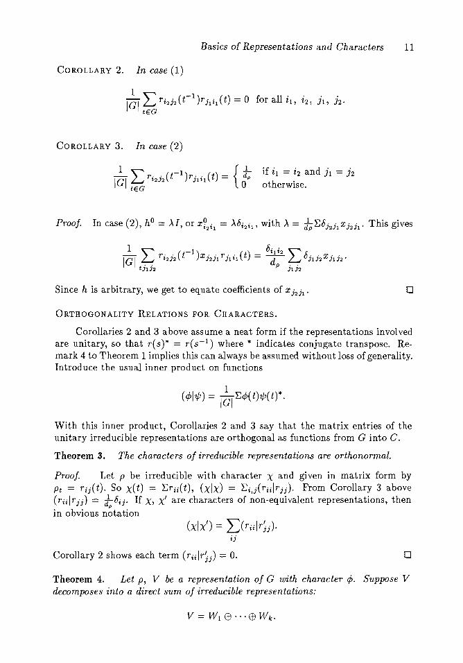
COROLLARY 2. In case (1)
COROLLARY 3. In case (2)
if i 1 == i 2 and j1 == j2
otherwise.
Since h is arbitrary, we get to equate coefficients of x j2jl • o
ORTHOGONALITY RELATIONS FOR CHARACTERS.
Corollaries 2 and 3 above assume a neat form if the representations involvedare unitary, so that r(s)* == r(S-l) where * indicates conjugate transpose. Remark 4 to Theorem 1 implies this can always be assumed without loss of generality.Introduce the usual inner product on functions
(4)I,,p) = I~I I;4>( t)"p( t) *.
With this inner product, Corollaries 2 and 3 say that the matrix entries of theunitary irreducible representations are orthogonal as functions from G into C.
Theorem 3. The characters of irreducible representations are orthonormal.
Proof. Let P be irreducible with character X and given in matrix form byPt == rij(t). So X(t) == Erii(t), (xix) == Ei,j(riifrjj). From Corollary 3 above(riilrjj) == d1 Dij. If X, X' are characters of non-equivalent representations, then
p
in obvious notation
(xIx') = I)riilrjj)'ij
Corollary 2 shows each term (riilrjj) == o. o
Theorem 4. Let p, V be a representation of G with character cP. Suppose Vdecomposes into a direct sum of irreducible representations:
12 Chapter 2C
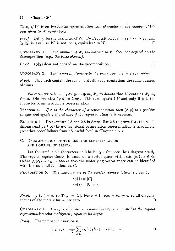
Then, if W is an irreducible representation with character X, the number of W i
equivalent to W equals (1)1 X).
Proof. Let Xi be the character of W i • By Proposition 2,1> = Xl + · · ·+ Xk, and(xilx) is 0 or 1 as Wi is not, or is, equivalent to W. 0
COROLLARY 1. The number of Wi isomorphic to W does not depend on thedecomposition (e.g., the basis chosen).
Proof. (1)lx) does not depend on the decomposition. o
COROLLARY 2. Two representations with the same character are equivalent.
Proof. They each contain the same irreducible representations the same numberof times. 0
We often write V = ml W I EB · · · Et) m n W n to denote that V contains W i mi
times. Observe that (1)11>) = ~mr. This sum equals 1 if and only if 1> is thecharacter of an irreducible representation.
Theorem 5. If 1> is the character of a representation then (1)11>) is a positiveinteger and equals 1 if and only if the representation is irreducible.
EXERCISE 4. Do exercises 2.5 and 2.6 in Serre. Use 2.6 to prove that the n - 1dimensional part of the n-dimensional permutation representation is irreducible.(Another proof follows from "A useful fact" in Chapter 7-A.)
c. DECOMPOSITION OF THE REGULAR REPRESENTATION
AND FOURIER INVERSION.
Let the irreducible characters be labelled Xi. Suppose their degrees are dieThe regular representation is based on a vector space with basis {e s}, sEC.Define ps(et) = est. Observe that the underlying vector space can be identifiedwith the set of all functions on C.
PROPOSITION 5. The character rG of the regular representation is given by
TG(l) = ICITG(S) = 0, S =11.
Proof. PI(es) = es so Tr PI = ICI. For s f: 1, pset = est f; et so all diagonalentries of the matrix for Ps are zero. 0
COROLLARY 1. Every irreducible representation W i is contained in the regularrepresentation with multiplicity equal to its degree.
Proof. The number in question is
(rGIXi) = I~I L rG(s)xi(s) = Xi(l) = di .sEG
o

Basics of Representations and Characters 13
Remark. Thus, in particular, there are only finitely many irreducible representations.
COROLLARY 2.(a) The degrees di satisfy ~d; == fGf.(b) If s E G is different from 1, ~diXi(S) == o.Proof. By Corollary 1, Ta(S) == ~diXi(S). For (a) take s == 1, for (b) take anyother s. 0
In light of remark 4 to Theorem 1, we may always choose a basis so thematrices Tij( s) are unitary.
COROLLARY 3. The matrix entries of the unitary irreducible representationsform an orthogonal basis for the set of all functions on G.
Proof. We already know the matrix entries are all orthogonal as functions.There are ~d; == IGI of them, and this is the dimension of the vector space of allfunctions. 0
In practice it is useful to have an explicit formula expressing a function inthis basis. The following two results will be in constant use.
PROPOSITION.
(a) Fourier Inversion Theorem. Let f be a function on G, then
(b) Plancherel Formula. Let f and h be functions on G, then
-1 1 ,.,.'L.f(S )h(s) = ICI'L.di Tr(f(pi)h(pi)).
Proof. Part (a). Both sides are linear in f so it is sufficient to check the formulafor f(s) == bst . Then !(Pi) == pi(t), and the right side equals
1 -1jGf'L.diXi(S t).
The result follows from Corollary 2.
Part (b). Both sides are linear in f; taking f(s) == bst, we must show
This was proved in part (a). o
14 Chapter 2D
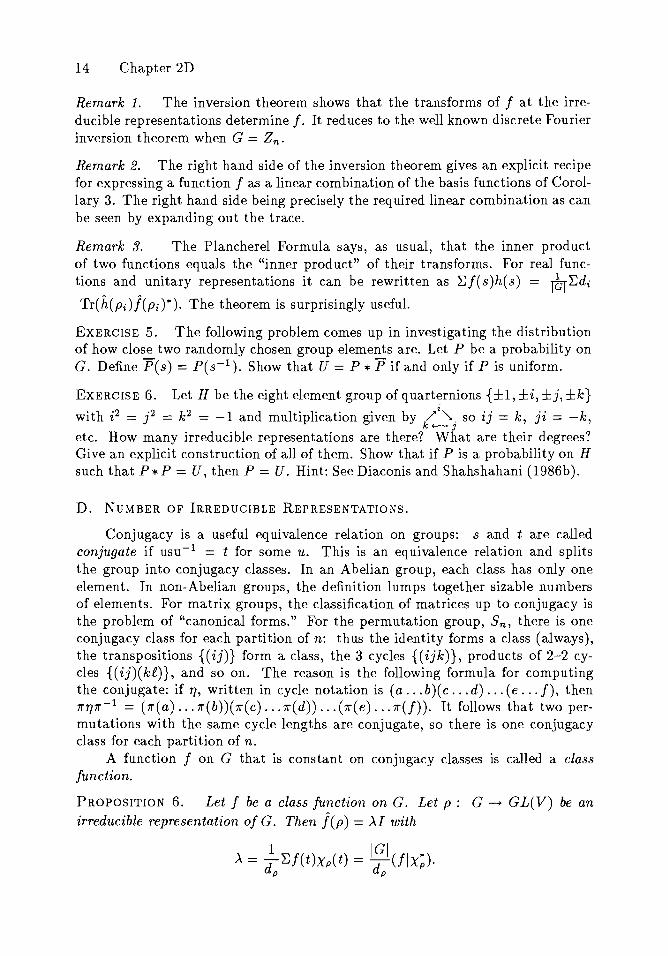
Remark 1. The inversion theorem shows that the transforms of f at the irreducible representations determine f. It reduces to the well known discrete Fourierinversion theorem when G == Zn.
Remark 2. The right hand side of the inversion theorem gives an explicit recipefor expressing a function f as a linear combination of the basis functions of Corollary 3. The right hand side being precisely the required linear combination as canbe seen by expanding out the trace.
Remark 3. The Plancherel Formula says, as usual, that the inner productof two functions equals the "inner product" of their transforms. For real functions and unitary representations it can be rewritten as "£f( s)h(s) == Ibl"£di
Tr(h(pi)j(pi)*). The theorem is surprisingly useful.
EXERCISE 5. The following problem comes up in investigating the distributionof how close two randomly chosen group elements are. Let P be a probability onG. Define pes) == P(s-l). Show that U == P * P if and only if P is uniform.
EXERCISE 6. Let H be the eight element group of quarternions {±1, ±i, ±j, ±k}i
with i2 == j2 = k2 == -1 and multiplication given by /~. so ij == k, ji = -k,k+--J
etc. How many irreducible representations are there? What are their degrees?Give an explicit construction of all of them. Show that if P is a probability on Hsuch that P *P == U, then P == U. Hint: See Diaconis and Shahshahani (1986b).
D. NUMBER OF IRREDUCIBLE REPRESENTATIONS.
Conjugacy is a useful equivalence relation on groups: sand t are calledconjugate if usu-1 = t for some u. This is an equivalence relation and splitsthe group into conjugacy classes. In an Abelian group, each class has only oneelement. In non-Abelian groups, the definition lumps together sizable numbersof elements. For matrix groups, the classification of matrices up to conjugacy isthe problem of "canonical forms." For the permutation group, Sn, there is oneconjugacy class for each partition of n: thus the identity forms a class (always),the transpositions {(ij)} form a class, the 3 cycles {(ijk)}, products of 2-2 cycles {(ij)(k£)}, and so on. The reason is the following formula for computingthe conjugate: if'TJ, written in cycle notation is (a ... b)(c ... d) ... (e ... f), then1r'TJ1r-1 == (1r(a) ... 1r(b))(1r(c) ... 1r(d)) .. . (1r(e) .. .1r(f)). It follows that two permutations with the same cycle lengths are conjugate, so there is one conjugacyclass for each partition of n.
A function f on G that is constant on conjugacy classes is called a classfunction.
PROPOSITION 6. Let f be a class function on G. Let p: G ~ GL(V) be anirreducible representation of G. Then j(p) == AI with
Basics of Representations and Characters 15
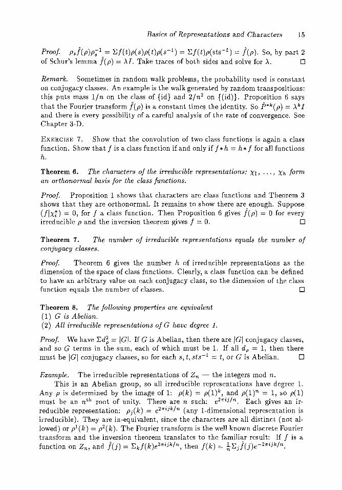
Proof. Psl(p)p;l = ~f( t)p( 8 )p(t)p(8-1 ) = ~f( t)p(sts-1 ) = l(p). So, by part 2of Schur's lemma l(p) = AI. Take traces of both sides and solve for A. 0
Remark. Sometimes in random walk problems, the probability used is constanton conjugacy classes. An example is the walk generated by random transpositions:this puts mass I/n on the class of {id} and 2/n2 on {(id)}. Proposition 6 saysthat the Fourier transform j(p) is a constant times the identity. So P*k(p) = AkIand there is every possibility of a careful analysis of the rate of convergence. SeeChapter 3-D.
EXERCISE 7. Show that the convolution of two class functions is again a classfunction. Show that f is a class function if and only if f *h == h*f for all functionsh.
Theorem 6. The characters of the irreducible representations: Xl, ... , Xh forman orthonormal basis for the class functions.
Proof. Proposition 1 shows that characters are class functions and Theorem 3shows that they are orthonormal. It remains to show there are enough. Suppose(flxt) == 0, for f a class function. Then Proposition 6 gives l(p) == 0 for everyirreducible p and the inversion theorem gives f == O. 0
Tlleorem 7. The number of irreducible representations equals the number ofconjugacy classes.
Proof Theorem 6 gives the number h of irreducible representations as thedimension of the space of class functions. Clearly, a class function can be definedto have an arbitrary value on each conjugacy class, so the dimension of the classfunction equals the number of classes. 0
Theorem 8. The following properties are equivalent(1) G is Abelian.(2) All irreducible representations of G have degree 1.
Proof We have ~d~ == IGI. If G is Abelian, then there are IGI conjugacy classes,and so G terms in the sum, each of which must be 1. If all dp == 1, then theremust be IGI conjugacy classes, so for each s, t, sts- 1 == t, or G is Abelian. 0
Example. The irreducible representations of Zn - the integers mod n.This is an Abelian group, so all irreducible representations have degree 1.
Any p is determined by the image of 1: p(k) == p(l)k, and p(l)n == 1, so p(1)must be an nth root of unity. There are n such: e21rij/n. Each gives an irreducible representation: pj(k) == e21rijk/n (any I-dimensional representation isirreducible). They are in-equivalent, since the characters are all distinct (not allowed) or pI (k) == p2 (k). The Fourier transform is the well known discrete Fouriertransform and the inversion theorem translates to the familiar result: If f is afunction on Zn, and l(j) == ~kf(k)e21rijk/n, then f(k) = ~~jj(j)e-21rijk/n.
16 Chapter 2E
E. PRODUCT OF GROUPS.
If G I and G2 are groups, their product is the set of pairs (91,92) with multiplication defined coordinate-wise. The following considerations show that therepresentation theory of the product is determined by the representation theoryof each factor.
Let pI: G1 ~ GL(V1 ) and p2: G2 ~ GL(V2) be representations. DefinepI 0 p2: GI X G2~ GL(VI 0 V2) by
pI ® Pts,t)(VI ® V2) = p~(VI) ® p~(V2).
This is a representation with character Xl (s) · X2 (t).
Theorem 9.(1) If pI and p2 are irreducible, then pI ® p2 is irreducible.(2) Each irreducible representation of G I X G2 is equivalent to a representationpI 0 p2 1vhere pi is an irreducible representation of G i •
Proof.(1) (xllxl) = (x2Ix2) = 1, but the norm of the character of PI ® P2 is
IGIIIG21~Xl(S)X2(t)XI(S)*X2(t)* = (xllxl)·(X2Ix2) = 1. So Theorem 5 givesirreducibility.
(2) The characters of the product representation are of the form Xl · X2. It isenough to show these form a basis for the class functions on G I X G2 • Sincethey are all characters of irreducible representations, they are orthonorlnal,so it must be proved that they are it all of the possible characters. If f( s, t)is a class function orthogonal to all XI(S)X2(t), then
Then for each t, ~f(s, t)XI(S)* = 0, so f(s, t) = 0 for each t. o
EXERCISE 8. Compute all the irreducible representations of Z~, explicitly.We now leave Serre to get to applications, omitting the very important topic
of induced representations. The most relevant material is Section 3.3, Chapter 7,and Sections 8.1,8.2. A bit of it is developed here in Chapter 3-F.
Chapter 3. Random Walks on Groups
A. EXAMPLES
A fair number of real world problems lead to random walks on groups. Thissection contains examples. It is followed by more explicit mathematical formulations and computations.
1. RANDOM WALK ON THE CIRCLE AND RANDOM NUMBER GENERATION
Think of Zp (the integers mod p) as p points wrapped around a discretecircle. The simplest random walk is a particle that moves left or right, each withprobability t. We can ask: how many steps does it take the particle to reach agiven site? How many steps does it take the particle to hit every site? After howmany steps is the distribution of the particle close to random? In Section C, weshow that the answer to all of these questions is about p2.
A class of related problems arises in computer generation of pseudo randomnumbers based on the recurrence X k+l = aXk + b(mod p) where p is a fixednumber (often 232 or the prime 231 - 1) and a and b are chosen so that thesequence X o = 0, Xl, X 2 , ••• , has properties resembling a random sequence. Anextensive discussion of these matters is in Knuth (1981).
Of course, the sequence X k is deterministic and exhibits many regular aspects. To increase randomness several different generators may be combined or"shuffled." One way of shuffling is based on the recurrence X k+1 = akXk + bk(mod p) where (ak' bk) might be the output of another generator or might be theresult of a "true random" source as produced by electrical or radioactive noise.We will study how a small amount of randomness for a and b spreads out torandomness for the sequence X k •
If ak == 1 and bk takes values ±1 with probability t, we have a simple randomwalk. If ak =1= 1 is fixed but nonrandom, the resulting process can be analyzed byusing Fourier analysis on Zp. In Section C we show that if ak == 2, then aboutlog p loglog p steps are enough to force the distribution of Xk to be close touniform (with bk taking values 0, ±1 uniformly). This is a great deal faster thanthe p2 steps required when ak == 1. If ak == 3, then log p steps are enough.
What if ak is random? Then it is natural to study the problem as a randomwalk on Ap - the affine group mod p. This is the set of pairs (a, b) with a, b EZp, a ~ 0, gcd(a, p) = 1. Multiplication is defined by
(a,b)(c,d) = (ac, ad +b).
Some results are in Example 4 of Section C, but many simple variants are unsolved.
17
18 Chapter 3A
A different group arises when considering the second order recurrence Xk+l =akXk+bkXk-l (mod p) with a and b random. It is natural to define Yk = (x:~),
then
This leads to considering a product of random matrices, and so to a random walkon GL2(Zp). See Diaconis and Shahshahani (1986a) for some results.
2. CARD SHUFFLING
How many times must a deck of cards be shuffled until it is close to random?Historically, this was a fairly early application of probability. Markov treated itas one of his basic examples of a Markov chain (for years, the only other examplehe had was the vowel/consonant patterns in Eugene Onegin). Poincare devotedan appendix of his 1912 book on probability to the problem, developing methodssimilar to those in Section C. The books by Doob (1935) and Feller (1968) eachdiscuss the problem and treat it by Markov chain techniques.
All of these authors show that any reasonable method of shuffling will eventually result in a random deck. The methods developed here allow explicit rates thatdepend on the deck size. As will be explained, these are much more accurate thanthe rates obtained by using bounds derived from the second largest eigenvalue ofthe associated transition matrix.
Some examples of specific shuffles that will be treated below:a) Random transpositions. Imagine n cards in a row on a table. The cards
start in order, card 1 at the left, card 2 next to it, ..., and card n at the right ofthe row. Pairs of cards are randomly transposed as follows: the left had touchesa random card, and the right hand touches a random card (so left = right withprobability ~). The two cards touched are interchanged. A mathematical modelfor this process is the following probability distribution on the symmetric group:
T(id) = !.n
T(T) = ~ for T any transpositionn
T(1r) = 0 otherwise.
Repeatedly transposing cards is equivalent to repeatedly convolving T with itself.It will be shown that the deck is well mixed after tn log n + en shuffles.
Some variants will also be discussed: repeatedly transposing a random cardwith the top card (la Librairie de la Marguerite), or repeatedly interchanging acard with one of its neighbors.
b) Borel's shuffle. In a book on the mathematics of Bridge, Borel and Cheron(1955) discuss the mathematics of shuffling cards at length. They suggest severalopen problems; including the following shuffle: The top card of a deck is removedand inserted at a random position, then the bottom card is removed and insertedat a random position. This is repeated k times. We will analyze such procedures
Random Walks on Groups 19
in Chapter 4, showing that k = n log n + en "moves" are enough. The sametechniques give similar rates for the shuffle that repeatedly puts a random cardon top, or the shuffle that repeatedly removes a card at random and replaces itat random.
c) Riffle shuffles. This is the usual way that card players shuffle cards,cutting off about half the pack and riffling the two packets together. In Chapter4 we will analyze a model for such shuffles due to Gilbert, Shannon, and Reeds.We will also analyze records of real riffle shuffles. The analysis suggests that 7shuffles are required for 52 cards.
d) Overhand shuffles. This is another popular way of shuffling cards. Thefollowing mathematical model seems reasonable: the deck starts face down in thehand. Imagine random zeros and ones between every pair of cards with a zerounder the bottom card of the deck. Lift off all the cards up to the first zero andplace them on the table. Lift off all the cards up to the second zero and place thispacket on top of the first removed packet. Continue until no cards remain. Thisis a single shuffle. It is to be repeated k times. Robin Pemantle (1988) has shownthat about 2500 shuffles are required for 52 cards.
3. RANDOM WALK ON THE d-CUBE ztRegard zt as the vertices of a cube in d dimensions. The usual random walk
starts at a point and moves to one of the d neighbors with probability ~. This isrepeated k times. This is a nice problem on its own. It has a surprising connectionwith a classical problem in statistical mechanics: in the Ehrenfest's urn model, dballs are distributed in two urns. A ball is chosen at random and moved to theother urn. This is repeated k times and the problem is to describe the limitingdistribution of the process. For a fascinating description of the classical approachsee M. Kac (1947). Kac derives the eigenvalues and eigenvectors of the associatedtransition matrix by a tour de force. The following approach due to Siegert (1949)suggests much further research:
Let the state of the system be described by a binary vector of length d, witha 1 in the ith place denoting that ball i is in the right hand urn. The transitionmechanism translates precisely to a random walk on the d cube! Indeed, the statechanges by picking a coordinate and changing to its opposite mod 2. This changesthe problem into analyzing the behavior of a random walk on an Abelian group.As we will see, this is straightforward; Fourier analysis gives all the eigenvaluesand eigenvectors of the associated Markov chain.
Originally the state of the system in the Ehrenfest's urn was the numberof balls in the right hand urn. The problem was "lifted" to a random walk ona group. That is, there was a group G (here Z1) and a probability P on G(here move to the nearest neighbor) and a function L: G --* state space (here thenumber of ones) such that the image law under L of the random walk was thegiven Markov chain. There has been some study of the problem of when the imageof a Markov chain is Markov. HelIer (1965) contains much of interest here. MarkKac was fascinated with this approach and asked: When can a Markov chainbe lifted to a random walk on a group? Diaconis and Shahshahani (1987b) giveresults for "Gelfand Pairs." The following exercise comes out of discussions with
20 Chapter 3A
Mehrdad Shahshahani.
EXERCISE 1. Let P be a probability on the symmetric group Sn. Think of therandom walk generated by P as the result of repeatedly mixing a deck of n cards.For a permutation 1r, let L(1r) = 1r(1). The values of L are the result of followingonly the position of card 1. Show that the random walk induces a Markov chainfor L. Show that this chain has a doubly stochastic transition matrix. Conversely,show that for any doubly stochastic matrix, there is a probability P on Sn whichyields the given matrix for L.
Remark. It would be of real interest to get analogs of this result more generally.For example: find conditions on a Markov chain to lift to a random walk on anAbelian group. Find conditions on a Markov chain to lift to a random walk witha probability P that is constant on conjugacy classes. When can a Markov chainon the ordinary sphere be lifted to a random walk on the orthogonal group 0 3?
Returning to the cube, David Aldous (1983b) has applied results from randomwalk on the d cube to solve problems in the theory of algorithms. Eric Lander(1986) gives a very clear class of problems in DNA gene mapping which reallyinvolves this process. Diaconis and Smith (1986) develop much of the fluctuationtheory of coin-tossing for the cube. There is a lot going on, even in this simpleexample.
4. INFINITE GROUPS
For the most part, these notes treat problems involving finite groups. However, the techniques and questions are of interest in solving applied problemsinvolving groups like the orthogonal group and p-adic matrix groups. Here is abrief description.
1. The "Grand Tour" and a walk on On. Statisticians often inspect highdimensional data by looking at low-dimensional projections. To give a specificexample, let Xl, ••• , Xsoo f R20 represent data on the Fortune 500 companies.Here Xl, the data for company 1, might have coordinates XII == total value,Xl2 == number of women employed, etc.. For / f R20 , the projection in direction /would be a plot (say a histogram) of the 500 numbers I· Xl, ••• ,/. Xsoo. Similarlythe data would be projected onto various two-dimensional spaces and viewed asa scatterplot. Such inspection is often done interactively at a computer's displayscreen, and various algorithms exist for changing the projection every few secondsso that a scientist interested in the data can hunt for structured views.
Such algorithms are discussed by D. Asimov (1983). In one such, the directionI changes by a small, random rotation. Thus, one of a finite collection fi of 20 X 20orthogonal matrices would be chosen at random, and the old view is rotated byf i . This leads to obvious questions such as, how long do we have to wait untilthe views we have seen come within a prescribed distance (say 5 degrees) of anyother view. A good deal of progress on this problem has been made by PeterMatthews in his Stanford Ph.D. thesis. Matthews (1988a) uses Fourier analysison the orthogonal group and diffusion approximations to get useful numerical andtheoretical results.
(1)
Random Wall,s on Groups 21
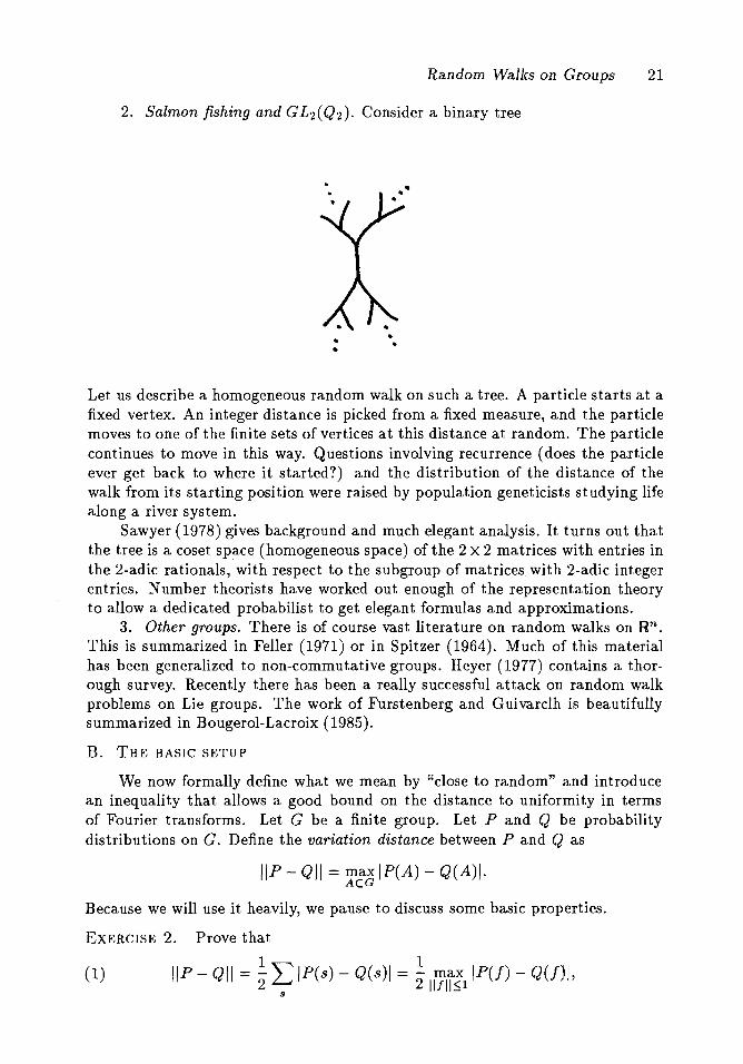
2. Salmon fishing and GL2(Q2). Consider a binary tree
Let us describe a homogeneous random walk on such a tree. A particle starts at afixed vertex. An integer distance is picked from a fixed measure, and the particlemoves to one of the finite sets of vertices at this distance at random. The particlecontinues to move in this way. Questions involving recurrence (does the particleever get back to where it started?) and the distribution of the distance of thewalk from its starting position were raised by population geneticists studying lifealong a river system.
Sawyer (1978) gives background and much elegant analysis. It turns out thatthe tree is a coset sp~ce (homogeneous space) of the 2 X 2 matrices with entries inthe 2-adic rationals, with respect to the subgroup of matrices. with 2-adic integerentries. Number theorists have worked out enough of the representation theoryto allow a dedicated probabilist to get elegant formulas and approximations.
3. Other groups. There is of course vast literature on random walks on Rn.This is summarized in Feller (1971) or in Spitzer (1964). Much of this materialhas been generalized to non-commutative groups. Heyer (1977) contains a thorough survey. Recently there has been a really successful attack on random walkproblems on Lie groups. The work of Furstenberg and Guivarclh is beautifullysummarized in Bougerol-Lacroix (1985).
B. THE BASIC SETUP
We now formally define what we mean by "close to random" and introducean inequality that allows a good bound on the distance to uniformity in termsof Fourier transforms. Let G be a finiie group. Let P and Q be probabilitydistributions on G. Define the variation distance between P and Q as
liP - QII = Pta IP(A) - Q(A)/.
Because we will use it heavily, we pause to discuss some basic properties.
EXERCISE 2. Prove that
liP - QII = ~L IP(s) - Q(s)1 = ~ Imi~lIPU) - QU)I,s
22 Chapter 3B
where, in the last expression, f is a function from G to IR with If( s)1 :::; 1, andP(f) = 'EsP(s)f(s) is the expected value of f under P. Also, prove the validityof the following interpretation of variation distance suggested by Paul Switzer:Given a single observation, coming from P or Q with probability t, you are toguess which. Your chance of being correct is t + t 11 P - Q11·
EXERCISE 3. Show that if U is uniform, and h: G ---T G is 1 - 1, then
liP - UII = IIPh- l - UII where Ph-leA) = P(h-l(A)).
EXERCISE 4. Let G = Sn. Part (a): let P be defined by "card 1 is on top,all the rest are random." Thus, P(1r) = 0 if 1r(1) ~ 1 and P(1r) = 1/(n - 1)!otherwise. What is IIP-UII? Part (b): suppose P is defined by "card 1 is randomlydistributed in a fixed set A of positions, all the other cards are random?" Whatis liP - UII?
Further properties of the variation distance are given in the following remarksand in lemma 4 of Chapter 3, lemma 4 of Chapter 4 and lemma 5 of Chapter 4.
Remark 1. The variation distance can be defined for any measurable group. Itmakes the measures on G into a Banach space. For G compact, the measuresare the dual of the bounded continuous functions and 1I 11 is the dual norm. Forcontinuous groups, the variation distance is often not suitable, since the distancebetween a discrete and continuous probability is 1. In this case, one picks anatural metric on G, and uses this to metrize the weak-star topology. Of course,for finite groups, all topologies are equivalent and the variation distance is chosenbecause of the natural interpretation given by (1): if two probabilities are closein variation distance, they give practically the same answer for any question.
Remark 2. Consider a random walk on Sn. In the language of shuffling cards, itmight be thought that the following notion would be a more suitable definition ofwhen cards are close to uniformly well shuffled: suppose the cards are turned faceup one at a time and we try to guess at the value of each card before it is shown.For the uniform distribution, as in Diaconis and Graham (1977), we expect to getH n = 1 + ~ + t + ··.+*right on average. If the deck is not well mixed, theincrease in the number of cards we can guess correctly seems like a useful measureof how far we are from uniform. Formally, one may define a guessing strategy foreach possible history. Its value on a given permutation 1r defines a function f( 1r)and (1) shows that, on average, /P(f)-Hn / < nIlP-UII no matter what guessingstrategy is used. This may serve as a guide for how small a distance liP - UII toaim for.
Remark 3. The variation distance is closely related to a variety of other metrics.For example, two other widely used measures of distance between probabilities
Random Wall{s on Groups 23
are
s
I(P, Q) =L pes) log[P(s)/Q(s)] - Kullback-Leibler separation.s
These satisfy
d; ~ 11 11 ~ VdH(1- dH/4) ~ .jJ;
V211 If ~ VI.It follows that when dH or I are small, the variation distance is small. Theconverse can be shown to hold under regularity conditions.
Metrics on probabilities are discussed by Dudley (1968), Zolatorev (1983)and Diaconis and Zabell (1982). Rachev (1986) is a recent survey.
THE BASIC PROBLEM.
We can now ask a sharp mathematical question: Let P be a probability onG. Given c > 0, how large should k be so that IIp*k - UII < e?
It is not hard to show that p*k tends to uniform if P is not concentrated ona subgroup or a coset of a subgroup. Here is a version of the theorem due to Koss(1959):
Theorem 1. Let G be a compact group. Let P be a probability on G such thatfor some no and c, 0 < c < 1, for all n > no,
(*)
Then, for all k,
p*n(A) > cU(A) for all open sets A.
Remarks. Condition * rules out periodicity. The conclusion shows that eventuallythe variation distance tends to zero exponentially fast. The result seems quantitative, but it's hard to use it to get bounds in concrete problems: as an example,consider simple random walk on Zn. How large must k be to have the distanceto uniform less than lo? To answer, we must determine a suitable no and c. Thisseems difficult. A short proof of the theorem is given here in Chapter 4.
There is a huge literature relating to this theorem. Heyer (1977) contains anextensive survey. Bhattacharya (1972) and Major and Shlossman (1979) containquantitative versions which are more directly useable. Csiszar (1962) gives aproof which indicates "why it is true": briefly, convolving increases entropy andthe maximum entropy distribution is the uniform. Bondesson (1983) discussesrepeated convolutions of different measures.
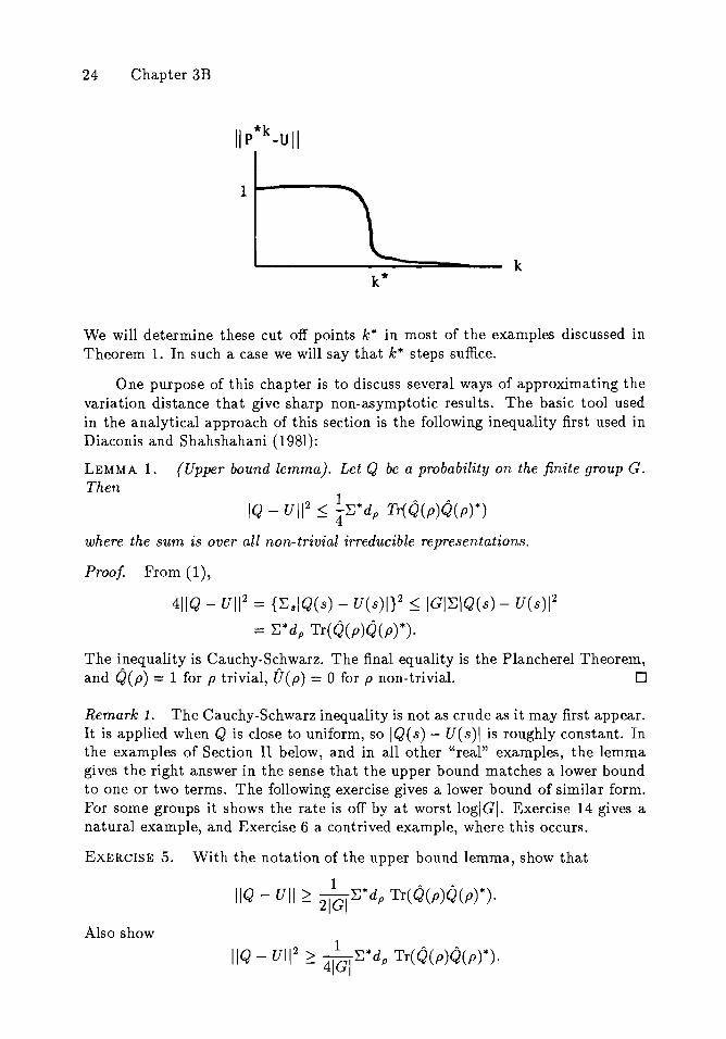
Remark. The following "cut off" phenomena occurs in most cases ,vhere thecomputations can be done: the variation distance, as a function of k, is essentially1 for a time and then rapidly becomes tiny and tends to zero exponentially fastpast the cut off. Thus a graph might appear
24 Chapter 3B
kk*
We will determine these cut off points k* in most of the examples discussed inTheorem 1. In such a case we will say that k* steps suffice.
One purpose of this chapter is to discuss several ways of approximating thevariation distance that give sharp non-asymptotic results. The basic tool usedin the analytical approach of this section is the following inequality first used inDiaconis and Shahshahani (1981):
LEMMA 1. (Upper bound lemma). Let Q be a probability on the finite group G.Then
IIQ - UI1 2 ~ l~*dp Tr(Q(p)Q(p)*)
where the sum is over all non-trivial irreducible representations.
Proof. From (1),
411Q - UI1 2 = {~sIQ(s) - U(s)I}2 ~ IGI~IQ(s) - U(s)1 2
= ~*dp Tr(Q(p)Q(p)*).
The inequality is Cauchy-Schwarz. The final equality is the Plancherel Theorem,and Q(p) = 1 for p trivial, U(p) = 0 for p non-trivial. 0
Remark 1. The Cauchy-Schwarz inequality is not as crude as it may first appear.It is applied when Q is close to uniform, so IQ(s) - U(s)1 is roughly constant. Inthe examples of Section 11 below, and in all other "real" examples, the lemmagives the right answer in the sense that the upper bound matches a lower boundto one or two terms. The following exercise gives a lower bound of similar form.For some groups it shows the rate is off by at worst loglGI. Exercise 14 gives anatural example, and Exercise 6 a contrived example, where this occurs.
EXERCISE 5. With the notation of the upper bound lemma, show that
1 A A
IIQ - UII ~ 21GI ~*dp Tr(Q(p)Q(p)*).
Also show
IIQ - uI1 2 ~ 41~1 ~*dp Tr(Q(p)Q(p)*).
Random Wall(s on Groups 25
EXERCISE 6. Let G be a finite group. Define a probability P on G by
P(id) = 1 - ~, P(s) = 2(1G; _ 1) for s # id, 0 ~ c ~ 2.
Show thatP*kCd) =~ IGI-1(1 _ ~ IGI )k
1 IGI + IGI 2 IGI - 1
*k lIe IGI kP (s) = jGj - jGj(1- 2" IGI- 1) ·
Using this, show that II p *k - UII = 1~t11 11 - ~ IJfi1l k• Show that
E*d Tr(P(p)kp) = (IGI- 1)(1 _ ~ IGI )2kp 21GI- 1 ·
Remark 2. Lower bounds can be found by choosing a set A C G and usingIQ(A) - U(A)I ~ IIQ - UII· Often A can be chosen so that it is possible tocalculate, or approximate, both Q(A) and U(A), and show that the distancebetween them is large. Several examples are given in the next section.
Remark 3. Total variation is used almost exclusively for the next two chapters.It is natural to inquire about the utility of the mathematically tractable L2 norm
2 1 2liP - Ulb = E(P(s) - IGI) ·
This has a fatal flaw: Suppose IGI is even, and consider P uniformly distributedover half the points and zero on the others. liP - UI'2 == -b is close to zero
vlGIfor IGllarge. Thus the interpretability of the L2 norm depends on the size of thegroup. This makes it difficult to compare rates as the size of the group increases.
The norm IGI!IIP - UI12 corrects for this. It seems somewhat artificial, andin light of the upper bound lemma and exercise 5, it is essentially the same as thevariation distance.
c. SOME EXPLICIT COMPUTATIONS
Example 1. Simple random walk on the circle. Consider Zp, the additive groupof integers mod p. Define P(l) == P( -1) == ~, P(j) == 0 otherwise. The following result shows that somewhat more than p2 steps are required to get close touniform.
Theorem 2. For n ~ p2, with p odd and greater than 7,
IIP*n - uti ~ e-on/ p2with a = 1("2 /2.
26 Chapter 3C
Conversely, for p ~ 7 and any n
Proof. The Fourier transform of P is
The upper bound lemma yields
1 p-l 1 (p-l)/2
\Ip*n - uW ::; 4L cos(27rjjp)2n = 2" L cos(7rjjp?n.j=l j=l
To bound this sum, use properties of cosine. One neat way to proceed was suggested by Hansmartin Zeuner: use the fact
This follows from h(x) == log(ex2 /2cos x), h'(x) == x - tan x ~ 0; so h(x) ~ h(O) =0, for x f [0, 1r /2].
This gives
(p-2)/2 00
IIP*n - UI1 2 ::; ~ L e-7[2j2 n / p2::; ~e-7[2n/p2L e-7[2(j2-1)n/p2
j=l j=l
00
< !.e-1r2n/p2~ e-31r2 jn/p2- 2 LJ
j=O
1 e-1r2n/p2
== 2' 1 - e-31r2n/p2 .
This works for any n and any odd p. If n 2:: p2, [2(1 - e-31r2
)] -1 < 1 and thus wehave proved more than we claimed for an upper bound.
Observe that the sum in the upper bound is dominated by the term withk = p;l. This suggests using the function cos(21rkj/p) alone to give a functionbounded by 1 which has expected value zero under the uniform distribution. Usingthe symmetry of P,
Now, (1) in section B above yields
Random Walks on Groups 27
If x ~ t, cos x 2:: e- x2/2-x
4/11 say. This yields the lower bound with no conditions
on n, for p ~ 7. 0
Remark 1. The same techniques work to give the same rate of convergence(modulo constants) for other simple measures P such as P(D) = P(l) = P( -1) =t or P uniform on Ijl ~ a. Use of primitive roots and the Chinese remaindertheorem gives rates for the multiplicative problem X n = anX n- 1 (mod p) whereX o = 1, and ai are LLd. random variables taking values mod p. For example,suppose p is a prime and a is a primitive root mod p. Then the multiplicativerandom walk taking values a, 1 or a-1 (mod p), each with probability 1/3, takesc(p)p2 steps to become random on the non-zero residues (mod p).
Remark 2. If nand p tend to infinity so n/p2 ~ c, the sum in the upper boundlemma approaches a theta function, so
IIP*n - uW S ~ f e--rr2
j2c+0(1).
j=l
Spitzer (1964), pg. 244) gives a similar result. Diaconis and Graham (1985b) showa similar theta function is asymptotically equal to the variation distance.
Remark 3. There are two other approaches to finding a lower bound in Theorem1. Both result in a set having the wrong probability if not enough steps aretaken.
Approach 1. For any set A, IIP*n-UII ~ IP*n(A)-U(A)I. Take A == {j: Ijl ~p/4}. Use the inversion theorem directly to calculate (and then approximate)p*n(A).
Approach 2. Consider a random walk on the integers Z taking steps ±1 withprobability t. Let Sn be the partial sum. The process considered in Theorem 1is Sn (mod p). Using the central limit theorem, if n is small compared to p2, Snhas only a small chance to be outside {j: IjI ::; p/4}. This can be made rigoroususing the Berry-Esseen theorem.
EXERCISE 7. Write out an honest proof, with explicit constants, for one of thetwo approaches suggested above. Show IIP*n - UII ~ 1 if n == c(p)p2, c(p) ~ o.Remark 4. The random walk based on P(j) = P( - j) = t where (j, p) = 1converges at the same rate as when j == 1 because of the invariance of variationdistance under 1- 1 transformations (Exercise 3 above). Andrew Greenhalgh hasshown that it is definitely possible to put 2k + 1 points down carefully, so thatthe random walk based on P(j1) = ... = P(j2k+1) = 1/(2k + 1) converges muchfaster (c(p)p1/k steps needed) than the random walk based on P(j) = 1/(2k + 1)for Ijl ~ k.
It would be of interest to know the rate of convergence for "most" choices ofk points.
The following exercises give other results connected to random walk on Zp.
28 Chapter 3C
EXERCISE 8. Consider the random walk on Zp generated by P(I) = P( -1) == t.It is intuitively clear (and not hard to prove) that the walk visits every point.There must be a point which is the last point visited (the last virginal point).Prove that this last point is uniform among the n - 1 non-starting points.
I do not know how to generalize this elegant result. Avrim Blum and ErnestoRamos produced computation-free proofs of this result. Both showed that it failsfor simple random walk on the cube Z?EXERCISE 9. (Fan Chung). Prove that the convolution of symmetric unimodaldistributions on Zn is again symmetric unimodal.
EXERCISE 10. Let n be odd. Consider the random walk on Zn generated byP(I) = P( -1) = t. Prove that after an even number of steps, the walk is mostlikely to be at zero. More generally, show that the walk is monotone in the sensethat p*2n(j) ~ p*2n(j + 2i) where 0 ~ j ~ j + 2i ~ n/2.
This exercise originated in a statistical problem posed by Tom Ferguson. Anatural way to test if an X taking values in Zp is drawn from a uniform distributionis to look in a neighborhood of a prespecified point and reject uniformity if thepoint falls in that neighborhood. Consider the alternative HI: P = p*n for simplerandom walk starting at the prespecified point. The exercise, combined with theNeyman-Pearson lemma implies classical optimality properties for this test.
Ron Graham and I showed that the same type of result holds for nearestneighbor walk on Z'2, but fails for nearest neighbor walks on a discrete toruslike Zr3. Monotonicity also fails for the walk originally suggested by Ferguson,namely random transpositions in the symmetric group (see Section D of thischapter) with neighborhoods given by Cayley's distance - the minimum numberof transpositions required to bring one permutation into another (see Chapter6-B).
Example 2. Nearest neighbor walk on zt. Define P(O) == P(O ... 01) == P(O ... 10)= ... = P(lO .. .0) == diI. The random walk generated by P corresponds tostaying where you are, or moving to one of the d nearest neighbors, each withchance (dtl). The following result is presented as a clear example of a usefullower bound technique.
Theorem 3. For P as defined above, let k == t(d + l)[log d + cl,
As d -tOO, for any E > 0 there is a C < 0 such that c < C and k as above imply
(2) IIp*k - UII ~ 1 - E.
Proof. There is a I-dimensional representation associated to each x ( zt; F(x) =L:y(-1) X oyP(y) = 1- 2:J~) where w(x) is the number of ones (or weight) ofx.
Random Walks on Groups 29
The upper bound lemma gives
IIp*k - uW ~ ~ I)p(X»2k = ~ t(1)(1- d~ 1 )2kx~O j=1
2 d / 2 dj 1 d / 2 - j c 1
L -;"logd-jc L e (e- c)< - -e == - -- < - e - 1 .
- 4. O! 2 . O! - 2;=1 J ;=1 J
For the lower bound observe that the dominating terms in the upper boundcome from x of weight 1. Define a random variable z: zt ~ R by Z(x) ==
d2:(-l)Xi == d - 2w(x). Under the uniform distribution, Xi are independent fairi=1coin tosses so EuZ == 0, Varu(Z) == d, and Z has an approximate normal distri-bution. Under the distribution p*k, arguing as in Example 1 shows
2 k 2 4 kEk(Z) =d(1 - d + 1) , Ek(Z) = d +d(d - 1)(1 - d + 1) ·
4 k 2 2 2kVark(Z) == d +d(d - 1)(1 - -) - d (1 - -) .d+l d+l
With k == tC(d + l)log d +cd + c), as d ~ 00,
Ek(Z) =vlde-c/ 2(1 + O(lo~ d»,
d(d - 1)(1- d; 1)k = (d - 1)e-c(1 + O(lo~ d))
d2(1 - d ~ 1 )2k = de- c(1 + O(lo~ d)).
So Vark(Z) == d+O(e-Clog d) uniformlyforc == o(log d). Note that asymptoticallyVark(Z) f'V d, independent of c of order O(log d). This is crucial to what follows.
For the lower bound, take A = {x: IZ(x)/ ~ f3Vd}. Then we have
From (3) and Chebychev,1
U(A) 2: 1 - (32
P*k(A) < p*k{IZ - E (Z)/ > E (Z) _ avid} < VarkCZ)- k - k fJ - (EkCZ) _ f3y'd)2
1f'V (r c/ 2 _ (3)2 as d ~ 00.
Choosing (3 large, and c suitably large (and negative) results in /IP*k - UII --+ 1.D
30 Chapter 3C
Remark 1. In this example, the set A has a natural interpretation as the set ofall binary vectors with weight close to ~. Since the random walk starts at 0, if itdoesn't run long enough, it will tend to be too close to zero.
Remark 2. It is somewhat surprising that td log d steps are enough: It takestd log d steps to have the right chance of reaching the opposite corner (11 ... 1).
Example 3. Simple random walk with randomness multiplier. Let p be an oddnumber. Define a process on Zp by X o = 0, X n = 2Xn - l + cn(mod p) where Ci
are independent and identically distributed taking values 0, ±1 with probability1. Let Pn be the probability distribution of X n . In joint work with Fan Chungand R. L. Graham it was shown that n = clog p loglog p steps are enough to getclose to uniform. Note that X n is based on the same amount of random input assimple random walk discussed in Example 1. The deterministic doubling serves asa randomness multiplier speeding convergence from p2 to log p loglog p steps.
Theorem 4. For Pn defined above, if
loglog2Pn ~ log2P[ log 9 +s],
then
Proof· Since X o = 0, Xl = £1, X 2 = 2£1 + c2, ... , X n == 2n-tct + ... +cn(mod p). This reduces the problem to a computation involving independentrandom variables. The Fourier transform of Pn at frequency j is
n-t 1 2 21r2 a jIT(- + - cos --).a=O 3 3 p
Since
(-31 + _23
cos(21fx))2:s h(x) ~ {1~ if x f [t, t)otherwise.
It will be enough to bound
IT h( { 2aj } ),
a=O p
where {.} denotes fractional part. Observe that if the (terminating) binary expansion of x is x = ·at a2a3 ... , then
h(x) = {t if at f; a2if at == a2.
Random Walks on Groups 31
Let A(x, n) denote the number of alternations in the first n binary digits ofx: A(x, n) == 1{1 ~ i < n: Qi f: Qi+l}l. Successively multiplying by powers of2 just shifts the bits to the left. It follows that
IT h({2aj }) ~ g-AU/p,n).
a=O p
Suppose first that p is of the special form p == 2t - 1. The fractions j/pbecome
t t~~
l/p==00 0100 01
2/p == 00 10 00 10
3/p == 00 11 00 11
p-1/p==11 10 11 10
If n == rt, the number of alternations in the first n places of row j / p is nosmaller than r times the number of alternations in the first t places of j / p. Itfollows that
(1)
p-l n-l a . p-l
L IT h{~} ~ Lg-rAU/p,t)j=l a=O p j=l
t
~ 2 L(t)9-kr = 2[(1 +g-r)t - 1]k=l
~ 2[et9-
r- 1].
The second inequality in (1) used the easily proved bound Ij: A(~, t) = kl ~ 2(t).
Now, if n = rt with r = !2K.! + s, the upper bound lemma givesrogg
2 1 9- 8
IIPn - UII ~ 2"[e - 1]
as claimed.For general odd p, define t by wt - 1 < p < 2t . For r as chosen above,
partition the initial n == rt digits in the binary expansion of j / pinto r blocks oflength t: B( i, j)l ~ i ~ r:
B(l,j) B(2,j) B( r,j)~ r tAt "
j/p == al·· .at Qt+l·· ·Q2t··· Q(r-l)t+l·· .art·
Thus,
(2)p-ln-l a. p-l
L IT h({~}) ~ Lg-A(B(l,j»-... -A(B(r,j)).j=la=O p j=l

32 Chapter 3C
By the choice of t, all the blocks B(I, j), 1 ~ j ~ p - 1 in the first column aredistinct and have at least one alternation. Furthermore, since (2,p) = 1, the setof blocks in the ith column does not depend on i. This information will be usedtogether with the following interchange lemma: If 0 < a < 1, and a ~ a', b ~ b',then
aa+b' + aa'+b ~ aa+b + aa'+b'.
To prove this, simply expand (aa - aa')(ab - ab') ~ o. The lemma implies thatcollecting together terms with the same blocks in the exponent only increases theupper bound. Thus, the right side of (2) is no bigger than
p-l2: 9- r A(j/Z' -l,t),
j=l
the sum that appears in equation (1) above! Using the bound there completesthe proof. 0
Remark 1. A more careful version of the argument implies that for any odd p,the cutoff is at c*log2P loglog2P with c* = 1/log27T"1 where
00 1 211"1 = IT (3" + 3" COS (211" /2 a ))z.
a=l
Chung, Diaconis and Graham (1987) show that for P of form 2t - 1, c*t log tsteps are required. The lower bound technique again uses the "slow" terms inthe upper bound lemma to define a random variable Z(j) == Elkl=le21rijk/p wherethe sum is over k's with a single 1 in their binary expression. Under the uniformdistribution Z has mean 0 and "variance" (== E(ZZ)) == t. Under Pn , Z has
1.mean approximately t7T"l and variance of order Vi.
Chung, Diaconis and Graham also prove that for most odd P, 1.02 log2P stepsare enough. A curious feature of the proof is that we do not know single explicitsequence of p's such that 2 log p steps suffice to make the variation distancesmaller than 110 •
Remark 2. There is a natural generalization of this problem which may leadto further interesting results. Let G be an Abelian group. Let A: G ~ G bean automorphism (so A is 1-1, onto and A(s + t) == A(s) + A(t)). Consider theprocess
X n == A(Xn - l ) + f n
where Xo == id and fi are iid. This can be represented as a convolution of independent random variables
X n == An-l(fl) + A n-
2(f2) +... + fn·
If Ak == id, these can be further grouped in blocks of k (when k divides n) togive a sum of iid variables. Then, methods similar to those used in the presentexample may provide rates.

Random Walks on Groups 33
It is not necessary to use an autoffiorphisffi; f( s) == A(s) + t, with tcG fixedand A an autoffiorphism works in a similar way. It is not necessary that G beAbelian. If the Law of Ei is constant on conjugacy classes so is the law of A(Ei)
and the random variables commute in distribution (see exercise 2.7).One natural example to try has G == l~, A a 2 X 2 matrix, and Ei the nearest
neighbor random variable taking values (00), (01), (0 - 1), (10), (-10) each withprobability t.Remark 3. Fourier techniques can be used to bound other distances. Thisremark gives a result for the maximum over all "intervals" of Zp. The nextremark discusses arbitrary compact groups. The techniques are close to work ofJoop Kemperman (1975).
Let P and Q be probabilities on Zp. Define D(P,Q) = supP(J) - Q(J)J
where the sup is over all "intervals" in Zp.
p-l,. ,.
LEMMA. D(P, Q) ~ ~ E IP(j) - Q(j)l/ j* where j* == min(j, p - j).v2 j=l
Proof For J an interval on the circle, IP(J) - Q(J)I == IP(JC) - Q(JC)I, where ofcourse JC is an interval too. It follows that only intervals not containing zero needbe considered. Let [.e1 , £2] be such an interval, with £1 < .e2 (clockwise). Then
Nowi i p-l
P([O, R]) = 2: P(a) = ~2: 2: P(j)e- 2";;<1a=O P a=O j=O
p-l
= ~ 2: P(j)(l - e-21ri(l+l)i/p)/(l - e-21rij /p).
P j=O
This implies that P - Q equals
Thus D(P, Q) is bounded above by
y'2P-l~2: IP(j) - Q(j)I/v1 - cos(21rj/p).p j=1
Now for 0 ~ x ~ f, 1 - cos x ~ ~2, so for 1 ~ j ~ p/4, 1(1
cos(21rj/p»-t ~ V6/21rj ~ j~' For f ~ x ~ 1r, 1- cos x ~ 1, so for p/4 ~ j ~
p/2, ~(1- cos(bj/p))-t ~ ~ ~ 21j" For the rest, cos(21rj/p) = cos(21r(p- j)/p).
o

34 Chapter 3C
EXERCISE 11. Using this lemma, with Pn as defined in Example 3, show thereare constants a and b such that for every odd p,
Remark 4. There must be similar bounds for any compact group. To seethe use of such results let T be the unit circle: T = {z f C: Izl = I}. Fix anirrational afT and consider simple random walk with step size a, thus X o = 0,and X n == X n - 1 ± a. Since X n is concentrated on a discrete set, the variationdistance to uniform is always 1. Nonetheless, the distribution of X n convergesto the uniform distribution in the weak star topology. To discuss rates, a metricmust be chosen. A convenient one is
D(P, Q) = sup IP(!) - Q(!)II
for I ranging over intervals of T. This metrizes weak star convergence.Kemperman (1975) proves two useful inequalities that give bounds on D
involving the Fourier transform for P a probability on T, and mfZ,
00 "
(1) D(P, U) == supP(I) - U(I)I ~ {12 2: IP(m)1 2 /(21rm)2}!.I m=l
00
(2) D(P, U) ~ ~ 2: IP(m)l/m.m=l
Niederreiter and Philipp (1973) discuss multivariate versions.
EXERCISE 12. Consider simple random walk on the unit circle, as in remark 3above, with a a quadratic irrational. Use bounds (1) and (2) above to estimaterates of convergence. A direct combinatorial argument can be used to show thatD(p*n, U) ~ c(log n)/v'n.
It seems quite possible to carry over bounds like (2) in Remark 4 to any compact group G. Choose a bi-invariant metric d(x, y) on G and consider D(P, Q) ==supIP(I)-Q(I)1 where I ranges over all translates of balls centered at the identity.Then D(P, Q) can be bounded as in remark 2; Lubotzky, Phillips, and Sarnak(1986) give results for the sphere. Their paper makes fascinating use of deep number theory which must be useful for other problems. Chapter 6 below discussesbi-invariant metrics.
Example 4. Random walks on the affine group A p • (An elaborate exercise).Let p be a prime. Random numbers are often generated by the recursive schemeX n = aXn - 1 + b(mod p). This sequence of exercises allows estimates of the rateof convergence when a and b are random. The transformation x -7 ax + b witha non-zero (mod p) will be written Tab(x). The set of such transformations form
Random Walks on Groups 35
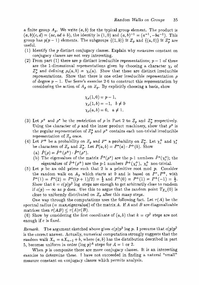
a finite group Ap • We write (a,b) for the typical group element. The product is(a, b)(c, d) == (ac, ad + b), the identity is (1,0) and (a, b)-1 == (a-I, -ba-I). Thisgroup has p(p - 1) elements. The subgroups {(I, b)} ~ Zp and {(a, O)} ~ Z; areuseful.(1) Identify the p distinct conjugacy classes. Explain why measures constant .on
conjugacy classes are not very interesting.(2) From part (1) there are p distinct irreducible representations; p - 1 of these
are the I-dimensional representations given by choosing a character Xi ofZ; and defining Pi(a,b) == Xi(a). Show that these are distinct irreduciblerepresentations. Show t~at there is one other irreducible representation Pof degree p - 1. Use Serre's exercise 2-6 to construct this representation byconsidering the action of Ap on Zp. By explicitly choosing a basis, show
Xp(I,O) == p - 1,
Xp(I,b)==-I, bf=O
Xp(a,b)==O, af=I.
(3) Let p+ and p* be the restriction of p in Part 2 to Zp and Z; respectively.Using the character of p and the inner product machinery, show that p* isthe regular representation of Z; and p+ contains each non-trivial irreduciblerepresentation of Zp once.
(4) Let P+ be a probability on Zp and P* a probability on Z;. Let xt and xibe characters of Zp and Z;. Let P(a, b) = P*(a) · P+(b). Show
(a) F(p) = P+(p+) · F*(p*).(b) The eigenvalues of the matrix F*(p*) are the p-I numbers P*(xi); the
eigenvalues of P+(p+) are the p-I numbers P+(xt), xt non-trivial.(5) Let p be an odd prime such that 2 is a primitive root mod p. Consider
the random walk on A p which starts at 0 and is based on P*, P+, withP*(I) == P*(2) == P*((p + 1)/2) = t and P+(O) == P+(I) == P+( -1) == t.Show that k == c(p)p2 log steps are enough to get arbitrarily close to randomif c(p) ~ 00 as p does. Use this to argue that the random point TXn (0) isclose to uniformly distributed on Zp after this many steps.One way through the computations uses the following fact. Let r(A) be the
spectral radius (== maxleigenvaluel) of the matrix A. If A and Bare diagonalizablematrices then r(AB) ~ r(A)r(B).(6) Show by considering the first coordinate of (a, b) that k == cp2 steps are not
enough if c is fixed.
Remark. The argument sketched above gives c(p)p2 log p. I presume that c(p)p2is the correct answer. Actually, numerical computation strongly suggests that therandom walk X n = aXn - 1 + b, where (a, b) has the distribution described in part5, becomes uniform in order (log p)A steps for A = 1 or 2.
When p is composite there are more conjugacy classes. It is an interestingexercise to determine these. I have not succeeded in finding a natural "small"measure constant on conjugacy classes which permits analysis.
36 Chapter 3D
D. RANDOM TRANSPOSITIONS: AN INTRODUCTION TO THE REPRESENTATION
THEORY OF THE SYMMETRIC GROUP.
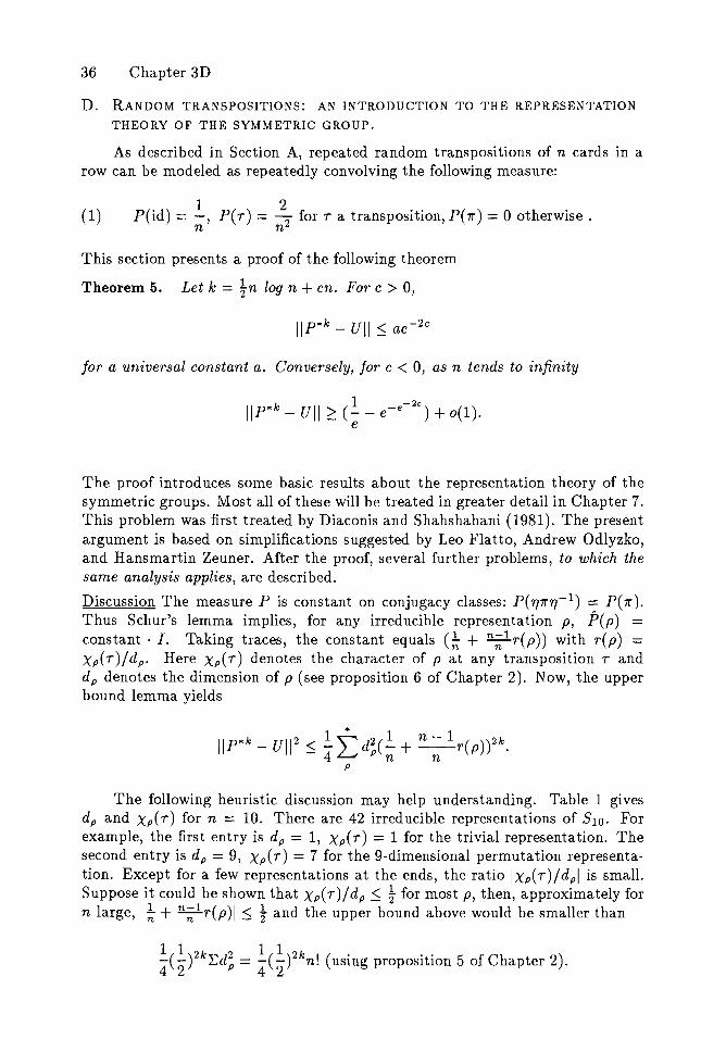
As described in Section A, repeated random transpositions of n cards in arow can be modeled as repeatedly convolving the following measure:
(1) P(id) = .!., Per) = ~2 for r a transposition, P(1r) == 0 otherwise.. n n
This section presents a proof of the following theorem
Theorem 5. Let k = tn log n + en. For e > 0,
for a universal constant a. Conversely, for c < 0, as n tends to infinity
k 1 -2cIIP* - UII ~ (- - e-e ) +0(1).e
The proof introduces some basic results about the representation theory of thesymmetric groups. Most all of these will be treated in greater detail in Chapter 7.This problem was first treated by Diaconis and Shahshahani (1981). The presentargument is based on simplifications suggested by Leo Flatto, Andrew Odlyzko,and Hansmartin Zeuner. After the proof, several further problems, to which thesame analysis applies, are described.
Discussion The measure P is constant on conjugacy classes: P(TJ1rTJ-l) = P(1r).Thus Schur's lemma implies, for any irreducible representation p, p(p) =constant · I. Taking traces, the constant equals (~ + n~1 r(p)) with r(p) =Xp(r)/d p. Here Xp(r) denotes the character of p at any transposition randdp denotes the dimension of p (see proposition 6 of Chapter 2). Now, the upperbound lemma yields
The following heuristic discussion may help understanding. Table 1 givesdp and Xp(r) for n == 10. There are 42 irreducible representations of S10. Forexample, the first entry is dp == 1, Xp(r) == 1 for the trivial representation. Thesecond entry is dp == 9, Xp(r) == 7 for the 9-dimensional permutation representation. Except for a few representations at the ends, the ratio IXp(r)/dpl is small.Suppose it could be shown that Xp( r)/dp ~ t for most p, then, approximately forn large, I~ + n~1 r(p)1 ~ t and the upper bound above would be smaller than
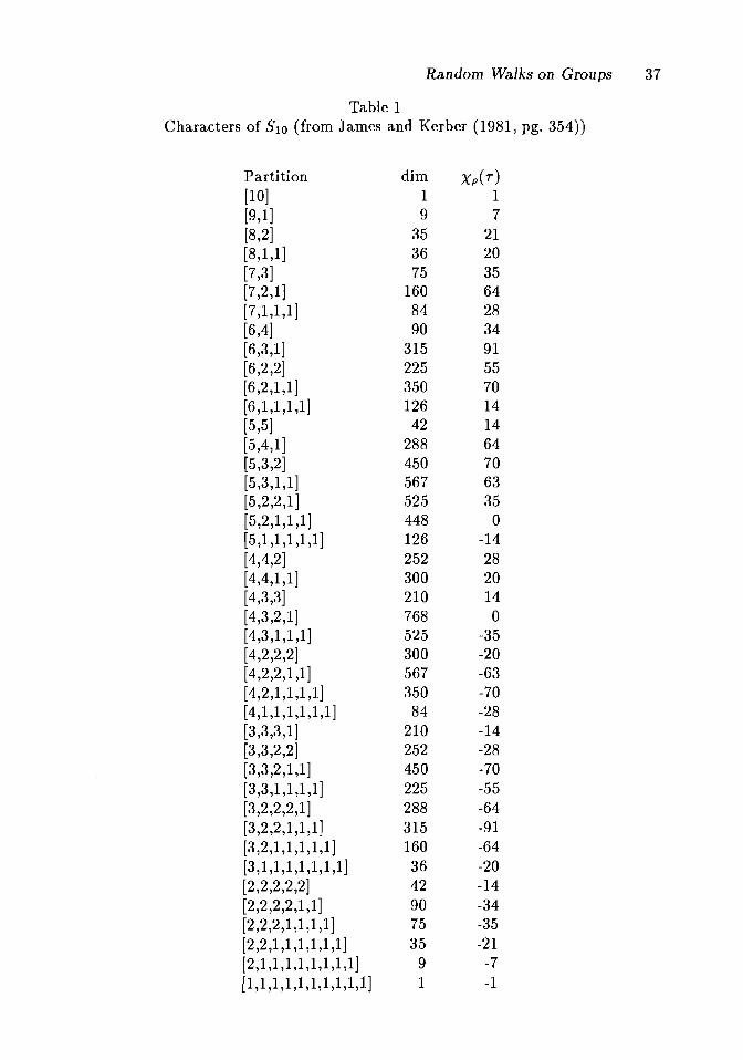
Random Walks on Groups 37
Table 1Characters of BIO (from James and Kerber (1981, pg. 354))
Partition dim Xp(r)[10] 1 1[9,1] 9 7[8,2] 35 21[8,1,1] 36 20[7,3] 75 35[7,2,1] 160 64[7,1,1,1] 84 28[6,4] 90 34[6,3,1] 315 91[6,2,2] 225 55[6,2,1,1] 350 70[6,1,1,1,1] 126 14[5,5] 42 14[5,4,1] 288 64[5,3,2] 450 70[5,3,1,1] 567 63[5,2,2,1] 525 35[5,2,1,1,1] 448 0[5,1,1,1,1,1] 126 -14[4,4,2] 252 28[4,4,1,1] 300 20[4,3,3] 210 14[4,3,2,1] 768 0[4,3,1,1,1] 525 -35[4,2,2,2] 300 -20[4,2,2,1,1] 567 -63[4,2,1,1,1,1] 350 -70[4,1,1,1,1,1,1] 84 -28[3,3,3,1] 210 -14[3,3,2,2] 252 -28[3,3,2,1,1] 450 -70[3,3,1,1,1,1] 225 -55[3,2,2,2,1] 288 -64[3,2,2,1,1,1] 315 -91[3,2,1,1,1,1,1] 160 -64[3,1,1,1,1,1,1,1] 36 -20[2,2,2,2,2] 42 -14[2,2,2,2,1,1] 90 -34[2,2,2,1,1,1,1] 75 -35[2,2,1,1,1,1,1,1] 35 -21[2,1,1,1,1,1,1,1,1] 9 -7[1,1,1,1,1,1,1,1,1,1] 1 -1

38 Chapter 3D
Now using Stirling's formula,
It follows that if k is n log n, the upper bound will tend to zero. To completethis heuristic discussion, consider the term arising from the n - 1 dimensionalrepresentation: dp = n -1, and Xp(r) = n - 3. This is easy to see: the traceof the permutation representation for a transposition is n - 2. The permutationrepresentation is the direct sum of the trivial representation and the n - 1 dimensional representation so n - 2 = Xp(r) + 1. Here (~+ n~Ir(p))2k = (1- ~)2k.
This is a far cry from (t )2k. Persevering, in the upper bound lemma k has to bechosen large enough to kill
(n - 1)2(1- ~)2k = e2k log(1-:-)+2 109(n-l) = e-~+2 log n+O(-!-r).n
For k = tn log n + en this is asymptotic to e- 4c• Taking square roots gives the
e-2c of the theorem.It will turn out that this is the slowest term, the other terms being geomet
rically smaller, and most terms being smaller than (t )2k.This argument is somewhat similar to the bounds for simple random walk on
Zp: terms near the trivial representation needed to be summed up carefully, termsfar away were geometrically small and easily dealt with. Putting in the details forZp required properties of cosine. For the symmetric group, the representationsare usefully thought of as 2-dimensional shapes. Properties of dp and Xp( r) willhave to be developed.
To begin a more detailed discussion, consider a partition of n, say A =(AI, .. . Am) with Al ~ A2 ... ~ Am positive integers with Al + ... + Am = n.There is a one to one correspondence between irreducible representations of Snand partitions of n. This is carefully described in Chapter 7. For present purposes, the notion of the diagram associated to a partition is helpful. An examplesays things best: the diagram corresponding to (5,3,1,1) is
The first row of the diagram contains Al squares, etc. A diagram containingnumbers 1, 2, ... , n is called a tableaux. Two tableaux are considered equivalentif they have the same row sets:
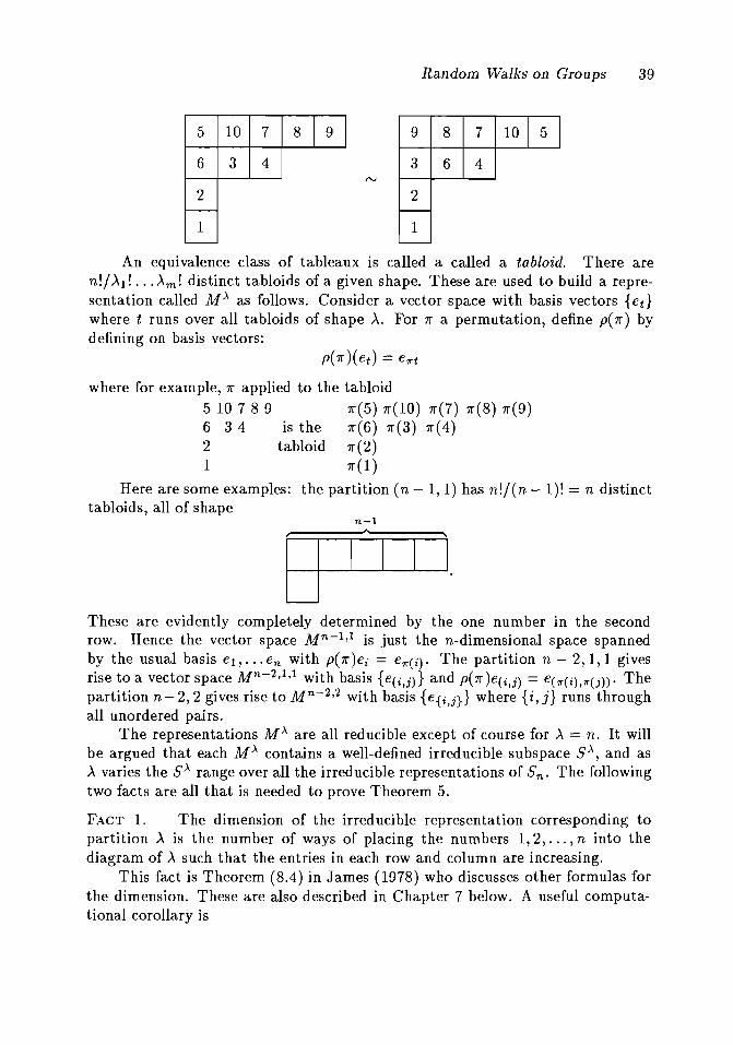
5 10 7 8 9
634
2
1
Random Wall,s on Groups 39
9 8 7 10 5
364
2
1
An equivalence class of tableaux is called a called a tabloid. There aren! / A1! ... Am! distinct tabloids of a given shape. These are used to build a representation called M.A as follows. Consider a vector space with basis vectors {et}where t runs over all tabloids of shape A. For 1r a permutation, define p(1r) bydefining on basis vectors:
where for example, 1r applied to the tabloid
5 10 7 8 9 1r(5) 1r(10) 1r(7) 71"(8) 71"(9)6 3 4 is the 71"(6) 1r(3) 1r(4)2 tabloid 71"(2)1 1r(1)
Here are some examples: the partition (n - 1,1) has n!/(n - I)! == n distincttabloids, all of shape
These are evidently completely determined by the one number in the secondrow. Hence the vector space Mn-1,1 is just the n-dimensional space spannedby the usual basis e1, . .. en with p( 1r )ei == e7t"(i)' The partition n - 2, 1, 1 givesrise to a vector space Mn-2,1,1 with basis {e( i,j)} and p( 71" )e( i,j) == e( 7t"( i),rr(j))' Thepartition n-2, 2 gives rise to Mn-2,2 with basis {e{i,j}} where {i,j} runs throughall unordered pairs.
The representations MA are all reducible except of course for A == n. It willbe argued that each MA contains a well-defined irreducible subspace SA, and asA varies the SA range over all the irreducible representations of Sn' The followingtwo facts are all that is needed to prove Theorem 5.
FACT 1. The dimension of the irreducible representation corresponding topartition A is the number of ways of placing the numbers 1,2, ... , n into thediagram of A such that the entries in each row and column are increasing.
This fact is Theorem (8.4) in James (1978) who discusses other formulas forthe dimension. These are also described in Chapter 7 below. A useful computational corollary is
40 Chapter 3D
(D - 1) The dimension d). of the irreducible representation corresponding
to the partition A satisfies d). :s; (~1 )d).* with A* ==
(A2' A3, ... , Am) a partition of n - Al.
Proof The first row may be chosen in (~1) ways. For each choice of first row, thenumber of ways of placing the n - Al remaining numbers is d)..*. Of course not allof these combine with the choice of first row to give a monotone total placement.This gives the inequality. 0
FACT 2. Let r(A) == x).(r)/d). where x)..(r) is the character at a transpositionand d). is the dimension of the irreducible representation corresponding to thepartition A of n. Then
(D - 2)1 2 1 ,""",).. ).'.
reA) = n(n _ 1)~[Aj - (2j - l)Aj] = (2) ~(2') - (2')J
with A' the transpose of A.
This is a special case of a result due to Frobenius who essentially determinedformulas for all of the characters. These become unwieldly for complex conjugacyclasses. An accessible proof of (D-2) is given in Ingram (1950).
Using Frobenius' formula, Shahshahani and I proved a simple monotonicityresult: Call partition Al larger than partition A2 if it is possible to get from thediagram of A2 to the diagram of Al by moving boxes up to the right. This is apartial order. For example (5, 1) 2: (4, 2) 2: (3, 3), but (3, 3) and (4, 1, 1) are notcomparable, though both are larger than (3,2,1). This order is widely used instatistics under the name of majorization (see e.g. Marshall and Olkin (1979)).James (1978, pg. 8) contains further examples.
LEMMA 1.(D-2).
If A 2:: A', then r(A) ~ r(A' ) where r(A) = x).(r)/d). is given by
Proof It suffices to consider the case where one box is switched from row b toa(b > a), Le. Aa = A~ +1, Ab == A~ - 1, Ac = A~ for c =I a, b. Formula (D-2) shows·that
1reA) - reA') = n(n _ 1)p; - (2a - l)Aa - A~ + (2a - l)A~+
A~ - (2b - l)Ab - A~2 + (2b - l)A~}
1 {' ( In(n-1) 2Aa +l- 2a-l)-(2Ab- 1)+(2b-l)}
1 {' I } 4( ) Aa - Ab +b - a +1 ~ ( ) > 0nn-1 nn-1
since A~ 2: A~ and b - a 2: 1. This argument is correct even if Ab = o. 0
LEMMA 2.
(a)
(b)
Random Wall(s on Groups 41
Let .A be a partition of n. Then
reA) ~ 1 - 2(n ~(:~~l)+ 1) if Al ~ n/2,
reA) ~ Al - 1.n-I
Proof·(a) By assumption .A ~ (.AI, n - .AI), so it follows from Lemma 1 and (D-2) that
1 22 2reA) ~ n(n -1) {Al - Al +n - 2nAl +Al - 3n +3AIl
2(Ai+A1- nAl- n)= 1 + ----------...-..-.----
n(n - 1)= 1 _ 2(Al + 1)(n - Al)
n(n - 1)m m m
(b) reA) = n(nl_l) ~ (A; - (2j - l)Aj) ~ n(n1_l) ~ Aj(Aj - 1) ~ n(~=~) ~ Aj =J=1 J=l J=1
Al-1 0n-l·
COROLLARY. Let A be such that reA) 2: o. Then
1 n - 1 { 1 _ 2(Al+l~n-Al)I; + -n-r(A)1 ~ ~ n
n
if .AI ~ n/2for all .A.
Proof of Theorem 5: If At denotes the transpose of A we certainly have eitherreA) ~ 0 or r(At) > 0, because XA = -X~ (see James 1978, p. 25). Hence
( )
2k ( ) 2k2 1 n-l * 2 1 n-1~~d). ;; + -n-r(A) ~ L d). ; + -n-r(A)
'\:r('\)?:O
( )
2k* 2 1 n-I t+ L d). ;; - -n-r(A )A:r(A»O
,,* 1 n - 1~ 2 LJ d~l- + __r(A)1 2k
.n n
A:r('\)20
For A = (n), which is contained in the next to last, but not the last sum, thisused
2 1 n - 1 2k 2 1 n - 1 2kd 1- - --r(n)1 + d( _ )1- - --r(n - 1,1)1
n n n n 1,1 n n
= (1- ~)2k + (n -1)2(1- !)2k ~ (n _ 1)2(1- ~)2kn n n
2 n - 1 2k= dn-1lI + --r(n - 1,1)1 ·n
42 Chapter 3D
In order to bound this sum we split it into two parts according as'xl ~ (l-a)n(where a E (0, t) will be chosen below)
2:* dl (~+ n: 1 r(A))2k =t 2: dl (~+ n: 1r(A))2kA:r(A)~O j=1 A:r(A)~O
A1=n-j
<~("!') n! (_ 2j (n_ j +1))2k ~(n) n! ( j)2k- L-t J ( 0)' 1 2 + L-t j (n _ )O)! 1 - -:;; .
j=1 n -) . n j>an
To obtain this we used the corollary to (D-2) above and
(where the A' are the irreducible representations of Sn-i).In order to give a bound for the first sum shown in (*) above recall that
k - !!.log n + en·- 2 ,
an""(1!') n! -4k( ~- j:2
j)
~ J (n_j)!eJ=1
an ( 1)'2 .> 2. -4k/n. "" n - . . -2 log n o(1- *")(j-1)_ n e L-t ( _ 0)'2 0' e ,. n ).).
J=1
we observe that the factor in front of the sum is exactly e-4c and so all we have. an 2(j-1) Loan 2j(j-l)
to do IS to bound E _n_._,-. n-2(1- n )(J-1) == E ~. n n for large values ofj=1 Jo j=1 Jo
n. The ratio between two consecutive terms in this sum is j~l . n4j /n, which, asa function of j, is decreasing if j < In and increasing if j > In. So if
4 og n 4 og nboth the first and the last ratio are less than q < 1 we may bound the sum by1~q. But the first ratio is < 1 if n ~ 17 and the last one is < 1 if a
1n n 4a < 1, Le.
n > (~)1/1-4a. This works well if a < 1/4.Now let's consider the second sum
The factor in front of the sum is ~ e-4c if n ~ 7 and a is close enough to t.Hence it is sufficient to bound the sum for large values of n. The ratio betweentwo consecutive terms is
(n.- j)2 (1- _1_0
)n log n,)+1 n-)
Random Walks on Groups 43
which is decreasing in j. So, if the first of these ratios,
(n - an)2 (1 l)n log n (1- a)2 1---.1-.- < n I-aan + 1 n - an - a
is less than one (this happens if n ~ ((1_",,)2) (1:0») we may bound the sum by ntimes the first term, that is, by
,n . (n) n. . (1 _ a)n log n.
an (n - an)!
Using Stirling's formula one can show that this tends to 0 (very slowly) if n tendsto 00 and so it must be bounded. This completes the proof of the upper boundpart of Theorem 5.
The following argument for the lower bound produces an explicit set A wherethe variation distance is large. Intuitively, if not enough transpositions have beenmade, there wil~ be too many cards that occupy their original positions. Let A bethe set of all permutations with one or more fixed points. Under U, the chance ofone or more fixed points is well known under the name of the matching problem.Feller (1968, Sec. IV.4) implies
1 1U(A) = 1 - - + Q( -).
e n!
To bound P*k(A), consider the process for generating p*k using randomtranspositions (L1 , RI)' ... , (Lk, Rk). Let B be the event that the set of labels{Li, Ri}f=l is strictly smaller than {I, ... , n}. Clearly A :) B. The probabilityof B is the same as the probability that when 2k balls are dropped into n boxes,one or more of the boxes will be empty. Arguments in Feller (1968, Sec. IV.2)imply that the probability of B equals .
-2k/n1 - e-ne +0(1) uniformly in k, as n -+ 00.
With k == ~n log n +en, P*k(A) ~ 1 - e-e-2c
+o(1). Thus
IIp*k - UII ~ IP*k(A)'- U(A)I ~ (P*k(A) - U(A))1 -2c
~ (- - e- e ) +o(1).e
o
Remarks.1) On Lower Bounds. The argument for the lower bound is satisfying in that
it produces a simple set that "explains" why tn log n steps are needed. Onthe other hand, the computation involved two classical results which wouldnot generally be available for other random walk problems. It is therefore of
44 Chapter 3D
some interest to see how the general approach to lower bounds works out inthis case.The general approach begins with the upper bound argument and chooses
the difficult or "slowest" representations to construct a random variable to workwith. In the present case, the difficult representation is sn-l,l. A reasonablecandidate for a random variable is thus the character X of this representation.Observe that this is exactly the number of fixed points minus one. Under theuniform distribution
1 2 IEU(X(1I")) = 0, Varu(x) = fGf~1rX (11") = (X X) = 1.
Under the convolution measure, with p the n - 1 dimensional representation,
Observe that in order to drive this to its correct value zero, k must betn log n+en for e large. However, this is not enough to lower bound the variationdistance since there are random variables with large means which are small withhigh probability. A second moment is needed. To compute this E k (X2 ) is needed.Now X2 is the character of the tensor product of X with itself. It is not difficultto argue that
sn-l,l ® sn-l,l = sn Ee sn-l,l E9 sn-2,2 E9 sn-2,l,l
dim (n - 1)2 1 n - 1 n(n2-3) (n-l)i n - 2 )
An explicit proof of this result can be found on page 97 of James and Kerber(1981).
EXERCISE 13. Using the data above, compute Vark(X) and use Chebychev'sinequality to show that tn log n - en steps are not enough.
2) While limited, the approach developed above gives precise results for someother problems. To begin with, consider random transpositions. The identity is chosen much more frequently than any specific transposition. It isstraightforward to carry out the analysis for the probability
If Pn = 1/(1 + (2))' all possible permutations are equally likely. In thiscase the argument shows that k = e(n)n2 transpositions are needed wheree(n) ~ 00 with n. This is somewhat surprising; usually, for a given supportset, the probability that approaches the uniform most rapidly is uniform onthe support set.Similarly, any simple probability on Sn which is constant on conjugacy classes
can be worked with. A key tool is a uniform bound on° the characters developed byVershik and Kerov (1981). A readable account of this is given by Flatto, Odlyzkoand Wales (1985). They work out details for probabilities uniform on a fixedconjugacy class e (e.g., all 3 cycles). Their results imply that tn log n steps are
Random Wall{s on Groups 45
always sufficient. This is not surprising - choosing a random 3-cycle mixes morecards each time and should result in faster convergence.
A simple problem not covered by available techniques is the rate of convergence for a random involution (1r 2 = id).· There are ~pdp of these, which isasymptotically (; )n/2 · eVn/V2e t. For this and other properties of involutionssee Stanley (1971, pg. 267). Such a measure is constant on conjugacy classes, butthe asymptotics haven't been worked out. It is not hard to show that any nontrivial conjugacy class generates Sn' See Arad and Herzog (1985). Thus there aremany open problems.
Finally, it is straightforward to handle random walks based on measuresconstant on conjugacy classes of the alternating group An. The characters of Anare available as simple functions of the characters of Sn' James and Kerber (1981)Chapter 2 give these results.
EXERCISE 14. Let n be odd. Let Q be uniform on the set of n cycles in An.Show that Q*2 is close to uniform for large n. (Hint: See formula 2.3.17 in Jamesand Kerber (1981) or Stanley (1983).)
3) Connections with Radon Transforms. The analysis developed in this sectionhas been applied to the study of uniqueness and inversion of the Radontransform by Diaconis and Graham (1985a). Here is a brief description: letG be a group with des, t) a bi-invariant metric: d(rs, rt) = d(sr, tr) = des, t).Let I: G ~ IR be a function. Suppose we are told not I(s) but
/(s) = L J(t) for all s and fixed a.d( s,t) $a
When do these averages determine I? If S = {s: d(id, s) ~ a} the Radontransform is l(s) = 15* f( s). Taking Fourier transforms, the Radon transformis unique if and only if is(p) is invertible for every irreducible representationp.The study of this problem leads to interesting questions of probability and
computational complexity even for groups as simple as Zr. In this case, with das Hamming distance, when a = 1, f --t I is 1 - 1 iff n is even; when a = 2, iff nis not a perfect square; for a 2:: 4 iff n is not in a finite set of numbers.
John Morrison (1986) derived exact results for this problem using Gelfandpair tools (Section F below). Jim Fill (1987) gives comprehensive results for Zn.For applications to data analysis, see Diaconis (1983). For general background,see Bolker (1987).
For G = Sn, choose d( 1r , 'fJ) as the minimum number of transpositions neededto bring 1r to 1]. This metric is further discussed in Chapter 6-B. For any biinvariant metric, Is is constant on conjugacy classes, so is(p) = cl. For a =l,c = (1+(2') rep)). Diaconis and Graham use this result and Frobenius' formulafor r(p) to argue that f ~ 7 is invertible iff n E {I, 3, 4,5,6,8, 10, 12}.
4) Perfect codes. Very similar computations occur in a seemingly different problem treated by Rothaus and Thompson (1966). Let G be a group and T be asubset of G. Say that T divides G if there is a set S in G such that each 9 E G
46 Chapter 3D
has a unique representation st == 9 with s in Sand t in T. For example, ifT is a subgroup, then T divides G. If G == 8 3 and T == {id, (12), (13), (23)},then T does not divide 8 3 •
The construction of codes leads naturally to questions of divisibility: Let Gbe a group and d(s,t) a G invariant metric on G (Le., d(s,t) == d(gs,gt)). Forexample, G might be Z2 and d might be the Hamming distance, or G might beSn and d( s, t) might be Cayley's distance: the minimum number of transpositionsrequired to bring s to t (see Chapter 6-B).
A subset S C G is called a code; S corrects k errors if any two code wordsare at distance more than 2k apart; 8 is perfect if G is the disjoint union of ballsof fixed radius centered at the elements of 8.
Perfect codes are elegant efficient ways of coding data with minimum waste.On Z2 the perfect codes have been classified; see MacWilliams and Sloane (1977).The search for codes in other groups is an active area of research.
To see the connection with group divisibility, consider Sn with Cayley's distance. Take T to be a (solid) ball of radius k about the identity. Observe that Tdivides Sn if and only if there is a perfect code S of this radius - indeed, ballscentered at points of S would be disjoint if T S == Sn uniquely.
Rothaus and Thompson considered k == 1, Le. T as the identity togetherwith the set of all transpositions in Sn' To explain their result, observe that anecessary condition for divisibility is (1 + (2') )In! (after all, disjoint balls of radius1 have to cover). This rules out n == 3,4,5 but not 6 for example. They provedthat if (1 + (2)) is divisible by a prime exceeding vn+2, then T does not divideSn.
Their argument is very similar to the argument for analyzing repeated random transpositions. Interpret the equation ST == G as an equation about theconvolution of the indicator functions of the sets Sand T(ls * IT = 1 say). Taking Fourier transforms at an irreducible representation leads to c(p)js(p) = 0,where c(p) = 1 + (2')Xp(r)/dp. Now one must study when c(p) vanishes (see theprevious remark). One really new thing in the Rothaus-Thompson paper is theskillful use of transforms at non-irreducible representations to give checkable divisibility constraints on n. The argument is fairly detailed and will not be givenhere. Sloane (1982) connects this work with the modern coding literature andgives many further applications. Chihara (1987) extends the results to Chevalleygroups.
EXERCISE 15. Rothaus and Thompson report 1,2,3,6,91, 137,733, and 907as the only integers less than 1,000 which fail to satisfy the theorem. The naivecriterion does 3, (and 8 2 is divisible). Show that 8 6 is not divisible.
5) Varying the measure. The ideas developed above can be used for some related problem like transpose a random card with the top card, or switch thetop k cards with k randomly chosen cards. Here we have a measure on Sninvariant under conjugation by Sk and bi-invariant under Snk. The Fouriertransform can be shown to be diagonal with explicitly computable elements.See Diaconis (1986) or Greenhalgh (1988) for further details.
6) Random reflections. Similar analyses are possible for other random walks
Random Walks on Groups 47
constant on conjugacy classes. For example, let G == Gp - the p-dimensionalorthogonal group. One practical problem involves algorithms for choosing arandom element of G when p is large (e.g. p = 256). The usual algorithmbegins with p2 standard normal random variables Xij, forms a matrix M =={Xij} and makes M orthogonal using the Gram-Schmidt algorithm. It is easyto show that this results in a random orthogonal matrix uniformly distributedon G. Diaconis and Shahshahani (1987a) discuss this and other algorithms.In carrying out the Gram-Schmidt algorithm, the ith row of M must bemodified by subtracting out the inner product of all rows above it. Thisentails computation of i-I inner products. Each inner product involves p
p
multiplications and additions. The whole procedure takes order p L: i ==i=l
O(p3) operations. This is often too large for practical use.Sloane (1983) contains a fascinating application to encrypting telephone conversations. Sloane suggested generating a matrix by using random reflections.Geometrically this involves choosing a random point U in the p-sphere andreflecting in the hyperplane orthogonal to U. Algebraically the matrix isf == (I - 2UU'). Observe that the distribution of r is constant on conjugacyclasses because fI(l - 2UU')r~ == (1 - 2rI U(r1U)'). If U is uniform on thep-sphere, r 1 U is uniform as well. There is a straightforward extension of theupper bound lemma to compact groups. The analysis can be carried out toshow that tp log p + cp steps are enough (while tp log p - cp steps are toofew). Some details can be found in Diaconis and Shahshahani (1986a).In this problem, P is singular with respect to the uniform distribution, butp*k has a density for k 2: p. Thus variation distance bounds make sense. Forrandom walks on continuous compact groups involving a discrete measure,the distribution is always singular and only bounds in a metic for the weakstar topology can be hoped for.
7) Random walks on linear groups over finite fields. The problem describedabove can be carried out over other fields such as C (to generate a randomunitary matrix) or Fq - a finite field with q == pd elements. Here is anotherproblem which should lead to interesting mathematics. Let V be a vectorspace of dimension d over Fq • Let SLd(V) be the dxd invertible matrices with
determinant 1. This is a finite group of order q(g)IIf=2(qi -1). A transvectionis a linear transformation in S Ld(V) which is not the identity but fixes allelements of a hyperplane. Suzuki (1982, Sec. 9) shows that if d 2: 3, thetransvections form a single conjugacy class that generates SLd(V). Thus,the question "how many random transvections are required to get close tothe uniform distribution on S Ld(V)?" can be attacked by the method of thissection.
48 Chapter 3E
E. THE MARKOV CHAIN CONNECTION.
1. INTRODUCTION.
There is another approach to random walks on groups: treat them as Markovchains with state space G and IGI X IGI transition matrix Q(s, t) = Q( ts- I
).
In early attempts to understand the problem of random transpositions JosephDeken did exact computations of the second largest eigenvalue for decks of sizen = 2, 3, ... ,10. He found it to be (1 - 2/n). This is precisely the constant inthe Fourier transform at the "slow" representation (see Theorem 5 of Section D)..This striking numerical coincidence suggested that (a) the (1 - 2/n) result musthold for all n, and (b) there is a close connection between the Markov chain andgroup representation approach. Some of this was worked out by Diaconis andShahshahani (1981), who showed that the eigenvalues of the transition matrix areprecisely the eigenvalues of Q(p), each appearing with multiplicity dp •
The following discussion uses work of Matthews (1985). It results in a sort ofdiagonalization of the transition matrix and an exact determination of eigenvaluesand eigenvectors where these are available. This allows us to use results fromclassical Markov chain theory.
2. A SPECTRAL DECOMPOSITION OF THE TRANSITION MATRIX.
Let G be a finite group with elements {SI,.'" SN}, N = IGI. For a probabilityQ on G, construct Q(i,j) = Q(SjS;I) - the chance that the walk goes from Sito Sj in one step. Suppose that the irreducible representations are numberedPI,·· ., PI(· Define
(1)
a d~ X d~ block matrix with Q(Pk) the Fourier transform of Q at Pk.
(2) Let M be the N X N block diagonal matrix (MI 0 )
o MI(
Suppose that a basis has been chosen so that each irreducible representationis given by a unitary matrix. Define
a column vector of length d~. Let <p(s) = ('l/Jl(s)T,'l/J2(S)T, ... ,'l/J/«s)T)T be acolumn vector of length N obtained by concatenating the 'l/Jk( s) vectors.
(4) Let <p be the N X N matrix (<p(St), ... ,4J(SN)) and 4J* its conjugate
transpose.
Random Wall,s on Groups 49
Theorem 6. The transition matrix Q( i, j) can be written
(5) Q = ~*Af*~
Remarks. The Schur orthogonality relations show that ~ is a unitary matrix.So (5) is a decomposition similar to the traditional eigenvalue, eigenvector decomposition. It implies that each eigenvalue of tJ(p) is an eigenvalue of Q( i, j)with multiplicity dp. Together these are all the eigenvalues of Q( i, j). If Af isdiagonal (e.g. Q constant on conjugacy classes or bi-invariant on a Gelfand pair(Section F below)), then (5) is the spectral decomposition of Q with respect toan orthonormal basis of eigenvectors.
Proof of Theorem 6: The Fourier inversion theorem gives
1 K 1 KQ(i,j) = N LdkTr[Q(Pk)Pk(Si)Pk(sjl)] = N LdkTr[Pk(sjl)Q(Pk)Pk(Si)].
k=l k=l
Expanding the trace, this equals
!(
L 'l/Jk(Sj)* Mk'l/Jk(Si)'k=l
o
3. THE FIRST HIT DISTRIBUTION.
Let G be a finite group and Q a probability on G. For s, t E G, defineFit = the probability that t is first hit at time n starting at s. For Izl < 1 let
00
Fst(z) = L: F:t zn .n=l
Theorem 7. For Izl < 1, (1 - zQ(p)) is invertible and
Fst(z) = ~pdpTr[p(srl)(1 -=- zQ(p»-l] .I;pdpTr[I - zQ(p)]-l
00
Proof. Using the notation of Section 2, Q(z) = L: znQn = {4J*(I - zM*)-l4J}.n=!
Kemperman (1961, pg. 18-19) gives the standard result
The result follows from this and (5) above. It is given a direct independent proof inSection H. It is mentioned here to underscore the availability of the Markov chainmachine in situations where all the eigenvalues and eigenvectors of the transitionmatrix are known.
50 Chapter 3E
4. ON GENERALIZED CIRCULANTS.
The technique we have developed for analyzing random walks gives rise toa class of "patterned matrices" for which we can explicitly determine all theeigenvalues and eigenvectors. Let G be a finite group of order g. Let 81, ... ,8g bean enumeration of the elements of G. Let P be a probability measure on G. Thetransition matrix associated with P is the 9 X 9 matrix with i, j entry P(s jS:;I).If a random walk on G is thought of as a Markov chain with G as state space, thei, j entry is the probability of a transition from state Si to state Sj' We have beenworking with measures which are constant on conjugacy classes. Generalizing thissomewhat define a G-circulant as a 9 X 9 matrix with i, j entry I( Sjs:;l) with fconstant on conjugacy classes.
Examples. If G is Abelian, then the equivalence classes consist of single elements. If G is cyclic, then a G circulant is an ordinary circulant: a 9 X 9matrix in which each row is a cyclic shift of the first row. For G = 53 theequivalence classes are {id}, {(1 2), (1 3), (2 3)}{(1 2 3), (1 3 2)}. If f(id) =a,f(l 2) = b,f(l 2 3) = c and the group is labelled in order (using (~~~)notation) (1 2 3)(1 3 2)(2 1 3)(2 3 1)(3 1 2)(3 2 1), we get
dim114
typical vector(1 1 1 1 1 1)(1 -1 -1 1 1 -1)(200 -1 -1 0)
valuea +3b + 2ca - 3b +2c
a-c
a b bee bb a ebb cb cab b cebb a c bebb cabbee b b a
Let G be the 8 element quarternion group G = {±1, ±i, ±j, ±k} with multiplicai
tion given by /' ~ .. Thus ij = k, kj = -i, etc. There are five conjugacy classes:k +-- J
{+l},{-l},{±i},{±k}. Let them have weight a, b, c, d, e. Label the group 1,-1, i, -i, j, -j, k, -k. We get
abccddeebaccddeeccabeeddccbaeeddddeeabccddeebacceeddccabeeddccba
valuea + b + 2c +2d + 2ea + b + 2c - 2d - 2ea + b + 2d - 2c - 2ea + b + 2e - 2c - 2d
a-b
typical vector(1 1 1 1 1 1 1 1)(1 1 11 -1 -1 -1 -1)(1 1 -1 -1 1 1 -1 -1)(1 1 -1 -1 -1 -1 1 1)(1 -1 0 0 0 0 0 0)
dim11112
Theorem 8. Let M be a G-circulant. Then M has an eigenvalue Ap for eachirreducible representation p of G,
Random Walks on Groups 51
the eigenvalue Ap occurs with multiplicity d~.
Proof. The spectral decomposition of Section 2 above proves a stronger result:it gives the eigenvectors as an explicit arrangement of the matrix entries of theirreducible representations.
Remarks.1. There is a lovely book called Circulant Matrices by Phillip Davis (1979). It
seems like a nice project to go through the book and generalize all the resultsto G-circulants.
2. Note that the character vector (Xp( SI) ... Xp( Sg)) is always an eigenvector forAp •
3. The argument generalizes easily to a transitive action of G on a finite set X. IfP is a probability on G, then P induces a Markov chain on X. The transitionmatrix of this chain has the same eigenvalues as the matrices Pep), where pruns over the irreducible representations of G that appear in the permutationrepresentation of G on X. This is developed in Section F which follo\vs.
4. Example 3 of Section C suggests some further extensions. This begins withthe Markov chain X n = 2Xn - 1+ En (mod p) with Ei LLd. taking values0, ±1 with probability t. The transition matrix M of this chain is not acirculant, but the argument shows that its ath power is a circulant, where ais the order of 2 (mod p). Thus one knows, up to an ath root of unity, all theeigenvalues of M. Remark 2 of the example suggests many further situationswhere a similar analysis is possible.
F. RANDOM WALKS ON HOMOGENEOUS SPACES AND GELFAND PAIRS.
1. HOMOGENEOUS SPACES.
There is an extension of the basic set up which is useful. It involves theMarkov chain induced by a random walk under the action of a group. This arisesin some of the introductory examples: for instance, in considering the recurrenceX n = an X n - 1 +bn X n - 2 (mod p), a random walk on 2 X 2 matrices was considered.The matrices act on pairs (Xn , X n - 1 ). To understand the behavior of X n it isnot necessary to bound the rate of convergence on the group of matrices, but onlyon the set of non-zero pairs. Similarly, the grand tour example in section A4 onlyinvolved the action of the orthogonal group on lines or planes.Definition. Let G be a finite group and X be a finite set. An action of G on Xis a mapping from G X X --+ X which we will denote (s, x) --+ s · x or simply sx.It must satisfy: id·x = x and S • (t · x) = (st) · x. Define an equivalence on Xby x rv y if for some s E G, sx = y. The equivalence classes are called orbits. Goperates transitively on X if there is only one orbit. A set with a group actingtransitively is called a homogeneous space.
When G operates transitively, the following canonical representation of Xis useful. Fix Xo EX. Let N - the isotropy subgroup of Xo - be the set ofs E G with sXo = xo. The group G acts on the coset space G/ N. There is anisomorphisim between X and G/ N respecting the action of G. We will identify

52 Chapter 3F
X with xo, xl, ... , X n , a set of coset representatives for N in G. It will always beassumed that Xo = id.
Example 1. The symmetric group Sn acts on {I, 2, .. . n} transitively. Theisotropy subgroup is isomorphic to Sn-l - as all permutations fixing 1. Cosetrepresentatives can be chosen as the identity and the transpositions (12), ... , (In).
A probability P on G induces a probability P on X = GIN by P(Xi) =P( Xi N ). Similarly, if p*k denotes the convolution of P with itself k times, p*kinduces a probability on X. We can think of a process with values in G, say id,81, 82 81, 83 8 2 81, .... The induced process in X is XO, 8IXO, S2 8 I X O,· •• •
EXERCISE 16. Let the finite group G act on the finite set X, partitioning Xinto orbits (Ji. If P and Q are probabilities on X which are G-invariant, then
Thus, the variation distance between P and Q equals the distance between theirrestrictions to the set of orbits. This is a special case of the following result: ifP and Q are probabilities on a a-algebra F and if a sub-a-algebra B C F issufficient for P and Q, then liP - QIIF = liP - QIIB. See Diaconis and Zabell(1982) for details and applications.
LEMMA 3. Let G act transitively on X. Let P be a probability on G. Theinduced process is a doubly stochastic Markov chain on X with transition matrixPx(y) = P(yNX-I).
Proof. For the induced processes, the chance of going from X to y in one step isPx(y) defined as P{s:sx = y} = P{yNx- I }. For a Markov chain, the chance ofgoing from x to y in two steps is of course
z
The chance that the chain in question is at y in two steps is
P * P(yN) = L P(yNs-1 )P(s).s
Let s = xn, we get
x,n x
The last computation is essentially the inductive step of a proof that the measureinduced by p*k on X equals P:o(y). 0
To state the next result, introduce L(X) - the set of all functions from Xinto the complex numbers. The action of G on X induces an action of G on L(X)
Random Walks on Groups 53
by sf(x) = f(s-lx). This is a 1 - 1 linear mapping of L(X), and so yields arepresentation of G. The representation splits into a direct sum of irreduciblerepresentations p.
LEMMA 4. (Upper bound lemma). Let G operate transitively on the finite setX. Let N be the isotropy subgroup. Let P be a right N invariant probability onG, P the induced probl6bility on X, and U the uniform distribution on X. Then
where the sum is over all nontrivial irreducible representations that occur inL(X).
Proof. Let (; be the uniform probability on G.
(~xIP(x) - U(x)I)2 :::; IXI~xIP(x) - U(x)12 == IXIINI~s(P(s) - U(s)(2
== ~;dpTr(P(p)P(p)*).
In the last step, the Plancherel theorem was used together with the facts that aright N invariant function has zero Fourier transform if p does not occur in L(X).This follows from the following lemma and remark. 0
LEMMA 5. Let p, V be an irreducible representation of the finite group G. LetN c G be a subgroup ~nd X = G/ N the associated homogeneous space. Thenumber of times that p appears in L(X) equals the dimension of the space of Nfixed vectors in p, V(= dim{ v E V: p(n)v = v for all n E N}).
Proof. Let {ox(')} be a basis for L(X). The character X for the representationof G on L(X) is
x(s) == ({x: 6x (s-ly) = 6x (y)}1 = I.x: sx = xl
== Ix: x-1sx E NI.
Now, the number of times p appears in this representation is
1 1(xplx) = iGi L Xp(s)X(s) = iGi L Xp(s)
s s
= I~I ~Xp(n) ~x-1sx=n
But, for any fixed n,
L l=IXI·s,x
x-1sx=n
1
To see this observe that for fixed n, x, s = xnx- 1 is determined. Further, ifx-1sx == n, then (tX)-ltst-1(tx) = n for all t E G. Since G operates transitivelyon X, for every y E X there is a unique s* such that y-l s*y == n.
54 Chapter 3F
Since IGI/IXI = 1Nl,
The right side is the number of times the trivial representation appears in XPrestricted to N. This is just the dimension of the space of N fixed-vectors. 0
Remarks. Lemma 5 is a special case of Frobenius' reciprocity formula. Therepresentation L(X) is the trivial representation of N induced up to G. Frobenius'formula says the number of times a representation p of G appears in the inductionof A (a representation of N) to G equals the multiplicity of A in p restricted toN. Chapters 3 and 7 of Serre (1977) give further development. The general resultis proved by essentially the same combinatorial argument. For present purposes,Lemma 5 is all that is needed.
Using Lemma 5, if p does not occur in L(X), the trivial representation doesnot occur in p restricted to N. Now, the orthogonality relations (Corollary 2 ofSchurs lemma in Chapter 2) yield ~nP(n) = o. For a right N invariant functionf on G,
j(p) = ~x f(x) p(x)~n pen) = o.This completes the proof of the upper bound Lemma 4.
The next section discusses a collection of examples where a huge simplificationoccurs.
2. Gelfand pairs
This is a class of examples where the Fourier analysis becomes simple. Consider, as above, a group G acting transitively on a finite set X with isotropysubgroup N. A function f: G ~ C is called N-bi-invariant if f(nlsn2) = f(s) forall s E G, nl ,n2 EN.Definition. G, N is called a Gelfand pair if the convolution of N hi-invariantfunctions is commutative.
One value of this definition comes from a long list of examples. Some of theseare discussed later in this section. Letac (1981, 1982) or Bougerol (1983) presentvery readable surveys of available results. The following theorem is basic:
Theorem 9. The following three conditions are equivalent(1) G, N is a Gelfand pair.(2) The decomposition of L(X) is multiplicity free.(3) For every irreducible representation (p, V) there is a basis of V such that
j(p) = (~g) (a matrix with zero entries except perhaps in the (1, 1) position)
for all N -bi-invariant functions f.
Proof Assume (2), so L(X) = VI 61 V2 61 ... 61 Vm say. This is multiplicity free, soby Lemma 5 above, each Vi has a non-trivial one-dimensional space of N invariantfunctions. Choose so called spherical functions Si E Vi to be left N -invariant and
Random Walks on Groups 55
normalized so si(id) = 1. Complete Si to a basis for Vi chosen so pi(n) = (~~)
for all n E N (the top block is 1 X 1, the bottom block is (d i - 1) X (d i - 1)).For / an N -bi-invariant function,
s x,n x n
But Pi restricted to N has a one-dimensional space of fixed vectors. By theorthogonality relations for the matrix entries, the (a, b) entry satisfies
L pib(n) = {1 N l if a = ~ = 1o otherwIse.
n
Thus ](Pi) has the form E/(x )(: 0) = (: 0). This argument works for any rightinvariant function I. For left invariant I, a similar argument shows that !(Pi)has form (......0·· ... ). From Lemma 5, if P does not appear in L(X), j(p) = o. Thisshows (2) implies (3).
Clearly (3) implies (1) by taking Fourier transforms. To finish off, suppose(1) but some Pi has multiplicity j > 1 in L(X). Pick a basis of Vi with first j coordinates spanning the N -invariant space. Take M 1 , M 2 any two non-commutingj X j matrices. Define /1, /2 on G by
By Fourier inversion, these are non-zero, N -bi-invariant functions and fl * 12 f;/2 * fl. 0
COROLLARY. Let (G, N) be a Gelfand pair with L(X) = VI EB ••. EB Vm • EachVi contains a unique N -invariant function Si with SiC id) = 1. If the Fouriertransform of an N invariant probability P on X is defined by
P(i) = Exsi(x)P(x),
then, for U the uniform distribution on X
IW~o - UI1 2 ~ l td i l.P(i)1 2k.
i=1
Remarks. The corollary follows from the theorem above and the upper boundlemma of the last section. The Si are called spherical functions. They have beenexplicitly computed for many groups. From part (3) of the theorem Si(X) =Pie X )11. This sometimes serves as a definition, or as a way of computing sphericalfunctions: take (pi, Vi), a unitary representation that appers in L(X). By the
56 Chapter 3F
theorem, Vi contains a one-dimensional space of N fixed vectors. Let u be a unitN-fixed vector. Then Si(X) =< pi(X)U,U >. The Si are left N invariant functionson X. They are also N-bi-invariant functions on G. Turning things around, ifthe spherical functions are known, the * in Theorem 9-3 can be computed asl: f( t)s( t).
tEG
EXERCISE 17. Let Xi be the character of a representation Pi that appears inL(X). Show
Thus the spherical functions are determined by characters.
3. Example: The Bernoulli-Laplace model of diffusion.
As a specific example of the techniques discussed above consider the followingmodel of diffusion suggested originally by Daniel Bernoulli and Laplace. Feller(1968, p. 378) contains the history. There are two urns, the first containing nred balls, the second containing n white balls. At each stage, a ball is picked atrandom from each urn and the two are switched. Evidently, many switches mixthings up and it is not difficult to show that once things reach equilibrium theyevolve (approximately) as an Ornstein-Uhlenbeck process (at least for large n).The problem is, how many switches are required to reach equilibrium? In whatfollows, we show that !J' log n + en switches suffice.
It is just as simple to solve the same problem with r red balls in the first urnand b black balls in the second urn. Let n = r + b. A convenient mathematicalmodel for this has X == Sn/ Sr X Sb; thus X can be thought of as the set ofr element subsets of a set with n elements. For x, y E X define the distanced(x, y) == r - Ix n yl. This is a metric (see Chapter 6-D), and the random walkproblem becomes the following: start at Xo == {I, 2, ... , r}. Choose an elementinside Xo and an element outside Xo and switch them. This chooses a set x atdistance one from Xo at random. The following result is proved by Diaconis andShahshahani (1987b).
Theorem 10. For nearest neighbor random walk on the r sets of an n set, ifk = ~(1 - ;) log n + er then
for positive universal constants a and d.
Proof. Without loss, take r :::; n/2. The space decomposes as L(X) = Vo EBVI EB · .. EB Vr where Vi is the irreducible representation of the symmetric groupSn corresponding to the partition (n - i, i). James (1978) gives this result as wellas dim(Vi) = (r) - (i~l). In particular, the pair (Sn,Sr X Sb) is a Gelfand pair.
The spherical functions have been determined by Karlin and McGregor (1961)in studying an equivalent formulation in a genetics example (Moran's model).Stanton (1984) contains this result in modern language. The spherical functions
Random Wall{s on Groups 57
turn out to be classically studied orthogonal functions called the Dual Hahn orEberlein polynomials. The function 8i(X) only depends on the distance d(x,xo)and is a polynomial in d given by
-(d) - ~ (-i)m(i - n - l)m( -d)m 0 .81, - L...J (_) (_)' ::; t ::; r,
m=O r n m r mm.
where (j)m = j(j + 1) ... (j +m-I). Thus,
1~dso(d) = 1, sl(d) = 1- ( )'rn-r
(d)- 1 _ 2(n - l)d (n - l)(n - 2)d(d - 1)
82 - + ·r(n-r) (n-r)(n-r-l)r(r-l)
The basic probability P for this problem is supported on the r(n - r) sets ofdistance one from the set {I, ... , r}. Thus the Fourier transform of P at the ithspherical function is
(3)" . i(n - i +1) .P( t) = si(l) = 1 - ( ) 0::; t ::; r.rn-r
Now the corollary to Theorem 9
lipk - unz ::; ~ t{(~) - (. n )Hl- i(n- i + 1))2k.4 i=l t t - 1 r(n - r)
To bound this sum, consider first the term for i == 1,
n 2k(n-l)(l- ( )).rn-r
This is essentially-~+ logne r(n-r) •
Thus k must be ~(1 - ;;) log n at least to kill this term. If r = n/2, this becomesi log r. If r = o(n), this becomes ~ log n.
Next consider the final term
((~) _ ( n ))(_1 )2k.r-l n-r
This is certainly bounded above by
nr_1_ _ -2k log ~+r log n- log r!
, (!1)2k - e ·r. 2
In any case, if k is of order ~(l - ~) log n, this tends to zero exponentiallyfast. The intermediate terms are always geometrically smaller than the extreme
58 Chapter 3F
terms, just as with the argument for random transpositions. Further details arein Diaconis and Shahshahani (1987b). 0
Remark 1. As described in Section E, the analysis gives a precise formula forthe eigenvectors and eigenvalues of the transition matrix of this problem treatedas a Markov chain. Karlin and McGregor (1961) essentially derived this resultwithout using group theory. Their application was to a similar problem arisingas a genetics model due to Moran. A clear discussion of Moran's model can befound in Ewens (1979, Sec. 3.3). Diaconis and Shahshahani give applications toa learning problem discussed by Piaget.
Remark 2. As usual with approximation, some precision has been lost to geta clean statement. The basic result is the bound of the corollary to Theorem 9.When r = 1 for example there is only one term: (n - 1)( n~I )2k. For k = 1 taking
square roots gives tV~-I as an upper bound for the variation distance. Elementary considerations show that the exact distance in this case is l/n. Here, whenn is large, use of the upper bound lemma gives the right answer for the numberof steps required (namely 1) to make the distance small but an overestimate forthe distance itself.
EXERCISE 18. Consider two urns, the left containing n red balls, the rightcontaining n black balls. At each stage "a" balls are chosen at random from eachurn and the two sets are switched. Show that this is bi-invariant. Show that forfixed a, as n ~ 00, this speeds things up by a factor of a (so 4
Ia n log n moves
suffice).
Remark 3. A reasonable number of other problems allow very similar analysis.Stanton (1984) contains a list of finite homogeneous spaces arising from Chevalleygroups where (a) the associated L(X) is a Gelfand pair, and (b) the sphericalfunctions are explicitly known orthogonal polynomials. One case of particularinterest is a walk in the set of r-dimensional subspaces of an s dimensional vectorspace over a finite field. See Greenhalgh (1988) for details. In all cases, there is anatural metric so that nearest neighbor walks on X allow a I-dimensional analysis.For the example of r-dimensional subspaces the distance is d(x, y) = r-dim(xny).
A special case of this analysis is nearest neighbor walk on the cube X = Z2.Here G can be represented as the semi-direct product of Z;r with Sn. This is thegroup of pairs (x,7t") for x E Z2' 7t" E sn. It acts on y E Z2 by (x,7t")(y) =7t"y +x. Multiplication in G is composition of repeated transformations. ChoosingXo = 0, the isotropy subgroup is N = {(0,1r):7t" E Sn} ~ Sn. It is easy toverify that L(X) = Vo EB VI EB ... EB Vn where Vj is the subspace spanned bythe functions {fy(x)}IYI=j and fy(x) = (_l)Xoy. Thus G, N is a Gelfand pairand dim Vj = ("]). The spherical functions S j(x) again only depend on d( x, 0)(with d(x, y) = #places(xi f:. Yi)) and are polynomials in d called I{rawtchoukpolynomials:
j
sj(d) = (~) L (-l)m(~)G:::J·J m=O
Random Walks on Groups 59
The upper bound found by treating this problem as a Gelfand pair is the same asthe upper bound by treating the problem on the group Z2' (Example 2 of SectionC).
Remark 4. The theory of Gelfand pairs can be developed without using grouptheory. One advantage of the present program is that it offers a route to follow forproblems where the representation is not multiplicity free. For example, considerthe Bernoulli-Laplace urn model with 3 urns; the first containing n red, the secondcontaining n white, the third containing n blue balls. At each stage, a pair of urnsis chosen at random, then a randomly picked pair of balls is switched. Analysisof the contents of even the first urn is complicated by the fact that the associatedrepresentation of S3n on L(X), with X == S3n/ Sn X Sn X Sn, has multiplicity.(See Young's rule in Chapter 7.) This is an open problem.
There is a useful sufficient condition for showing that (G, N) is Gelfand without explicitly determining the decomposition of L(X).
LEMMA 6. (Gel/and's lemma). Let r be 1 - 1 homomorphism r: G ~ G withthe property s-l E Nr(s)N for all s E G. Then (G, N) is a Gel/and pair.
Proof. Note first that for bi-invariant functions f(S-l) = f(r(s)) and r(N) C N.If f is bi-invariant, define 1(s) = f(s-l), fT(S) == f(r(s)). Thus 1 = fT. Nowf * get) = ~sl(ts-l )g(s), so
1*get) == ~sl(t-1s-1)g(s) = ~zl(z-1)g(zt-1) = ~zj(z)g(tz-1) = !J * jet),
(I * g)T(t) = 'E sf(r(t)s-l)g(s) = Ef(r(t)r(s)-l)g(r(s)) == fT * gT(t).
It thus follows that for all bi-invariant I, 9
so f *9 = 9 * f· o
Example 1. Let N be any group, A an Abelian group and suppose N actson A. Form the semi-direct product G = N X s A as the set of pairs (n, a)with (n2,a2)(n1,al) = (n2nl,n2al + a2);(n,a)-1 = (n- 1,-n-1a). These areall Gelfand pairs as one sees by considering the 1 - 1 homomorphisms r(n, a) =(n,-a). This satisfies (n,a)-l = (n-1,O)(n,-a)(n-1,O).
As examples we have the dihedral groups, the group of the cube (Sn X s Z'2),the affine group Z:n X s Zm. The Euclidean group SOd X s IRd is also a Gelfandpair.
Example 2. (Groups of isometries). Let (X, d) be a finite metric space onwhich G acts. Suppose d is G invariant. Say G acts 2 point homogeniously if forall (X1,Yl), (X2,Y2) with d(Xl,Y1) = d(X2,Y2) there is an s such that SXI = X2,SYl = Y2. Observe that G operates transitively (take Xl = Y1, X2 == Y2, thenSXI = X2 for some s). Pick Xo E X, let N = {s E G: sXo = xo}. Then (G, N) isGelfand with res) = s. To see this observe d(xo,sxo) = d(xo,s-lxo). Thus thereis an n so nsxo = s-lxO. This implies sns E N, so S-l E NsN.
60 Chapter 3F
There are many special cases for this construction - most notably graphswhose automorphism groups act 2 point homogeniously. Biggs (1984) gives anextensive list, and a detailed recipe for determining the associated spherical functions. As a special case, consider X as the k sets of an n set with distanced(x, y) = k - Ix n yl. The symmetric group Sn operates 2 point homogeniously.The isotropy subgroup is Sk X Sn-k, and we have recaptured the Bernoulli-Laplacemodel. A continuous example has X = sn (the n-sphere), G = SO(n).
It is interesting to know when (G, N) can be shown Gelfand by the existenceof a homomorphism T. Diaconis and Garsia (1988) show that r(s) = s works if andonly if the representation of G in the space of real functions on X is multiplicityfree. They also present counter examples (a Gelfand pair that doesn't admit anautomorphisim) and discussion.
We have seen that Fourier analysis of bi-invariant functions on a Gelfand pairoffers a rich theory and collection of examples. The commutativity, which makeslife so easy here, is also present in the analysis of functions that are constant onconjugacy classes. It is not surprising that one can be regarded as a special caseof the other.
EXERCISE 19. Let G be a finite group. Let G X G act on G by (s, t)x = s-Ixt.The isotropy subgroup N in G X G is isomorphic to G as is the quotient space X.Show that (G X G, N) is a Gelfand pair. The decomposition of L(X) is into p ffi Pwith pes) = p*(s-I) as p varies over irreducible representations of G. These areall distinct irreducible representations of G X G. Find the spherical functions interms of the characters and show how Fourier analysis of N invariant functionson X via Gelfand pair techniques is the same as Fourier analysis of functionsconstant on conjugacy classes as developed in section D.
There are two generalizations of Gelfand pairs worth mentioning here: association schemes and Hypergroups.
An association scheme is a finite set X with a collection of relations Ra, RI,... , Rd. Take Ri as a zero-one matrix indexed by X with a 1 in position (x, y) ifx and y are related in the ith relation. The Ri'S satisfy axioms: (1) Ro = Id, (2)~Ri = J (matrix of all ones), (3) for every i there is an i' such that R~ = Ri" (4)RiRj = ~pfjRk for non-negative integers pfj. If RiRj = RjRi , the associationscheme is called commutative.
Commutative association schemes have an interesting elementary theory.MacWilliams and Sloane (1981) give an efficient development. Bannai and Ito(1986, 1987) give a very well done encyclopedic treatment.
- Because of (4) the set of all linear combinations of the Ri form an algebra.For commutative association schemes the Ri can be simultaneously diagonalized.For many examples, this diagonalization is very explicit.
As one example, take G a group, H a subgroup with X = G/H and (G,H) aGelfand pair. Then G acts on X X X by g(x, y) = (gx, gy). Take the orbits of thisaction as relations on X. These relations form a commutative association schemewith algebra isomorphic to the convolution algebra L(X).
In the other direction, consider a commutative association scheme X. Theaxioms imply that every row and column of Ri have the same number ki of ones
Random Walks on Groups 61
in each row and column. Thus Ri/ki is a doubly stochastic matrix. If Wi ~ 0 sumto 1,
is doubly stochastic and so defines a Markov chain on X. The point is, for hundreds of examples, this Markov chain is explicitly diagonalizable using availableinformation. Classical Markov chain techniques can then be used to derive answersto the usual questions. Diaconis and Smith (1987) derive an appropriate upperbound lemma and carry through some examples that don't arise from groups.
Association schemes were originally developed by statisticians for analysis ofvariance problems. Speed (1987) shows how they have come to life recently fornew statistical applications. Coding theorists, combinatorialists, and finite grouptheorists have been the principal developers of assocation schemes in recent years.Bannai and Ito (1986, 1987) survey these developments and examples.
A Hypergroup begins with a set X and introduces a product on probabilitieson X - so the product of two pointmasses is a probability (which is not usually apoint mass). For example, a product ,can be introduced on the conjugacy classesof a group: e.g. in the symmetric group, the product of two transpositions can bethe identity, a 3-cycle on the product of two 2-cycles. These occur with certainmass. As a second example, the set of irreducible representations on a compactgroup can be made into a Hypergroup using the Tensor product and its associatedweights.
A reasonable amount of theory and examples have been developed. There hasstarted to be a payoff to more classical areas. For example, Bochner's theorem forGelfand pairs or class functions follows from Hypergroup Theorems of Johanson(1981). It is still unknown in general cases. Gallardo (1987) presents a niceexample of Fourier analysis for a class of birth and death processes that is availableby interpreting the decomposition of Tensor products on SU(2) as rules for birthsand deaths. Zeuner (1987) gives a unified treatment of central limit problmes onHypergroups and pointers to related literature.
Hypergroups offer a continuous generalization of association schemes. Theyappear to offer an extension worth keeping track of.
There are many further topics to discuss relating to Gelfand pairs. Theinterested reader is referred to the annotated bibliography in Section G.
G. SOME REFERENCES ON GELFAND PAIRS.
The literature on Gelfand pairs is already sizeable. I hope the following annotated bibliography will help. The articles by Bougerol and Stanton are very clearand give details. The articles by Sloane and Heyer have extensive bibliographies.
Bailey, R. and Rowley, C. A. (1987). General balance and treatment permu-tations. Techical Report, Statistics Department, Rothamsted ExperimentalStation. Harpenden, Herts, AL5 2JQ, United Kingdom.
This paper is important in offering a bridge betwen the mathematics ofGelfand pairs and an important component of designed experiments - gener-
62 Chapter 3G
alized balance. Many experimental designs are constructed using group theory.The paper shows that many such designs automatically have nice statistical properties.
Biggs, N. (1974). Algebraic Graph Theory. Cambridge University Press, London.
Chapters 20, 21 discuss "distance transitive graphs." These are what wecalled two-point homogeneous. Graph theorists have derived lots of facts aboutthe eigenvalue, eigenvectors of these groups redeveloping the tools of Gelfandpairs.
Bougerol, P. (1983). Un Mini-Cours Sur Les Couples de Guelfand. Pub. du Laboratoire de Statistique et Probabilities, Universite Paul Sabatier, Toulouse.
A terrific set of lectures with complete proofs and no "baloney," manyexamples.
Bougerol, P. (1981). Theoreme Central Limite Local. Sur Certains Groupes de Lie.Ann. Scient. Ec. Norm. Sup. 4th Ser. 1, 14, 403-432.
A serious application in probability, showing how general results (not restricted to hi-invariant functions) can he derived using the machinery of Gelfandpairs.
Cartier, P. (1972). Fonctions Harmoniques Sur Un Arbe. Symposia Math. 9, 203270.
An elegant combinatorial derivation of all properties of this Gelfand pair. SeeSawyer (1978) for an application.
Diaconis, P. and Graham, R. L. (1985). The Radon Transform Zf. Pacific Jour.118, 323-345.
This can all be carried over to bi-invariant neighborhoods on Gelfand pairs.
Diaconis, P. and Shahshahani, M. (1987). Time to reach stationarity in the BernoulliLaplac~ diffusion model. SIAM Jour. Math. Anal. 18, 208-218.
A longer version of Section F-3 above.
Dieudonne, J. (1978). Treatise on Analysis VI. Academic Press, New York.
A reasonably self-contained single source. Weighted toward the analyst, butit's possible to read.
Farrell, R. (1976). Techniques of Multivariate Calculation. Lecture Notes in Math,No. 520. Springer-Verlag, Berlin.
The only attempt at a beginning to end treatment of the mathematics ofmultivariate analysis that really does zonal polynomials.
Gangolli, R. (1972). Spherical functions on semi-simple Lie groups. In SymmetricSpaces, W. Boothby and G. Weiss. Marcel Dekker, New York.
Gangolli's article is a well written introduction to computations on continuousgroups involving the Laplacian and its generalizations. The whole book consistsof survey articles, roughly on the same topic.
Guillemin, V. and Sternberg, S. (1984). Multiplicity free spaces. J. DifferentialGeometry 19, 31-56.
Random Walks on Groups 63
This is included to show this area is still under active development.
Helgason, S. (1978). Differential Geometry Lie Groups and Symmetric Spaces. Academic Press, New York.
Helgason, S. (1984). Groups and Geometric Analysis: Integral Geometry InvariantDifferential Operators, and Spherical Functions. Academic Press, New York.
These two books give a comprehensive modern treatment of continuousGelfand Pairs.
Helgason, S. (1973). Functions on symmetric spaces, pp. 101-146 in Harmonic Analysis on Homogeneous Spaces. Proc. Symposia Math. 24, American MathematicalSociety. Providence.
This entire volume shows how "grown-ups" use Gelfand pairs to do generalrepresentation theory.
Heyer, H. (1983). Convolution semigroups of probability measures on Gelfand pairs.Expo. Math. 1,3-45.
Contains a 62 item bibliography (mainly analytic, but useful).
James, A. T. (1975). Special functions of matrix and single argument in statistics.Theory and Application of Special Functions, R. Askey ed.
This is a summary of years of work on the example GLn/On. This is acentral example in the piece of math statistics known as multivariate analysis. Thespherical functions, known as zonal polynomials, are used to derive distributionsof things like the largest eigenvector in the covariance matrix of a normal sample.
Karlin, S. and McGregor, J. (1961). The Hahn polynomials, formulas and an application. Scripta Math. 23, 33-46.
One of the earliest derivations of the special functions of Sn/Sk X Sn-k. Theapplications are to a genetics model for random mating in a population with twoalleles due to Moran. Many useful properties of the spherical functions are derivedwithout mention of group theory.
Kramer, M. (1979). Spharische Untergruppen in Kompacten ZusammenhangendenLie Gruppen. Composito Math. 38, 129-153.
He classifies, for G compact, simple, connected, Lie, all subgroups l( suchthat (G, l() is Gelfand.
Letac, G. (1981). Problemes classiques de probabilite sur un couple de Gelfand. InLecture Notes in Math. 861 (Springer-Verlag).
A very clear, elementary survey explaining a dozen applications in probability.Highly recommended.
Letac, G. (1982). Les fonctions spheriques d'un couple de Gelfand symetrique et leschaines de Markov. Advances Appl. Probe 14, 272-294.
A very clear, useful survey, explaining in particular a method of computingthe spherical functions in "small" cases, so one can hope to guess at the answer.
Saxl, J, (1981). On multiplicity - free permutation representations. In Finite Geometries and Designs, London Math. Soc. Lecture notes, Series 48, CambridgeUniversity Press, 337-353.
64 Chapter 3H
This classifies all subgroups of Sn which yield a Gelfand pair. Aside fromSk X Sn-k and small twists like Ak X An-k (Ak the alternating groups) the only"interesting" example is S2 WrSn which gives the Zonal Polynomials. See Diaconis(1987).
Saw, J. G (1977). Zonal polynomials: an alternative approach. Jour. MultivariateAnalysis 7, 461-467.
Derives properties of the spherical functions of GLn/On without any grouptheory (but lots of "standard" properties of the Wishart distribution).
Sawyer, S. (1978). Isotropic random walks in a tree. Zeit. Wahr. 42, 279-292.
A fascinating application of Gelfand pairs and p-adic numbers to salmonfishing!
Sloane, N. J. A. (1975). An introduction to association schemes and coding theory.Theory and Applications of Special Functions, R. Askey, ed.
Long, friendly introduction to the use of the tools of interest to coding theory.
Sloane, N. J. A. (1982). Recent bounds for codes, sphere packings and related problems obtained by linear programming and other methods. Contemp. fl,fath 9,153-185.
Great, friendly article on the use of Gelfand pairs. Bibliography of 163 items.
Soto-Andrade, J. (1985). En torna alas funciones esfericas (caso finito). Notas de laSociedad de Matematica de Chile IV, 71-94.
There is an active group working in Chile on Gelfand pairs. There are severalother papers in this volume on this subject. A valuable thesis: Caracteres deEspacios de Gelfand Finitos by S. Garcia Zambrano (1984), also contains much ofinterest, in particular a careful discussion of spherical functions for the "orthogonalgroup" over a finite field.
Stanton, D. (1984). Orthogonal polynomials and Chevalley groups. In R. Askey etal (eds.) Special Functions: Group Theoretical Aspects and Applications, 87-92.
An important, clear, friendly survey of a dozen explicit calculations of spherical functions for finite spaces. Highly recommended.
Takemura, A. (1984). Zonal Polynomials. Institute of Mathematical Statistics. Hayward.
The best introduction to zonal polynomials for statisticians. No group theory,but lots of Wishart distributions.
H. FIRST HITTING TIMES
Fourier analysis has been used to bound rates of convergence through theupper bound lemma. In this section a different application is presented. Thispermits sharp approximation of first passage probabilities and first return timesfor random walk. As an application, the classical gambler's ruin is given a newpresentation. The arguments lean heavily on Good (1951).
Let Q be a probability on a finite group G. The random walk determined by Qstarting at x is denoted Q;k. Thus Q;O(y) = 6x (Y), Q;l(y) = Q(yx- 1 ), Q;2(y) =~zQ(y(zx )-1 )Q(z). In general, Q;k = Q:: * fJx '
Random Walks on Groups 65
Let 8 c G be a set of elements called "sinks." We consider the random walk,starting at x and absorbed the first time it hits S. To rule out trivialities, assumex ~ S.
Let ak( t) be defined as the probabililty of arriving at the group element tat time k. If t ~ 8, this is the chance of the walk being at t at time k, withouthaving hit any sites in 8. If t E 8, this is the chance of first being absorbed at tat time k.
Let bk(t) be defined as the probability of arriving at t, at time k, in theunrestricted random walk (8 = </». The a's and b's are related via
LEMMA 7.k
bk(t) = ak(t) t5se(t) + L L aj(s)bk_j{ts-1x).sES j=O
Proof. Divide the set of paths of length k from x to t into 1+ (k + 1)181 classes.The first consists of paths that avoid all sinks. A typical path in one of the otherclasses hits a sink s for the first time at j (Probability aj(s)) and then goes froms to t in the next k - j steps (Probability bk _ j (ts- 1 x)). By finite additivity, bk(t)is the sum of the probabilities of the classes. 0
The convolution suggests generating functions (Fourier analysis on Z). LetA(t, z), B(t, z) be the generating functions
00 00
Lak(t)Zk, Lbk(t)zk.k=O k=O
COROLLARY.
k
B( t, z) = 'Ebk(t)zk = 'E (ak(t)t5se(t) +L L aj{s )bk-j(ts-1x)) zksES j=O
=t5se(t)a(t, z) +L A(s, z)B(ts-1x, z).sES
Remark. Here is the way this formulation works: usually, we have a closed formexpression for B(t,z) for all t. Letting t run through 8, the corollary gives ISIequations in the ISI unknowns A(s, z). These can be solved (if ISI is not too large,or is "symmetric") and then the corollary gives an expression for A( t, z) for all t.The group theory enters as follows:
LEMMA 8. With notation as above, B(t,z) equals
1 -1 "-1jGf'EpdpTr(p(xt ). (I - zQ(p)) ).
66 Chapter 3H
The inverse exists, at least for Izl < 1. The sum is over all'irreducible representations of G.
Proof·B(t,z).
This is just the Fourier inversion theorem applied to the definition ofo
Classical Gambler's Ruin: Peter and Paul flip a fair coin, Peter wins $1 if thecoin comes up heads; Paul wins $1 if the coin comes up tails. Peter starts with $£,Paul starts with $m. The game stops at time T when one of them has no moneyleft.
This can be analyzed as simple random walk on Zn,. where n = £+ m. Theparticle starts at f, and the game ends the first time zero is hit. For example,suppose Peter has 1 and Paul has 4
o4 CD3 2
A walk starting at 1 stops after 1 step to the left (Peter wiped out) or 4 stepsto the right (Paul wiped out), etc.
Here there is one sink, namely, zero. From Lemmas 7, 8
n-1 21rij i ln
B(O) ~ 1-: cos( ~)A(O ) = ,z = J=O n
,z B(£,z) n-1
~ 1-2 C~s(~)J=O n
Note that the numerator and denominator both have simple poles at z = 1. Itfollows that the left side is analytic in Izl ~ 1. Writing
1 n-1 e21rijl./n 1 n-1 1-+'"" 2' ={-+'"" 2,}{A(O,1)1 - z ~ 1 - z cos(~) 1 - z ~ 1 - z cos(~)
J=1 n J=1 n
- (1 - z)A'(O, 1) + ...}
Here A' denotes differentiation with respect to the second argument. Comparingcoefficient as z --+ 1 (set 1 - z = £) gives
Result 1. A(O, 1) = 1 so absorption is certain.
Result 2.
E(T) = A'(O, l) = ~t1 t:;~;~j;:;') = ~t\l - cose:j £)) (1 - cos(~))-1. HereJ=1 n J=1
is a curious consequence. By an elementary argument (Feller (1968, Chapter 14)E(T) = f( n - f). This gives a curious trigonometric identity. Pass to the limit,with £ fixed, n --+ 00, the following emerges:
[1 1 - cos(21r.et) _ .elo 1 - cos(27rt) - ·
Random Walks on Groups 67
It is also straightforward to pass to the limit in the original generating function:
Result 3.
Case 1. Let f be fixed and let n -+ 00:
~1 COS(21T"ti) 1
O 1 COS(2 t)== (1 - (l
z- z2) 2' ) i.A(O,z) -+ 1 -z 1T"
10 l-z CbS(21T"t)
The second identity is derived as follows: by expanding both sides, verify
J;1r l-z ~os t = 211"(1 - z2)-t. Then, for .e = 1, A(O, z) = ~~;~ with D - zN = 1.This gives the right side when f == 1. The general case follows from the convolutioninterpretation of the left side.
Case 2. Let f == On for 0 < () < 1 fixed. Make the change of variables z == e->../n2
•
Then as n tends to 00, E{e>..T/n2
} tends to
This last function is the Laplace transform of a probability measure on R+.
EXERCISE 20. Consider nearest neighbor walk on the cube Z:r as describedin Example 2 of Section C. Let T be the first return time to zero. Prove thatE(T) == 2n
, and show that T /2 n has a limiting exponential distribution.
Remarks. Flatto, Odlyzko, and Wales (1985) carried out similar computationsfor random transpositions. All of these computations use only 1 sink. Using 2sinks, one can derive the chance that Peter wins in gambler's ruin, or the lawof the maximum of random walk, given that its first return is at time 2k; seeSmith and Diaconis (1988) for references to the literature. Similar results on thecube would give results for fluctuations and excursions of the Ornstein-Uhlenbeckprocess, or any of the birth and death chains described in Section F.
An elegant application of first hitting distributions for simple random walkon the n-cube to the analysis of algorithms appears in Aldous (1983b). Considerfinding the minimum of a function f: Z2 -+ IR. Clearly general functions takeorder 2n steps for any algorithm on average. People in operations research hopedthat "local-global" functions with the property that if f( x) is not a minimum,then f(y) < f( x) for some neighbor y of x, would be a useful special class.
The obvious algorithm is: start someplace, and take your smallest neighboras your next place, etc. Craig Tovey showed there were some exponentially badexamples, but naturally created functions seemed to work in order n 2 steps.
Aldous treated the problem as a two-person game: nature picks a function,we pick an algorithm. We pay nature the number of steps it takes our algorithm

68 Chapter 3H
to find the minimum. Because both sets of possibilities are finite (things onlydepend on the relative values) the game has a value v. Aldous showed that thevalue was approximately 2n / 2 •
The two strategies are easy to describe: your (randomized) strategy is to pickvertices Xl,X2 ... ,XJ at random (J == 2n / 2) and then use the obvious algorithmstarting at min(f(xi)).
Nature's strategy involves choosing a random local-global function as follows.Start simple random walk at a random point Xo. Let f(x) be the number of stepsuntil the walk first hits x. Thus f(xo) == 0, and for any other x there is a neighbory of x which was visited first. Thus f is local-global. By careful analysis of randomwalk, Aldous is able to show it takes order 2n / 2 steps to find the minimum withany algorithm.

Chapter 4. Probabilistic Arguments
A. INTRODUCTION ~ STRONG UNIFORM TIMES.
There are a number of other arguments available for bounding the rate ofconvergence to the uniform distribution. This chapter discusses the method ofstrong uniform times and coupling. Let's begin with a simple example, drawnfrom Aldous and Diaconis (1986).
Example 1. Top in at random. Consider mixing a deck of n cards by repeatedlyremoving the top card and inserting it at a random position. This corresponds tochoosing a random cycle:
(1) P(id) = P(21) = P(321) = P(4321) = '" = P(nn -1 ... 1) = .!:-.n
The following argument will be used to show that n log n shuffles suffice to mix upthe cards. Consider the bottom card of the deck. This card stays at the bottomuntil the first time a card is inserted below it. This is a geometric waiting timewith mean n. As the shuffles continue, eventually a second card is inserted belo\vthe original bottom card (this takes about n/2 further shuffles). The two cardsunder the original bottom card are equally likely to be in relative order low-highor high-low.
Similarly, the first time a third card is inserted below the original bottomcard, each of the six possible orders of the three bottom cards is equally likely.Now consider the first time T that the original bottom card comes to the top. Byan inductive argument, all (n - I)! arrangements of the lower cards are equallylikely. When the original bottom card is inserted at random, all n! possiblearrangements of the deck are equally likely.
When the original bottom card is at position k from the bottom, the waitingtime for a new card to be inserted is geometric with mean n/k. Thus the waiting· Th n n n· ItIme as mean n + '2 + 3 +···+ n = n og n.
To make this argument rigorous, introduce strong uniform times. Let G bea finite group. Intuitively, a stopping time is a rule which looks at a sequence ofelements in G and says "stop at the jth one." The rule is allowed to depend onwhat appears up to time j, but not to look in the future. Formally, a stoppingtime is a function T: Coo ~ {I, 2, ... ,(X)} such that if T(.z) = j then T(.z') = j forall 2' with s~ = Si for 1 ~ i ~ j. Let Q be a probability on G, X k the associatedrandom walk, P the associated probability on Coo. A strong uniform time T is astopping time T such that for each k < 00,
(2) P{T = k, Xk = s} is constant in s.
69

70 Chapter 4A
Note that (2) is equivalent to independence of the stopping time and the stoppedprocess:
(3)
or to
(4)
P{Xk = siT = k} = l/IGI
P{Xk = siT ~ k} = l/IGI.
In Example 1, the time T that the first card takes to reach the top and hasbeen inserted into the deck is certainly a stopping time. The inductive argumentgiven shows that, given T = k, all arrangements of the deck are equally likely, soT is a strong uniform time. Many other examples will be given in the remainderof this chapter. The following lemma relates strong uniform times to the distancebetween Q*k and the uniform distribution U.
LEM M A 1. Let Q be a probability on the finite group G. Let T be a stronguniform time for Q. Then for all k ~ 0
IIQ*k - UII ~ PiT > k}.
Proof. For any A c G,
Q*k(A) = P{Xk E A}
=LP{Xk E A,T = j} +P{Xk E A,T > k}i'5:k
=L U(A)P(T = j) +P{Xk E AIT > k} P{T > k}i5:k
= U(A) + [P{Xk E AIT > k} - U(A)] PiT > k}.
Thus,IQ*k(A) - U(A)I ~ P{T > k}.
o
Using this result we can deduce a sharp bound for the first example:n log n steps are both necessary and sufficient to drive the variation distanceto zero.
Theorem 1. For the top in at random shuffle defined in (1), let k = n log n+cn.Then,
(5) IIP*k - UII ~ e- c for c ~ 0, n ~ 2,
(6) IIp*k - UII ~ 1 as n ~ 00, for c = c(n) ~ -00.
Probabilistie Arguments 71
Proof. As argued above, T = Tl +(T2-Tl )+ ...+(Tn-l-Tn-2)+(T-Tn-l) whereTl is the time until the 1st card is placed under the bottom card and Ti+l - Ti
has a geometric distribution P{Ti+1 - Ti = j} = i¥(I- i¥)j-l; j ~ 1. Further,these differences are independent.
The time T has the same distribution as the waiting time in the couponcollector's problem; to define this, consider a random sample with replacementfrom an urn with n balls. Let V be the number of balls required until each ballhas b~en drawn at lea:~t. once. Let m = n log n + en. For each ball b, let Ab bethe event "ball b is not drawn in the first m draws." Then,
(7)
Now V can be written
where Vi is the number of draws required until i distinct balls have been drawnat least once. After i distinct balls have been drawn, the chance that a drawproduces a new ball is n~i, so Vi+l - Vi is geometric,
n-i n-i'lP{Vi+l - Vi == j} = --(1 - __)J- , j 2: 1.
n n
It follows that the laws of T and V are the same. So (7) and lemma 1 (the upperbound lemma) combine to give a proof of (5).
To prove (6), fix j and let A j be the set of configurations of the deck suchthat the bottom j original cards remain in their original relative order. PlainlyU(A j ) == 1/j!. For k == n log n + cnn, Cn --t -00, we argue that
(8)
Then IIp*k - UII 2: mC;1x{p*k(Aj ) - U(Aj )} --t 1 as n --t 00, establishing (6).J .
To prove (8), observe that P*k(A j ) ~ peT - Tj - l > k). For T - Tj - 1 isdistributed as the time for the card initially jth from bottom to come to the topand be inserted; and if this has not occurred by time k, then the original bottomj cards must still be in their original relative order at time k. Thus it suffices toshow
(9) peT - Tj - 1 ~ k) --t 0 as n --t 00; j fixed.
We shall prove this using Chebyshev's inequality:
P(IZ - EZI 2: a) ~ var(2Z ), h 0 cl Z · cl · blwere a ~ ,an IS any ran om varla e.a
72 Chapter 4B
For a geometric variable
and son-l
E(T - Tj ) = ~ i ~ 1 = n log n +O(n),1,=J
n-l .
var(T- T j ) = "'(~)2(1_ z+ 1) = 0(n2),
~ ~+1 n1,=J
and Chebyshev's inequality applied to Z = T - T j - 1 readily yields (9). 0
B. EXAMPLES OF STRONG UNIFORM TIMES.
Example 2. Simple random walk on zt. For simplicity we work with the followingprobability
1 1Q(O .. . 0) = 2' Q(10. 000) = Q(Ol. .. 0) = ... =Q(O .. . 1) = 2d'
(10) Q = 0 otherwise.
The following simple stopping time has been developed by Andre Broder. Itinvolves "checking off coordinates" according to the following scheme: at eachtime, pick one of the d coordinates at random and check it off. Then flip afair coin. If the coin comes up heads, take a step in the direction of the chosencoordinate. If the coin comes up tails, the random walk stays where it is. Stop attime T when all coordinates have been checked.
Clearly the particle evolves according to the probability (10). To see that Tis a strong uniform time, observe that because of the randomized coin toss, theparticle is equally likely to have a zero or one in each checked coordinate.
Tlleorem 2. For simple random walk on zt (10), and k == n log n + en,
Proof. This follows from the upper bound lemma and the bound from the couponcollector's waiting time (7). 0
Remark 1. Fourier analysis and the lower bound arguments of Chapter 3 showthat tn log n +en steps is the right answer for this version of random walk. Thediscrepancy is explained in Section C (exercise 4) below.
Remark 2. In Example 2, the uniform time depends on added, external, randomization. It was not constructed just by looking at the past of the process. The
Probabilistic Arguments 73
upper bound, lemma 1, holds for such randomized strong uniform times withoutchange.
EXERCISE 1. Give a strong uniform time for random walk on zt determined byQ(OO . .. 0) = Q(10 . .. 0) = ... = Q(O . .. 01) = dil.Example 3. General random walk on a finite group.
Theorem 3. Let G be a finite group and Q a probability on G such that for somec(O < c < 1) and ko,
(11)
for all A C G, k 2: ko. Then
IIQ*k - UII ~. (1- c)lk/koJ.
Proof. Suppose first that ko = 1. Define a probability Ql on G by
Ql(S) = Q(s) - cU(s).l-c
ThusQ(s) = cU(s) +(1 - C)Q1(S).
This gives the following recipe for choosing steps according to Q: flip a coin withprobability of heads equal to c. If the coin comes up heads, step according to U,if tails, step according to Q1. Let T be the first time a head occurs. This T isclearly a strong uniform time and
P{T> k} = (1 - c)k.
For general ko, apply the argument to Q*ko • o
Remarks. The argument above extends easily to compact groups with condition(11) required to hold for all open sets. In this generality, the theorem appears inKloss (1959) whose proof is a Fourier version of the same argument Athreya andNey (1978) apply this idea to prove convergence to stationarity for general statespace Markov chains.
The simplicity of the proof, coupled with the generality of the argument,should make the reader suspicious. While the result seems quantitative, all depends on estimating c and ko. I do not know how to use this theorem to get theright rate of convergence in a single example.
Example 4. Random transpositions. This problem was discussed at some lengthin Chapter 3. Here are two constructions of strong uniform times. Both involvethe notion of "checking" the backs of certain cards as they are chosen successively
74 Chapter 4B
in pairs. This argument is capable of use in a variety of other random walks. Itis due to Andre Broder.
Construction A (Broder). The basic mixing procedure involves switching pairs ofcards (L i, Ri). If either
a) both hands touch the same unchecked card; orb) the card touched by the left hand is unchecked but the card touched by the
right hand is checked,then check the card touched by the left hand. Stop at time T when all cards arechecked.Construction B (Matthews). If both hands touch unchecked cards, then check thecard touched by the left hand.
In each construction stop at the time T that only one card remains unchecked.
Proof. Construction A. First consider the situation informally. The procedurestarts when both hands hit the same card (say card 1). This is checked. Nothinghappens until either both hands hit a different card (say 2) or the left hand hitsan unchecked card (say 2) and the right hand hits card 1 whereupon these cardsare switched. At this stage, conditional on the positions of the two checked cardsAI, A2 say, and the labels 1, 2, the positions are equally likely to correspond(A I ,1)(A2 ,2) or (A I ,2)(A2 ,1). This is because the chance of choosing card 2 is~ for both possibilities.
In general, the position may be described as follows:
Where
L = number of checked cards
{AI · · . AL } = set of positions of the checked cards
{Cl CL } = labels (or names) of the checked cards.
IlL: {Al A L} --+ {Cl .. .CL} records the card at each position.
o
Claim. At each time, conditional on L, {Al .. .AL}, {Cl .. .CL}, the permutation IlL is uniform.
The claim is proved by induction. It is clearly true for L = 0 and 1. Assumeit for L = p. The claim remains true until a new card c is checked. This can occurby both hands hitting the same new card or by the left hand hitting c and theright hand hitting one of the p checked cards. For any new card c, each of thesep + 1 possibilities has the same chance ;2. It follows that IlL+I is uniform.
The proof for Construction B is similar. The state at any time can again betaken as above. This time the inductive step is that, given L,
a) {Al ... AL} and {Cl .. .CL} are independent and uniformly distributedb) Given L, {Al ... AL } and {Cl .. .CL }, the permutation ilL is uniform.
Probabilistic Arguments 75
It can be verified that both a and b hold at each time for Construction B. Here,(a) is needed to check (b) in the argument. Note that (a) is not valid (or needed)for Construction A. ({Al ... AL} and {Cl .. .CL} are marginally uniform but notindependent. )
The analysis of T in Construction A is similar to that in Example 2. Writen
T = 2: (Ti - Ti-l) where Ti is the number of transpositions until i cards arei=l
checked. The random variables (Ti - Ti ) are independent with geometric distri-butions of mean n2 /[(i + l)(n - i)]. Thus
n-l
E(T) = L n21[(i + 1)(n - i)] = (2 +O( !))n log ni=O n
Var(T) = O(n2).
Now the central limit theorem implies for k = 2n log n +c(n)n, with c(n) -+ 00.
IIp*k - UII ~ 0 as n -+ 00.
The T given by Construction B turns out to give k = O(n2 ) as required.However, Construction B starts out by checking cards rapidly. Peter Matthews(1986b) observes that the two constructions can be combined: use Construction Buntil m cards have been checked (for fixed rn, say m = ¥-). Then use ConstructionA. Because (a) and (b) are valid throughout the time involved for Construction B,when A takes over, (b) remains valid until the time T that all cards are checked.This time gives k = n log n sufficient to drive the variance distance to zero.Matthews has suggested variants which give the correct number of steps tn log n.
EXERCISE 2. To emphasize the need for careful proof, show that checking eachcard as it is touched or checking each card the left hand touches do not yieldstrong uniform times in the random transposition problem. (Hint: consider athree-card deck, and see what the distribution is given T = 3.)
Further examples (simple random walk on Zp or X k+1 = akXk +bk ) are givenin Aldous and Diaconis (1986, 1987a, 1987b) and Matthews (1986a,b).
c. A CLOSER LOOK AT STRONG UNIFORM TIMES.
The success of strong uniform times in the examples above and a varietyof other examples given below prompts obvious questions: can one always finda useful strong uniform time? Are there strong uniform times that achieve thevariation distance? To answer these questions it is useful to introduce a differentnotion of distance from uniformity.
Definition. Let Q be a probability on the finite group G. Define the n stepseparation by
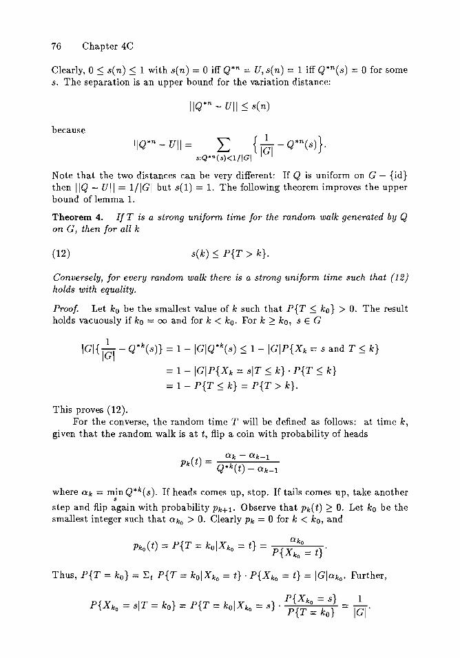
76 Chapter 4C
Clearly, 0 ~ s(n) ~ 1 with s(n) == 0 iffQ*n == U,s(n) == 1 iffQ*n(s) == 0 for somes. The separation is an upper bound for the variation distance:
IIQ*n - UII ~ s(n)
because
IIQ*n - UII = L { ~ - Q*n(s)}.s:Q ..n(s)<l/IGI I I
Note that the two distances can be very different: If Q is uniform on G - {id}then IIQ - UII = l/IGI but s(l) == 1. The following theorem improves the upperbound of lemma 1.
Theorem 4. If T is a strong uniform time for the random walk generated by Qon G, then for all k
(12) s(k) ~ P{T > k}.
Conversely, for every random walk there is a strong uniform time such that (12)holds with equality.
Proof. Let ko be the smallest value of k such thatP{T ~ ko} > o. The resultholds vacuously if ko = 00 and for k < ko. For k ~ ko, s E G
1IGI{jGT - Q*k(s)} = l-IGIQ*k(s) ~ l-IGIP{Xk = sand T ~ k}
= 1-IGIP{Xk == siT ~ k} ·P{T ~ k}= 1 - P{T ~ k} == P{T > k}.
This proves (12).For the converse, the random time T will be defined as follows: at time k,
given that the random walk is at t, flip a coin with probability of heads
where Qk = minQ*k(s). If heads comes up, stop. If tails comes up, take anothers
step and flip again with probability Pk+l. Observe that Pk( t) ~ o. Let ko be thesmallest integer such that ako > o. Clearly Pk = 0 for k < ko, and
Pko(t) = P{T = kolXko = t} = P{X::o=t}'
Thus, P{T = ko} == ~t P{T = kolXko == t} . P{Xko == t} = IGlako. Further,
P{Xko = s} 1P{Xko = siT = ko} = P{T = kolXko = s}· P{T = k
o} = jGT'
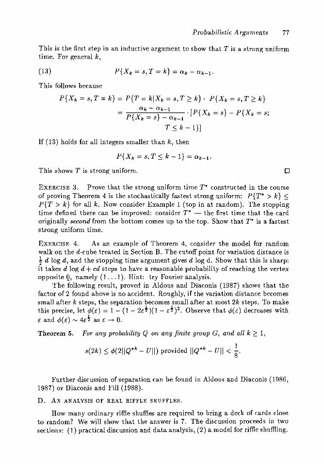
Probabilistic Arguments 77
This is the first step in an inductive argument to show that T is a strong uniformtime. For general k,
(13)
This follows because
P{Xk = s,T = k} = O'.k - O'.k-l.
P{Xk = s,T = k} = P{T = klXk = s,T ~ k}· P{Xk = s,T ~ k}O'.k - O'.k-l= P{X} · [P{Xk = s} - P{Xk = s;k = S - Qk-l
T~k-1}]
If (13) holds for all integers smaller than k, then
P{Xk = S, T ~ k - 1} = Qk-l.
This shows T is strong uniform. o
EXERCISE 3. Prove that the strong uniform time T* constructed in the courseof proving Theorem 4 is the stochastically fastest strong uniform: P{T* > k} ~
P{T> k} for all k. Now consider Example 1 (top in at random). The stoppingtime defined there can be improved: consider T* - the first time that the cardoriginally second from the bottom comes up to the top. Show that T* is a fasteststrong uniform time.
EXERCISE 4. As an example of Theorem 4, consider the model for randomwalk on the d-cube treated in Section B. The cutoff point for variation distance ist d log d, and the stopping time argument gives d log d. Show that this is sharp:it takes d log d +cd steps to have a reasonable probability of reaching the vertexopposite Q, namely (1 ... 1). Hint: try Fourier analysis.
The following result, proved in Aldous and Diaconis (1987) shows that thefactor of 2 found above is no accident. Roughly, if the variation distance becomessmall after k steps, the separation becomes small after at most 2k steps. To makethis precise, let 4>(e) = 1- (1- 2e t )(1- et )2. Observe that 4>(e) decreases withc and <jJ(e) rv 4e~ as e ~ o.Theorem 5. For any probability Q on any finite group G, and all k ~ 1,
s(2k) ~ <p(21IQ*k - UII) provided I/Q*k - UII < ~.
Further discussion of separation can be found in Aldous and Diaconis (1986,1987) or Diaconis and Fill (1988).
D. AN ANALYSIS OF REAL RIFFLE SHUFFLES.
How many ordinary riffle shuffles are required to bring a deck of cards closeto random? We will show that the answer is 7. The discussion proceeds in twosections: (1) practical discussion and data analysis, (2) a model for riffle shuffling.
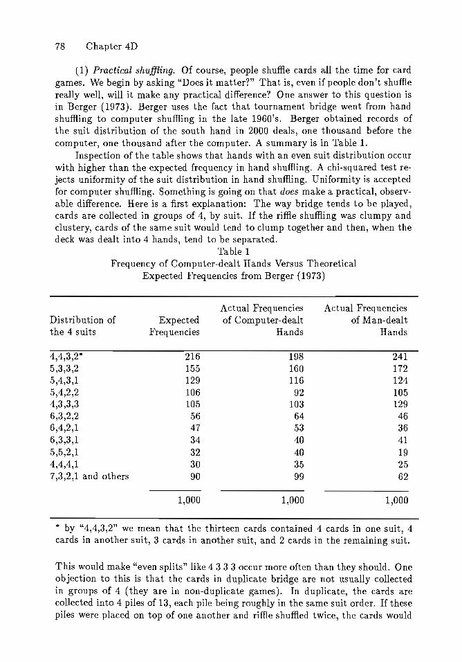
78 Chapter 4D
(1) Practical shuffling. Of course, people shuffle cards all the time for cardgames. We begin by asking "Does it matter?" That is, even if people don't shufflereally well, will it make any practical difference? One answer to this question isin Berger (1973). Berger uses the fact that tournament bridge went from handshuffling to computer shuffling in the late 1960's. Berger obtained records ofthe suit distribution of the south hand in 2000 deals, one thousand before thecomputer, one thousand after the computer. A summary is in Table 1.
Inspection of the table shows that hands with an even suit distribution occurwith higher than the expected frequency in hand shuffling. A chi-squared test rejects uniformity of the suit distribution in hand shuffling. Uniformity is acceptedfor computer shuffling. Something is going on that does make a practical, observable difference. Here is a first explanation: The way bridge tends to be played,cards are collected in groups of 4, by suit. If the riffle shuffling was clumpy andclustery, cards of the same suit would tend to clump together and then, when thedeck was dealt into 4 hands, tend to be separated.
Table 1Frequency of Computer-dealt Hands Versus Theoretical
Expected Frequencies from Berger (1973)
Actual Frequencies Actual FrequenciesDistribution of Expected of Computer-dealt of Man-dealtthe 4 suits Frequencies Hands Hands
4,4,3,2* 216 198 2415,3,3,2 155 160 1725,4,3,1 129 116 1245,4,2,2 106 92 1054,3,3,3 105 103 1296,3,2,2 56 64 466,4,2,1 47 53 366,3,3,1 34 40 415,5,2,1 32 40 194,4,4,1 30 35 257,3,2,1 and others 90 99 62
1,000 1,000 1,000
* by "4,4,3,2" we mean that the thirteen cards contained 4 cards in one suit, 4cards in another suit, 3 cards in another suit, and 2 cards in the remaining suit.
This would make "even splits" like 4 3 3 3 occur more often than they should. Oneobjection to this is that the cards in duplicate bridge are not usually collectedin groups of 4 (they are in non-duplicate games). In duplicate, the cards arecollected into 4 piles of 13, each pile being roughly in the same suit order. If thesepiles were placed on top of one another and riffle shuffled twice, the cards would
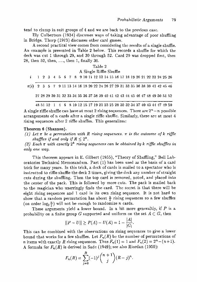
Probabilistic Arguments 79
tend to clump in suit groups of 4 and we are back to the previous case.Ely Culbertson (1934) discusses ways of taking advantage of poor shuffling
in Bridge. Thorp (1973) discusses other card games.A second practical view comes from considering the results of a single shuffle.
An example is presented in Table 2 below. This records a shuffle for which thedeck was cut 1 through 29, and 30 through 52. Card 29 was dropped first, then28, then 52, then, ..., then 1, finally 30.
Table 2A Single Riffle Shuffle
1 2 3 4 5 6 7 8 9 10 11 12 13 14 15 16 17 18 19 20 21 22 23 24 25 26
7r(i) 2 3 5 7 9 11 13 14 16 18 20 22 24 26 27 29 31 33 35 36 38 39 41 42 45 46
27 28 29 30 31 32 33 34 35 36 37 38 39 40 41 42 43 44 45 46 47 48 49 50 51 52
48 51 52 1 4 6 8 10 12 15 17 19 21 23 25 28 30 32 34 37 40 43 44 47 49 50
A single riffle shuffle can have at most 2 rising sequences. There are 2n - n possiblearrangements of n cards after a single riffle shuffle. Similarly, there are at most 4rising sequences after 2 riffle shuffles. This generalizes:
Theorem 6 (Shannon).(1) Let 1r be a permutation with R rising sequences. 1r is the outcome of k riffle
shuffles if and only if R ~ 2k •
(2) Each 1r with exactly 2k rising sequences can be obtained by k riffle shuffles inonly one way.
This theorem appears in E. Gilbert (1955), "Theory of Shuffling," Bell Laboratories Technical Memorandum. Part (1) has been used as the basis of a cardtrick for many years. In this trick, a deck of cards is mailed to a spectator who isinstructed to riffle shuffle the deck 3 times, giving the deck any number of straightcuts during the shuffling. Then the top card is removed, noted, and placed intothe center of the pack. This is followed by more cuts. The pack is mailed backto the magician who unerringly finds the card. The secret is that there will beeight rising sequences and 1 card in its own rising sequence. It is not hard toshow that a random permutation has about ~ rising sequences so a few shuffles(on order log2 ¥-) will not be enough to randomize n cards.
These arguments yield a lower bound. In a bit more generaltiy, if P is aprobability on a finite group G supported and uniform on the set A c G, then
liP - UII ~ P(A) - U(A) = 1 - :~\.This can be combined with the observations on rising sequences to give a lowerbound that works for a few shuffles. Let Fn(R) be the number of permutations ofn items with exactly R rising sequences. Thus Fn (l) = 1 and Fn (2) = 2n -(n+1).A formula for Fn(R) is derived in Sade (1949); see also Riordan (1950):
Fn(R) = "£(-1)i (n ~ 1) (R _ j)n.. 0 JJ=
80 Chapter 4D
In k shuffles, the total number of permutations that can be achieved is Tn(k) =2k
2: Fn(R). Thus 1 - Tn(k)jn! is a lower bound for the variation distance. ForR=In = 52, the lower bound is larger than .99 for 1 ~ k ~ 4. For k = 5 it is .38, fork = 6 it is zero.
Observe that this approach makes no assumptions about the stochastic mechanism for shuffling, but the argument breaks down at 6 shuffles.(2) A probability model. The following model for riffle shuffling was suggested by
Shannon and Gilbert, and Reeds.
1st description: Cut the n card deck according to a binomial distribution withparameters t, n. Suppose k cards are cut off. Pick one of the (k') possible riffleshuffles uniformly.
2nd description: Cut the n card deck according to a binomial distribution withparameters t, n. Suppose k cards are cut off and held in the left hand and n - kheld in the right hand. Drop cards with probability proportional to packet size.Thus the chance that a card is dropped first from the left hand is ~. If thishappens, the chance that the left hand drops a second card is ~=~; and so on.
3rd description: To generate the inverse shuffle, label the back of each card withthe result of an independent fair coin flip: {O, I}. Remove all cards labeled 0 andplace them on top of the deck, keeping the cards otherwise in the same relativeorder.
LEMMA 2. The three descriptions yield the same probability distribution.
Proof. The 1st and 3rd descriptions are equivalent: indeed, the binary labelingchooses a binomial number of zeros and conditional on this choice, all possibleplacements of the zeros are equally likely. The 1st and 2nd descriptions are equivalent: Suppose k cards have been cut off. Under the 2nd description, the chanceof a shuffle is the chance of the sequence of drops D I , D 2 , ••• , D n , where each Dican be L or Rand k Di's must be Land n - k Di's must be R. The chance ofany such sequence is k!(n - k)!/nL 0
Remarks. This shuffling mechanism has some claim to being the "most random"subject to the binomial cutting. It has the largest entropy, for example. As amodel for shuffling, it yields shuffles a bit "clumpier" than either the shufflesof Diaconis or Reeds discussed in remark (e) below. Only half the packets areexpected to be of size 1, a quarter of size 2, etc. Of course, extremely neat shufflesare not necessarily good for randomization. A perfect shuffle is completely nonrandom for example, eight perfect shuffles bring the deck back to order. SeeDiaconis, Graham, and Kantor (1983). Mellish (1973) discusses these issues.
To proceed further, we construct a strong uniform time for this model ofshuffling. To begin, observe that the variation distance is invariant under 1-1transformations, so it is the same problem to bound the number of inverse shufflesrequired to get close to random.
The results of repeated inverse shuffles of n cards can be recorded by forming
Probabilistic Arguments 81
a binary matrix with n rows. The first column records the zeros and ones thatdetermine the first shuffle, and so on. The ith row of the matrix is associated tothe ith card in the original ordering of the deck, recording in coordinate j thebehavior of this card on the jth shuffle.
LEMMA 3 (Reeds). Let T be the first time that the binary matrix formed frominverse shuffling has distinct rows. Then T is a strong uniform time.
Proof. The matrix can be considered as formed by flipping a fair coin to fillout the i, j entry. At every stage, the rows are independent binary vectors. Thejoint distribution of the rows, conditional on being all distinct, is invariant underpermutations.
After the first inverse shuffle, all cards associated to binary vectors startingwith 0 are above cards with binary vectors starting with 1. After two shuffles,cards associated with binary vectors starting (0,0) are on top followed by cardsassociated to vectors beginning (1,0), followed by (0,1), followed by (1,1) at thebottom of the deck.
Inductively, the inverse shuffles sort the binary vectors starting with 0 areabove cards with binary vectors starting with 1. After two shuffles, cards associated with binary vectors starting (0,0) are on top followed by cards associated tovectors beginning (1,0), followed by (0,1), followed by (1,1) at the bottom of thedeck.
Inductively, the inverse shuffles sort the binary vectors (from right to left)in lexographic order. At time T the vectors are all distinct, and all sorted. Bypermutation invariance, any of the n cards is equally likely to have been associatedwith the smallest row of the matrix (and so be on top). Similarly, at time T, alln! orders are equally likely. 0
To complete this analysis, the chance that T > k must be computed. Thisis simply the probability that if n balls are dropped into 2k boxes there are nottwo or more balls in a box. If the balls are thought of as people, and the boxesas birthdays, we have the familiar question of the birthday problem and its wellknown answer. This yields:
Theorem 7. For Q the Gilbert-Shannon-Reeds distribution defined in Lemma 2,
n-l .
(14) IIQ*k - UII ~ P{T > k} = 1- IT(1- 2~k)'i=l
Standard calculus shows that if k = 2log2(nfc),
n ~ c c2P{T> k} "-J 1 - e- 2 "-J-.
00 0 2
In this sense, 2 log n is the cut off point for this bound. Exact computation ofthe right side of (14) when n = 52 gives the bounds
82 Chapter 4D
k upper bound10 .7311 .4812 .2813 .1514 .08
Remark (a). The lovely new idea here is to consider shuffling as inverse sorting.The argument works for any symmetric method of labelling the cards. For example, biased cuts can be modeled by flipping an unfair coin. To model cuttingoff exactly j cards each time, fill the columns of the matrix with the results of ndraws without replacement from an urn containing j balls labelled zero and n - jballs labelled one. The first time all vectors are different is a strong uniform time.These lead to slightly unorthodox birthday problems which turn out to be easyto work with.
Observe that the shuffle in which only 1 card is cut off and randomly riffledinto the deck is the "top in at random" shuffle of example 1. The two stoppingtimes are the same!
Remark (b). The argument can be refined. Suppose shuffling is stopped slightlybefore all rows of the matrix are distinct - e.g., stop after 2 log n shuffles. Cardsassociated to identical binary rows correspond to cards in their original relativepositions. It is possible to bound how far such permutations are from uniformand get bounds on llQ*k - Ull. Reeds (1981) has used such arguments to showthat 9 or fewer shuffles make the variation distance small for 52 cards.
Remark (e). A variety of ad hoc techniques have been used to get lower bounds.One simple method that works well is simply to follow the top card after repeatedshuffles. This executes a Markov chain on n states with a simple transition matrix.For n in the range of real deck sizes, n X n matrices can be numerically multipliedand then the variation distance to uniform computed. Reeds (1981) has carriedthis out for decks of size 52 and shown that IIQ*6 - UII ~ .1. Techniques whichallow asymptotic verification that k = 3/2 log2 n is the right cutoff for large n aredescribed in Aldous (1983). These analyses and the results quoted above suggestthat seven riffle shuffles are needed to get close to random.
Remark (d). Other mathematical models for riffle shuffling are suggested in Donner and Uppuluri (1970), Epstein (1977), and Thorp (1973). Borel and Cheron(1955) and Kosambi and Rao (1958) discuss the problem in a less formal way.Where conclusions are drawn, 6 to 7 shuffles are recommended to randomize 52cards.
Remark (e) some data analysis. Of course, our ability to shuffle cards depends onpractice and agility. The model produces shuffles with single cards being droppedabout 1/2 of the time, pairs of cards being dropped about 1/4 of the time, and icard blocks being dropped about 1/2i of the time.
To get a feeling for the difference between shufflers, the following experimentwas performed: Diaconis and Reeds each shuffled a deck of 52 cards about 100
Probabilistic Arguments 83
times; every permutation was recorded. The following summary statistics arerelevant.
Diaconis - 103 Shuffles# cut off top 23 24 25 26 27 28 29
2 4 22 32 33 9 1
In shuffling, the left hand dropped first 44 times. In all there were 4,376 "packets"dropped. The counts and proportions were
1 2 3 4 53501 793 63 15 4
.80 .18 .01 .00 .00
The packet size distribution of first dropped packets was1 234 5
.37 .37 .17 .1 .01
Reeds - 100 Shuffles# cut off top 23 24 25 26 27 28 29 30 31
2 2 8 16 23 26 16 5 2
In shuffling, the left hand dropped first 18 times. In all there were 3,375 "packets"dropped. The counts and proportions were
1 2 3 4 5 6 7 8 9 10 11 12 132102 931 228 68 24 12 3 3 2 0 0 1 1
.62 .28 .07 .02 .01 .00 .00 .00 .00 .00 .00 .00 .00
Diaconis does very neat shuffles and can be compared to aLas Vegas dealer. Reedsshuffles like an "ordinary person." Observe that the first drops for Diaconis arequite different from the average drop. Even though the two types of shuffiers arefairly different, to a first approximation they are quite similar, both dropping 1,2, or 3 cards most of the time.
Remark (I). There is another equivalent way to describe repeated riffle shufflesunder the Gilbert-Shannon-Reeds model that suggests much further research. Thefollowing evolved in conversations with Izzy Katzp.elson and Jim Reeds. Beginby dropping n points at random into the unit interval and labeling them, left toright, as 1,2, ... , n. The transformation T(x) = 2x(mod 1) (sometimes called theBaker's transformation) maps the unit interval into itself and so permutes thepoints. T takes each of the two half intervals and stretches it out to cover [0, 1].There are a binomial number of points in each half and T shuffles them together.Arguing as in Lemma 1 above, it is easy to see that the induced permutation isprecisely a basic riffle shuffle. Further, successive shuffles are independent (theydepend on successive bits of the underlying uniform variables).
To complete the argument, consider k chosen so large that n points droppedat random into [0, 1] fall into disjoint pieces of a partition with pieces of length1/2k , with high probability. Picture a point in a piece of the partition. After kshuffles, the piece is stretched out to cover [0, 1]. The point is randomly distributedin the piece of the partition. After k shuffles it's randomly distributed in [0,1].Further, points in disjoint pieces are independent. After k shuffles, the n pointsare in random relative arrangement (given that they fall into disjoint pieces).
84 Chapter 4E
This argument generalizes to some extent (x ---+ kjx(mod 1) on shuffle j forinteger kj ). It should be possible to take other measure preserving transformations(toral endomorphisms of the unit square (see WaIters (1982)) and convert themto other shuffles.
E. COUPLING.
There is a more widely known purely probabilistic argument called coupling.Again, perhaps it is best to begin with an example, this one is due to DavidAldous.
Example l-Borel's shuffle. Borel and Cheron (1955) discuss several methodsof mixing up cards. They give the following as an open problem: begin with ncards. Take the top card off and put it into the deck at a random position. Takethe bottom card off and put it into the deck at a random position. Continuealternately placing top in at random, bottom in at random.
Observe that there is no longer an obvious stopping time. The followingelegant coupling argument has been suggested by David Aldous. It is better towork with the inverse shuffle that removes a random card and places it alternatelyon top or bottom. Because of the invariance of variation distance under 1-1 maps(IIQ - UII = IIQh-1 - Uh-111 for any 1-1 function G ---+ G) the two shuffles havethe same rates of convergence (see exercise 3 of Chapter 3).
To describe a "coupling", consider a second deck of cards. The first deckstarts in order {I, 2, 3, ... , n}. The second deck starts in a random order. Acard is determined at each stage by shuffling a third deck and choosing a card atrandom. Say the first card chosen is the six of hearts. Remove the six from deck1 and place it on top. Remove the six from deck two and place it on top. Notethat from each deck's marginal vantage point, a card was removed at random andplaced on top.
The second step is to reshuffle the 3rd deck and choose a second card, say theAce of spades. This is removed and placed at the bottom of each deck. Continuein this way, each time choosing a card at random from the third deck, removingthe card from decks one and two, and placing the card alternately on top andbottom.
As this process continues, decks one and two match up. The same cardsbeing in the same order at top and bottom. If the same card is chosen again,the procedure keeps the same number of matches. A new match is created foreach new card touched. Let T be the first time that each card has been touched.Clearly, the two decks are in the same order, but deck two started at random, andso remains random. It follows that deck one is random at time T. The bound onthe coupon collector's problem yields
Theorem 8. For Borel's shuffle, if k = n log n + en for e > 0,

Probabilistic Arguments 85
EXERCISE 5. Find a strong uniform time to get a bound in Borel's problem.To discuss coupling more carefully, we need the following fact about variation
distance:
LEMMA 4. Let S be a finite set. Let PI and P2 be probability measures on S.Let Q be a probability on S X S with margins PI and P2 • Let ~ be the diagonal:~ = {(s,s):s E S} then,
Proof.
IPI(A) - P2(A)1 == IQ(A X S) - Q(S X A)I== IQ(A X Sn~) +Q(A X S n ~C) - Q(S X A n~)
- Q(S X A n ~C)I.
The first and third numbers in the absolute value sign are equal. The secondand fourth give a difference between two numbers, both non-negative and smallerthan Q(LlC). D
Remarks. The inequality is sharp in the sense that there is a Q wh~ch achievesequality. A proof and discussion may be found in V. Strassen (1965). This Qallows the following interpretation of variation distance: II PI - P211 = e if and onlyif there are two random variables, Xl distributed as PI and X 2 distributed as P2,such that Xl = X 2 with probability 1 - e; Xl and X 2 may be arbitrarily differentwith probability E. Another interpretation: the optimal Q is most concentratedabout the diagonal with these fixed margins.
Let us define a coupling for a Markov chain on state space I, with transitionprobability Pi(j), and stationary distribution '!r. We will work with Markoviancouplings. These are processes on I X I with transition probability Q satisfying
L Qi,j(S, t) = Pi(s) for all jt
L Qi,j(S, t) = Pj(t) for all i.s
These conditions just say that the transition mechanism of each component ofthe vector process is Pi(j). Call the vector process (Xf, X~). Suppose that Xlstarts in i and X 2 starts according to '!r. Let T == min{k: X~ == X~}. This T is astopping time. Suppose that T is finite with probability 1. Let
x 3 _ {X~ k~ Tk - Xf k > T.
The process (Xk, X2) is called a coupling, the interpretation being that the twoprocesses evolve until they are equal, at which time they couple, and thereafter
86 Chapter 4E
remain equal. The usefulness of coupling depends on being able to get our handson T: Let pik be the law of the process after k steps started from i.
LEMMA 5. (Coupling inequality). Ilpik
- 11"11 ~ peT > k).
Proof. Take Q to be the distribution of (X~, XZ). This Q has marginaldistributions Pike ) and 11". Lemma 4 implies that
o
Remarks. It is instructive to note that while the distribution of XT is stationary(and so uniform in our examples) the time T is not a strong uniform time as wehave defined it; for this requires P(Xk E AIT = k) = U(A) for all k.
Remarks. Example 1 gives an actual construction of Qij(kf). It might beinstructive to write down what Qij(kf) is for this example. Griffeath (1975),Pitman (1976) or Goldstein (1979) show that the argument is tight in the sensethat there is a coupling that achieves the total variation distance. This couplingcannot be taken as Markovian in general (that is, the bivariate process needn'tbe Markov).
Example 2. Random walk on the d-cube. Here G = zt. Take
P(Q) = p, P(1 0 ... 0) = P(O 1 00 ... 0) ... = P(O .. . 1) = (1- p)/d.
Here is a coupling argument, due to David Aldous, for bounding convergenceto uniform. Consider two cubes. The process XJ starts at zero, XJ starts ina uniformly distributed position. The pair (Xl, Xl) evolves as follows: if Xland xl differ in an odd number of places, the two processes take independentsteps according to P. If Xl and Xl differ in an even number of places, thenwith probability p each remains unchanged. If they don't stay the same, thenpick an index j at random in {I, 2, ... , d}. If the jth component of Xl and Xlagree, change that component to its opposite (mod 2) in both processes. If the jthcomponent of xl and Xl do not agree, complement the jth component of Xl andthe next non-agreeing component of xl from j counting cyclically. This forcesxl and xl to agree in two more coordinates. Once the number of disagreeingplaces is even, it stays even, so the coupled process "gets together" very rapidly.Of course, once Xl = Xl, they stay coupled.
EXERCISE 6. Analyze the coupling time T and get a bound on the rate ofconvergence for Example 2. Compare this with the right rate derived fromFourier analysis.
Matthews (1986b) has constructed non-Markovian couplings that give theright rate of convergence for the cube.
Coupling is a very widely used tool which has many success stories to itscredit. Aldous (1983a) gives a number of card shuffling examples. Robin Pemantle
Probabilistic Arguments 87
(1989) has given a marvelous coupling analysis of the familiar over-hand shuffle.For a range of reasonable models he shows that order n 2 shuffles are required tomix up n cards. Thus about 2,500 shuffles are required for 52 cards. This shouldbe compared with 7 or 8 riffle shuffles, and the computation that a single riffleand single over-hand shuffle produce the same number of distinct permutations.
Aldous and Diaconis (1987a) and Thorisson (1987) study the relation betweencoupling and strong uniform times. Briefly, for any strong uniform time there isa coupling with the same time. Thus couplings can occur faster in principle.
Theorem 5 of Section C shows that couplings can only speed things up by afactor of at most 2. The example of simple random walk on the cube shows thatthis actually happens: it takes t n log n +cn steps to make the variation distancesmall; t n log n +cn steps are needed to make the separation small.
Despite the similarities, the connection is fairly formal. The way of thinking,and basic examples, can be very different. There is no known direct couplingargument to get anything better than n 2 for random transpositions, while stronguniform times or Fourier analysis show the right rate is order n log n. Similarly,there is no strong uniform time for the over-hand shuffle, or the shuffle that picksa card at random and switches it with a neighbor. Coupling can handle theseproblems.
F. FIRST HITS AND FIRST TIME TO COVER ALL.
(1) Introduction. Most of the work in this and the previous chapter has beendevoted to estimating rates of convergence to uniformity. There are manyother natural questions connectd to random walk. One may ask• How long does it take to hit a fixed state (or set of states) from a given (orrandom) start?• How long does it take to hit every state?• How long until the first return to the starting state? How far away is thewalk likely to get before first returning? flow many states does the walk hitbefore first returning? What is the maximum number of times any state hasbeen visited at first return?• How long does a walk take before it hits a point previously hit (the birthdayproblem for random walk)?David Aldous has introduced an important heuristic which suggests and ex
plains answers to such questions, and sometimes allows a proof using only boundson convergence to stationarity.
The idea is as follows. Suppose a specific random walk on a group G israpidly mixing in the sense that the variation distance is less than t after k stepswith log k of order a polynomial in logJGI. Then, the random walk forgets whereit is rapidly, and successive steps may be thought about as the position of balls,dropped at random, into JGI boxes.
Questions about balls in boxes are well understood. For example, the meanwaiting time T until a ball is dropped into a fixed box is IGI and
TP{ iGT > t} -+ e-t as G -+ 00.
88 Chapter 4F
This suggests that a rapidly mixing random walk takes about ICI steps to hit afixed point and the waiting time is approximately exponential. A precise versionis given in (2) below.
As a second example, the waiting time V for all boxes to have at least one ballis well studied as the coupon collector's problem. For balls dropped at randominto ICI boxes, it takes about IClloglCI balls to have a good chance of filling allboxes. Results in Feller (1968, pg. 106) yield
P{ V - IClloglGI < } --t -e-~ IGI --tIGI - x e as 00.
This suggests that a rapidly mixing random walk takes about IG)logIG) steps tocover all points. (3) below gives some precise results due to Aldous and Matthews.
Section 4 points to what little is known about other problems on the listabove.
(2) First hit distributions. The heuristics above are right "up to constants."One remarkable finding of Aldous (1982, 1983b) is that only one other feature ofthe walk enters. This is a measure of the amount of time the walk spends in itsstarting state in a short time period. Consider throughout a random walk on afinite group G. The transition mechanism is assumed to be aperiodic, and theuniform distribution on G is the stationary distribution.
Standard renewal theory implies that R(s; t), the amount of time the walkspends in a fixed state s up to time t, is asymptotically tlICI. Moreover
R = lim E{R(s; t)} - tllGIt-+oo
exists and is finite. By homogeneity R doesn't depend on s. Aldous (1983b)argues that for rapidly mixing walks, R can be interpreted as the mean numberof visits the random walk spends in its initial state in a short time. For most ofthe examples in this and the previous chapter, R = 1.
With this notation, some careful results can be stated.
Theorem 9. (Aldous). Let Ts be the first time a random walk starting in auniformly chosen position hits state s. Then
(1) E(Ts ) = RIGI for all s E G.
Let T = i~f{\lp*k - U\\ ~ 1/2e}. Then
(2) sup IP{Ts > t} - e-t/RIGII ~ 1f'(T IRIGI),t~O
with "p( x) tending monotonically to zero as x tends to O.
Remarks. Part (2) makes precise the heuristics of the previous section. Considera process like simple random walk on the d-cube. Then IGI = 2d , and T ==td log d, R = 1, and (1) and (2) recapture the limiting results derived in Chapter
Probabilistic Arguments 89
3R. Aldous (1983b) gives similar results for the first hitting time to arbitrary setswith any starting distribution.
Most random walks considered above have T /IGI ---* o. An exception is simplerandom walk on Zn, where T is of order n2 • The wait to first hit a point has arather complicated distribution (see Chapter 3R). Flatto, Odlyzko, and Wales(1985) use Fourier analytic methods to get higher order correction terms.
(3) Time to cover all. Let G be a finite group and P a probability withconvolutions that converge to uniform aperiodically. Let V be the first time thata random walk hits every point in G. Note that the distribution of V doesn'tdepend on the starting state. Let T and R be as defined in Section 2. Aldous(1983a) proves
Theorem 10.V ( log( 1 + T))
El RIGlloglGI - 11 ~ 7/J loglGI
with 1jJ(x) tending monotonically to zero as x tends to o.
Remark. In the case of the cube, log(1 + T) f'V log d, loglCI f'V d log 2, so theratio tends to zero. Analogs of the extreme value limits for the coupon collector'sproblem are not established in this generality. However, Matthews (1985) hasestablished limit theorems for many of the examples where Fourier analysis canbe successfully applied.
Usually the results follow the heuristic. For the cube there is an extra factorof 2. Matthews shows
for all fixed x as n tends to infinity. Here R f'V 1 + ~ which explains the 2.Matthews' argument works by getting upper and lower bounds on the re
quired probability. These apply to problems like first time for a Markov chainto hit every point in a finite state space or first time for Brownian motion tocome within £ of every point on a high-dimensional sphere. The bounds merge asIGI ~ 00 for random walk problems.
(4) Other problems. There has been some work on special cases of the problems listed in (1) above. Aldous (1985) started to classify the kind of limitingbehavior that can occur in the birthday problem for random walk. Diaconis andSmith (1988) have begun to develop a fluctuation theory (as in Chapter 3 of Feller(1968)). Some neat results emerge for nearest neighbor random walk on a 2-pointhomogeneous space. For example, on the n-cube, the probability that randomwalk starting at (00 ... 0) hits a given point at any specified distance less than nbefore returning to zero tends to 1 as n tends to 00. The probability tends to 1/2for (1, ... ,1).
This seems like a rich collection of reasonably tractable problems. Passingto the limit should give results for the approximating diffusions (e.g., OrnsteinUhlenbeck process for the cube) in much the same way as results about simplerandom walk lead to results for Brownian lTIotion.
90 Chapter 4G
G. SOME OPEN PROBLEMS ON RANDOM WALK AND STRONG UNIFORM TIMES.
Here is a small list of problems that seem worth careful work.(1) The slowest shuffle. Arunas Rudvalis has suggested the following can
didate for the slowest shuffle: At each time, the top card is placed either atthe bottom, or second from the bottom, each with chance t. How long does ittake to get random? Is this the slowest shuffle equally supported at 2 generatingpermutations?
(2) Let G == Zn. Pick k points in G, and repeatedly choose one of them atrandom. This determines a random walk. What are the slowest k points (givenno paritiy problems) - a "arc" near zero? (i.e. the set of points j with Ijl < k/2.)What are the fastest k points? Andy Greenhalgh has shown how to get rate n1 /
k
by an appropriate choice. What's the rate for "most" sets of k points? Thesequestions are already non-trivial for k = 3. They are also worth studying when kgrows with n.
(3) Moving on to other groups, Aldous and Diaconis showed that for mostmeasures P on a finite group G, IIP*P- U/I ~ Ibl' so for G large, most measuresare random after two steps. To get an interesting theory, constraints must be puton the support. Andre Broder asked the following: pick a pair of elements in Sn'Consider the walk generated by choosing both of these elements at random. It canbe shown that such a pair generates Sn with probability 3/4 asymptotically. Isthe walk random after a polynomial number of steps? Similar problems are worthinvestigating for any of the classical infinite families of finite simple groups (I'dtry PGLn(q)). Back on Sn; it seems that any "reasonable" shuffle gets randomin at most a polynomial number of steps.
(4) The 15 puzzle. This familiar puzzle has 15 blocks arranged in a 4 X 4grid. At each state, any of the blocks can be slid into the blank. Suppose uniformchoices are made among the current possibilities.
Here is a simplified version: Consider the blank as a 16th block, and considerthe puzzle on a "torus." An allowable move now involves picking one of the 16squares at random, and then a direction (North, South, East, West) and "cycling"that square in the chosen direction. For example, the bottom row might changefrom 13, 14, 15, 16 to 16, 13, 14, 15 or to 14, 15, 16, 13. It is not hard to showthat it takes order n3 steps to randomize a single square (on an n X n grid). Ipresume that order n 3 log n steps suffice to randomize everything. For a 4 X 4, thisgives about 90 "moves" to randomize. I presume this simplified version convergesto uniform faster than the original 15 puzzle. Similar questions can be asked forother puzzles such as Rubic's cube.
(5) The affine group. Consider random walks of form X n = anXn- 1 +bn(mod p). Here p is a fixed number (perhaps a prime) and (an,bn) are chosen at random: e.g., an = 2 or t(mod p), bn = ±1. It seems that the right answerfor these is (log p)a for a = 1 or 2. The best that has been proved at present isorder p2 (see Diaconis and Shahshahani (1986a).
(6) Thorp's shuffle. A simple model for a random riffle shuffle has beendescribed by Thorp (1973). Cut the deck exactly in half. Start to drop the cardsfrom left or right hand as with an ordinary shuffle. At each time, choose left or
Probabilistic Arguments 91
right with chance t. Whatever is chosen, drop that card, and then a card fromthe opposite half. Continue inductively. I think use of the mathematics of shufflenets (or work on sorting in parallel) will allow an elegant solution to this problem.
(7) Continuous groups. We have no examples of a strong uniform time argument being used to get rates of convergence for a random walk on a compact,infinite group. It may be necessary to change the distance to the Prohorov metric.For problems like random reflections (see Diaconis and Shahshahani (1968a)) orrandom walk on the circle determined by repeatedly choosing a point in a smallarc uniformly, there is convergence in total variation metric.
(8) The cutoff phenomenon. The most striking finding is the existence ofsharp phase transition, IIp*k - UII cutting down from 1 to zero in a relativelyshort time. It would be great to understand if this usually happens. As explainedin problem (3) above, restrictions will have to be put on the support.
(9) Relations between various approaches. A curious feature of the examplesis that usually if one method of attack works (e. g., Fourier analysis, or coupling,or strong uniform times), then all the methods work. There must be a reason.The greatest mystery is to understand the connections between the analytic andprobabilistic methods. One place to start is "top in at random," the first exampleof Chapter 4. This can be done by strong uniform times and coupling. Theremust be a way to do it Fourier analytically.
Chapter 5. Examples of Data on Permutations andHomogeneous Spaces
To fix ideas, as well as to make contact with reality, it is useful to have acollection of real data sets on hand.
A. PERMUTATION DATA.
(1) Large sets of rankings are sometimes generated in psychophysical experiments(rank these sounds for loudness), taste testing experiments (rank these 5types of coffee ice cream), or surveys. To give an example, in 1972, theNational Opinion Research Center included the following question in one oftheir surveys: Where do you want to live? Rank the following 3 options: ina big city; near a big city (~ 50 miles); far from a big city (> 50 miles). Thedata from 1439 respondents was
city suburbs country #1 2 3 2421 3 2 282 1 3 1703 1 2 6282 3 1 123 2 1 359
Let us briefly discuss this data. The modal rank is 1i ~ - people preferthe suburbs, then country, then city. This is born out by simple averages: 270people ranked city first, 798 ranked suburb first, 371 ranked country first.
The 2 small counts lead to an interesting interpretation. Both violate theunfolding hypothesis of Coombs (1964). To spell this out a bit, suppose people'srankings are chosen in accordance with the ideal distance from the city, differentpeople having different preferences. Thus, one chooses the rank one location andthen "unfolds" around it. In this model (I 5 ~) is impossible since if one mostprefers being in the city, one must prefer being close to the city to being far away.The number of permutations of the set 1,2, ... , n consistent with unfolding isabout 2n
- 1 , so many arrangements are ruled out. Unfolding is a nice idea, butdistance to the city might not determine things for someone who works in the suburbs and doesn't want to live where they work. If you ask people to rank ordertemperature for tea (hot, medium, cold), you don't expect the unfolding restriction to hold, but if you ask people to rank order sugar teaspoons (0, t, 1, ~, 2)you do expect the data to be consistent with unfolding.
Further analysis of the distance to cities data is in Chapter 8. Duncan andBrody (1982) discuss these data in some detail.
92
Examples of Data on Permutations and Homogeneous Spaces 93
Ranked data often comes with other variables - rankings for men andwomen, or by income being examples. In the data on distance to cities, theactual dwelling place of the respondent is available. Methods for dealing withcovariates are developed in Chapter 9.
It is worth pointing to a common problem not represented in the cities data.Because n! grows so rapidly, one can have a fairly large data set of rankings andstill only have a small proportion of the possible orders represented. For example,I am considering a data set in which 129 black students and 98 white studentswere asked to rank "score, instrument, solo, benediction, suite" from the leastrelated to "song" to the most strongly related to "song." Here, there cannotbe very many repeats in each ranking. In another data set, quoted in Feigin andCohen (1978), 148 people ranked 10 occupations for desirability. Clearly, the ratioof the sample size to n! has a limiting effect on what kind of models can be fit tothe data.(2) Pairs of permutations often arise as in "rank order the class on the midterm
and final." Similarly, small sets of rankings arise as in a panel of judges ranking a set of contestants. A large collection of examples appears in Chapter7A.
(3) The Draft Lottery. In 1970, a single "random" permutation in S365 waschosen. This permutation was used to fix the order of induction into thearmy. The actual permutation is shown in Table 1. For discussion of thisdata set, see the article by S. E. Fienberg (1971).As Fienberg reports, it was widely claimed that the permutation tended to
have lower order months Jan., Feb., ... having higher numbers. The Spearmanrank correlation coefficient is -.226, significant at the .001 level. Figure 2, basedon Figure 1, shows the average lottery number by month. The evidence seemsstrong until we reflect on the problems of pattern finding in a single data sourceafter agressive data analysis.
Further analysis of this data is given in example 1 of Chapter 7A.
B. PARTIALLY RANKED DATA.
There are numerous examples in which people rank a long list only partially.For example, people might be asked to rank their favorite 10 out of 40 movies,a typical ranking yielding (a1' a2, ... , a10) with a1 the name of the movie rankedfirst, etc. Alternatively people might be asked to choose a committee of 10 out of40, not ranking within. Then a typical selection yields the set {at, a2, ... , a10}.
In each case the symmetric group S40 acts transitively on the partial rankingswhich may thus be represented as homogeneous spaces for S40 (see Chapter 3-Ffor definitions). For ranked 10 out of 40 the homogeneous space is S40/ S30. Forunranked 10 out of 40, the homogeneous space is S40/ S10 x S30.
Here are some real examples of such data.Example 1. American Psychological Association data. The American Psychological Association is a large professional group (about 50,000 members). To vote fora president, members rank order five candidates. A winner is chosen by the Haresystem: Look at the first place votes for all five candidates. If there is no majoritycandidate (~ 50%) delete the candidate with the fewest first place votes. Ballots
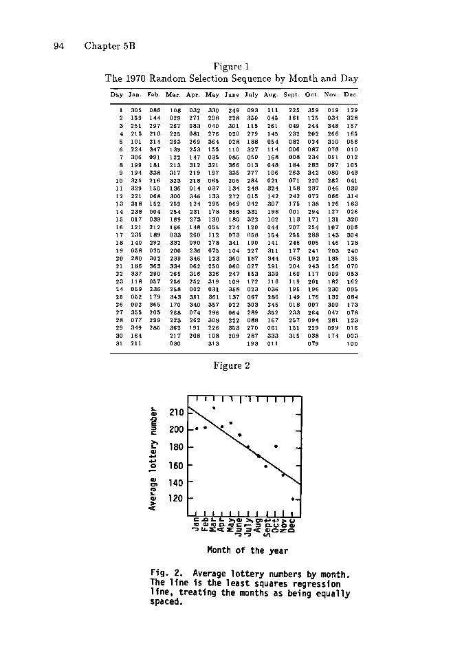
94 Chapter 5B
Figure 1The 1970 Random Selection Sequence by Month and Day
Day Jan. Feb. Mar. Apr. May June July Aug. Sept. Oct. Nov. Dec.
1 305 086 108 032 330 249 093 111 225 359 019 1292 159 144 029 271 298 228 350 045 161 125 034 3283 251 297 267 083 040 301 115 261 049 244 348 1574 215 210 225 081 276 020 279 145 232 202 266 1655 101 214 293 269 364 028 188 054 082 024 310 0566 224 347 139 253 155 110 327 114 006 087 076 0107 306 091 122 147 035 085 050 168 008 234 051 0128 199 181 213 312 321 366 013 048 184 283 097 1059 194 338 317 219 197 335 277 106 263 342 080 043
10 325 216 323 218 065 206 284 021 071 220 282 04111 329 150 136 014 037 134 248 324 158 237 046 03912 221 068 300 346 133 272 015 142 242 072 066 31413 318 152 259 124 295 069 042 307 175 138 126 16314 238 004 254 231 178 356 331 198 001 294 127 02615 017 039 169 273 130 180 322 102 113 171 131 32016 121 212 166 148 055 274 120 044 207 254 107 09617 235 189 033 260 112 073 058 154 255 288 143 30418 140 292 332 090 278 341 190 141 246 005 146 12819 058 025 200 236 075 104 227 311 177 241 203 24020 280 302 239 346 123 360 187 344 063 192 185 13521 186 363 334 062 250 060 027 291 204 243 156 07022 337 290 265 316 326 247 153 339 160 117 009 05323 118 057 256 252 319 109 172 116 119 201 182 16224 059 236 258 002 031 358 023 036 195 196 230 09525 052 179 343 351 361 137 067 286 149 176 132 08426 092 365 170 340 357 022 303 245 018 007 309 17327 355 205 268 074 296 064 289 352 233 264 047 07828 077 299 223 262 308 222 088 167 257 094 281 12329 349 285 362 191 226 353 270 061 151 229 099 01630 164 217 208 108 209 287 333 315 038 174 00331 211 030 313 193 011 079 100
Figure 2
s.. 210cu.cE
200::tc:
~ 180cu+'...,
1600r-
eil 140en
"'...120cu
><
Month of the year
Fig. 2. Average lottery numbers by month.The line is the least squares regress;online, treating the months as being equallyspaced.
Examples of Data on Permutations and Homogeneous Spaces 95
with this candidate are relabelled to have the remaining candidates in the samerelative order. The procedure is now continued with the four remaining candidates. Fishburn (1973), Doran (1979), or Brams and Fishburn (1983) discuss thesystem and relevant literature.
A considerable number of voters do not rank all five candidates. For example,in the year being considered the number of voters ranking q of the candidates was
q #123
5
5141 }2462 97112108
5738
15,449
Thus there were 5,738 complete rankings, but 5,141 only voted for their firstchoice. In all, more than half of the ballots were incomplete. It is assumed thatpeople who rank 4 candidates meant to rank the 5th candidate last.
It is natural to inquire whether the partially ranked ballots are different fromthe restriction of the complete ballots (or vary with q). Such considerations shouldplay a role in deciding on a final voting rule, and on deciding on ballot design andelection publicity in following years.
Table 1 gives the complete data. The data are arranged as (rank, #) whererank is a five-digit number, whose ith digit represents the rank given to candidatei (a zero or blank means that this is a partial ranking, in which candidate i has notbeen ranked). For example, the first entry (1, 1022) indicates that candidate 5 wasranked first by 1022 people who didn't rank anyone else. The second entry (10,1145) indicates that candidate 4 was ranked first by 1145 people (who didn't rankanyone else). The first 5 entries give the totals for singly ranked items. The next20 entries give totals for people ranking 2 of the 5 candidates. For example 143people ranked candidate 5 first and candidate 4 second (and didn't rank anyoneelse). These data are analyzed by Diaconis (1989).
Example 2. k sets of an n set. If people are asked to choose their favorite k of n,without ranking within (as in choosing a committee or set of invitees to a meeting),then the relevant homogeneous space is Sn/ Sk X Sn-k, where Sk X Sn-k is thesubgroup of Sn allowing arbitrary permutations among {I, ... , k} and among{k + 1, ... , n}. Approval voting, recommended by Brams and Fishburn (1983)yields such data.
Here is an example where large amounts of such data occur. The State ofCalifornia has a state lottery game called 6/49 or Lotto. To play, you select a 6set from {I, 2, ... , 49}. Then, 6 of 49 numbered balls are chosen at random. Thegrand prize is divided between the people choosing this subset.
There are about 14 million subsets, and 11 million players per week in thisgame at present. Of course, people do not choose subsets at random - they playfavorate combinations. One can get a distinct advantage in this game by avoidingpopular numbers and subsets. After all, if you are the only person on the subsetyou don't have to split with anyone. This can actually overcome the "house take"
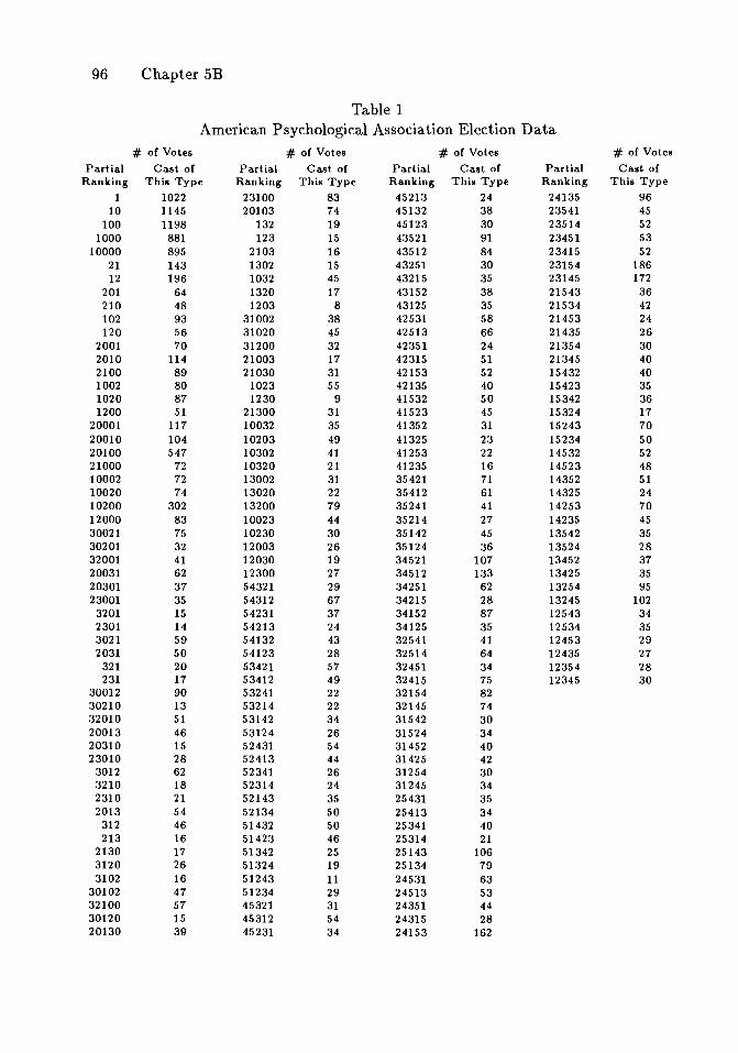
96 Chapter 5B
Table 1American Psychological Association Election Data
# of Votes # of Votes # of Votes # of Votes
Partial Cast of Partial Cast of Partial Cast of Partial Cast ofRanking This Type Ranking This Type Ranking This Type Ranking This Type
1 1022 23100 83 45213 24 24135 9610 1145 20103 74 45132 38 23541 45
100 1198 132 19 45123 30 23514 521000 881 123 15 43521 91 23451 53
10000 895 2103 16 43512 84 23415 5221 143 1302 15 43251 30 23154 18612 196 1032 45 43215 35 23145 172
201 64 1320 17 43152 38 21543 36210 48 1203 8 43125 35 21534 42102 93 31002 38 42531 58 21453 24120 56 31020 45 42513 66 21435 26
2001 70 31200 32 42351 24 21354 302010 114 21003 17 42315 51 21345 402100 89 21030 31 42153 52 15432 401002 80 1023 55 42135 40 15423 351020 87 1230 9 41532 50 15342 361200 51 21300 31 41523 45 15324 17
20001 117 10032 35 41352 31 15243 7020010 104 10203 49 41325 23 15234 5020100 547 10302 41 41253 22 14532 5221000 72 10320 21 41235 16 14523 4810002 72 13002 31 35421 71 14352 5110020 74 13020 22 35412 61 14325 2410200 302 13200 79 35241 41 14253 7012000 83 10023 44 35214 27 14235 4530021 75 10230 30 35142 45 13542 3530201 32 12003 26 35124 36 13524 2832001 41 12030 19 34521 107 13452 3720031 62 12300 27 34512 133 13425 3520301 37 54321 29 34251 62 13254 9523001 35 54312 67 34215 28 13245 102
3201 15 54231 37 34152 87 12543 342301 14 54213 24 34125 35 12534 353021 59 54132 43 32541 41 12453 292031 50 54123 28 32514 64 12435 27
321 20 53421 57 32451 34 12354 28231 17 53412 49 32415 75 12345 30
30012 90 53241 22 32154 8230210 13 53214 22 32145 7432010 51 53142 34 31542 3020013 46 53124 26 31524 3420310 15 52431 54 31452 4023010 28 52413 44 31425 42
3012 62 52341 26 31254 303210 18 52314 24 31245 342310 21 52143 35 25431 352013 54 52134 50 25413 34
312 46 51432 50 25341 40213 16 51423 46 25314 21
2130 17 51342 25 25143 1063120 26 51324 19 25134 793102 16 51243 11 24531 63
30102 47 51234 29 24513 5332100 57 45321 31 24351 4430120 15 45312 54 24315 2820130 39 45231 34 24153 162
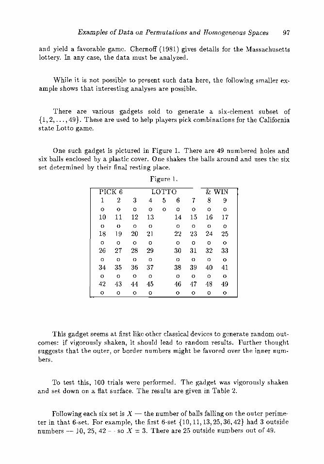
Examples of Data on Permutations and Homogeneous Spaces 97
and yield a favorable game. Chernoff (1981) gives details for the Massachusettslottery. In any case, the data must be analyzed.
While it is not possible to present such data here, the following smaller example shows that interesting analyses are possible.
There are various gadgets sold to generate a six-element subset of{I, 2, ... , 49}. These are used to help players pick combinations for the Californiastate Lotto game.
One such gadget is pictured in Figure 1. There are 49 numbered holes andsix balls enclosed by a plastic cover. One shakes the balls around and uses the sixset determined by their final resting place.
Figure 1.
PICK 6 LOTTO & WIN1 2 3 4 5 6 7 8 90 0 0 0 0 0 0 0 0
10 11 12 13 14 15 16 170 0 0 0 0 0 0 0
18 19 20 21 22 23 24 250 0 0 0 0 0 0 0
26 27 28 29 30 31 32 330 0 0 0 0 0 0 0
34 35 36 37 38 39 40 410 0 0 0 0 0 0 0
42 43 44 45 46 47 48 490 0 0 0 0 0 0 0
This gadget seems at first like other classical devices to generate random outcomes: if vigorously shaken, it should lead to random results. Further thoughtsuggests that the outer, or border numbers might be favored over the inner numbers.
To test this, 100 trials were performed. The gadget was vigorously shakenand set down on a flat surface. The results are given in Table 2.
Following each six set is X - the number of balls falling on the outer perimeter in that 6-set. For example, the first 6-set {ID, 11, 13,25,36, 42} had 3 outsidenumbers - 10, 25, 42 - so X = 3. There are 25 outside numbers out of 49.
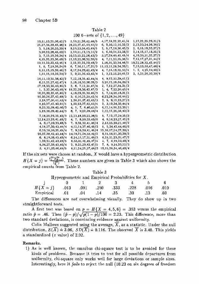
1,17,22,25,29,31/32,13,23,24,26,30/22, 6,15,18,32,37/32,14,15,17,18,35/34,10,20,31,32,37/27,13,17,27,31,44/2
19,22,28,32,42,44/27,13,19,33,47,48/41, 2, 4,15,19,40/32, 5,25,26,30,39/4
6.010.03
98 Chapter 5B
Table 2100 6-sets of {I, 2, ... , 49}
10,11,13,25,36,42/3 5,10,21,26,42,46/5 4,17,18,22,32,41/425,27,34,39,45,46/4 16,23,37,41,43,45/3 6, 9,10,12,16,32/3
3, 5,18,20,33,39/4 8,10,13,34,43,49/5 2, 5,17,19,36,40/33,10,23,26,45,49/5 2,10,11,12,13,15/2 2, 6,10,25,33,38/53, 7,15,19,26,34/4 10,13,15,22,26,43/3 3,17,29,40,41,45/44,15,32,33,36,49/3 15,19,22,30,32,39/0 4, 7,11,23,35,36/2
10,11,23,33,43,46/4 2,15,22,25,29,48/3 1,18,31,33,34,46/51, 6, 7,18,26,34/6 6, 7,10,11,17,31/3 11,13,15,28,34,39/16,11,15,19,26,46/3 6,17,24,29,42,43/4 4, 7,15,18,31,33/41,11,15,18,26,29/3 2, 9,21,36,43,45/4 1, 3,12,15,20,41/3
10,11,19,31,36,42/2 7,12,18,35,42,44/4 4, 9,12,22,39,41/36,15,25,27,42,47/4 5,16,18,33,36,39/3 3,10,12,28,34,39/3
17,18,33,36,43,46/5 2,6, 7,11,31,47/4 2, 7,12,27,34,35/31, 2,32,36,43,48/4 18,22,28,36,42,47/3 1, 4, 7,12,20,43/4
16,20,30,35,45,46/2 4,18,29,35,39,46/3 5, 7,14,16,18,31/316,20,26,37,42,49/3 3, 6,16,25,29,42/4 6,23,28,34,36,40/2
3,18,27,30,42,43/4 1,28,31,37,42,43/3 2, 5, 9,15,23,27/39,10,27,42,43,45/5 1,18,23,27,42,43/4 2, 3,19,34,39,44/46,23,32,39,42,46/3 4, 5, 7, 8,40,42/5 6,12,14,16,23,39/15,19,36,39,42,44/3 6, 7, 9,12,39,49/4 2,12,15,26,38,43/3
7,18,20,29,35,43/3 12,13,18,19,22,36/1 5, 7,12,17,29,35/312,14,23,29,41,48/2 4, 7, 8,10,33,49/6 4, 9,16,23,27,42/3
4, 6,17,20,33,48/5 7, 9,31,32,41,46/4 2,13,15,20,21,48/24,18,27,30,43,49/4 9,12,14,37,46,48/3 1, 5,34,42,44,46/66,10,18,30,35,45/4 7, 9,16,29,41,46/4 15,16,17,24,27,30/1
26,27,38,42,43,44/4 14,19,21,28,33,42/2 8,15,18,21,30,39/26, 8,19,38,43,49/4 6,14,15,17,31,49/3 6,15,21,23,32,47/21,20,25,42,43,49/5 8,33,35,41,45,47/5 5, 7, 8,19,23,49/44,34,27,39,43,46/4 2, 8,25,29,42,47/5 7, 8, 9,14,20,22/33, 4,11,33,46,49/5 8,11,24,25,37,48/3 10,15,29,34,46,49/4
If the six sets were chosen at random, X would have a hypergeometric distribution
H {X = j} = Wli:~i). These numbers are given in Table 3 which also shows the
empirical counts from Table 2.Table 3
Hypergeometric and Empirical Probabilities for X.j 0 1 2 3 4 5
H {X = j} .013 .091 .250 .333 .228 .016Empirical .01 .04 .14 .35 .30 .13
The differences are not overwhelming visually. They do show up in twostraightforward tests.
A first test was based on p = H X = 4, 5, 6} = .353 versus the empiricalratio p = .46. Then (p - p)/ p(l - p)/100 = 2.23. This difference, more thantwo standard deviations, is convincing evidence against uniformity.
Colin Mallows suggested using the average, X, as a statistic. Under the nulldistribution, E(X) == 3.06, SD(X) == 0.116. The observed X is 3.40. This yieldsa standardized (z value) of 2.92.
Remarks.1) As is well known, the omnibus chi-square test is to be avoided for these
kinds of problems. Because it tries to test for all possible departures fromuniformity, chi-square only works well for large deviations or sample sizes.Interestingly, here it fails to reject the null (10.23 on six degrees of freedom
Examples of Data on Permutations and Homogeneous Spaces 99
with all 7 categories or 9.01 on five degrees of freedom with the first and lastcategories combined).
2) Other questions can be asked of these data. To begin with, the centralnumbers
20, 21, 22, 2328, 29, 30, 31
presumably occur less often. More generally, a test that looks at all numbers, buttakes into account the distance from the edge, could be constructed. A preliminarygraphical analysis was not instructive.
Interesting questions arise about the corners and about individual numbers.With more data, some second order questions can be entertained.
3) It seems clear that this style of randomization mechanism is badly flawed.Possible physical explanations can be entertained to explain these flaws. Theballs lose most of their energy on impact with the sides, and then "trickleback" to the edge. A slight tilt draws the balls toward an edge.
4) One practical application of this kind of testing problem comes in the actuallottery. A quick test to detect marked departures is needed for a pre-gamescreening (someone might have switched for loaded balls during the night).
Example 3. Q sort data. The General Social Survey lists thirteen qualities a childcould possess. From this list, respondents are asked to choose the most desirablequality, the two next most desirable qualities, the least desirable quality and thenext two least desirable qualities. In an obvious way, this is data on SI3/SI XS2 X S7 X S2 X SI. More generally, if A is a partition of n, so A = (AI, ... , Am)with Al + ... + Am = n, one can consider data of the form: choose the first Alobjects (but do not order between), choose the next A2 objects, etc., finishingwith Am objects ranked last. Such a scheme is called Q sort data in psychologyexperiments. It is not unusual to ask for a list of 100 items to be ranked for itsdegree of concordance or similarity with a fixed object. For example, the objectmight be a person (spouse, national leader) and the items might be descriptivelevels of aggression. Suppose 9 categories of similarity are used, ranging from 1 "most uncharacteristic," through 5 "neither characteristic nor uncharacteristic,"up to 9 - "most characteristic." To aid in different rates, a forced distribution isoften imposed. For n = 100, the numbers permitted in each category are oftenchosen from binomial considerations as 5, 8, 12, 16, 18, 16, 12, 8, 5. A novelapplication and references to the older literature may be found in L. E. Moses etal (1967). For more recent discussion see Heavlin (1980).
Example 4. Other actions of Sn' The symmetric group acts on many othercombinatorial objects, such as the set of partitions or labelled binary trees. Itfollows that there is a wide variety of objects to which the analysis of this andsucceeding chapters may be applied.
c. THE d-SPHERE Sd.
Sometimes data are collected on the circle - which way do birds leave theirnests. Data are also collected on the sphere - for example, in investigating the
100 Chapter 5C
theory of continental drift, geologists looked at magnetization direction of rocksamples on two "sides" of a purported boundary. Roughly, small pieces of certainkinds of rocks have a given magnetic orientation giving points on the sphere in 1R3 •
This leads to two-sample and other data analytic problems. Such considerationsled Fisher (1953) to invent his famous family of distributions on the sphere.
Here is an example of data on higher dimensional spheres: consider testingwhether measurement errors are normal. Samples of size p are available from avariety of different sources. Say sample i is normal with parameters j.li, a}:
(X11, ... ,X1p) LLd. n(Jll,ai)
(X21 , . · ., X 2p) LLd. n(j.l2' a~)
(Xn1, ... ,Xnp) LLd. n(j.lp,a;).
Think of p small (say 10) and n large (say 50). All samples are assumed independent. Let Xi and Si be the ith sample mean and standard deviation.
The spherical symmetry of the normal distribution implies that Yi are randomlydistributed over a p - 2 dimensional sphere. Standard tests for uniformity thusprovide tests for normality.
The group of n X n orthogonal matrices O(n) acts transitively on the n sphere.The subgroup fixing a point (say the north pole (1,0,...,0)) is clearly O(n - 1).Thus the sphere can be thought of as O(n )/O(n-1) and the rich tools of harmonicanalysis become available.
Further introductory discussion is in Chapter 9B. Mardia (1972) and Watson(1983) give motivated, extensive treatments of data on the sphere.
D. OTHER GROUPS.
Many other groups occur. For example binary test results (e.g. right/wrongon the ith question 1::; i::; k) lead to data on Z~. Here, for x E Z~, f(x) is thenumber of people answering with pattern x. In panel studies a subject is followedover time. For example, 5,000 people may be followed for a year, each month aone or zero is recorded as the person is employed or not. This leads to data onZ122 •
There is a curious data set for Z365 X Z365 connected to the birthday-deathdayquestion. Some researchers claim famous people tend to die close to the date oftheir birth. See Diaconis (1985) for a review of this literature.
Data on yet other groups arises in testing Monte Carlo algorithms for generating from the uniform distribution. Such group valued random variables areuseful in doing integrals over groups. Testing a generator leads to a sample on thegroup in question. I have looked at data for the orthogonal and unitary groupsin this regard.
It seems inevitable that data on other groups and homogeneous spaces willarise naturally in applications. One final example: with many scatterplots, one
Examples of Data on Permutations and Homogeneous Spaces 101
has many covariance matrices. The set of positive definite 2 X 2 matrices isusefully represented as GL2/0 2 • Several other examples are given in the followingchapters.
E. STATISTICS ON GROUPS.
The examples described above suggest a wealth of statistical problems. Inclassical language, there is
• Testing for uniformity (is the sample really random?)• Two sample tests (is there a difference between men and women's rankings?)• Assessing association (is husband's ranking close to wife's?)• Model building (can this huge list of data be summarized by a few parameters?)• Model testing
More inclusively, there is the general problem of data analysis: how to make senseof this type of data; how to discover structure and find patterns.
The next four chapters offer three different approaches to these problems.Chapter 6 develops measures of distance on groups and homogeneous spaces.These are used to carry all sorts of familiar procedures into group valued examples.
Chapter 8 develops an analog of the spectral analysis of time series for groupvalued data. This is explored in the examples of partially ranked data. These examples make full use of the representation theory of the symmetric group. Chapter7 is devoted to a self-contained development of this theory.
Chapter 9 uses representation theory to develop a natural family of models.In familiar cases, these reduce to models introduced by applied workers. Thetheory shows how to go further, and gives a unified development for all groups atonce.
Of course, there is no substitute for trying things out in real examples, wherespecial knowledge and insight can be brought to bear. There has not been muchBayesian work on these problems that I know of. The problems of developingnatural prior distributions with respect to invariance seem fascinating. Consonniand Dawid (1985) or Fligner and Verducci (1988) offer steps in this direction.

Chapter 6. Metrics on Groups, and Their Statistical Uses
In working with data, it is often useful to have a convenient notion of distance. Statisticians have used a number of different measures of closeness forpermutations. This chapter begins by analyzing some applications. Then a hostof natural metrics (and basic properties) is provided. Next, some abstract principles for constructing metrics on any group are shown to yield the known examples.Finally, the ideas are carried from groups to homogeneous spaces.
A. ApPLICATIONS OF METRICS.
Example 1. Association. Let p be any metric on the permutations in Bn . Thus,p(1r , 1r) = 0, p(1r, u) = p(u, 1r) and p(1r, 'fJ) ::; p(1r, u) + p(u, 'fJ). Many possiblemetrics will be described in Section B. To fix ideas, one might think of p asSpearman's footrule: p(1r,u) = 2: i 11r(i) - u(i)l. One frequent use is calculationof a measure of nonparametric association between two permutations. A standardreference is the book by Kendall (1970).
As an example, consider the draft lottery example in Figure 2 of Chapter 5.The data consists of 12 pairs of numbers, (i, Yi), and Yi being the rank of theaverage lottery number in month i. It is hard to get the value of Yi out of thefigure, but easy to get the rank of Yi (i.e., biggest, next biggest, etc.). I get
1r Month I J F M A M J J A SON Du Rank Yi 5 4 1 3 2 6 8 9 10 7 11 12
The two rows can be thought of as two permutations in 812 . Are they closetogether? Taking p as the footrule, p(1r, u) = 18. Is this small? The largest valuep can take is 72. This doesn't help much. One idea is to ask how large p(1r, u)would be if u were chosen at random, uniformly. Diaconis and Graham showedthe following result (proved in Section B below).
Theorem 1. Let p(1r, u) = 2: 11r (i) - u( i) I. If u is chosen uniformly in 8n then
1AV(p) = 3"(n2
- 1)
1Var(p) = -(n + 1)(2n2 + 7)
45
{ p-AV } 1 jt 2/2P ~ t = -- e-x dx +0(1).
BD v'2i -00
In the example, AV ~ 47.7, BD ~ 9.23. The value 18 is more than 3 standard
102
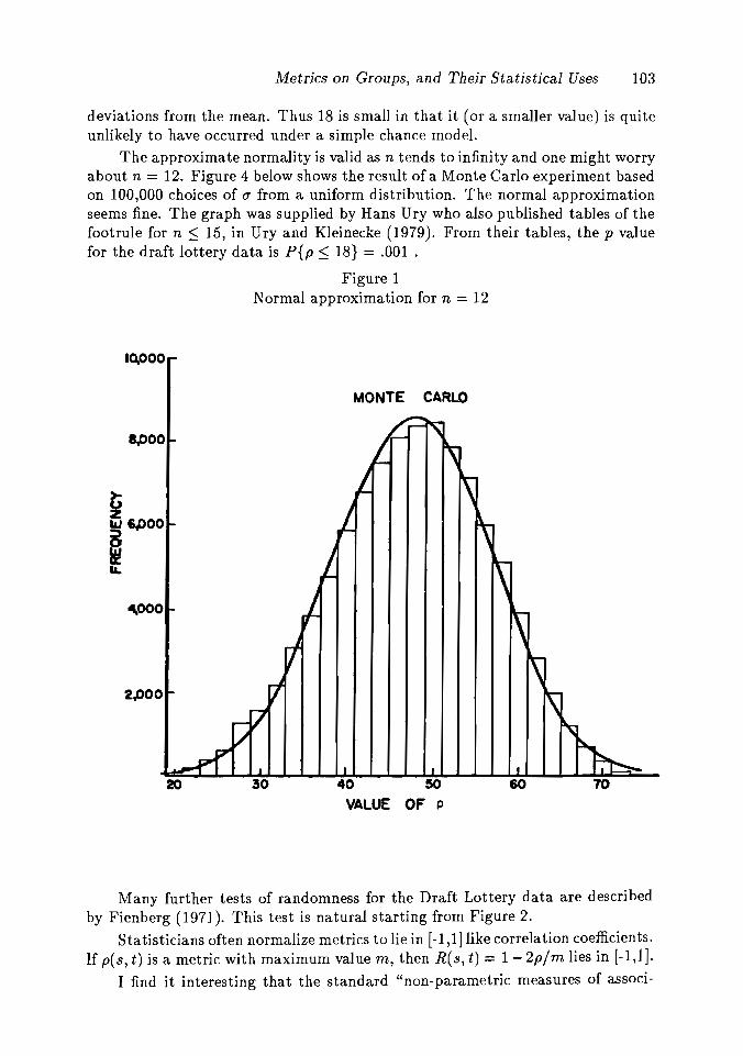
Metrics on Groups, and Their Statistical Uses 103
deviations from the mean. Thus 18 is small in that it (or a smaller value) is quiteunlikely to have occurred under a simple chance model.
The approximate normality is valid as n tends to infinity and one might worryabout n = 12. Figure 4 below shows the result of a Monte Carlo experiment basedon 100,000 choices of eT from a uniform distribution. The normal approximationseems fine. The graph was supplied by Hans Dry who also published tables of thefootrule for n ~ 15, in Dry and Kleinecke (1979). From their tables, the p valuefor the draft lottery data is P{p ~ 18} = .001 ·
Figure 1Normal approximation for n = 12
'0.000
MONTE CARLO
epoo
4.000
2.000
20 30 40 50
VALUE OF p
60 70
Many further tests of randomness for the Draft Lottery data are describedby Fienberg (1971). This test is natural starting from Figure 2.
Statisticians often normalize metrics to lie in [-1,1] like correlation coefficients.If pes, t) is a metric with maximum value m, then R(s, t) = 1- 2pjm lies in [-1,1].
I find it interesting that the standard "non-parametric measures of associ-
104 Chapter 6A
ation" arise from metrics. I've never been able to get much mileage out of thetriangle inequality, which translates to
R(s, u) ~ R(s, t) + R(t, u) - 1.
Example 2. Scaling A second use of metrics for permutation data adapts suchdata for a run through a standard multidimensional scaling or clustering program.Multidimensional scaling takes points in any metric space and finds points in theplane such that the distances between the points in the plane are close to thedistances between the points in the metric space. Imagine a collection of severalhundred rankings of 10 items. It can be hard to get a preliminary "feel" forsuch data. Scaling finds representative points or sometimes "nonlinear mapping"which can be visualized. Obviously, a metric is necessary, since the input toa multidimensional scaling program is the set of distances between the originalpoints. A nice discussion of scaling is in Chapter 14 of Mardia, Kent, and Bibby(1978). Critchlow (1985, pg. 116-121) gives an example with permutation data.Cohen and Mallows (1980) use the biplot in a similar way. See Figure 2 below.
Example 3. Mallows' model. A third use of metrics is as a means of modelbuilding. Following Mallows (1957), let's use a metric to put a probability measureon Sn. This measure will have a location parameter?ro E Sn and a scale parameterA E R+. Set
P(7r) = ce-,\p(1l",1l"o); c-1 = Le-'\P(1l",1l"o).
1r
The largest probability is assigned to ?ro and probability decreases geometricallyas the distance from ?ro. Increasing A makes the distribution more and morepeaked about ?ro. Of course, A == 0 gives the uniform distribution.
A nice application of this approach to analyzing agreement between severaljudges in a contest is in Feigin and Cohen (1978). Critchlow (1985) gives otherexamples where Mallows' model provides a good fit to ranking data.
Mallows' original derivation of this model is less ad hoc. He considers generating a ranking of n items by making paired comparisons. Suppose 1ro is thetrue ranking, but a subject errs in comparing i and j with probability p. Mallows shows that conditional on the comparisons yielding a ranking, the ranking isdistributed as above, with p given by Kendall's measure of association T and A afunction of p. This is discussed in Section B below. Fligner and Verducci (1986,1988b) develop and extend this justification for Mallows model.
Example 4. Two-sample problems. Here is a fourth use of metrics: as a meansof looking at 2 sample problems. In such problems we consider two sets of permutations 1r}, ••• , 1rnand O'}, ••• , O'm and ask about their similarities and differences.One classical question: "Can these two sets be regarded as samples from a singlepopulation of permutations?". If the 1r'S and O"s were permutations of a smallnumber of items and n and m were large, there would be no problem. The question could be treated by well-known techniques for the multinomial distribution.Consider though, the problem of distinguishing between the distribution of riffleshuffles generated by Reeds and Diaconis in Chapter 5. Here n == 100, m == 103
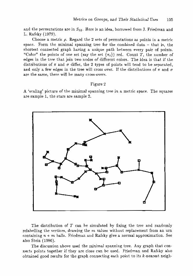
Metrics on Groups, and Their Statistical Uses 105
and the permutations are in SS2. Here is an idea, borrowed from J. Friedman andL. Rafsky (1979).
Choose a metric p. Regard the 2 sets of permutations as points in a metricspace. Form the minimal spanning tree for the combined data - that is, theshortest connected graph having a unique path between every pair of points."Color" the points of one set (say the set {1ri}) red. Count T, the number ofedges in the tree that join two nodes of different colors. The idea is that if thedistributions of 1r and (J' differ, the 2 types of points will tend to be separated,and only a few edges in the tree will cross over. If the distributions of 1r and (J'
are the same, there will be many cross-overs.
Figure 2
A 'scaling' picture of the minimal spanning tree in a metric space. The squaresare sample 1, the stars are sample 2.
The distribution of T can be simulated by fixing the tree and randomlyrelabelling the vertices, drawing the m values without replacement from an urncontaining n + m balls. Friedman and Rafsky give a normal approximation. Seealso Stein (1986).
The discussion above used the minimal spanning tree. Any graph that connects points together if they are close can be used. Friedman and Rafsky alsoobtained good results for the graph connecting each point to its k-nearest neigh-
106 Chapter 6A
bors. Critchlow (1985, Chapter 6) used the union of all minimal spanning trees for discrete metrics, the tree need not be unique.
Feigin and Alvo (1986) give another approach to assessing variability betweengroups using metrics on permutations. Fligner and Verducci (1988a) develop theseideas into a new approach for judging athletic competitions.
Example 5. Generalized association. Friedman and Rafsky (1983) have developed a method of testing association for data of the form (Xl, YI), (X2, Y2), · · · ,(x n , Yn). Here x takes values in a metric space X, and Y takes values in a metricspace Y. In an epidemiology application it might be that Xi are times of occurrence, and Yi are spatial locations of cases of a rare disease. One suspects troubleif points that are close in time are close in space.
In a more mundane setting, X and Y may both be symmetric groups, thedata representing rankings of items on two occasions.
To test "association" they suggest forming a nearest neighbor graph for theXi, and a separate nearest neighbor graph for the Yi. These graphs might bothbe minimal spanning trees. This gives two graphs on the vertex set 1, 2, ... , n.Now take T to be the number of edges that occur in both graphs. T is large ifpoints close in X are close in Y.
One can get a null hypothesis distribution for T by comparing it with repeated values from the samples (XI,Y1r(I»), ... ,(xn'Y1r(n») where 1r is a randompermutation. After all, if Xi and Yi have no connection, the value of T should beabout the same as for (Xi, Y1r(i»). Friedman and Rafsky give a normal approximation for this statistic. See also Stein (1986).
One final idea: this test of association includes the 2 sample test describedin Example 4! To see this, consider the m + n values as points in a space Y, andlet Xi be one or zero as Yi is from the first or second sample. Use the discretemetric on X. The association statistic Ta counts the number of edges that appearin both graphs. This is the number of edges in the graph in Y space that have thesame colored edges in the two sample setting. Thus T == n + m-I - Ta, so thetwo tests are equivalent; distributions are judged different if there is associationwith sample labels.
Jupp and Spurr (1985) give a different approach to testing for independenceon groups using metrics.
Example 6. Goodness of fit tests. Given a model for data in a metric space X,one can carry out standard chi-squared goodness of fit tests by splitting X intopieces based on a metric and comparing observed and expected.
Example 7. Robust regression. Here is an approach to non-linear regressionusing a metric on Sn. Consider a family of real valued functions from a space X;
f(x,O): X ~ R, 0 E 0
e.g., f(x) = a+bx, or f(x) = a+b cos (cx+d). Suppose we observe (YI,XI), ... ,(Yn, x n) and desire a value of () such that Yi is close to f(Xi, fJ). The classicalapproach to this is to fit by least squares: find a value of fJ minimizing E(Yi -
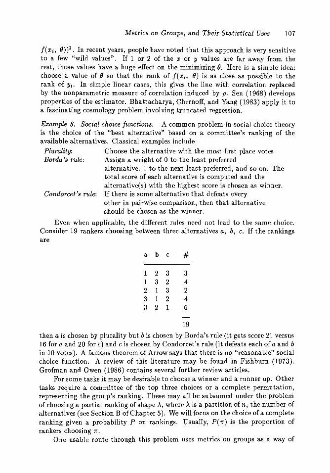
Metrics on Groups, and Their Statistical Uses 107
f(Xi, 8))2. In recent years, people have noted that this approach is very sensitiveto a few "wild values". If 1 or 2 of the x or y values are far away from therest, those values have a huge effect on the minimizing B. Here is a simple idea:choose a value of fJ so that the rank of f( xi, fJ) is as close as possible to therank of Yi. In simple linear cases, this gives the line with correlation replacedby the nonparametric measure of correlation induced by p. Sen (1968) developsproperties of the estimator. Bhattacharya, Chernoff, and Yang (1983) apply it toa fascinating cosmology problem involving truncated regression.
Example 8. Social choice functions. A common problem in social choice theoryis the choice of the "best alternative" based on a committee's ranking of theavailable alternatives. Classical examples include
Plurality: Choose the alternative with the most first place votesBorda's rule: Assign a weight of 0 to the least preferred
alternative. 1 to the next least preferred, and so on. Thetotal score of each alternative is computed and thealternative(s) with the highest score is chosen as winner.
Condorcet's rule: If there is some alternative that defeats everyother in pairwise comparison, then that alternativeshould be chosen as the winner.
Even when applicable, the different rules need not lead to the same choice.Consider 19 rankers choosing between three alternatives a, b, c. If the rankingsare
a b c #
1 2 3 31 3 2 42 1 3 23 1 2 43 2 1 6
19
then a is chosen by plurality but b is chosen by Borda's rule (it gets score 21 versus16 for a and 20 for c) and c is chosen by Condorcet's rule (it defeats each of a and bin 10 votes). A famous theorem of Arrow says that there is no "reasonable" socialchoice function. A review of this literature may be found in Fishburn (1973).Grofman and Owen (1986) contains several further review articles.
For some tasks it may be desirable to choose a winner and a runner up. Othertasks require a committee of the top three choices or a complete permutation,representing the group's ranking. These may all be subsumed under the problemof choosing a partial ranking of shape A, where Ais a partition of n, the number ofalternatives (see Section B of Chapter 5). We will focus on the choice ofa completeranking given a probability P on rankings. Usually, P( 7t") is the proportion ofrankers choosing 1r.
One usable route through this problem uses metrics on groups as a way of
108 Chapter 6A
defining a "mean" or "median". Let P be a probability on a finite group G. Letp be a metric on G. Define
f(s) = L P(t)p(s, t).t
The group element "7 is a p-median of P if "7 minimizes /(8). The number /("7) iscalled the p-spread of P. Substitution of p2 for p in the formula for /(s) yields ap-mean.
John Kemeny has proposed choosing a group ranking by using the metricinduced by Kendall's tau on Sn. In Young and Levenglick (1978), a list of properties of Kemeny's procedure are shown to characterize it. Here is a version oftheir result:
A preference function J.l assigns a set of permutations to each probabilityP on Sn. For example J.l(P) could be the set of p-medians of P. A preferencefunction is neutral if it transforms correctly under relabeling. In symbols, letPT] (1r) == P(1]- I 1r), then J.l is neutral if
/l( PT]) = 1]J.l( P) for all 1] and P.
A preference function is consistent if for any a in (0,1),
If PI and P2 represent the rankings of n and m judges respectively, then thepooled panel is represented by PIn/en + m) + P2m/(n + m). Consistency saysthat if PI and P2 lead to common preferences then the combined judges choosethese preferences.
Given a probability P, let n(P, ij) be the difference between the probabilitiesof all1r preferring i to j and all1r preferring j to i. Condorcet's proposal was thatalternative i was preferred if n(P, ij) > 0 for all j "# i (thus i would beat any j ina pairwise popularity contest).
If a complete ranking is desired, a natural extension of Condorcet's idea isthis: if i beats j in a pairwise popularity contest, then i should be ranked above jin any consensus ranking. Formally, it suffices to deal only with adjacent rankings.A preference function J.l is called Condorcet if n(P, ij > 0) (for fixed i and j) impliesno 1r with 1r(i) == 1r(j) +1 is in J.l( P). (For this, the condition becomes n(P, ij) == 0implies 1r- I (k) == i,1r- I (k + 1) == j€J.l(P) iff 1["-I(k) = j,1r-1(k + 1) == i€JL(P)).Thus, no 1r ranking j as the immediate predecessor of i is in the consensus ranking.
Young and Levenglick show that medians based on Kendall's r are neutral,consistent, and Condorcet. They further show that these three properties characterize r-medians among preference functions.
These ideas can be carried over to choosing a final ranking of shape A. Each1r E Sn can be naturally assigned to such a partial ranking. The image of P underthis map gives a probability on partial ranks and a choice of distance on partialrankings leads to a mean.
Metrics on Groups, and Their Statistical Uses 109
In Section 8.7 of Grenander (1981), a notion of a centroid set is introduced.This is very similar to a p-median, based on a distance defined using characters.
Example 9. Moments of probabilities on groups.It is not clear how the p-medians and p-spreads relate to group operations
like convolution. There is a little theory for moments of probabilities on groupsthat share, with the mean and variance, the property of being homomorphismsfrom probabilities under convolution into G (so the mean of a convolution is thesum of the means) or R+ (so the variance of a convolution is the sum of thevariances). This is elegantly surveyed in Heyer (1981).
Here is an example due to Levy (1939). Consider a random variable X takingvalues on the circle T = {zcC: Izl = 1}. Levy defined variance as
VeX) = inf f [arg(za)F Px(dz)aET iT
(where arg z is the unique cP E (-1r,1r] such that eicl> = z). Every a E T whichachieved the infimum he called a mean. He used these notions to prove thefollowing version of the Kolmogorov three series theorem: Let Xl, X 2 , ••• , be Tvalued random variables. A necessary and sufficient condition for convergence of00
L: X j a.s. isj=l
(a) EV(X j ) < 00 (b) EE(X j ) < 00
where (b) is interpreted as holding for any choice of expectations. This has beensomewhat improved by Bartfai (1966).
Note that Levy's mean is the mean of example 8, with the usual metric.
Example 10. Tests for uniformity. Let X be a homogeneous space on which Gacts transitively. We have data Xl, X2, ••• , X n and want to test if it is reasonableto suppose that these are independent and uniform.
As an example, X might equal G and the Xi might be the output of a computer routine to generate random elements of G - one wants to test such things.See Diaconis and Shahshahani (1987a) for examples.
The amount of data will play a role in choosing a test. If n is small, one canonly hope to pick up fairly strong departure from uniformity.
One simple example is the following variant of the empty cell test: Letp(x,y) be a G invariant metric. Look at m = min p(Xi,Xj), and compare withits null distribution. The null distribution can be approximated using Poissonlimit theorems for U-statistics.
To fix ideas, take X = G = zt with p(x, y) the Hamming distance - thenumber of coordinates where X and y disagree. If X and y are chosen at random,
aP{p(x, y) ~ a} = P{B(a)}, with B(a) the ball of radius a. This has L: (1) points,
j=Oa
and so P(B(a» = -:J;r L: (1)·j=O
The expected number of pairs (Xi,Xj) within distance a is thus A =(2)P(B(a)). For d large, and a chosen so that e.g. 1 ~ A ~ 10, the number
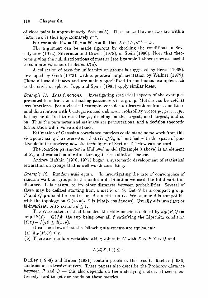
110 Chapter 6A
of close pairs is approximately Poisson(A). The chance that no two are withindistance a is thus approximately e-'\.
For example, if d == 10, n == 50, a == 0, then A == 1.2, e-'\ == .3.The argument can be made rigorous by checking the conditions in Sev
astyanov (1972), Silverman and Brown (1978), or Stein (1986). Note that theorems giving the null distributions of metrics (see Example 1 above) now are usefulto compute volumes of spheres B(a).
A collection of tests for uniformity on groups is suggested by Beran (1968),developed by Gine (1973), with a practical implementation by Wellner (1979).These all use distances and are mainly specialized to continuous examples suchas the circle or sphere. Jupp and Spurr (1985) apply similar ideas.
Example 11. Loss functions. Investigating statistical aspects of the examplespresented here leads to estimating parameters in a group. Metrics can be used asloss functions. For a classical example, consider n observations from a multinomial distribution with k categories and unknown probability vector Pt, P2, . · · ,Pk·It may be desired to rank the Pi, deciding on the largest, next largest, and soon. Thus the parameter and estimate are permutations, and a decision theoreticformulation will involve a distance.
Estimation of Gaussian covariance matrices could stand some work from thisviewpoint using the observation that GLn/On is identified with the space of positive definite matrices; now the techniques of Section D below can be used.
The location parameter in Mallows' model (Example 3 above) is an elementof Sn, and evaluation of estimators again necessitates a metric.
Andrew Rukhin (1970, 1977) began a systematic development of statisticalestimation on groups that is well worth consulting.
Example 12. Random walk again. In investigating the rate of convergence ofrandom walk on groups to the uniform distribution we used the total variationdistance. It is natural to try other distances between probabilities. Several ofthese may be defined starting from a metric on G. Let G be a compact group,P and Q probabilities on G, and d a metric on G. We assume d is compatiblewith the topology on G (so d(s, t) is jointly continuous). Usually.d is invariant orbi-invariant. Also assume d ~ 1.
The Wasserstein or dual bounded Lipschitz metric is defined by dw(P, Q) ==sup IP(f) - Q(f)l; the sup being over all f satisfying the Lipschitz conditionIf(x) - f(y)1 ~ d(x, y).
It can be shown that the following statements are equivalent:(a) dw(P,Q) ~ E.
(b) There are random variables taking values in G with X rv P, Y rv Q and
E(d(X, Y)) ~ E.
Dudley (1968) and Huber (1981) contain proofs of this result. Rachev (1986)contains an extensive survey. These papers also describe the Prohorov distancebetween P and Q - this also depends on the underlying metric. It seems extremely hard to get our hands on these metrics.
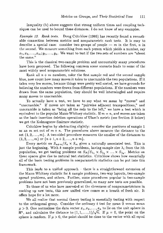
Metrics on Groups, and Their Statistical Uses 111
Inequality (b) above suggests that strong uniform times and coupling techniques can be used to bound these distances. I do not know of any examples.
Example 13. Rank tests. Doug Critchlow (1986) has recently found a remarkable connection between metrics and nonparametric rank tests. It is easy todescribe a special case: consider two groups of people - m in the first, n inthe second. We measure something from each person which yields a number, sayXl , X2, •• • , X m ; Yt, .. · , Yn' We want to. test if the two sets of numbers are "aboutthe same."
This is the classical two-sample problem and uncountably many procedureshave been proposed. The following common sense scenario leads to some of themost widely used nonparametric solutions.
Rank all n + m numbers, calor the first sample red and the second sampleblue, now count how many moves it takes to unscramble the two populations. If ittakes very few moves, because things were pretty well sorted, we have grounds forbelieving the numbers were drawn from different populations. If the numbers weredrawn from the same population, they should be well intermingled and requiremany moves to unscramble.
To actually have a test, we have to say what we mean by "moves" and"unscramble." If moves are taken as "pairwise adjacent transpositions," andunscramble is taken as "bring all the reds to the left," we have a test which isequivalent to the popular Mann-Whitney statistic. If m = n, and moves are takenas the basic insertion deletion operations of Ulam's metric (see Section B below)we get the Kolmogorov-Smirnov statistic.
Critchlow begins by abstracting slightly: consider the positions of sample 1as an m set out of m + n. The procedures above measure the distance to theset {I, 2, ... , m}. A two-sided procedure measures the smaller of the distances to{I, 2, ... , m} or {n + 1, n + 2, ... , n + m}.
Every metric on Sn+m/ Sn X Sm gives a naturally associated test. This isjust the beginning. With k sample problems, having sample size Ai from the ithpopulation, we get testing problems on S N / S Al X S)..2 X .•. X S Ak' Metrics onthese spaces give rise to natural test statistics. Critchlow shows how essentiallyall of the basic testing problems in nonparametric statistics can be put into thisframework.
This leads to a unified approach - there is a straightforward extension ofthe Mann-Whitney statistic for k sample problems, two-way layouts, two-samplespread problems, and others. Further, some procedures popular in two-sampleproblems have not been previously generalized, so many new tests are possible.
To those of us who have marveled at the cleverness of nonparametricians incooking up new tests, this new unified view comes as a breath of fresh air. Itoffers hope for a lot more.
We all realize that normal theory testing is essentially testing with respectto the orthogonal group. Consider the ordinary t test for mean °versus meanJj > O. One normalizes the data vector Xl, X2,"" X n to lie on the unit sphere inRn, and calculates the distance to (1, 1, ... , 1)/,,;n. If J-L = 0, the point on thesphere is random. If J-L > 0, the point should be close to the vector with all equal
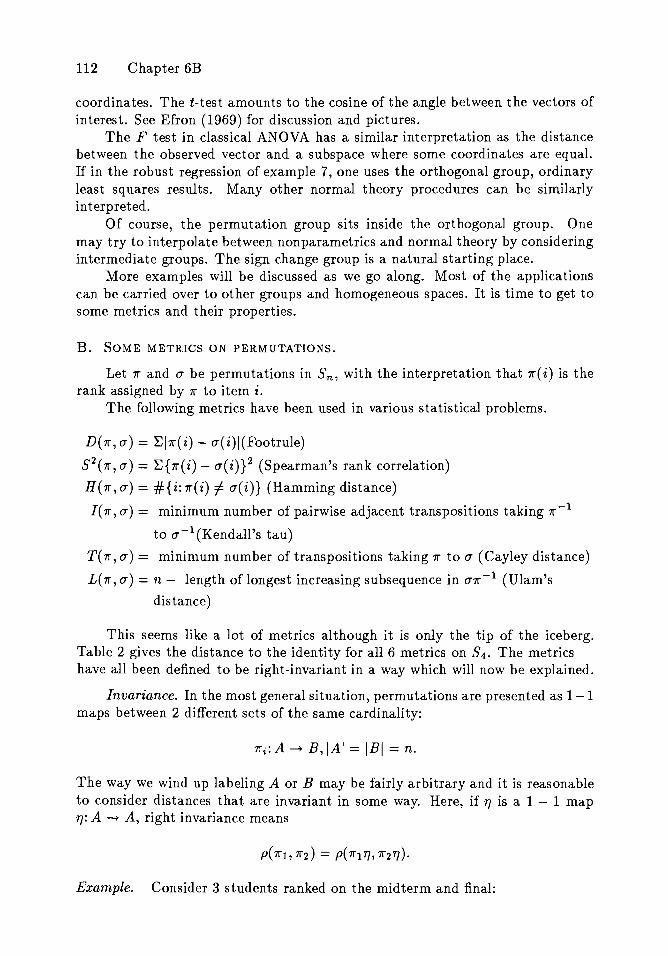
112 Chapter 6B
coordinates. The t-test amounts to the cosine of the angle between the vectors ofinterest. See Efron (1969) for discussion and pictures.
The F test in classical ANOVA has a similar interpretation as the distancebetween the observed vector and a subspace where some coordinates are equal.If in the robust regression of example 7, one uses the orthogonal group, ordinaryleast squares results. Many other normal theory procedures can be similarlyinterpreted.
Of course, the permutation group sits inside the orthogonal group. Onemay try to interpolate between nonpararnetrics and normal theory by consideringintermediate groups. The sign change group is a natural starting place.
More examples will be discussed as we go along. Most of the applicationscan be carried over to other groups and homogeneous spaces. It is time to get tosome rnetrics and their properties.
B. SOME METRICS ON PERMUTATIONS.
Let 1r and a be permutations in Sn, with the interpretation that 1r(i) is therank assigned by 1r to itern i.
The following metrics have been used in various statistical problems.
D(1r,a) = ~11r(i) - a(i)I(Footrule)
S2(1I",a) = ~{1r(i) - a(i)}2 (Spearman's rank correlation)
H(1r,a) = #{i:1r(i) =I a(i)} (Hamming distance)
1(1I",a) = minimum number of pairwise adjacent transpositions taking 1r-1
to a-I (Kendall's tau)
T(1r,a) = minimum number of transpositions taking 1r to a (Cayley distance)
L(1r,a) = n - length of longest increasing subsequence in a1r- 1 (Ulam's
distance)
This seems like a lot of metrics although it is only the tip of the iceberg.Table 2 gives the distance to the identity for all 6 metrics on S4. The metricshave all been defined to be right-invariant in a way which will now be explained.
Invariance. In the most general situation, permutations are presented as 1-1maps between 2 different sets of the same cardinality:
1ri:A ~ B,IAI = IBI = n.
The way we wind up labeling A or B may be fairly arbitrary and it is reasonableto consider distances that are invariant in some way. Here, if "I is a 1 - 1 map"I: A ~ A, right invariance means
Example. Consider 3 students ranked on the midterm and final:
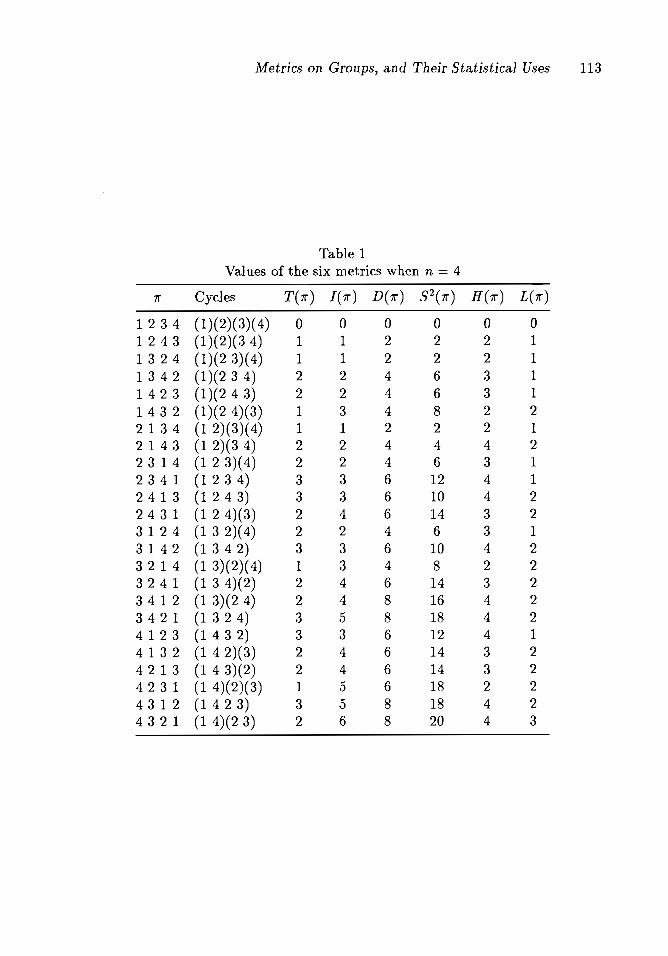
Metrics on Groups, and Their Statistical Uses 113
Table 1Values of the six metrics when n = 4
1r Cycles T(1r) I(1r) D(1r) S2(1r) H(1r) L(1r)
123 4 (1)(2)(3)(4) 0 0 0 0 0 01 243 (1)(2)(3 4) 1 1 2 2 2 11 3 2 4 (1)(2 3)(4) 1 1 2 2 2 11342 (1)(2 3 4) 2 2 4 6 3 1142 3 (1)(243) 2 2 4 6 3 1143 2 (1)(2 4)(3) 1 3 4 8 2 22 1 3 4 (1 2)(3)(4) 1 1 2 2 2 12 1 4 3 (1 2)(3 4) 2 2 4 4 4 22 3 1 4 (123)(4) 2 2 4 6 3 1234 1 (1 2 3 4) 3 3 6 12 4 1241 3 (1 2 4 3) 3 3 6 10 4 2243 1 (1 2 4)(3) 2 4 6 14 3 23 124 (132)(4) 2 2 4 6 3 13 1 4 2 (1 3 4 2) 3 3 6 10 4 2321 4 (1 3)(2)(4) 1 3 4 8 2 2324 1 (1 3 4)(2) 2 4 6 14 3 2341 2 (1 3)(2 4) 2 4 8 16 4 2342 1 (1 3 2 4) 3 5 8 18 4 24 1 2 3 (1 4 3 2) 3 3 6 12 4 14 1 3 2 (1 4 2)(3) 2 4 6 14 3 24213 (1 4 3)(2) 2 4 6 14 3 24231 (1 4)(2)(3) 1 5 6 18 2 24312 (1 4 2 3) 3 5 8 18 4 24321 (1 4)(2 3) 2 6 8 20 4 3
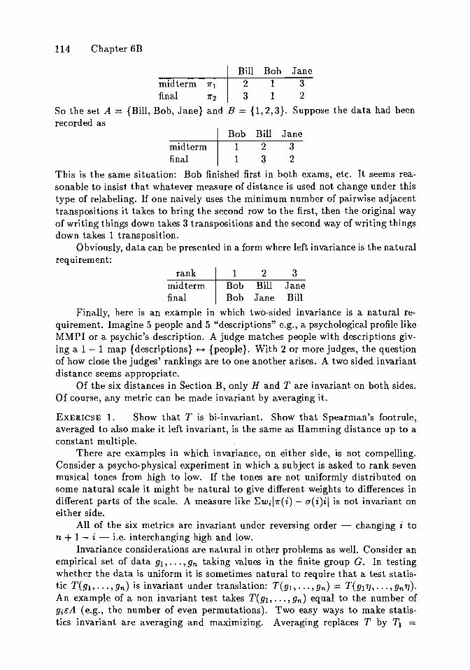
114 Chapter 6B
Bill Bob J anemidterm 7r} 2 1 3final 7r2 3 1 2
So the set A = {Bill, Bob, Jane} and B = {1,2,3}. Suppose the data had beenrecorded as
Bob Bill Janemidtermfinal
1 2 31 3 2
This is the same situation: Bob finished first in both exams, etc. It seems rea...sonable to insist that whatever measure of distance is used not change under thistype of relabeling. If one naively uses the minimum number of pairwise adjacenttranspositions it takes to bring the second row to the first, then the original wayof writing things down takes 3 transpositions and the second way of writing thingsdown takes 1 transposition.
Obviously, data can be presented in a form where left invariance is the naturalrequirement:
rank 1 2 3midterm Bob Bill Janefinal Bob Jane Bill
Finally, here is an example in which two-sided invariance is a natural requirement. Imagine 5 people and 5 "descriptions" e.g., a psychological profile likeMMPI or a psychic's description. A judge matches people with descriptions giving a 1-1 map {descriptions} ~ {people}. With 2 or more judges, the questionof how close the judges' rankings are to one another arises. A two sided invariantdistance seems appropriate.
Of the six distances in Section B, only Hand T are invariant on both sides.Of course, any metric can be made invariant by averaging it.
EXERICSE 1. Show that T is bi-invariant. Show that Spearman's footrule,averaged to also make it left invariant, is the same as Hamming distance up to aconstant multiple.
There are examples in which invariance, on either side, is not compelling.Consider a psycho-physical experiment in which a subject is asked to rank sevenmusical tones from high to low. If the tones are not uniformly distributed onsome natural scale it might be natural to give different weights to differences indifferent parts of the scale. A measure like EWil1r( i) - a( i)il is not invariant oneither side.
All of the six metrics are invariant under reversing order - changing i ton + 1 - i-Le. interchanging high and low.
Invariance considerations are natural in other problems as well. Consider anempirical set of data 91, ... , 9n taking values in the finite group G. In testingwhether the data is uniform it is sometimes natural to require that a test statistic T(91, ... ,9n) is invariant under translation: T(91,···,9n) = T(911}, ... ,9nl}).An example of a non invariant test takes T(91, ... , 9n) equal to the number of9ieA (e.g., the number of even permutations). Two easy ways to make statistics invariant are averaging and maximizing. Averaging replaces T by T1 =

Metrics on Groups, and Their Statistical Uses 115
faT~T(gl'fJ, ... ,gn'fJ). Maximizing replaces T by T2 = maxT(gl'fJ, ... ,gn'fJ).~ ~
Again, there are problems in which invariance is not compelling: In testing ashuffling mechanism for uniformity it is perfectly reasonable to pay special attention to the top and bottom cards.
We next turn to a case-by-case discussion of the six metrics and their properties.
1. Spearman's footrule D(1r,a) = ~11r(i) - a(i)l. Clearly this is a rightinvariant metric. Thus D(1r,a) = D(id,0'1r-1 ). If either 1r or (]' is uniformlychosen from Sn, the distribution of D(1r, (]') is the same as the distribution ofD(id, "I) with "I chosen uniformly in Sn. The mean of D is computed as
E{D} =~ I:D(id, IT) =~ I:t li - IT(i)1n. ~ n. ~ i=l
1 2=-en -1).3
EXERCISE 2. Prove this last assertion.A more tedious computation (see Diaconis and Graham (1977)) gives
1Var{D} = 4S(n+ 1)(2n2 + 7).
Finally, we indicate how the asymptotic normality of D can be shown (see theTheorem in example 1 of Section A for a careful statement). One approach usesHoeffding's (1951) combinatorial central limit theorem: Consider {at}, i, j =1, ... , n a sequence of arrays. Define
n
W n =L a i7l"(i)i=l
where 1r is a random permutation in Sn. Then, subject to growth conditions onafj, W n is asymptotically normal. The expression for the variance given aboveallows verification of the sufficient condition (12) in Hoeffding (1951) for the arrayaij = ti - jt, i, j = 1, ... , n. Bolthausen (1984) gives a version of the combinatoriallimit theorem with a Berry-Esseen like error bound.
Dry and Kleinecke (1979) gave tables for the foot rule when n S; 15. Theasymptotics seem quite accurate for n larger than 10. See Example 1 in SectionA above.
Diaconis and Graham (1977) give some relations between the foot rule andother measures of association that appear in the list of metrics. In particular
1+ T S; D ~ 2/.
So the more widely used metric I underlying I{endall's tau is close to the footruleD in the sense I ~ D ~ 2/.
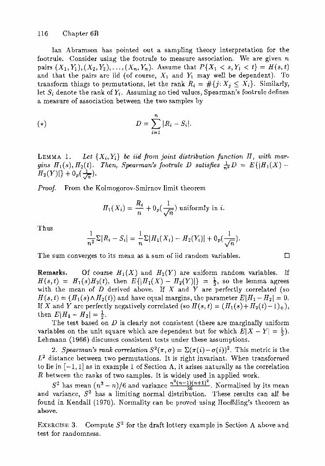
116 Chapter 6B
Ian Abramson has pointed out a sampling theory interpretation for thefootrule. Consider using the foot rule to measure association. We are given n
pairs (Xl, YI ), (X2 , 12), ... , (Xn , Yn ). Assume that P{XI < s, YI < t} = H(s, t)and that the pairs are iid (of course, Xl and Yi may well be dependent). Totransform things to permutations, let the rank Ri == #{j: X j ~ Xi}. Similarly,let Si denote the rank of Yi. Assuming no tied values, Spearman's footrule definesa measure of association between the two samples by
n
D =L IRi - Sil·i=l
LEMMA 1. Let {Xi, Yi} be iid from joint distribution function H, with margins HI(s), H2(t). Then, Spearman's footrule D satisfies ;2 D = E{IHI(X) -H 2(Y)I} +OpC)n)·Proof. From the Kolmogorov-Smirnov limit theorem
Thus
The sum converges to its mean as a sum of iid random variables. o
Remarks. Of course H 1 (X) and H 2 (Y) are uniform random variables. IfH(s, t) == HI (s)H2(t), then E{IHI(X) - H2(Y)I} == t, so the lemma agreeswith the mean of D derived above. If X and Y are perfectly correlated (soH( s, t) == (HI (s) /\ H2 ( t)) and have equal margins, the parameter EIH1 - H 2 1 == o.If X and Y are perfectly negatively correlated (so H(s, t) == (H1 (s)+H2(t)-1)+),then EIHI - H 2 1 = t.
The test based on D is clearly not consistent (there are marginally uniformvariables on the unit square which are dependent but for which EIX - YI = t).Lehmann (1966) discusses consistent tests under these assumptions.
2. Spearman's rank correlation S2(1r,a) = ~(1r(i)-a(i))2. This metric is theL2 distance between two permutations. It is right invariant. When transformedto lie in [-1, 1] as in example 1 of Section A, it arises naturally as the correlationR between the ranks of two samples. It is widely used in applied work.
S2 has mean (n3 - n)/6 and variance n2(n-;~n+l}2 . Normalized by its meanand variance, S2 has a limiting normal distribution. These results can all befound in Kendall (1970). Normality can be proved using Hoeffding's theorem asabove.
EXERCISE 3. Compute 8 2 for the draft lottery example in Section A above andtest for randomness.
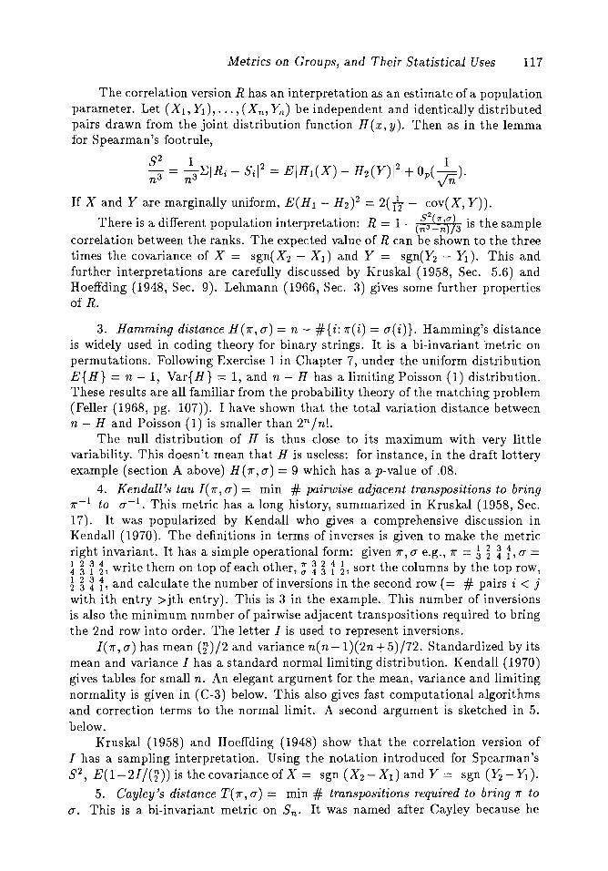
Metrics on Groups, and Their Statistical Uses 117
The correlation version R has an interpretation as .an estimate of a populationparameter. Let (Xl, Yi), ... , (Xn , Yn ) be independent and identically distributedpairs drawn from the joint distribution function H(x, y). Then as in the lemmafor Spearman's footrule,
S2 1 2 2 13 == 3L;IRi - Sil == EIHl(X) - H 2 (Y)1 + Ope c)·n n yn
If X and Y are marginally uniform, E(Hl - H 2 )2 == 2( 112 - cov(X, Y)).
There is a different population interpretation: R = 1- (~:~~)}3 is the samplecorrelation between the ranks. The expected value of R can be shown to the threetimes the covariance of X == sgn(X2 - Xl) and Y == sgn(Y2 - Yl ). This andfurther interpretations are carefully discussed by Kruskal (1958, Sec. 5.6) andHoeffding (1948, Sec. 9). Lehmann (1966, Sec. 3) gives some further propertiesof R.
3. Hamming distance H(1r,a) == n - #{i:1r(i) == a(i)}. Hamming's distanceis widely used in coding theory for binary strings. It is a bi-invariant metric 011
permutations. Following Exercise 1 in Chapter 7, under the uniform distributionE{H} == n - 1, Var{H} == 1, and n - H has a limiting Poisson (1) distribution.These results are all familiar from the probability theory of the matching problem(Feller (1968, pg. 107)). I have shown that the total variation distance betweenn - Hand Poisson (1) is smaller than 2n In!.
The null distribution of H is thus close to its maximum with very littlevariability. This doesn't mean that H is useless: for instance, in the draft lotteryexample (section A above) H(1r,a) == 9 which has a p-value of .08.
4. K endall 's tau l(1r , (J) == min # pairwise adjacent transpositions to bring1r- l to (7-1. This metric has a long history, summarized in Kruskal (1958, Sec.17). It was popularized by Kendall who gives a comprehensive discussion inKendall (1970). The definitions in terms of inverses is given to make the metricright invariant. It has a simple operational form: given 1r, a e.g., 1r == 5~ ~ t, a ==~ ~ r ~, write them on top of each other, ~ ~ ~ t ~, sort the columns by the top row,~ 5~ t, and calculate the number of inversions in the second row (== # pairs i < jwith ith entry >jth entry). This is 3 in the example. This number of inversionsis also the minimum number of pairwise adjacent transpositions required to bringthe 2nd row into order. The letter I is used to represent inversions.
l(1r, (7) has mean ('2 )/2 and variance n(n -1 )(2n + 5)/72. Standardized by itsmean and variance I has a standard normal limiting distribution. I(endall (1970)gives tables for small n. An elegant argument for the mean, variance and limitingnormality is given in (C-3) below. This also gives fast computational algorithmsand correction terms to the normal limit. A second argument is sketched in 5.below.
Kruskal (1958) and Hoeffding (1948) show that the correlation version ofI has a sampling interpretation. Using the notation introduced for Spearman'sS2, E(l- 21/(~)) is the covariance of X = sgn (X2 - Xl) and Y == sgn (Y2 - Yi).
5. Cayley's distance T(1r, a) = min # transpositions required to bring 1r toa. This is a bi-invariant metric on Sn. It was named after Cayley because he

118 Chapter 6B
discovered the simple relationship
T(1r, 0-) == n - # cycles in (1ro--l).
This is easy to prove. By invariance, take (J' == id. If 1r is a k cycle, it takes k - 1moves to sort, and disjoint cycles take separate sorting operations.
For the distribution theory, under the null hypothesis the mean is asymptotically n -log n, the variance is asymptotically log n, and T normed by its meanand standard deviation has a limiting standard normal distribution.
These results have an easy derivation. Without loss, take 0- == id. Sort 1r bytransposing pairs, first switching 1 to place 1, then 2 to place 2, etc. The chancethat 1 is already at 1 is 11n. Whether or not 1 is switched, after it is in place 1the relative order of 2, ... , n is uniform. The chance that 2 does not need to beswitched is 1/(n - 1), and so on. Thus T has the same distribution as
with XIs independent having P{Xi == 1} == 1- l/i == 1- P{Xi == O}. From here,
1 1 1 1 1 1E(T) == n - (1 + - +... + -), Var(T) == 1 + - +... + - - (1 + 22 +... + 2).
2 n 2 n n
The central limit theorem for sums of independent variables gives the limitingnormality. This proof appears in Feller (1968, pg. 257). Section C-3 below givesan algebraic connection.
The same argument works to give the distribution of the number of inversionsfor Kendall's tau. There the sum is Yl +...+Yn , with Yi uniform on 0, 1, ... , i-I.
EXERCISE 4. Compute Cayley's distance for the Draft Lottery example A-I andshow it doesn't reject the null hypothesis.
6. Ulam's distance L(1r, 0-) == n- length of longest increasing subsequence in(J'1r-
l. If (J' == § ~ r ~ ~ ~ ~ ~ ~, the longest increasing subsequence is of length 6
(e.g., 0-(3) < 0-( 4) < 0-(5) < 0-(7) < 0-(8) < 0-(9)). This natural metric is definedto be right invariant. To motivate it, consider n books on a shelf in order 0-. Wewant to sort the books by deletion-insertion-operations - taking a book out andinserting it in another place. Thus 3 moves are required to sort (J' above.
LEMMA 2. The smallest number of moves to sort 1r is n- length of longestincreasing subsequence in 1r.
Proof. If 1r( il) < 11"( i2) < ... < 11"(ik) is a longest increasing subsequence, thenclearly inserting and deleting other letters doesn't change the ordering of thissubsequence. It follows that n - k moves suffice. Since each move can increasethe longest increasing subsequence by at most 1, n - k moves are required. 0
This metric is used by biologists and computer scientists. See I(nuth (1978,5.1.4). Gordon (1983) has suggested it for statistical tasks. If n is large, it is
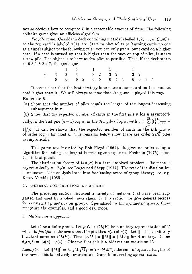
Metrics on Groups, and Their Statistical Uses 119
13 26 547
13 2654
13 26 5
36
6
not so obvious how to compute L in a reasonable amount of time. The followingsolitaire game gives an efficient algorithm.
Floyd's game. Consider a deck containing n cards labelled 1,2, ... , n. Shuffle,so the top card is labeled 1r(1), etc. Start to play solitaire (turning cards up oneat a time) subject to the following rule: you can only put a lower card on a highercard. If a card is turned up that is higher than the ones on top of piles, it startsa new pile. The object is to have as few piles as possible. Thus, if the deck startsas 6 3 1 5 2 4 7, the game goes
1 13 3665
It seems clear that the best strategy is to place a lower card on the smallestcard higher than it. We will always assume that the game is played this way.
EXERCISE 5.(a) Show that the number of piles equals the length of the longest increasing
subsequence in 1r.(b) Show that the expected number of cards in the first pile is log n asymptoti-
00 .
cally, in the 2nd pile (e - 1) log n, in the 3rd pile clog n, with c = L: [(;J) j~l -j=l
1]/j!. It can be shown that the expected number of cards in the kth pile isof order log n for fixed k. The remarks below show there are order 2Vn pilesasymptotically.
This game was invented by Bob FIoyd (1964). It gives an order n log nalgorithm for finding the longest increasing subsequence. Fredman (1975) showsthis is best possible.
The distribution theory of L(1r,a) is a hard unsolved problem. The mean isasymptotically n - 2Vn, see Logan and Shepp (1977). The rest of the distributionis unknown. The analysis leads into fascinating areas of group theory; see, e.g.Kerov-Vershik (1985).
C. GENERAL CONSTRUCTIONS OF METRICS.
The preceding section discussed a variety of metrices that have been suggested and used by applied researchers. In this section \ve give general recipesfor constructing metrics on groups. Specialized to the symmetric group, theserecapture the examples, and a good deal more.
1. Matrix norm approach.
Let G be a finite group. Let p: G ~ GL(V) be a unitary representation of Gwhich is faithful in the sense that if s =1= t then p(s) =1= p(t). Let" " be a unitarilyinvariant norm on GL(V). Thus "AMII = IIMII = IIMAII for A unitary. Definedp(s, t) = IIp(s) - p(t)ll. Observe that this is a bi-invariant metric on G.
Example. Let IIMII2 = 'Ei,jMijMij = Tr(M M*), the sum of squared lengths ofthe rows. This is unitarily invariant and leads to interesting special cases.

120 Chapter 6C
Case 1. Take G = Sn. Take p as the n-dimensional permutation representation.Then, d~(id,1r) = Tr(I - pCrr))(I - p(7r)T) = Tr(21 - p(7r) - p(1r)T) = 2H(id,7r)where H is the Hamming metric, where on the right, dp is the dimension of p.
Case 2. For general G and p, the argument above shows that characters yieldmetrics. Thus dp(s, t) = (d p- re Xp( st- l )) t is a metric, where on the right, dp isthe dimension of p.
Case 3. Specializing the above to the usual n-dimensional representation ofthe orthogonal group, dp(s, t) = (n - Tr(st- l ))t is a metric on On. Considerthe distance to the identity d( s, id) = Jn - Tr( s). The (i,i) element of s is thecosine of the angle between sei and ei, where ei is the ith basis vector. Thusd(s, id) = {L;l- (sei,ei)}t. Since the metric is bi-invariant, it can be expressedin terms of eigenvalues e iBj : d( s, id)'= {L;(1 - cos Bj)}!.
Despite these natural properties, and its ease of computation, this is notthe "natural" metric on On. Mathematicians prefer a metric arising from theRiemannian structure on On as a Lie group. In terms of the eigenvalues thismetric is {~B]}t. See E-5 below.
Case 4. The regular representation R of G gives the discrete metric
if s i= tif s = t.
To determine the distribution of dp(id, t) requires knowing the distribution ofcharacters. That is, pick t at random on G, and treat Xp(t) as a random variable.This is a problem that is interesting on its own. It has not been well studied.
EXERCISE 6. Show that E(Xp) and E(Xp - EXp)(Xp - EXp) can be expressedas follows: Let XP = alXl +...+ahXh be a decomposition into irreducibles, withrepetitions. If Xl is the trivial representation, then E(Xp) = aI, and E(Xpx.p ) =ai + · . ·+a~. In particular, if p is real irreducible, E(Xp) = 0, Var(xp) = 1. Findthe mean and variance of d~ described 'in Case 4 above.
Remark. Exercise 6 suggests that metrics defined as (d p - re X(st- l ))! willnot be very "spread out." For real irreducible representations, d~ has mean dimp and variance one. Nonetheless, they can have interesting distributions. Forexample n - H(id,1r) has a limiting Poisson(l) distribution. Further, the firstn moments of n - H(id,1r) equal the first n moments of Poisson(l). Similarly,the first 2n + 1 moments of the trace of a random orthogonal matrix equal thefirst 2n + 1 moments of a standard normal variable. Thus, the distance definedfor the orthogonal group (Case 3 above) has an approximate standard normaldistribution. See Diaconis and Mallows (1985) for these results.
EXERCISE 7. Take G as Sn. Let p be the ('2') dimensional representation derivedby the action of 7r on the set of unordered pairs {i, j}. Show that for large n, Xp( 7r)has as limiting distribution the same distribution as X(~ -1) + Y where X and Yare independent, X is Poisson(l) and Y is Poisson(1/2).
Metrics on Groups, and Their Statistical Uses 121
EXERCISE 8. Compute distances suggested by the discussion above for G = Zn,and Z:r. What are the limiting distributions for n large?
All of the above examples used the L 2 or Frobenius norm. There are manyother unitarily invariant norms. Indeed, these have been classified by von Neumann (1937). To state his result, define a symmetric gauge function as a function</>: Rn -+ R satisfying(a) 4>(Ut, · · · , un) 2:: 0, 4> continuous.(b) 4>(Ut, · .. , un) = 0 implies Ut = ... = Un = o.(c) </>(tUt, ... , tUn) = t</>(Ut, . .. , Un), t ~ o.(d) </>(Ut +ui ,... Un + u~) ~ </>(Ut, ... , Un) + </>(ui , ... , U~).(e) </> is invariant under permuting and sign changes of coordinates.
For M E GL n , let Wt, ... , W n be the eigenvalues of M M* . Define"M 11
</>(IWtl!, ... ,lwnl!). This is a matrix norm: II cM JI = IcIlIMII,IIAl + Nil <II M II + IINII. It is unitarily invariant and IIMII = IIM*II.
Von Neumann showed that, conversely, every such norm arises in this way.Examples include
4>= (:ElwiI P);', maxlwil, or { L WitWi2' "Wij7.
il~i2... ~ij
The first of these, for p = 2, becomes the already considered matrix norm(ErMiir2)t. The second choice becomes the maximum length of Mu subjectto uut = 1. These last two norms also satisfy IIMNII ~ IIMIIIINII. It would beinstructive to try some of these norms out on the symmetric group.
2. The fixed vector approach.
Let G be a group, (p, V) a representation. Suppose that V has an innerproduct, and p is unitary. Fix a vector v E V and define
This distance has been defined to be right invariant. It clearly satisfies the triangleinequality and symmetry. One must check that d(id, t) =I 0 unless t = id. It isnot even necessary that 1111 come from an inner product. All that is needed is thatp(s) be norm preserving for s E G.
Example. Take G = Sn, p the usual n-dimensional representation, so p(1r- t )
(Vt,V2, ••• ,Vn) = (V1r(1),V1r(2), ••• ,v1r(n»). Take v = (1,2, ... ,n)T. Then d2(1r,fJ)= ~11r(i) - 'f](i)1 2 • If the distance on Rn is chosen as the L 1 distance, Spearman'sfootrule results. These considerations emphasize that Spearman's rho and footruledepend on the choice of v. They make it easy to change v to emphasize differencesat one end of the scale. The distribution theory of these variants follows fromHoeffding's combinatorial limit theorem. The strong points of the fixed vectorapproach will become apparent when it is applied to homogeneous spaces in thenext section.
122 Chapter 6C
3. Lengths.
Let G be a finite group. Let S be a subset of G that generates G in the sensethat any element can be written as a finite product of elements in S. Assume idfj. Sand S-1 = S. Define the length of an element t as the smallest integer q ~ 0such that t = 8182 .. . 8 q with each 8i E S. Write q = R.( t). Thus id is the uniqueelement of length zero, and each element of S has length 1.
Define a metric on G by d(t, u) = f(tu- l).
LEMMA 3. The length metric d( t, u) = f( tu-1 ) is a right invariant metric. It istwo-sided invariant if tSt- l = S for every t E G.
Proof. Clearly, lengths satisfy R.( tu) ~ R.( t) +f( u), and f( t) = R.( t- l). Thus d( t, u)
is a right invariant metric. For the last claim, d(T/t,T/u) = R.('fJtu- l 'fJ-l) = f(tu- l )
because S is invariant under conjugation by "I. 0
Example. Take G = Sn. If S is chosen as the set of all transpositions one getsthe Cayley metric T. Choosing S as the set of transpositions of form (i, i + 1), 1 ~i ::s; n - 1 gives the metric form I of Kendall's tau. To get Ulam's metric L, takeSI as the set of all cycles (a,a + 1, ... ,b),1::S; a < b ~ n. Let S = SI U S1 1
.
These amount to the basic insertion deletion operations described in example 6of Section B.
Not all metrics arise this way. For instance, the Hamming distance on Sn isnot based on lengths. To see this observe that elements in S have length 1 andtwo permutations cannot disagree in only one place. The Hamming distance onZ2 is based on lengths.
There is a curious application of some fairly deep group theory to the distribution theory of length metrics. When specialized, it gives the neat representationsof Kendall's and Cayley's distances as sums of independent random variables.
Each of the classical groups (e.g. orthogonal, unitary, symplectic) has associated a finite Weyl group W. A Weyl group is a group W with a set of generators81, 82, ... ,Sn such that sr = id and for some integers nij, (8i' 8 j )nij = id, thesebeing the only relations. For example, Sn with generators (i, i + 1) is a Weylgroup; nij being 2 if the generators are disjoint and 3 otherwise. The sign changegroup (permute coordinates and change signs arbitrarily) is another familiar Weylgroup.
Modern motivation for studying these groups comes from Lie theory andcombinatorics. Bourbaki (1968) and Stanley (1980) are readable surveys.
Let (W, S) be a Weyl group. Let F(t) = ~WEwti(w) be the generating function of the lengths. A basic theorem in the subject states that there exist an mand integers ei called the exponents of W such that
m
F(t) = II(1 + t+ ... te;).
i=l
Letting t = 1, this shows IWI = II(ei + 1). Dividing both sides by IWI, we havethe following.
Metrics on Groups, and Their Statistical Uses 123
COROLLARY 1. Let (W, S) be a Weyl group with exponents ei. Then the lengthof a random w E W has the distribution of Xl + + X m , where the Xi arechosen as independent uniform variables on {O, 1,2, , ei}.
The factorization can be found as Exercise 10 of Section 4 in Bourbaki(1968) or Stanley (1980). As a convolution of symmetric unimodal distributions,P{l(w) = j} is a symmetric unimodal sequence as j varies.
As an example, on Sn with pairwise adjacent transpositions as generators,the exponents are ei = i-I for i = 1,2, ... , n, and the factorization becomes therepresentation of the number of inversions as a sum of uniforms discussed underCayley's distance in Section B above.
There is a second general theorem of the same type. Let (W, S) be a Weylgroup. Take S = {tSt- l } as a new set of generators obtained by closing up theold set under conjugation. This gives a new length function, say f( w). It is anamazing fact that the generating function of f factors as
m
L i(w) = IT(1 +ejt).w i=l
COROLLARY 2. Let (W, S) be a Weyl group with exponents ei. Then the length"lof a random w E W has the distribution ofXl +.. .+Xm where Xi are independentwith P{Xi = O} = 1/1 + ei, P{Xi = 1} = ei/ 1 + ei.
The factorization (*) was proven by Coxeter and Shephard Todd. SeeSolomon (1963) or Proposition 4.6 in Stanley (1979).
These representations make the means and variances of d( s, t) easy to compute. They also make the distribution easy to work with: sums of independentuniforms have an easy limit theory, with correction terms readily available. Further, Harding (1984)'shows how such factorizations lead to an easy algorithm forfast exact computation of distributions in small cases.
Of course, in the case of Cayley's distance or Kendall's tau, the representations are well known in statistics. In the next section we show how a similarfactorization holds for the natural extension of these metrics to homogeneousspaces.
EXERCISE 9. Consider Hamming distance on Z!f. Show its length generatingfunction factors as (1 + t)n.
An Application. Here is an application of the factorizations in Corollaries1 and 2 above. Consider Monte Carlo generation of a sample from the Mallowsmodel (example 3 of Section A) based on the metric I of Section B:
*
We begin by recalling a correspondence between permutations and sequences.Let (at, ... , an) be a sequence of integers 0 ~ ai ~ i -1. Associate a permutationby insertion; starting with n, n - 1, n - 2, ... insert n - i +1 so it has ai previously
124 Chapter 6D
inserted numbers to its left. Thus, if n = 7, the sequence (0,0,1,3,2,3,6) developsas
7 --+ 67 --+ 657 --+ 6574 ~ 65374 --+ 653274 --+ 6532741.
The final permutation has al +.. .+an inversions (here 15). This gives a 1-1 correspondence between permutations and sequences, with the sum of the sequenceequal to the number of inversions. The correspondence is equivalent to the Weylgroup factorization of Corollary 1 above.
If the initial sequence is chosen uniformly: 0:::; ai :::; i-I, then a randompermuta.tion results. If P{ai = j} = e->'i[ :~;i-=-;]' 0 :::; j :::; i - 1, the fina.lpermutation has probability * with 11""0 = id. The distribution of ai is easy togenerate by inversion (Chapter 111.2 of Devroye (1986)).
It is easy to modify things to incorporate 11""0, or to work for any other metricwith a similar factorization.
Fligner and Verducci (1986, 1988b) have pointed out that the normalizingconstant C(A) in * is known from the factorization in Corollary 1. They apply this in doing maximum likelihood estimation and as a way of extending themodels. Steele (1987) discusses some other combinatorial problems where similarfactorizations arise.
D. METRICS ON HOMOGENEOUS SPACES.
Most of the considerations of previous sections can be generalized to homogeneous spaces. Let X be a homogeneous space on which a group G operatesfrom the right, transitively. Fix fio E X, let l( = {s E G: Yos = Yo}. In thissection X will be identfied with right cosets of l( in G, X ~ {l(Xi} where id =Xo, Xl, ... , Xj E G are coset representatives for l( in G (so G = !( U!(Xl ... ul(Xj
as a disjoint union). Here G acts (from the right) on cosets by xs = (l(x)s = l(xsfor any s E G and any x = l( X EX.
We have made a slight change of notation (from left to right cosets) to agreewith the notation in Critchlow (1985). Critchlow's monograph develops a host ofmetrics for partially ranked data. He gives numerous applications, computer programs, and tables for popular cases. It is very readable and highly recommended.
There are several ways to choose a metric on X which is right-invariant inthe sense that d(x,y) = d(xs,ys), Le. d(l(x,l(y) = d(l(xs,l(ys).
a) Hausdorff metrics. Let G be a compact group, l( a closed subgroup andd a metric on G. Let X be a space on which G acts transitively with isotropysubgroup l(. Write X = G/ l( to denote the representation of X by right cosets.
A metric d* is induced on G / l( by the formula
d*(x,y) = d*(l(x,l(y) = max(a,b)
witha = max min d(s, t), b = max min d(s, t).
sE!( x t E!( y sE!( y t E!( x
The metric d* is the Hausdorff distance between the sets l(x and l(y - thesmallest amount that each must be "blown up" to include the others. It is a
Metrics on Groups, and Their Statistical Uses 125
standard way to metrize the homogeneous space X, see e.g., Dieudonne (1970,pg. 53), Nadler (1978), or Roelcke and Dierolf (1981).
EXERCISE 10.(a) Show that d* is a metric.(b) If d is right invariant then so is d*.(c) If d is left invariant, then d*(!( x, !(y) = min d( x, ky).
kE!(The definition of d* seems more theoretically than practically useful - it
seems hard to explicitly compute the minimum. However, Critchlow (1985) hasgiven reasonably elegant closed form expressions for partially ranked data and dany of the classical metrics of Section B. Some of his results will be given here.
Example 1. k sets of an n set. Let x and 11 be k element subsets of {I, 2, ... , n}.Note x and fi can be identified with points in the homogeneous space Sn/(Sk X
Sn-k), where Sk X Sn-k is the subgroup {1r E Sn:7r(i) ~ k Vi = 1, ... ,k and1["(i) > k Vi = k + 1, ... , n}. Let H be the Hamming distance on the symmetricgroup Sn. Then the induced Hausdorff metric is
H*(x, y) = 2(k - Ixn Yl).
To see this, realize x and y as ordered sets Xl < ... < Xk, YI < ... < Yk. Associate permutations x and y to x and y by choosing coset representatives. SinceH(x,y) = H(x-1,y-l), the permutations can be taken as
y = (YIY21 2
Xk x~
kk+l
Yk yikk+l
Now using part c) of the exercise above
H*(x, y) = min H(x, 'fry).'TrESIe xSn-1e
Multiplying on the left by 'fr allows us to permute the Yi with i E {I, ... , k} amongthemselves and the Yi' E {k + 1, ... , n} among themselves in the first row of y.This permits matching elements and proves the result.
The null distribution of IxnVI is the well known hypergeometric distribution.
Example 2. Rank k out of n. Here people rank order their favorite k out of n, inorder. Represent a ranking as (Xl, X2, • •• , Xk) where Xl is the item ranked first,X2 is the item ranked second, etc. Critchlow (1985, Chapter 3) shows
H*(x, y) = #{i ::; k: Xi # Yi} + (k -Ixn Vi)·
Again, this is a very reasonable distance, albeit, perhaps, a bit crude.Critchlow gives similar explicit, interpretable formulas for the induced Hausdorffdistances derived from the other classical metrics.
126 Chapter 6D
Example 3. The n-sphere. Using the distance d2( s, t) == n - Tr( st- 1
) on theorthogonal group, then choosing reflections I - 2xxt as coset representatives (forx on the unit sphere), leads to
Diaconis and Shahshahani (1983, Sec. 3) discuss the choice of coset representativesmore carefully. If x or y is chosen at random, Vfi,(d2 -1) is approximately standardnormal for large n. This last result is proved with good error bounds in Diaconisand Freedman (1987).
b) The fixed vector approach. Here is another large class of invariant metricson a homogeneous space X == G/ l(. Let (p, V) be any unitary representation ofG. Say p has a l( fixed-vector v E V if p(k)v == v for every k E l(. Usually it iseasy to find such a p and v, see the examples below. It follows from Chapter 3Fthat p has a l( fixed vector if and only if p appears in the decomposition of L(X).Define a metric on X by
Note that this is well defined (it is independent of the choice of coset representatives). Note further that this distance is right G-invariant:
dp(xs, ys) == dp(l( xs, l( ys) == IIp(s-l )[p(x-1) - p(y-1 )]vl/
== dp(x, y),
because p is unitary. This dp clearly satisfies the properties of a metric exceptperhaps for dp(x, y) == 0 implying x == y. This must be checked separately. Thefixed vector approach was suggested by Andrew Rukhin as a way to choose lossfunctions in statistical problems on groups.
Example 1. k sets of an n set. For the (k) k-element subsets of{1,2, ... ,n},choose p as the usual n-dimensional representation on Rn with the usual innerproduct. Take v == (a, ... , a, b, ... , b) with a run of k a's followed by n - k b's.Choosing coset representatives as the reverse shuffles of example 1 above yields
Cf. Example 1 of the Hausdorff approach.Again, Critchlow (1985) gives a variety of results, giving extensions of Spear
man's foot rule and rho to partially ranked data.
Example 2. The n-sphere. Take X == sn G == On, l( == On-1. Take p as theusual n-dimensional representation of On, and e1 == (10 .. .O)t as a le-fixed vector.Finally take coset representatives as I - 2vvt where v == (e1 + x)fc,c == le1 +xl,and x runs over sn. An easy computation yields d2(x, y) == /Ix _ yl/2.
Constructions a, b, make it clear that there are a wealth of tractable metrics on homogeneous spaces. Critchlow gives examples and applications carrying
Metrics on Groups, and Their Statistical Uses 127
over much of the material of Section A to partially ranked data. He has subsequently developed many further applications to standard nonparametric problemsas remarked in Example 13 of Section A.
There are a reasonable number of nice distributional problems open - thenull distribution of metrics on homogeneous spaces needs to be better developed.The following special case hints at what's lurking there.
Example. A metric on partially ranked data. Consider six flavors, a, b, c, d,e, f.Suppose two rankers rank them, choosing their two favorites, and two least favorite, not distinguishing within:
(1) a bed e f1 212 3 3
a bed e f1 1 332 2
How close are these ranks? It is natural to try the minimum number of pairwiseadjacent transpositions it takes to bring one bottom row to the other. This is 5in the example. Recall however that the labelling of the top row is arbitrary. Thetwo arrays could just as easily have been presented with first and last columnsswitched. This yields
f bed e a3 2 1 2 3 1
f bed e a2 1 3 3 2 1
These are the same rankings, but now their distance is 3.A simple way to have invariance rearranges the two rankings in order of (say)
the first, and then computes inversions. Thus (1) becomes
a c b d e f112 233
a c b d e f131 322 # inversions = 5.
If we had sorted by the 2nd ranking (1) becomes
a b e fed1 233 1 2
a b e fed1 1 2 2 3 3 # inversions = 5.
This example has n = 6, and partial rankings of shape 222. More generally,
Definition. Let A be a partition of n. Let 1r and'TJ be partial rankings of shape A.Define l( 7r , TJ) as follows: arrange the columns of 7r and 1] so that 7r is in order,beginning with Al ones, A2 twos, etc. This must be done using the minimumnumber of pairwise adjacent transpositions. Then count the minimum number ofpairwise adjacent transpositions required to bring the 2nd row of 'TJ into order.
EXERCISE 11. Show that I is a right invariant metric.One reason for working with the metric I is the following elegant closed form
expression for its null distribution. By right invariance, this only needs to be
computed for l( id, 1r) ~ l(n).
Theorem 2. Let A = {AI, A2' ... , Ar } be a partition of n. Let 7r range over then!/IIAi! partial rankings of shape A. Then
128 Chapter 6D
where ((A))! = ((A - l))((A - 2)) ... ((1)) with ((j)) == 1+ q + q2 +... + qj-1.
Remarks. Theorem 2 was proved by Netto when r == 2, and by Carlitz inthe general case. Stanley (1985, Proposition 1.3.17) presents several elementaryproofs. Stanley (1980) proves that the coefficients P{l(1r) == j} are symmetricand unimodal. The factorization and unimodality generalize to other Weyl groups.The expressions on the right side are known as q-nomial coefficients.
Fligner and Verducci (1986, 1988b) use this factorization as a base for extending and interpreting Mallows model on partially ranked data.
Note that « A) )!j A! is the generating function of the convolution of A independent uniform variables U1 + ... + U).. with Ui uniform on {O, 1,2, ... , i - 1}.This gives an easy way to compute means, variances, and asymptotic distributions where necessary. The following neat argument evolved in work with AndyGleason and Ali Rejali. For clarity, it is given for A == (k, n - k).
The null distribution can be described this way: let x be a pattern of k onesand (n - k) twos. Let l(x) be the number of inversions (e.g. 2121 has 3 inversions).For x chosen at random, the generating function of l( x) satisfies
~~ qI(x) _ «(k))(k) x - (k) ·
Rearranging, the right hand side is
gn(q)gn-l(q) gn-k+l(q)
9k(q)9k-l(q) g2(q)
with 9j(q) == t(l + q + ..'. + qi-1), the generating function of Uj - a uniform
random variable on {O, 1,2, ... j - 1}. This has mean == Ilj == j;l and variance2 _ j'2_1
(J' j - 12 ·
Cross-multiplying, the identity has the probabilistic interpretation
D1 +U2 +U3 + ... + Uk == Un + Un- 1 +... + Un-k+l,
where the D means equality in distribution. All of the uniform variables areindependent. From this we have
PROPOSITION 1.) E(l) - + - k(n-k)
a - Iln · · · + Iln-k+l - Ilk - Ilk-I· · · - J-L2 - 2
b) V (1) - 2 2 2 2 2 _ k(n+1)(n-k)ar - (J'n + · · ·+ (J'n-k+l - O'k - O'k-1 · . · - 0'2 - 12
c) As nand k tend to infinity in any way, provided n-k also tends to infinity, thedistribution of I, standardized by its mean and standard deviation, has a standardnormal limit.
Proof. The mean and variance are derived in the remarks preceding the statement. For the distribution, suppose without loss that k ~ n/2. Write the distributional identity as I + Uk == Un-k. Then standardize
{I - Ill} _(1l + {Uk~ JIk} _7h g Un-k - JIn-k0'1 O'n-k O'k O'n-k an-k
Metrics on Groups, and Their Statistical Uses 129
The right side converges to a standard normal distribution, as does {Uki,Tik}.Since this last is independent of { [:11
}, it must be that { [:11 } converges, andby Cramer's theorem, to a standard normal. 0
Remark 1. The argument above works for virtually any type of partition, inparticular 1q, (n - q)l - for rankings of q out of n.
Remark 2. The proof is similar to the standard argument for the Mann-Whitneystatistic given in I<:endall and Stuart (1967, pg. 505).
Remark 3. The generating function is a ratio of generating functions. We tookadvantage of this by cross-multiplying. That is different from having a directprobabilistic interpretation. Indeed, I do not know how to generate random partialrankings from the associated Mallows model as suggested for full rankings at theend of the last section. Fligner and Verducci (1988b, Sec. 3.2) have made someprogress here.
E. SOME PHILOSOPHY.
We have seen examples and applications of metrics. We pause for a momentto reflect on the big picture. What makes a natural metric; how can we comparemetrics? Important issues here are
1) Interpretability. Is the metric easy to think about directly, easy to explainto a non-professional? Does it measure something with real world significance suchas the actual number of steps required to sort, or the running time of an algorithm,or the cost of an error?
Along these lines, observe that Cayley's, I<:endall's tau, and Ulam's metrichave sorting interpretations. The footrule, Kendall's tau, and Spearman's rhohave a statistical interpretation as estimates of population parameters.
2) Tractability. Is the metric easy to compute? The footrule, Hamming andrho are trivial to program, Cayley and tau require a bit of thought, and Ulam'smetric can be tricky if n is large. Is the null distribution available for smallsamples? Are useful asymptotics available? Ulam's metric fares badly here - itsasymptotic distribution is unknown. Of course, null distributions can always besimulated.
3) Invariance. In the application, is right or left invariance natural andavailable?
4) Sensitivity. Does the metric effectively use its range or does it just take ona few values? Among two sided invariant metrics this is a problem. Worst is thediscrete metric (d(s, t) = 0 or 1 as s = t or not). Next is Hamming distance, whicheffectively takes on only a few values around n under the uniform distribution.Finally, Cayley's distance takes about v'log n values effectively. It should bepossible to find bi-invariant metrics that naturally take on more values. Sincevariance can be changed by multiplication by a constant, perhaps the limitingcoefficient of variation J-L/ (J' should be used to measure effective range.
5) Available theory. Has the metric been studied and used enough so that itsstrengths and pitfalls are known? Does it link into other aspects of the analysis?
130 Chaptper 6E
A nice example arises for continuous groups. Mathematicians seem to agree ona unique bi-invariant way of metrizing Lie groups such as the orthogonal group.When pushed "what makes that metric so natural?" they respond with theoremslike "there is a unique differential (smooth except at id, like Ixl) bi-invariantmetric compatible with the Riemannian structure." See Milnor (1976, Lemma7.6). Metrics can sometimes be derived from axioms (as in Example A-8).
6) The bottom line. There is a fairly harsh test: did somebody actually usethe metric in a real application? Was it used to prove a theorem? Could this havebeen done without the metric just as easily? Failing this, does the metric lead tointeresting theoretical questions or results?
A first pass through this list suggests Kendall's tau as the metric of choice.It's easy to interpret and explain, having both an algorithmic and statisticalinterpretation. It's highly tractable because of the factorization. It's been wellstudied, tabled for small values of n, and widely used. It's quite sensitive inthe coefficient of variation scale, and links into nice mathematics. It also has anatural extension to partially ranked data. The bottom line judgement is left tothe reader.
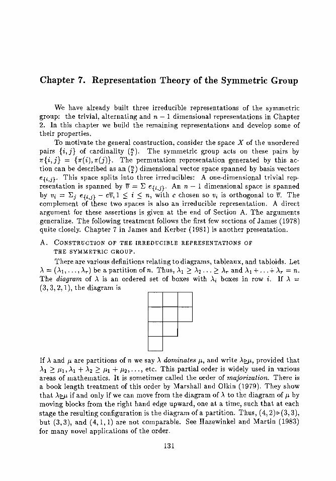
Chapter 7. Representation Theory of the Symmetric Group
We have already built three irreducible representations of the symmetricgroup: the trivial, alternating and n - 1 dimensional representations in Chapter2. In this chapter we build the remaining representations and develop some oftheir properties.
To motivate the general construction, consider the space X of the unorderedpairs {i, j} of cardinality (~). The symmetric group acts on these pairs by7r{i,j} = {7r(i),7r(j)}. The permutation representation generated by this action can be described as an (2') dimensional vector space spanned by basis vectorse{i,j}. This space splits into three irreducibles: A one-dimensional trivial representation is spanned by v = ~ e{i,j}. An n - 1 dimensional space is spannedby Vi = ~j e{i,j} - cv, 1 ~ i ~ n, with c chosen so Vi is orthogonal to v. Thecomplement of these two spaces is also an irreducible representation. A directargument for these assertions is given at the end of Section A. The argumentsgeneralize. The following treatment follows the first few sections of James (1978)quite closely. Chapter 7 in James and Kerber (1981) is another presentation.
A. CONSTRUCTION OF THE IRREDUCIBLE REPRESENTATIONS OF
THE SYMMETRIC GROUP.
There are various definitions relating to diagrams, tableaux, and tabloids. LetA == (AI, ... , Ar ) be a partition of n. Thus, Al ~ A2 ... ~ Ar and Al +...+Ar = n.The diagram of A is an ordered set of boxes with Ai boxes in row i. If A ==(3,3,2,1), the diagram is
If A and J.L are partitions of n we say A dominates J.L, and write A~, provided thatAl ~ ILl, Al + A2 ~ ILl + IL2, ... , etc. This partial order is widely used in variousareas of mathematics. It is sometimes called the order of majorization. There isa book length treatment of this order by Marshall and Olkin (1979). They showthat Af2:Jt if and only if we can move from the diagram of A to the diagram of J.l bymoving blocks from the right hand edge upward, one at a time, such that at eachstage the resulting configuration is the diagram of a partition. Thus, (4, 2) I> (3,3),but (3,3), and (4,1,1) are not comparable. See Hazewinkel and Martin (1983)for many novel applications of the order.
131
132 Chapter 7A
A A-tableau is an array of integers obtained by placing the integers from 1through n into the diagram for A. Clearly there are n! A-tableaux.
The following lemma is basic:
LEMMA O. Let A and J-L be partitions of n, suppose that tl is a A-tableau and t2is a J-L-tableau. Suppose that for each i the numbers from the ith row of t2 belongto different columns of tl. Then A~.
Proof. Since the numbers in the first row of t2 are in different columns oft1 , Al ~ J-Ll. The numbers in the second row of t2 are in distinct columns of tl,so no column of t 1 can have more than two of the numbers in the first or secondrow of t2 • Imagine "sliding these numbers up to the top of the columns of t1 ."
They fit in the first two rows, so At + A2 ~ J.Ll + J.L2. In general, no column of ttcan have more than i of the numbers from the first i rows of t2. 0
If t is a tableau, its column-stabilizer C t is the subgroup of Sn keeping the1 245
columns of t fixed. For example, when t == 3 6 7 , Ct ~ S{138} X S{26} X
8S{47} X S{5}' The notation S{i,j, ... ,k} means the subgroup of Sn permuting onlythe integers in brackets.
Define an equivalence relation on the set of A-tableaux by considering tl rv t 2if each row of tI contains the same numbers as the corresponding row of t2. Thetabloid {t} is the equivalence class of t. Think of a tabloid as a "tableau withunordered row entries." The permutations operate on the tabloids in tIle obviousway. The action is transitive and the subgroup stablizing the tabloid with 1, ... , Alin the first row, Al + 1, ... , Al + A2' in the second row, etc., is
S{I,2,... ,Al} X S{Al+I,... ,Al+A2} X ....
It follows that there are n!/AI! ... Ar ! A-tabloids.Define the permutation representation associated to the action of Sn on
tabloids as a vector space with basis e{t}. It is denoted MA. This representation is reducible but contains the irreducible representation we are after. To getthis, define for each tableau t a polytabloid et E MA by
et == L sgn( 7r )eJr"{t}.Jr"EC t
Check that 1ret == eJr"t, so the subspace of MA spanned by the {et} is invariantunder Sn (and generated as an "Sn module" by any et). It is called the Spechtmodule SA. The object of the next collection of lemmas is to prove that SA isirreducible and that all the irreducible representations of Sn arise this way. Theselemmas are all from Section 4 of James.
LEMMA 1. Let A and J-L be partitions of n. Suppose that t is a A tableau and sis a f..L-tableau. Suppose that
~ sgn(~)e~{s} # O.1rECt
Representation Theory of the Symmetric Group 133
Then Af?.Jl, and if A = p, the sum equals ±et.
Proof. Suppose for some a, b that a and b are in the same row of s and in thesame column of t. Then
(id - (ab))e{s} = e{s} - e{s} = o.
Since a and b are in the same column of t, the group < id, (ab) > is a subgroup of et. Let lTl, ••. ,lTk be coset representatives, so 2: sgn(7r)e 7r{s} =
1rECt
kE sgn(lTi)lTi{id - (ab)}e{s} = o. This is ruled out by hypothesis, so the numbersi=lin the ith row of s are in different columns of t. Lemma 0 implies that Af?.Jl.
Suppose A = J,L, and the sum does not vanish; then, again, numbers in theith row of s appear in different columns of t. It follows that for a unique 7r* ECt ,7r*{t} = {s} and this implies that the sum equals ±et (replace {s} by 7r*{t}in the sum). 0
LEMMA 2. Let J,L E MJ1., and let t be a J,L tableau. Then for some scalar c
L sgn(7r)1ru = c et·
1rECt
Proof. u is a linear combination of e{s}. For u = e{s}, Lemma 1 gives the resultwith c = 0 or ±1. 0
Now put an inner product on MJ.L which makes e{s} orthonormal: < e{s},e{t} > = 1 if {s} = {t} and 0 otherwise. This is Sn invariant. Consider the "operator" At E sgn(7r)7r. For any u,v E MJ.L, < Atu,v > =
1rECt
E sgn 7r < 1rU, V > = E sgn 7r < U,7r-1V > = < u, Atv>. Using this inner
product we get:
LEMMA 3. (Submodule Theorem). Let U be an invariant subspace of MA. Theneither U :> SA or U C SA.l. In particular, SA is irreducible.
Proof. Suppose U E U and t is a A-tableau. By Lemma 2, Atu is a constanttimes et. If we can choose u and t such that this constant is non-zero, then et E Uand, since 7ret = e1rt, SA C U. If Atu = 0 for all t and u, then 0 = < Atu, e{t} >= < u,At e{t} > = < U,et >. So U C SA.l. 0
At this stage we have one irreducible representation for each partition Aof n. The number of irreducible representations is the same as the number ofconjugacy classes: see Theorem 7 of Chapter 2. This number is also the numberof partitions of n as explained at the beginning of Chapter 2D. Hence, if \ve canshow that the SA are all inequivalent, we have finished determining all of theirreducible representations of Sn.
134 Chapter 7A
LEMMA 4. Let T: MA -7 MJ-L be a linear map that commutes with the action ofSn. Suppose that SA et ker T. Then )..~. If).. = Jl, then the restriction of T toSA is a scalar multiple of id.
Proof By lemma 3, Ker T C SAl... Thus for any t, 0 :j:. Tet = T Ate{t} = AtTe{t}.But Te{t} is a linear combination of Jl-tabloids e{s} and for at least one such e{s},At e{s} -I O. By Lemma 1, )..~. If ).. = Jl, then Tet = c et by the same argument.
o
LEMMA 5. Let T: SA --* SJ-L be a linear map that commutes with the action ofSn. 1fT -I 0, )..~.
Proof Any such T can be extended to a linear map from MA to MJ-L by definingT to be 0 on SAl... The extended map commutes with the action of Sn. If T f:. 0,then Lemma 4 implies )..~. 0
Theorem 1. The SA are all of the irreducible representations of Sn.
Proof If SA is equivalent to SJ-L, then, using Lemma 5 in both directions, ).. = Jl.o
Remark. The argument for Lemma 4 shows that the irreducible representationsin MJ-L are SJ-L (once) and some of {SA: )..~} (possibly with repeats). In fact, SAoccurs in M J-L if and only if )..~.
To complete this section, here is a direct proof of the decomposition of Mn-2,2discussed in the introductory paragraph to this chapter. We begin with a broadlyapplicable result.
A USEFUL FACT.
Let G be a finite group acting on a set X. Extend the action to the productspace X k coordinatewise. The number of fixed points of the element S E G isF( s) = I{x: sx = x }I. For any positive integer k:(1) ,b, E F(s)k = I orbits of G acting on Xkl.
s
(2) Let R, V be the permutation representation associated to X. Thus V has asbasis bx and Rs(bx ) = bsx . The character of this representation is XR(S) =F(s). If R decomposes into irreducibles as R = mlPl EB ... EB mnPn; then
~m7 = I orbits of G acting on X 2 1.
Proof. For (1) we have the action of G on X k given by S(Xl, ••• ,Xk)
(SXl, .•• ,SXk). Let Ci be a decomposition of X k into G orbits. Then
Lf(s)k = LL6sx1 (Xl) .. 'L6sxk (xk) = LL6s:f(:f)s s Xl Xk Xk s
=L L L 6S:f(:f).i fECi S
Representation Theory of the Symmetric Group 135
The innermost sum is the cardinality of the stabilizer of G at ~: INxl with N x ={s: Sf = f}. Observe N sx = S Nxs-I. In particular, the size of N x doesn'tdepend on the choice of f -in a give~ orbit. Since IQI = INxl ICil the i~ner sumequals IGI/ICil. The sum over fECi multiplies this by ICil.-The final sum yieldsIGf · IOrbitsl as required. To prove (2), we use the orthogonality of characters:XR == mIX1 + · · ·+ mnXn so < XRlxR >== mi + · · ·+ m~. On the other hand, itis clear XR(S) == F(s) and F(s-1) == F(s), so < XRlxR >== Ibl~F(s)2. 0
REMARKS AND ApPLICATIONS
(a) With k == 1, part (1) is called Burnside's lemma. It is at the heart ofSerre'sexercise 2.6 which we have found so useful. It also forms the basis of thePolya-Redfield "theory of counting." See e.g., de Bruijn (1964).
(b) If G acts doubly transitively on X, then there are two orbits of G acting onX X X:{(x,x)} and {(x,y):y:l x}. It follows that V decomposes into twoirreducible components: One of these is clearly spanned by the constants.Thus its complement {v: I;Vi == O} is irreducible.
(c) When G acts on itself we get back the decomposition of the regular representation.
(d) There is an amusing connection with probability problems. If G is considered as a probability space under the uniform distribution U, then F(s) isa "random variable" corresponding to "pick an element of G at random andcount how many fixed points it has." When G = Sn and X = {I, 2, ... , n},F(1r) is the number of fixed points of 1r. We know that this has an approximate Poisson distribution with mean 1. Part (1) gives a "formula" for allthe moments of F(g).
EXERCISE 1. Using (1), prove that the first n moments of F(1r) equal the firstn moments of Poisson(1), where 1r is chosen at random on Sn.
(e) Let us decompose Mn-2,2. The space X is the set of unordered pairs {i,j}with 1r{i,j} = {1r(i),1r(j)}. The permutation representation has dimension (2'). There are 3 orbits of Sn acting on X X X corresponding to pairs{i,j},{k,£} with 0,1, or 2 integers in common. Thus, clearly Sn acts transitively on the set of pairs ({i, j}, {i, j}). Also for ({i, j}, {j, £}) i ~ i, j andfor ({i, j}, {k, i} ) with {k, £} n {i, j} == <p. It follows that V splits into 3 irreducible subspaces. These are, the I-dimensional space spanned by v = ~e{ij},
the n - I-dimensional space spanned by Vi == ~je{ij} - cv 1 ~ i ~ n, andthe complement of these two spaces. Clearly, the space spanned by v givesthe trivial representation and the space spanned by Vi gives the n - 1 dimensional representation. What is left is n(n - 3)/2 dimensional. If \veregard the permutation representation as the set of all functions on X withsf(x) = f(s-1 x ), then the trivial and n - 1 dimensional representations arethe set of functions of form f {i, j} == i1 (i) + i1 (j).
EXERCISE 2. Show that for fixed j, 0 ~ j ~ n/2, Mn-j,j splits into j + 1distinct irreducible representations, the ith having dimension (7) - (i~1).· Hint:use the useful fact and induction, (e) above is the case j == 2.
136 Chapter 7B
We can build some new irreducible representations directly by tensoring therepresentation we know about with the alternating representation. Tensoring thealternating representation with the n - 1 dimensional representation always givesa different irreducible representation. For n = 4 we already have all irreduciblerepresentations: 2 of 1 dimension, 2 of 3 dimensions and 1 of dimension n(n 3)/2 = 2. The sum of squares adds to 24. For n >- 4 (but not n = 4) then(n - 3)/2 dimensional representation yields a new irreducible representation ofthe same dimension. For n = 5 this gives all the irreducible representations but1. We can build this by considering the action of Sn on ordered pairs (i, j). Thatis, M 3,1,1.
B. MORE ON REPRESENTATIONS OF Sn
The books by James and James-Kerber are full of interesting and useful facts.Here is a brief description of some of the most useful ones, along with pointers toother work on representations of Sn.
(1) The Standard Basis of SA. We have defined SA as the representation ofMA generated by elements et. There are n! different et and the dimension of SAcan be quite small. For example, if A = (n-1, 1), we know SA is n-1 dimensional.It turns out that a few of the et generate SA. Define t to be a standard tableau
if the numbers increase along the rows and down the columns. Thus IIIII[] is[illJa standard [3, 2] tableau. There is only 1 standard (n) tableau. There are n - 1standard (n - 1,1) tableaux. In Section 8, James proves that {etlt is a standardA-tableau} is a basis for SIL. This is a beautiful result, but not so helpful in "reallyunderstanding SA." What one wants is a set of objects on which Sn acts thatare comprehensible. The graphs in Section 5 of James are potentially very usefulin this regard for small n. As far as I know, a "concrete" determination of therepresentations of Sn is an open problem. See (6) below.
(2) The Dimension of SA. There are a number of formulas for the dimension(and other values of the character) of the representation associated to A. Thedimensions get fairly large; they are bounded by vnr of course, but they get quitelarge:
nmax dim
2 3 4 5123 6
5 7 8 9 1016 35 90 216 768
We know that dim(SA) equals the number of ways of placing the numbers 1, ... , ninto the Young diagram for A in such a way that the numbers increase along rowsand down columns. From this follows bounds like the following which was souseful in Chapter 3:
dim(SA) ~ C)J(n - AI)! ·
There is a classical determinant formula (James, Corollary 19.5)
dim(SA)= n! DetI1/(Ai - i + j)!I, where l/r! = 0 if T < o.Finally, there is the hook formula for dimensions. Let A be a partition of n. The(i, j) hook is that part of the Young diagram that starts at (i, j) and goes as far
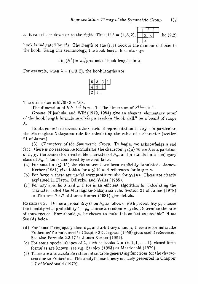
Representation Theory of the Symmetric Group 137
as it can either down or to the right. Thus, if A = (4,3, 2),~ the (2,2)
hook is indicated by x's. The length of the (i, j) hook is the number of boxes inthe hook. Using this terminology, the hook length formula says
dim(SA) = n!/product of hook lengths in A.
For example, when A = (4,3,2), the hook lengths are
653 14312 1
The dimension is 9!/6! · 3 = 168.The dimension of s(n-l,l) is n - 1. The dimension of 5 11. .. 1 is 1.Greene, Nijenhuis, and Wilf (1979, 1984) give an elegant, elementary proof
of the hook length formula involving a random "hook walk" on a board of shapeA.
Hooks come into several other parts of representation theory - in particular,the Murnaghan-Nakayama rule for calculating the value of a character (section21 of James).
(3) Characters of the Symmetric Group. To begin, we acknowledge a sadfact: there is no reasonable formula for the character XA(J-l) where A is a partitionof n, XA the associated irreducible character of Sn, and J.l stands for a conjugacyclass of Sn. This is countered by several facts.(a) For small n (~ 15) the characters have been explicitly tabulated. James
Kerber (1981) give tables for n ~ 10 and references for larger n.(b) For large n there are useful asymptotic results for XA (J-L). These are clearly
explained in Flatto, Odlyzko, and Wales (1985).(c) For any specific A and J.l there is an efficient algorithm for calculating the
character called the Murnaghan-Nakayama rule. Section 21 of James (1978)or Theorem 2.4.7 of James-Kerber (1981) give details.
EXERCISE 3. Define a probability Q on Sn as follows: with probability Pn choosethe identity with probability 1 - Pn choose a random n-cycle. Determine the rateof convergence. How should Pn be chosen to make this as fast as possible? Hint:See (d) below.
(d) For "small" conjugacy classes J.l, and arbitrary n and A, there are formulas likeFrobenius' formula used in Chapter 3D. Ingram (1950) gives useful references.See also Formula 2.3.17 in James-Kerber (1981).
(e) For some special shapes of A, such as hooks A = (k, 1,1, ... ,1), closed formformulas are known, see e.g. Stanley (1983) or Macdonald (1979).
(f) There are also available rather intractable generating functions for the characters due to Frobenius. This analytic machinery is nicely presented in Chapter1.7 of Macdonald (1979).
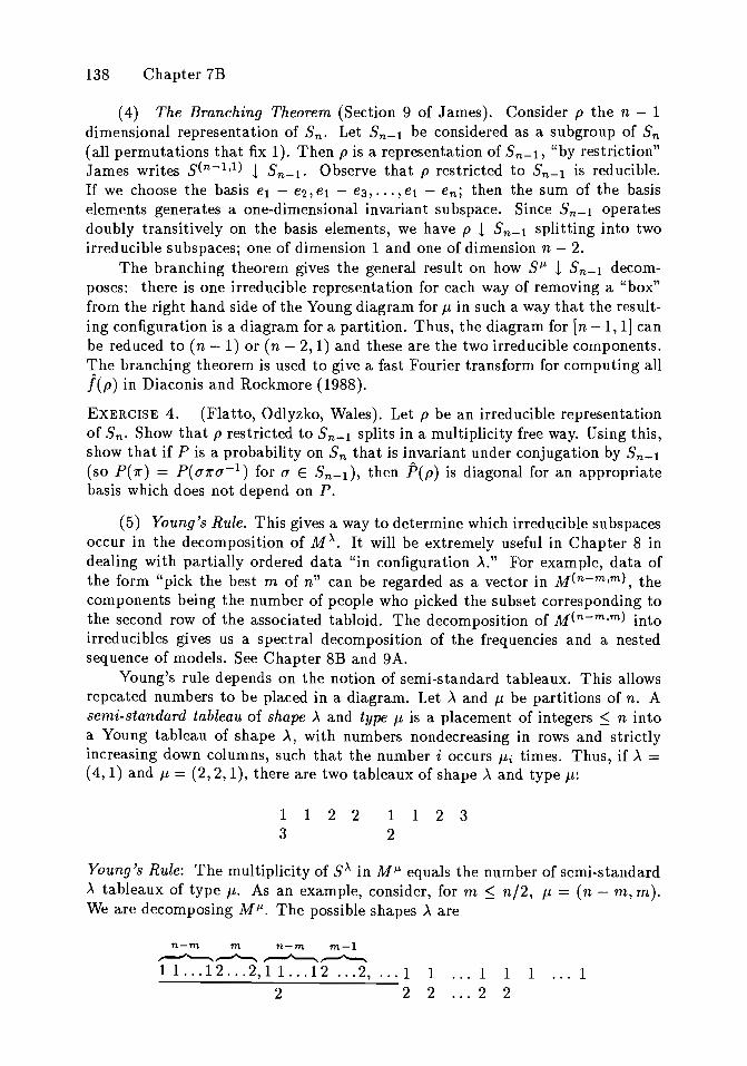
138 Chapter 7B
(4) The Branching Theorem (Section 9 of James). Consider p the n - 1dimensional representation of Sn. Let Sn-I be considered as a subgroup of Sn(all permutations that fix 1). Then p is a representation of Sn-I, "by restriction"James writes s(n-I,I) ! Sn-I. Observe that p restricted to Sn-I is reducible.If we choose the basis el - e2, el - e3, ... ,el - en; then the sum of the basiselements generates a one-dimensional invariant subspace. Since Sn-I operatesdoubly transitively on the basis elements, we have p ! Sn-I splitting into twoirreducible subspaces; one of dimension 1 and one of dimension n - 2.
The branching theorem gives the general result on how SJ.L ! Sn-I decomposes: there is one irreducible representation for each way of removing a "box"from the right hand side of the Young diagram for J1 in such a way that the resulting configuration is a diagram for a partition. Thus, the diagram for [n -1,1] canbe reduced to (n - 1) or (n - 2,1) and these are the two irreducible components.The branching theorem is used to give a fast Fourier transform for computing allj(p) in Diaconis and Rockmore (1988).
EXERCISE 4. (Flatto, Odlyzko, Wales). Let p be an irreducible representationof Sn. Show that p restricted to Sn-I splits in a multiplicity free way. Using this,show that if P is a probability on Sn that is invariant under conjugation by Sn-I(so P(1r) == P(a1ra- l
) for a E Sn-I), then Pep) is diagonal for an appropriatebasis which does not depend on P.
(5) Young's Rule. This gives a way to determine which irreducible subspacesoccur in the decomposition of M A. It will be extremely useful in Chapter 8 indealing with partially ordered data "in configuration A." For example, data ofthe form "pick the best m of n" can be regarded as a vector in M(n-m,m), thecomponents being the number of people who picked the subset corresponding tothe second row of the associated tabloid. The decomposition of M(n-m,m) intoirreducibles gives us a spectral decomposition of the frequencies and a nestedsequence of models. See Chapter 8B and 9A.
Young's rule depends on the notion of semi-standard tableaux. This allowsrepeated numbers to be placed in a diagram. Let A and J.L be partitions of n. Asemi-standard tableau of shape A and type J1 is a placement of integers ~ n intoa Young tableau of shape A, with numbers nondecreasing in rows and strictlyincreasing down columns, such that the number i occurs J-Li times. Thus, if A =(4,1) and J.L == (2, 2, 1), there are two tableaux of shape A and type J.L:
1 1223
1 1232
Young's Rule: The multiplicity of SA in MJ.L equals the number of semi-standardA tableaux of type J.L. As an example, consider, for m ~ n/2, J.L == (n - m, m).We are decomposing MJ.L. The possible shapes A are
n-m m n-m m-I~~~~
1 1 ... 1 2 ... 2, 1 1 ... 12 ... 2, ... 1 1222
1 1 1 ... 12 2
Representation Theory of the Symmetric Group 139
Each occurs once only. Thus M(n-m,m) = s(n) EB s(n-l,l) EB s(n-2,2) EB ... El)
s(n-m,m). By induction dim s(n-m,m) == (~) - (m~l). When we translate thisdecomposition into an interpretation for "best m out of n" data, the subspacess(n-m,m) have interpretations:
sn - The grand mean or # of people in sample.
sn-l,l - The effect of item i, 1 ~ i ~ n.
sn-2,2 - The effect of items {i, j} adjusted for the effect of i and j.
sn-k,k - The effect of a subset of k items adjusted for lower order effects.
Remarks. Many further examples of Young's rule appear in Chapter 8. Young'srule does not give an algorithm for decomposing MJ.£ or interpreting the SJ.£. Itjust says what pieces appear. Section 17 of James (1978) solves both of theseproblems in a computationally useful way. This remark is applied in Chapter 8Cbelow.
Young's rule is a special case of the Littlewood-Richardson rule which describes how a given representation of Sn restricts to the subgroup Sk X Sn-k. SeeJames and Kerber (1981, Sec. 2.8).
(6) Kazhdan-Lusztig Representations. The construction of the irreduciblerepresentations given in Section A constructs SA as a rather complicated subspaceof the highly interpretable MA. Even using the standard basis ((1) above), SA isspanned by the mysterious Young symmetrizers et. It is desirable to have a moreconcrete combinatorial object on which the symmetric group acts, with associatedpermutation representation isomorphic to SA. An exciting step in this directionappears in Kazhdan and Lusztig (1979). They construct graphs on which Snacts to give SA. For n ~ 6, these graphs are available in useful form. Kazhdanand Lusztig construct these representations as part of a unified study of Coxetergroups. The details involve an excursion into very high-powered homology. Garsiaand McLarnan (1988) gives as close to an "in English" discussion as is currentlyavailable, showing the connections between Kazdahn and Lusztig's representationsand Young's natural representation as developed in Chapter 3 of James-I{erber.
(7) The Robinson-Schensted-Knuth (RSK) Correspondence. There is a fascinating connection between the representation theory of Sn and a host of problemsof interest to probabilists, statisticians, and combinatorialists centered about theR-S-K correspondence. The connected problems include sweeping generalizationsof the ballot problem: if one puts At-ones, A2-twos, ..., Ak - k's into an urn anddraws without replacement, where At 2: A2 ... 2: Ak is a partition of n, then thechance that # ones 2:: # two 2:: ... 2:: # k's at each stage of the drawing equalsf(A)fn! where f(A) == dim(SA) discussed in (2) above. This links into formulas for the coverage of I{olmogorov-Smirnov tests, the distribution of the longestincreasing subsequence in a permutation, and much else.
The connection centers around a 1-1 onto map 7I" ~ (P, Q) between Sn andpairs of standard Young tableaux of the same shape. Since there are f(A) of
140 Chapter 7B
these tableaux of shape A, we have an explicit interpretation of the formula n! ='E A f(A)2.
One route to accessing this material starts with Section 5.1.4 in Knuth (1975).Then try Stanley (1971), then some of the papers in Kung (1982). Narayana(1979) gives pointers to some statistical applications. Kerov and Virshik (1985)give applications to statistical analysis of other aspects of random permutations.White (1983) discusses the connection between the R-S-I<: correspondence and theLittlewood-Richardson rule.
Chapter 8. Spectral Analysis
Often data are presented as a function f( x) defined on some index set X. IfX is connected to a group, the function f can be "Fourier expanded" and onemay try to interpret its coefficients. This is a rich idea which includes the usualspectral analysis of time series and the analysis of variance.
This chapter develops the idea in stages. First, for data on groups (timeseries, binary vectors, and permutation data). Then the idea is developed fordata on homogeneous spaces (the sphere and partially ranked data). Next sometheory needed for practical computation is derived. All of this is illustrated forsome classical designs in the analysis of variance. Finally, some research projectsare spelled out.
A. DATA ON GROUPS
1. Time series analysis. Fourier analysis of time series or other signals isa familiar scientific activity. For example, data on the number of babies borndaily in New York City over a five year period are studied by Izenman and Zabell(1978). Here X = {1, 2, ... , n} with n = 5 X 365 + 1. The data are represented asa function f( x) = # born on day x. Inspection of this data shows strong periodicphenomena: about 450 babies are born on each week day and about 350 on eachday of the weekend. (Physicians don't like to work on weekends.) There mightalso be monthly or quarterly effects.
To examine (and discover) such phenomena, scientists pass from the originaldata f(x) to its Fourier transform
j(y) = ~xf(x) e2trixy/n
where the sum runs over x == 0, 1, ... , n - 1. Fourier inversion gives
It sometimes happens that a few values of j(y) are much larger than therest and determine f in the sense that f is closely approximated by the functiondefined by using only the large Fourier coefficients in the inversion formula. Whenthis happens, we have f approximated by a few simple periodic functions of x,e.g. e-2trixy/n, and may feel we understand the situation.
The hunting and interpretation of periodicities is one use of spectral analysis.A splendid introduction to this subject is given by Bloomfield (1976). A moreadvanced treatment from the same point of view is given by Brillinger (1975).
141
142 Chapter 8A
There are other interpretations of spectral analysis. The discussion papersby Jenkins (1961) and Parzen (1961) present a useful survey of different views.Some further discussion is given in the last section of this chapter. For now, wewill stick to the data analytic view outlined above.
2. Permutation data. Spectral analysis can be carried out for any group usingthe matrix entries of the irreducible representations as a basis. Before developingthis in general, here is an example.
In Chapter 5-A we discussed rankings of three items. People were asked torank where they wanted to live: in a city, suburbs, or country. The rankings were
1r city suburbs country #id 1 2 3 242(23) 1 3 2 28(12) 2 1 3 170
(132) 3 1 2 628(123) 2 3 1 12
(13) 3 2 1 359
Here X = S3, and f(1r) is the number choosing 1r. There are three irreduciblerepresentations of S3: the trivial, sgn, and two-dimensional representation p. TheFourier inversion theorem gives
f(1r) = ~{j(triv) + sgn(1r)' j(sgn) +2Tr(p(1r-1 )j(p)).
Expanding the trace gives a spectral analysis of f as a sum of orthogonal functions.To facilitate comparison between functions in this basis, let us choose an
orthogonal version of p. Thus, using cycle notation on S3
tr id (1 2) (2 3) (1 3) (1 2 3) (1 3 2)
p(tr) (01 °1) (-01 °1) 1 (1 V3) 1 (1 -V3) 1 (-1 -V3) 1 (-1 V3)2" V3 -1 2" -V3 -1 2 V3 -1 2" -V3 -1
These are arrived at by choosing Wl = 1(e1 - e2), W2 = ~(el +e2 - 2e3)
as an orthonormal basis for {v E R3: VI + V2 + V3 = O}. The matrices p(1r) give
the action of 1r in this basis. Now
j(triv) = 1439, j(sgn) = 242 - 28 - 170 +628 + 12 - 359 = 325,
A _ (-54.5 285v'3/2)f(p) - -947v'3/2 -101.5 ·
Define four functions on S3 by
Spectral Analysis 143
With this definition, the functions 1, sgn 1r, a(1r), b(1r), c(1r), d(1r) are orthogonaland have the same length.
Expanding the trace in the Fourier inversion theorem gives
1f(rr) = 6"{1439 +325 sgn(rr) - 54.5V2 a(rr) - 947V3fi b(rr) +285-../3/2 c(rr)
- 101.5V2 d(1r)}.
== ~{1439 +325 sgn(rr) - 77 a(rr) - 1160 b(rr) +349 c(rr) - 144 d(rr)}.
As a check, when 1r = id, this becomes
242 = ~{1439 +325 - 109 - 203}.
The largest non-constant coefficient, 1160, multiplies b(1("). This is the function
1r id (1 2) (2 3) (1 3) (123) (132)b(1r) 0 0 J372 -J372 J372 -J372
or-J372 if cities are ranked 3rd (1r(1) = 3)
b(1r) = 0 if country is ranked 3rd (1r(3) = 3)
J372 if suburbs are ranked 3rd (1r(2) = 3).
Spectral analysis gives fresh insight into this little data set: After the constant, the best single predictor of f is what people rank last. Now b(1r) enterswith a negative coefficient. It "follows" that people "hate" the city most, thesuburbs least and the country in between. Going back to the data #{1r(1) = 3} =981, #{1T"(2) = 3} = 40, #{1T"(3) = 3} = 412, so the effect is real. It seems atvariance with the unfolding hypothesis, but is in fact necessary. If people makeindividual rankings by unfolding, the proportions connected to extreme ranks willbe monotone with the unfolding point in the center.
The kind of data analytic interpretation given in the last paragraph seemsmandatory - we must seek subject matter interpretation of our findings. As aword of warning, almost any set of summary statistics can have a story wovenabout them - we are good at making up stories.
EXERCISE 1. Carry out the analysis of this section for the non-orthogonalrepresentation of Sa given in Chapter 2-A. Show that the main conclusions do notchange.
3. A general case, with inference. For G a finite group, and f a function onG, the Fourier inversion theorem gives
1 -1 "f(s) = iGfEp dp Tr(p(s )f(p»·
144 Chapter 8A
Now let P be a unitary representation, so p(t)* == p(t- 1). Corollaries 2 and 3
to Schurs lemma of Chapter 2 yield orthogonality relations for the matrix entries ofp. Define the usual inner product on all functions on G: < <PI1/; > == IblE <p( t)1/;( t)*.Then
< Pijl17ki > = 0 if p and 17 are inequivalent unitary representations, for any
ij, kf.
{0 unless i == k and j = f,
< Pijlpkl > = Jp if i = k, j = f.
It follows that the functions Pij(8) = JfI; Pij(8-1 ) are orthonormal on G withrespect to < ·1· >.
To numerically compute the spectral representation, compute J(p) and expand the trace giving
l(s) = I~I ~..;;r; j(p)ji Pij{S).P,?',]
The squared length of the projection indexed by functions associated to P isdp Tr(j(p)j(p)*) == dp llj(p)11 2
•
Elementary inference. In carrying out spectral analysis, it is natural to wonder "if the data had come out a bit different, would the inferences change?" Thisis susceptible to a wealth of interpretations - from an elementary sensitivity analysis, through a bootstrap analysis, through a frequentist model through a Bayesiananalysis. At present, very little is available in off the shelf tools. We here developthe obvious normal theory. Some more speculative suggestions are contained inthe final section of this chapter.
Let G be a finite group. Suppose that an observed function f( 8) can beregarded as a true function J.L( s) plus an error or perturbation function £( s)
f( s) = J.L( s) + £(s).
The strongest possible assumptions that can be made are J.L(s) fixed (or known)and e(s) rv N(O,0-2 ) (normal, with mean 0 and variance 0-2 independent for each8). Then for an orthogonal representation p, the coefficients j(p)ijJfI; are all
independent normals, with mean JfI;~(P)ij and variance a 2 JGI. (I have assumedthat all of the representations are real. For unitary representations, complexnormal distributions occur). Further, for P and 17 inequivalent representations,j(p)ij and j(17)ki are independent.
EXERCISE 2. Prove the results in the last paragraph.If (72 is assumed known, or {1(p) == 0 is assumed for some irreducible so
(72 can be estimated, all of the usual inferential tools associated to the generallinear model are available. In particular, dp llj(p)11 2 is distributed as (12 times
Spectral Analysis 145
a chi-squared variable on d~ degrees of freedom (if jl(p) = 0). Fisher's test forthe significance of the largest Fourier coefficient (see e.g. Bloomfield (1976) orAnderson (1971)) is easily adapted to this setting.
If (J'2 is assumed to depend on s, a rich array of tools from variance components and classical multivariate analysis are available. Work of the Danish schoolis particularly relevant - see Perlman (1988) for entry into this literature.
The normality of the Fourier transforms is approximately true under muchless restrictive assumptions than normality of I( s). After all, j(p)ij is an averageof a lot of things, and will be approximately normal and independent of othercoefficients under fairly mild assumptions. This deserves to be worked out morecarefully. Anderson (1971, Sec. 2.6), Freedman and Lane (1980), or Diaconis andFreedman (1984) are useful places to start.
This seems like a good place to point out
Elementary fact. Let P be an irreducible unitary representation of G. LetL(G) be all functions on G. Consider the subspace L j spanned by the matrixentries of the jth column of p. Then L j is an invariant subspace isomorphic to p.
Proof. Let s Pij(t) = Pij(s-lt). The matrix equation p(s-l )p(t) == p(s-lt) showsthat Pij(S-lt) == Ek akPkj(t) as a function of t. Thus L j is an invariant subspace.Choosing the functions Pij, 1 ~ i ~ dp as a basis gives p(s) being the associatedmatrix representation. 0
Remarks. As j varies, the representations L j give the dp copies of p that appearin the decomposition of the regular representation. In applications, the columnsof p sometimes have a natural meaning. For example, on Sn the jth column ofthe n - I-dimensional representation codes which i is mapped to position j inone choice of basis. Expanding the trace preserves this interpretation. Furtherdiscussion of interpretability of the basis functions appears in the last section ofthis chapter.
4. Bahadur's item analysis. Bahadur (1961) introduced a spectral analysiswhen X == Zf consists of data on binary k-tuples. For example, fix k at 5 andconsider a population of families with five children. Take f( x) as the proportionof families whose children were born in birth order x - so if x == 01010, the birthorder was girl, boy, girl, boy, girl. Klotz (1970) gives an analysis of such data.
Economics has massive amounts of "panel study data." Here k might be 12and x might represent the pattern of employed/unemployed behavior for a personin the study. It is not uncommon to have samples larger than 5,000 people. Hsiao(1986) is a recent book on this subject.
Bahadur's original motivation was test score analysis, where x records thepattern of correct/incorrect guesses, and f( x) records the proportion of studentsanswering in a given pattern.
Let Xi, 1 :s; i ~ k be the coordinate projection from Z;. Let f(x) be aprobability on Zf. Define (li == Ef(Xi) and Zi == (Xi - (li)/VO!i(l- O!i). Define
146 Chapter 8A
Tij==Ef(ZiZj), i<j
Tiji == Ef(ZiZjZi), i < j < (,
Tl. .. k == E f (Zt Z2 ••• Zk).
The (~) parameters Tij are correlations. The Tiji can be thought of higher ordercorrelations, etc. Bahadur wrote the spectral decomposition of f as follows.
PROPOSITION 1. (Bahadur). For 1 a probability on Z~,
1==11 ·12
where
11 (x) = IT aft (1 - ai)1-x, is the product distribution with
margins matching f.
h(x) = 1 +L rijZiZj + L rijtZiZjZt +... + rl...kZl .. . Zk·
i<i i<i<i
Proof. Consider the vector space of all functions on Z~ with inner product< 9, h >= Efl(9· h). The set
consists of orthonormal functions: 11911 == 1 for 9 E Sand < 9, h >= 0 for 9, h E Sbut 9 :P h. There are 2k functions in S, so they form a basis. Now, set /2 == ///1.Then < 12, 9 >== ~12glt = Ef(g)· Also Ef(l) == 1, Ef(Zi) = 0, so the propositionfollows. 0
The function /2 measures departure from independence. It is natural to lookat the individual coefficients to try to understand the nature of the dependence.Let 6[k) == 1112 - 111 2
• Thus define
6{k) =L r~j + L r~jt + ···+ rLki<i i<i<i
d {'2 2=u2 + ... + Ok·
The ratios 6;/6[k) provide an index of the relative importance of the jth orderterms. Similarly, If Im is the approximation to 1 in which all terms in 12 involvinga product of more than m Zi'S are omitted, then
provides an index of quality for the approximation of I by Im.
Spectral Analysis 147
The analysis above is just the standard spectral analysis shifted to a morenatural base measure (matched marginals versus uniform). As Bahadur remarks,it is also natural to expand and analyze log f. This gets away from the problemsof interpreting negative coefficients and links into the usual log-linear analysis ofsuch data as a 2 X 2 X ... X 2 contingency table.
B. DATA ON HOMOGENEOUS SPACE
A natural and useful extension of spectral analysis occurs for homogeneousspaces. These were defined and illustrated in Chapter 3F.
1. Definitions. Let X be a finite set. Let G act transitively on X with Nthe isotropy subgroup: N == {s E G: sXo == xo} where Xo is some fixed point inX. Let L(X) be all functions from X into the complex numbers C. Then L(X)decomposes into irreducibles as
Vo ffi VI ffi · · · ffi Vk •
Suppose we are given f(x) E L(X), regarded as data - f(x) is the number (orproportion) of people having property x.
Spectral analysis is the decomposition of f( x) into its projections on theirreducible invariant subspaces of L(X), and the approximation of f(x) by assmall a number of projections as give a reasonable fit.
Here L(X) is regarded as an inner product space using < fig > ==fxr~f(x)g(x)*, and projections are orthogonal. Of course we usually want evenmore: the coefficients of f projected into Vi in some natural or interpretable basishelp connect the analysis to the original subject matter.
As shown in Corollary 1 of Section 3 below the decomposition of the regularrepresentation falls into this domain. The following are less standard.
Example 2. Partially ranked data. Let A be a partition of n. Consider dataconsisting of partial rankings of n items of shape A: thus people rank their favoriteAl items (but not within) and their next A2 items (but not within) and their finalAk items (but not within). Here n == Al +A2 +... + Ak and we do not assume Aiare ordered. Chapter 5B gives examples.
If SAl X S)..2 X •.• X S)..1e denotes the subgroup of Sn which allows permutationsamong the first Al coordinates, the next A2 coordinates, and so on, then X =Sn/S)..l X .•• X S)..Ie. The space L(X) can be taken as all real valued functions onX because all irreducible representations are real. Thus L(X) == M oX of Chapter7. The decomposition of L(X) is given by Young's rule (see Chapter 7-B). Hereare some special cases.
Case 1. A = (n - 1,1). This is simple choice data, people choosing one out ofn items. The set X may be regarded as {I, 2, ... , n} and f(x) is the number ofpeople choosing x. The decomposition is
L(X) == sn EB sn-I,l
with sn the trivial representation and sn-l,l the n-1 dimensional representation.This amounts to f(i) =7+ (f(i) -I) with 7 == *L;f(i).
148 Chapter 8B
Case 2. A = (n-2, 1, 1). Here people pick their favorite and second favorite itemsfrom a list of n (order matters). The space X may be regarded as {(i,j), 1 ~ i =Ij ~ n} so IXI = n(n - 1). The decomposition of L(X) is
L(X) == sn E9 2Sn - I ,1 E9 sn-2,2 E9 sn-2,1,1
dim n(n - 1) 1 2(n - 1) n(n - 3)/2 (n - l)(n - 2)/2.
o23
o23
To derive this, start with A = (n - 2,1,1). Consider n - 2 ones, one two, andone three. Young's rule asks for the number of ways of arranging these symbolsinto arrays which are increasing along rows, and strictly increasing down columns.The only ways are
0 23
where the block indicates n-2 ones. The number of times each shape appears givesthe multiplicity of the corresponding irreducible. The dimensions are computedfrom the hook length formula of Chapter 7.
Here there is a natural interpretation of the decomposition. The projectioninto sn represents the best constant approximation to f, Le. I = n(Ll) Ef( i, j).The two sn-l,l spaces give the effect of the first coordinate and the second coordinate respectively. The projection of j into sn E9 2Sn - I ,1 gives the best approximation to f of the form
The projection into sn-2,2 can be thought of as the best approximation of j,orthogonal to sn E9 2Sn - 1 ,1, of form
the brackets indicating unordered pairs. The projection onto sn-2,1,1 can bethought of as a residual, or what's left when the first four terms are subtractedoff.
EXERCISE 3. Verify the decompositionM n - 3,l,l,l = sn EB 3S n - 1,l EB 3S n - 2 ,2 EB sn-3,3 El) 2S n - 3 ,2,l EB 3S n - 2,l,l EB sn-3,l,l,l
n(n - 1)(n - 2) 3(n _ 1) 3n C;-3) nCn-lJCn-S) 2n Cn-;)Cn-4) 3(n;-1) (n;-l)
Can you give an interpretation to the subspaces involved?
3. Computing projections. We turn now to the problem of actually computingthe projections, choosing bases, and so on.
Method 1 - Character Theory. Let G be a group, p: G ~ GL(V) a representation.The decomposition of V into irreducibles usually requires choosing a basis. Thereis a coarser direct sum decomposition that is basis free. Let Xl, X2, . · . ,Xh bethe distinct characters of the irreducible representations W1 , •.• , Wh of G. Let
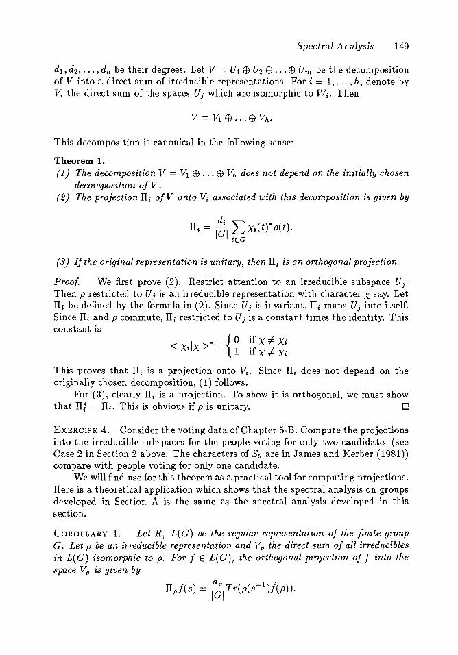
Spectral Analysis 149
d1 , d2 , • •• , dh be their degrees. Let V == U1 El) U2 EI) ••• El) Urn be the decompositionof V into a direct sum of irreducible representations. For i = 1, ... , h, denote byVi the direct sum of the spaces Uj which are isomorphic to Wi . Then
v == Vi El) • • • El) Vh .
This decomposition is canonical in the following sense:
Theorem 1.(1) The decomposition V == VI El) ••• El) Vh does not depend on the initially chosen
decomposition of V.(2) The projection Il i olV onto Vi associated with this decomposition is given by
lli = I~I E Xi(t)*p(t).tEG
(3) If the original representation is unitary, then Ili is an orthogonal projection.
Proof. We first prove (2). Restrict attention to an irreducible subspace Uj •
Then p restricted to Uj is an irreducible representation with character X say. LetIIi be defined by the formula in (2). Since Uj is invariant, Il i maps Uj into itself.Since Il i and p commute, Ili restricted to Uj is a constant times the identity. Thisconstant is
{0 if X -t x·< Xi Ix >* == ." t1 IfX#Xi.
This proves that Il i is a projection onto Vi. Since ITi does not depend on theoriginally chosen decomposition, (1) follows.
For (3), clearly IT i is a projection. To show it is orthogonal, we must showthat IT; == Il i . This is obvious if p is unitary. 0
EXERCISE 4. Consider the voting data of Chapter 5-B. Compute the projectionsinto the irreducible subspaces for the people voting for only two candidates (seeCase 2 in Section 2 above. The characters of Ss are in James and Kerber (1981))compare with people voting for only one candidate.
We will find use for this theorem as a practical tool for computing projections.Here is a theoretical application which shows that the spectral analysis on groupsdeveloped in Section A is the same as the spectral analysis developed in thissection.
COROLLARY 1. Let R, L(G) be the regular representation of the finite groupG. Let p be an irreducible representation and Vp the direct sum of all irreduciblesin L(G) isomorphic to p. For f E L(G), the orthogonal projection of f into thespace Vp is given by
dp -1 ,.llpf(s) = fGiTr(p(s )f(p»·
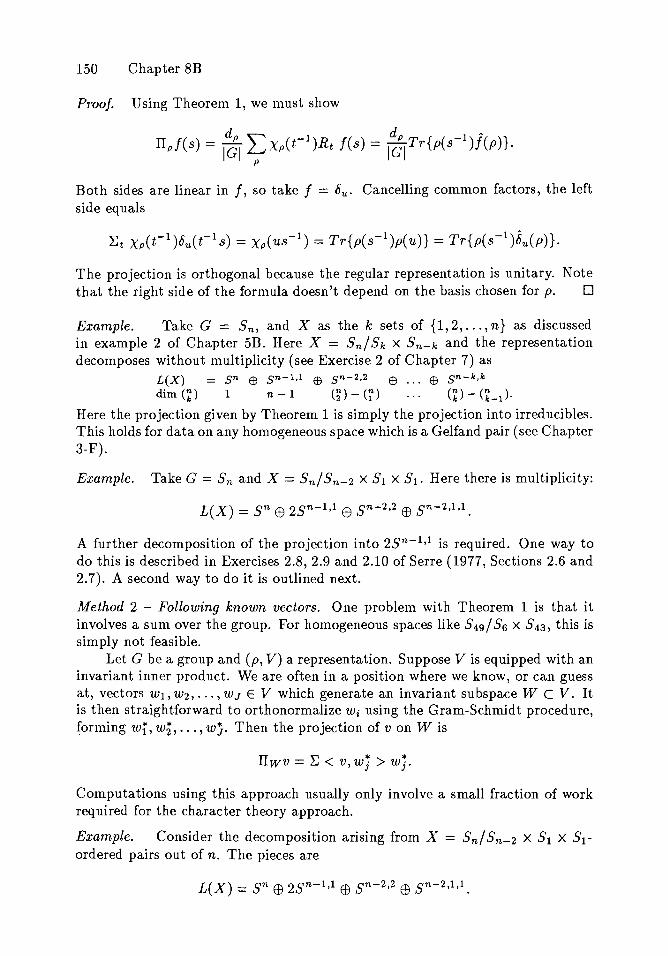
150 Chapter 8B
Proof. Using Theorem 1, we must show
TIp/(S) = I~I LXp(C1)Rt /(s) = 1~ITr{p(s-l)j(p)}.p
Both sides are linear in j, so take j == 8u . Cancelling common factors, the leftside equals
The projection is orthogonal because the regular representation is unitary. Notethat the right side of the formula doesn't depend on the basis chosen for p. 0
Example. Take G == Sn, and X as the k sets of {1,2, .. . ,n} as discussedin example 2 of Chapter 5B. Here X == Sn/ Sk X Sn-k and the representationdecomposes without multiplicity (see Exercise 2 of Chapter 7) as
L(X) = sn EB sn-1,1 EB sn-2,2 EB ... EB sn-k,k
dim (k) 1 n - 1 (2) - (1) (k) - (k -1 ).
Here the projection given by Theorem 1 is simply the projection into irreducibles.This holds for data on any homogeneous space which is a Gelfand pair (see Chapter3-F).
Example. Take G == Sn and X == Sn/ Sn-2 X SI X SI. Here there is multiplicity:
L(X) == sn EB 2Sn - l ,1 EB sn-2,2 EB sn-2,1,1.
A further decomposition of the projection into 2Sn - l ,1 is required. One way todo this is described in Exercises 2.8,2.9 and 2.10 of Serre (1977, Sections 2.6 and2.7). A second way to do it is outlined next.
Method 2 - Following known vectors. One problem with Theorem 1 is that itinvolves a sum over the group. For homogeneous spaces like S49/ S6 X S43, this issimply not feasible.
Let G be a group and (p, V) a representation. Suppose V is equipped with aninvariant i~ner product. We are often in a position where we know, or can guessat, vectors Wl, W2, .•• , W J E V which generate an invariant subspace W CV. Itis then straightforward to orthonormalize Wi using the Gram-Schmidt procedure,forming wi, w2' ... ,wj. Then the projection of v on W is
IIwv == ~ < v,wj > wj.
Computations using this approach usually only involve a small fraction of workrequired for the character theory approach.
Example. Consider the decomposition arising from X = Sn/Sn-2 X SI X Sl-ordered pairs out of n. The pieces are
L(X) == sn EB 2Sn - 1,1 EB sn-2,2 Ea sn-2,1,1.
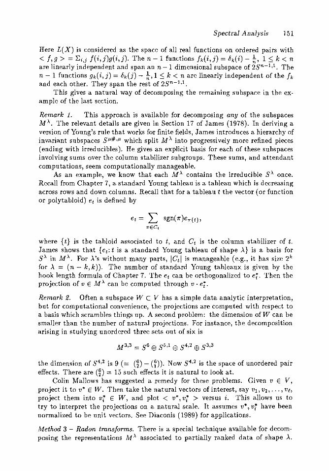
Spectral Analysis 151
Here L(X) is considered as the space of all real functions on ordered pairs with< I,g > = Ei,j f(i,j)g(i,j). The n - 1 functions fk(i,j) = 6k(i) - ~, 1 ~ k < nare linearly independent and span an n - 1 dimensional subspace of 2Sn - 1 ,1. Then - 1 functions gk(i,j) = Ok(j) - ~,1 ~ k < n are linearly independent of the Ikand each other. They span the rest of 2Sn - 1 ,1.
This gives a natural way of decomposing the remaining subspace in the example of the last section.
Remark 1. This approach is available for decomposing any of the subspacesMA. The relevant details are given in Section 17 of James (1978). In deriving aversion of Young's rule that works for finite fields, James introduces a hierarchy ofinvariant subspaces SP,#,p, which split MA into progressively more refined pieces(ending with irreducibles). He gives an explicit basis for each of these subspacesinvolving sums over the column stabilizer subgroups. These sums, and attendantcomputations, seem computationally manageable.
As an example, we know that each MA contains the irreducible SA once.Recall from Chapter 7, a standard Young tableau is a tableau which is decreasingacross rows and down columns. Recall that for a tableau t the vector (or functionor polytabloid) et is defined by
et = L sgn(rr)e1r{t},
1rECt
where {t} is the tabloid associated to t, and Ct is the column stabilizer of t.James shows that {et: t is a standard Young tableau of shape A} is a basis forSA in MA. For A's without many parts, ICtl is manageable (e.g., it has size 2k
for A = (n - k, k». The number of standard Young tableaux is given by thehook length formula of Chapter 7. The et can be orthogonalized to e;. Then theprojection of v E MA can be computed through v · e;.
Remark 2. Often a subspace W C V has a simple data analytic interpretation,but for computational convenience, the projections are computed with respect toa basis which scrambles things up. A second problem: the dimension of W can besmaller than the number of natural projections. For instance, the decompositionarising in studying unordered three sets out of six is
the dimension of 8 4 ,2 is 9 (= (~) - (~». Now 84 ,2 is the space of unordered paireffects. There are (~) = 15 such effects it is natural to look at.
Colin Mallows has suggested a remedy for these problems. Given v E V,project it to v* E W. Then take the natural vectors of interest, say Vt, V2, . .. , Vi,
project them into vi E W, and plot < v*, vi > versus i. This allows us totry to interpret the projections on a natural scale. It assumes v*, vi have beennormalized to be unit vectors. See Diaconis (1989) for applications.
Method 3 - Radon transforms. There is a special technique available for decomposing the representations MA associated to partially ranked data of shape A.
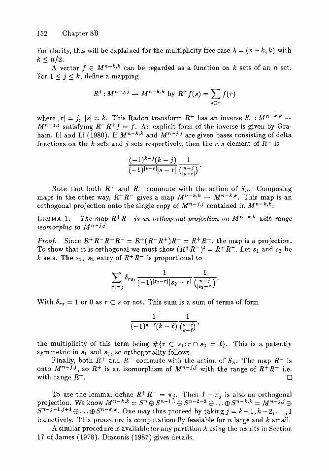
152 Chapter 8B
For clarity, this will be explained for the multiplicity free case A = (n - k, k) withk ~ n/2.
A vector f E Mn-k,k can be regarded as a function on k sets of an n set.For 1 ~ j ~ k, define a mapping
R+: Mn-j,j --t Mn-k,k by R+ f(s) =L fer)s:)r
where Irl = j, Isl = k. This Radon transform R+ has an inverse R-: Mn-k,k ~
Mn-j,j satisfying R- R+ f = f. An explicit form of the inverse is given by Graham, Li and Li (1980). If Mn-k,k and Mn-j,j are given bases consisting of deltafunctions on the k sets and j sets respectively, then the r,8 element of R- is
(-l)k- j (k - j) 1
(-l)ls-r'ls - rl (n- j )·Is-rl
Note that both R+ and R- commute with the action of Sn. Composingmaps in the other way, R+ R- gives a map Mn-k,k ~ Mn-k,k. This map is anorthogonal projection onto the single copy of Mn-j,j contained in Mn-k,k:
LEMMA 1. The map R+ R- is an orthogonal projection on Mn-k,k with rangeisomorphic to Mn- j,j .
Proof. Since R+ R- R+ R- = R+(R- R+)R- = R+ R-, the map is a projection.To show that it is orthogonal we must show (R+ R-)t = R+ R-. Let 81 and 82 bek sets. The SI, 82 entry of R+ R- is proportional to
With 6rs = 1 or 0 as r C 8 or not. This sum is a sum of terms of form
1 1(-l)k-i(k - f) (n- j ) ,k-i
the multiplicity of this term being #{r C 81: r n 82 = f}. This is a patentlysymmetric in 81 and 82, so orthogonality follows.
Finally, both R+ and R- commute with the action of Sn. The map R- isonto Mn-j,j, so R+ is an isomorphism of Mn-j,j with the range of R+ R- Le.with range R+. 0
To use the lemma, define R+ R- = 'Trj. Then I - 'Trj is also an orthogonalprojection. We know Mn-k,k = sn EB sn-l,1 EB sn-2-2 EB ... EB sn-k,k = Mn-j,j EBsn-j-l,i+1 E9 ... EB sn-k,k. One may thus proceed by taking j = k - 1, k - 2, ... , 1inductively. This procedure is computationally feasiable for n large and k small.
A similar procedure is available for any partition A using the results in Section17 of James (1978). Diaconis (1987) gives details.
Spectral Analysis 153
Final remarks on choice of basis. Return to data f on a group G. The Fouriertransform j(p) can be a completely arbitrary matrix for general f. To see this,just define f by the inversion theorem to have a prescribed j(p). There is arather complex restriction, akin to Bochner's theorem but more complex, when fis positive. For practical purposes J(p) is an essentially arbitrary matrix.
We have available the possibility of changing bases, changing from J(p) toA J(p)A -1. As A varies, the invariants of J(p) are its eigenvalues, or its "canonicalform."
To compare coefficients within j(p) and between various p's, it seems naturalto consider only unitary (or orthogonal) base changes. Then, there is not muchthat can be done to bring J(p) into a simple form. One possibility is to rotate tomake the first few rows of j as large as possible.
Other possibilities are to change bases to bring the matrix into a simpleform. For example, any matrix can be conjugated by an orthogonal matrix to thesum of a diagonal and skew symmetric matrix: A = teA + At) + teA - At), andA + At = rDrt , so rArt = tD + S, with D diagonal and S skew symmetric.Any matrix can be orthogonally conjugated to lower triangular form (essentially)see Golub and van Loane (1983).
The choice of bases must balance off
• computational convenience
• ease of interpretation
• convenience of orthogonality
• maximal informativeness of a few projections
• invariance considerations.
Nobody ever said statistics was easy.
At present, we can have the first three properties, for partially ranked data,by using methods 2 or 3 and Mallows' idea as outlined under method 2. There isplenty to think about.
c. ANALYSIS OF VARIANCE.
Analysis of variance (ANOVA) is a set of techniques for analyzing cross tabulated data such as two-way arrays. Data analytically, ANOVA is a special case ofspectral analysis as described in Section B. This section develops the connection,and explains a technique introduced by Peter Fortini for defining the group forthe array from a naturally given set of factors.
There is more to ANOVA than the data analytic aspects presented here.Section D-4 describes some of the other ideas. Hopefully they can be developedfor other types of spectral analysis.
1. Classical examples.
Example 1. Two-way ANOVA with 1 repetition per cell. Here data are collectedin a two way layout
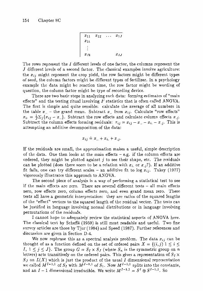
154 Chapter SC
X11 X12 • .. X1J
X21
Xl1 XIJ
The rows represent the I different levels of one factor, the columns represent theJ different levels of a second factor. The classical examples involve agriculture:the Xij might represent the crop yield, the row factors might be different typesof seed, the column factors might be different types of fertilizer. In a psychologyexample the data might be reaction time, the row factor might be wording ofquestion, the column factor might be type of recording device.
There are two basic steps in analyzing such data: forming estimates of "maineffects" and the testing ritual involving F statistics that is often called ANOVA.The first is simple and quite sensible: calculate the average of all numbers inthe table x .. - the grand mean. Subtract x .. from Xij. Calculate "row effects"Xi. == t~j{Xii - X .. }. Subtract the row effects and calculate column effects x.j.
Subtract the column effects forming residuals: Tij == Xij - X .. - Xi. - x.j' This isattempting an additive decomposition of the data:
Xii == x .. + Xi. + x.i·
If the residuals are small, the approximation makes a useful, simple descriptionof the data. One then looks at the main effects - e.g. if the column effects areordered, they might be plotted against j to see their shape, etc. The residualscan be plotted (does there seem to be a relation with XiI or Xlj?). If an additive·fit fails, one can try different scales - an additive fit to log Xij' Tukey (1977)vigorously illustrates this approach to ANOVA.
The second piece of analysis is a way of performing a statistical test to seeif the main effects are zero. There are several different tests - all main effectszero, row effects zero, column effects zero, and even grand mean zero. Thesetests all have a geometric interpretation: they are ratios of the squared lengthsof the "effect" vectors to the squared length of the residual vector. The tests canbe justified in language involving normal distributions or in language involvingpermutations of the residuals.
I cannot hope to adequately review the statistical aspects of ANOVA here.The classical text by Scheffe (1959) is still most readable and useful. Two finesurvey articles are those by Tjur (1984) and Speed (19S7). Further references anddiscussion are given in Section D-4.
We now rephrase this as a spectral analysis problem. The data Xij can bethought of as a function defined on the set of ordered pairs X == {(i, j) 1 ::; i ~I, 1 ::; j ::; J}. The group G == SI X SJ (where Sn is the symmetric group on nletters) acts transitively on the ordered pairs. This gives a representation of SIXSJ on L(X) which is just the product of the usual I dimensional representationwe called MI-1,1 of SI with M J -1,1 of Sl. Now MI-1,1 splits into the constants,and an I-I dimensional irreducible. We write M I - 1 ,1 == SI EB SI-1,1. So
Spectral Analysis 155
M 1- 1 ® MJ-1=(SI EB SI-l,l)®(SJ EB SJ-l,1)=TrivEBS1-1,1 ® TrivEBSJ-1,1 ® TrivEBS1-1,1 ® SJ-l,l
dim IxJ 1 I-I J-l (/-l)(J-l)
The observed array Xij is just a vector in L(X). The projection of x into theinvariant irreducible subspaces gives the usual ANOVA decompositon: the projection onto the one dimensional space of constants is the array with constantentry x ... The projection onto SI-1,1® triv is onto all arrays which are constantin each row, with the constants summing to zero. These constants are Xi. Thefinal space is spanned by the residuals Tij.
The lengths of these projections give the usual sums of squares required forthe classical ANOVA table. The dimensions of the various irreducible subspacesgive the degrees of freedom for the classical F tests.
Example 2. Two way ANOVA with repeated entries - wreath products. In thisexample, data are collected in a two way array, but k observations are collectedat each level of the two factors. It is intuitively clear that the appropriate groupof symmetries allows permutations of rows and columns and, within each row andcolumn, an arbitrary permutation of the k elements in that cell among each other.To write this down neatly, it is useful to introduce the notion of wreath product.
Let G be any group and H a subgroup of Sn. Define a group G wr H asfollows. The group consists of the set of elements in Gn XH == {(91, 92, ... , 9n; h)}.The product of two elements is
(91, · · ., 9n; h)(g~, · · ., 9~; h') = (glg~-1(1)' · · ., gng~-l(n); hh').
Th ·d t·t · ( . .. ) ( h)-l (-1 -1 h- 1 )e 1 en 1 y IS 'tG,···,'tG; 'tH, gl,···,9n; = gh- 1(1), ... ,9h-1(n); .The subgroup Gn sits in G wr H as a normal subgroup. H sits in G wr H as{(iG , ... ,iG ; h)}. G wr H is the semi-direct product ofGn and H.
For an I X J table with k replications per cell, the natural symmetry groupis Sk wr(SI X SJ). The representation theory of wreath products is completelyknown in terms of the irreducible representations of G and H. A reasonabletreatment is Chapter 4 of James and Kerber (1981). When this theory is appliedto ANOVA there are no surprises; the decomposition is the one derived in allstandard texts; see Example 4 below for a special case.
Example 3. The Diallel Cross Design. This design is used by animal or plantbreeders to find new hybrid species of known species. Consider n known typesof plant. Form all (~) crosses of distinct strains. The data are some measurablecharacteristic of each offspring (yield, size, etc.). Here the data are indexed byunordered pairs {i,j}. The natural symmetry group is Sn; the standard ANOVAdecomposition corresponds to the decomposition of what we have called Mn-2,2 ~
sn EB sn-1,1 EB sn-2,2.
We will return to examples after a general definition of the symmetry groupof a designed experiment.
2. A systematic approach. In the examples above we just wrote down a groupand showed how spectral analysis gave "the usual" ANOVA.
Alan James (1957,1982) and Ted Hannan (1965) introduced ideas to relate analgebraic object to a designed experiment. Gleason and McGilchrist (1978) give
156 Chapter 8C
a more detailed account of these ideas. Lederman (1967) independently pointedout the connection between ANOVA and representation theory.
Peter Fortini (1977) extended these ideas to give a reasonably systematictheory. His work associates a group in a natural way to an experiment given interms of classical factors. Then spectral analysis can be used as before. Here is abrief account of Fortini's ideas.
Let X be a finite set. We will work with observations indexed by X.
Definition 1. A factor f of the design indexed by X is a set valued mapfrom X to the elements of a finite set F. If IXI = N, IFI = k, a factor can bedescribed by an N X k matrix I where Ixl = 1 if f E I(x), IXl = 0 otherwise. Amultifactorial design is a set X and a collection of factors (/1, F1), ... , (Ik, Fk).
Definition 2. The automorphism group G of a multifactorial design is thegroup of all permutations 9 of X with the property that for each factor li thereis a permutation gi of Fi such that li(gX) = gi(fi(X)).
Thus, if x is associated with levels li(X), gx is associated to levels 9ifi(x).The outcome set V of a numerical experiment indexed by X is the set of allreal valued functions on X. This has basis ex, and we have the permutationrepresentation of G acting on V. An analysis of variance is a decomposition of Vinto a direct sum of irreducible invariant subspaces Vi. The projections of v E Vonto Vi are called main effects. The squared lengths of these projections form theith line of an ANOVA table: the number of degrees of freedom of the ith line isdim Vi.
Example 4. Two treatments with two objects per treatment. To understand thedefinitions, consider comparing two treatments: A or B with two objects for eachtreatment. Take X to be the set of four objects, labeled {1,2,3,4}. There is onefactor - did the object get treatment A or B? Suppose that objects 1 and 3 gettreatment A and objects 2 and 4 get treatment B. The factor matrix is
A B1 1 02 0 13 1 04 0 1
The permutations of X that are in G are id, (1 3), (2 4), (1 3)(2 4), each associatedwith the identity permutation of factors A and B, and (1 2)(3 4), (1 4)(2 3), (1 23 4), (4 3 2 1) each associated with transposing A and B. We thus get an eightelement automorphism group. Observe that the group is the symmetry group ofthe square
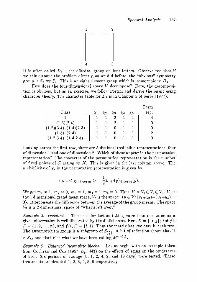
1
4
2
3
Spectral Analysis 157
It is often called D 4 - the dihedral group on four letters. Observe too that ifwe think about the problem directly, as we did before, the "obvious" symmetrygroup is S2 wr S2. This is an eight element group which is isomorphic to D 4.
How does the four-dimensional space V decompose? Here, the decomposition is obvious, but as an exercise, we follow Fortini and derive the result usingcharacter theory. The character table for D 4 is in Chapter 5 of Serre (1977):
PermClass Xl X2 X3 X4 Xs rep.
1 1 1 2 1 1 4(1 3)(2 4) 1 1 -2 1 1 0
(1 2)(3 4), (1 4)(2 3) 1 -1 0 -1 1 0(1 3), (2 4) 1 -1 0 1 -1 2
(1 2 3 4), (1 4 2 3) 1 1 0 -1 -1 0
Looking across the first row, there are 5 distinct irreducible representations, fourof dimension 1 and one of dimension 2. Which of these appear in the permutationrepresentation? The character of the permutation representation is the numberof fixed points of G acting on X. This is given in the last column above. Themultiplicity of Xi in the permutation representation is given by
We get ml = 1, m2 = 0, m3 = 1, m4 = 1,ms = o. Thus, V = VI EBV2 EBV3 • VI isthe 1 dimensional grand mean space, V2 is the space: {y E V: (Yl +Y3)-(Y2+Y4) =O}. It represents the difference between the average of the group means. The spaceV3 is a 2 dimensional space of "what's left over."
Example 3. revisited. The need for factors taking more than one value on agiven observation is well illustrated by the diallel cross. Here X = {{i, j}; i ~ j}.F = {1,2, .. . ,n}, and !{i,j} = {i,j}. Thus the matrix has two ones in each row.The automorphism group is a subgroup of Se;). A bit of reflection shows that it
is Sn, and that V is what we have been calling Mn-2,2.
Example s. Balanced incomplete blocks. Let us begin with an example takenfrom Cochran and Cox (1957, pg. 443) on the effects of aging on the tendernessof beef. Six periods of storage (0, 1, 2, 4, 9, and 18 days) were tested. Thesetreatments are denoted 1, 2, 3, 4, 5, 6 respectively.
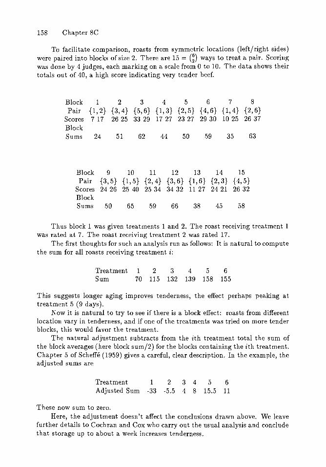
158 Chapter 8C
To facilitate comparison, roasts from symmetric locations (left/right sides)were paired into blocks of size 2. There are 15 = (~) ways to treat a pair. Scoringwas done by 4 judges, each marking on a scale from 0 to 10. The data shows theirtotals out of 40, a high score indicating very tender beef.
1 2 345 6 7 8{1,2} {3,4} {5,6} {1,3} {2,5} {4,6} {1,4} {2,6}7 17 26 25 33 29 17 27 23 27 29 30 10 25 26 37
BlockPair
ScoresBlockSums 24 51 62 44 50 59 35 63
Block 9 10 11 12 13 14 15Pair {3,5} {1,5} {2,4} {3,6} {1,6} {2,3} {4,5}
Scores 24 26 25 40 25 34 34 32 11 27 24 21 26 32BlockSums 50 65 59 66 38 45 58
Thus block 1 was given treatments 1 and 2. The roast receiving treatment 1was rated at 7. The roast receiving treatment 2 was rated 17.
The first thoughts for such an analysis run as follows: It is natural to computethe sum for all roasts receiving treatment i:
Treatment 1 2Sum 70 115
345132 139 158
6155
This suggests longer aging improves tenderness, the effect perhaps peaking attreatment 5 (9 days).
Now it is natural to try to see if there is a block effect: roasts from differentlocation vary in tenderness, and if one of the treatments was tried on more tenderblocks, this would favor the treatment.
The natural adjustment subtracts from the ith treatment total the sum ofthe block averages (here block sum/2) for the blocks containing the ith treatment.Chapter 5 of Scheffe (1959) gives a careful, clear description. In the example, theadjusted sums are
Treatment 1 2 3 4Adjusted Sum -33 -5.5 4 8
5 615.5 11
These now sum to zero.Here, the adjustment doesn't affect the conclusions drawn above. We leave
further details to Cochran and Cox who carry out the usual analysis and concludethat storage up to about a week increases tenderness.
Spectral Analysis 159
In general, there are t treatments to be compared in blocks of size k < t. Anunreduced balanced incomplete block design involves all possible (~) blocks and sok(t) basic units (in the example, t = 6, k = 2 and 30 roasts were involved).
One natural way to index such data is as a pair (i,s) with 1 :s; i :s; t denotingthe treatment applied to that unit, and s of cardinality Isl = k - 1 denoting thesubset in the same block as the given unit. Thus X = {(i, s)} and IXI = t(~=~) =k(%).
The group St that permutes treatment labels operates transitively on X, andwe see that L(X) can be identified with M t -k,k-1,1 of Chapter 7. Another wayto arrive at this result begins with the idea that this experiment has two factors:"treatments" 11 (i, s) = i, and "blocks" 12 {i, s} = {i Us}.
What automorphisms are possible? A little reflection shows that only permutations that permute treatments among themselves are allowed; treatments thatpermute things within a block are ruled out and allowable treatments that moveblocks around can be achieved by permuting treatments. Thus the automorphismgroup is isomorphic to St.
The decomposition now follows from Young's rule. Before stating the result,let us examine the introductory example on aging of meat. Here t = 6, k = 2, andwe have
M 4,1,1 = S6 Ea 2S5,1 Ea S4,2 Ea S4,1,1
dim 30 1 2 X 5 9 10
(see Case 2 of Section B-2 above). The projection onto the one dimensional spaceS6 is the grand mean. The treatment effects can be identified as one of theS5,1 spaces. The block effects space, orthogonal to S6 Ea S5,1, is S4,2 (the fullI5-dimensional block effect space M 4,2 = S6 Ea S5,1 Ea S4,2). These projectionsconstitute the class.ical analysis for this experiment, projecting into treatment andblocks adjusted for treatment.
The remaining SS,l gives a new piece of analysis due to Fortini. To give ita clear interpretation let us change the imagery. Suppose there are 6 amountsof vanilla added to ice cream (from none to a fair amount). Fifteen people eachtaste two servings each in a balanced incomplete block involving 30 servings inall. The treatment effects are interpreted as before. The block effects becomesubject effects - some people are systematically higher than others.
The classical analysis assumes that treatment and block effects are additive.However, this would fail if tasters give ratings partially by comparison. The 2ndcopy of SS,l can be interpreted as the additive effect on the rating of treatment idue to being in the same block with treatment j.
In tasting examples, this (and its higher order analogs described below) makesperfect sense. In the aging/tenderness experiment it seems perfectly sensible toset this effect to zero as is done classically.
To decompose Mt-k,k-l,l in general, Young's rule begins with t - k ones,k -1 twos, and one 3. These are placed into any arrangement as a tableaux whichis non-decreasing in rows and strictly increasing in columns. Thus
k-l k-lMt-k,k-I,I = st EB 2St- j,j Ea St-k,k EB st- j-I,M.
j=l j=l
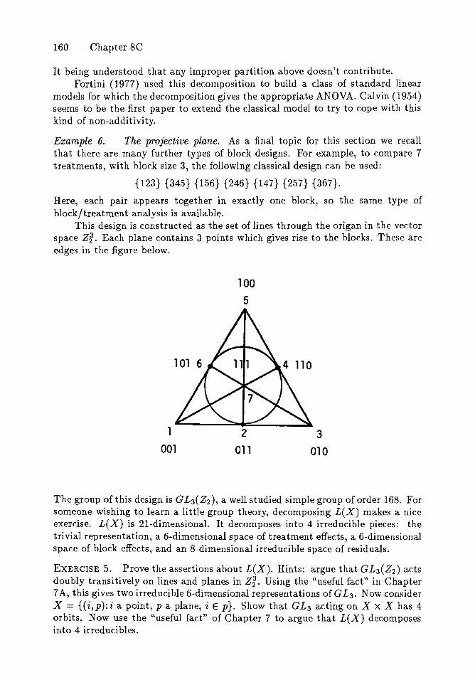
160 Chapter 8C
It being understood that any improper partition above doesn't contribute.Fortini (1977) used this decomposition to build a class of standard linear
models for which the decomposition gives the appropriate ANOVA. Calvin (1954)seems to be the first paper to extend the classical model to try to cope with thiskind of non-additivity.
Example 6. The projective plane. As a final topic for this section we recallthat there are many further types of block designs. For example, to compare 7treatments, with block size 3, the following classical design can be used:
{123} {345} {156} {246} {147} {257} {367}.
Here, each pair appears together in exactly one block, so the same type ofblock/treatment analysis is available.
This design is constructed as the set of lines through the origan in the vectorspace Z? Each plane contains 3 points which gives rise to the blocks. These areedges in the figure below.
100
5
1
0012
0113
010
The group of this design is GL3 ( Z2), a well studied simple group of order 168. Forsomeone wishing to learn a little group theory, decomposing L(X) makes a niceexercise. L(X) is 21-dimensional. It decomposes into 4 irreducible pieces: thetrivial representation, a 6-dimensional space of treatment effects, a 6-dimensionalspace of block effects, and an 8 dimensional irreducible space of residuals.
EXERCISE 5. Prove the assertions about L(X). Hints: argue that GL3(Z2) actsdoubly transitively on lines and planes in Z? Using the "useful fact" in Chapter7A, this gives two irreducible 6-dimensional representations of GL3 • Now considerX = {(i, p): i a point, p a plane, i E p}. Show that GL3 acting on X X X has 4orbits. Now use the "useful fact" of Chapter 7 to argue that L(X) decomposesinto 4 irreducibles.
Spectral Analysis 161
This example is the tip of the iceberg called combinatorial design. Lander(1982) is a nice reference for the construction of block designs. Beth, Jungnichel,and Lenz (1986) is a recent encyclopedic reference. It seems like a worthwhileproject to go through the classical designs, compute automorphisim groups, andcompare the spectral decomposition with classical ANOVA.
D. THOUGHTS ABOUT SPECTRAL ANALYSIS.
This chapter builds on two well established traditions: the analysis of varianceand the spectral analysis of time series. The new applications and variations ofclassical areas such as block designs should be regarded speculatively.
There is much of value in the parent theories as they appear in modernpractice which I have not thought through in sufficient detail to carry over. Thissection outlines some of these techniques.
1. Why projections onto invariant subspaces? It is an empirical fact that thedecomposition of data indexed by X into irreducible pieces is sometimes scientifically useful. Let me make an attempt to explain this. There is no one right wayto analyze data. The spectral decomposition presents certain averages of the datawhich often seem sensible. The set of all averages is a 1-1 function of the data, sonothing is lost. Often the specific labeling of X is fairly arbitrary, and we wouldrather not have our conclusions depend on this labeling. In other circumstances,the order is worth taking into account, but it is useful to separate the part of theanalysis that depends on the order from the part that is invariant under G.
Data indexed by X are represented by a function on X. Sometimes thisfunction takes values in the integers, as in the case of counted data: "how manypeople in the population chose X?" Even here we want to be able to talk aboutaverages and differences of averages, so we need to consider functions from X intothe rationals Q. For the permutation group, the splitting of a representation overQ is the same as its splitting over the real or complex numbers.
Our function thus naturally sits in L(X): the set of all complex valuedfunctions. A subset of L(X) can be thought of as a partial description. In practicethese will be things like the constants or "first order functions;" sets of functionsthat are simple to describe or interpret. If the actual f can be well approximatedby a simple I we regard this as useful. If I is "first order" and 9 is "first order"it seems natural that ~ f or f +9 be the "first order" since, for example, f +9has the interpretation of combining the two data sets (for counted data). Thissuggests that a basic partial description be a subspace of L(X).
Finally, if G acts on X we want to consider descriptions that don't dependon the labelling: it seems unnatural that I(x) could be "first order" but notf(gx). Thus a natural descriptive unit is an invariant subspace of L(X). Thenspectral analysis is the decomposition of f( x) into its projections on the irreducibleinvariant subspaces of L(X), and the approximation of f( x) by as small a numberof its projections as give a reasonable fit.
Of course, this kind of linear analysis is just a start. Non-linear analyses mayalso be most useful (see Section (4) below). These are easiest to interpret if theyhave a simple connection to the linear theory (log f may be well approximated
162 Chapter 8D
by a simple linear fit).2. On the choice of group. Spectral analysis begins with a group G acting on
a set X. In some areas, like ANOVA, there is some theory to guide the choice of G.In other areas, like time series, physics dictates the choice. In new applications,there may be several possible groups among which to choose.
Clearly if G acts on X and H is a subgroup of G, the splitting of L(X) into Hirreducibles is finer than the splitting under G. Choosing the smallest group thatpreserves essential structure gives the largest number of projections. Preliminaryanalysis may start with larger groups.
Consider a two way I X J array. The group that gives classical ANOVAis SI X SJ. Another group that operates transitively is ZI X ZJ, operating bycyclically shifting each coordinate. A third transitive action is given by SI X ZJ.Any of these groups might be appropriate. ZJ preserves adjacency (or time order)while SI invariance says adjacency isn't relevant. Thus SI X ZJ might be deemednatural for a problem in which the rows index types of bird, the columns indexmonths of the year, and the entries are number of birds sighted in that month bya local bird watching society.
EXERCISE 6. Derive the appropriate spectral analysis for SI X ZJ.As a second example, consider X == Z~. Four groups act naturally on this
space: Z~, G L k (Z2), Z2 wr Sk, and Z2 wr Zk. We consider these in turn.a) Under Z~, L(X) == Et) Vy where Vy is the one dimensional space spanned
yEX
by x ~ ( -1 )Xoy• Here spectral analysis amounts to the Fourier inversion theorem
f(x) = 21k L( -lY'Y j(y).y
b) GL k (Z2) acts doubly transitively on X, so by Serre's exercise (2.6),
L(X) == Vo ffi VI
with Vo the constants and VI == {f: ~f(x) == O}.c) Z2 wr Sk (see Section C for notation) is the group of pairs (y,1r) with
1r E Sk, Y E Z~ acting on X by (y,1r)x == (X 1r-l(I) + YI, ... ,X1r-l(k) + Yk): youpermute the coordinates by 1r and add y. It is straightforward to show that
with Vj the linear span of (_l)X oy for Iyl == j. Thus spectral analysis under Z2 wrSk lumps together pieces of the spectral analysis under G == Z~.
EXERCISE 7. Show that L(X) splits as shown for Z2 wr Sk. Find the decomposition with respect to Z2 wr Zk.
3. On probability. The data analytic approach to spectral analysis presentedin this chapter is not based on probability. Spectral analysis is a reasonable, usefulactivity if f is not a sample, rather a complete enumeration of a population. Thus,
Spectral Analysis 163
nothing is unknown, but there may still be plenty to do in condensing the data sothat simple descriptions can be given. This point of view follows Tukey (1977).
Of course, there are many opportunities for probability to play a role. Whenwe informally assess goodness of fit in a linear approximation such as f( i, j) ==a + bi + Cj, we compare the residuals rij = f(i,j) - a - bi - Cj, with the maineffects a, bi , Cj. If residuals are small, we regard the approximation as useful. Thestandard tests and confidence interval procedures are formalizations of this idea.
There is much more to do in constructing a believable probabilistic theoryfor spectral analysis. For example, the data f(x) might be a sample from alarger population F(x). If the sample size is small, there is no reasonable hopeof estimating F, but one can hope to estimate some simple functionals of F suchas its projections onto a few subspaces of interest. How the dimensionality of thesubspaces should relate to the size of X and the sample size seems like a richinteresting question. Finch (1969) makes a start on these questions. See also thediscussion in Section 3 of Diaconis (1985).
In some instances the bootstrap offers a reasonable way to wiggle data abit. There are two obvious ways to bootstrap - sample iid from f( x) to getflex), f 2(x), ... , fb(x), or fit a model and bootstrap residuals. Freedman (1981)describes these alternatives in regression problems. Of course, all of this is tied tosome sampling like story. Without a believable sampling justification (as in complete enumeration problems) I find the bootstrap far too violent a perturbationof the data. Diaconis (1983) suggests less drastic perturbations.
I have been impressed with the usefulness of the basic normal perturbationmodel outlined in Section A-3. This serves as an accurate approximation for allsorts of schemes for quantifying "if the data had come out different, how wouldmy conclusions differ?" or "if I had more data, how close is my best guess likelyto be?"
Some further discussion of the need for probability is given later. It is worthemphasizing that spectral analysis can be useful without underlying probabilisticstructure.
4. Lessons from ANOVA. A basic component of ANOVA is a test to see ifprojection of a given function onto a given subspace can be assumed to be zero.The standard test involves comparison of the observed projection with an estimateof "ambient noise" - usually the normalized length of the projection of the dataonto the space of residuals. If the ratio of lengths is "large", then the projectioncannot be asserted to be zero. Usually, "large" is quantified under the normalperturbation model of Section A-3.
Terry Speed (1987) gives an elegant survey of this material delineating anatural class of perturbation models involving patterned covariance matrices, for\vhich the orthogonal projections in fact give the maximum likelihood estimates.
An important idea from classical ANOVA deals with fixed versus random effects. As data analytic motivation, consider a two way array with one observationper cell. Suppose the rows are different brands of typewriters and the columnsare different typists. The Xij might be average speed. If we are trying to evaluate typewriters, then the row averages are basic. It may be that the typists arethought of as drawn from a pool of typists. Then, the column averages are not of
164 Chapter 8D
particular interest - they are thought of as random effects. Their mean, variance,or distribution may be of interest as information about the population of typists.Tukey (1961) contains an interesting discussion of the distinction between fixedand random effects and its impact on ANOVA and time series data.
Modern ANOVA employs a wealth of non-linear techniques. These beginwith transformations of Xij to T(Xij) aiming for linearity. Box and Cox (1964)or Hoaglin, Mosteller, and Tukey (1983, Chapter 8) give the basics. This is oftensupplemented by fitting more complex models such as
as in Tukey (1949) or Mandel (1961). Stein (1966) gives a decision theoreticversion.
More aggressive transformation techniques involving splines or more complexsmoothers appear in approaches like projection pursuit (see, e.g. Huber (1985) orHenry (1983)) or Ace (see Breiman and Friedman (1985), Stone (1985), or Hastieand Tibshirani (1986)). None of these techniques are well tried out in ANOVAsettings, but all seem worth thinking about and extending to other instances ofspectral analysis.
Another important aspect of modern statistics is a concern for robustness it may be that observed data is well approximated by a linear fit except for a few"wild values." For methods based on linear projections, even one wild value canfoul up everything, making it seem as if no linear fit works.
One approach to these problems is to replace the usual averaging operators byrobust versions such as medians. Hoaglin, Mosteller and Tukey (1985, Chapters2-5) contains a good review. It is not at all clear if these approaches can beadapted to more complex designs which really lean on the additivity. Anotherapproach is to try to remove or down-weight the outliers. Other approachesinvolve using perturbation distributions that are longer tailed than normal. Pasta(1987) contains a review of the problems and available remedies. It is fair to saythat even for ANOVA this is a difficult problem, on the cutting edge of currentresearch.
Here is another contribution of modern statistical theory to ANOVA. Wenow realize that while the projections have many appealing properties, they arenot the most accurate estimates of population projections under the usual normalmodel. Non-linear shrinkage estimators can do better than the classical linearestimators. Stein (1966) shows how to modify the usual estimators in orthogonaldesigns to get improvement. I do not know of a systematic account for moregeneral designs.
The Bayesian analysis of ANOVA data is important on its own - we oftenknow quite a bit and want a way to combine this prior knowledge with the observations in a sensible way. Box and Tiao (1973) cover the basics. Consonni andDawid (1985) give group related theory.
The Bayesian techniques give a reasonable way to get shrinkage estimates,possibly using conjugate priors and empirical Bayes ideas as surveyed by Morris(1983). Berger (1985, Chapter 4) surveys the recent literature on estimating a
Spectral Analysis 165
normal mean. Again, most of these ideas are applicable in ANOVA and otherspectral analysis problems but the details need to be worked out on a case bycase basis.
An important problem that must be dealt with is missing data. The algebraictheory of ANOVA works neatly if things are neatly balanced. With a two-waylayout and unequal numbers of observations per cell, there are no longer simpleform~las for many quantities of interest. It is not unusual to have symmetrybroken by having some subjects get sick or be lost for other reasons.
A rich collection of techniques has evolved for dealing with these problems.A most useful tool for computing "projections" has evolved as the EM algorithmof Dempster, Laird and Rubin (1977). They survey the literature. Dodge (1985)gives some special techniques for ANOVA problems.
There is some very recent work which relates the approach taken in thischapter to some of the mathematics of Chapter 3-F. In working with stochasticmodels for designed experiments, many workers have emphasized the importanceand utility of "general balance." This is a condition introduced by Nelder (1965)which links the "design" part of the experiment to the structure of the assumedmodel. When the condition holds, all sorts of elegant formulas for computing bestlinear unbiased estimates are available. A recent survey of this material is givenby Houtman and Speed (1983).
Recently, Bailey and Rowley (1986) have given a useful sufficient conditionon the group of symmetries of the design (the definitions are a bit different thanthose in Section C) which forces generalized balance. There are too many detailsneeded to state their results carefully. Very roughly, the group of symmetries actson a space T of treatments, and the representation L(T) must be multiplicityfree (see Chapter 3F). The Bailey and Rowley paper is very clearly written andconnects wonderfully with the material in this monograph.
5. Lessons from time series. Spectral analysis of time series and other signals is widely applied and has an enormous literature. Robinson (1982) surveys itshistory. It differs from ANOVA in having numerous hard science manifestations.Indeed, in some speech, geophysics, and signal processing applications the spectrum is naturally observed. Brillinger (1988) contains a list of such applications.
It is natural to try to emulate the success stories of spectral analysis for othergroups. It seems fair to admit that at present there is no underlying "physicaljustification" for the spectral decomposition in other cases. None the less, it seemspromising to try to plug into the experience and imagery of the established theory.
For example, it is well known that the periodogram (essentially the squareddiscrete Fourier transform) is not an accurate estimate of the amplitude of theFourier transform at given frequency. It is asymptotically an exponential variable,and so not consistent as time goes on. Under smoothness assumptions on theunderlying spectrum, smoothing the periodogram becomes sensible and leads toreasonable estimators. Olshen (1967) gives details.
The same problem is present in other spectral analyses. Under the normalperturbation model the Fourier transform has independent coordinates with fixedvariance (see Example A-3). This continues to hold under broad alternative perturbation models. Without repeated observations, there is a limit to the accuracy
166 Chapter 8D
of estimates. Thought of in the ANOVA context this is not surprising - we canonly hope for an accurate indicator of variability. We can think of formulatingnatural smoothness assumptions to allow increased accuracy.
When applicable, the sampling model is a natural replacement for signal plusnoise - the Fourier transform applied to a population is simply a 1-1 transformand so gives a natural parameter to estimate.
Time series has goals in addition to estimating the spectrum at a point.In continuous time problems, there can be a continuous spectrum, and manyother functionals are relevant. Tukey (1986) emphasizes this aspect and pointsto properties of ensembles of time series that are of scientific interest. For rankeddata, there is an obvious prediction problem: how will a complete enumeration(or larger sample), turn out? More in line with time series, prediction mightbe this: people partially rank several quantities; later their true preferences arerevealed. How good a guess can be made based on current knowledge?
Time series analysis has a time domain side which is based on models forthe observed process. There is a healthy interplay between time and frequencydomains. This is presented by Anderson (1971) or Priestly (1981). As withANOVA, it's nice to see natural projections have an interpretation as reasonableestimates of parameters in a model. Models for data on homogeneous spacesare introduced in the next chapter. There hasn't been any serious work on theinterplay with spectral analysis.
There are many modern versions of spectral analysis of time series. Thereare remedies for all of the problems discussed in the ANOVA section. It seemsimpossible to survey this briefly. Anderson (1971), Brillinger (1975) and Priestly(1981) are good references; leading to others. With work, most of these ideasshould be transferrable to other spectral domains when the need arises.
One final thought: real examples in hard science settings are a sparklingpart of time series analysis. If progress is to be made in generalization, similarexamples will have to be found.
Chapter 9. Models
Fitting models to data is a popular activity. For data taking values in a groupor homogeneous space, the associated representation theory gives neat families ofmodels. Briefly, if P(x) is a probability on X, write P(x) == eh(x) with h == log P.Then expand h in a natural basis bi of L(X):h(x) == ~(Jibi(X). Any positiveprobability can be expanded in this way. Truncating the expansion to a fixednumber of terms leads to families of simple measures or models; because bi areorthogonal, (}i are identifiable.
It is an interesting fact that many models introduced by applied workersfall into this class. The general story is presented first, then a specialization todata on spheres, then a specialization to partially ranked data. A brief review ofother approaches to ranked data is followed by a section supplying the relevantexponential family theory.
A. EXPONENTIAL FAMILIES FROM REPRESENTATIONS
Let G be a group acting transitively on a compact set X. Let L(X) denote thereal valued continuous functions on X. Suppose X has an invariant distributiondx. The following abstracts an idea introduced by Lo (1977) and Beran (1979).
Definition. Let 0 be an invariant subspace of L(X) containing the constants.Define a family of measures, one for each () E 0, by specifying the densities to be
Po(dx) = a((J)eO(x)dx,
where a((}) is a normalizing constant forcing Po (dx) to integrate to 1.Suppose 0 is finite dimensional. Let bo =constant, bI , b2 , ••• , bp be a basis
for 0. Then the family can be parameterized as
LEMMA 1. The family * is well parameterized in the sense that Po = Po' if andonly if 0 =0' .
Proof. Only the forward direction requires proof. If Po = PO', then
(8 - 8') · b(x) = log(a(8') / a((})) for all x.
The left side is a linear combination of bI , b2 , ••• , bp which is constant. But1, bI , b2 , ••• , bp is a basis, so () = 8'. 0
In applications there is a decomposition into invariant subspaces L(X)Vo E9 VI E9 V2 E9 ... and 0's are chosen as a finite direct sum of subspaces. Usually
167
168 Chapter 9A
these nest together neatly to form zeroeth order models (the uniform distribution),1st order models, etc. The matrix entries of the irreducible representations thenprovide a convenient basis.
The easiest example is for data on Z~. The exponential families that thegroup theory suggests are exactly the log-linear models that statisticians fit to2 X 2 ... X 2 tables (k factors). Here a person is classified via k dichotomousvariables. This gives rise to a vector in Zf or locates a cell in the table.
A useful entry to the statistical literature is provided by the first few chapters of Gokhole and Kullback (1978). General contingency tables can be treatedsimilarly. Since this is such a well studied area, we will not pursue it further thanmentioning the important paper of Darroch, Lauritzen and Speed (1980). Thisgives an elegant interpretation to setting (Ji = 0 for a large class of models. Itwould be an important contribution to generalize their ideas to the general groupcase.
The measure Fo(dx) governs a single observation. We model a sample of sizen by a product measure
n
P8(XI, X2,···, x n ) = IT P8(Xi) dx i.i=l
The statistical problem becomes, given a model El, and observations Xl,
X2, ••• ,Xn , what is a reasonable guess for 8, and how sure are you about theanswer.
Remark 1. Crain (1973, 1974, 1976) suggested expansion of log P(x) in abasis of orthogonal functions as a route to nonparametric density estimation. Hetruncated the expansion at a point depending on sample size. This leads to anapproximate density in a finite dimensional exponential family as in the definitionabove.
Crain's later papers give conditions on how large the cutoff point should beto have the maximum likelihood estimator exist. These are discussed in SectionE below.
Remark 2. There is a growing literature on orthogonal series estimators density estimators based on expanding the density directly as P(x) :::: ~(}ibi( x).Hall (1986) makes noteworthy contributions providing simple useable estimatorsand giving sharp rates of convergence. He gives pointers to the literature. Hall'sresults can be carried over to problems on compact homogeneous spaces in astraightforward way.
Orthogonal series estimators suffer from the possibility of negative densityestimates. This is why Crain worked with log P(x). It is a worthwhile project tocombine the ideas and bounds of Hall with the ideas of Crain.
Remark 3. One problem encountered with log P: it is badly behaved if P :::: o.Consider a density on the circle. If P(x) > 0 outside an interval, things can berescaled and there is no trouble. If P(x) :::: 0 on several intervals the problemcan be treated as a mixture, but the log P approach is wearing out its welcome.

Models 169
There are so many other density estimates possible - from histogram's, throughkernel estimators, through projection pursuit.
On more gene'ral homogeneous spaces, problems with vanishing density seemeven less approachable.
Remark 4. The definition above is in terms of real valued functions. This worksfine for the symmetric group and its homogeneous spaces and for the orthogonalgroup. In general, L(X) may be taken as all cO'mplex functions and a model maybe taken as an invariant subspace of L(X). Just as any real function on Zn canbe expanded in terms of sin(21rjk/n) and cos(21rjk/n), any real function on Xcan be expanded as a real linear combination of the real and imaginary parts ofthe matrix entries of the irreducible representations that occur in the splitting ofL(X).
Remark 5. The models intro.duced here blend in nicely with the spectral theoryof Chapter 8. They are the largest models which allow as sufficient statistics theingredients of the matching spectral analysis. See E-1 below.
Remark 6. The ideas set out above can be generalized in various ways. Onenatural extension begins with a space X and a symmetric Markov chain P( x, dx)on X. Symmetric chains can he orthogonally diagonalized, and the eigen vectorsprovide a convenient orthogona,l basis for L(X). There are chains that don'tarise fro·m groups where this b·asis can h.e written explicitly. See Banni and Ito(1986, 1987) or Diaconis and Smith (1987). It is not clear if these models can beconnected to the underlying chain.
A word of caution: I find the statistical community introduces models much tooeasily. In some cases, there is a justification: "height is the sum of a lot of smallfactors, so heights should be approximately normally distributed" or "the numberof accidents is the sum of a lot of roughly independent binomial variables withsmall parameters, so accidents should be approximately Poisson." In some caseslinearity or physical justification (and repeated comparison with reality) justifymodels: Gauss' discovery of Ceres, Bright-Wigner distributions in particle physicsor multinomial distributio,ns in genetics are examples.
Th'e cases where some slim justification is given seem alarmingly few to me.Usually, one is contemplating some data and it model is chosen for convenienceas a way of doing data analysis. This is a curve fitting approach and is fine,except that the p.roduct model assum-es independence. Further, the assumptionsab·out P8(dx) may be a drastic oversimplification. One may well do b'etter lookingdirectly at the data using spectral analysis, or a convenient ad hoc ap-proach.
I must admit that I too find ad hoc modeling attractive and occasionallyuseful - it seems like a most worthwhile project to try to isolate what good comesout of the modeling paradigm an·d attempt to build a theory that optimizes thisgood instead of behavior in El, non-existent fantasy lan·d of iid repetitions.
170 Chapter 9B
B. DATA ON SPHERES.
Spherical data is discussed in Chapter 5-C. One important special problemis testing for uniformity. A large number of special tests have been suggested.These are reviewed by Mardia (1972) and Watson (1983). We discuss here one ofthe earliest tests and follow its later developments.
Let Xl, X 2 , ••• , X n be unit vectors on the sphere BP in p dimensions. Definethe sample resultant R and sample mean direction U(8) by
1~ --- L.J Xi = RU(8).n i=l
Intuitively, if Xi are uniform, R will be "small" because there will be a lot ofcancellation. If Xi are non-uniform and cluster around some point, then R willbe "large." Rayleigh (1919) worked out the distribution of R under the uniformdistribution and could thus propose a test "reject uniformity if R > r" where ris chosen to achieve a given proportion of false rejections. A nice derivation ofRayleigh's results is given by Feller (1971, pg. 32).
Questions and alternate tests immediately suggest themselves. Observe thatRayleigh's test is invariant: R does not change if Xl, X 2 , ••• , X n , are replacedby rXl, ... , r X n , r orthogonal. On the negative side, Rayleigh's test would notbe appropriate if the Xi tend to cluster either close to a point or its antipode.When is this test a good one? Some answers have come from statistical theory.
Independent of Rayleigh, a class of natural non-uniform distributions wasdeveloped and used by Von Mises and Fisher. These have the form
with x E BP, dx the uniform distribution, JL E BP, and k 2:: o. The normalizingconstant is
Cp( k) = k(p-l)/2 / (21r )p/2 I(p-I)/2 (k)
with I r ( k) the modified Bessel function of the first kind.The PJ.t,k have "mean direction" JL and as k increases are more and more con
centrated about JL. They arise naturally from the first hitting place of a Brownianparticle with drift on the sphere. Watson (1983, Chapter 3) discusses this andother justifications.
A nice result is that the likelihood ratio test of
Ho: k = 0 vs. HI: k > 0, JL unknown
reduces to Rayleigh's test. Further, Rayleigh's test is the uniformly most powerfulinvariant test of uniformity versus PJ.t,k(dx). These results are due to Beran (1968)who discusses their analog on compact homogeneous spaces. Gine (1975), Wellner(1979), and Jupp and Spurr (1985) amplify and develop these ideas. Closelyrelated developments in the signal processing literature are surveyed by Lo andEshleman (1979).
Models 171
These developments give a pleasing answer to the original question: when isRayleigh's test good - it's good if data cluster about one point JL in a sphericallysymmetric way.
Remark. I cannot resist reporting some background on Fisher's motivation forworking with the distribution discussed above. This story was told to me in 1984by the geologist Colin B. B. Bull. Dr. Bull was a student in Cambridge in theearly 1950's. One day he ran across the street in haste and knocked an old manoff a bicycle! The old man seemed dazed. When asked where he was boundhe replied "India." It turned out to be R. A. Fisher who was meeting a trainenroute to a visit to the Indian Statistical Institute. A month later, Bull metFisher at Cambridge and again apologized. Fisher asked what area Bull workedin. Bull explained that a group of geologists was trying to test Wegener's theoryof continental drift. Wegener had postulated that our current continents used tonest together. He tested this by looking at the distribution of a wide variety ofbird, animal and plant life - arguing that matching points had close distributions.
Geologists found themselves far afield in trying to really understand Wegener's arguments. They searched for data that were closer to geology. They hadhit on the distribution of magnetization angle in rocks. This gave points naturallydistributed on the sphere. They had two distributions (from matching points ontwo continents) and wanted to test if the distributions were the same.
Fisher took a surprisingly keen interest in the problem and set out to learnthe relevant geology. In addition to writing his famous paper (which showed thedistributions were different) he gave a series of talks at the geology department tomake sure he'd got it right. Bull told me these were very clear, and remarkablefor the depth Fisher showed after a few months study.
Why did Fisher take such a keen interest? A large part of the answer maylie in Fisher's ongoing war with Harold Jeffries. They had been rudely battlingfor at least 30 years over the foundations of statistics. Jeffries has never reallyaccepted (as of 1987!) continental drift. It is scarcely mentioned in Jeffries' bookon geophysics. Fisher presumably had some extra-curricular motivation.
The motivation for Rayleigh's and Von Mises' work seems equally fascinating!Watson (1983, Chapter 3) gives a good set of pointers.
There is a second family of probabilities on BP that has received a good dealof attention. The Bingham densities are defined on BP as
bp(D) exp{tr[DR'xx'R]}dx
where D is a p X P diagonal matrix with (p, p) entry zero, and R is a p X Porthogonal matrix.
These densities are invariant under x ---+ -x and so are possible models forunsigned directional data - lines in RP (or points in projective space). A host ofproperties and characterizations of these densities are known.
Beran (1979) points out that both the Fisher-Von Mises and Bingham familiesfit nicely with the definition of models given in Section A. Here, the group SO(p)of p X P orthogonal matrices with determinant 1 operates transitively on the spaceX = BP. Take L(X) as the continuous real valued functions on X.
172 Chapter 9C
Let Pk be the homogeneo·us polynomials (in RP) of degree k. Let M k be theP2
subspace of harmonic functions in Pk : Mk = {f: \/2 f :::: O} where \12 = E /;rei:o::l I
Thes·e Mk are invariant and irreducible under the action of SOp. Further, L(X) =ffik£oMk as a Hilbert space direct sum. Proofs are in Dunkl and Ramirez (1971).
Following the definition, Mo - the zero-th order model gives only the uniform distribution. Mo ffi M1 - the first order models is o;bviously spanned by1, X1,X2, ••• ,xp (these are all killed by \]2). The associated exponential familyis the Fisher-Von Mises family.
A second-order model is defined by Mo ffi M 1 ffi M 2 • B·eran (1979) sh·ows theseare spanned by{XiX j}- {x;}, giving the Bingham distribution. In general, a basis
rfor ffi M k consists of all distinct monomials of degree r a.nd r -- 1, excluding x;
k=()if r is even or x;-1 if r is odd.
Some more technical discussion of estimates and their properties is given inSectio.n E below.
C. MODELS FOR PERMUTATIONS AND PAltT1ALLY RANKED DATA.
Begin with a data set on the symmetric group S"". Say I( 1r) is the proportionof the data choosing rankn,g 1r. In working; with stlch data it seems natural tobegin by looking at first order statistics: the proportions ranking each item first,or last, and more gen~rally the proportion ranking item i in position j. Theaverage rank given ecteh item is a popular summary which is a mean of these firstorder statistics.
Paul Holland suggested working with the ex.ponential family throu..gh the firstorder statistics in the ea.rly 1970's. This leads to
Holland's model. Let p be th'e n - 1 dimensional irreducible representation of Sn.Let Mat(n - 1) be the set of all n - 1 by n, ..-- 1 real m-atrices. Define
P,(1f) := c(O)eTr [9 p(1r)]; for (J'E Mat(n - 1),
with c(8)-1 = ~1r eTr( 8(p( 11"» .
Remarks. These models are well parameterized by IJ E Mat(n -1) = R(n-l)2.
To give a.n example, consider a simple sub family:
This can be described intuitively as "there is some special chance of ranking item1 in position 1; whether or not this is done, the rest of the permutation is chosenuniformly.
If item 1 were carefully ranked, and then the others chosen at random, theappropriate family would be
Holland's model exten.ds these considerations to a full first order model.
Models 173
Joe Verducci (1982) began with Holland's model and the observation that(n -1)2 parameters is still a lot to work with and think about. He introduced somenatural low dimensional subfamilies and fit them successfully to real data sets.One of his nice observations is that some of Mallows' metric models introducedin Chapter 6-A-1 are subfamilies of first order exponential families.
Consider
Q)..(1r) = c(A)eAH(1r,rro) A E IR, H = Hamming distance.
For fixed 1ro, this is a subfamily of Holland's, taking () = Ap(1r01). Of course, if
1ro is also treated as a parameter, the two models are different. Verducci observedthat replacing H by Spearman's S2 also gives a first order model.
Arthur Silverberg (1980) began to work with second order models using theproportion ranking i, i' in position j, j'.Verducci (1982) realized the connectionwith group representations could help sort out questions of when a model is full,or well parameterized.
Silverberg worked with q-permutations, where people rank their favorite q outof n. This would be data on Sn/Sn-q in the language of Chapter 7. Generalizingslightly, let A be a partition of n. Let X = Sn/ SAl X SA2 ••. X SAk be the set orpartial rankings of shape A. Using Young's rule, and notation of Chapter 7,
L(X) = MA = EB k(vj >')SVlI~n
where the sum is over all partitions v of n which are larger than A in the partialorder of majorization and k(v, A) is the multiplicity of 8 11 in MA. See the remarksto Theorem 1 in Chapter 7A. Restricting attention to a few of the pieces in thisdecomposition gives models of various sorts.
If A = (At, ... , Ak), the n -1 dimensional representation appears (k -1) times(k( n - 1, 1); A) = k - 1). The direct sum of these k - 1 dimensional subspaces hasdimension (k - 1)(n - 1) and it spans the first order model.
Let us apply Young's rule to answer a question posed by Silverberg (1980) what is the dimension of 2nd order models for q-permutation data. The partitioninvolved is n - q, 1q. Suppose that 2 ~ q ~ n - q. Second order models are associated with partitions (n - 2, 1, 1) and (n - 2, 2). By Young's rule, the multiplicityof each in M t
q ,n-q is (~). By the hook length formula of Chapter 7, the dimensionof sn-2,1,t is (n - l)(n - 2)/2. The dimension of sn-2,2 is n(n - 3)/2.
If we also include the first order component, the dimension of the secondorder model is
( -1) (q)(n-1) (q)n(n-3)qn +22 +22·
Of course, it is important to keep the pieces separated, both for computation andinference.
The models discussed above have not been broadly applied. At present, thereare no simple processes that lead to these models, nor simple interpretations orbenefits from them. Since exponential families have such a good track record in
174 Chapter 9D
these directions, it seems like a worthwhile project to study and develop propertiesof low order exponential families on partially ranked data.
Some technical and practical aspects of the models in this section are discussed in Section E of this chapter.
D. OTHER MODELS FOR RANKED DATA.
The models proposed for ranked data in the previous section and the metricmodels of Chapter 6 have a distinctly ad-hoc flavor to them. There have beenenergetic attempts in the psychological literature to develop models for rankeddata that are grounded in some more basic processes. This section briefly describessome of the models and gives pointers to the literature.
.To fix a problem, consider an experiment in which p tones are played for asubject who is to rank them in order of loudness. It is an empirical fact thateven a single subject, asked to repeat this task on different days, gives differentanswers. To account for this variability, Thurstone introduced an unobservable"discriminal process" of the form UI +XI , U2 +X2 , ••• up+Xp where UI, U2, • •• , Up
are fixed constants, and Xl, ... , X p are random variables, independent with thesame distribution. It is postulated that on a given trial, a subject rank orderstone i in position j if Ui + Xi is the jth largest.
Thurstone proposed normal distributions for the Xi. With a distributionfixed, one can estimate best fitting Ui and compare data and model. There hasbeen a lot of experimental work showing a good fit for certain tasks. An extensive,readable review of this work appears in Luce and Suppes (1965).
A second line of work stems from a simple model put forward by Luce (1959).This postulates an unobservable system of weights Wl, W2, ••. ,wp• It is proposedthat a subject ranks items by choosing the first ranked item with probabilityproportional to W i . This choice being I, the second ranked item is chosen withprobability proportional to {Wj} - WI, and so on.
This model has also been fit to data with some success. Holman and Marleyproved that if the underlying random variables Xi in Thurstone's approach havean extreme value distribution P{X < t} = e-e-', -00 < t < 00, the resultingchoice probabilities are given by Luce model as well. Yellott (1977) gives references, proves a converse, and suggests some intriguing open probability problems.
Yellott's results deal with location shifts of extreme value distributions. LouisGordon (1983) has observed a neat reformulation: consider the basic weightsWl, • • · w p in Luce's model. Let YI , 1'2, ... Yp be independent and identically distributed standard exponential variables: P(Y > t) = e- t . Put a probabilityon permutations by considering the order statistics of Y1/WI, ... , Yp/wp. Cordonshows this induces the distribution of Luce's sequential model. Since the log of anexponential variable has an extreme value distribution, this is a special case of theresults described by Yellott. Gordon shows how to use the representation to givean efficient algorithm for generating random permutations from this distribution.
Independent of the literature cited above, Plackett (1975) developed a familyof non-uniform probabilities on permutations. Plackett's first order models arethe same as the Luce models. These are fit to some race horse data by Henery
Models 175
(1981). An order statistics version of Plackett's higher order model is given byDansie (1983). Plackett's motivation is interesting. One has available data onthe chance that a horse finishes first in a race. One wants to predict the chancethat the horse "shows" (finishes in the top 3). Plackett fit a model on the finalpermutation using the first order data. This approach is the basis of severalbelievable systems for beating the races. See Zambia and Hausch (1984).
Models like Luce's have been extended, axiomatized, and tested by modernmathematical psychologists. The extensions account for practical difficulties suchas the irrelevance of alternatives. If Luce's model is taken literally, one postulatesa weight associated to the ith object independent of the other choices available.This easily leads to thought experiments generating data at variance with such amodel. The following example is due to L. J. Savage.
Suppose you are indifferent between a trip to Paris and a trip to Rome.Thus w(Paris) == w(Rome). You clearly prefer Paris + $10 to Paris. On Luce'smodel, if asked to choose between Paris, Paris + $10, or Rome, you choose Romeabout 1/3 of the time. Something is wrong here - it is unlikely that such asmall inducement would change things so drastically. Tversky (1972) gives otherexamples and discussion.
One simple way around this objection is to allow the weights to depend onthe problem under consideration. Going further, after the first choice is made,the second choice can be modeled by a new set of weights. But then any set ofchoice probabilities can be matched exactly so no test of the model is possible.
Some interesting half-way houses have been worked out. For example, Tversky (1972) describes choice by a hierarchical elimination process. Each alternativeis viewed as a collection of measurable aspects. To make a choice, one selects anaspect with probability proportional to its measure. This eliminates all alternatives not possessing this aspect. The process continues until one alternativeremains. For example, in choosing a restaurant for dinner, we may first choosetype of food (e.g. seafood), then location, then price. Tverskyand Sattath (1979)consider a subclass of these hierarchical models called preference trees which havemany appealing properties.
The present state of the theory is this - no one claims to have a reasonable,believable and testable theory of how we perform ranking or choice. There is alist of constraints and desiderata on potential theories. These offer insight intochoice behavior and rule out many naive suggestions. Thurstone's models andLuce's model are seen as straw men which triggered these investigations. Slightelaborations of these models have proven useful in horse race betting.
E. THEORY AND PRACTICAL DETAILS.
1. Justifying exponential families.
Return to the setting of Section A - exponential families on a space X. Onejustification for these models Pe that statisticians have developed goes as follows.Consider first a sample Xl, X 2 , •• • X n from such a family with unknown o. The
176 Chapter 9E
sufficient statistics are
Any question about which () E 0 generated the data can be answered as well fromthe averages bi as from the full set of data. Often a working scientist, or commonsense, will have reduced the data in just this way.
For example, if the data are n rankings of p items, it is natural to summarizethe data by collecting together the number of people ranking item i in position j.This amounts to the first order models for permutations described in Section Cabove.
If summarization is deemed sensible, one may ask for the richest or fullestmodel for which this summarization is "legal." A classical theorem, the KoopmanPitman-Darmois theorem, implies that this is the exponential family Pe throughthese sufficient statistics.
This line of thinking has several modern versions. The Danish school ofMartin-Lof-Lauritzen formalizes things as extreme point models. Lauritzen (1984)contains a clear description.
A Bayesian version is given by Diaconis and Freedman (1984). Briefly, ifXl, X 2 , • •• , X n (the data) are judged invariant under permutations (exchangeable) and more data of the same type could be collected, then de Finetti's theoremimplies that the data were generated by a mixture of independent and identicallydistributed variables. If the bi summarize the data, in the sense that given {bi } allsequences Xl, ... , X n with these bi are judged equally likely, then an extensionof de Finetti's theorem implies the data are generated by a mixture of the exponential families introduced above. This brief description omits some technicaldetails but is correct for the examples introduced below. Diaconis and Freedmanalso given versions of the Koopman-Pitman-Darmois theorem suitable for discretedata. Diaconis and Freedman (1988) give versions for continuous data.
There is a related motivation in the non Bayesian setting when Xi are iid:the maximum entropy distribution for Xl, ... , X n given the summaries {bi } is themember p{} of the exponential family with 8 chosen so the mean of p{} equals bi .
See Kullback (1968) or Posner (1975) for details.These justifications boil down to the following: if the data are collected and
it is judged reasonable to summarize by averages {bi } then the exponential familyPe gives the only probability model justifying this summary.
2. Properties of exponential families. Consider a sample Xl, X 2 , ••• , X n
from Pe, where it is assumed () E RP. The maximum likelihood estimate of () isa value {} which maximizes IT Pe(Xi). If X is finite this is an intuitively plausibleprocedure. It also has the Bayesian justification of being the (approximate) modeof the posterior distribution. Finally, it has quite a good track record in appliedproblems. The log-likelihood function is
n
Ln(fJ) = fJ' L b(Xi) - n 1f;(fJ), 1f;(fJ) = -log a(fJ).i=l
Models 177
From the standard theory of maximum likelihood estimation in regular exponential families (see for example, Barndorf-Nielsen (1978) or Brown (1987)), we have(i) Ln(B) is strictly concave in B.
(ii) 'lj;(O) is analytic and \1 'lj;(O) = Ea(b(x», \12 'lj;(O) = cova(b(x», \12 'lj;(O) ispositive definite.
(iii) With probability one, there is an integer no = no(X1 , X 2 , • ••) such that theMLE {j exists for all n ~ no. If the MLE exists, it is unique.
Crain (1974, 1976) gives results proving that, for continuous carriers,
• If the number of observations is larger than dim El, then the MLE exists .• If dim El is allowed to grow with the sample size, then the "nonparamet
ric density estimator" f*(x) = a(O*)eo*(x} (0* the MLE) converges to thetrue sampling density. When X is finite this is clear, for eventually El becomes the set of all functions and f* (x) is then the frequency cell count fora multinomial.
(iv) A necessary and sufficient condition for the existence of the MLE is thatn
hi = ~ 2: b(Xi) E int Hull (K), where K=range {b(x); x E X} C RP.i=l
(v) The MLE {j exists iff the equations
1 n
EI/(b(X» = - L b(Xdn i=l
have a solution. When a solution exists it is unique and is the MLE. Thus,the MLE is that value of () that makes the theoretical expectation of t equalits observed average.
(vi) The MLE is almost surely a consistent estimate of 0, and as n tends to infinity.Further, for large n, the difference between {} and (J has an approximatenormal distribution:
This allows confidence intervals for (J, by using \]2 '1/;(8) -1 for the covariancematrix.
(vii) We have Po(dx) = a(fJ)eO'bdx. The sufficient statistics are hi. FollowingCrain (1974), consider a second expansion:
If the bi are orthogonal with respect to dx, then
In practice, ewill not have a nice closed form expression. It will have tobe determined numerically. There is a reasonable discussion of Newton-Raphson(called the method of scoring) in C. R. Rao's (1965) book. Beran (1979) suggestssome other procedures as does Crain (1976).
178 Chapter 9E
There has not been a lot of work on a reasonable Bayesian analysis for thesemodels. Consonni and Dawid (1985) develop some ideas which may generalize. Asecond starting place is to consider, as in Diaconis and Ylvisaker (1979), conjugatepriors, and then their mixtures. There is probably some nice mathematics alongthe lines of Diaconis and Ylvisaker (1983), but bringing in some group theory.
3. Introducing covariates. A. P. Dempster (1971) has suggested a reasonablemethod of enlarging standard exponential families to include covariates. SupposeX is a finite homogeneous space. We observe pairs (Xi, Zi), 1 ::; i ::; n whereXi E X and Zi E RP is a covariate. Suppose that b1 , b2 , ••• ,bq is a basis for themodel as above. The analog of Dempster's suggestion is the following family ofprobability densities (with respect to the uniform measure dx):
Here, of course Q is a normalizing constant and <Pij are p · q parameters to beestimated. This amounts to the usual log-linear expansion
Pwith Q = E <PijXj. Dempster discusses some of the calculus of such families, as
j=l
well as some of the numerical and philosophical problems associated to such mod-els. Dempster's analysis is an early version of the currently popular generalizedlinear model (GLM). See McCullagh and Nelder (1983). It may be that some ofthese analyses can be easily run in GLM.
REFERENCES
Aldous, D. (1982). Markov chains with almost exponential hitting times. Stochastic Proc. Appl. 13, 305-310.
Aldous, D. (1983a). Random walk on finite groups and rapidly mixing Markovchains. In Seminaire de Probabilites XVII, 243-297. Lecture Notes in Mathematics 986.
Aldous, D. (1983b). Minimization algorithms and random walk on the d-cube.Ann. Probe 11, 403-413.
Aldous, D. (1985). Self-intersections of random walks on discrete groups. Math.Proc. Camb. Phil. Soc. 98, 155-177.
Aldous, D., and Diaconis, P. (1986). Shuffling cards and stopping times. AmericanMathematical Monthly 93, 333-348.
Aldous, D., and Diaconis, P. (1987a). Strong uniform times and finite randomwalks. Advances in Appl. Math. 8,69-97.
Aldous, D., and Diaconis, P. (1987b). Examples of strong uniform times. Unpublished manuscript.
Anderson, T. (1971). TIlE STATISTICAL ANALYSIS OF TIME SERIES.Wiley, New York.
Anderson, S. (1975). Invariant normal models. Ann. Statist. 3, 132-154.Asimov, D. (1983). The grand tour. SIAM Jour. Sci. Statist. Comp. 6, 128-143.Athreya, K. B., and Ney, P. (1978). A new approach to the limit theory of
recurrent Markov chains. Trans. Amer. Math. Soc. 245, 493-501.Athreya, K. B., McDonald, D., and Ney, P. (1978). Limit theorems for semi
Markov processes and renewal theory for Markov chains. Ann. Probe 6,
788-797.Bailey, R. A., and Rowley, C. A. (1986). General balance and treatment per
mutations. Technical Report, Dept. of Statistics, Rochamsted ExperimentalStation, Harpenden, Herts AL5 2JQ, United I<:ingdom.
Bahadur, R. R. (1961). On classification based on responses to n dichotomousitems. In H. Solomon (ed.) STUDIES IN ITEM ANALYSIS. Stanford University Press, Stanford, CA.
Bannai, E. and Ito, T. (1984). Algebraic Combinatorics I Association Schemes,Benjamin, Menlo Park, CA.
Bannai, E. and Ito, T. (1986). Current research on algebraic combinatorics:Graphs and Combinatorics 2 287-308.
Barndorff-Nielsen, O. (1978). INFORMATION AND EXPONENTIAL FAMILIES. Wiley, New York.
Bartfai (1966). Grenzwertsatze auf der Kreisperispherie und auf kompaktenAbelschen gruppen. ,5tudia Sci. Math. Hung. 1,71-85.
Beran, R. (1968). Testing for uniformity on a compact homogeneous space. Jour.Appl. Probe 5,177-195.
Beran, R. (1979). Exponential models for directional data. Ann. Statist. 7,1162-1178.
Berger, J. (1985). STATISTICAL DECISION THEORY ANDBAYESIAN ANALYSIS. Springer-Verlag, New York.
179
180 References
Berger, P. (1973). On the distribution of hand patterns in bridge: man-dealtversus computer-dealt. Canadian J. Statist. 1, 261-266.
Beth, T. Jungnickel, D., and Lenz, H. (1986). Design Theory. Cambridge University Press, Cambridge.
Bhattacharya, P. K., Chernoff, H., and Yang, S. S. (1983). Nonparametric estimation of the slope of a truncated regression. Ann. Statist. 11, 505-514.
Bhattacharya, R. N. (1972). Speeds of convergence of the n-fold convolution ofa probability measure on a compact group. Z. WahrscheinlichkeitstheorieVerw. Gebiete 25, 1-10.
Biggs, N. (1974). ALGEBRAIC GRAPH THEORY. Cambridge University Press,London.
Bloomfield, P. (1976). FOURIER ANALYSIS OF TIME SERIES: AN INTRODUCTION. Wiley, New York.
Bolker, E. (1987). The finite Radon transform. Contemporary Math. 63, 27-50.Bolthausen, E. (1984). An estimate of the remainder in a combinatorial central
limit theorem. Z. Wahrscheinlichkeitstheorie Verw. Gebiete 66, 379-386.Bondesson, L. (1983). A simple generalization of Poincare's shuffling theorem. In
A. Gut. L. HoIst (eds.) PROBABILITY AND MATHEMATICAL STATISTICS. Essays in Honor of Carl-Gustav Esseen, pg. 11-15. Department ofMathematics, Uppsala University, Uppsala.
Borel, E. and Cheron, A. (1955). THEORIE MATHEMATIQUE DU BRIDGE,2nd ed., Gauthier Villars, Paris.
Bougerol, P. (1983). Un Mini-Cours Sur Les Couples de Guelfand. Pub. du Laboratoire de Statistique et Probabilites, Universite Paul Sabatier, Toulouse.
Bougerol, P. and Lacroix, J. (1985). LIMIT THEOREMS FOR PRODUCTS OFRANDOM MATRICES. Birkhauser, Boston.
Bourbaki, N. (1968). GROUPES ET ALGEBRES DE LIE, Chapitres 4, 5, 6.Herman, Paris.
Box, G., and Cox, D. (1964). An analysis of transformations. J. R. Statist. Soc.B 26,211-252.
Box, G., and Tiao, G. (1973). BAYESIAN INFERENCE IN STATISTICALANALYSIS. Addison-Wesley, Reading, Massachusetts.
Brams, S. and Fishburn, P. (1983). Approval Voting. Birkhauser, Boston.Breiman, L., and Friedman, J. H. (1985). Estimating optimal transformations for
multiple regression and correlation. JASA 80, 580-597.Brillinger, D. (1975). TIME SERIES, DATA ANALYSIS AND THEORY. Holt,
Rinehart, and Winston, New York.Brillinger, D. (1987). Some statistical methods for random processes, data from
seismology and neurophysiology. Ann. Statist. 16, 1-54.Brown, L. D. (1987). Fundamentals of Statistical Exponential Families with Appli
cations in Statistical Decision Theory. Institute of Math. Statist., Hayward.Calvin, L. (1954). Doubly balanced incomplete block designs for experiments in
which the treatment effects are correlated. Biometrices 10, 61-88.Chamberlin, J. R., Cohen, G., and Coombs, C. (1981). A case study of social
choice: Four Presidential Elections of The American Psychological Association. Technical Report. Institute of Public Policy Studies.
References 181
Chernoff, H. (1981). An analysis of the Massachusetts numbers game. Mathematical Intelligencer 3, 166-172.
Chihara, L. (1987). On the zeros of the Askey-Wilson polynomials, with application to coding theory. SIAM Jour. Math. Analysis 18, 183-207.
Chung, F., Diaconis, P., and Graham, R. L. (1987). A random walk problemarising in random number generation. Ann. Probe 15, 1148-1165.
Cochran, W., and Cox, G. (1957). EXPERIMENTAL DESIGNS, 2nd ed. Wiley,New York.
Cohen, A. (1982). Analysis of large sets of ranking data. Comm. Statist.-Th.Meth. 11, 235-256.
Cohen, A. and Mallows, C. (1980). Analysis of ranking data. Technical memorandum, Bell Laboratories. Murray Hill, New Jersey.
Consonni, G., and Dawid, A. P. (1985). Decomposition and Bayesian analysis ofinvariant normal linear models. Linear Alg. Appl. 70, 21-49.
Coombs, E. (1964). A THEORY OF DATA. Wiley, New York.Crain, B. (1973). A note on density estimation using orthogonal expansions.
JASA 68, 964-965.Crain, B. (1974). Estimation of distributions using orthogonal expa~sions. Ann.
Statist. 2, 454-463.Crain, B. (1976). Exponential models, maximum likelihood estimation, and the
Haar condition. JASA 71, 737-745.Critchlow, D. (1985). METRIC METHODS FOR ANALYZING PARTIALLY
RANKED DATA. Lecture Notes in Statistics No. 34, Springer-Verlag, Berlin.Critchlow, D. (1986). A unified approach to constructing nonparametric rank
tests. Technical Report #376, Dept. of Statistics, Stanford University.Csiszar, I. (1962). lnformationstheoretische konvergenzbegriffe. lm Raum der
Wahrscheinlichkeits-verteilingen. Publications of Mathematical Institut,Hungarian Academy of Sciences VII, 137-158.
Culbertson, E. (1934). CONTRACT BRIDGE RED BOOK ON PLAY. Winston,Philadelphia.
Dansie, B. R. (1983). A note on permutation probabilities. J. R. Statist. Soc.45,22-24.
Darroch, J. N., Lauritzen, S. L., and Speed, T. P. (1980). Markov fields and loglinear interaction models for contingency tables. Ann. Statist. 8, 664-672.
Davis, P. (1979). CIRCULANT MATRICES. Wiley, New York.de Bruijn, N. (1964). Polya's theory of counting. In E. Beckenbach (ed.) AP
PLIED COMBINATORIAL MATHEMATICS, 144-184. Wiley, New York.Dempster, A. P. (1971). An overview of multivariate analysis. J. Multivar. Anal.
1, 316-346.Dempster, A., Laird, N., and Rubin, D. (1977). Maximum likelihood from incom
plete data via the EM algorithm. J. R. Statist. Soc. B 39, 1-38.Devroye, L. (1986). NON-UNIFORM RANDOM VARIATE GENERATION.
Springer-Verlag, New York.Diaconis, P. (1983). Projection pursuit for discrete data. Technical Report #198,
Dept. of Statistics, Stanford University. To appear in Scandinavian Jour.Stat.
182 References
Diaconis, P. (1985). Theories of data analysis: from magical thinking throughclassical statistics. In D. Hoaglin, F. Mosteller, J. Tukey (eds.) EXPLORINGDATA TABLES, TRENDS AND SHAPES, 1-36, Wiley, New York.
Diaconis, P. (1986). Application of non-commutative Fourier analysis to probability problems. To appear in P. L. Hennequin (ed.) Proc. 16th St. FlourConf. in Probability. Technical Report #275, Dept. of Statistics, StanfordUniversity.
Diaconis, P. (1989). Spectral analysis for ranked data. To appear in Ann. Statist.Diaconis, P. and Fill, J. (1988). Strong stationary times and duality. Technical
Report, Dept. of Statistics, Stanford University.Diaconis, P., and Freedman, D. (1984). Partial exchangeability and sufficiency. In
J. K. Ghosh and J. Ray (eds.) PROC. INDIAN STATIST. INST. GOLDENJUBILEE INT'L. CONFERENCE ON STATISTICS: APPLICATIONSAND NEW DIRECTIONS, 205-236, Indian Statistical Institute, Calcutta.
Diaconis, P. and Freedman, D. (1987). A dozen de Finetti style theorems in searchof a theory. Ann. Institut Henri Poincare Sup. 23 397-423.
Diaconis, P. and Garsia, A. (1988). Gelfand pairs: a survey. To appear in Proc.Institut. Math. Appl. Workshop on Invariant Theory and Young Tableaux.
Diaconis, P., and Graham, R. (1977). Spearman's footrule as a measure of disarray. J. R. Statist. Soc. B 39, 262-268.
Diaconis, P., and Graham, R. (1985a). The Radon transform on Z~. Pacific J.of Math 118, 323-345.
Diaconis, P., and Graham, R. (1985b). Monotonicity properties of random walk.Unpublished manuscript.
Diaconis, P., Graham, R. L., and Kantor, W. M. (1983). The mathematics ofperfect shuffles. Advances in Applied Math. 4 175-196.
Diaconis, P., and Mallows, C. (1985). The trace of a random matrix. Unpublishedmanuscript ..'
Diaconis, P. and Rockmore, D. (1988). Efficient computation of the Fourier transform on finite groups. Technical Report 292, Department of Statistics, Stanford University.
Diaconis, P., and Shahshahani, M. (1981). Generating a random permutationwith random transpositions. Z. Wahrscheinlichkeitstheorie Verw. Gebiete57, 159-179.
Diaconis, P., and Shahshahani, M. (1986a). Products of random matrices as theyarise in the study of random walks on groups. Contemporary Mathematics50, 183-195.
Diaconis, P., and Shahshahani, M. (1986b). On square roots of the uniformdistribution on compact groups. Proc. American Math'l Soc. 98, 341-348.
Diaconis, P., and Shahshahani, M. (1987a). The subgroup algorithm for generating uniform random variables. Probe in Engineering and Info. Sciences 1,15-32.
Diaconis, P., and Shahshahani, M. (1987b). Time to reach stationarity in theBernoulli-Laplace diffusion model. SIAM J. of Math'l Analysis 18,208-218.
Diaconis, P., and Smith, L. (1988). Fluctuation theory for Gelfand pairs. Unpublished manuscript.
References 183
Diaconis, P., and Ylvisaker, D. (1979). Conjugate priors for exponential families.Ann. Statist. 7, 269-281.
Diaconis, P., and Ylsivaker, D. (1985). Quantifying prior opinion. In J. M.Bernardo. M. H. DeGroot, D. V. Lindley, and A.F.M. Smith (eds.)BA YESIAN STATISTICS 2, Proc. of 2nd Valencia Int'l Meeting 9-83, 133156, North-Holland, Amsterdam.
Diaconis, P., and Zabell, S. (1982). Updating subjective probability. JASA 77,822-830.
Dieudonne, J. (1970). TREATISE ON ANALYSIS, Vol. 11, Academic Press,New York.
Dieudonne, J. (1978). TREATISE ON ANALYSIS, Vol. VI, Academic Press,New York.
Dodge, Y. (1985). ANALYSIS OF EXPERIMENTS WITH MISSING DATA.Wiley, New York.
Doob, J. (1953). STOCHASTIC PROCESSES. Wiley, New York.Donner, J. R., and Uppuluri, V.R.R. (1970). A markov chain structure for riffle
shuffling. SIAM J. Appl. Math. 18, 191-209.Doran, G. (1979). The Hare voting system is inconsistent. Political Studies 27,
283-286.Dudley, R. M. (1968). Distances of probability measures and random variables.
Ann. Math. Statist. 31, 1563-1572.Duncan, O. D., and Brody, C. (1982). Analyzing n rankings of three items. In R.
M. Hansen et al (eds.) SOCIAL STRUCTURE AND BEHAVIOR. AcademicPress, New York.
Dunkl, C. F., and Ramirez, D. (1971). TOPICS IN HARMONIC ANALYSIS.Appleton-Century-Crofts, New York.
Efron, B. (1969). Student's t-test under symmetry conditions. JASA 64, 12781302.
Ellis, M. (1980). On Kamai's conjecture concerning the d distance between twostate Markov processes. Ann. Probe 8, 372-376.
Epstein, R. (1977). THE THEORY OF GAMBLING AND STATISTICALLOGIC, Revised ed., Academic Press, New York.
Ewens, W. J. (1979). MATHEMATICAL POPULATION GENETICS, SpringerVerlag, Berlin.
Feigin, P., and Alvo, M. (1986). Intergroup diversity and concordance for rankingdata: An approach via metrics for permutations. Ann. Statist. 14,691-707.
Feigin, P., and Cohen, A. (1978). On a model for concordance between judges.Jour. Royal Statist. Soc. B 40, 203-213.
Feller, W. (1968). AN INTRODUCTION TO PROBABILITY THEORY ANDITS APPLICATIONS Vol. I, 3rd ed., Wiley, New York.
Feller, W. (1971). AN INTRODUCTION TO PROBABILITY THEORY ANDITS APPLICATIONS, Vol. 11, 2nd ed., Wiley, New York.
Fienberg, S. E. (1971). Randomization and social affairs: The 1970 Draft Lottery.Science 172, 255-261 (also p. 630).
Fill, J. (1987). The Radon transform on Zn. Technical Report, Dept. of Statistics,University of Chicago. To appear in SIAM Jour. Discrete Math.

184 References
Finch, P. D. (1969). Linear least squares predictions in non-stochastic time series.Adv. Appl. Probe 1, 111-122.
Fishburn, P. (1973). THE THEORY OF SOCIAL CHOICE. Princeton UniversityPress, Princeton, New Jersey.
Fisher, R. A. (1953). Dispersion on a sphere. Proc. Royal Soc. London A 217,295-305.
Flatto, L., Odlyzko, A. M., and Wales, D. B. (1985). Raridom shuffles and grouprepresentations. Ann. Probe 13, 154-178.
Fligner, M. and Verducci, J. (1986). Distance based ranking models. Jour. RoyalStatist. Soc. B 48, 359-369.
Fligner, M., and Verducci, J. (1987). Aspects of two group concordance. Comm.Statist.-Theor. Meth. to appear.
Fligner, M., and Verducci, J. (1988a). A nonparametric test for judges' bias inan athletic competition. Appl. Statist. 37, 101-110.
Fligner, M., and Verducci, J. (1988b). Multi-stage ranking models. Jour. Amer.Statist. Assoc. to appear.
Floyd, R. (1964). Letter to Don Knuth.Fortini, P. (1977). Representations of groups and the analysis of variance. Ph.D.
Thesis, Dept. of Statistics, Harvard University.Fredman, M. (1975). on computing the length of longest increasing subsequences.
Discrete Math. 11,29-35.Freedman, D. (1981). Bootstrapping regression models. Ann. Statist. 9, 1218
1228.Freedman, D., and Lane, D. (1980). The empirical distribution of Fourier coeffi
cients. Ann. Statist. 8, 1244-1251.Friedman, J. H., and Rafsky, L. C. (1979). Multivariate generalizations 01 the
Wald-Wolfowitz and Smirnov two-sample tests. Ann. Statist. 7,697-717.Friedman, J. H., and Rafsky, L. C. (1983). Graph-theoretic measures of multi
variate association and prediction. Ann. Statist. 11, 377-391.Gardner, M. (1977). MATHEMATICAL MAGIC SHOW. Knopf, New York.Garsia, A. and McLarnan, T. (1988). Relations between Youngs natural and the
Kazhdan-Lusztig representations of Sn. Advances in Math. 69, 32-92.Gilbert, E. (1955). Theory of shuffling. Technical Memorandum, Bell Laborato
ries.Gine, E. (1973). Invariant tests for uniformity on compact Riemannian manifolds
based on Sobolev norms. Ann. Statist. 3, 1243-1266.Gleason, A. C., and McGilchrist, C. A. (1978). An introduction to relationship
algebras. Commun. Statist.-Theor. Meth. A 7 11, 1053-1078.Gokhale, D. V., and Kullback, S. (1978). THE INFORMATION IN CONTIN
GENCY TABLES. Marcel Dekker, New York.Goldstein, S. (1979). Maximal coupling. Z. Wahrscheinlichkeitstheorie Verw.
Gebiete 46, 193-204.Golub, G. and Van Loan, C. (1983). Matrix Computations. John Hopkins Press,
Baltimore.Good, I. J. (1951). Random motion on a finite Abelian group. Proc. Cambridge
Phil. Soc. 47, 756-762.
References 185
Gordon, A. D. (1983). A measure of agreement between rankings. Biometrika66, 7-15.
Gordon, L. (1983). Successive sampling in large finite populations. Ann. Statist.11, 702-706.
Graham, R. L., Li, W., and Li, R. (1980). On the structure of t-designs. SIAMJ. Alg. Disc. Meth. 1,8-14.
Greene, C., Nijenhuis, A., and Wilf, H. (1979). A probabilistic proof of a formulafor the number of Young tableaux of a given shape. Advances in Math. 31,104-109.
Greene, C., Nijenhuis, A., and Wilf, H. (1984). Another probabilistic formula inthe theory of Young tableaux. Jour. Combin. Th. A 37,127-135.
Greenhalgh, A. (1987). Random walks on groups with subgroup invariance properties. Ph.D. dissertation, Dept. of Mathematics, Stanford University.
Grenander, U. (1981). ABSTRACT INFERENCE. Wiley, New York.Griffeath, D. (1975). A maximal coupling for Markov chains. Z. Wahrschein
lichkeitstheorie Verw. Gebiete 31, 95-100.Griffeath, D. (1978). Coupling methods for Markov chains. In G. C. Rota (ed.)
STUDIES IN PROBABILITY AND ERGODIC THEORY, 1-43.Grofman, B., and Owen, G. (1986). INFORMATION POOLING AND GROUP
DECISION MAKING. Jai Press, Greenwich, Connecticut.Hall, P. (1986). On the rate of convergence of orthogonal series density estimators.
J. R. Statist. Soc. B 48, 115-122.Hannan, E. J. (1965). Group representations and applied probability. J. Appl.
Probe 2,1-68,;Harding, E. F. (1984). An efficient, minimal storage procedure for calculating the
Mann-Whitney U, generalized U, and similar distributions. Appl. Statist.33, 1-6.
Hastie, T., and Tibshirani, R. (1986). Generalized additive models. StatisticalScience 1, 297-318.
Hazewinkel, M., and Martin, C. F. (1983). Representations of the symmetricgroup, the specialization order, systems, and Grassmann manifolds.L'Enseignement Math. 29, 53-87.
Heavlin, W. (1980). A parametric analysis of structured and unstructured Q-sortdata. Ph.D. Thesis, Dept. of Statistics, Stanford University.
HelIer, A. (1965). On stochastic processes derived from Markov chains. Ann.Math. Statist. 36, 1286-1291.
Henery, R. J. (1981). Permutation probabilities for horse races. J. R. Statist.Soc. B 43, 86-91.
Henry, D. (1983). Multiplicative models in projection pursuit. Ph.D. Thesis,Dept. of Statistics, Stanford University.
Heyer, H. (1977). PROBABILITY MEASURES ON LOCALLY COMPACTGROUPS. Springer-Verlag, Berlin.
Heyer, H. (1981). Moments of probability measures on a group. Int'l Jour. Math.Sci. 4, 1-37.
Ho, S. T., and Chen, L. (1978). An Lp bound for the remainder in a combinatoriallimit theorem. Ann. Probe 6, 231-249.
186 References
Hoaglin, D., Mosteller, F., and Tukey, J. (1983). UNDERSTANDING ROBUSTAND EXPLORATORY ANALYSIS. Wiley, New York.
Hoaglin, D., Mosteller, F., and Tukey, J. (1985). EXPLORING DATA TABLES,TRENDS, AND SHAPES. Wiley, New York.
Hoeffding, W. (1948). A class of statistics with asymptotically normal distributions. Ann. Math. Statist. 19, 293-325.
Hoeffding, W. (1951). A combinatorial limit theorem. Ann. Math. Statist. 22,558-566.
Houtman, A. M., and Speed, T. P. (1983). Balance in designed experiments withorthogonal block structure. Ann. Statist. 11, 1069-1085.
Hsiao, C. (1986). ANALYSIS OF PANEL DATA. Cambridge University Press,Cambridge.
Huber, P. (1981). ROBUST STATISTICS. Wiley, New York.Huber, P. (1985). Projection pursuit. Ann. Statist. 13, 435-525.Ingram, R. E. (1950). Some characters of the symmetric group. Proc. Amer.
Math. Soc. 1, 358-369.Izenman, A., and Zabell, S. (1978). Babies and the blackout: The genesis of
a misconception. Technical Report #38, Dept. of Statistics, University ofChicago.
James, A. T. (1957). The relationship algebra of an experimental design. Ann.Math. Statist. 27, 993-1002.
James, A. T. (1982). Analysis of variance determined by symmetry and combinatorial properties of zonal polynomials. In G. Kallianpur et al (eds.)STATISTICS AND PROBABILITY ESSAYS IN HONOR OF C. R. RAO.North-Holland, New York.
James, G. D. (1978). THE REPRESENTATION THEORY OF THE SYMMETRIC GROUPS. Lecture Notes in Mathematics 682, Springer-Verlag, Berlin.
James, G., and Kerber, A. (1981). THE REPRESENTATION THEORY OFTHE SYMMETRIC GROUP. Addison-Wesley, Reading, Massachusetts.
Jenkins, G. (1961). General considerations in the analysis of spectra. Technometrics 3, 133-166.
Jupp, P. E., and Spurr, B. D. (1985). Sobolev tests for independence of directions.Ann. Statist. 13, 1140-1155.
Kac, M. (1947). Random walk and the theory of Brownian motion. AmericanMath. Monthly 54, 369-391.
Karlin, S., and McGregor, J. (1961). The Hahn polynomials, formulas and anapplication. Scripta Math. 23, 33-46.
Kazhdan, D., and Lusztig, G. (1979). Representation of Coxeter groups and Heckealgebra. Inven. Math. 53, 165-184.
Kemperman, J. (1961). THE PASSAGE PROBLEM FOR A STATIONARYMARKOV CHAIN. University of Chicago Press, lllinois.
Kemperman, J. (1975). Sharp bounds for discrepancies (mod 1) with applications to the first digit problems. Technical Report, Dept. of Mathematics,University of Rochester.
Kendall, D. G. (1974). Pole-seeking Brownian motion and bird navigation. J. R.Statist. Soc. B 36, 365-417.

References 187
Kendall, M. G. (1970). RANK CORRELATION METHODS, 4th ed. Hafner,New York.
Kendall, M. G., and Stuart, A. (1967). THE ADVANCED THEORY OF STATISTICS, Vol. 2, 2nd ed. Hafner, New York.
Kerov, S., and Vershick, A. (1985). The characters of the infinite symmetric group and probability properties of the Robinson-Schensted-Knuth algorithm. SIAM Jour. Alg. Disc. Meth. 7, 116-124.
Kloss, B. M. (1959). Limiting distributions on bicompact topological groups. Th.Probe Appl. 4, 237-270.
Klotz, J. (1970). Markov chain clustering of births by sex. Proc. 6th BerkeleySymp. Vol. IV, 173-185.
Knuth, D. (1981). THE ART OF COMPUTER PROGRAMMING. Vol. 11, 2nded. Addison-Wesley, Menlo Park.
Kosambi, D. D., and Rao, U. V. R. (1958). The efficiency of randomization bycard shuffling. J. R. Statist. Soc. A 128, 223-233.
Kruskal, W. (1958). Ordinal measures of association. JASA 53, 814-861.Kullback, S. (1968). INFORMATION THEORY AND STATISTICS. Dover, New
York.Kung, J. P. (1982). YOUNG TABLELAUX IN COMBINATORICS, INVARI
ANT THEORY, AND ALGEBRA. Academic Press, New York.Kung, J. P. (1986). Radon transforms in combinatorics and lattice theory. Con
temporary Math. 57,36-74.Lander, E. (1982). SYMMETRIC DESIGNS: AN ALGEBRAIC APPROACH.
Cambridge University Press, Cambridge, Massachusetts.Lander, E. (1986). Unpublished manuscript.Lauritzen, S. (1984). Extreme point models in statistics. Scand. Jour. Statist.
11,63-91.Ledermann, W. (1967). Representation theory and statistics. Seminaire Dubreil
Pisot (Algebre et Theorie des nombres), 20e Anne. 15, 15.01-15.08.Lehmann, E. (1966). Some concepts of dependence. Ann. Math. Statist. 37,
1137-1153.Letac, G. (1981). Problemes classiques de probabilite sur un couple de Gelfand.
In LECTURE NOTES IN MATH, 861, Springer-Verlag, New York.Letac, G. (1982). Les fonctions spheriques d'un couple de Gelfand symetrique et
les chaines de Markov. Advances Appl. Prob., 14, 272-294.Levy, P. (1939). L'addition des variables aleatoires definies sur une circonference.
Bull. Soc. Math. France 67, 1-41.Lo, J. (1977). Exponential Fourier densities and optimal estimation and detection
on the circle. IEEE Trans. In/o. Th. 23, 321-336.Lo, J. and Eshleman,L. (1979). Exponential Fourier densities on SO(3) and
optimal estimation and detection for rational processes. SIAM Jour. Appl.Math. 36, 73-82.
Logan, B., and Shepp, L. (1977). A variational problem for random Youngtableaux. Advances in Math.26, 206-222.
Lubotzky, A., Phillips, R. and Sarnak, P. (1986). Hecke operators and distributingpoints on the sphere I. Comm. Pure Appl. Math. 31, 149-186.
188 References
Luce, R. D., and Suppes, P. (1965). Preference, utility, and subjective probability. In R. D. Luce, R. R. Bush, and E. Galanter (eds.) HANDBOO!( OFMATHEMATICAL PSYCHOLOGY Vol. Ill, Wiley, New York.
Macdonald, I. G. (1979). SYMMETRIC FUNCTIONS AND HALL POLYNOMIALS. Clarendon Press, Oxford.
MacWilliams, J., and Sloane, N. (1977). THE THEORY OF ERROR CORRECTING CODES. North-Holland, Amsterdam.
Major, P., and Shlossman, S. B. (1979). A local limit theorem for the convolutionof a probability measure on a compact group. Z. WahrscheinlichkeitstheorieVerw. Gebiete 50, 137-148.
Mallows, C. L. (1957). Non-null ranking models I. Biometrika 44, 114-130.Mandel, J. (1961). Non-additivity in two-way analysis of variance. JASA 56,
878-888.Mardia, K. V. (1972). STATISTICS OF DIRECTIONAL DATA. Academic
Press, New York.Mardia, K. V., Kent, J. T., and Bibby, J. M. (1978). MULTIVARIATE ANAL
YSIS. Academic Press, London.Marshall, A. W., and Olkin, I. (1979). INEQUALITIES: THEORY OF MA
JORIZATION AND ITS APPLICATIONS. Academic Press, New York.Matthews, P. (1985). Covering problems for random walks on spheres and finite
groups. Ph.D. Thesis, Dept. of Statistics, Stanford University.Matthews, P. (1986b). A strong uniform time for random transpositions.Techni
cal Report, Dept. of Statistics, Purdue University. To appear in TheoreticalProbe
Matthews, P. (1987). Mixing rates for a random walk on the cube. SIAM Jour.AIg. Disc. Meth. 8 746-752.
Matthews, P. (1988). Covering problems for Brownian motion on spheres. Ann.Probe 16, 189-199.
Matthews, P. (1988). Some sample path properpties of a random walk on thecube. Technical Report 88-17, Dept. of Mathematics, University of Maryland, Baltimore County Campus.
McCullagh, P., and Nelder, J. (1983). GENERALIZED LINEAR MODELS.Chapman and Hall, London.
Mellish, M. J. (1973). Optimal card shuffling. Eureka 36,9-10.Milnor, J. (1976). Curvatures of left invariant metrices on Lie groups. Advances
in Math. 21, 293-329.Morris, C. (1983). Parametric empirical Bayes inference: Theory and application.
JASA 78, 47-65.Morrison, J. A. (1986). Weighted averages of Radon transforms on Zf. SIAM J.
Alg. Disc. Meth. 7, 404-413.Moses, L. E. et al (1967). Scaling data on inter-nation action. Science 156,
1054-1059.Nadler, S. B. (1978). HYPERSPACES OF SETS. Marcel Dekker, New York.Narayana, T. V. (1979). LATTICE PATH COMBINATORICS WITH STATIS
TICAL APPLICATIONS. University of Toronto Press, Toronto.

References 189
Nelder, J. A. (1965). The analysis of randomized experim-ents with orthogonalblock structure 11. Treatment structure and the general analysis of variance.Proc. Roy. Soc. A 283, 163-178.
von Neumann, J. (1937). Some matrix and metrization of matrix space. Tomsk.Univ. Rev. 1, 286-300. In A. H. Traub (ed.) JOHN VON NEUMANNCOLLECTED WORI(S. Vol. IV, 205-218. Pregamon, Oxford, 1962.
Niederreiter, H., and Phillipp, W. (1973). Berry-Esseen bounds and a theoremof Erdos and Turren on uniform distribution mod 1. Duke Math. Jour. 40,633-649.
Olshen, R. (1967). Asymptotic properties of the periodogram of a discrete stationary process. Jour. Appl. Probe 4, 508-528.
Parzen, E. (1961). Mathematical considerations in the estimation of spectra.Technometrics 3 , 167-190.
Pasta, D. (1987). Robust analysis of variance. Ph.D. Thesis, Dept. of Statistics,Stanford University.
Pemantle, R. (1987). An analysis of overhand shuffles. To appear in TheoreticalProbe
Perlman, M. (1987). Group symmetry covariance models. Statist. Sci. 2, 421425.
Pitman, J. W. (1976). On the coupling of Markov chains. Z. Wahrscheinlichkeitstheorie Verw. Gebiete. 35, 315-322.
Plackett, R. L. (1968). Random permutations. J. R. Statist. Soc. B 30, 517-534.Plackett, R. L. (1975). The analysis of permutations. Applied Statist. 24, 193
202.Poincare, H. (1912). CALCUL PROBABILITIES. Gauthier-Villars, Paris.Posner, E. C. (1975). Mutual information for constructing joint distributions.
Utilitas. Math. 7,3-23.Priestly, M. B. (1981). SPECTRAL ANALYSIS AND TIME SERIES. Vols. I
and 11. Academic Press, New York.Rachev, S. T. (1986). The Monge-Kantorovich mass transference problem and its
stochastic applications. Theor. Probe Appl. 29, 647-676.Rao, C. R. (1965). LINEAR STATISTICAL INFERENCE AND ITS APPLICA
TIONS. Wiley, New York.Rayleigh, Lord (1919). On the problem of random vibrations, and of random
flights in one, two, or three dimensions. Phil. Mag. 37,321-347.Reeds, J. (1981). Theory of ritHe shuffling. Unpublished manuscript.Riordan, J. (1950). Review Math. Rev., May 1950, p. 306.Robbins, D. P., and Bolker, E. (1981). The bias of three pseudo-random shuffles.
Aequationes Math. 22, 268-292.Robinson, E. Q. (1982). A historical perspective of spectrum estimation. Proc.
I.E.E.E. 7, 885-907.Roelcke, W., and Dierolf, S. (1981). UNIFORM STRUCTURES ON TOPOLOG
ICAL GROUPS AND THEIR QUOTIENTS. McGraw-Hill, New York.Rothaus, 0., and Thompson, J. G. (1966). A combinatorial problem in the sym
metric group. Pacific J. Math. 18, 175-178.
190 References
Rukhin, A. (1970). Some statistical and probabilistic problems on groups. Proc.Steklov Inst. Math. 111, 59-129.
Rukhin, A. (1977). On the estimation of a transformation parameter of a distribution given on a finite group. In Transaction 7th Prague Conference onInformation Theory, Statistical Decision Functions, Random Processes, 439448. Academia, Prague.
Sade, A. (1949). SUR LES SUITES HAUTES DES PERMUTATIONS. Marseilles.
Sawyer, S. (1978). Isotropic random walks in a tree. Z. WahrscheinlichkeitstheorieVerw. Gebiete 42,279-292.
Scheffe, H. (1959). ANALYSIS OF VARIANCE. Wiley, New York.Sen, P. K. (1968). Estimates of the regression coefficient in linear regression.
JASA 63, 1379-1389.Serre, J. P. (1977). LINEAR REPRESENTATIONS OF FINITE GROUPS.
Springer-Verlag, New York.Sevastyanov, B. A. (1972). Poisson limit law for a scheme of sums of dependent
random variables. Probe Th. Appl 17, 695-698.Silverberg, A. (1980). Statistical models for q-permutations. Ph.D. Thesis, Dept.
of Statistics, Princeton University.Silverman, B., and Brown, T. (1978). Short distances, flat triangles, and Poisson
limits. Jour. A ppI. Probe 15, 815-825.Sloane, N.J.A. (1982). Recent bounds for codes, sphere packings and related
problems obtained by linear programming and other methods. Contemp.Math. 9, 153-185.
Sloane, N. (1983). Encrypting by random rotations. In T. Beth (ed.) CRYPTOGRAPHY, Lecture Notes in Computer Science, 149, Springer-Verlag, 11-127.
Smith, L. and Diaconis, P. (1988). Honest Bernoulli excursions. J. Appl. Probe25, 1-14.
Solomon, L. (1963). Invariants of finite reflection groups. Nogoya Math. J. 22,57-64.
Speed, T. (1987). What is an analysis of variance. With discussion. Ann. Statist.15, 885-941.
Spitzer, F. (1964). PRINCIPLES OF RANDOM WALK. Van Norstrand, Princeton.
Stanley, R. (1971). Theory and application of plane partitions, Parts 1,2. Studiesin Applied Math. 50, 167-188,259-279.
Stanley, R. (1979). Invariants of finite groups and their applications to combinatorics. Bull. Amer. Math. Soc. 1, 475-511.
Stanley, R. (1980). Weyl groups, the hard Lefshitz theorem, and the Spernerproperty. SIAM Jour. AIg. Disc. Meth. 1, 168-184.
Stanley, R. (1983). Factorization of permutations into n-cycles. Disc. Math. 37,255-262.
Stanley, R. (1985). ENUMERATIVE COMBINATORICS. Wadsworth, Belmont,California.
Stanton, D. (1984). Orthogonal polynomials and Chevalley groups. In R. Askeyet al (eds.) SPECIAL FUNCTIONS: GROUP THEORETICAL ASPECTS
References 191
AND APPLICATIONS, 87-92. Dordrecht, Boston.Steele, J. M. (1987). Gibbs measures on combinatorial objects and the central
limit theorem for an exponential family of random trees. Probe Eng. In/o.Sci. 1, 47-60.
Stein, C. (1966). An approach to the recovery of inter-block information in balanced incomplete block designs. In F. N. David (ed.) RESEARCH PAPERSIN STATISTICS, 351-366. Wiley, New York.
Stein, C. (1986). Poisson limit theorems on graphs. Unpublished manuscript.Stone, C. J. (1985). Additive regression and other non-parametric models. Ann.
Statist. 13, 689-705.Strassen, V. (1965). The existence of probability measures with given marginals.
Ann. Math. Statist. 36, 423-439.Suzuki, M. (1982). GROUP THEORY Vol. I, Springer-Verlag, New York.Takacs, L. (1982). Random walks on groups. Lin. Alg. Appl. 43, 49-67.Takacs, L. (1981). Random flights on regular polytopes. SIAM J. Alg. Disc.
Meth. 2, 153-171.Takacs, L. (1986). Harmonic analysis on Schur algebras and its application in
the theory of probability. In J. A. Chao, W. Woyczynski (eds.) PROBABILITY THEORY AND HARMONIC ANALYSIS, 227-283, Marcel Dekker,New York.
Thorisson, H. (1986). On maximal and distributional coupling. Ann. Probe 11,873-876.
Thorisson, H. (1987). Independent Jl times. A new proof of the basic limittheorems of Markov chains. Technical Report #243, Dept. of Statistics,Stanford University.
Thorp, E. (1973). Nonrandom shuffling with applications to the game of Faro.JASA 68, 842-847.
Tjur, T. (1984). Analysis of variance models in orthogonal designs. Int. Statist.Rev. 52, 33-82.
Tukey, J. (1949). One degree of freedom for non-additivity. Biometrics 5, 232242.
Tukey, J. (1961). Discussion, emphasizing the connection between analysis ofvariance and spectrum analysis. Technometrics 3, 191-219.
Tukey, J. (1977). EXPLORATORY DATA ANALYSIS. Addison-Wesley, Reding,Massachusetts.
Tukey, J. (1986). THE COLLECTED PAPERS OF JOHN TUKEY, Vols. Ill,IV, Wadsworth, Belmont, CA.
Tversky, A. (1972). Elimination by aspects: a theory of choice. Psychol. Rev.79, 281-299.
Tversky, A., and Sattath, S. (1979). Preference trees. Psychol. Rev. 86, 542-573.Ulam, S. M. (1961). Monte Carlo calculations in problems of mathematical
physics. In E. F. Beckenbach (ed.) MODERN MATHEMATICS FOR THEENGINEER, Second Series, McGraw-Hill, New York.
Ury, H., and Kleinecke, D. (1979). Tables of the distribution of Spearman'sfootrule. Appl. Statist. 28,271-275.
192 References
Verducci, J. (1982). Discriminating between two probabilities on the basis ofranked preferences. Ph.D. Thesis, Dept. of Statistics, Stanford University.
Vershik, A. M., and Kerov, S. V. (1981). Asymptotic theory of characters of thesymmetric group. Functional Analysis 15, 246-255.
WaIters, P. (1982). AN INTRODUCTION TO ERGODIC THEORY, SpringerVerlag, New York.
Watson, G. (1983). STATISTICS ON SPHERES. Wiley, New York.Wellner, J. (1979). Permutation tests for directional data. Ann. Statist. 7,929
943.White, D. (1983). A bijection proving orthogonality of the characters of Sn. Adv.
Math. 50, 160-186.Yellott, J. (1977). The relationship between Luce's choice axiom. Thurston's
theory of comparative judgement, and the double exponential distribution.J. Math. Psychol. 15, 109-144.
Young, H. P., and Levenglick, A. (1978). A consistent extension of Condorcet'selection principle. SIAM J. Appl. Math. 35, 285-300.
Zambia, W. T., and Hausch, D. B. (1984). BEAT THE RACETRACK. Harcourt,Bruce, and Jovanovich, San Diego.
Zolotarev, V. M. (1983). Probability metrics. Th. Probe Appl. 28, 278-302.
INDEX
A
action of group 51affine group 17, 30, 34, 90alternating group 45American Psychological Association data 93analysis of variance 61, 112, 153, 163association-measures of 102, 106association schemes 60automorphisim 32
of designs 156
B
balanced incomplete block designs 157Bernoulli-Laplace diffusion 56, 59bibliography 2, 61bi-invariant 54Bingham density 171Borel shuffle 18, 84branching theorem 138bridge 78Burnsides lemma 135
ccard shuffling 18ff, 69, 77ffCayley distance 117ff, 122, 123character 9
orthogonality relations for 11of symmetric group 137as a metric 120
circulant 50ffcities, distance data 92, 142class functions 14, 15, 24, 35, 60codes 46column stabilizer 132combinatorial central limit theorem 115conjugacy 14Condorcets rule 107convolution 7coupling 84covariance matrices 101covariance 178cutoff phenomenon 18, 91cycle notation 5
193

194 Index
D
dimension of representation 5direct sum decomposition 8, 12draft lottery data 93, 102ff
E
Ehrenfest urn 19,28, 72, 77,86,89equivalent representations 9exponential families
from representations 167on sphere 170theory of 175and covariates 178
F
first hit distribution 49, 64ff, 87fffirst time to cover all 87ffFisher-von Mises distribution 170fffixed points 134fixed vector approach 121, 124, 126Floyd's game 118Fourier inversion theorem 13Fourier transform 7Frobenius reciprocity 54
G
GLn 18,21,47,160Gelfand pair 54ff, 61ffgrand tour 20group 5
means and medians on 108, 109See also affine group, GLn, orthogonal group, In, l'!]
H
Hamming distance 117,123Hausdorff metric 124ffHollands model 172homogeneous space 51
random walk on 51data onmetrics on 124
horse race data 174hypergroup 113
I
inference for spectral analysisinvariance 112, 113, 161inversions 123irreducible representation 5isotropy subgroup 51item analysis 145, 162
K
k sets of an n set 56,59,97, 125, 126Kazhdan-Lusztig representations 139Kendalls tau 117ff, 123, 127, 130
as social choice function 108Krawtchouk polynomials 58
L
lengths on groups 121fflottery 97fflower bounds 26, 27,35,43,71,82Luce model 174
M
majorization 40, 131Mallows model 104, 123Markov chains 19, 48ff, 52, 169matrix norms 119metrics 102ff
applications of 102ffexamples of 112ffinvariance of 112on homogeneous space 124on probabilities 23,33, 110
multidimensional scaling 104, 105
o
orthogonal group 20data on 111random walk on 20, 47metrics on 120acting on sphere 105
orthogonal series estimators 168overhand shuffle 19, 87
Index 195

196 Index
p
p-adic numbers 21panel study data 145, 162partially ranked data 93, 125, 127, 147ffpermutation representation 5, 132permutation group see symmetric groupproduct group 16projective plane 160projection pursuit 17
Q
Q-nomial coefficients 128Q-sort data 99quarternions 14, 50
R
Radon transform 45, 151rank tests 111random walk - see Affine group, GLn , orthogonal
group, In' l'!j;rapidly mixing chain 88Rayleigh test 170regular representation 12, 120representations 5
of affine group 34of Zn 16of symmetric group 3-D, Chapter 7
riffle shuffle 19, 77Robinson-Schensted-Knuth correspondence 139robust regression 106
S
Schensted correspondence 139Schur's lemma 7separation distance 75social choice 107Spearmans footrule 102, 114, 115ffSpearmans rho 116ffspectral analysis
of time series 141of permutations 142inference for 143on homogeneous spaces 147and ANOVA 153

spheredata on 100metrics on 125, 126models on 170
spherical functions 55, 56strong uniform time 69, 75subrepresentation 5symmetric group 5
representations of 6, 36ff, 131ffcharacters of 37, 137data on 93random walk on 22 - see card shuffling,transpositionsmetrics on 131ff
T
tableau 38, 131tabloid 39, 132tensor product 8, 44time series analysis 141, 165fftop in at random shuffle 69transitive action 51transpositions, random 18, 36ff, 73fftrees 21, 104, 105trivial representation 5two point homogeneous 59
uUlam's distance 118ffunfolding hypothesis 92uniform distribution 10
convergence to 23, 79tests for 109, 170
upper bound lemma 24, 25, 53for strong uniform times 70, 76for coupling 86
useful fact 134
vvariation distance 21, 22, 25, 52
see also upper bound lemma
W
Weyl group 122ff
Index 197

198 Index
Wreath product 155, 162
XY
Youngs rule 138, 148, 159Young tableau see tableau
zIn 15
representations of 15random walk on 17, 25ff, 28data on 100, 141
I~ 15representations of 16random walk on 18, 28, 58, 67, 72, 77, 86, 89data on 110, 145, 162models on 168