Internalizing Global Value Chains: A Firm-Level Analysis

Laura Alfaro Pol Antràs Davin Chor Paola Conconi

Working Paper 16-028

Working Paper 16-028

Copyright © 2015, 2016, 2017 by Laura Alfaro, Pol Antràs, Davin Chor, and Paola Conconi

Working papers are in draft form. This working paper is distributed for purposes of comment and discussion only. It may not be reproduced without permission of the copyright holder. Copies of working papers are available from the author.

Internalizing Global Value Chains: A Firm-Level Analysis

Laura Alfaro Harvard Business School

Davin Chor National University of Singapore

Pol Antràs Harvard University

Paola Conconi Université Libre de Bruxelles (ECARES)

Internalizing Global Value Chains:

A Firm-Level Analysis ∗

Laura Alfaro

Harvard Business School

Davin Chor

National University of Singapore

Pol Antras

Harvard University

Paola Conconi

Universite Libre de Bruxelles (ECARES)

October 2017

Abstract

In recent decades, advances in information and communication technology and falling trade

barriers have led firms to retain within their boundaries and in their domestic economies only a

subset of their production stages. A key decision facing firms worldwide is the extent of control

to exert over the different segments of their production processes. We describe a property-rights

model of firm boundary choices along the value chain that generalizes Antras and Chor (2013).

To assess the evidence, we construct firm-level measures of the upstreamness of integrated and

non-integrated inputs by combining information on the production activities of firms operating

in more than 100 countries with Input-Output tables. In line with the model’s predictions, we

find that whether a firm integrates upstream or downstream suppliers depends crucially on the

elasticity of demand for its final product. Moreover, a firm’s propensity to integrate a given

stage of the value chain is shaped by the relative contractibility of the stages located upstream

versus downstream from that stage, as well as by the firm’s productivity. Our results suggest

that contractual frictions play an important role in shaping the integration choices of firms

around the world.

JEL classifications: F14, F23, D23, L20.

Keywords: Global value chains, sequential production, incomplete contracts.

∗We thank participants at the following conferences: ERWIT, Barcelona GSE Summer Forum, Princeton IESSummer Workshop, NBER ITI and OE meetings, ETSG, Asia Pacific Trade Seminars, the AEA meetings, the EEAmeetings, the Global Fragmentation of Production and Trade Policy conference (ECARES), the World Bank GVCconference, the World Bank Kuala Lumpur conference, and the Trade and Macro Interdependence in the Age of GVCsconference (Lithuania). In addition, we thank seminar audiences at LSE, the Paris Trade Workshop, MIT Sloan,Boston College, Warwick, Ferrara, Munich, Sapienza, Bologna, Nottingham, Bank of Italy, HKUST, HKU, NUS,SMU, UIBE, Nottingham Ningbo, and University of Tokyo. We are particularly grateful to Kamran Bilir, ArnaudCostinot, Thibault Fally, Silke Forbes, Thierry Mayer, Peter Morrow, Claudia Steinwender, David Weinstein, threeanonymous referees and the editor (Ali Hortacsu) for their detailed comments. Chor thanks the Global ProductionNetworks Centre (GPN@NUS) for funding support. Alfaro: lalfaro@hbs.edu. Antras: pantras@fas.harvard.edu.Chor: davinchor@nus.edu.sg. Conconi: pconconi@ulb.ac.be.

1 Introduction

Sequential production has been an important feature of modern manufacturing processes at least

since Henry Ford introduced his Model T assembly line in 1913. The production of cars, computers,

mobile phones and most other manufacturing goods involves a sequencing of stages: raw materials

are converted into basic components, which are then combined with other parts to produce more

complex inputs, before being assembled into final goods. In recent decades, advances in information

and communication technology and falling trade barriers have led firms to retain within their

boundaries and in their domestic economies only a subset of these production stages. Research and

development, design, production of parts, assembly, marketing and branding, previously performed

in close proximity, are increasingly fragmented across firms and countries.1

While fragmenting production across firms and countries has become easier, contractual fric-

tions remain a significant obstacle to the globalization of value chains. On top of the inherent

difficulties associated with designing richly contingent contracts, international transactions suffer

from a disproportionately low level of enforcement of contract clauses and legal remedies (Antras,

2015). In such an environment, companies are presented with complex organizational choices. In

this paper, we focus on a key decision faced by firms worldwide: the extent of control to exert over

the different segments of their production process.

Although the global fragmentation of production has featured prominently in the trade literature

(e.g., Johnson and Noguera, 2012), much less attention has been placed on how the position of a

given production stage in the value chain affects firm boundary choices, and firm organizational

decisions more broadly. Most studies on this topic have been mainly theoretical in nature.2 To a

large extent, this theoretical bias is explained by the challenges one faces when taking models of

global value chains to the data. Ideally, researchers would like to access comprehensive datasets that

would enable them to track the flow of goods within value chains across borders and organizational

forms. Trade statistics are useful in capturing the flows of goods when they cross a particular border,

and some countries’ customs offices also record whether goods flow in and out of a country within

or across firm boundaries. Nevertheless, once a good leaves a country, it is virtually impossible with

available data sources to trace the subsequent locations (beyond its first immediate destination)

where the good will be combined with other components and services.

The first contribution of this paper is to show how available data on the activities of firms can

be combined with information from standard Input-Output tables to study firm boundaries along

value chains. A key advantage of this approach is that it allows us to study how the integration of

stages in a firm’s production process is shaped by the characteristics – in particular, the production

1The semiconductor industry exemplifies these trends. The first semiconductor chips were manufactured in theUnited States by vertically integrated firms such as IBM and Texas Instruments. Firms initially kept the design, fab-rication, assembly, and testing of integrated circuits within ownership boundaries. The industry has since undergoneseveral reorganization waves, and many of the production stages are now outsourced to independent contractors inAsia (Brown and Linden, 2005). Another example is the iPhone: while its software and product design are done byApple, most of its components are produced by independent suppliers around the world (Xing, 2011).

2See, among others, Dixit and Grossman (1982), Yi (2003), Baldwin and Venables (2013), Costinot et al. (2013),Antras and Chor (2013), Fally and Hillberry (2014), Kikuchi et al. (2017), and Antras and de Gortari (2017).

1

line position (or “upstreamness”) – of these different stages. Moreover, the richness of our data

allows us to run specifications that exploit variation in organizational features across firms, as

well as within firms across their various inputs. Available theoretical frameworks of sequential

production are highly stylized and often do not feature asymmetries across production stages other

than in their position along the value chain. A second contribution of this paper is to develop a

richer framework of firm behavior that can closely guide our firm-level empirical analysis.

Toward this end, we build on the property-rights model in Antras and Chor (2013), by generaliz-

ing it to an environment that accommodates differences across input suppliers along the value chain

on the technology and cost sides.3 We focus on the problem of a firm controlling the manufacturing

process of a final-good variety, which is associated with a constant price elasticity demand schedule.

The production of the final good entails a large number of stages that need to be performed in

a predetermined order. The different stage inputs are provided by suppliers, who each undertake

relationship-specific investments to make their components compatible with those of other suppliers

along the value chain. The setting is one of incomplete contracting, in the sense that contracts

contingent on whether components are compatible or not cannot be enforced by third parties. As a

result, the division of surplus between the firm and each supplier is governed by bargaining, after a

stage has been completed and the firm has had a chance to inspect the input. The firm must decide

which input suppliers (if any) to own along the value chain. As in Grossman and Hart (1986), the

integration of suppliers does not change the space of contracts available to the firm and its suppli-

ers, but it affects the relative ex-post bargaining power of these agents. A key feature of our model

is that organizational decisions have spillovers along the value chain because relationship-specific

investments made by upstream suppliers affect the incentives of suppliers in downstream stages.

Perhaps surprisingly, we show that the key predictions of Antras and Chor (2013) continue to

hold in this richer environment with input asymmetries. In particular, a firm’s decision to integrate

upstream or downstream suppliers depends crucially on the relative size of the elasticity of demand

for its final good and the elasticity of substitution across production stages. When demand is elastic

or inputs are not particularly substitutable, inputs are sequential complements, in the sense that the

marginal incentive of a supplier to undertake relationship-specific investments is higher, the larger

are the investments by upstream suppliers. In this case, the firm finds it optimal to integrate only

the most downstream stages, while contracting at arm’s length with upstream suppliers in order

to incentivize their investment effort. When instead demand is inelastic or inputs are sufficiently

substitutable, inputs are sequential substitutes, and the firm would choose to integrate relatively

upstream stages, while engaging in outsourcing to downstream suppliers. While the profile of

marginal productivities and costs along the value chain does not detract from this core prediction,

it does shape the measure of stages (i.e., how many inputs) the firm ends up finding optimal to

integrate in both the complements and the substitutes cases.

We develop several extensions of the model that are relevant for our empirical analysis. First,

3The property-rights approach builds on the seminal work of Grossman and Hart (1986), and has been employedto study the organization of multinational firms. See Antras (2015) for a comprehensive overview of this literature.

2

we map the asymmetries across inputs to differences in their inherent degree of contractibility.

We show that the propensity of a firm to integrate a given stage is shaped in subtle ways by the

contractibility of upstream and downstream stages. Second, we incorporate heterogeneity across

final good producers in their core productivity, while introducing fixed costs of integrating suppliers,

as in Antras and Helpman (2004). We show how such productivity differences influence the number

of stages that are integrated, and hence the propensity of the firm to integrate upstream relative

to downstream stages. Finally, we consider a scenario in which integration is infeasible for certain

segments of the value chain, for example, due to exogenous technological or regulatory factors. We

show that even when integration is sparse (as is the case in our data), the model’s predictions

continue to describe firm boundary choices for those inputs over which integration is feasible.

To assess the validity of the model’s predictions, we employ the WorldBase dataset of Dun

and Bradstreet (D&B), an establishment-level database covering public and private companies in

many countries. For each establishment, WorldBase reports a list of up to six production activities,

together with ownership information that allows us to link establishments belonging to the same

firm. Our main sample consists of more than 300,000 manufacturing firms in 116 countries.

In our empirical analysis, we study the determinants of a firm’s propensity to integrate upstream

versus downstream inputs. To distinguish between integrated and non-integrated inputs, we rely

on the methodology of Fan and Lang (2000), combining information on firms’ reported activities

with Input-Output tables (see also Acemoglu et al., 2009; and Alfaro et al., 2016). To capture the

position of different inputs along the value chain, we compute a measure of the upstreamness of each

input i in the production of output j using U.S. Input-Output Tables. This extends the measure of

the upstreamness of an industry with respect to final demand from Fally (2012) and Antras et al.

(2012) to the bilateral industry-pair level. To provide a test of the model, we exploit information

from WorldBase on the primary activity of each firm, and use estimates of demand elasticities from

Broda and Weinstein (2006), as well as measures of contractibility from Nunn (2007).

We first examine how firms’ organizational choices depend on the elasticity of demand for their

final good. In line with the first prediction of the model, we find that the higher the elasticity

of demand faced by the parent firm, the lower the average upstreamness of its integrated inputs

relative to the upstreamness of its non-integrated inputs. This result is illustrated in a simple

(unconditional) form in Figure 1, based on different quintiles of the parent firm’s elasticity of

demand. As seen in the left panel of the figure, the average upstreamness of integrated inputs

is much higher when the parent company belongs to an industry with a low demand elasticity

than when it belongs to one associated with a high demand elasticity. Conversely, the right panel

shows that the average upstreamness of non-integrated stages is greater the higher the elasticity of

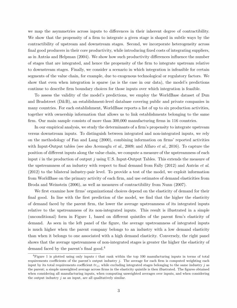
demand faced by the parent’s final good.4

4Figure 1 is plotted using only inputs i that rank within the top 100 manufacturing inputs in terms of totalrequirements coefficients of the parent’s output industry j. The average for each firm is computed weighting eachinput by its total requirements coefficient trij , while excluding integrated stages belonging to the same industry j asthe parent; a simple unweighted average across firms in the elasticity quintile is then illustrated. The figures obtainedwhen considering all manufacturing inputs, when computing unweighted averages over inputs, and when consideringthe output industry j as an input, are all qualitatively similar.

3

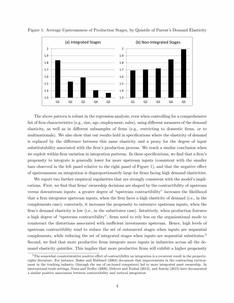
Figure 1: Average Upstreamness of Production Stages, by Quintile of Parent’s Demand Elasticity

(a) Integrated Stages (b) Non‐Integrated Stages

1.3

1.4

1.5

1.6

1.7

1.8

1.9

2

Q1 Q2 Q3 Q4 Q5

1.3

1.4

1.5

1.6

1.7

1.8

1.9

2

Q1 Q2 Q3 Q4 Q5

The above pattern is robust in the regression analysis, even when controlling for a comprehensive

list of firm characteristics (e.g., size, age, employment, sales), using different measures of the demand

elasticity, as well as in different subsamples of firms (e.g., restricting to domestic firms, or to

multinationals). We also show that our results hold in specifications where the elasticity of demand

is replaced by the difference between this same elasticity and a proxy for the degree of input

substitutability associated with the firm’s production process. We reach a similar conclusion when

we exploit within-firm variation in integration patterns. In these specifications, we find that a firm’s

propensity to integrate is generally lower for more upstream inputs (consistent with the smaller

bars observed in the left panel relative to the right panel of Figure 1), and that the negative effect

of upstreamness on integration is disproportionately large for firms facing high demand elasticities.

We report two further empirical regularities that are strongly consistent with the model’s impli-

cations. First, we find that firms’ ownership decisions are shaped by the contractibility of upstream

versus downstream inputs: a greater degree of “upstream contractibility” increases the likelihood

that a firm integrates upstream inputs, when the firm faces a high elasticity of demand (i.e., in the

complements case); conversely, it increases the propensity to outsource upstream inputs, when the

firm’s demand elasticity is low (i.e., in the substitutes case). Intuitively, when production features

a high degree of “upstream contractibility”, firms need to rely less on the organizational mode to

counteract the distortions associated with inefficient investments upstream. Hence, high levels of

upstream contractibility tend to reduce the set of outsourced stages when inputs are sequential

complements, while reducing the set of integrated stages when inputs are sequential substitutes.5

Second, we find that more productive firms integrate more inputs in industries across all the de-

mand elasticity quintiles. This implies that more productive firms will exhibit a higher propensity

5The somewhat counterintuitive positive effect of contractibility on integration is a recurrent result in the property-rights literature. For instance, Baker and Hubbard (2004) document that improvements in the contracting environ-ment in the trucking industry (through the use of on-board computers) led to more integrated asset ownership. Ininternational trade settings, Nunn and Trefler (2008), Defever and Toubal (2013), and Antras (2015) have documenteda similar positive association between contractibility and vertical integration.

4

to integrate relatively downstream (respectively, upstream) inputs when the elasticity of demand

for their final product is low (respectively, high); this is exactly what we uncover in the data.

This set of findings suggests that contractual frictions play a key role in shaping the integration

choices of firms around the world. The rich differential effects observed in the complements and

substitutes cases are consistent with a view of integration choices that is rooted in the property-

rights approach to the theory of the firm, though we do not rule out that these could possibly be

rationalized by alternative theories (as we briefly discuss in the concluding section). It is also useful

to describe how our analysis relates to other recent work on vertical linkages at the firm level. In

an influential study, Atalay et al. (2014) find little evidence of intrafirm shipments between related

plants within the United States; they instead present evidence indicating that firm boundaries

are more influenced by the transfer of intangible inputs, than by the transfer of physical goods.

Our theory is abstract enough to allow one to interpret the sequential investments as resulting in

either tangible or intangible transfers across establishments; and our empirical analysis takes into

account both manufacturing and non-manufacturing inputs (including services). That said, due

to the inherent difficulties in measuring intangible inputs, we believe that our empirical results

speak more to the optimal provision of incentives along sequential value chains involving tangible

inputs.6 Relatedly, our analysis suggests that intrafirm trade flows are an imperfect proxy for the

extent to which firms react to contractual insecurity by internalizing particular stages of their global

value chains. As the “sparse integration” extension of our model shows, internalization decisions

along value chains are consistent with an arbitrarily low level of intrafirm trade relative to the

overall transaction volume in these chains. This helps reconcile our findings with Ramondo et al.

(2016), who find intrafirm trade between U.S. multinationals and their affiliates abroad to be highly

concentrated among a small number of large affiliates.

Our work is closely related to two contemporaneous firm-level empirical investigations of the

Antras and Chor (2013) model. Del Prete and Rungi (2017) employ a dataset of about 4,000

multinational business groups to explore the correlation between the average “downstreamness”

of integrated affiliates and that of the parent firm itself (both measured relative to final demand).

Luck (2016) reports corroborating evidence based on the city-level value-chain position of processing

export activity in China. More generally, our paper is related to a recent empirical literature testing

various aspects of the property-rights theory of multinational firm boundaries.7

The remainder of the paper is organized as follows. Section 2 presents our model of firm

boundaries with sequential production and input asymmetries. Section 3 describes the data. Section

4 outlines our empirical methodology and presents our findings. Section 5 concludes. The Online

Appendix contains additional material related to both the theory and the empirical analysis.

6It is important to stress, however, that our findings should not be interpreted as invalidating the intangibleshypothesis. In fact, we will report some patterns in the data which are suggestive of an efficiency-enhancing role ofthe common ownership of proximate product lines.

7This includes Antras (2003), Yeaple (2006), Nunn and Trefler (2008, 2013), Corcos et al. (2013), Defever andToubal (2013), Dıez (2014), and Antras (2015), among others. Our work is also related to the broader empiricalliterature on firm boundaries; see Lafontaine and Slade (2007) and Bresnahan and Levin (2012) for overviews.

5

2 Theoretical Framework

In this section, we develop our model of sequential production. We first describe a generalized

version of the model in Antras and Chor (2013) that incorporates heterogeneity across inputs

beyond their position along the value chain. We then consider three extensions to derive additional

theoretical results and enrich the set of predictions that can be brought to the data.

2.1 Benchmark Model with Heterogeneous Inputs

We focus throughout on the problem of a firm seeking to optimally organize a manufacturing process

that culminates in a finished good valued by consumers. The final good is differentiated in the eyes

of consumers and belongs to a monopolistically competitive industry with a continuum of active

firms, each producing a differentiated variety. Consumer preferences over the industry’s varieties

feature a constant elasticity of substitution, so that the demand faced by the firm in question is:

q = Ap−1/(1−ρ), (1)

where A > 0 is a term that the firm takes as given, and the parameter ρ ∈ (0, 1) is positively

related to the degree of substitutability across final-good varieties. Note that A is allowed to vary

across firms in the industry (perhaps reflecting differences in quality), while the demand elasticity

1/ (1− ρ) is common for all firms in the sector. The latter assumption is immaterial for our

theoretical results, but will be exploited in the empirical implementation, where we rely on sectoral

estimates of demand elasticities. Given that we largely focus on the problem of a representative

firm, we abstain from indexing variables by firm or sector to keep the notation tidy.

Obtaining the finished product requires the completion of a unit measure of production stages.

These stages are indexed by i ∈ [0, 1], with a larger i corresponding to stages further downstream

and thus closer to the finished product. Denote by x(i) the value of the services of intermediate

inputs that the supplier of stage i delivers to the firm. Final-good production is then given by:

q = θ

(∫ 1

0(ψ (i)x(i))α I (i) di

)1/α

, (2)

where θ is a productivity parameter, α ∈ (0, 1) is a parameter that captures the (symmetric) degree

of substitutability among the stage inputs, the shifters ψ (i) reflect asymmetries in the marginal

product of different inputs’ investments, and I (i) is an indicator function that takes a value of 1

if input i is produced after all inputs i′ < i have been produced, and a value of 0 otherwise. The

technology in (2) resembles a conventional CES production function with a continuum of inputs,

but the indicator function I (i) makes the production technology inherently sequential.

Intermediate inputs are produced by a unit measure of suppliers, with the mapping between

inputs and suppliers being one-to-one. Inputs are customized to make them compatible with the

needs of the firm controlling the finished product. In order to provide a compatible input, the

6

supplier of input i must undertake a relationship-specific investment entailing a marginal cost of

c(i) per unit of input services x (i). All agents including the firm are capable of producing subpar

inputs at a negligible marginal cost, but these inputs add no value to final-good production apart

from allowing the continuation of the production process in situations in which a supplier threatens

not to deliver his or her input to the firm.

If the firm could discipline the behavior of suppliers via a comprehensive ex-ante contract, those

threats would be irrelevant. For instance, the firm could demand the delivery of a given volume

x (i) of input services in exchange for a fee, while including a clause in the contract that would

punish the supplier severely when failing to honor this contractual obligation. In practice, however,

a court of law will generally not be able to verify whether inputs are compatible or not. For the

time being, we will make the stark assumption that none of the aspects of input production can

be specified in a binding manner in an initial contract, except for a clause stipulating whether

the different suppliers are vertically integrated into the firm or remain independent. Because the

terms of exchange between the firm and the suppliers are not set in stone before production takes

place, the actual payment to a supplier (say the one controlling stage i) is negotiated bilaterally

only after the stage i input has been produced and the firm has had a chance to inspect it. At

that point, the firm and the supplier negotiate over the division of the incremental contribution to

total revenue generated by supplier i. The lack of an enforceable contract implies that suppliers

can set the volume of input services x (i) to maximize their payoff conditional on the value of the

semi-finished good they are handed by their immediate upstream supplier.

How does integration affect the game played between the firm and the unit measure of suppliers?

Following the property-rights theory of firm boundaries, we let the effective bargaining power of

the firm vis-a-vis a supplier depend on whether the firm owns this supplier. Under integration,

the firm controls the physical assets used in the production of the input, thus allowing the firm to

dictate a use of these assets that tilts the division of surplus in its favor. We capture this central

insight of the property-rights theory in a stark manner, with the firm obtaining a share βV of the

value of supplier i’s incremental contribution to total revenue when the supplier is integrated, while

receiving only a share βO < βV of that surplus when the supplier is a stand-alone entity.

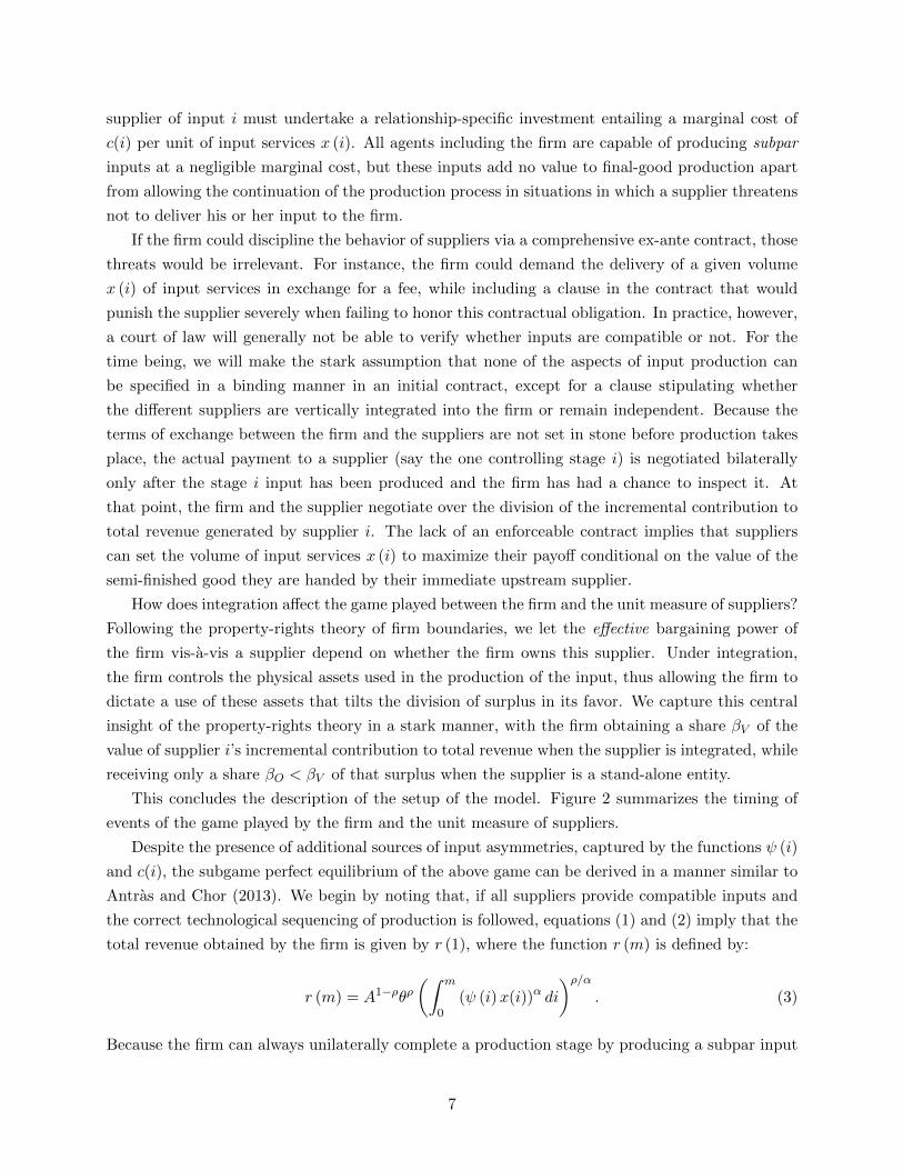
This concludes the description of the setup of the model. Figure 2 summarizes the timing of

events of the game played by the firm and the unit measure of suppliers.

Despite the presence of additional sources of input asymmetries, captured by the functions ψ (i)

and c(i), the subgame perfect equilibrium of the above game can be derived in a manner similar to

Antras and Chor (2013). We begin by noting that, if all suppliers provide compatible inputs and

the correct technological sequencing of production is followed, equations (1) and (2) imply that the

total revenue obtained by the firm is given by r (1), where the function r (m) is defined by:

r (m) = A1−ρθρ(∫ m

0(ψ (i)x(i))α di

)ρ/α. (3)

Because the firm can always unilaterally complete a production stage by producing a subpar input

7

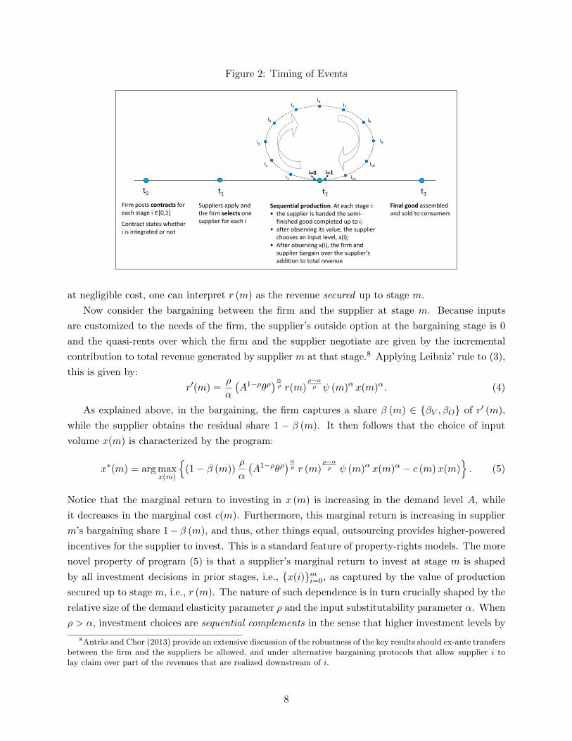
Figure 2: Timing of Events

i=0 t0 Firm posts contracts for each stage i ∈[0,1]

Contract states whether i is integrated or not

t3 Final good assembled and sold to consumers

t1

Suppliers apply and the firm selects one supplier for each i

t2

Sequential production. At each stage i: • the supplier is handed the semi-

finished good completed up to i; • after observing its value, the supplier

chooses an input level, x(i); • After observing x(i), the firm and

supplier bargain over the supplier’s addition to total revenue

i1 i2

i3

i4 i5

i6 i7 i8

i9

i10 i11 i=1

at negligible cost, one can interpret r (m) as the revenue secured up to stage m.

Now consider the bargaining between the firm and the supplier at stage m. Because inputs

are customized to the needs of the firm, the supplier’s outside option at the bargaining stage is 0

and the quasi-rents over which the firm and the supplier negotiate are given by the incremental

contribution to total revenue generated by supplier m at that stage.8 Applying Leibniz’ rule to (3),

this is given by:

r′(m) =ρ

α

(A1−ρθρ

)αρ r(m)

ρ−αρ ψ (m)α x(m)α. (4)

As explained above, in the bargaining, the firm captures a share β (m) ∈ βV , βO of r′ (m),

while the supplier obtains the residual share 1 − β (m). It then follows that the choice of input

volume x(m) is characterized by the program:

x∗(m) = arg maxx(m)

(1− β (m))

ρ

α

(A1−ρθρ

)αρ r (m)

ρ−αρ ψ (m)α x(m)α − c (m)x(m)

. (5)

Notice that the marginal return to investing in x (m) is increasing in the demand level A, while

it decreases in the marginal cost c(m). Furthermore, this marginal return is increasing in supplier

m’s bargaining share 1− β (m), and thus, other things equal, outsourcing provides higher-powered

incentives for the supplier to invest. This is a standard feature of property-rights models. The more

novel property of program (5) is that a supplier’s marginal return to invest at stage m is shaped

by all investment decisions in prior stages, i.e., x(i)mi=0, as captured by the value of production

secured up to stage m, i.e., r (m). The nature of such dependence is in turn crucially shaped by the

relative size of the demand elasticity parameter ρ and the input substitutability parameter α. When

ρ > α, investment choices are sequential complements in the sense that higher investment levels by

8Antras and Chor (2013) provide an extensive discussion of the robustness of the key results should ex-ante transfersbetween the firm and the suppliers be allowed, and under alternative bargaining protocols that allow supplier i tolay claim over part of the revenues that are realized downstream of i.

8

upstream suppliers increase the marginal return of supplier m’s own investment. Conversely, when

ρ < α, investment choices are sequential substitutes because high values of upstream investments

reduce the marginal return to investing in x(m). We shall refer to ρ > α as the complements case

and to ρ < α as the substitutes case, as in Antras and Chor (2013).

It is intuitively clear why low values of α will tend to render investments sequential complements.

Why might a low value of ρ render investments sequential substitutes? The reason for this is that

when ρ is low, the firm’s revenue function is highly concave in output and thus marginal revenue

falls at a relatively fast rate along the value chain. As a result, the incremental contribution to

revenue associated with supplier m – which is what the firm and supplier m bargain over – might

be particularly low when upstream suppliers have invested large amounts.

We now plug the first-order condition from (5) into (4), and solve the resulting separable differ-

ential equation. As shown in Section A-1 of the Online Appendix, one can express the equilibrium

volume of input m services x∗ (m) as a function of the whole path of bargaining shares β (i)i∈[0,m]

up to stage m:

x∗(m) = Aθρ

1−ρ

(1− ρ1− α

) ρ−αα(1−ρ)

ρ1

1−ρ

(1− β (m)

c (m)

) 11−α

ψ (m)α

1−α

[∫ m

0

((1− β (i))ψ (i)

c (i)

) α1−α

di

] ρ−αα(1−ρ)

.

(6)

It is then straightforward to see that x∗(m) > 0 for all m as long as β (m) < 1. This in turn

implies that the firm has every incentive to abide by the proper (or technological) sequencing of

production, so that I∗(m) = 1 for all m (consistent with our expressions above).

Next, we roll back to the initial period prior to any production taking place, in which the firm

decides whether the contract associated with a given input m is associated with integration or

outsourcing. This amounts to choosing β (i)i∈[0,1] to maximize πF =∫ 1

0 β(i)r′(i)di, with r′(m)

given in equation (4), x∗(m) in equation (6), and β (i) ∈ βV , βO. After several manipulations,

the problem of choosing the optimal organizational structure can be reduced to the program:

maxβ(i)

πF = Θ∫ 1

0 β(i)(

(1−β(i))ψ(i)c(i)

) α1−α

[∫ i0

((1−β(k))ψ(k)

c(k)

) α1−α

dk

] ρ−αα(1−ρ)

di

s.t. β (i) ∈ βV , βO ,

(7)

where Θ = Aθρ

1−ρ ρα

(1−ρ1−α

) ρ−αα(1−ρ)

ρρ

1−ρ > 0.

It will prove useful to consider a relaxed version of program (7) in which rather than constraining

β (i) to equal βV or βO, we allow the firm to freely choose the function β(i) from the whole set of

piecewise continuously differentiable real-valued functions. Defining:

v (i) ≡∫ i

0

((1− β (k))ψ (k)

c (k)

) α1−α

dk, (8)

we can then turn this relaxed program into a calculus of variation problem where the firm chooses

9

the real-value function v that maximizes:

πF (v) = Θ

∫ 1

0

(1− v′ (i)

1−αα

c (i)

ψ (i)

)v′ (i) v (i)

ρ−αα(1−ρ) di. (9)

In Section A-1 of the Online Appendix, we show that imposing the necessary Euler-Lagrange and

transversality conditions, and after a few cumbersome manipulations, the optimal (unrestricted)

division of surplus at stage m can be expressed as:

β∗ (m) = 1− α

[∫m0 (ψ (k) /c (k))

α1−α dk∫ 1

0 (ψ (k) /c (k))α

1−α dk

]α−ρα

. (10)

The term inside the square brackets is a monotonically increasing function of m. This confirms the

claim in Antras and Chor (2013) that whether the optimal division of surplus increases or decreases

along the value chain is shaped critically by the relative size of the parameters α and ρ.9 In the

complements case (ρ > α), the incentive to integrate suppliers increases as we move downstream

in the value chain. Intuitively, given sequential complementarity, the firm is particularly concerned

about incentivizing upstream suppliers to raise their investment effort, in order to generate positive

spillovers on the investment levels of downstream suppliers. Instead, in the substitutes case (ρ <

α), the firm is less concerned with underinvestment by upstream suppliers, while capturing rents

upstream is particularly appealing when marginal revenue falls quickly with output.

A remarkable feature of equation (10) is that the slope of ∂β∗ (m) /∂m is governed by the sign

of ρ − α regardless of the paths of ψ (k) and c (k). It is worth pausing to explain why this result

is not straightforward. Note that a disproportionately high value of ψ (m) at a given stage m can

be interpreted as that stage being relatively important in the production process.10 According to

one of the canonical results of the property-rights literature, one would then expect the incentive

to outsource such a stage to be particularly large (see, in particular, Proposition 1 in Antras,

2014). Intuitively, outsourcing provides higher-powered incentives to suppliers, and minimizing

underinvestment inefficiencies is particularly beneficial for inputs that are relatively important in

production. One might have thus expected the optimal division of surplus β∗ (m) to be decreasing

in stage m’s importance ψ (m). For the same reason, and given that input shares are monotonically

decreasing in the marginal cost c (m), one might have also expected the share β∗ (m) to be increasing

in c (m). One would then be led to conclude that if the path of ψ (m) were sufficiently increasing

in m – or the path of c (m) were sufficiently decreasing in m – then β∗ (m) would tend to decrease

along the value chain, particularly when the difference between ρ and α is small.

Equation (10) demonstrates, however, that this line of reasoning is flawed. No matter by how

little ρ and α differ, the slope of β∗ (m) is uniquely pinned down by the sign of ρ − α, regardless

9Although Antras and Chor (2013) considered a variant of their model with heterogeneity in ψ (i) and c (i), theyfailed to derive this explicit formula for β∗ (m) and simply noted that ∂β∗ (m) /∂m inherited the sign of ρ− α (see,in particular, equation (28) in their paper).

10Indeed, in a model with complete contracts, the share of m in the total input purchases of the firm would be amonotonically increasing function of ψ (m).

10

of the paths of ψ (m) and c (m). This result bears some resemblance to the classic result in

consumption theory that an agent’s dynamic utility-maximizing level of consumption should be

growing or declining over time according to whether the real interest rate is greater or smaller

than the rate of time preference, regardless of the agent’s income path. It is important to stress,

however, that the paths of ψ (m) and c (m) are not irrelevant for the incentive to integrate suppliers

along the value chain (in the same manner that the path of income is not irrelevant in the dynamic

consumption problem). Equation (10) illustrates that the incentives to integrate a particular input

will be notably shaped by the size of the ratio ψ (k) /c (k) for inputs upstream from input m relative

to the average size of this ratio along the whole value chain.

More specifically, in production processes featuring sequential complementarity, the higher is

the value of ψ (k) /c (k) for inputs upstream from m relative to its value for inputs downstream from

m, the higher will be the incentive of the firm to integrate stage m. The intuition behind this result

is as follows. Remember that when inputs are sequential complements, the marginal incentive of

supplier m to invest will be higher, the higher are the levels of investment by suppliers upstream

from m. Furthermore, fixing the ownership structure, these upstream investments will also tend to

be relatively large whenever stages m′ upstream from m are associated with disproportionately large

values of ψ (m′) or low values of c (m′). In those situations, and due to sequential complementarity,

the incentives to invest at stage m will also tend to be disproportionately large, and thus the

incentive of the firm to outsource stage m will be reduced relative to a situation in which the

ratio ψ (k) /c (k) is common for all stages. Conversely, whenever ρ < α, investments are sequential

substitutes, and thus high upstream investments related to disproportionately high upstream values

of ψ (m′) /c (m′) for m′ < m will instead increase the likelihood that stage m is outsourced.

So far, we have focused on a characterization of the optimal bargaining share β∗ (m), but the

above results can easily be turned into statements regarding the propensity of firms to integrate

(β∗ (m) = βV ) or outsource (β∗ (m) = βO) the different stages along the value chain. In particular,

in Section A-1 of the Online Appendix, we show that:

Proposition 1. In the complements case (ρ > α), there exists a unique m∗C ∈ (0, 1], such that:

(i) all production stages m ∈ [0,m∗C) are outsourced; and (ii) all stages m ∈ [m∗C , 1] are integrated

within firm boundaries. In the substitutes case (ρ < α), there exists a unique m∗S ∈ (0, 1], such

that: (i) all production stages m ∈ [0,m∗S) are integrated within firm boundaries; and (ii) all stages

m ∈ [m∗S , 1] are outsourced. Furthermore, both m∗C and m∗S are lower, the higher is the ratio

ψ (m) /c (m) for upstream inputs relative to downstream inputs.

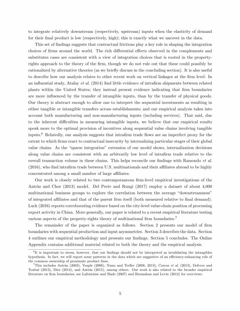
Figure 3 illustrates the main result in Proposition 1 concerning the optimal pattern of ownership

along the value chain. When the demand faced by the final-good producer is sufficiently elastic,

then there exists a unique cutoff stage such that all inputs prior to that cutoff are outsourced, and

all inputs (if any) downstream of it are integrated. The converse prediction holds when demand

is sufficiently inelastic (i.e., in the sequential substitutes case): the firm would instead integrate

relatively upstream inputs, while outsourcing would take place relatively downstream.

Although the last statement in Proposition 1 follows pretty immediately from our discussion of

11

Figure 3: Firm Boundary Choices along the Value Chain

0 1

Outsource Integrate

Sequential complements:

0 1

OutsourceIntegrate

Sequential substitutes:

mC* mS*

the properties of the solution β∗ (m) to the relaxed problem, it can also be shown more directly

by explicitly characterizing the thresholds m∗C and m∗S . For the sequential complements case, we

show in Section A-1 of the Online Appendix that, provided that integration and outsourcing coexist

along the value chain, the threshold m∗C is given by:

∫m∗C

0 (ψ (k) /c (k))α

1−α dk∫ 10 (ψ (k) /c (k))

α1−α dk

=

1 +

(1− βO1− βV

) α1−α

1− βO

βV

1−(

1−βO1−βV

)− α1−α

α(1−ρ)ρ−α

− 1

−1

. (11)

Notice then that the larger the value of ψ (k) /c (k) in upstream production stages (in the numerator

of the left-hand side) relative to downstream production stages, the lower will be the value of m∗C ;

the set of integrated stages will thus be larger.11 (The analogous expression for m∗S in the substitutes

case is reported in Section A-1 of the Online Appendix.)

2.2 Extensions

A. Heterogeneous Contractibility of Inputs

In order to develop empirical tests of Proposition 1 – and especially its last statement – it is

important to map variation in the ratio ψ (m) /c (m) along the value chain to certain observables.

With that in mind, in this section we explore the link between ψ (m) and the degree of contractibility

of different stage inputs. In Section A-1 of the Online Appendix, we also briefly relate marginal

cost variation in c (m) along the value chain to the sourcing location decisions of the firm.12

Remember that in our benchmark model, x (m) captures the services related to the non-

contractible aspects of input production, in the sense that the volume x (m) cannot be disciplined

via an initial contract and is chosen unilaterally by suppliers. Conversely, we shall now assume

that ψ (m) encapsulates investments and other aspects of production that are specified in the ini-

tial contract in a way that precludes any deviation from that agreed level. In light of equation (2),

11In the complements case, integration and outsourcing coexist along the value chain when βV (1 − βV )α

1−α >

βO (1 − βO)α

1−α , which ensures m∗C < 1. When instead βV (1 − βV )

α1−α < βO (1 − βO)

α1−α , the firm finds it optimal

to outsource all stages, i.e., m∗C = 1.

12In the absence of contractual frictions, ψ (m) /c (m) would be positively related to the relative use of input m inthe production of the firm’s good, and one could presumably use information from Input-Output tables to constructempirical proxies for this ratio. Unfortunately, such a mapping between ψ (m) /c (m) and input m’s share in the totalinput purchases of firms is blurred by incomplete contracting and sequential production.

12

our assumptions imply that input production is a symmetric Cobb-Douglas function of contractible

and non-contractible aspects of production. To capture differential contractibility along the value

chain, we let stages differ in the (legal) costs associated with specifying these contractible aspects

of production. More specifically, we denote these contracting costs by (ψ (m))φ /µ (m) per unit of

ψ (m). We shall refer to µ (m) as the level of contractibility of stage m.13 The parameter φ > 1

captures the intuitive notion that it becomes increasingly costly to render additional aspects of

production contractible. We shall assume that the firm bears the full cost of these contractible

investments (perhaps by compensating suppliers for them upfront), but our results would not be

affected if the firm bore only a fraction of these costs. To simplify matters, we let the marginal cost

c (m) of non-contractible investments be constant along the value chain, i.e., c (m) = c for all m.

In terms of the timing of events summarized in Figure 2, notice that nothing has changed except

for the fact that the initial contract also specifies the profit-maximizing choice of ψ (m) along the

value chain. Furthermore, once the levels of ψ (m) have been set at stage t0, the subgame perfect

equilibrium is identical to that in our previous model in which ψ (m) was assumed exogenous. This

implies that the firm’s optimal ownership structure along the value chain will seek to maximize the

program in (7), and the solution of this problem will be characterized by Proposition 1.

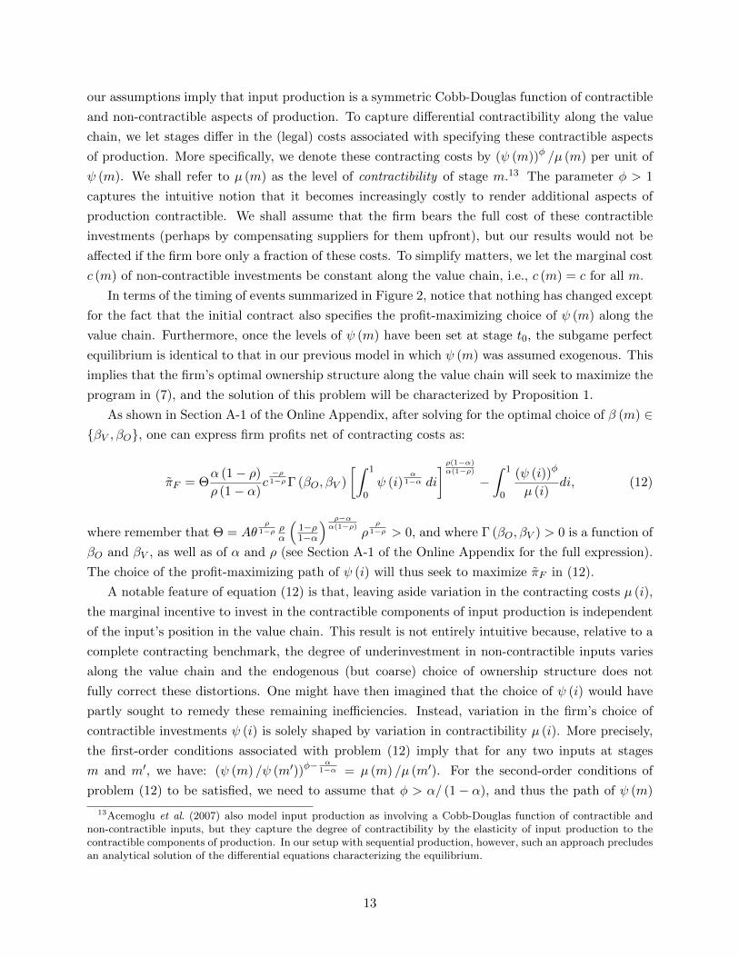
As shown in Section A-1 of the Online Appendix, after solving for the optimal choice of β (m) ∈βV , βO, one can express firm profits net of contracting costs as:

πF = Θα (1− ρ)

ρ (1− α)c

−ρ1−ρΓ (βO, βV )

[∫ 1

0ψ (i)

α1−α di

] ρ(1−α)α(1−ρ)

−∫ 1

0

(ψ (i))φ

µ (i)di, (12)

where remember that Θ = Aθρ

1−ρ ρα

(1−ρ1−α

) ρ−αα(1−ρ)

ρρ

1−ρ > 0, and where Γ (βO, βV ) > 0 is a function of

βO and βV , as well as of α and ρ (see Section A-1 of the Online Appendix for the full expression).

The choice of the profit-maximizing path of ψ (i) will thus seek to maximize πF in (12).

A notable feature of equation (12) is that, leaving aside variation in the contracting costs µ (i),

the marginal incentive to invest in the contractible components of input production is independent

of the input’s position in the value chain. This result is not entirely intuitive because, relative to a

complete contracting benchmark, the degree of underinvestment in non-contractible inputs varies

along the value chain and the endogenous (but coarse) choice of ownership structure does not

fully correct these distortions. One might have then imagined that the choice of ψ (i) would have

partly sought to remedy these remaining inefficiencies. Instead, variation in the firm’s choice of

contractible investments ψ (i) is solely shaped by variation in contractibility µ (i). More precisely,

the first-order conditions associated with problem (12) imply that for any two inputs at stages

m and m′, we have: (ψ (m) /ψ (m′))φ−α

1−α = µ (m) /µ (m′). For the second-order conditions of

problem (12) to be satisfied, we need to assume that φ > α/ (1− α), and thus the path of ψ (m)

13Acemoglu et al. (2007) also model input production as involving a Cobb-Douglas function of contractible andnon-contractible inputs, but they capture the degree of contractibility by the elasticity of input production to thecontractible components of production. In our setup with sequential production, however, such an approach precludesan analytical solution of the differential equations characterizing the equilibrium.

13

along the value chain is inversely related to the path of the exogenous contracting costs 1/µ (m).14

In light of our discussion in the last section, this implies:

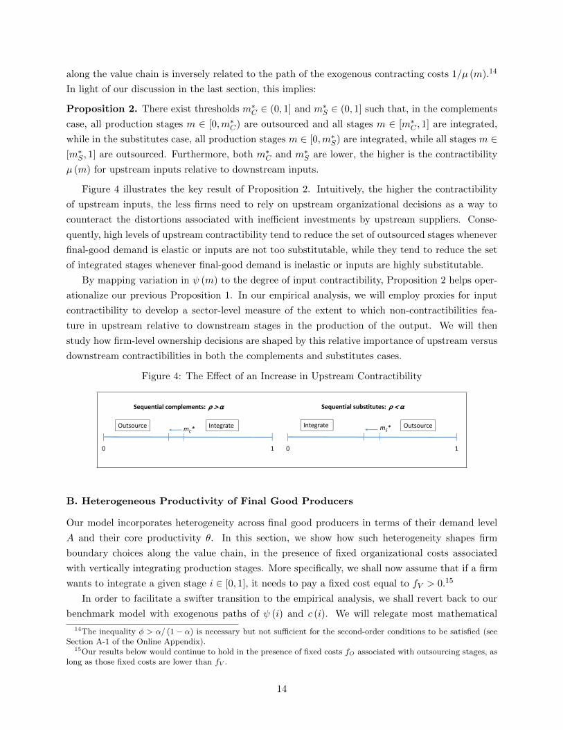
Proposition 2. There exist thresholds m∗C ∈ (0, 1] and m∗S ∈ (0, 1] such that, in the complements

case, all production stages m ∈ [0,m∗C) are outsourced and all stages m ∈ [m∗C , 1] are integrated,

while in the substitutes case, all production stages m ∈ [0,m∗S) are integrated, while all stages m ∈[m∗S , 1] are outsourced. Furthermore, both m∗C and m∗S are lower, the higher is the contractibility

µ (m) for upstream inputs relative to downstream inputs.

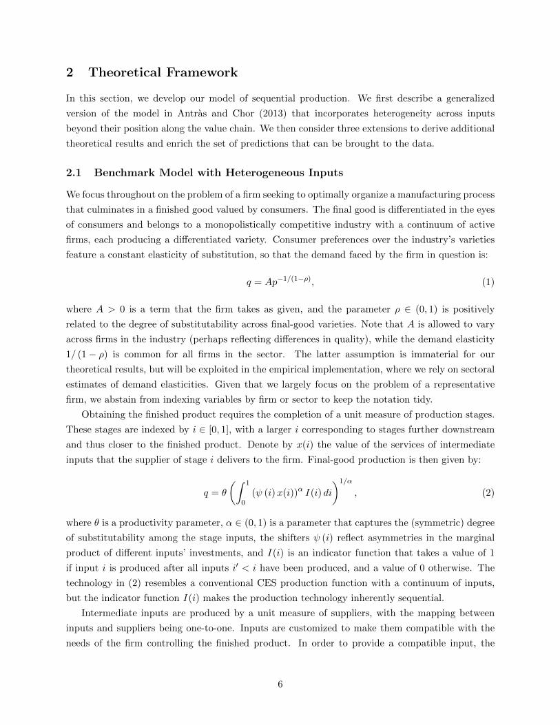
Figure 4 illustrates the key result of Proposition 2. Intuitively, the higher the contractibility

of upstream inputs, the less firms need to rely on upstream organizational decisions as a way to

counteract the distortions associated with inefficient investments by upstream suppliers. Conse-

quently, high levels of upstream contractibility tend to reduce the set of outsourced stages whenever

final-good demand is elastic or inputs are not too substitutable, while they tend to reduce the set

of integrated stages whenever final-good demand is inelastic or inputs are highly substitutable.

By mapping variation in ψ (m) to the degree of input contractibility, Proposition 2 helps oper-

ationalize our previous Proposition 1. In our empirical analysis, we will employ proxies for input

contractibility to develop a sector-level measure of the extent to which non-contractibilities fea-

ture in upstream relative to downstream stages in the production of the output. We will then

study how firm-level ownership decisions are shaped by this relative importance of upstream versus

downstream contractibilities in both the complements and substitutes cases.

Figure 4: The Effect of an Increase in Upstream Contractibility

0 1

Outsource Integrate

Sequential complements:

0 1

OutsourceIntegrate

Sequential substitutes:

mC* mS*

B. Heterogeneous Productivity of Final Good Producers

Our model incorporates heterogeneity across final good producers in terms of their demand level

A and their core productivity θ. In this section, we show how such heterogeneity shapes firm

boundary choices along the value chain, in the presence of fixed organizational costs associated

with vertically integrating production stages. More specifically, we shall now assume that if a firm

wants to integrate a given stage i ∈ [0, 1], it needs to pay a fixed cost equal to fV > 0.15

In order to facilitate a swifter transition to the empirical analysis, we shall revert back to our

benchmark model with exogenous paths of ψ (i) and c (i). We will relegate most mathematical

14The inequality φ > α/ (1 − α) is necessary but not sufficient for the second-order conditions to be satisfied (seeSection A-1 of the Online Appendix).

15Our results below would continue to hold in the presence of fixed costs fO associated with outsourcing stages, aslong as those fixed costs are lower than fV .

14

details to Section A-1 of the Online Appendix, in which we show that Proposition 1 continues

to apply in this environment with fixed costs of integration. More precisely, there continue to

exist thresholds m∗C ∈ (0, 1] and m∗S ∈ (0, 1] such that all production stages m ∈ [0,m∗C) are

outsourced and all stages m ∈ [m∗C , 1] are integrated in the complements case, while all production

stages m ∈ [0,m∗S) are integrated and all stages m ∈ [m∗S , 1] are outsourced in the substitutes case.

Furthermore, one can still show that both m∗C and m∗S are lower, the higher is the ratio ψ (m) /c (m)

for upstream inputs relative to downstream inputs. These characterization results can be obtained

even though the equations determining the cutoffs m∗C and m∗S are now significantly more involved.

More relevant for the purposes of this section, the equilibrium conditions defining m∗C and m∗Scan also be used to study how these thresholds are affected by changes in A and θ. In Section A-1

of the Online Appendix, we show that m∗C is necessarily a decreasing function of the level of firm

demand A or firm productivity θ. By contrast, m∗S is increasing in both A and θ. In words, this

implies that regardless of the sign of ρ− α, relatively more productive firms will tend to integrate

a larger interval of production stages. The intuition behind this is simple: more productive firms

find it easier to amortize the fixed cost associated with integrating more stages.

In our empirical analysis, we will explore whether the observed intra-industry heterogeneity in

integration choices is in accordance with these predictions, which we summarize as:

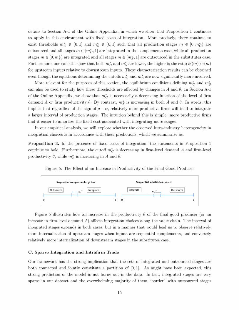
Proposition 3. In the presence of fixed costs of integration, the statements in Proposition 1

continue to hold. Furthermore, the cutoff m∗C is decreasing in firm-level demand A and firm-level

productivity θ, while m∗S is increasing in A and θ.

Figure 5: The Effect of an Increase in Productivity of the Final Good Producer

0 1

Outsource Integrate

Sequential complements:

0 1

OutsourceIntegrate

Sequential substitutes:

mC* mS*

Figure 5 illustrates how an increase in the productivity θ of the final good producer (or an

increase in firm-level demand A) affects integration choices along the value chain. The interval of

integrated stages expands in both cases, but in a manner that would lead us to observe relatively

more internalization of upstream stages when inputs are sequential complements, and conversely

relatively more internalization of downstream stages in the substitutes case.

C. Sparse Integration and Intrafirm Trade

Our framework has the strong implication that the sets of integrated and outsourced stages are

both connected and jointly constitute a partition of [0, 1]. As might have been expected, this

strong prediction of the model is not borne out in the data. In fact, integrated stages are very

sparse in our dataset and the overwhelming majority of them “border” with outsourced stages

15

immediately upstream and downstream from them.16 This paucity of integration might be due to

technological or regulatory factors that make vertical integration infeasible for certain production

stages. We next briefly outline a third extension of our model that accommodates such sparsity,

and we demonstrate that it does not undermine the validity of the key predictions of the model

that we will take to the data.

A simple way to render integration infeasible for certain segments of the value chain is to

assume that the fixed costs of integrating those segments is arbitrarily large. In terms of our

second extension above, we thus now have that the fixed cost of integration is stage-specific and

takes a value of fV (m) = +∞ for any m ∈ Υ, where Υ is the set of stages that cannot possibly

be integrated. For simplicity, we assume that the fixed costs of integration are finite and identical

for all remaining stages, so fV (m) = fV for m ∈ Ω, where Ω is the set of integrable stages (i.e.,

Ω = [0, 1] \Υ). Clearly, by making the set Υ larger and larger, one can make integration decisions

arbitrarily sparse in our model. As we show in Section A-1 of the Online Appendix, despite the

presence of the exogenously non-integrable stages, we can establish that:

Proposition 4. If ρ > α, the firm cannot possibly find it optimal to integrate a positive measure

of stages located upstream from a positive measure of outsourced stages (m, m+ ε) ∈ Ω that could

have been integrated. If ρ < α, the firm cannot possibly find it optimal to integrate a positive

measure of stages located downstream from a positive measure of outsourced stages (m, m+ε) ∈ Ω

that could have been integrated.

Naturally, Proposition 4 provides a much weaker characterization of the integration decisions

of firms along their value chain than our previous Propositions 1-3. Yet, a corollary of Proposition

4 is that, holding constant the set Υ of stages that cannot possibly be integrated, the average

upstreamness of integrated stages relative to the average upstreamness of outsourced stages should

be lower when ρ > α than when ρ < α. This relative upstreamness of integrated and non-integrated

stages is what we refer to as “ratio-upstreamness” in our regression analysis, and will be one of the

key metrics employed to assess the empirical validity of the model.

An interesting implication of the sparsity of integrated stages in the value chain is that, as

the set Υ expands, the volume of intrafirm trade in the value chain becomes smaller and smaller.

Intuitively, in such a case, each interval of integrated stages becomes increasingly isolated, and

necessarily trades at arm’s length with their immediate “neighbors” in the value chain. This

confirms our claim in the Introduction that in sequential production processes in which physical

goods flow through both integrated and non-integrated plants, and in which the former are largely

outnumbered by the latter, the volume of intrafirm trade flows may be a poor proxy of the extent

to which firms’ integration decisions are shaped by contractual incompleteness.

16For our full sample of firms, the median number of integrated stages is 2, while the median number of non-integrated stages – i.e., all inputs with positive total requirements coefficients – is 906. When restricting the sampleto the top 100 manufacturing inputs ranked by the total requirements coefficients of the associated output industry,0.11 percent of all integrated stages are immediately preceded or succeeded by another integrated stage. The nextsection discusses in detail how we identify integrated and non-integrated stages, and their position in the value chain.

16

3 Dataset and Key Variables

We turn now to our empirical analysis. To assess the validity of our model, we need firm-specific

information on integrated and outsourced inputs, as well as a measure of the “upstreamness” of

these various inputs. We also require proxies for whether a whether a final-good industry falls into

the complements or substitutes case, and a measure of input contractibility. In this section, we

describe the dataset that we employ, together with the construction of these key variables.

3.1 The WorldBase Dataset

Our core firm-level dataset is Dun & Bradstreet’s (D&B) WorldBase, which provides comprehensive

coverage of public and private companies across more than 100 countries and territories. WorldBase

has been used extensively in the literature, in particular to explore research questions related to

the organizational practices of firms around the world.17,18

A key advantage of WorldBase is that the unit of observation is the establishment, namely a

single physical location where industrial operations or services are performed, or business is con-

ducted. Each establishment in WorldBase is assigned a unique identifier, called a DUNS number.19

Where applicable, the DUNS number of the global ultimate owner is also reported, which allows

us to keep track of ownership linkages within the dataset. In addition, WorldBase provides infor-

mation on: (i) the location (address) of each establishment; (ii) the 4-digit SIC code (1987 version)

of its primary industry, and the SIC codes of up to five secondary industries; (iii) the year it was

started or in which current ownership took control; and (iv) basic data on employment and sales.

Note that each firm in the data is either: (i) a single-establishment; or (ii) is identified in World-

Base as a “global ultimate”. The former refers to a business entity whose entire activity is in one

location, and which does not report ownership links with other establishments in WorldBase. For

the latter, D&B WorldBase defines a “global ultimate” to be the top, most important, responsible

entity within a corporate family tree, that has more than 50% ownership of other establishments.

We link each global ultimate to all its identified majority-owned subsidiaries, both in manufactur-

ing and non-manufacturing, by using the DUNS number of the global ultimate that is reported for

establishments. The set of integrated SIC activities for a single-establishment is simply the list of

up to six SIC codes associated with it. The set of integrated SIC codes for a global ultimate is the

complete list of SIC activities that is performed either in its headquarters or one of its subsidiaries.

Moving forward, we will refer simply to each observation as a “parent” firm, indexed by p.

For our analysis, we use the 2004/2005 WorldBase vintage and focus on parent firms in the man-

ufacturing sector – i.e., whose primary SIC code lies between 2000 and 3999 – with a minimum total

17Recent uses include Acemoglu et al. (2009), Alfaro and Charlton (2009), Alfaro and Chen (2014), Fajgelbaum etal. (2015), and Alfaro et al. (2016).

18The data in WorldBase is compiled from a large number of sources, including business registers, company websites,and self-registration. See Alfaro and Charlton (2009) for a detailed discussion, and comparisons with other datasets.

19D&B uses the U.S. Standard Industrial Classification Manual 1987 edition to classify business establishments.The Data Universal Numbering System – the D&B DUNS Number – supports the linking of plants and firms acrosscountries, and tracking of plants’ histories including name changes.

17

employment (across all establishments) of 20. To be clear, while each parent firm in our sample has

a primary SIC code in manufacturing, we nevertheless include all the parent firm’s integrated SIC

activities (both in manufacturing and non-manufacturing) in the exercise that follows. In all, our

sample contains 320,254 parent firms from 116 countries; 259,312 of these are single-establishment

firms, while 60,942 are global ultimates. Among the global ultimates, 6,370 observations have

subsidiaries in more than one country, and are thus multinational firms. Panel A of Table A-1 in

the Online Appendix provides descriptive statistics for our full sample, as well as for the subset

of multinationals. Not surprisingly, multinationals are on average larger in terms of employment,

sales and number of integrated SIC codes, as compared to the typical firm in our data. We will

show nevertheless that our core findings concerning the relationship between “upstreamness” and

integration patterns are stable when we look at different subsamples.

3.2 Key Variables

We describe below the dependent variable and the key industry controls used in our analysis.

Descriptive statistics for these controls are provided in Table A-2 in the Online Appendix.

Integrated and Outsourced Inputs. For each parent, WorldBase provides us with infor-

mation on the inputs that are integrated within the firm’s ownership boundaries. In order to

further identify which inputs are outsourced, we combine the above with information from U.S.

Input-Output (I-O) Tables, following the methodology of Fan and Lang (2000).

Consider an economy with N > 1 industries. We refer to output industries by j and input

industries by i. For each industry pair, the I-O Tables report the dollar value of i used directly

as an input in the production of $1 of j, also known as the direct requirements coefficient, drij ;

denote with D the square matrix that has drij as its (i, j)-th entry. In practice, each input i can be

used not just directly, but could also enter further upstream, i.e., more than one stage prior to the

actual production of j. The total dollar value of i used either directly or indirectly to produce $1

of j is the total requirements coefficient, trij . As is well known, trij is given by the (i, j)-th entry

of [I −D]−1D, where I is the identity matrix and [I −D]−1 is the Leontief inverse matrix.

In our baseline analysis, we designate the primary SIC code reported in WorldBase for each

parent p as its output industry j. We first use the I-O Tables to deduce the set of 4-digit SIC inputs

S(j) – including both manufacturing and non-manufacturing inputs – that are used either directly

or indirectly in the production of j, namely: S(j) = i : trij > 0. We identify which inputs are

integrated and which are outsourced as follows. Define I(p) ⊆ S(j) to be the set of integrated

inputs of parent p. The elements of I(p) are the primary and secondary SIC codes of p and all its

subsidiaries (if any) as reported in WorldBase, these being inputs that the parent can in principle

obtain within its ownership boundaries. We then define the complement set, NI(p) = S(j) \ I(p),

to be the set of non-integrated SICs for parent p, these being the inputs required in the production

of j that have not been identified as integrated in I(p). Note that with this construction, the

primary SIC activity j of the parent is automatically classified as an element of I(p), so we will

later explore the robustness of our results to dropping this “self-SIC” code. (We will also consider

18

several alternative treatments of what constitutes the output industry j for those parent firms that

feature multiple manufacturing SIC codes.)

To implement the above, we turn to the 1992 U.S. Benchmark I-O Tables from the Bureau of

Economic Analysis (BEA). The U.S. Tables are one of the few publicly-available I-O accounts that

provide a level of industry detail close to the 4-digit SIC codes used in WorldBase, while the 1992

vintage is the most recent year for which the BEA provides a concordance from its I-O industry

classification to the 1987 SIC system.20 Readers familiar with these tables will be aware that the

concordance is not a one-to-one key. This is not a major problem given our focus on parents whose

primary output j is in manufacturing, as the key assigns a unique 6-digit I-O industry to each

4-digit SIC code between 2000 and 3999. Outside these sectors, in those inputs i whose 6-digit I-O

industry code maps to multiple 4-digit SIC codes, we split the total requirements value trij equally

across the multiple SIC codes that i maps to.

Panel A of Table A-1 in the Online Appendix shows that the mean trij value associated with

the inputs integrated by firms in WorldBase is 0.019241 (or 0.006774 when the I-O diagonal entries

are dropped); this is larger than the average trij value across the 416,349 (i, j) pairs in the I-O

Tables that are relevant to our study (0.001311). In other words, firms tend to integrate stages that

are more important in terms of total requirements usage.21 Moreover, 98.0% of the (i, j) pairs in

our WorldBase sample, namely inputs i that are integrated by a parent firm with output industry

j, are relevant for production in the sense that trij > 0.22 As mentioned before, firms tend to

integrate very few of the inputs necessary to produce their final good. The median number of

integrated stages is 2, compared to a median number of non-integrated stages equal to 906. There

is considerable skewness, as the corresponding 90th, 95th, and 99th percentiles of the number of

integrated stages are 3, 4, and 6, while the maximum number is 254.23 As discussed below, however,

integrated inputs tend to be “bunched” together along the value chain, consistent with our model.

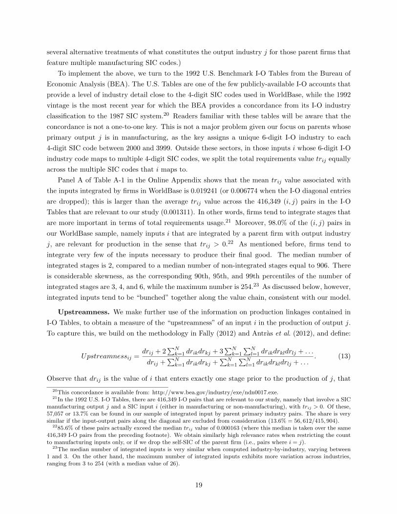
Upstreamness. We make further use of the information on production linkages contained in

I-O Tables, to obtain a measure of the “upstreamness” of an input i in the production of output j.

To capture this, we build on the methodology in Fally (2012) and Antras et al. (2012), and define:

Upstreamnessij =drij + 2

∑Nk=1 drikdrkj + 3

∑Nk=1

∑Nl=1 drikdrkldrlj + . . .

drij +∑N

k=1 drikdrkj +∑N

k=1

∑Nl=1 drikdrkldrlj + . . .

. (13)

Observe that drij is the value of i that enters exactly one stage prior to the production of j, that

20This concordance is available from: http://www.bea.gov/industry/exe/ndn0017.exe.21In the 1992 U.S. I-O Tables, there are 416,349 I-O pairs that are relevant to our study, namely that involve a SIC

manufacturing output j and a SIC input i (either in manufacturing or non-manufacturing), with trij > 0. Of these,57,057 or 13.7% can be found in our sample of integrated input by parent primary industry pairs. The share is verysimilar if the input-output pairs along the diagonal are excluded from consideration (13.6% = 56, 612/415, 904).

2285.6% of these pairs actually exceed the median trij value of 0.000163 (where this median is taken over the same416,349 I-O pairs from the preceding footnote). We obtain similarly high relevance rates when restricting the countto manufacturing inputs only, or if we drop the self-SIC of the parent firm (i.e., pairs where i = j).

23The median number of integrated inputs is very similar when computed industry-by-industry, varying between1 and 3. On the other hand, the maximum number of integrated inputs exhibits more variation across industries,ranging from 3 to 254 (with a median value of 26).

19

∑Nk=1 drikdrkj is the value of i that enters two stages prior to production of j, and so on and so

forth. The denominator in (13) is therefore equal to trij , written as an infinite sum over the value of

i’s use that enters exactly n stages removed from the production of j (where n = 1, 2, . . . ,∞). The

numerator is similarly an infinite sum, but there each input use term is multiplied by an integer

equal to the number of stages upstream at which the input value enters the production process.

Looking then at (13), Upstreamnessij is a weighted average of how many stages removed from j

the use of i is, where the weights correspond to the share of trij that enters at that corresponding

upstream stage. In particular, a larger Upstreamnessij means that a greater share of the total input

use value of i is accrued further upstream in the production process for j.

Note that Upstreamnessij ≥ 1 by construction, with equality if and only if trij = drij , namely

when the entirety of the input use of i goes directly into the production of j via one stage. With

some matrix algebra, one can see that the numerator of (13) is equal to the (i, j)-th entry of

[I−D]−2D. Together with the formula for trij noted earlier (i.e., the (i, j)-th entry of [I−D]−1D),

one can then calculate Upstreamnessij when provided with the direct requirements matrix. We

should stress the distinction between Upstreamnessij and the measure put forward in Fally (2012)

and Antras et al. (2012). The measure in this earlier work captured the average production line

position of each industry i with respect to final demand (i.e., consumption and investment), whereas

our current Upstreamnessij instead reflects the position of input i with respect to output industry

j, and is therefore a measure of production staging specific to each input-output industry pair.24

We use the direct requirements matrix derived from the 1992 U.S. I-O Tables to calculate

Upstreamnessij .25 We first obtain Upstreamnessij for each 6-digit I-O industry pair, before mapping

these to 4-digit SIC codes. As mentioned earlier, each 4-digit manufacturing SIC code is mapped

to a single 6-digit I-O code; this means that we can uniquely assign an Upstreamnessij value to SIC

code pairs where both the input i and output j are in manufacturing. The complications arise only

when we have a non-manufacturing input i which maps to multiple 6-digit I-O codes. For such

cases, we take a simple mean of Upstreamnessij over the constituent I-O codes of the SIC input

industry.26 To be clear, what this yields is a measure of the average number of production stages

based on the I-O classification system that are traversed between a given pair of SIC industries.

Panel B of Table A-1 in the Online Appendix presents some basic information on Upstreamnessij

after the mapping to SIC codes. There, we also illustrate in Figure A-1 the rich variation in this

measure, using one particular input industry, Tires and Inner Tubes (SIC 3011).

24The Upstreamnessij measure also has the interpretation of an “average propagation length”, this being a conceptintroduced in Dietzenbacher et al. (2005) to capture the average number of stages taken by a shock in i to spread toindustry j. Dietzenbacher et al. (2005) show that this average propagation length has the appealing property that itis invariant to whether one adopts a forward or backward linkage perspective when computing the average numberof stages between a pair of industries.

25We apply an open-economy and net-inventories correction to the direct requirements matrix D, before calculatingtrij and Upstreamnessij . This involves a simple adjustment to each drij to take into account input flows across borders,as well as into and out of inventories, on the assumption that these flows occur in proportion to what is observed indomestic input-output transactions; see Antras et al. (2012) for details.

26We have obtained very similar results under alternative approaches, including: using the median value; taking arandom pick; or using the trij-weighted average value.

20

As noted before, firms tend to integrate few inputs. This is a key feature of the data that our

model can accommodate, as explained in the discussion on “sparse integration” in Section 2.2.C.

Our upstreamness measure allows us to examine the extent to which – though sparse – integrated

inputs nevertheless tend to be “bunched” together, consistent with the environment described in

this earlier extension on “sparse integration”. To do so, we focus on firms that report at least

two secondary manufacturing SIC codes (on top of their primary output industry j). Table A-

3 in the Online Appendix computes the probability that a pair of randomly drawn integrated

manufacturing SICs of a given firm would belong to any two quintiles of Upstreamnessij , where

the quintiles are taken over all SIC manufacturing inputs i in the value chain for producing j; the

reported probability is an average across all firms under consideration. From Table A-3, one can see

that firms are clearly more likely to integrate inputs in the first quintile of upstreamness than in the

other quintiles. Leaving aside this first quintile, note that the probability that a firm integrates an

input is significantly higher when it already owns an input in the same quintile, and furthermore

these probabilities fall for quintiles that are further apart. These patterns are suggestive of the

existence of “bunching” along the value chain in the integration decisions of firms.

Ratio-Upstreamness. To test whether the variation across parent firms in integration deci-

sions is consistent with our theory, we first explore specifications with a dependent variable that

summarizes the extent to which a firm’s integrated inputs tend to be more upstream compared to

its non-integrated inputs. For this purpose, we construct the following measure for each parent:

Ratio-Upstreamnessjp =

∑i∈I(p) θ

IijpUpsteamnessij∑

i∈NI(p) θNIijpUpstreamnessij

, (14)

where θIijp = trij/∑

i∈I(p) trij and θNIijp = trij/∑

i∈NI(p) trij . This takes the ratio of a weighted-

average upstreamness of p’s integrated inputs relative to that of its non-integrated inputs; the

weights are proportional to the total requirements coefficients to capture the relative importance of

each input in the production of j. Ratio-Upstreamnessjp is thus larger, the greater the propensity

of p to integrate relatively upstream inputs, while outsourcing more downstream inputs.

We will consider several alternative constructions of Ratio-Upstreamnessjp to assess the robust-

ness of our results. These include: (i) restricting S(j) to the set of “ever-integrated” inputs, namely

inputs i for which we actually observe at least one parent in industry j that integrates i within its

boundaries; (ii) restricting S(j) to the set of manufacturing inputs; and (iii) excluding the self-SIC

from S(j). The first alternative measure of Ratio-Upstreamnessjp is of particular importance. The

restriction to the set of “ever-integrated” inputs is a plausible criterion for removing input-output

industry pairs for which the fixed costs of integration are prohibitively high. By constructing Ratio-

Upstreamnessjp using only the subset of inputs for which integration is seen in our dataset to be

feasible, we are able to test more closely the predictions of the model that arise in the empirically-

relevant case where integrated inputs are sparse (i.e., Proposition 4). Panel C of Table A-1 in the

Online Appendix presents summary statistics for the different ratio-upstreamness measures.

Our first set of regression specifications will use Ratio-Upstreamnessjp as the dependent variable,

21

and thus seek to exploit the variation across firms in this measure. Our theory has predictions at

the input level as well, so we will also present evidence based on variation within firms in integration

decisions across inputs. For this second set of specifications, we adopt as the dependent variable a

0-1 indicator for whether the input in question is integrated within the parent’s ownership structure,

i.e., whether i ∈ I(p). In both the cross- and within-firm exercises, we will present evidence based

on a broad set of inputs used in production by the firms, as well as when restricting to the subset

of ever-integrated inputs to account for the sparsity of integrated stages.

Our dataset does not allow us to directly observe whether plants that are related in an ownership

sense actually contribute inputs and components to a common production process. It is important

to stress that any potential misclassification of integrated versus non-integrated inputs (in the sets

I(p) and NI(p)) would give rise to measurement error in the dependent variable in our regressions.

To the extent that this is classical measurement error, it would make our coefficient estimates less

precise, making it harder to find empirical support for the model’s predictions.

Demand Elasticity. As highlighted in our theory, the incentives to integrate upstream or

downstream suppliers are crucially affected by whether the elasticity of demand faced by the firm

(ρj) is higher or lower than the elasticity of technological substitution across its inputs (αj). For

practical reasons, we focus on variation in the former in most of the regressions, since detailed

estimates of demand elasticities are available from standard sources. To capture ρj , we use the

U.S. import demand elasticities from Broda and Weinstein (2006). The original estimates are for

HS10 products, and we average these up to the SIC industry level using U.S. import trade values as

weights (see Section A-2 of the Online Appendix for further details). Since the HS10 codes are highly

disaggregated, this should in principle provide a good proxy for ρj in the model, short of having

actual firm-level elasticities. We will also pursue several refinements of ρj , by using only elasticities

for those HS10 codes deemed as consumption and capital goods in the United Nations’ Classification

by Broad Economic Categories (BEC). (The omitted category is goods classified as intermediates.)

As the model arguably applies better to final goods, a demand elasticity constructed based on

such products should yield a cleaner proxy for ρj . Note that when refining the construction in this

manner, about half of the 459 SIC manufacturing industries are dropped, namely those industries

composed entirely of intermediate goods.

The UN BEC classification also provides a basis for constructing a proxy for αj . From the

model, αj is closely related to the elasticity of demand for each intermediate input by firms in

industry j. We therefore begin by computing the average demand elasticity for each 4-digit SIC

code using now only those HS10 elasticities that correspond to products classified as intermediates,

in an analogous fashion to the construction of the ρj refinements above. We construct our proxy

for αj as the weighted average of the intermediate-good demand elasticities across inputs i used in

j’s production, with weights proportional to the total requirements coefficients, trij .

In principle, the value of ρj − αj could then be used to distinguish whether a given industry j

falls in the complements or substitutes case. Nevertheless, since our proxies of ρj and especially αj

are imperfect, in our baseline regressions we will associate the sequential complements case with

22

high values of ρj and the substitutes case with low values of ρj . This approach is valid insofar

as the demand elasticity and input substitutability parameters are relatively uncorrelated across

industries.27 For corroboration, we will also report specifications in which the complements and

substitutes cases are related to the size of the difference ρj − αj .

Input Contractibility. The model further predicts that patterns of integration will depend

on the extent to which contractible inputs tend to be “front-loaded” or located in the early stages

of the production process. We therefore construct the variable Upstream-Contractibilityj , which

reflects the tendency for high-contractibility inputs to enter the production of output j at relatively

upstream stages, for use in the cross-firm regressions.

We follow Nunn (2007) to first construct a measure of input contractibility for each SIC industry.

The basis for this measure is the Rauch (1999) classification of products into whether they are: (i)

homogeneous; (ii) reference-priced; or (iii) differentiated in nature. The “contract-intensity” of an

industry is then the share of the constituent HS product codes in the composition of the industry’s

input use that is classified as differentiated (i.e., neither homogeneous nor reference-priced), on the

premise that it is inherently more difficult to specify and enforce the terms of contractual agreements

for such products. As our interest is in the converse concept of contractibility, we use instead one

minus the Nunn measure of contract-intensity.28 Denote this metric of input contractibility for

industry i by conti. Then, for each output industry j, we calculate Upstream-Contractibilityj as

a weighted covariance between the upstreamness of its manufacturing inputs (defined in equation

(13) and abbreviated here with upstij) and the contractibility of these inputs (conti):

Upstream-Contractibilityj =∑

i∈Sm(j)

θmij(upstij − upstij

) (conti − conti

), (15)

where Sm(j) is the set of all manufacturing inputs used in the production of j (i.e., with trij >

0). The weights are given by: θmij = trij/∑

k∈Sm(j) trkj , while upstij =∑

i∈Sm(j) θmij upstij and

conti =∑

i∈Sm(j) θmij conti are total requirements weighted averages of the upstreamness and con-

tractibility variables respectively. Therefore, if high-contractibility inputs tend to be located at

earlier production stages, this will lead to a larger (more positive) covariance and hence a higher

Upstream-Contractibilityj .29

In the within-firm regressions, we can perform a more detailed test of the role of contractibility

in explaining the propensity to integrate particular inputs. Motivated by the theory, we construct

27Indeed, the pairwise correlation between the constructed proxy for αj and the measures of ρj (both the baselinemeasure and its refinements) is low, ranging between −0.026 and 0.083. As reported in Table A-2 in the OnlineAppendix, our proxies for αj are on average higher than those for ρj .

28In Nunn’s (2007) notation, the measure of input contractibility that we use is equal to 1 − zrs1. The resultsreported are based on the “conservative” Rauch (1999) classification, but are robust when using the alternative“liberal” classification instead.

29We have obtained similar results when experimenting with alternative measures of Upstream-Contractibilityj thattake a ratio of the trij-weighted upstreamness of inputs classified as being of high contractibility relative to thoseclassified as low contractibility, in a manner analogous to the construction of the ratio-upstreamness measure in (14).To distinguish high- versus low-contractibility inputs, we have adopted either the first tercile, median, or secondtercile values of conti across the 459 SIC manufacturing industries as cutoffs (results available on request).

23

the variable Contractibility-up-to-iij , which is an input-output industry pair-specific measure of the

contractibility up to input i in the production of j. This is computed as:

Contractibility-up-to-iij =

∑k∈Smi (j) trkjcontk∑k∈Sm(j) trkjcontk

, (16)

where the relevant set of inputs, Smi (j), for the sum in the numerator is those manufacturing

inputs that are located upstream of and including i itself in the production of j, i.e., Smi (j) =

k ∈ Sm(j) : Upstreamnesskj ≥ Upstreamnessij. The denominator thus sums up the product

of the total requirements and contractibility values across all manufacturing inputs used in the

production of j, with the numerator being the partial sum excluding all inputs downstream of

i. The construction of (16) is intended to approximate the∫ i0 (ψ(k))

α1−α dk∫ 1

0 (ψ(k))α

1−α dkterm, which appears in

equation (10) in the theory. There, it was shown that “contractibility up to i” plays a central role

in the expression for the optimal β∗, and hence the propensity towards integration of each input.

4 Empirical Methodology and Results

We next translate the key results of our model into a series of empirical predictions that can be taken

to the data. According to Proposition 1, integration patterns along the value chain should vary

systematically for industries that fall under the sequential complements versus substitutes cases.

Our approach to distinguish between these two cases focuses on variation in ρj (or alternatively,

ρj −αj). However, the limitations inherent in how ρj and αj are constructed mean that we cannot

use them to precisely delineate where the cutoff between the two cases lies.30 Consequently, what

we test is a weaker version of Proposition 1, that examines whether the propensity to integrate

upstream stages falls as ρj (alternatively, ρj−αj) increases, and we more confidently move towards

the complements case. We thus formulate the first cross-firm prediction of our model as:

P.1 (Cross): A firm’s propensity to integrate upstream (as opposed to downstream) inputs should

fall with ρj (alternatively, ρj − αj), where j is the final-good industry of the firm.

Our data also allows us to explore integration decisions made across different inputs at the firm

level, through specifications in which the unit of observation is a parent firm by input SIC pair. In

this within-firm setting, we can restate the first prediction as follows:

P.1 (Within): The upstreamness of an input should have a more negative effect on the propensity

of a firm to integrate that input, the larger is ρj (alternatively, ρj − αj).

The first extension of the model developed in Section 2.2.A provides us with further predictions

that emerge from considering heterogeneity in the contractibility of inputs. In particular, Proposi-

30The theory would suggest running separate regressions for industries where ρj < αj vs ρj > αj . However, giventhe limitations of our proxies for ρj and αj , we will use the quintiles of ρj − αj to distinguish empirically betweenthe complements and substitutes cases. We report some within-firm results based on whether ρj > αj or ρj < αj inSection A-3 of the Online Appendix.

24

tion 2 suggests that the relative propensity to integrate upstream inputs depends on the extent to

which contractible inputs tend to be located in the early stages of production. Moreover, the effect

of “upstream contractibility” varies subtly across the sequential complements and substitutes cases.

The second cross-firm prediction of our model, and the corresponding prediction at the firm-input

pair level, can thus be summarized as:

P.2 (Cross): A greater degree of contractibility of upstream inputs should decrease a firm’s propen-

sity to integrate upstream (as opposed to downstream) inputs when the firm is in a final-good

industry with low ρj (alternatively, ρj − αj). Conversely, it should increase that propensity

when the firm is in a final-good industry with a high ρj (alternatively, ρj − αj).

P.2 (Within): The degree of contractibility of inputs upstream of a given input (relative to the

inputs downstream of it) should have a more positive effect on the propensity of a firm to

integrate that input, the larger is ρj (alternatively, ρj − αj).

From the second extension of the model developed in Section 2.2.B, we can derive predictions

concerning the role of the productivity of final good producers. The results in Proposition 3 can

be stated in testable form as follows:

P.3: More productive firms should integrate more inputs, irrespective of ρj (or ρj−αj). Relative to

less productive firms, they should have a higher propensity to integrate downstream (relative

to upstream inputs) when ρj (alternatively, ρj−αj) is low, and a higher propensity to integrate

upstream (relative to downstream inputs) when ρj (alternatively, ρj − αj) is high.

4.1 Cross-firm Results

We first exploit variation in integration choices across firms to assess the validity of our model’s

predictions. To examine prediction P.1 (Cross), we estimate the following regression:

log Ratio-Upstreamnessjpc = β0 +

5∑n=2

βn1(ρj ∈ Quintn(ρ)) + βXXj + βWWp +Dc + εjpc. (17)

The dependent variable is the log ratio-upstreamness measure, defined in equation (14), which cap-

tures the propensity of each parent p with primary SIC industry j to integrate relatively upstream

inputs. The subscript c is introduced to index the country where the parent is located, as we

will include a full set of country fixed effects, Dc, among the controls. We report standard errors

clustered at the level of the SIC output industry j.

The key regressors of interest are the 1(ρj ∈ Quintn (ρ)) terms, these being indicator variables

for whether the demand elasticity for industry j belongs in the n-th quintile of that variable; the

first quintile is the omitted category. Prediction P.1 (Cross) suggests that βn should be negative

for higher n: As we transition to industries that feature a higher demand elasticity and which thus

are more likely to fall under the complements case, the propensity to integrate upstream relative to

25

downstream inputs should fall. The use of the quintile dummies allows us to estimate a relatively

flexible relationship between our proxy for ρj and the ratio-upstreamness dependent variable. In

the Online Appendix, we have verified that our findings hold strongly when using a simpler median

cutoff specification to distinguish between the complements and substitutes cases (see Table A-5).

We include a list of auxiliary industry and firm controls in the above specification. The vector

Xj includes measures of factor intensity, R&D intensity, and a value-added to shipments ratio (see

Section A-2 of the Online Appendix for a more detailed description, as well as Table A-2 in that

same Appendix for basic summary statistics). The vector Wp contains parent firm characteristics

obtained from WorldBase. This includes several variables that reflect the size of the parent, namely

the number of establishments, whether it is a multinational, as well as log total employment and log

total sales.31 We also account for the age of the parent by including the year of its establishment

(or in which current ownership took control).

Table 1 reports the results of estimating (17). Column (1) presents a basic specification where

only the elasticity quintile dummies (excluding the first quintile) and parent country fixed effects

are included; to this, column (2) adds the industry controls in Xj , and column (3) adds the firm

controls in Wp. A clear pattern emerges particularly from column (2) onward: the estimated

coefficients on each of the quintile dummies is negative, with the magnitude of these coefficients

increasing steadily as we move from the second to the fifth elasticity quintile. The negative effect

is moreover significant at the 1% level for the highest elasticity quintiles, consistent with prediction

P.1 (Cross), confirming that the propensity to integrate upstream stages is lower in industries that

correspond more closely to the complements case. Concerning the auxiliary controls, the estimates

indicate that there is a tendency towards upstream integration in more equipment capital-intensive

industries, as well as in firms with more establishments, younger firms, and in multinationals.

The remaining columns in Table 1 explore alternative elasticity measures to capture industries in

the complements case. Column (4) restricts the construction of ρj to the use of product-level elastic-

ities classified by the UN BEC as either consumption or capital goods (dropping the intermediate-

use products), while column (5) further limits this to just consumption goods elasticities; these

in principle yield elasticities that pertain more directly to final-goods demand. Reassuringly, this

does not change the key finding of a negative and highly significant coefficient for the high-elasticity

quintiles, even though the SIC industries that are composed entirely of intermediate-use goods are

dropped from the sample. Finally, column (6) brings in information related to the demand elastic-

ity for intermediate inputs, through the proxy for αj . The key right-hand side variables are now

dummies for the quintiles of ρj − αj , where ρj is the demand elasticity from column (5) based on

consumption goods only and the construction of αj was described earlier (in Section 3). We con-

tinue to find that the propensity to integrate upstream stages is lower for industries that more likely

correspond to the complements case on the basis of ρj − αj . Note that the implied magnitudes of

these effects are fairly sizeable: looking at columns (5) and (6), the fifth-quintile point estimates of

31For employment and sales, we also include dummy variables for whether the respective variables were based onactual data or were otherwise estimated/approximated by WorldBase.

26

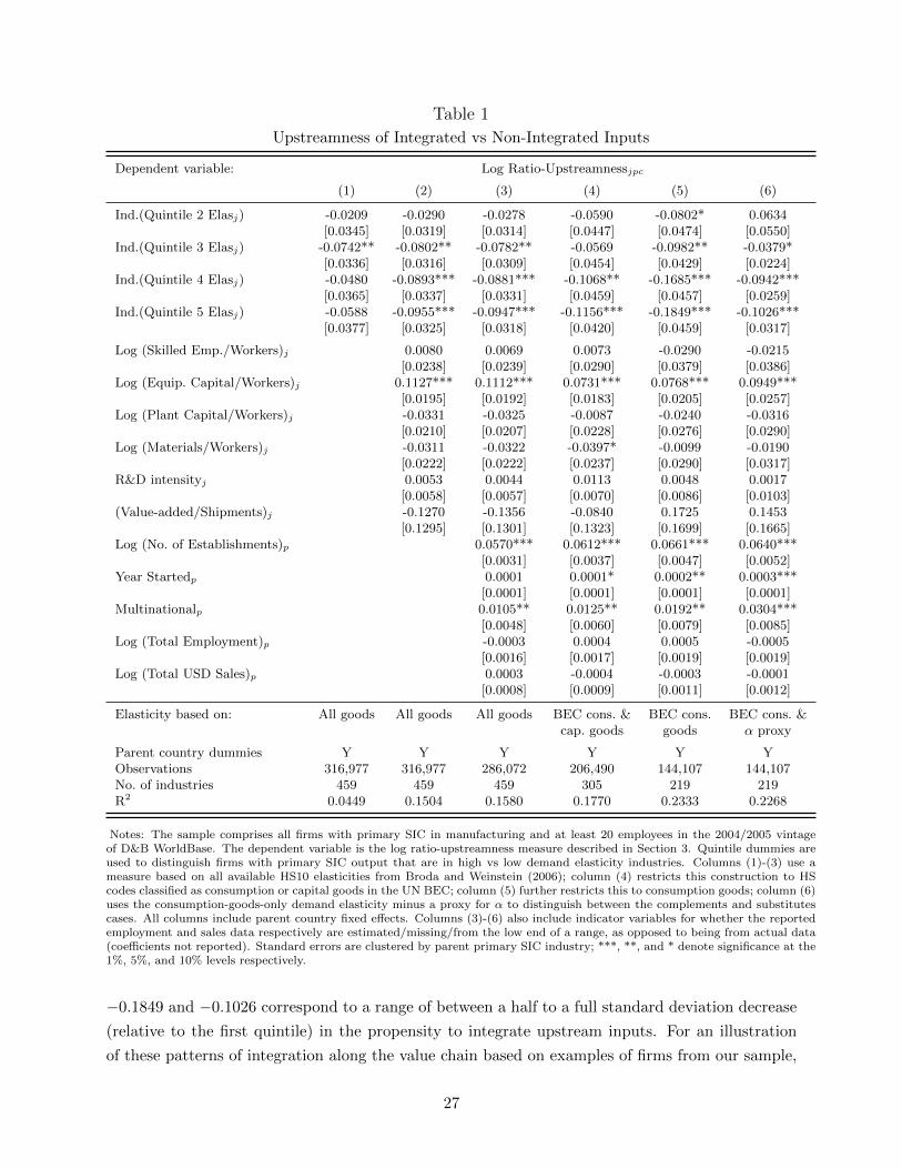
Table 1

Upstreamness of Integrated vs Non-Integrated Inputs

Dependent variable: Log Ratio-Upstreamnessjpc

(1) (2) (3) (4) (5) (6)

Ind.(Quintile 2 Elasj) -0.0209 -0.0290 -0.0278 -0.0590 -0.0802* 0.0634[0.0345] [0.0319] [0.0314] [0.0447] [0.0474] [0.0550]

Ind.(Quintile 3 Elasj) -0.0742** -0.0802** -0.0782** -0.0569 -0.0982** -0.0379*[0.0336] [0.0316] [0.0309] [0.0454] [0.0429] [0.0224]

Ind.(Quintile 4 Elasj) -0.0480 -0.0893*** -0.0881*** -0.1068** -0.1685*** -0.0942***[0.0365] [0.0337] [0.0331] [0.0459] [0.0457] [0.0259]

Ind.(Quintile 5 Elasj) -0.0588 -0.0955*** -0.0947*** -0.1156*** -0.1849*** -0.1026***[0.0377] [0.0325] [0.0318] [0.0420] [0.0459] [0.0317]

Log (Skilled Emp./Workers)j 0.0080 0.0069 0.0073 -0.0290 -0.0215[0.0238] [0.0239] [0.0290] [0.0379] [0.0386]

Log (Equip. Capital/Workers)j 0.1127*** 0.1112*** 0.0731*** 0.0768*** 0.0949***[0.0195] [0.0192] [0.0183] [0.0205] [0.0257]

Log (Plant Capital/Workers)j -0.0331 -0.0325 -0.0087 -0.0240 -0.0316[0.0210] [0.0207] [0.0228] [0.0276] [0.0290]

Log (Materials/Workers)j -0.0311 -0.0322 -0.0397* -0.0099 -0.0190[0.0222] [0.0222] [0.0237] [0.0290] [0.0317]

R&D intensityj 0.0053 0.0044 0.0113 0.0048 0.0017[0.0058] [0.0057] [0.0070] [0.0086] [0.0103]

(Value-added/Shipments)j -0.1270 -0.1356 -0.0840 0.1725 0.1453[0.1295] [0.1301] [0.1323] [0.1699] [0.1665]

Log (No. of Establishments)p 0.0570*** 0.0612*** 0.0661*** 0.0640***[0.0031] [0.0037] [0.0047] [0.0052]

Year Startedp 0.0001 0.0001* 0.0002** 0.0003***[0.0001] [0.0001] [0.0001] [0.0001]

Multinationalp 0.0105** 0.0125** 0.0192** 0.0304***[0.0048] [0.0060] [0.0079] [0.0085]

Log (Total Employment)p -0.0003 0.0004 0.0005 -0.0005[0.0016] [0.0017] [0.0019] [0.0019]

Log (Total USD Sales)p 0.0003 -0.0004 -0.0003 -0.0001[0.0008] [0.0009] [0.0011] [0.0012]

Elasticity based on: All goods All goods All goods BEC cons. & BEC cons. BEC cons. &cap. goods goods α proxy

Parent country dummies Y Y Y Y Y YObservations 316,977 316,977 286,072 206,490 144,107 144,107No. of industries 459 459 459 305 219 219R2 0.0449 0.1504 0.1580 0.1770 0.2333 0.2268

Notes: The sample comprises all firms with primary SIC in manufacturing and at least 20 employees in the 2004/2005 vintageof D&B WorldBase. The dependent variable is the log ratio-upstreamness measure described in Section 3. Quintile dummies areused to distinguish firms with primary SIC output that are in high vs low demand elasticity industries. Columns (1)-(3) use ameasure based on all available HS10 elasticities from Broda and Weinstein (2006); column (4) restricts this construction to HScodes classified as consumption or capital goods in the UN BEC; column (5) further restricts this to consumption goods; column (6)uses the consumption-goods-only demand elasticity minus a proxy for α to distinguish between the complements and substitutescases. All columns include parent country fixed effects. Columns (3)-(6) also include indicator variables for whether the reportedemployment and sales data respectively are estimated/missing/from the low end of a range, as opposed to being from actual data(coefficients not reported). Standard errors are clustered by parent primary SIC industry; ***, **, and * denote significance at the1%, 5%, and 10% levels respectively.

−0.1849 and −0.1026 correspond to a range of between a half to a full standard deviation decrease

(relative to the first quintile) in the propensity to integrate upstream inputs. For an illustration

of these patterns of integration along the value chain based on examples of firms from our sample,

27

please see Figures A-2 and A-3 in Section A-3 of the Online Appendix.

We turn next to assess the validity of prediction P.2 (Cross). For this, we augment the specifi-

cations in (17) in order to uncover the effects of upstream contractibility on integration:

log Ratio-Upstreamnessjpc = β0 +5∑

n=1

βUn1(ρj ∈ Quintn(ρ))× Upstream-Contractibilityj

+5∑

n=2

βn1(ρj ∈ Quintn(ρ)) + βXXj + βWWp +Dc + εjpc. (18)

Relative to (17), we now further interact each of the quintile dummies with Upstream-Contractibilityj ;

based on prediction P.2 (Cross), we would expect βU1 < 0 and βU5 > 0 in this regression.

The results from estimating (18) are reported in Table 2. The main effects of the quintile

elasticity dummies exhibit a pattern similar to that in the more parsimonious regressions in Table

1, with negative and significant coefficients especially as we transition to the higher quintiles.32

Of note, we find that in the complements case, a higher degree of upstream contractibility does

counteract the above tendency to outsource upstream inputs, as the coefficient on the fifth elasticity

quintile interacted with Upstream-Contractibilityj is positive and statistically significant (at the 1%

level) across all columns. Conversely, the interaction between the first elasticity quintile dummy and

Upstream-Contractibilityj bears the opposite sign, indicating that upstream contractibility instead

acts to raise the propensity to integrate downstream inputs in this latter case. This last pattern

appears most strongly in columns (1)-(3), where a demand elasticity associated with the output

industry ρj is used to separate the complements from the substitutes cases. In column (4), where

ρj−αj is used instead, the largest negative effect appears to be concentrated in the second elasticity

quintile. The overall message we obtain is nevertheless in line with prediction P.2 (Cross), which

relates integration decisions to the sequencing of high- versus low-contractibility inputs.

As discussed earlier, a key feature of the data is that integration is sparse. Proposition 4 shows

that this does not affect the qualitative predictions of our model, if we limit attention to the subset

of inputs over which integration is feasible. This suggests that a sharper test of our theory would

seek to drop inputs for which integration is prohibitively costly. In Table A-7 in Section A-3 of

the Online Appendix, we implement one such test by constructing the ratio-upstreamness measure

on the set of “ever-integrated” inputs only (as previously defined in Section 3), and re-running

the specifications from Table 2. Once again, the patterns line up with our model’s predictions:

regardless of the elasticity proxy used, the propensity to integrate upstream stages is lower for

firms in higher elasticity quintiles, but this effect is moderated in industries where production

features a greater degree of Upstream-Contractibilityj .

32We perform a test for whether the effect of being in the fifth quintile, evaluated at the median in-sample valueof Upstream-Contractibilityj in that fifth demand elasticity quintile, is in fact significantly different from zero. Thep-values reported in each column confirm that this is indeed the case, so that the propensity to integrate upstreaminputs is lower in the fifth relative to the first elasticity quintile; this holds true regardless of the variant of the elasticityproxy used across the columns. The role of upstream contractibility is also confirmed when using a median cutoffspecification to distinguish between the complements and substitutes cases (see Table A-6 in the Online Appendix).

28

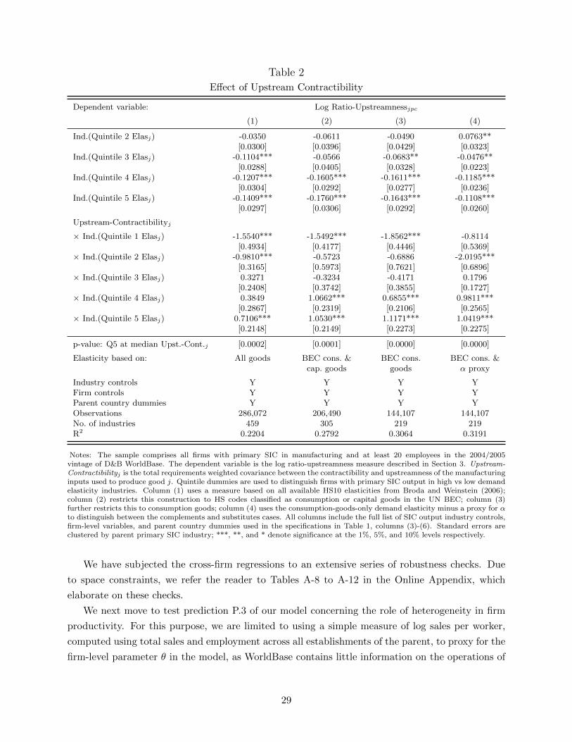
Table 2

Effect of Upstream Contractibility

Dependent variable: Log Ratio-Upstreamnessjpc

(1) (2) (3) (4)

Ind.(Quintile 2 Elasj) -0.0350 -0.0611 -0.0490 0.0763**[0.0300] [0.0396] [0.0429] [0.0323]

Ind.(Quintile 3 Elasj) -0.1104*** -0.0566 -0.0683** -0.0476**[0.0288] [0.0405] [0.0328] [0.0223]

Ind.(Quintile 4 Elasj) -0.1207*** -0.1605*** -0.1611*** -0.1185***[0.0304] [0.0292] [0.0277] [0.0236]

Ind.(Quintile 5 Elasj) -0.1409*** -0.1760*** -0.1643*** -0.1108***[0.0297] [0.0306] [0.0292] [0.0260]

Upstream-Contractibilityj

× Ind.(Quintile 1 Elasj) -1.5540*** -1.5492*** -1.8562*** -0.8114[0.4934] [0.4177] [0.4446] [0.5369]

× Ind.(Quintile 2 Elasj) -0.9810*** -0.5723 -0.6886 -2.0195***[0.3165] [0.5973] [0.7621] [0.6896]

× Ind.(Quintile 3 Elasj) 0.3271 -0.3234 -0.4171 0.1796[0.2408] [0.3742] [0.3855] [0.1727]

× Ind.(Quintile 4 Elasj) 0.3849 1.0662*** 0.6855*** 0.9811***[0.2867] [0.2319] [0.2106] [0.2565]

× Ind.(Quintile 5 Elasj) 0.7106*** 1.0530*** 1.1171*** 1.0419***[0.2148] [0.2149] [0.2273] [0.2275]

p-value: Q5 at median Upst.-Cont.j [0.0002] [0.0001] [0.0000] [0.0000]

Elasticity based on: All goods BEC cons. & BEC cons. BEC cons. &cap. goods goods α proxy

Industry controls Y Y Y YFirm controls Y Y Y YParent country dummies Y Y Y YObservations 286,072 206,490 144,107 144,107No. of industries 459 305 219 219R2 0.2204 0.2792 0.3064 0.3191

Notes: The sample comprises all firms with primary SIC in manufacturing and at least 20 employees in the 2004/2005vintage of D&B WorldBase. The dependent variable is the log ratio-upstreamness measure described in Section 3. Upstream-Contractibilityj is the total requirements weighted covariance between the contractibility and upstreamness of the manufacturinginputs used to produce good j. Quintile dummies are used to distinguish firms with primary SIC output in high vs low demandelasticity industries. Column (1) uses a measure based on all available HS10 elasticities from Broda and Weinstein (2006);column (2) restricts this construction to HS codes classified as consumption or capital goods in the UN BEC; column (3)further restricts this to consumption goods; column (4) uses the consumption-goods-only demand elasticity minus a proxy for αto distinguish between the complements and substitutes cases. All columns include the full list of SIC output industry controls,firm-level variables, and parent country dummies used in the specifications in Table 1, columns (3)-(6). Standard errors areclustered by parent primary SIC industry; ***, **, and * denote significance at the 1%, 5%, and 10% levels respectively.

We have subjected the cross-firm regressions to an extensive series of robustness checks. Due

to space constraints, we refer the reader to Tables A-8 to A-12 in the Online Appendix, which

elaborate on these checks.

We next move to test prediction P.3 of our model concerning the role of heterogeneity in firm

productivity. For this purpose, we are limited to using a simple measure of log sales per worker,

computed using total sales and employment across all establishments of the parent, to proxy for the

firm-level parameter θ in the model, as WorldBase contains little information on the operations of

29

firms beyond this.33 Moreover, when available, these variables are often based on estimates rather

than administrative data. To reduce the possible influence of such measurement error, we use a

dummy variable, 1(θp > θj,med), which identifies highly productive firms as those with log sales per

worker above the median value within each output industry j.

According to the first part of prediction P.3, more productive firms should integrate more inputs,

in both the complements and substitutes cases. To verify this, we estimate the following:

log (No. of Integrated Inputs)jpc = β0 +

5∑n=2

βn1(θp > θj,med)× 1(ρj ∈ Quintn(ρ))

+βWWp +Djc + εjpc. (19)

Note that the appropriate source of variation that we focus on here is that across firms within a

given industry, so the above regression is estimated with country-industry fixed effects, Djc.34

The results from running (19) are reported in the first two columns of Table 3. We use a

measure of ρj constructed using consumption-goods only demand elasticities in column (1), before

using the alternative proxy for ρj − αj in column (2). The estimated coefficients of the 1(θp >

θj,med) × 1(ρj ∈ Quintn(ρ)) interaction terms are almost all positive and significant, confirming

that more productive firms tend to integrate more SIC activities; this is regardless of whether the

industry in question falls closer to being in the substitutes or complements case.

According to the second part of prediction P.3, more productive firms should exhibit a higher

ratio-upstreamness in the complements case. The underlying intuition is that more productive

firms would be able to bear the higher fixed costs of integrating a larger set of stages within firm

boundaries, and so would engage in integrating some upstream inputs when compared against

smaller, less productive firms in the same industry. Conversely, the opposite would hold in the

substitutes case, with more productive firms instead featuring a lower ratio-upstreamness. To test

for such a pattern in the data, we therefore replace the dependent variable in (19) with log Ratio-

Upstreamnessjpc and re-estimate the regression. The results are reported in columns (3)-(4) of

Table 3, these being based respectively on the ρj and ρj −αj proxies used in the first two columns

of the same table. The patterns that emerge are entirely in line with prediction P.3: the estimated

coefficient of the interaction term between 1(θp > θj,med) and the first quintile of ρj is negative and

significant, while the corresponding coefficient for the fifth quintile of ρj is positive and significant.

We obtain a very similar set of estimates in columns (5)-(6), where we use the version of the ratio-

upstreamness measure that is based on ever-integrated inputs. Thus, more productive firms have

a lower (respectively, higher) relative propensity to integrate upstream inputs when the elasticity

of demand for their final product is low (respectively, high).35

33Because log sales per worker is a measure of revenue-based productivity, it captures variation in both θ and A.Proposition 3 shows, however, that our comparative statics results hold regardless of whether one varies θ or A.

34We can thus include the firm-level variables, Wp, in (19), but not the vector of industry controls, Xj .35The alert reader may wonder why we do not explore triple interactions between the demand elasticity quintiles,

the high-productivity dummy, and the upstream contractibility variable. However, as discussed in the proof ofProposition 3 in Section A-1 of the Online Appendix, it is in general not possible to sign this effect in the theory.

30

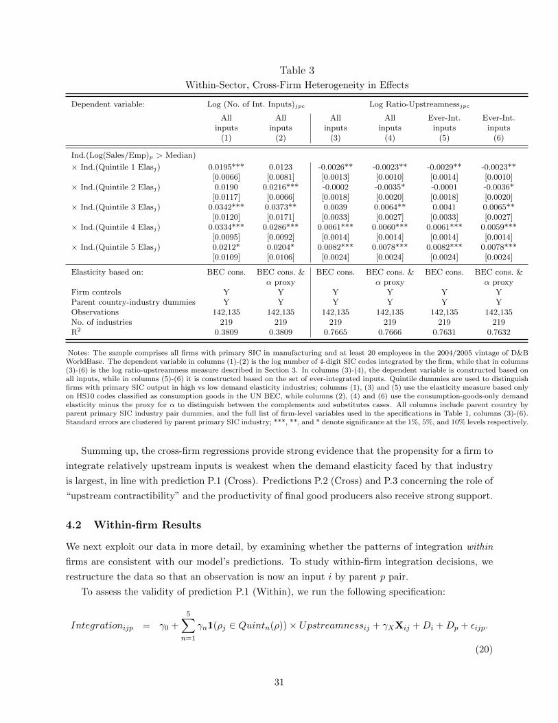
Table 3

Within-Sector, Cross-Firm Heterogeneity in Effects

Dependent variable: Log (No. of Int. Inputs)jpc Log Ratio-Upstreamnessjpc

All All All All Ever-Int. Ever-Int.inputs inputs inputs inputs inputs inputs

(1) (2) (3) (4) (5) (6)

Ind.(Log(Sales/Emp)p > Median)

× Ind.(Quintile 1 Elasj) 0.0195*** 0.0123 -0.0026** -0.0023** -0.0029** -0.0023**[0.0066] [0.0081] [0.0013] [0.0010] [0.0014] [0.0010]

× Ind.(Quintile 2 Elasj) 0.0190 0.0216*** -0.0002 -0.0035* -0.0001 -0.0036*[0.0117] [0.0066] [0.0018] [0.0020] [0.0018] [0.0020]

× Ind.(Quintile 3 Elasj) 0.0342*** 0.0373** 0.0039 0.0064** 0.0041 0.0065**[0.0120] [0.0171] [0.0033] [0.0027] [0.0033] [0.0027]

× Ind.(Quintile 4 Elasj) 0.0334*** 0.0286*** 0.0061*** 0.0060*** 0.0061*** 0.0059***[0.0095] [0.0092] [0.0014] [0.0014] [0.0014] [0.0014]

× Ind.(Quintile 5 Elasj) 0.0212* 0.0204* 0.0082*** 0.0078*** 0.0082*** 0.0078***[0.0109] [0.0106] [0.0024] [0.0024] [0.0024] [0.0024]

Elasticity based on: BEC cons. BEC cons. & BEC cons. BEC cons. & BEC cons. BEC cons. &α proxy α proxy α proxy

Firm controls Y Y Y Y Y YParent country-industry dummies Y Y Y Y Y YObservations 142,135 142,135 142,135 142,135 142,135 142,135No. of industries 219 219 219 219 219 219R2 0.3809 0.3809 0.7665 0.7666 0.7631 0.7632

Notes: The sample comprises all firms with primary SIC in manufacturing and at least 20 employees in the 2004/2005 vintage of D&BWorldBase. The dependent variable in columns (1)-(2) is the log number of 4-digit SIC codes integrated by the firm, while that in columns(3)-(6) is the log ratio-upstreamness measure described in Section 3. In columns (3)-(4), the dependent variable is constructed based onall inputs, while in columns (5)-(6) it is constructed based on the set of ever-integrated inputs. Quintile dummies are used to distinguishfirms with primary SIC output in high vs low demand elasticity industries; columns (1), (3) and (5) use the elasticity measure based onlyon HS10 codes classified as consumption goods in the UN BEC, while columns (2), (4) and (6) use the consumption-goods-only demandelasticity minus the proxy for α to distinguish between the complements and substitutes cases. All columns include parent country byparent primary SIC industry pair dummies, and the full list of firm-level variables used in the specifications in Table 1, columns (3)-(6).Standard errors are clustered by parent primary SIC industry; ***, **, and * denote significance at the 1%, 5%, and 10% levels respectively.

Summing up, the cross-firm regressions provide strong evidence that the propensity for a firm to

integrate relatively upstream inputs is weakest when the demand elasticity faced by that industry

is largest, in line with prediction P.1 (Cross). Predictions P.2 (Cross) and P.3 concerning the role of

“upstream contractibility” and the productivity of final good producers also receive strong support.

4.2 Within-firm Results

We next exploit our data in more detail, by examining whether the patterns of integration within

firms are consistent with our model’s predictions. To study within-firm integration decisions, we

restructure the data so that an observation is now an input i by parent p pair.

To assess the validity of prediction P.1 (Within), we run the following specification:

Integrationijp = γ0 +

5∑n=1

γn1(ρj ∈ Quintn(ρ))× Upstreamnessij + γXXij +Di +Dp + εijp.

(20)

31

The dependent variable is a 0-1 indicator for whether the firm p with primary output j has inte-

grated the input i within firm boundaries. The key explanatory variables are the terms involving

Upstreamnessij and its interactions with the different quintiles of the elasticity variable. We include

a full set of parent fixed effects, Dp, thus focusing on within-firm variation in Integrationijp; these

fixed effects also absorb any systematic differences arising from the identity of the output industry

or country of incorporation of the parent firm. When examining within-firm integration patterns

in this manner, our theory would suggest that γ1 > 0 and γ5 < 0.

We estimate (20) as a linear probability model, with standard errors clustered by i-j pair.

To avoid including firms for whom occurrences of integration are exceedingly rare, we restrict

the sample to parent firms that have integrated at least one manufacturing input other than the

parent’s output industry code. To keep the regressions tractable, we limit the sample to the top

100 manufacturing inputs i used by each industry j as ranked by the total requirements coefficient,

trij .36 Among the top-100 inputs, we further retain only those inputs i that are ever-integrated

by a parent firm in output j (as defined previously in Section A-7). This is done bearing in mind

the extension on sparse integration from Section 2.2.C: Including in the regression inputs for which

integration is not feasible could obscure our ability to test Proposition 4 cleanly, particularly in

this within-firm, cross-input specification.37

The regression in (20) includes a vector Xij , to capture other industry pair characteristics that

might be correlated with the propensity of a parent firm in industry j to integrate input i. It

includes three sets of variables. First, we control for the dummy variable Self-SICij , which is equal

to 1 if and only if i = j. The dependent variable in (20) always takes on a value of 1 when i = j, as

j ∈ I(j) by definition. Including this dummy thus allows us to focus on the effects of Upstreamnessij

for manufacturing inputs other than j.38 Second, we control for the overall importance of input i

in the production of j, as reflected in the log of the total requirements coefficient, trij .

Third, we include a series of variables to capture the proximity between two industries i

and j, which have been explored elsewhere in the empirical literature on the determinants of

firm ownership.39 Using the 1992 U.S. I-O Tables, we have constructed a measure of Upstream-

Complementarityij for each pair of industries, as the correlation between the direct requirements

coefficients of inputs k 6= i, j used in the production of i and j respectively. Similarly, we have con-

structed Downstream-Complementarityij as the correlation in the direct use of i and j (expressed

as a share of gross output in i and j respectively) across buying industries k 6= i, j. As argued by

Fan and Lang (2000), these measures capture the extent to which two industries enjoy economies

of scale in jointly procuring inputs, or in sharing marketing and distribution costs.40 We have

also constructed several measures of the relatedness of industries based on their factor intensities,

36The top 100 manufacturing inputs cover between 88-98% of the total requirements value of each output industry.37We report broadly similar results in Tables A-16 and A-17 in the Online Appendix when using all top-100 inputs.38The findings are very similar if we drop the self-SIC inputs entirely from the sample (see Tables A-16 and A-17

in the Online Appendix).39We are grateful to an anonymous referee for suggesting the inclusion of such variables.40While Fan and Lang (2000) take the average of these two complementarity measures in their study, we use each

of them as separate variables in our regressions.

32

as the absolute difference between industries i and j in their skill, equipment capital, plant cap-

ital, and R&D intensities respectively. As pointed out by Atalay et al. (2014), empirical studies

testing the resource-based view of the firm show that when firms expand, they enter industries

for which the resource (e.g., capital, skill, or R&D) requirements match the requirements of the

industries in which the firm had already been producing (see Montgomery and Hariharan, 1991;

Neffke and Henning, 2013). Last but not least, the dummy variables Same-SIC2ij and Same-SIC3ij

respectively identify industries that share the first two and the first three digits in their SIC codes.

Similar indicators have been widely used in the literature to capture the proximity between two

industries (e.g., Alfaro and Charlton, 2009). (Summary statistics for these industry-pair variables

are reported in Table A-4 in the Online Appendix.)

Rounding off the description of (20), in our most stringent specifications, we will introduce a

full set of input dummies, Di, to control for characteristics of each input that might affect a firm’s

propensity to integrate it. When these input fixed effects are used, only covariates that vary at the

input-output (i-j) pair level can be identified in the estimation.

Table 4 reports the results of the estimation of (20). Column (1) reports a parsimonious spec-

ification, in which we include the interactions between Upstreamnessij and the demand elasticity

dummies (constructed from consumption-goods elasticities only), the Self-SICij dummy, and log

trij . The negative coefficients obtained on Upstreamnessij point to a lower propensity to integrate

upstream inputs across all output industries in general. However, in line with the weaker statement

in prediction P.1 (Within), firms are significantly less likely to integrate upstream inputs in the

complements case compared to the substitutes case: the γ1 coefficient for the first elasticity quintile

interaction is significantly larger than the γ5 coefficient for the fifth-quintile interaction. The test

for the equality of these coefficients is rejected (see the p-values near the bottom of the table).

In the columns that follow, we include the different measures of proximity between industries i

and j. Controlling for Upstream-Complementarityij and Downstream-Complementarityij in column

(2), we now find that firms in the lowest demand elasticity quintile are more likely to integrate

upstream inputs (γ1 > 0 and significant at the 10% level), while those in the highest elasticity

quintile are more likely to integrate downstream inputs (γ5 < 0 and significant at the 1% level).

Thus, including proxies of the scope for cost savings in input procurement and in marketing and

distribution leads us to find support for the stronger version of our model’s predictions.41 This

pattern persists when we add the measures of factor intensity differences (column (3)), the dummies

for sharing the same first two or first three SIC digits (column (4)), as well as input fixed effects

(column (5)). When instead we use the ρj −αj proxy to distinguish between the complements and

substitutes cases (column (6)), we lose the positive sign on the γ1 coefficient, but the propensity to

41The correlation between Upstreamnessij and Upstream-Complementarityij is −0.413, while that withDownstream-Complementarityij is −0.406; these are computed over the restricted subset of ever-integrated top-100 manufacturing inputs, but the correlations are similar if all top-100 manufacturing inputs are included. There isthus a tendency for inputs that exhibit weaker complementarities in either procurement or marketing/distribution tobe located more upstream relative to the final-good industry. This accounts for why the Upstreamnessij interactioncoefficients either move into less negative or more positive terrain once the effects of upstream- and downstream-complementarities are directly controlled for in column (2), Table 4.

33

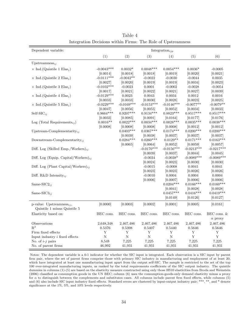
Table 4

Integration Decisions within Firms: The Role of Upstreamness

Dependent variable: Integrationijp

(1) (2) (3) (4) (5) (6)

Upstreamnessij

× Ind.(Quintile 1 Elasj) -0.0043*** 0.0032* 0.0048*** 0.0054*** 0.0036* -0.0005[0.0014] [0.0018] [0.0018] [0.0019] [0.0020] [0.0021]

× Ind.(Quintile 2 Elasj) -0.0111*** -0.0042** -0.0022 -0.0030 -0.0044 0.0035[0.0027] [0.0020] [0.0019] [0.0019] [0.0034] [0.0023]

× Ind.(Quintile 3 Elasj) -0.0102*** -0.0023 0.0001 -0.0002 -0.0028 -0.0054[0.0017] [0.0021] [0.0022] [0.0021] [0.0027] [0.0039]

× Ind.(Quintile 4 Elasj) -0.0129*** 0.0023 0.0043 0.0034 0.0012 0.0016[0.0033] [0.0033] [0.0030] [0.0028] [0.0023] [0.0025]

× Ind.(Quintile 5 Elasj) -0.0229*** -0.0169*** -0.0153*** -0.0146*** -0.0077** -0.0079**[0.0047] [0.0056] [0.0055] [0.0052] [0.0034] [0.0033]

Self-SICij 0.9664*** 0.9207*** 0.9134*** 0.8823*** 0.8517*** 0.8517***[0.0033] [0.0085] [0.0091] [0.0164] [0.0177] [0.0176]

Log (Total Requirementsij) 0.0016** 0.0022*** 0.0034*** 0.0028*** 0.0035*** 0.0038***[0.0008] [0.0008] [0.0008] [0.0008] [0.0012] [0.0012]

Upstream-Complementarityij 0.0403*** 0.0367*** 0.0174*** 0.0200*** 0.0200***[0.0039] [0.0038] [0.0037] [0.0037] [0.0037]

Downstream-Complementarityij 0.0284*** 0.0260*** 0.0129** 0.0171*** 0.0163***[0.0065] [0.0064] [0.0052] [0.0059] [0.0057]

Diff. Log (Skilled Emp./Workers)ij -0.0170*** -0.0156*** -0.0213*** -0.0217***[0.0039] [0.0037] [0.0044] [0.0045]

Diff. Log (Equip. Capital/Workers)ij -0.0034 -0.0038* -0.0089*** -0.0089***[0.0024] [0.0023] [0.0030] [0.0030]

Diff. Log (Plant Capital/Workers)ij -0.0015 -0.0008 0.0041 0.0041[0.0023] [0.0023] [0.0026] [0.0026]

Diff. R&D Intensityij -0.0010 0.0004 0.0004 0.0004[0.0006] [0.0007] [0.0006] [0.0006]

Same-SIC2ij 0.0204*** 0.0166*** 0.0160***[0.0041] [0.0028] [0.0028]

Same-SIC3ij 0.0457*** 0.0416*** 0.0419***[0.0149] [0.0126] [0.0127]

p-value: Upstreamnessij , [0.0000] [0.0003] [0.0002] [0.0001] [0.0005] [0.0161]Quintile 1 minus Quintile 5

Elasticity based on: BEC cons. BEC cons. BEC cons. BEC cons. BEC cons. BEC cons. &α proxy

Observations 2,648,348 2,467,486 2,467,486 2,467,486 2,467,486 2,467,486R2 0.5376 0.5398 0.5407 0.5440 0.5646 0.5646Firm fixed effects Y Y Y Y Y YInput industry i fixed effects N N N N Y YNo. of i-j pairs 8,548 7,225 7,225 7,225 7,225 7,225No. of parent firms 46,992 41,931 41,931 41,931 41,931 41,931

Notes: The dependent variable is a 0-1 indicator for whether the SIC input is integrated. Each observation is a SIC input by parentfirm pair, where the set of parent firms comprise those with primary SIC industry in manufacturing and employment of at least 20,which have integrated at least one manufacturing input apart from the output self-SIC. The sample is restricted to the set of the top100 ever-integrated manufacturing inputs, as ranked by the total requirements coefficients of the SIC output industry. The quintiledummies in columns (1)-(5) are based on the elasticity measure constructed using only those HS10 elasticities from Broda and Weinstein(2006) classified as consumption goods in the UN BEC; column (6) uses the consumption-goods-only demand elasticity minus a proxyfor α to distinguish between the complements and substitutes cases. All columns include parent firm fixed effects, while columns (5)and (6) also include SIC input industry fixed effects. Standard errors are clustered by input-output industry pair; ***, **, and * denotesignificance at the 1%, 5%, and 10% levels respectively.

34

integrate upstream remains significantly weaker in the fifth relative to the first elasticity quintile.

It is worth noting that the estimated coefficients for the variables capturing the proximity

between two industries are broadly consistent with theories that emphasize the importance of

intangibles in firm boundary choices (Atalay et al., 2014). In particular, one interpretation of the

positive and significant effects of the upstream- and downstream-complementarity measures is that

firms are more likely to engage in integration when it is easier to share intangible knowledge related

to common input procurement or marketing and distribution practices. Likewise, the regressions

indicate that firms are more likely to integrate inputs with similar skill-intensity requirements as the

parent’s output industry, possibly because similarity of skills is important for facilitating the transfer

of intangible assets from parents to subsidiaries. It is thus reassuring that despite controlling (albeit

imperfectly) for these additional motives behind firm boundary choices, we continue to find evidence

supporting the subtle predictions of our model on how upstreamness affects integration patterns.

As a final exercise, we empirically assess prediction P.2 (Within). For this, we include inter-

actions between the elasticity quintiles ρj and Contractibility-up-to-iij , where the latter variable

captures the contractibility of all inputs up to i in the production of j:

Integrationijp = γ0 +

5∑n=1

γn1(ρj ∈ Quintn(ρ))× Contractibility-up-to-iij

+γXXij +Di +Dp + εijp. (21)

Recall that Contractibility-up-to-iij was constructed in (16) as an empirical proxy for∫ i0 (ψ(k))

α1−α dk∫ 1

0 (ψ(k))α

1−α dk

from the model. Looking back at the expression for the optimal bargaining share, β∗(m), in

equation (10), one would then expect that Contractibility-up-to-iij would raise the propensity to

integrate input i if industry j came under the complements case, while having the opposite effect

in the substitutes case. This would lead us to expect that γ1 < 0 and γ5 > 0, although finding that

γ5 > γ1 > 0 would be consistent with the weaker statement in prediction P.2 (Within).

The results from estimating (21) are reported in Table 5. As in Table 4, we begin by reporting

a parsimonious specification in which we only include the interactions between Contractibility-up-

to-iij and the demand elasticity quintiles, the self-SIC dummy, and log trij (column (1)). While

the interactions with Contractibility-up-to-iij all yield positive coefficients, the magnitude of these

coefficients is largest in the highest elasticity quintile. (The difference between the first and fifth

quintile coefficients is statistically significant; see the p-value at the bottom of the table.) The

results obtained are similar when controlling for the additional industry-pair variables related to

the proximity of industries (columns (2)-(4)), controlling for input industry fixed effects (column

(5)), as well as when using the proxy of αj to refine the demand elasticity quintiles (column (6)).

Consistent with prediction P.2 (Within) of our model, the findings of Table 5 thus show that a

greater contractibility of inputs upstream of i increases the propensity to integrate input i more

for firms facing a higher elasticity of demand for their final product.

We have performed a series of additional estimations to verify the robustness of the within-firm

35

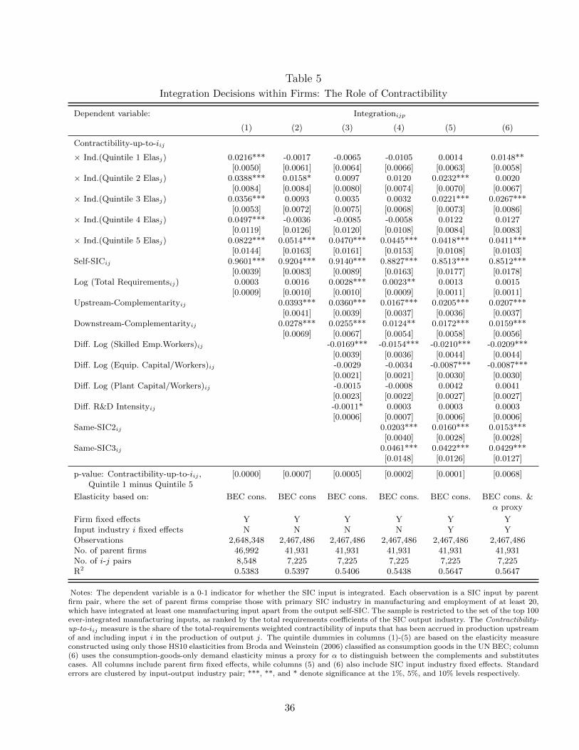
Table 5

Integration Decisions within Firms: The Role of Contractibility

Dependent variable: Integrationijp

(1) (2) (3) (4) (5) (6)

Contractibility-up-to-iij

× Ind.(Quintile 1 Elasj) 0.0216*** -0.0017 -0.0065 -0.0105 0.0014 0.0148**[0.0050] [0.0061] [0.0064] [0.0066] [0.0063] [0.0058]

× Ind.(Quintile 2 Elasj) 0.0388*** 0.0158* 0.0097 0.0120 0.0232*** 0.0020[0.0084] [0.0084] [0.0080] [0.0074] [0.0070] [0.0067]

× Ind.(Quintile 3 Elasj) 0.0356*** 0.0093 0.0035 0.0032 0.0221*** 0.0267***[0.0053] [0.0072] [0.0075] [0.0068] [0.0073] [0.0086]

× Ind.(Quintile 4 Elasj) 0.0497*** -0.0036 -0.0085 -0.0058 0.0122 0.0127[0.0119] [0.0126] [0.0120] [0.0108] [0.0084] [0.0083]

× Ind.(Quintile 5 Elasj) 0.0822*** 0.0514*** 0.0470*** 0.0445*** 0.0418*** 0.0411***[0.0144] [0.0163] [0.0161] [0.0153] [0.0108] [0.0103]

Self-SICij 0.9601*** 0.9204*** 0.9140*** 0.8827*** 0.8513*** 0.8512***[0.0039] [0.0083] [0.0089] [0.0163] [0.0177] [0.0178]

Log (Total Requirementsij) 0.0003 0.0016 0.0028*** 0.0023** 0.0013 0.0015[0.0009] [0.0010] [0.0010] [0.0009] [0.0011] [0.0011]

Upstream-Complementarityij 0.0393*** 0.0360*** 0.0167*** 0.0205*** 0.0207***[0.0041] [0.0039] [0.0037] [0.0036] [0.0037]

Downstream-Complementarityij 0.0278*** 0.0255*** 0.0124** 0.0172*** 0.0159***[0.0069] [0.0067] [0.0054] [0.0058] [0.0056]

Diff. Log (Skilled Emp.Workers)ij -0.0169*** -0.0154*** -0.0210*** -0.0209***[0.0039] [0.0036] [0.0044] [0.0044]

Diff. Log (Equip. Capital/Workers)ij -0.0029 -0.0034 -0.0087*** -0.0087***[0.0021] [0.0021] [0.0030] [0.0030]

Diff. Log (Plant Capital/Workers)ij -0.0015 -0.0008 0.0042 0.0041[0.0023] [0.0022] [0.0027] [0.0027]

Diff. R&D Intensityij -0.0011* 0.0003 0.0003 0.0003[0.0006] [0.0007] [0.0006] [0.0006]

Same-SIC2ij 0.0203*** 0.0160*** 0.0153***[0.0040] [0.0028] [0.0028]

Same-SIC3ij 0.0461*** 0.0422*** 0.0429***[0.0148] [0.0126] [0.0127]

p-value: Contractibility-up-to-iij , [0.0000] [0.0007] [0.0005] [0.0002] [0.0001] [0.0068]Quintile 1 minus Quintile 5

Elasticity based on: BEC cons. BEC cons BEC cons. BEC cons. BEC cons. BEC cons. &α proxy

Firm fixed effects Y Y Y Y Y YInput industry i fixed effects N N N N Y YObservations 2,648,348 2,467,486 2,467,486 2,467,486 2,467,486 2,467,486No. of parent firms 46,992 41,931 41,931 41,931 41,931 41,931No. of i-j pairs 8,548 7,225 7,225 7,225 7,225 7,225R2 0.5383 0.5397 0.5406 0.5438 0.5647 0.5647

Notes: The dependent variable is a 0-1 indicator for whether the SIC input is integrated. Each observation is a SIC input by parentfirm pair, where the set of parent firms comprise those with primary SIC industry in manufacturing and employment of at least 20,which have integrated at least one manufacturing input apart from the output self-SIC. The sample is restricted to the set of the top 100ever-integrated manufacturing inputs, as ranked by the total requirements coefficients of the SIC output industry. The Contractibility-up-to-iij measure is the share of the total-requirements weighted contractibility of inputs that has been accrued in production upstreamof and including input i in the production of output j. The quintile dummies in columns (1)-(5) are based on the elasticity measureconstructed using only those HS10 elasticities from Broda and Weinstein (2006) classified as consumption goods in the UN BEC; column(6) uses the consumption-goods-only demand elasticity minus a proxy for α to distinguish between the complements and substitutescases. All columns include parent firm fixed effects, while columns (5) and (6) also include SIC input industry fixed effects. Standarderrors are clustered by input-output industry pair; ***, **, and * denote significance at the 1%, 5%, and 10% levels respectively.

36

results (see Section A-3 of the Online Appendix). Tables A-14 and A-15 confirm the robustness of

our results concerning the role of upstreamness and contractibility in shaping integration decisions

along the value chain, when we restrict the sample to different subsets of firms (single-establishment

firms, domestic firms, and multinationals). Tables A-16 and A-17 show that our results are similar

if we: (i) drop parent firms that do not have an integrated input (apart from the self-SIC) among

the top-100 manufacturing inputs as ranked by total requirements value; (ii) focus on parents that

have integrated at least three of their top-100 manufacturing inputs; (iii) drop the self-SIC from

the estimation; and (iv) include all top-100 manufacturing inputs (instead of focusing on the subset

of ever-integrated inputs). In Table A-17, we show that the estimated effects of Contractibility-up-

to-iij are robust to controlling for a measure of the contractibility of input i itself.

5 Conclusion

In this paper, we show how detailed data on the activities of firms around the world can be

combined with information from standard Input-Output tables to study integration choices along

value chains. Building on Antras and Chor (2013), we first describe a property-rights model in

which a firm’s boundaries are shaped by characteristics of the different stages of production and

their position along the value chain. As available theoretical frameworks of sequential production

are highly stylized, a key contribution here is to develop a richer model of firm behavior that can

guide an empirical analysis using firm-level data.

To assess the evidence, we use the WorldBase dataset, which contains establishment-level in-

formation on the activities of firms located in a large set of countries. The richness of our data

allows us to run specifications that exploit variation in organizational features across firms, as well

as within firms and across their various manufacturing stages. In line with our model’s predictions,

we find that whether a firm integrates suppliers located upstream or downstream depends crucially

on the elasticity of demand faced by the firm. Moreover, the propensity to integrate upstream

(as opposed to downstream) inputs depends on the extent to which contractible inputs tend to be

located in the early or late stages of the value chain, as well as on the productivity of final good

producers. The patterns that we uncover provide strong evidence that considerations driven by

contractual frictions critically shape firms’ ownership decisions along their value chains.

Although we have interpreted our empirical findings as being supportive of the relevance of

a property-rights model of firm boundaries in a sequential production environment, they could

in principle be consistent with alternative theories. The key features of our model that generate

predictions in line with the patterns observed in the data are as follows: (i) relative to integration,

non-integration is associated with higher-powered incentives for suppliers; (ii) variation in the de-

mand elasticity affects the relative importance of eliciting high effort or investments in upstream

versus downstream stages; and (iii) higher contractibility is associated with less inefficient invest-

ments. As argued by Tadelis and Willamson (2013), one could envision transaction-cost models

of firm boundaries satisfying properties (i) and (iii), which coupled with our model of sequential

37

production would also produce feature (ii). In addition, when discussing our empirical results

(specifically, the within-firm regressions) we have highlighted some patterns that are consistent

with alternative theories (e.g., Atalay et al., 2014) advocating that common ownership allows firms

to efficiently move intangible inputs across their production units.

References

Acemoglu, Daron, Pol Antras, and Elhanan Helpman (2007), “Contracts and Technology Adoption,” Amer-ican Economic Review 97(3): 916-943.

Acemoglu, Daron, Simon Johnson, and Todd Mitton (2009), “Determinants of Vertical Integration: Finan-cial Development and Contracting Costs,” Journal of Finance 63(3): 1251-1290.

Alfaro, Laura, and Andrew Charlton (2009), “Intra-Industry Foreign Direct Investment,” American Eco-nomic Review 99(5): 2096-2119.

Alfaro, Laura, and Maggie Xiaoyang Chen (2014), “The Global Agglomeration of Multinational Firms,”Journal of International Economics 94(2): 263-276.

Alfaro, Laura, Paola Conconi, Harald Fadinger, and Andrew Newman (2016), “Do Price Determine VerticalIntegration?” Review of Economic Studies 83(3): 855-888.

Antras, Pol (2003), “Firms, Contracts, and Trade Structure,” Quarterly Journal of Economics 118(4):1375-1418.

Antras, Pol (2014), “Grossman-Hart (1986) Goes Global: Incomplete Contracts, Property Rights, and theInternational Organization of Production,” Journal of Law, Economics and Organization 30: 118-175.

Antras, Pol (2015), Global Production: Firms, Contracts and Trade Structure, Princeton University Press.

Antras, Pol, and Davin Chor (2013), “Organizing the Global Value Chain,” Econometrica 81(6): 2127-2204.

Antras, Pol, Davin Chor, Thibault Fally, and Russell Hillberry (2012), “Measuring the Upstreamness ofProduction and Trade Flows,” American Economic Review Papers & Proceedings 102(3): 412-416.

Antras, Pol, and Alonso de Gortari (2017), “On the Geography of Global Value Chains,” mimeo.

Antras, Pol, and Elhanan Helpman (2004), “Global Sourcing,” Journal of Political Economy 112(3): 552-580.

Atalay, Enghin, Ali Hortacsu, and Chad Syverson (2014), “Vertical Integration and Input Flows,”AmericanEconomic Review 104(4): 1120-1148.

Baker, George P. and Thomas N. Hubbard (2004), “Contractibility and Asset Ownership: On-Board Com-puters and Governance in U.S. Trucking,”Quarterly Journal of Economics 119 (4): 1443-1479.

Baldwin, Richard, and Anthony Venables (2013), “Spiders and Snakes: Offshoring and Agglomeration inthe Global Economy,” Journal of International Economics 90(2): 245-254.

Becker, Randy A., and Wayne B. Gray (2009), “NBER-CES Manufacturing Industry Database (1958-2005)”.

Bresnahan, Timothy, and Jonathan Levin (2012), “Vertical Integration and Market Structure,” in TheHandbook of Organizational Economics, Princeton University Press.

Broda, Christian, and David Weinstein (2006), “Globalization and the Gains from Variety,” QuarterlyJournal of Economics 121(2): 541-585.

Brown, Clair, and Greg Linden (2005), “Offshoring in the Semiconductor Industry: A Historical Perspec-tive,” Brookings Trade Forum (Offshoring White-Collar Work), pp.279-333.

38

Cameron, Colin, Jonah Gelbach, and Douglas Miller (2011), “Robust Inference with Multi-way Clustering,”Journal of Business and Economic Statistics 29(2): 238-249.

Costinot, Arnaud, Jonathan Vogel, and Su Wang (2013), “An Elementary Theory of Global Supply Chains,”Review of Economic Studies 80(1): 109-144.

Corcos, Gregory, Delphine Irac, Delphine M., Giordano Mion, and Thierry Verdier (2013), “The Determi-nants of Intrafirm Trade: Evidence from French Firms,” Review of Economics and Statistics 95(3):825-838.

Defever, Fabrice, and Farid Toubal (2013), “Productivity, Relationship-Specific Inputs and the SourcingModes of Multinationals,” Journal of Economic Behavior and Organization 94: 345-357.

Del Prete, Davide, and Armando Rungi (2017), “Organizing the Global Value Chain: A Firm Level Test,”Journal of International Economics 109: 16-30.

Dietzenbacher, Erik, Isidoro Romero Luna, and Niels S. Bosma (2005), “Using Average PropogrationLengths to Identify Production Chains in the Andalusian Economy,” Estudios de Economia Aplicada23(2): 405-422.

Dıez, Federico (2014), “The Asymmetric Effects of Tariffs on Intra-firm Trade and Offshoring Decisions,”Journal of International Economics 93(1): 76-91.

Dixit, Avinash, and Gene Grossman (1982), “Trade and Protection with Multistage Production,” Reviewof Economic Studies 49(4): 583-594.

Fajgelbaum, Pablo, Gene Grossman, and Elhanan Helpman (2015), “A Linder Hypothesis for ForeignDirect Investment,” Review of Economic Studies 82(1): 83-121.

Fally, Thibault (2012), “On the Fragmentation of Production in the U.S.,” mimeo.

Fally, Thibault, and Russell Hillbery (2014), “A Coasian Model of International Production Chains,” mimeo.

Fan, Joseph P. H., and Larry H. P. Lang (2000), “The Measurement of Relatedness: An Application toCorporate Diversification,” Journal of Business 73(4): 629-660.

Feenstra, Robert C., John Romalis, and Peter K. Schott, (2002), “U.S. Imports, Exports and Tariff Data,1989-2001,” NBER Working Paper 9387.

Grossman, Sanford J., and Hart, Oliver D. (1986), “The Costs and Benefits of Ownership: A Theory ofVertical and Lateral Integration,” Journal of Political Economy 94(4): 691-719.

Johnson, Robert C., and Guillermo Noguera (2012), “Accounting for Intermediates: Production Sharingand Trade in Value Added,” Journal of International Economics 86(2): 224-236.

Kikuchi, Tomoo, Kazuo Nishimura, and John Stachurski (2017), “Span of Control, Transaction Costs andthe Structure of Production Chains,” Theoretical Economics, forthcoming.

Lafontaine, Francine, and Margaret Slade (2007), “Vertical Integration and Firm Boundaries: The Evi-dence,” Journal of Economic Literature 45(3): 629-685.

Luck, Philip (2016), “Global Supply Chains, Firm Scope and Vertical Integration: Evidence from China,”Journal of Economic Geography, forthcoming.

Montgomery, Cynthia A., and S. Hariharan (1991), “Diversified Expansion by Large Established Firms,”Journal of Economic Behavior and Organization 15(1): 71-89.

Neffke, Frank, and Martin Henning (2013), “Skill Relatedness and Firm Diversification,”Strategic Manage-ment Journal 34: 297-316.

Nunn, Nathan (2007), “Relationship-Specificity, Incomplete Contracts and the Pattern of Trade,” QuarterlyJournal of Economics 122(2): 569-600.

Nunn, Nathan, and Daniel Trefler (2008), “The Boundaries of the Multinational Firm: An EmpiricalAnalysis,” in E. Helpman, D. Marin, and T. Verdier (eds.), The Organization of Firms in a GlobalEconomy, Harvard University Press.

39

Nunn, Nathan, and Daniel Trefler (2013), “Incomplete Contracts and the Boundaries of the MultinationalFirm,” Journal of Economic Behavior and Organization 94: 330-344.

Ramondo, Natalia, Veronica Rappoport, and Kim Ruhl (2016), “Horizontal versus Vertical Foreign DirectInvestment: Evidence from U.S. Multinationals,” Journal of International Economics, 98(1): 51-59.

Rauch, James E. (1999), “Networks versus Markets in International Trade,” Journal of International Eco-nomics 48(1): 7-35.

Tadelis, Steven, and Oliver E. Williamson (2013), “Transaction Cost Economics,” in Handbook of Organi-zational Economics (2013): 159-189.

Xing, Yuqing (2011), “How the iPhone widens the US trade deficit with China,” VoxEU.org, 10 April.

Yeaple, Stephen R. (2006), “Offshoring, Foreign Direct Investment, and the Structure of U.S. Trade,”Journal of the European Economic Association 4(2-3): 602-611.

Yi, Kei-Mu (2003), “Can Vertical Specialization Explain the Growth of World Trade?” Journal of PoliticalEconomy 111(1): 52-102.

40