Embed Size (px)
Citation preview

Ministry of Education and Science of the Russian Federation
NOVOSIBIRSK STATE TECHNICAL UNIVERSITY
INTERNATIONAL SUMMERSCHOOL ON
COMPUTER SCIENCE, COMPUTER
ENGINEERING AND EDUCATION
TECHNOLOGY 2018
Proceedings of the ISCSET-2018 workshop (Novosibirsk, Russia, 12-18 of
August)
NOVOSIBIRSK
2018

2
CONTENTS
BlackPearl: Extended Automotive Multi-ECU Demonstrator Platform
Mirko Lippmann, Batbayar Battseren, Ariane Heller, Wolfram Hardt ................4
Experiences of using ICT for Teaching Courses of “Mechanics of Materials”
Danaa Ganbat, Radnaa Naidandorj .................................................................. 11
A SIFT-based Image Retrieval system
Haibin Wu, Beiyi Wang, Dewei Guan, Liwei Liu ............................................... 19
Decoding of digital holograms
Vladimir I. Guzhov, Ekaterina E. Serebryakova ................................................ 30
Video-based fall detection system in FPGA
Peng Wang, Fanning Kong, Hui Wang .............................................................. 35
Security of Users in Cyberspace
Ivan L. Reva ....................................................................................................... 45
Feature-based Image Processing Algorithms for Vehicle Speed Estimation
Reda Harradi , Ariane Heller, Wolfram Hardt .................................................. 50
Face Recognition via Joint Feature Extraction based on Multi-task Learning
Ao Li, Deyun Chen, Guanglu Sun, Kezheng Lin ................................................ 62
Automated setting Eye Diagram for optimization of optical transceiver
manufacturing process
Mikhail E. Pazhetnov ......................................................................................... 70
Experience In Implementing Project Training In A Technical University
Alexander.A. Yakimenko .................................................................................... 76
Challenges of learning analytics and the current situation
Battsetseg Ts, Munkhchimeg B, Bolor Lkh ......................................................... 83

3
Containing Hybrid Worm in Mobile Internet with Feedback Control
Hailu Yang, Deyun Chen, Guanglu Sun ............................................................. 93
No-Wait Integrated Scheduling Algorithm Based on the Earliest Start Time
Zhiqiang Xie, Yilong Gao, Jun Cai, Yu Xin ...................................................... 105
Design Techiques for Human-Machine Systems
Mikhail G. Grif , Natalie D. Ganelina ............................................................. 113
Learner Centered Learning: Development of Supportive Environment and Its
Evaluation
Uranchimeg Tudevdagva, Wolfram Hardt ....................................................... 121
Based on the improved RNN-CRF named entity recognition method
Jinbao Xie, Baiwei Li , Yajie Wang, Yongjin Hou, Kelan Yuan, Youbin Yao ... 130
Numerical Optimization of Automatic Control System
Vadim A. Zhmud, Lubomir V. Dimitrov, Jaroslav Nosek, Hubert Roth ........... 138
A Sub-Nyquist Spectrum Sensing Method Based on Joint Recovery of
Distributed MWCs
Jianxin Gai, Xiao Teng,, Hailong Liu, Ziquan Tong ........................................ 159

4
BlackPearl: Extended Automotive Multi-ECU
Demonstrator Platform
Mirko Lippmann1, Batbayar Battseren
2, Ariane Heller
3, Wolfram Hardt
4
1,2,3,4TU Chemnitz
Abstract - Today’s Advanced Driver Assistance Systems (ADAS) use
more and more image based sensors. Image preprocessing, feature detection
and feature recognition cannot be computed by typical Electronic Control Unit
(ECU) hardware. Although multi-ECU systems are used for automotive
control systems the capacity and the architecture features don`t meet the needs
of such image processing tasks. Thus, we extended our automotive multi-ECU
demonstrator platform named YellowCar. Standard multicore prototyping
boards are introduced. The multicore processors provide high computation
power and enables parallel computing techniques. The implementation of the
image processing change is comfortable and high performant. The computed
information is packed into CAN (Controller Area Network) messages and
passed to the multi-ECU AUTOSAR system implementing the ADAS
functions. First applications have been mapped to the extended automotive
multi-ECU demonstrator platform BlackPearl.
Keywords - Automotive demonstrator platform, image processing,
multicore, feature point detection, advanced driver assistance system
development, AUTOSAR.
I. INTRODUCTION
The YellowCar automotive multi-ECU demonstrator platform is the basis
for our ADAS prototyping. This demonstrator platform has been developed for
functional tests, performance evaluation, and optimizations of the software
architecture for hardware independent implementation of ADAS functions. But
ADAS algorithms use more and more image based sensors. This leads to a change
of algorithms and introduces the need of high performant image processing tasks.
The extended platform is composed as a multi board rack which is mounted on a
miniature model of a car, well known from the market for kid´s toys. The electric
power infrastructure is battery based. Standard ultrasonic distance sensors in front
and back side and speed sensors provide control information. Additional cameras
are mounted as well. Actors are a powertrain unit, which consists an electric motor

5
which can move the car and a steering unit. Additionally, the platform has several
lights that can be switched and a horn for acoustic signals.
Image processing is a complex task typically divided into several steps.
Artificial intelligence approaches as deep learning and machine learning can be
applied. On the other hand, feature point oriented algorithms can be used to identify
and extract relevant information. The image processing chain for this kind of
algorithms consist of three steps: image preprocessing, feature point (FP) detection,
and target recognition. These steps are depicted in Fig. 1.
Fig. 1: Image processing chain for feature point algorithms
The processing platform for the image processing chain must be high
performant. Therefore we separated the image processing from the automotive
multi-ECU control system. This requires a new architecture modularization and
adequate communication. This concept is described next.
II. MODULARIZATION
The BlackPearl extended automotive multi-ECU demonstrator platform
combines four aspects. First, sensor data is read in and actor data is written. Second,
ADAS algorithms and the automotive system control is implemented by the multi-
ECU network interconnected by CAN bus. Third, the image processing chain is
implemented on one or more multicore processors. Forth, control information and
process status can be visualized by the display module. This modularization is
depicted in Fig. 2. All units are interconnected by CAN bus. The cameras are
connected directly to the image processing module, due to bandwidth issues. All
units are implemented on separate boards. This boards can be plugged into our new
rack design. Actual, the rack design allows up to three ECU units and three
additional image processing units. Future extensions may double the number of
units. Thus, the rack design is very flexible and supports image processing tasks as
well as automotive control tasks.
Target
Recognition
Feature
Point
Detection
Image
Pre-
Proce
ssing

6
Fig. 2: Modularized rack architecture
The sensor unit handles all sensor inputs. In total six ultrasonic distance
sensors (USS) are installed. Three USSs are used for front distance control and
three USSs are used for back distance control. Also for steering control and light
control sensors are added. The same unit handles the actors as well. Various motors
and some control LEDs can be activated. Fig. 3 shows the details. Also, the
implementation of the sensor unit has been modularized. We developed a printed
circuit board and driver modules, processing modules, and interfaces can be
plugged in. This allows easy adaptation to further sensors and new actors as well.
And for communications the CAN bus interface is added. Fig. 4 shows the sensor
unit implementation.

7
Fig. 3: Sensor unit concept
Fig. 4: Sensor unit implementation
The BlackPearl extended automotive multi-ECU demonstrator platform
combines image processing and automotive control and ADAS applications. We
defined all requirements similar to a real world modern car. Thus, BlackPearl
becomes a viable demonstration platform for evaluation of different image
processing algorithms in combination with ADAS applications. For details about
hardware and software architecture of the multi ECU units see [12].

8
For the software architecture we implemented the AUTOSAR standard [1].
In recent development strategies in the automotive industry as well as to latest
research activities in test automation and evaluation where AUTOSAR is a widely
used standard [3, 5, 9] Well-developed tools like Matlab-Simulink [7], dSPACE
SystemDesk [8] can be used for implementation of ADAS applications on the
extended automotive multi-ECU demonstrator platform BlackPearl. In this way,
validation and testing of applications are easily achieved. It is also possible to test
by modifying/designing architectural and behavioral aspects before implementing
and realizing the actual application on BlackPearl. Similar to a modern car essential
applications are distributed to various ECUs of the demonstration platform and
image processing applications are implemented beyond the AUTOSAR ECUs.
BlackPearl with modularized rack is shown in Fig. 5.
Fig. 5: BlackPearl extended automotive multi-ECU demonstrator platform
III. IMAGE PROCESSING APPLICATIONS
A typical application of image processing based sensors is the High Way
Traffic Analysis (HWTA). In HWTA the following aspects are of interest:
Vehicles Detection
Vehicles Speed Estimation
Highway Traffic Monitoring
We implemented the HWTA by feature point image processing algorithms on
the extended automotive multi-ECU demonstrator platform BlackPearl. The first
step is image data preprocessing. This step is implemented by Gaussian filtering
which is a standard method [11]. The second step, identification of region if interest
9
eliminates unnecessary information. This reduces the complexity of the following
tasks. For feature point extraction the algorithms Blob Detection, SIFT Detection,
and SURF Detection are implemented. All vehicles and the lane markings are found
and visualized. The implementation is done on multicore Raspberry Pi 3
prototyping boards. This boards are plugged into the BlackPearl rack as image
processing unit. Fig. 6 visualizes the successful image processing application. The
original image is given, the detected region of interest and the identified vehicles
are depicted.
Fig. 6: High Way Traffic Analysis
IV. SUMMARY
The extended automotive demonstrator BackPearl is a research platform
with similar behavioral and architectural properties as modern real world cars,
developed at Chemnitz University of Technology. Advanced Driver Assistance
Systems (ADAS) use more and more image based sensors. Image preprocessing,
feature detection and feature recognition cannot be computed by typical ECU
hardware. Although multi-ECU systems are used for automotive control systems
the capacity and the architecture features don`t meet the needs of such image
processing tasks. Thus, we extended our automotive multi-ECU demonstrator
platform named YellowCar. Standard multicore prototyping boards are introduced.
The multicore processors provide high computation power and enables parallel
computing techniques. The implementation of the image processing change is
comfortable and high performant. The computed information is packed into can
messages and passed to the multi ECU AUTOSAR system implementing the
ADAS functions. First applications have been mapped to the extended automotive
multi-ECU demonstrator platform BlackPearl.

10
REFERENCES
[1] AUTOSAR, Layered Software Architecture; Date: 26.06.2017:
http://www.autosar.org/fileadmin/files/standards/classic/4-2/software-
architecture/general/auxiliary/AUTOSAR_EXP_LayeredSoftwareArchitecture.pdf.
[2] A. Spillner, T. Linz and H. Schaefer: “Software Testing
Foundations: A Study Guide for the Certified Tester Exam”, Rocky Nook, 2014,
ISBN 978-1937538422.
[3] O. Kindel und M. Friedrich: Softwareentwicklung mit
AUTOSAR: Grundlagen, Engineering, Management in der Praxis, dpunkt Verlag,
2009, ISBN 978-3898645638.
[4] N. Englisch et al.: “Application-Driven Evaluation of AUTOSAR
Basic Software on Modern ECUs”; Proceedings of the 13th IEEE/IFIP International
Conference on Embedded and Ubiquitous Computing, 2015. ISBN: 978-1-4673-
8299-1.
[5] N. Englisch et al.: “Efficiently Testing AUTOSAR Software
Based on an Automatically Generated Knowledge Base”; 7th Conference on
Simulation and Testing for Vehicle Technology; Springer International Publishing,
2016; ISBN: 978-3-319-32344-2.
[6] M. Di Natale: “Scheduling the CAN bus with earliest deadline
techniques”, 21st IEEE Proceedings of Real-Time Systems Symposium, 2000.
[7] Soltani, Saeed: “Dynamic Architectural Simulation Model of
YellowCar in MATLAB/Simulink Using AUTOSAR System”, 2016.
[8] dSPACE SystemDesk Product page; Date: 26.06.2017:
https://www.dspace.com/de/gmb/home/products/sw/system_architecture_software/s
ystemde sk.cfm.
[9] L. Hatton: “Safer language subsets: an overview and a case
history”, MISRA C, Information and Software Technology (2004).
[10] M. Deicke, W. Hardt and M. Martinus: “Virtual Validation of ECU
Software with Hardware Dependent Components Using an Abstraction Layer;
Simulation und Test für die Automobilelektronik”, 2012.
[11] E. Jauregi, E. Lazkano and B. Sierra. “Object Recognition Using
Region Detection and Feature Extraction.” Towards Autonomous Robotic Systems,
2009.
[12] N. Englisch et all: “ YellowCar Automotive Multi-ECU Demonstrator
Platform“ Lecture Notes in Informatics (LNI) - Proceedings, Volume P-275, IN
INFORMATIK 2017, 15. GI Workshop Automotive Software Engineering, page
1517 - 1522, September 2017. ISBN: 978-3-88579-669-5, ISSN: 1617-5468

11
Experiences of using ICT for Teaching Courses of
“Mechanics of Materials”
Danaa Ganbat1, Radnaa Naidandorj
2
1,2Mongolian University of Science and Technology (MUST)
[email protected], [email protected]
2
Abstract - In line with the changes in human approaches and methods
of obtaining information and acquiring knowledge in the modern world, it has
become necessary to improve and develop educational training environments
using progress in computers, internet and telecommunication technologies. In
order to organize “outcome based teaching and learning” processes with
“active learning” using modern advanced technology, “digital-professors” or
“digital lecturers” have been created who satisfy interests and needs of
“digital-students”. These concepts are demanding changes in conventional
facilities and laboratories and leading to establishment of a combination of
virtual and real training environments. Mongolian University of Science and
Technology is developing and working on innovative ideas and initiatives by
experimenting them on the example of teaching courses on “Mechanics of
Materials”.
In this article, we report the current status and results on the integration of the
above mentioned concepts: establishing active learning processes through
“digital student”, “digital professor”, “active teaching and learning
environment”, “virtual teaching and learning environment”, lectures and
classes using “light board technologies.”
Keywords – digital student, digital professor, flipped class, facilities for
active learning, virtual class, light board
I. INTRODUCTION
Higher education quality is the most important factor in producing highly
competitive professionals and engineers in technical and technological fields [1].
The main tool to prepare competent specialists who are capable and
flexible to adapt to practical requirements irrespective of their study majors is the
outcome based education with active learning processes [2].

12
The world’s top universities have launched development and distribution
of “Massive Open Online Courses” /MOOC/ that are not only expanding
educational provision and access to the public but also having significant impact on
raising quality of education systems throughout the world [2]. Therefore Mongolian
University of Science and Technology (MUST) also considers that it is required to
prepare materials for Massive Open Online Courses, make them available on the
internet and use in a “flipped” way during “Flipped Class” lectures and seminars to
improve the effectiveness and outcome of education. To this end we are conducting
experiments for integrating active learning concepts on the example of “Mechanics
of Materials” course by combining creation of appropriate class, lab and virtual
environments equipped with computers, internet and telecommunication tools that
utilize latest capabilities of modern technologies, with new ideas and ways of
organizing and conducting educational activities. This presentation introduces such
ideas and tools like the “triangular smart table” that facilitates team work of
students and “light board” used for preparation of video lectures within “Flipped
Class” teaching and learning processes [3].
In the rapidly changing society, there is a great demand for highly
competent specialists with knowledge, creativity, social intelligence and flexibility
to meet the changing requirements in all job fields [4]. In order to prepare such
lifelong learner-creator-professional-humans who can use advantages of modern
technologies, it is becoming increasingly important for education sector to utilize
new concepts of outcome-based active learning and teaching methodology
techniques and technologies. The advances in ICT have brought extensive new
possibilities to improve educational environment and processes along with
requirements based on modern students’ interest in using modern technologies and
the fact that we live in the time of widespread use of portable computers, tablets and
smart phones. They provide opportunities for different learning and teaching ways
including virtual environments. Students today differ from students from a decade
ago. Perhaps they better should be called “Digital Students” and we need to think of
how we can stimulate their motivation and studying based on their interests while
simultaneously developing skills to effectively use ICT technologies in their
education and learning [5], [6].
In connection with the above circumstances, to improve the quality and
efficiency of engineering education, and the outcome of educational activities we
are introducing a “Digital professor” concept for teaching and learning processes
for the essential basic engineering course in “Mechanics of Materials” at the
MUST. This concept requires the development of real and virtual facilities for
organizing teaching and learning processes. This article describes some of the
possibilities and implementation experiment experiences in creating educational
classes, labs and virtual environments. For example, a “smart table” which

13
facilitates teamwork for different numbers of students and encourages their active
participation, online training materials that are prepared using a light board (Fig. 1)
etc.
Fig. 1. Example of video lectures by “Digital Professor”
II. MATERIALS AND METHODS
Concepts of “Digital professor” and “Digital Student”
The Digital Professor is a Virtual professor who has prepared video
lectures and seminar materials in advance in a modular form, ideally consisting of
modules of no longer length than 15 to 20 minutes. These materials are then made
available in online platforms, such as at our university website
“unimis.must.edu.mn”, online classroom “classroom.google.com” or public social
networks such as “facebook.com”, “youtube.com” etc. Students can use these video
materials in combination with textbooks and workbooks for seminar and laboratory
classes. The preliminary course materials made accessible through online sources
makes it possible to organize a “Flipped Class”. This class is different from a
traditional one, where teachers dictate the material and students write passively by
listening to the teacher.
The “Flipped Class” gives an opportunity for students to participate and
learn actively during the class. Since they have studied the online materials before
coming to the class, there is more time during class for discussions, solving
problems and issues on related topics, working in teams, holding competitions
between students and teams etc. [7].
In the “Flipped class”, the “Digital Professor” is a manager for organizing
course classes based on previously prepared materials, an evaluator of students’
participation in class and an assessor of their knowledge [8] and [9].

14
Fig. 2a. Seminar class of Digital Students
In order to participate in the “Flipped class” and study the subject students
need to use notebooks, tablets and/or smart phones in preparation for the class as
well as during the class. Therefore those students can be called “Digital Students”.
(Fig. 2a,b and Fig. 3).
Fig. 2b. Laboratory class of Digital Students
Facilities for Active Learning
Implementation of outcome based education requires convenient
facilities appropriate for active learning process.
The environment should be conducive to students being divided into
several teams and giving them opportunities to learn and solidify new knowledge

15
on a subject matter through talking, sharing information and exchanging ideas with
each other. It helps them to become confident during competitions of solving
practical and theoretical problems as well as finding correct and optimal answers.
With the idea to facilitate this type of environment we use classrooms equipped
with triangular-smart-tables, document cameras, projectors and other tools. The
triangular-smart-table is a newly designed and developed tool that we received a
patent for.
Fig. 3. The laboratory equipped with triangular-smart-table.
Facilities for Virtual Learning
Nowadays, there is a heightened necessity to create facilities for virtual
learning in order to improve efficiency of the teachers’ teaching process as well as
to stimulate and satisfy the need of students for active and independent learning.
Depending on the subject nature and other influencing factors the facilities can be
in different forms. For instance, www.classroom.google.com is an online platform
that could be used as a virtual class. It allows numerous possibilities such as
sending and sharing information with students, uploading questions, problems and
quizzes on relevant topics for homework, student self-progression-control, student
feedback, sending completed homework, self-assessments, holding and submission

16
of mid-term exams online etc. Compared to a traditional class, managing a virtual
class requires different pedagogical concepts, teaching techniques and use of
equipment from teachers. Lecture notes, classwork and homework materials should
be prepared by teachers that should support and stimulate active and efficient
learning of students. In addition, modern ICT technologies, such as tablets, smart
phones and virtual reality (VR) headsets can all be productively used in a virtual
class.
Fig. 4. VR Smart Phone Headset can be used in virtual class
Light board
One of several inventions for active learning in a virtual class is the “Light
Board”. It has LED lights installed in the frame around a transparent-glass-board.
The light-board is used to prepare video-lectures by a digital professor. It gives
digital students real feeling similar to the digital professor giving a lecture in a real
class. It is very comfortable for students to see all the written lecture notes when the
digital professor is talking and writing on the light-board since the teacher does not
cover the board, and digital professors and digital students can see each other face
to face. Advances in modern technology are allowing us to prepare and provide
such kind of video-lectures to students. Conventionally when a video lecture using
the glass board is recorded, the written texts and pictures will be shown to students
in a wrong way. But flipping functions in the recording devices such as cameras,
smart phones and projectors can be used to show it in the right way on the glass
light board. Fig. 5 shows the flipped and un-flipped views made with the recording
device.

17
Fig. 5. Flipped and un-flipped views of lecture using the light board
III. CONCLUSIONS
Rapidly changing progression of modern advanced technology should be
used in training and educating students today so that they become future highly-
skilled professionals and specialists capable of independent, creative thinking and
life-long learning. In order for us to efficiently organize teaching and learning
processes it is necessary to utilize modern engineering education concepts,
pedagogical approaches, technology and equipment. Students nowadays are more
interested in using modern ICT technologies and want to learn in an efficient
manner. Satisfying those needs requires changes to traditional pedagogical
approaches by efficient methods and technologies. In this field some inventions and
innovations have been initiated, developed and are being tested in teaching and
learning processes of the course on “Mechanics of Materials” at the MUST, some
of which were presented in this article.
In the near future, more work needs to be done in this field, such as
preparing text books and lecture notes for using in combination with modern ICT
technologies, developing applications for smart phones etc.
REFERENCES
[1] Biggs J.B. and Tang C., Teaching for quality Learning at
University, McGrawHill, 2011.

18
[2] Badarch D. Innovation on Higher Education Reform.Ulaanbaatar,
2013; 213-235.
[3] Ganbat D., Delgermaa S. Case study of ICT usage for active
learning processes. IBS Scientific Workshop Proceedings, 2017; 60-63.
[4] Anderson L.W., Krathwohl D.R. A Taxonomy for Learning,
Teaching, and Assessing: A Revision of Bloom's Taxonomy of Educational
Objectives, A bridged Edition, 2001.
[5] Ganbat D., Naidandorj R. CDIO – Approach to create the
creators, “Outcome based Education" Conference Proceeding No.3, 2017; 12-15.
[6] Viau R. La motivation en contexte scolaire, De Boeck Supérieur,
1995; 154-155
[7] Chi M. T. H. Active-constructive-interactive: A conceptual
framework for differentiating learning activities. Topics in Cognitive Science 1(1),
2009; 73–105.
[8] Mazur E., Peer Instruction: Getting students to think class, AIP
Conference Proceedings, 1997; 981.
[9] Kember D., McNaught C., Enhancing University Teaching,
London: Routledge, 2007

19
A SIFT-based Image Retrieval system
Haibin Wu1, Beiyi Wang
2, Dewei Guan
3, Liwei Liu
4
1,2Harbin University of Science and Technology (HUST)
3,4 Harbin Third Power Plant of Huadian Energy
[email protected] 1, [email protected]
3
Abstract—With the rapid development of information technology, the
amount of image media information is ever increasing. Recently, the
traditional text based image retrieval has been a lot of problems. As a result, it
is required to support content-based image retrieval efficiently on such image
data. A new image retrieval system-iSee, which can be used to accurately
search the image features, is developed by using the SIFT algorithm with good
robustness to image scale, rotation, cover, visual angle, brightness change and
noise etc.. It is based on the key technology of image content retrieval, and
combined with the contrast of the algorithm. The iSee system can be used in
several applications such as fingerprint recognition, face recognition, video key
frame search and medical image retrieval.
Keywords—image retrieval; SIFT; isee system; content based system
I. INTRODUCTION
Being a main form of expression for multimedia information. The greatest
advantage of image information is to be able to describe the scene or objects
visually and vividly [1]. However, due to the popularity of digital cameras, scanners
and other digital devices led to an increase in the amount of image information.
Hence, there is a dire need of some expert technique to manage image information
effectively.
The image feature is the attribute or characteristic of an image, which can
distinguish from other image and the normal image feature extraction is the
guarantee to the stable and efficient operation of the content based image
retrieval(CBIR) system [2].
In this paper, we analyze the three kinds of image feature description and
extraction methods. There are Harris algorithm, SUSAN algorithm and SIFT
algorithm. Harris detector is a detector that is used for feature point extraction. It is
an improvement of Moravec corner detecting algorithm, which uses the first partial
derivative to describe the intensity change. Harris detector is enlightened by the
autocorrelation function of the signal process, which is able to give the matrix M
that is related to the autocorrelation function. As a more effective algorithm, SIFT

20
local feature detecting algorithm can be regarded as a significant achievement in the
field of image feature detection. The idea of the algorithm originates from
Lindeberg’s scale space theory. In Lindeberg’s paper, the normalized Gaussian-
Laplace operator is proved to have the real scale invariance. However, the
Gaussian-Laplace transformation needs massive calculation, and therefore the
Gaussian difference operator is used to replace the Gaussian-Laplace
transformation. Primarily, the image is converted into gray scale. Then, the
converted image is processed with the Gaussian smoothing filter from different
scales, and consequently, the description of the image in the Gaussian difference
scale space is obtained. Finally, the extreme point in the scale space is selected as
the feature point of the image. The algorithm not only improves the feature
extracting speed, but owns the stability and invariance to scale changes, intensity
and rotation. Therefore, we choose SIFT as the feature extracting algorithm for our
research project.
According to the results, SIFT algorithm is selected as the feature extraction
scheme of the system in the paper and a set of CBIR test system is developed by
using MATLAB platform.
II. AN OVERVIEW OF RETRIEVAL SYSTEM BASED ON IMAGE CONTENT
CBIR is a new technology with high inheritance, which mainly includes
the following aspects.
A. Feature Extraction
The visual features are divided into general visual features and field-
related visual features. The general visual features refer to the common feature of
all images, including point features, color, texture, shape, spatial position
relationship etc.; The field-related visual features refer to the special features based
on some experience and professional knowledge, such as facial feature, fingerprint
feature etc. [3]. Feature extraction is the fundamental step of CBIR technology,
which is the standard of distinguishing from different types of image retrieval
system [4].
B. Feature Matching and Similarity Measure
The template is used to format your paper and style the text. All margins,
column widths, line spaces, and text fonts are prescribed; please do not alter them.
You may note peculiarities. For example, the head margin in this template measures
proportionately more than is customary. This measurement and others are
deliberate, using specifications that anticipate your paper as one part of the entire
proceedings, and not as an independent document. Please do not revise any of the
current designations.

21
C. Feature Indexhe
When dealing with the large image library, the extracted image features
have the following features: huge data, complex structure and various types. So,
using the reasonable and effective data structure to store the feature information is
very important to save the storage space and improve the retrieval efficiency. The
frequently-used index methods include B-tree and Kd-tree.
D. Query Mode
Query mode refers to what type of information the user submits to the
system, there are a few mainly modes as following: provide a query image to
retrieve the QBE by the user. Query by sketch is that the user draws a simple
graphic as standard to inquiry. Described query is based on specifying the search
criteria described by the user.
E. Relevance Feedback
According to the users requirements, after the system making the initial
research, the user can submit the correction information on the system based on the
results of the preliminary inquiry for better search results, this process is relevance
feedback. In this way we can improve the accuracy of research, and make up the
semantic gap between the user and the computer to a certain degree.
F. Performance Evaluation
CBIR is a highly integrated technology, and has a rich theoretical and
complex classification, therefore, different algorithms evaluation and comparison
method is an important tool for determining the merits of the CBIR, which is
conductive to exchange between researchers and algorithms promotion, and jointly
promote the development of CBIR technology.
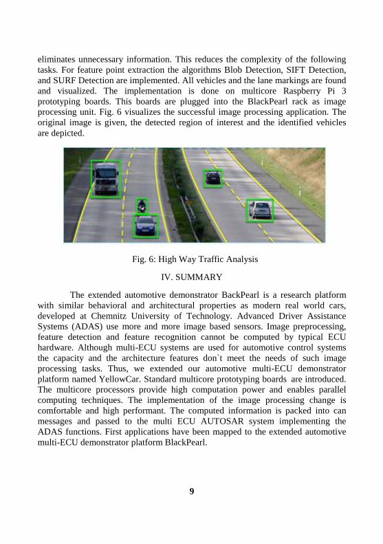
A typical CBIR system block chart is shown in Figure 1 :
22
Fig. 1. Typical CBIR system block chart
III. COMPARATIVE ANALYSIS OF THREE KINDS OF FEATURE
EXTRACTION ALGORITHMS
Compared with other image features, point feature has the virtue of little mount of account and great amount of image information. At the present stage, the research of local feature algorithm is mainly based on the extraction and matching of feature points. In this paper, the Harris algorithm, SUSAN algorithm and SIFT algorithm are compared and analyzed, and we have mainly discussed the SIFT algorithm.
A.Smallest Univalue Segment Assimilating Nucleus(SUSAN) algorithm
SUSAN is a simple and effective method to get feature points based on the gray value character. Firstly, move approximately circular template. In the image, make template core coincide and each pixel together; secondly, count the number of the similarity pixel between the template and the gray value to get the USAN value of and to calculate the corresponding value of the corner; finally, the feature extraction is implemented by using non maximum suppression method to calculate the feature point. This method is mainly used in edge-detection and corner–detection in image, and it is robust to noise interference. The SUSAN algorithm don’t need to segment the image, so there is no need to calculate the image gradient

23
data, at the same time, the USAN region is obtained by the pixel accumulation of similar gray value in the template and the center of the template, actually, in the process, the pixel accumulation is similar to the integral, from which Gauss noise can be effectively suppressed [5].
B.Harris Algorithm
Harris operator can give the autocorrelation matrix of a pixel in an image, which is inspired by the autocorrelation function in signal processing. And the characteristic value of autocorrelation matrix is the first order curvature of autocorrelation function [6]. Rectangular window w from the image to be processed to an arbitrary direction makes a slight displacement(x, y), then, the amount of change of gradation is calculated by the formula 1:
2
, , , ,
,
22 2
,
,
2 2
( )
2
=(x,y)M(x,y)
x y u v x u y v u v
u v
u v
u v
xy
T
E W I I
W xX yY o x y
Ax By C
(1)
Where M is the point (x, y) autocorrelation function matrix, and is the coefficient of gauss window. Judge whether the point is the corner by calculating whether the curvature value of XY two directions is high. However in the practical implementation of the algorithm, the trace and determinant of the matrix M are used to replace the eigenvalue for simplifying the calculation and improving the efficiency of retrieval. The algorithm has many advantages, including simple calculation, the feature of extraction point is uniform and reasonable. It can be quantitatively extracted feature points and it has better robustness for image rotation, brightness change, perspective changes and the effects of noise. However the scale is very sensitive, and it does not have the scale invariance and corner point extraction is the pixel level.
C.SIFT Algorithm
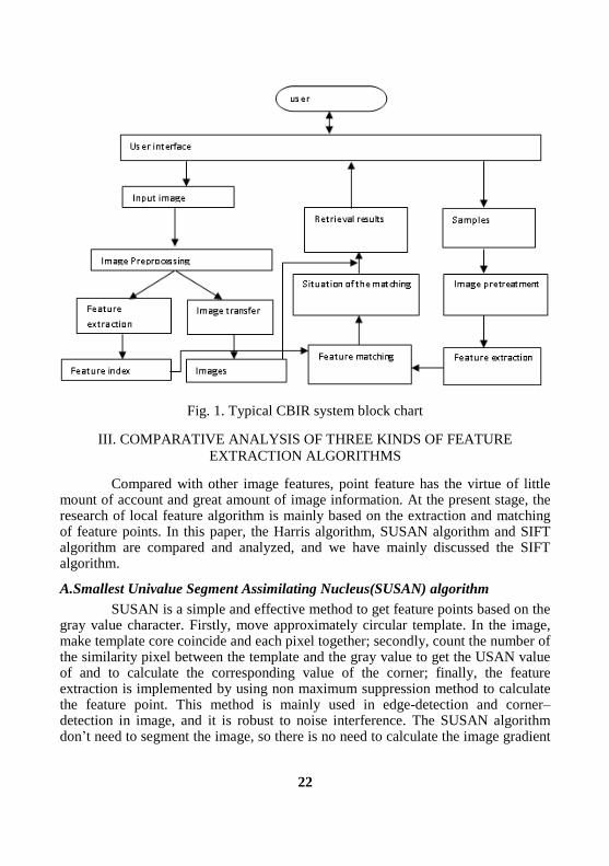
SIFT is a local feature description algorithm based on the scale space, which can keep invariant in the image transformation of scale, rotation and affine distortion. Describe the local features of the image, that is, the pixel gray gradient distribution in the vicinity of image feature points by establishing the DOG scale space, searching and locating the key points, and by feature points direction assignment and the key point descriptor. In order to verify the superiority of the SIFT algorithm, the performance test of SIFT is designed in this paper [7]. In the performance test, the feature points in the image are marked by green arrow, the direction of the arrow is the main direction of the feature point, and the length of
24
the arrow indicates the scale of the characteristic point [8]. It is clear that the SIFT algorithm has good robustness to scale changes, translation, rotation and brightness changes, but it has some limitations in the fuzzy retrieval for similar images [9,10]. The experimental results are as follows.

25
In addition to validate the point feature extraction, the feature extraction
and matching features and time were statistically tested in experiment. Limited
space, only a few groups of typical images of the experimental results are listed in
table Ⅰ:
TABLE 1: SIFT feature extraction and machine time of typical images
Number Type Thumbnail Feature
extraction time /ms
Matching time
/ms
Amount of
feature point
L1 Contrast
457 0 0
S1
Simple
Texture
457 <1 20
S2
471 1 32
M1
Medium
texture
541 5 139
M2
562
7
173
M3
541 7
203
F1
Complex
Texture
697 27 415
F2
963
277
1010

26
We use feature extraction time, matching time and amount of feature point
to compare the different type images. These results show that (1) SIFT feature
extraction capability is insufficient for low contrast image, as shown in l1, that (2)
SIFT has good feature extraction ability for the image with complex texture but
cannot get enough feature points for the image with simple texture and slow change
of gray value, as shown in F1 and F2, and that (3) SIFT spends a lot of time on
feature extraction, while feature matching time is very little, as shown in S1 and S2.
IV.CBIR SYSTEM BASED ON SIFT ALGORITHM
In this paper, a simple image retrieval system (iSee) was implemented in
the MATLAB. The system uses the query by example, takes SIFT algorithm as
feature extraction method and matches according to the distance-ratio criterion
using exhaustive method.
ISee system operation is divided into offline and online two processes. The
offline process is the generation and management of the image database feature
index. In this process, the system uses SIFT algorithm to extract the features of each
image in the original image database and generates feature information. The feature
information includes three parts: first, the image itself, second, the position, scale
and main direction information of the feature points, which is represented as a
vector set with K dimensional vector , and K is the number of feature points, and
third, the description vector of the feature points, which is represented as K vectors
with 128-dimensional. The online process is the image retrieval process. In this
process: First, some features are obtained from the object pictures. Second, match
the features in the retrieval index which is generated by the offline process. Finally,
display the result based on retrieval result. System can display pictures, where N is
for the number of the image database, P is for the confidence defined by the user,
and the proposed value is 0.01.
In this paper, we designed the corresponding iSee system image retrieval
experiment to test the performance of iSee.
In the experiment, join three types of pictures, each type with 10 groups
and each group with 20 pictures to form a picture library. There are the pictures X
such as the similar images, flowers, cars and so on. Also, similar texture images Y
and the images Z of the same object taken at different scales, viewing angles,
brightness and rotation angles. The images in the same groups have similar
characteristic and those in different groups are independence. From the image
database, select an image input into the iSee system to make an image retrieval as a
query image in each group of image. Then, statistical search results and statistical
results are shown in table Ⅱ.

27
TABLE II: Statistical results
The precision P and recall R can be calculated by following formula 2:
ARA C
APA B
(2)
Where A is the number of images to be retrieved and the number of images
similar to the reference image; B is the number of images that are retrieved but not
associated with the reference image; C is the number of images that are not
retrieved but similar to the reference image.
From table 1 statistical data shows, iSee retrieval ability is not good for X
images. It can only retrieve the query image itself and the images containing the
same object with the query image. Other results are returned as error results, and
only a few feature points are identified as the same feature points; For Y images,
the retrieval ability is some better than X image, but still not ideal, mainly because
the SIFT algorithm has trouble understanding and extracting features of the image
completely, so it is hard to match the same type but different characteristics of
images such as landscapes, flowers, cars and other visual. The visual features of the
texture include strategic line shape, color distribution, so it is difficult to produce
the similarity of the same with the human body for SIFT algorithm; For Z images,
SIFT algorithm shows its excellent retrieval performance, which can detect almost
all of the relevant images, that is associated with the SIFT algorithm. The image of
the scale, rotation, occlusion, perspective change, brightness and noise changes
have good robustness.

28
The SIFT algorithm is a favorable local feature descriptor, which owns a
good invariance to translation, scale, rotation, noise, angle change, and intensity
change. It is able to match the same object of two images accurately. These
properties of SIFT make it to have advantages over other algorithms in accurately
retrieving the target image. However, there is a huge limitation for SIFT when
implementing the fuzzy retrieval for similar images, which is shown in the
following figure.
Fig. 10. Matching result of similar images with SIFT
Figure 10 displays the matching result of two similar images with SIFT.
These are images of two marble bricks of the same kind. According to the figure,
we can get that although the two images are extremely similar, SIFT can hardly find
the same features (there are more than 5,000 features in both images, but none of
them are the same). The reason why SIFT is unable to find the same features is that
SIFT can only describe the low level visual feature, and cannot understand the
meaning of the image. Therefore, despite the fact that what shows on the images are
the same kind of object, the gray values of pixels around each feature are different
due to different backgrounds and object distributions. Consequently, SIFT
generates different feature descriptors, which is unable to detect the matching
features.
SIFT owns a huge advantage in some CBIR systems which need to
accurately retrieve the target image, such as fingerprint recognition, face
recognition, key frame retrieval, and medical image retrieval, etc. The sample
image of this kind of retrieving system has the same scene or object with the target
image, and only scale change, angle change or rotation happens. However, when it
comes to material retrieval which needs to retrieve the image that is in accord with
human’s judgment in visual and semantic aspects, SIFT does not seem to have a
good performance.

29
V. CONCLUSIONS
Based on the analysis of algorithm, a CBIR system based on the SIFT
algorithm was designed, and then an experiment proved the availability of the
system. Because the system has good robustness to scale changes, translation,
rotation and brightness changes, it has broad application prospects in the field of
accurate image retrieval, such as pattern recognition, face recognition, video key
frame search and medical image retrieval.
ACKNOWLEDGEMENT
This work was financially supported by National Natural Science
Foundation of China (Grant No. 61671190).
REFERENCES
[1] Chang T, Kuo C J. Texture analysis and classification with tree-
structured wavelet transform[J]. IEEE Transactions on Image Processing A
Publication of the IEEE Signal Processing Society, 1993, 2(4):429-441.
[2] Pentland A P, Picard R W, Scarloff S. Photobook: tools for content-
based manipulation of image databases[J]. Proceedings of SPIE - The International
Society for Optical Engineering, 1994, 2185:34-47.
[3] Jing F, Zhang B, Lin F, et al. A novel region-based image retrieval
method using relevance feedback[C]// 2001:28-31.
[4] Pass G, Zabih R. Histogram refinement for content-based image
retrieval[C]// IEEE Workshop on Applications of Computer Vision. IEEE
Computer Society, 1996:96. .
[5] Smith S M, Brady J M. SUSAN—A New Approach to Low Level
Image Processing[J]. International Journal of Computer Vision, 1997, 23(1):45-78. .
[6] Harris C. A combined corner and edge detector[J]. Proc Alvey Vision
Conf, 1988, 1988(3):147-151.
[7] Lowe D G, Lowe D G. Distinctive Image Features[J]. 2004.
[8] Zhu Y, Li J, Yang W, et al. A feature points description and matching
algorithm for edge in IR/visual images[J]. Jisuanji Fuzhu Sheji Yu Tuxingxue
Xuebao/Journal of Computer-Aided Design and Computer Graphics, 2013,
25(6):857-864.
[9] Ma J. A scene matching approach based on edge signal between
IR and visible image[D]. The Huazhong University of Science and Technology,
Wuhan, China, 2006.
[10] Wang S. SIFT based image matching algorithm research[D].
Xidian University, Xian, China, 2013.

30
Decoding of digital holograms
Vladimir I. Guzhov1, Ekaterina E. Serebryakova
2
1,2Novosibirsk State Technical University (NSTU)
[email protected], [email protected]
2
Abstract - The article describes a system for recording digital
holograms. The Fresnel transformation is used for decoding.
Keywords - holography, optical microscopy, interference, digital
holography, Fresnel transform, Fourier transform.
I. INTRODUCTION
To register classical thin holograms it is necessary to use high-resolution
photographic media. This is due to the fact that when the real and imaginary images
are restored they overlap with the central beam. E. Leith and Yu. Upatnieks solved
the problem of separation of beam overlap as follows [1]: they directed an object
beam of light onto a photographic plate at a rather large angle with a beam of light
diffracted by the object; this made it possible to obtain images that, when observed,
do not overlap. To record a hologram at an angle between interfering strips of 30
degrees, a recording material with a resolution of at least 2000 lines / mm is
required for recording only the carrier frequency.
Digital matrices used in digital holography can't at the moment provide
such a high spatial resolution. Therefore, in digital holographic reconstruction, it is
necessary to reduce the angle between the interfering wave fields, which inevitably
leads to overlapping of the spectra in different diffraction orders.
II. THEORY
The existing methods for decoding holograms are based on the fact that we
can register only the intensity of the hologram. However, in contrast to recording
classical holograms that represent a picture of intensities, using digital holography
one can obtain a complex mathematical hologram [2], which consists of the
amplitude and phase of the object field:
( , ) ( , )exp ( , )p pG x y a x y x y (1)
( , )pa x y - field amplitude, ( , )p x y phase of the field propagated from the object
in the plane of the hologram ( , ) .

31
The amplitude and phase values can be found from the set of holograms
using phase-shifting interferomet The stepwise phase shift method is based on recording several interference
patterns when the reference wave phase changes by a certain amount. The phase
shift between interfering beams can be realized in various ways. The phase shift is
most often set using a mirror fixed to a piezoceramic. Depending on the number of
phase shifts, there are various decoding algorithms.ry (PSI) methods.
In [3] it is shown how to obtain computational procedures which, using
combinations of intensity of interference patterns, obtain the distribution of the
phase difference ( , )x y of interfering beams for arbitrary angles of displacement. In
[4-6], a generalized scheme of the algorithm for a different number of shifts is
obtained. Knowing the phase difference ( , )x y and the phase of the reference wave
( , )r x y , it is possible to determine the initial phase distribution ( , )p x y .
( , ) ( , ) ( , )p rx y x y x y (2)
To form a mathematical hologram it is also necessary to determine the
amplitude of the wave field ( , )pa x y reflected from the object in the plane of the
hologram. The values of the amplitudes of the object and reference beam can be
determined by overlapping the corresponding beams in the optical circuit. But if we
already have a set of registered holograms with a phase shift used to determine the
phase values, then we can obtain the amplitude of the object beam by the stepwise
shift method using the same set of holograms [7,8].
If you can find a mathematical hologram ( , )G x y , then in the image plane
you can restore the complex amplitude of the field scattered from the object. For
this, it is necessary to carry out the Fresnel transformation over ( , )G x y [9].
2 2
112 2
1
( ) ( )1 2( , ) exp
2( , )exp exp
yxNN
k l
r sdr s exp i i
i d d
b k l i k l i kr lsd N
(3)
In expression (3), d - the distance to the object. The Fresnel transformation
algorithm provides a simple scaling of the reconstructed image, but this imposes a
number of limitations on the design of the measuring system, in particular, the
upper and lower limits of the permissible recording distance of the hologram
become a significant factor.

32
It is necessary to determine at what distances we can use the discrete
Fresnel transform. It was shown in [10] that discrete Fresnel and Fourier transforms
can be used when the distance to the object is comparable with the size of the object
and hologram, while the object is in the near zone of diffraction. When recording
digital holograms, the optical scheme shown in Fig. 1.
Fig. 1. Scheme of recording a digital hologram
The beam of light from the laser expands (3) and hits the separation cube.
Part of the beam hits the mirror fixed to the piezoceramic (5). When reflecting from
this mirror, an object beam is formed. Another part of the beam hits the object.
When reflecting from the object (2), a reference beam is formed. To equalize the
intensities of the reference and object beams, a light filter is used to form the
hologram (4). The interference of the reference and object beams and the formation
of holograms occurs on the camera array (9).
III. EXPERIMENTS AND RESULTS
The object was a jubilee silver badge with the emblem of the university. In
Fig. 2 shows the results of interference between the reference and object beams
when the phase angle of the shift is changed . Interference patterns were projected
directly onto the digital array of photodetectors.
Figure 2. Interference patterns with a change in the phase angle of shear
1 2 3 30 , 90 , 180 , 270

33
For these pictures, the phase distribution and amplitude were determined.
Then a mathematical hologram was formed using the expression (1). In Fig. 3
shows the amplitude and phase of the mathematical hologram.
Figure 3. Amplitude and phase of the mathematical hologram.
The actual image was reconstructed from the mathematical hologram using
the Fresnel transform. The size of the object is 7 mm, the distance to the object is
135 mm. The result of the restoration is shown in Fig. 4.
Figure 4. Left source object, right: the result of restoring the actual image
from the mathematical hologram.
The noise in Fig. 4 are caused by the deflection of the reference beam from
the plane beam. By improving the quality of optical elements, this factor can be
eliminated.
This work was supported by the Russian Foundation for Basic Research
"Development and research of computer holographic interferometry methods for
complex objects" (Grant No. 18-08-00580).

34
REFERENCES
[1] Leith, E.N. Reconstructed wavefronts and communication theory
[Text] E.N. Leith, J. Upatnieks. Journal of the Optical Society of America, 1962,
Vol. 52, pp. 1123-1130.
[2] YAroslavskij, L.P. Cifrovaya golografiya [Tekst]. L.P. YAroslavskij,
N.S. Merzlyakov. – M.: Nauka, 1982, P. 219 .
[3] Guzhov V.I., Il'inyh S.P. Opticheskie izmereniya. Komp'yuternaya
interferometriya: Ucheb. posobie. - Moskva: Izd-vo YUrajt, 2018. (ISBN: 978-5-
534-06855-9), P.258.
[4] Guzhov V., Ilinykh S., Kuznetsov R., Haydukov D. Generic algorithm
of phase reconstruction in phase-shifting interferometry. Optical Engineering, 2013,
Vol.52(3), pp. 030501-1 – 030501-2.
[5] Guzhov V.I., Il'inyh S.P., Hajdukov D.S., Vagizov A.R. Universal'nyj
algoritm rasshifrovki. Nauchnyj vestnik NGTU, 2010, 4(41), pp. 51-58.
[6] Il'inyh S.P., Guzhov V.I. Obobshchennyj algoritm rasshifrovki
interferogramm s poshagovym sdvigom. Avtometriya, 2002, 3, pp.123-126.
[7] Guzhov V.I., Il'inyh S.P., Hajbulin S.V. Vosstanovlenie fazovoj
informacii na osnove metodov poshagovogo fazovogo sdviga pri malyh uglah
mezhdu interferiruyushchimi puchkami. Avtometriya, 2017, T. 53, 3, pp. 101-
106.
[8] Guzhov V.I., Il'inyh S.P. Opredelenie intensivnosti opornogo i
ob"ektnogo puchkov pri ispol'zovanii metoda poshagovogo fazovogo sdviga.
NGTU, Novosibirsk, Rossiya. Avtomatika i programmnaya inzheneriya, 2017, 4
(22), pp. 68–73.
[9] Predstavlenie preobrazovaniya Frenelya v diskretnom vide. Guzhov
V.I., Nesin R.B., Emel'yanov V.A. Avtomatika i programmnaya inzheneriya,
Novosibirsk, 2016, 1(15), pp. 91–96
[10] Oblast' vozmozhnogo primeneniya diskretnyh preobrazovanij Fur'e i
Frenelya. Guzhov V.I., Emel'yanov V.A., Hajdukov D.S. Avtomatika i
programmnaya inzheneriya, Novosibirsk , 2016. 1(15), pp. 97–103

35
Video-based fall detection system in FPGA
Peng Wang1, Fanning Kong
2, Hui Wang
3
1,2,3 Harbin University of Science and Technology (HUST)
- [email protected], [email protected]
3
Abstract—As there is a high tendency of falling in the independent
living of the elderly and the post-fall injury is very serious. It is necessary to
get timely assistance when they fall down. The main objective of this work is to
build an FPGA-based hardware implementation of video-based fall detection
system. First of all, the moving object model will be extracted through
background subtraction based on Gaussian Mixture Models (GMM). Second,
we judge whether there is a fall through the aspect ratio, the effective area
ratio, and the change in the center of the human body. Finally, the detection
system will make sound-light alarm and send messages to the elder’s family
and the community via GSM when they fall down. The experimental results
demonstrate the accuracy of this fall detection system is up to 95% and this
system satisfices the requirement of real-time, low rate of false positives and
good robustness.
Keywords—Fall detection, FPGA, Video-based, Background
subtraction, GSM
I. INTRODUCTION
With the global aging population grows tremendously, large part of elderly people has to live alone while their children work outside. As reported that 28-35% from age group 65-75 falls at least once a year [1]. Falling exposes the elder to greater chances of suffering fall-related injuries [2]. Therefore, it is essential to put forward an automatically fall detection system for enabling the falling elder get immediate help to avoid any post-fall injuries or deadly cases due to delayed assistance.
While various kinds of fall detection system have been researched in recent years, research in video-based fall detection has gained much attention [3]. Most of video-based fall detection which are implemented on the general purpose CPU or PC with software processing not targeting for real-time [4,5]. FPGA has advantages over CPU and PC because of the large number of processing cores that work in parallel in FPGA. It has proposed a video-based fall detection system, in this work, which FPGA is selected as an accelerator to improve the performance of the system.

36
The followings are the organization of this paper. The overall concept of the system is described in Chapter 2. In Chapter 3 the fall detection algorithm is explained. Chapter 4 discusses the implementation on FPGA. At the end, results and conclusions are presented.
II. OVERVIEW OF THE SYSTEM
The presented system consists of a digital camera, an automatic detection
platform with Cyclone IV FPGA device (EP4CE15F17C8N), LEDs, a Buzzer and a
GSM module. All computation of the system should be done inside the FPGA and
the alerts will happen together with LEDs, Buzzer and GSM. The idea is described
in Figure 1. The system is based on the following elements: Digital camera with
OV7725 from OmniVision for capturing the video streaming,
The automatic detection platform with Cyclone IV FPGA device from
Altera, which as the main computing platform, carries out all image processing and
fall detecting operations,
LEDs and Buzzer for giving an alarm of light and sound to caution the
neighbors, the LEDs also could be used as the lighting in daily life,
GSM module for sending the falling messages to the falling elder’s family
and the community.
OV7725
Camera
Automatic
detection system
with FPGA device
LEDs
Buzzer
GSM
Fig. 1. Overview of the fall detection system
III. FALL DEECTION ALGORITHM
A number of algorithms for object detection have been presented. Object
detection algorithms can be classified into Frame subtraction schemes, Optical flow
method and Background subtraction. The algorithm of Frame subtraction schemes
is easily influenced by the time interval that could not extract the full foreground.
The disability of Optical flow method is complex computation which leads bad
real-time performance. In this work, we choose the Background subtraction with its
simple principle and computation. Figure 2 shows the process of Background
subtraction. The behavioral simulation results were completely compliant to
software model created in Matlab R2012a.

37
Read frameBackground
generation
Background subtraction
Object Detection
Image binaryzation
Minimum bounding box
Aspect ratio
>T1?
Effective area ratio
>T2?
body center
>T3?
Fall detection
Y
Y
N
N
Fig. 2. Flow chart of the fall detection algorithm
A. Background generation
In this work, GMM (Gaussian Mixture Background Modeling) was adopted for background generation. Every single pixel was expressed the feature with Gaussian model according to the following Equation 1:
1, ,
1
2, , 1
22,
1, ,
2
T
t i t i i tx u x u
i t i t i t n
i t
F x u e
(1)

38
Then the background model was built with the weighted sum of the K - Gaussian models by the Equation 2:
, , ,
1
, ,k
t i t i t i t i t
i
P x w F x u
(2)
B.Moving object segmentation
After background generation, the next step was classifying the pixels into foreground object as the Equation 3 shows:
, ,N BI x y I x y T (3)
while at coordinate (x, y), IN (x, y) is the intensity value for the new pixel; IB (x, y) is the intensity value for the background pixel; T is a difference threshold which is pre-determined. Meanwhile, the pixel will be classified as the background object if the condition in Equation 3 is not fulfilled.
C.Fall detection
The minimum bounding box was generated with its features (height, width
and size) for foreground object following the image binarization. As we know, a
standing person should have a height (H) greater than width (W). It turns out to a
height to width ratio (aspect ratio) > T1, which T1 is the threshold, as shown in
Figure 3a. On the contrary, a person who is falling should have an aspect ratio < T1,
as illustrated in Figure 3b. In spite of that, this work has proposed the
supplementary condition to distinguish the real-fall from the daily exercises by the
effective area ratio as shown in Equation 4.
Oeffective
B
SR
S (4)
Where SO = the area of the foreground object; SB = the area of the
bounding box. It will be detected as a fall if the Reffective greater than T2. T2 is the
threshold that predetermined.
Because normal movement is slow and the center changes little when the
old man squats, push-ups or walks normally. Fall is a kind of rapid and violent
phenomenon. During the fall down, the change of the center will suddenly increase.
Finally, in order to further improve the accuracy of the system, the judgment results
are corrected according to changes in the body center. After calibrating the
minimum external bounding box of the human body, find the center position O(x, y)
of the human body, and correct the fall judgment result by using Equation 5:

39
1
2 2
1 1 3
,y y
y y x x
k k
k k k k
O O
O O O O T
。
(5)
Compare human body centers Ok(x,y) and Ok-1(x,y) of two adjacent images.
When the center of the human body in the k-th frame image is lower than the body
center in the k-1 frame image. And the distance between the two centers is greater
than the threshold T3, the result of the determination is a fall. Otherwise, it is not a
fall.
(a) Person standing (b) Person falling down
Fig. 3. Aspect ratio, effective area ratio and body center of bounding box
IV. IMPLEMENTATION ON FPGA
In this work, it has proposed a hardware implementation of fall detection
system using FPGA. Figure 4 has shown the functional diagram of the system
implemented in FPGA. Most important are:
CMOS sensor config - block for configuring the COMS sensor,
Image capture - reading the video streaming received from CMOS
sensor,
RAW2RGB - module for changing the color space from RAW to RGB,
SDRAM controller - hardware SDRAM memory controller.
Write FIFO/Read FIFO - write the image frames to SDRAM or read
the image frames from SDRAM,
SRAM controller - registers holding parameters for the fall detection
algorithms,

40
Algorithms - this part mainly conclude: background generation,
background subtraction, mini-mum bounding box and fall detection,
LED controller - controlling the LEDs with flashing for alarm when a
fall happened,
BUZZER controller - realizing the audible alarming along with the
LEDs flashing, so that could alert neighbors when a fall is detected,
GSM controller - controller for sending falling messages to ensure the
victim got timely assistance.
CMOS
sensor
CMOS sensor
config
Image capture
RAW2RGB Write FIFOSDRAM
controller
SDRAM
Read FIFO
Background
generation
Background
subtraction
Minimum
bounding box
Fall detection
LED BUZZER GSM
SRAM controllerSRAM
FPGA
LED
controller
BUZZER
controller
GSM
controller
Algorithms
Fig.4 Overview of the fall detection system
Firstly, the CMOS sensor was configured through a configuration block.
The FPGA acquired the video streaming through a capturing module from the
CMOS sensor. Then, change the raw data from Bayer format to RGB format
through a conversion module. The video frames and the generated background
models were stored in the SDRAM with the FIFOs. To detect the moving object,
the new image frame and background model will be read together in pixels from the
SDRAM. The foreground model was generated by setting their absolute difference
threshold. Finally, the FPGA will drive the alarm controller after a fall event being
determined with the bounding box.
The project was synthesized for an Altera Cyclone IV (EP4CE15F17C8N)
FPGA device using Quartus II Design Suite. The behavioral simulations performed

41
in ModelSim 10.0c verified that the hardware modules are fully compliant with the
software described in Matlab R2012a. Table 1 presents the resource usage of the
FPGA.
It is worth noting that the data from Table 1, even a small FPGA device
from Cyclone IV series can run quite complex video-based fall detection system
which resource utilization at about 35% of the available resources.
TABLE I. Project resource utilization
Resource Used Available Percentage
FF 5457 54576 10%
LUT6 5730 27288 21%
LE 4922 15408 32%
DSP48 54 112 48%
BRAM 22 116 19%
V. IMPLEMENTATION ON FPGA
An Altera Cyclone IV (EP4CE15F17C8N) FPGA device is used to
implement the presented fall detection system. The implementation was made using
Verilog HDL hardware description language. The same fall detection algorithm was
implemented in Matlab for benchmarking purposes using C programming language
on a PC which contains Intel Core i3-4170 3.70 GHz CPU with 4GB RAM.
(a) standing (b) squatting

42
(c) lying down (d) leg pressing
(e) falling down (f) doing push-ups
Fig.5. Fall detection with Aspect ratio and Effective ratio
After repeated experiments, we took 1.2 as the aspect ratio threshold. Using
0.45 as the effective area ratio threshold and 6.5 as the body center threshold in this
work.
Take the first 1000 image frames of the video stream for the tests. Figure 5b,
Figure 5c, Figure 5d, Figure 5e and Figure 5f were detected as fall events just with
the aspect ratio, which were shown in Figure 5. Figure 5b, Figure 5d and Figure 5f
were misjudgments for doing daily exercises such as squatting, leg pressing, doing
push-ups and so on. Therefore, this work introduces effective area ratios and center
changes as corrections for falls. This can improve the accuracy of the fall detection.
A. Accuracy of the System
A large number of tests were conducted to assess the accuracy of the fall
detection system. Table 2shows the results of the tests. The true positive of the
FPGA-based solution is 2% lower than the Matlab-based solution. This result could
be simply because of the processing speed of FPGA is much faster compared to
Matlab.

43
TABLE II. Fall detection rate for both FPGA and Matlab implementations
Platform True
Positive
True
Negative
False
Positive
False
Negative
FPGA 96.00% 94.46% 5.54% 4%
Matlab 97.00% 93.56% 6.44% 3%
1) Ture Positive = correctly detected the number of falls/the actual total number of falls.
2) Ture Negative = number of normal activities detected / total number of normal activities.
3) False Positive = number of falls judged by mistake / total number of normal activities.
4) False Negative = No number of falls detected / Total number of actual falls.
Table 2 shows that the FPGA platform's fall detection accuracy is 1%
lower than the Matlab platform. The result may be due to the FPGA processing
speed is too fast. Causes the loss of image frames. This is where this article needs to
continue to improve
B. Processing Frame Rate
The processing frame rate of the implemented system was evaluated and is
shown in Table 3. The results give a value of 56.36 fps with the resolution 640×480.
The number of clock cycles required to complete a frame of image processing by
the test system algorithm to calculate the frame rate of the video. In the meantime,
the time required for Matlab to conduct the same image frames processing was
calculated. The results demonstrate that the performance of video based fall
detection in FPGA is near to 6X faster than the Matlab-based implementation.
TABLE III. Detection time for a single frame on the FPGA and Matlab
Platform Max.(s) Min.(s) Avg.(s) Frames per second(fps)
FPGA 0.017 0.017 0.017 56.36
Matlab 0.128 0.076 0.099 10.10
C. System alarm time
The average time of audible and visual alarm response in Table 4 is 0.51s.
The time for sending GSM messages is often influenced by cell phone signals or
network operators. the average time of GSM message sending time is 4.97s. The
experimental results prove that the real-time nature of the fall detection alarm
system based on FPGA can meet the system requirements.
44
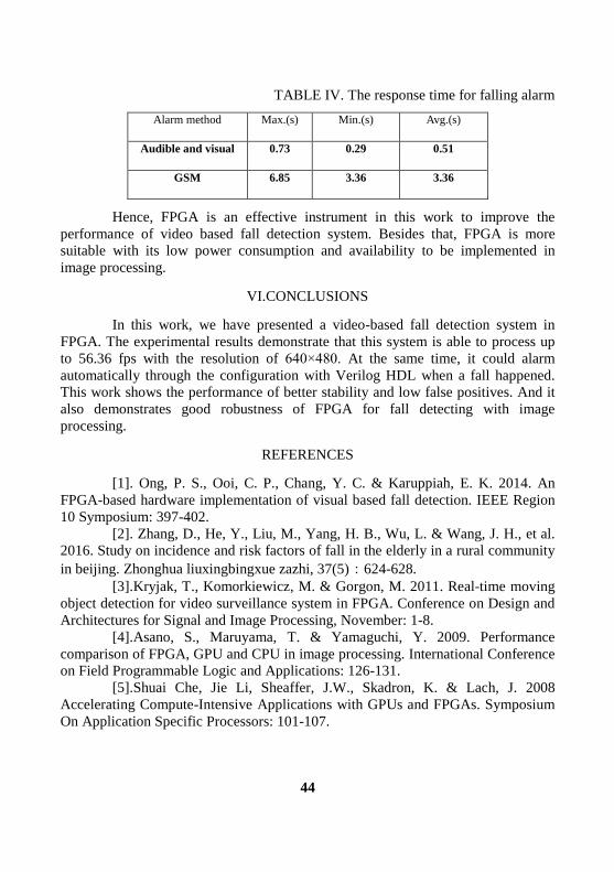
TABLE IV. The response time for falling alarm
Alarm method Max.(s) Min.(s) Avg.(s)
Audible and visual 0.73 0.29 0.51
GSM 6.85 3.36 3.36
Hence, FPGA is an effective instrument in this work to improve the
performance of video based fall detection system. Besides that, FPGA is more
suitable with its low power consumption and availability to be implemented in
image processing.
VI.CONCLUSIONS
In this work, we have presented a video-based fall detection system in
FPGA. The experimental results demonstrate that this system is able to process up
to 56.36 fps with the resolution of 640×480. At the same time, it could alarm
automatically through the configuration with Verilog HDL when a fall happened.
This work shows the performance of better stability and low false positives. And it
also demonstrates good robustness of FPGA for fall detecting with image
processing.
REFERENCES
[1]. Ong, P. S., Ooi, C. P., Chang, Y. C. & Karuppiah, E. K. 2014. An
FPGA-based hardware implementation of visual based fall detection. IEEE Region
10 Symposium: 397-402.
[2]. Zhang, D., He, Y., Liu, M., Yang, H. B., Wu, L. & Wang, J. H., et al.
2016. Study on incidence and risk factors of fall in the elderly in a rural community
in beijing. Zhonghua liuxingbingxue zazhi, 37(5):624-628.
[3].Kryjak, T., Komorkiewicz, M. & Gorgon, M. 2011. Real-time moving
object detection for video surveillance system in FPGA. Conference on Design and
Architectures for Signal and Image Processing, November: 1-8.
[4].Asano, S., Maruyama, T. & Yamaguchi, Y. 2009. Performance
comparison of FPGA, GPU and CPU in image processing. International Conference
on Field Programmable Logic and Applications: 126-131.
[5].Shuai Che, Jie Li, Sheaffer, J.W., Skadron, K. & Lach, J. 2008
Accelerating Compute-Intensive Applications with GPUs and FPGAs. Symposium
On Application Specific Processors: 101-107.

45
Security of Users in Cyberspace
Ivan L. Reva
Novosibirsk State Technical University(NSTU)
Abstract - Recently, telecasts, video clips and news lines on the Internet
include such words as "information wars, hackers, cyber weapons, viruses ...".
Ten or fifteen years ago, such phrases could only be heard in fantastic films. In
the age of rapidly developing information technologies, WWW (Internet),
social networks and information resources, IT-technologies are widespread in
all of society's life areas. The virtual world is becoming more realistic, now a
modern person, typically, has two lives – so-called "material" and "virtual".
And if the material life is governed by laws and society traditions, the virtual
one has no legal framework; it creates its own unspoken rules, which affect
modern society. The virtual world has no border, that is why countries cannot
completely control it with laws. The problem is still up-to-date and many IT-
specialists try to find solutions. The need for common rules that would allow
finding violators of the behavior standards in this area is obvious, but it is not
easy to make the united rules for everyone, because laws in different countries
differentiate one from another. However, it is still possible to find a general
solution, there are things that unites all - for example, dislike for spam and
viruses (except for those who receive money from this harmful activity).
Keywords - user security, cyberspace, information security.
I. INTRODUCTION
Now almost all international organizations have groups that deal with the
development of laws regulating work in cyberspace that are acceptable for most
countries. At moments of danger, humanity still knows how to negotiate, so I think
that this task is quite feasible. [1]
The scale of influence of Information Technologies industry on the state
exceeds only partial effects. Development of Information Technologies is one of the
most important tasks of the Russian Federation. According to the online news
edition RIA Novosti, the number of Russian Internet audience exponentially
growing (Fig. 1 a,b). [1] In Russia, the number of information services has
increased significantly, both on a commercial and state level. But with development
of information services, the number of cyber-attacks on the servers of Russian
companies is also increasing. So according to Kaspersky Lab's (Fig. 2), in 2016

46
Russia took the fourth place in the World in terms of the number of cyber attacks.
[2]
Fig. 1a. The Global Internet users number
Fig. 1b The Russian Internet users number

47
Fig. 2 Cyber-attacks geography
This is not surprising, because by the beginning of 2007 hacking became
commercial, what lead to competition in this sphere, which contributed to the rapid
growth of the quality of malicious software products and decrease of prices for
services in this field. The growing number of hacked machines all over the world
makes us talk about an industrial revolution in this sphere. On the one hand, it has
become one of the most important types of criminal business, on the other - the
level of organization, automation and division of labor in this industry have reached
an unprecedented scale.
According to experts, more than 140 countries around the world develop
cyber weapons, which are characterized by their secrecy and economic efficiency.
Therefore, the number of operations in cyberspace is constantly growing: thousands
of attacks are carried out daily throughout the world aimed at disrupting operation
of state and commercial infrastructure of different countries.[1]
Obviously, in the pursuit of IT implementing, humanity faced a number of
problems. The key problem was the safety of users in cyberspace, only in some
social networks there is a huge amount of personal information, such as:
FULL NAME;
Date and place of birth;
Place of residence;
School number;
Phone number;
Names, photos and contacts of family and friends;
etc.

48
The users of the Russian Federation public services portal
(www.gosuslugi.ru) perfectly know what data is stored in their personal cabinets,
use of banking online services and so on. It is not even possible to imagine the
consequences of the leakage of this data into the hands of intruders.
Another not less important problem of informatization of the society is its
influence on development of the younger generation. Impact of malefactors on
children through the worldwide network is well-known, and sometimes the
situations end up tragically. Propaganda and false information into the network can
affect even the consciousness of an adult. The listed problems are so serious that
they need to be solved at the state level.
What can we do? How to protect yourself in the virtual world? Typically,
the society is not competent in these matters, and sometimes underestimates the
threats. In fact, to protect yourself is not so difficult. Everyone remembers from an
early age, what is good and what is bad, how we were taught a healthy lifestyle, so
that we would not get sick, everyone remembers these simple rules:
Brush your teeth when you are woke up;
Do exercises;
Wash hands before eating;
Eat three meals a day;
Do sport;
etc.
There is the similar situation in virtual world: you need to remember the simple
rules and try to follow them.
II. RULES FOR ENSURING THE SAFETY OF TEENAGERS IN CYBERSPACE
In order to form and develop the ability to use safe information and
communication technologies and use the virtual pace competently, one
must adhere to the following rules:
Stimulate and warn teenagers that they need to place their personal
information on the Internet carefully;
Tell them about a possible threat from strangers, especially in chat rooms
and social networks;
Teach a teenager how to act when unpleasant materials appear and close
such Web sites;
Regularly remind that information on the Internet is not always reliable;
Do not disclose your passwords and periodically change them.
To ensure effectiveness of the teenager protection in a network , you need
to install security filters on your computer to protect it from viruses and
spyware. If necessary, consult with specialists.

49
III. RULES FOR ENSURING THE PERSONAL SAFETY IN CYBERSPACE
As mentioned earlier, the human life is impossible without IT technologies,
almost everyone has a personal computer with Internet access in which a user stores
their data, performs any work, purchases goods. We must take steps to protect data.
There is a list of actions which can help you to make your Internet activity safer:
Try to copy all important information to removable media.
Do not place a lot of information in social networks.
To make purchases through the Internet use a debit rather than credit cards.
(It is advisable not to store large sums of money on plastic cards).
Do not download software from unknown vendors.
In mail services, do not start .exe files from unknown recipients.
The optimum length on passwords is 7 -8 characters.
Do not click the pop-up windows. It is better to close such resources
immediately. (I recommend blocking pop-ups in the browser settings.)
It is not recommended to insert a personal USB - flash drive in unfamiliar
computers.
Try to use licensed software.
These simple rules would help you to avoid any problems in cyberspace.
Please, take care about your personal data.
REFERENCES
[1]. RIA news [Electronic resource] URL: www.ria.ru. – Title from screen.
[2]. DDOS-attacks on networks in contemporary world [Electronic
resource] URL:https://securelist.ru/analysis/malware-quarterly/30152/ddos-attacks-
in-q4-2016/. – Title from screen.
[3]. Informatics[Electronic resource] URL: http://ppt4web.ru/informa tika.
– Title from screen.

50
Feature-based Image Processing Algorithms for Vehicle
Speed Estimation
Reda Harradi 1, Ariane Heller
2, Wolfram Hardt
3
1,2,3TU Chemnitz
3wolfram.hardt
@cs.tu-chemnitz.de
Abstract—The aim of this paper is to implement a filter-based
software solution for detecting vehicles from a set of videos and estimating
their speeds. The proposed implementation utilizes a set of low-level filters for
extracting different regions of interest that depict the initial motion of each
detected vehicle. Different approaches are then proposed to extract stable low-
level features; either using the Shi-Tomasi algorithm, the Scale Invariant
Feature Transform (SIFT) algorithm or the Speeded- Up Robust Features
(SURF) algorithm for enabling the further tracking. The tracking of those
aforementioned low-level features is then performed using the Kanade-Lucas-
Tomasi (KLT) algorithm. The speeds of the vehicles are then calculated by the
means of an Inverse Perspective Mapping, and by projecting the traveled
displacements of the tracked features to known real world measures, in order
to be able to change the measurements’ unit system of the calculated vehicles’
speeds from pixels per second to kilometers per hour.
Furthermore, the implementations were done on the Automotive Data
and Time-triggered Framework (ADTF) from Elektrobit, which provides the
possibility of having a good modularity of algorithmic models for image
processing. The testing was based on a dataset of videos provided by the
research project done by Luvizon et al. at the Federal University of
Technology in Parana, Brazil, on proposing a novel vehicles’ plates detector,
where almost five hours of videos were captured in different conditions by a
single low-cost digital camera, placed at meters from the ground. The
provided dataset contains more than 8 thousand vehicles and is associated
with a ground truth reference obtained through the use of a state-approved
inductive loop detector, that provides the real world speed measures of almost
all the vehicles within the dataset.
Keywords—ADTF, Feature Extraction, Feature Tracking, Shi-Tomasi, SIFT,
SURF, KLT.
I. INTRODUCTION

51
Preventing road accidents has always been a major field of research within
the automotive industry. Sadly, nearly 25,300 people departed this life and another
135,000 people were seriously injured or left with life-changing injuries on the
European roads in 2017, according to the recently published data on Road Safety
that is pursued by the European Commission based in Brussels. In fact, the rate of
death on European roads has dropped down by 2 % compared to 2016, and has
showed the same decreasing trend as in the previous year. The study also showed
that of all the road accidents, 8 % occurred on motorways, 37 % in urban areas, and
55 % in rural areas [1].
While these numbers still hide stories of pain and grief, the European roads
remain amongst the safest in the world. With 49 road casualties per one million
inhabitants, against 174 mortalities per million worldwide, the European Union has
made a substantial improvement in reducing the number of road accidents over the
past twenty years. A part of this progress was thanks to the establishment in 2010 of
the Road Safety Programme 2011-2020, that came up with European and national
level orientations with the aim of cutting by half the ratio of traffic deaths in Europe
by 2020 [1].
This paper falls within two of the main building pillars of the Road Safety
Programme 2011-2020, which are building safer road infrastructures and boosting
smart technologies. The program aims at introducing new active safety measures
for safety equipment, extending the existing legislations to cover the rural roads as
well, and speeding the new technical projects for enabling the data and information
exchange between the vehicles and the road infrastructures. As a matter of fact, this
paper is motivated by the desire of using normal electro-optical sensors present in
modern-day cameras to detect, classify and recognize vehicles present within an
urban road traffic. The goal is to tackle the issue of detecting the vehicles’ speeds
in urban areas at reduced costs; by the means of image processing instead of relying
on currently used specialized-sensing technologies, e.g., ultra-sonic sensors, loop
detectors, etc.
II. PROPOSED APPROACH
The main methodological approach in this paper is com- posed of a six-
stages processing chain, as depicted in Figure 1. The processing chain starts with a
pre-processing step, which consists of first applying a set of pre-processing filters
on the input video frames, in order to provide a noise-free base that would facilitate
the further processing.
The second step is then responsible of deriving the contours and convex
hulls shapes of the vehicles present within each frame. Once accomplished, the next
step of the processing, which focuses on the multiple separate regions of interests

52
(ROIs) given by the convex hulls, continues the processing chain thence, where the
low-level features extraction mechanisms allow the extraction of the feature
keypoints describing the vehicles of interest. Note that in this approach, only one
low-level feature extractor is used at a time, i.e., either Shi-Tomasi, SIFT, or SURF.
A comparison of the results of using each different extractor is given in section IV.
The vehicles are then classified, depending on their sizes and aspect ratios, into
either motorbikes, cars, or trucks, to be then tracked throughout the whole sequence
of the video frames in which they appear, through the use of the Kanade-Lucas-
Tomasi (KLT) algorithm. Finally, the process ends with a scene interpretation,
where an Inverse Perspective Mapping (IPM) projection is applied, in order to
estimate the detected vehicles’ speeds, not only in pixels per second, but also in
kilometers per hour.
Fig. 1 – Diagram of the processing flow chain of the main methodological
approach used in this paper

53
III. IMPLEMENTATION
The implementation of the system has been done in accordance with the
Automotive Data and Time-triggered Frame- work (ADTF) version 2.13.1 from
the Elektrobit company. This framework allows several benefits for the evaluation
and validation of software algorithms. It consists of a well-defined software
development kit (SDK) for the C++ programming language, an organized graphical
configuration editor, and a suite of pre-defined toolboxes for various purposes,
such as the Video Compression Toolbox, that manages the compression and
decompression of the video streams used within ADTF, and the Device Toolbox,
which ensures the connection to several types of external devices, e.g., CAN, LIN,
FlexRay, MOST and Ethernet bus systems, and the Display Toolbox, that provides
pre-defined Filters for various displaying and rendering purposes.
Furthermore, the choice of ADTF as a developing frame- work is justified
by the fact that it offers the support for implementing new functions in a fast,
prototypical and incremental way. Additionally, ADTF offers a layered architecture
that enhances the modularity of the implemented software solutions, in such a way
that the modules, i.e., filters, are freely changeable and expendable.
Fig. 2 – Figure showing the overall architecture of ADTF. Figure adapted
from [2]
As a matter of fact, ADTF is based on a layered architecture, as depicted
in Figure 2. The architecture consists of four main tiers: The Micro Component
54
Object Model (µCOM), which is the base layer; based on the Microsoft
Component Object Model, and is responsible of defining the components, the
basic interfaces and the inter-process communication, as well as the components’
interactions. Next comes the µCOM Runtime layer, where the plugins that are
managing the interactions between the different modules could be loaded,
registered, and deregistered. Moreover, the ADTF Services layer consists of
defining the various system services provided among the functionalities of ADTF
itself. Those services, e.g., memory management, project loading and management,
etc., remain throughout the whole running cycle of ADTF, i.e., from the start-up of
ADTF until its shutdown. Finally, the last layer in ADTF’s architecture is the
Application layer, which represents the highest user module for integrating the
software components, i.e., Filters, based on a streaming architecture, as depicted
by the following figure. Note also that ADTF offers the ability to modify the
configuration of those filters during the runtime, which further strengthens its
modularity aspect for image processing implementations.
The filters in ADTF incorporate the algorithms implemented to solve the
given task, and provide the pin interfaces for the mutual interaction of the whole
configuration. In fact, the data exchanged between the filters is achieved through a
filter graph that defines the connections between each respective input and output
pins, in such a way that only matching pins, with matching media types, are linked
together. Furthermore, the transmitted data through the pins is encapsulated within
a set of data containers called Media Samples. These media samples hold several
metadata properties such as the timing flags, the data size, as well as the data
buffers holding the referenced data in memory. Figure 3 is depicting the streaming
architecture of ADTF in detail. Note that most of the filters implemented within
this paper make also use of the pioneering OpenCV library developed by Intel,
which is an open-source cross-platform library that is widely used in the computer
vision and image processing fields, and which allows the implementation of several
modern state-of-the-art algorithms.

55
Fig. 3 – Figure showing the streaming architecture that is used within ADTF
for the filters communication and data exchange. Figure adapted from [2]
IV. RESULTS
This section focuses on the assessment and the evaluation of this paper’s
implementation’s results. First, the section introduces the dataset used for the
testing of the proposed system. Next, a performance analysis of the filters
implemented in ADTF is addressed, and the average computational consumptions
in terms of required memory and CPU usage are given. Moreover, the detection
rate of the vehicles observed by analyzing the system’s output while running

56
several videos from the dataset is presented. Finally, the section also discusses the
evaluation of the vehicle speed estimations, with respect to the tolerance interval
allowed by both the German and the American authorities.
A. Dataset
The provided dataset covers 20 videos that are split into five parts,
depending on the weather conditions, as well as on the recording conditions. The
frame resolution of the videos provided by the dataset is equal to 1920 1080 pixels,
with a frame rate of 30x15 frames per second. Furthermore, additional XML files
have been provided by Luvizon et al. [3], containing the ground truth speeds for
every video. These ground truth speeds are the result of a well-calibrated speed
meter that uses inductive loop detectors, and that has been approved by the
Brazilian national metrology agency Inmetro1.
Furthermore, and according to the annotations of the ground truth
reference, a differentiation has been done between the appearing vehicles into either
motorbikes or normal vehicles, i.e., cars and trucks. It was also possible to notice
that the inductive loop detectors were able to record the speeds of 43 % of all
motorbikes, and 92 % of all the normal vehicles, appearing in the video sequences
of the dataset, where most of the recorded speeds were below 60 km/h, due to the
speed limit enforced by law on the road where the data has been gathered.
TABLE I. Table stating the criteria used for analyzing the system’s
performance
B. Performance Analysis
The analyses were performed on a x64 machine running Windows 7, and
powered by an Intel 8 Cores i7-4770 processor clocked at 3.40 GHz, and with a 16
GB RAM memory. Furthermore, the machine was ensured to be in a relatively
resting state, prior to the beginning of the measurements, where [0, 1] % of the
CPU and [1.64, 1.65] GB of the RAM memory were being used by other processes
running in the background. As a matter of fact, the analysis on ADTF showed that
the overall memory consumption increased with the increase of the number of
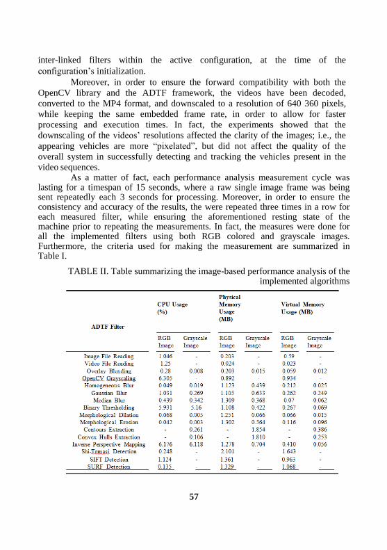
57
×
inter-linked filters within the active configuration, at the time of the
configuration’s initialization.
Moreover, in order to ensure the forward compatibility with both the
OpenCV library and the ADTF framework, the videos have been decoded,
converted to the MP4 format, and downscaled to a resolution of 640 360 pixels,
while keeping the same embedded frame rate, in order to allow for faster
processing and execution times. In fact, the experiments showed that the
downscaling of the videos’ resolutions affected the clarity of the images; i.e., the
appearing vehicles are more “pixelated”, but did not affect the quality of the
overall system in successfully detecting and tracking the vehicles present in the
video sequences. As a matter of fact, each performance analysis measurement cycle was
lasting for a timespan of 15 seconds, where a raw single image frame was being sent repeatedly each 3 seconds for processing. Moreover, in order to ensure the consistency and accuracy of the results, the were repeated three times in a row for each measured filter, while ensuring the aforementioned resting state of the machine prior to repeating the measurements. In fact, the measures were done for all the implemented filters using both RGB colored and grayscale images. Furthermore, the criteria used for making the measurement are summarized in Table I.
TABLE II. Table summarizing the image-based performance analysis of the implemented algorithms

58
The observed measurements for the Image File Reader and the Video File
Reader filters were deduced from the results of the measurements observed for
each analyzed filter, in order to alleviate the overhead caused by the extraction of
the image frames. In addition, the overhead caused by the Performance Analysis
filter has also been taken into account. The results of the analysis are summarized
in Table II.
As previously mentioned, the measures were done on single colored and
grayscaled image frames, and the values given by Table II represent the average
performance values of each respective implemented filter, except for the three
detection filters2. In fact, the image and video reading filters that were used to
extract the RGB colored image frames consumed relatively low physical and
virtual memory. Note that the colored RGB image frames were converted to their
grayscale equivalents using different grayscale conversion techniques, and that the
Single Color Channel conversion filter consumed the least amount of CPU usage,
whereas the algorithm behind the OpenCV grayscale conversion function
consumed the highest amount of memory, as depicted by Figure 4.
Moreover, the homogeneous blurring algorithm was observed to be the
most performant amongst all, which is in fact due to its simplicity of equally
weighting the images’ pixel intensities.
Fig. 4 - Figure showing the performance analysis of the grayscale
conversion filters in ADTF
Furthermore, it has been noticed that the binary thresholding using the
OpenCV functions requested more CPU usage than most of the other analyzed
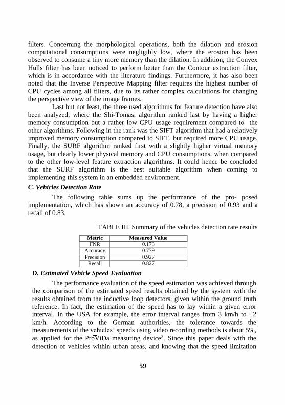
59
−
filters. Concerning the morphological operations, both the dilation and erosion
computational consumptions were negligibly low, where the erosion has been
observed to consume a tiny more memory than the dilation. In addition, the Convex
Hulls filter has been noticed to perform better than the Contour extraction filter,
which is in accordance with the literature findings. Furthermore, it has also been
noted that the Inverse Perspective Mapping filter requires the highest number of
CPU cycles among all filters, due to its rather complex calculations for changing
the perspective view of the image frames.
Last but not least, the three used algorithms for feature detection have also
been analyzed, where the Shi-Tomasi algorithm ranked last by having a higher
memory consumption but a rather low CPU usage requirement compared to the
other algorithms. Following in the rank was the SIFT algorithm that had a relatively
improved memory consumption compared to SIFT, but required more CPU usage.
Finally, the SURF algorithm ranked first with a slightly higher virtual memory
usage, but clearly lower physical memory and CPU consumptions, when compared
to the other low-level feature extraction algorithms. It could hence be concluded
that the SURF algorithm is the best suitable algorithm when coming to
implementing this system in an embedded environment.
C. Vehicles Detection Rate
The following table sums up the performance of the pro- posed
implementation, which has shown an accuracy of 0.78, a precision of 0.93 and a
recall of 0.83.
TABLE III. Summary of the vehicles detection rate results
Metric Measured Value
FNR 0.173
Accuracy 0.779
Precision 0.927
Recall 0.827
D. Estimated Vehicle Speed Evaluation
The performance evaluation of the speed estimation was achieved through
the comparison of the estimated speed results obtained by the system with the
results obtained from the inductive loop detectors, given within the ground truth
reference. In fact, the estimation of the speed has to lay within a given error
interval. In the USA for example, the error interval ranges from 3 km/h to +2
km/h. According to the German authorities, the tolerance towards the
measurements of the vehicles’ speeds using video recording methods is about 5%,
as applied for the ProViDa measuring device3. Since this paper deals with the
detection of vehicles within urban areas, and knowing that the speed limitation

60
−
within cities is set to 50 km/h, a valid output speed estimate should be within a
range of 2.5 km/h. Thus, the adopted standard is the one following the German
enforcements, due to its more restrictive measures.
Furthermore, the minimal and maximal error values recorded by the
system for the used dataset are respectively -4.98 and +3.51 km/h, whereas the
average absolute error was 1.328 km/h, making 76.322 % of the measured values
fall within the German tolerance range. Moreover, the feature tracker; which was
set up to select the best 15 features, achieved satisfying results in tracking the
vehicles in the different frames. In fact, the feature tracker was able to correctly
track; on average, 90.556 % of the vehicles that appeared in the videos.
V.CONCLUSION AND OUTLOOK
The goal of this paper has been to use low-level feature- based image
processing algorithms, in combination with a tracking algorithm, in order to be able
to detect vehicles in an urban environment, and estimate their corresponding speeds.
The work done in solving the aforementioned task consists of a sequential
processing chain made of various low-level processing filters implemented within
the ADTF framework, three main low-level features extraction algorithms; i.e., Shi-
Tomasi, Scale Invariant Feature Transform (SIFT) and Speeded-Up Robust
Features (SURF), a tracking mechanism based on the Kanade-Lucas-Tomasi (KLT)
algorithm, and an according scene interpretation that utilizes the approach of the
Inverse Perspective Mapping (IPM).
Furthermore, although several other modern feature extraction algorithms
are available in the literature, the focus of this paper has been directed towards the
usage and analysis of three low-level feature extraction algorithms, namely Shi-
Tomasi, SIFT and SURF, which are considered as being part of the most widely
used algorithms within the image processing research field. The analysis yielded
to the results that the Shi-Tomasi algorithm ranked last by having a higher
memory consumption but rather low CPU usage requirements when compared to
the other algorithms, followed by the SIFT algorithm that had a relatively improved
memory consumption compared to SIFT, but required more CPU usage, and finally,
the SURF algorithm that ranked first and showed its suitability for an embedded
implementation with a slightly higher virtual memory usage, but clearly lower
physical memory and CPU consumptions, when compared to the other low-level
feature extraction algorithms.
Last but not least, future scopes for further improving the presented
system could be proposed. These may consist amongst others of applying data and
task parallelization approaches [4], [5] for a better embedded performance
suitability, in cases where the handling of a bigger resolution input feed is required.

61
Furthermore, enhancements of the model could also be achieved by utilizing other
techniques useful for solving and consolidating the solution to the problem given
by the task. An example would be the addition of the Kalman Filter (KF) that could
be used in conjunction with the implemented KLT tracker, in order to alleviate the
problems of the tracking misses, by using the predictions of the Kalman filter, and
hence improve the overall tracking of vehicles. Furthermore, a 3D pose of the
appearing vehicles could also be estimated using the POSIT technique, which
would allow the precise localization and encapsulation of the 3D bounding
dimensions of the appearing vehicles. This would in fact compensate the lack of the
vehicles’ heights knowledge, and could be used to further improve the estimation
of the vehicles’ speeds.
Not to mention that since the implemented system’s soft- ware
components comply with the MISRA C++ rules, a possible embedded
implementation could be envisaged within the YellowCar project [6] undertaken at
the Computer Engineering Department of the Computer Science Faculty of the
Chemnitz University of Technology. The YellowCar’s ability to deal with
automotive real-time scenarios could eventually be enhanced by integrating the
proposed system into one of its existent ECUs.
REFERENCES
[1] The European Commission, Directorate-General Mobility and Transport, Unit C2 - Road Safety, “Road Safety in the European Union - Trends, statistics and main challenges,” European Commission, Tech. Rep., April 2018.
[2] Elektrobit Assist, “ADTF v2.13.1 SDK Documentation,” Audi Electronics Venture GmbH, Tech. Rep., July 2015.
[3] D. C. Luvizon, B. T. Nassu, and R. Minetto, “A Video-Based System for Vehicle Speed Measurement in Urban Roadways,” in IEEE Transactions on Intelligent Transportation Systems (ITS), September 2016, pp. 1–12.
[4] S. Blokzyl, M. Vodel, and W. Hardt, “A Hardware-accelerated Real-time Image Processing Concept for High-resolution Electro-optical Sensors,” Deutscher Luft- und Raumfahrtkongress, 2012.
[5] S. Blokzyl, M. Vodel, and W. Hardt, “FPGA-based Approach for Runway Boundary Detection in High-resolution Colour Images,” in Proceedings of the Sensors and Applications Symposium, 2014.
[6] N.Englisch, O. Khan, R. Mittag, F. Hanchen, W. Hardt, and A. Heller, “YellowCar: Automotive Multi-ECU Demonstrator Platform,” in IN- FORMATIK 2017, 15. GI Workshop Automotive Software Engineering, ser. Lecture Notes in Informatics (LNI) - Proceedings, Volume P-275, September 2017, pp. 1517–1522.

62
Face Recognition via Joint Feature Extraction based on
Multi-task Learning
Ao Li1, Deyun Chen
2, Guanglu Sun
3, Kezheng Lin
4
1,2,3,4Harbin University of Science and Technology (HUST)
[email protected] 1, [email protected]
2,
[email protected] 3, [email protected]
4
Abstract—In this paper, we proposed a novel joint feature extraction
framework to address the face recognition problem. It is found that different
face images have some hidden shared information, which can be used to help
to improve the recognition performance. Hence, the proposed framework take
face images for each person as a task, and then explored the shared and class-
specific structures across different persons simultaneously based on multi-task
learning. Meanwhile, an extra subspace projection for each person is also
learned to enhance the discrimination. Extensive experimental results
demonstrate that our proposed framework is superior among the existing face
recognition methods.
Keywords—Face recognition; Feature extraction; Multi-task learning;
I.INTRODUCTION
Face recognition is a fundamental issue in computer vision, which aims to
assign a query face into an known person in the database. Many literatures
aboutface recognition are emerged in the past two decades, and several recognition
frameworks are formed to address the face recognition problem. J. Wright et al
proposed a general classification method for robust face recognition with sparse
representation(SRC)[1]. In their method, the query sample was approximated by the
linear combination of training samples, and the label for face can be easily assigned
with a minimum class-specific local fidelity term. Then, to explore the intrinsic
character of SRC, the working mechanism of SRC is discussed in [2], and the
collaborative representation-based face recognition is proposed to reveal theory of
face recognition problem. A.. Wagner t al found that the face alignment can
significantly improve the recognition rate, and put the face alignment and classifier
into a unified framework to extend the conventional SRC model[3]. Q.Shi et al
analyze the face recognition from the view of sparsity, and talk about its relevant to
compressive sensing problem[4]. With the help of robust regression, M. Yang et al

63
proposed a robust regression coding method, and obtain excellent results in face
recognition issue[5]. Some more relevant literatures can be studied in [6-11].
Though the above linear regression-based methods achieved remarkable
performance to promote the accuracy recognition rate, they all utilized the training
face sample individually. Nevertheless, in practice, face images from different
persons have hidden shared features. If these shared features can be well studied, it
will improve the recognition performance greatly. Meanwhile, with the successful
application in mining shared information, multitask learning-based classification
model shows increasing interest in recent computer vision community. So, in this
paper, we introduced the multitask learning into the conventional model, and
established a joint feature extraction framework to address the face recognition
problem. To obtain extra discrimination, a discriminative projection is also learned
in our proposed framework. Experiments are tested on several face datasets to
verify the effectiveness.
The remainder of this paper is listed as follows. The detail of our proposed
model is discussed in Section II. Some experimental results are shown in Section
III. Section IV concludes the paper.
II. JOINT FEATURE EXTRACTION FRAMEWORK
A. Joint feature extraction model
For clarity, we first list some notations used in our paper. The training data
set is denoted as C
iiX1
, where iNd
i RX
presents training subset of i -th class
with iN instances , and d denotes the instance dimensionality. For each training
instance d
k Rx , let C
k Ry be its label vector, where C denotes the total
number of classes in the training set. Furthermore, if kx is chosen from the c -th
class( Cc ...3,2,1 ), only the c -th entry of ky is one and all others are zero. That
is, if kx is chosen from the second class, its label ky is denoted as
T
ky ,...]0,1,0[ . Let dCRW be the regression parameters as
TT
C
TT wwwW ,.., 21 , where each cw denotes the regression vector for c -th
class and can be seen as the classifier for the c -th class in regression-based
classification problem. With these notations, the general training model for W with
linear regression can be formulated as follows.
WWXYFW
2
min (1)

64
where ,...,..., 21 kyyyY denotes the label matrix for all the instances
( CXXXX ,.., 21 ) in training data set, W presents the certain constraint
on the parameters, F
denotes the Frobinus norm and is the positive scalar to
balance the two terms.
By enforcing the training data close to their labels, equation (3,1) aims to learn
the regression parameters from a mount of instances statistically. And then, the
label vector qy of a test instance
qx can be predicted with the parameters as
ˆˆq qy Wx , and the label ˆqc can be decided with ˆ ˆarg maxq q
c
c y c .
Similar to equation (1), what we want is to introduce the multitask learning to
our proposed model. In our model, we take face samples of each person as a task,
and explore the shared and class-specific structural components simultaneously
across different person, which is believed to help to extract extra joint information
hidden in different person to make the feature more effective. Based on this idea,
we formulated our proposed model as follows.
2
2
, ,1
1
mini i S
Ci S i i i F
S FW P Wi
i i
Q X W W PXW
P W
(2)
where iQ X is a designed operator to extract the Gabor feature, which is
used to transform the data matrix iX to a low-dimensional vector with respect to
its columns. SW and
iW denote the parameters to explore the shared structural
component among the tasks, and the class-specific structural component
respectively. iP represents the discriminative projection matrix for i th person.
, and are the positive constant to balance the terms in model. With our
proposed model in equation (2), shared and class-specific feature extraction
parameters, and discriminative subspace projections are learned simultaneously in a
unified framework. The three variables will benefit each other during the iteration,
which will improve the recognition performance progressively.
B.Numerical scheme for proposed model
Now, we will present a numerical scheme to solve the objective function in
the proposed model. The alternating direction method of multipliers(ADMM) has

65
been widely used in the multivariable minimization problems[12]. With ADMM,
our proposed model can be divided into three subproblems as follows, which can be
solved independently and iteratively.
For each task, fix its projection operator iP and class-specific structural
feature extraction parameter matrix iW , we can obtain the following subproblem for
SW .
2 2
, ,1
mini i S
C
i S i i i S FFW P Wi
Q X W W PX W
(3)
From equation (3), it can be seen that objective function is a convex and
differentiable function. By forcing its derivative to be zero, the closed- form
solution can be obtained in the k -th iteration as
1
1
1 1
C Ck T T
S i i i i i i s
i i
W Q X W I
(4)
where, i i iPX . T and 1 denote the transpose and inverse
operation on matrix. I presents the identity matrix.
Fixing the iP and SW , the class-specific structural feature extraction
parameters iW can be optimized by the minimization as follows.
2
1min
ii S i i i iFW
Q X W W PX W (5)
The objective function in (5) is a classical lasso problem, which can be
solved with the method in [13].
When the shared and class-specific feature extraction parameters are fixed,
we can obtain the minimization problem for projection operator iP as
2
2min
ii S i i i iFP
Q X W W PX P (6)
Similarly, forcing the objective function in (6) to be zero, we can easily
learn the projection operator. Based on the above equations, the numerical scheme for the proposed
model can be summarized as follows:

66
Numerical Algorithm
Initialization: Shared structural parameters 0
SW ,
class-specific structural parameters 0
iW and
projection operator 0
iP . Iterative step 0k .
While not converged do
1.Compute the shared parameters 1k
SW with
equation (3);
2. For i =1:C
(1) Compute the class-specific structural parameters
1k
iW with equation (5);
(2) Compute the projection operator structural
parameters iP with equation (5);
end for
End while
Output the parameters *
SW ,*
iW ,*
iP ;
with the learned parameters
SW , Ciii PW
1,
, a query sample qx can be
classified into a category by the self-regression loss term in our framework as
follows.
ˆ arg minq q S i i qFi
l Q x W W Px (3.19)
where ˆql denotes the estimated label indicator.

67
III. EXPERIMENTAL RESULTS AND ANALYSIS
In this section, we will conduct extensive experiments on several face
datasets. The proposed framework will be compared to existing excellent methods to
evaluate the competitive performance. In our experiments, the extended YaleB and
ORL face datasets are used test the performance. The comparison method includes
SRC, CRC and symmetrical face feature(SFF) proposed in []. The details of dataset
are described as follows.
The Extended YaleB face dataset contains a total of 16128 face images,
which were shot by 38 people under different lighting conditions. Each person has
64 positive face images under different expressions and lighting conditions. Fig.1
shows a small sample of the images in the data set.
Fig.1 instances of two persons in Extended YaleB
The ORL face dataset contains 400 face images, which were shot by 10
people under different lighting conditions, varying view and expressions. Each
person has about 10 face images. Figure 2 shows some face samples of the ORL
dataset.
Fig.2 instances of two persons in ORL
We performed simulation experiments on the above two face datasets
methods with the comparison methods. We test five time for each method, and take
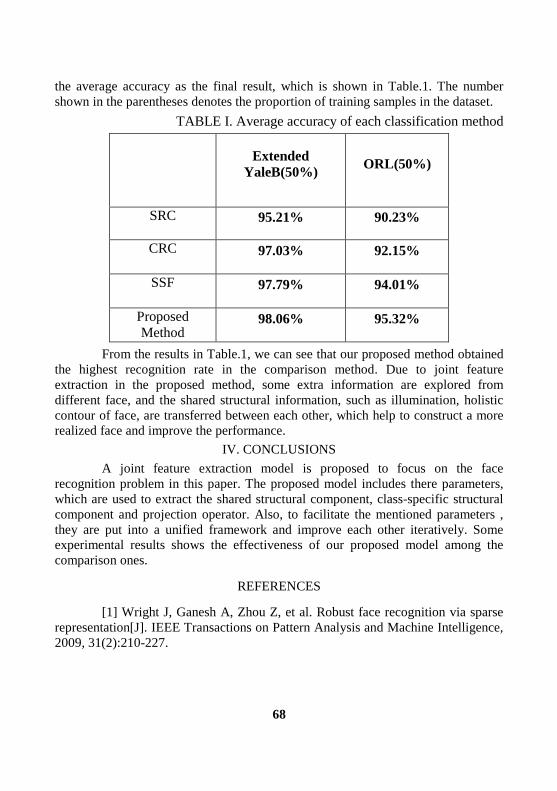
68
the average accuracy as the final result, which is shown in Table.1. The number
shown in the parentheses denotes the proportion of training samples in the dataset.
TABLE I. Average accuracy of each classification method
Extended
YaleB(50%) ORL(50%)
SRC 95.21% 90.23%
CRC 97.03% 92.15%
SSF 97.79% 94.01%
Proposed
Method 98.06% 95.32%
From the results in Table.1, we can see that our proposed method obtained
the highest recognition rate in the comparison method. Due to joint feature
extraction in the proposed method, some extra information are explored from
different face, and the shared structural information, such as illumination, holistic
contour of face, are transferred between each other, which help to construct a more
realized face and improve the performance.
IV. CONCLUSIONS
A joint feature extraction model is proposed to focus on the face
recognition problem in this paper. The proposed model includes there parameters,
which are used to extract the shared structural component, class-specific structural
component and projection operator. Also, to facilitate the mentioned parameters ,
they are put into a unified framework and improve each other iteratively. Some
experimental results shows the effectiveness of our proposed model among the
comparison ones.
REFERENCES
[1] Wright J, Ganesh A, Zhou Z, et al. Robust face recognition via sparse
representation[J]. IEEE Transactions on Pattern Analysis and Machine Intelligence,
2009, 31(2):210-227.

69
[2] Zhang L, Yang M, Feng XC. Sparse Representation or Collaborative
Representation: Which Helps Face Recognition?.[C] IEEE International Conference
on Computer Vision, 2011, Barcelona Spain, pp.471-478.
[3] Wagner, J. Wright, A. Ganesh, Z. H. Zhou, H. Mobahi, and Y.Ma,
“Toward a practical face recognition system: Robust registration and illumination
via sparse representation,” IEEE Trans. Pattern Anal. Mach. Intell., vol. 34, no. 2,
pp. 372–386, Feb. 2011
[4] Q. Shi, A. Eriksson, A. Hengel, and C. Shen, “Is face recognition
[5] M. Yang, L. Zhang, J. Yang, and D. Zhang, “Regularized robust coding
for face recognition,” IEEE Trans. Image Process., vol. 22, no. 5, pp. 1753–1766,
May 2013.
[6] R. He, W. S. Zheng, B. G. Hu, and X. W. Kong, “A regularized
correntropy framework for robust pattern recognition,” Neural Comput.,
vol. 23, pp. 2074–2100, 2011.
[7] R. He, W. S. Zheng, and B. G. Hu, “Maximum correntropy criterion for
robust face recognition,” IEEE Trans. Pattern Anal. Mach. Intell., vol. 33, no. 8, pp.
1561–1576, Aug. 2011.
[8] X.-X. Li, D.-Q. Dai, X.-F. Zhang, and C.-X. Ren, “Structured sparse
error coding for face recognition with occlusion,” IEEE Trans. Image Process., vol.
22 , no. 5, pp. 1889–1999, May 2013.
[9] R. Rigamonti, M. Brown, and V. Lepetit, “Are sparse representations
really relevant for image classification?” in Proc. IEEE Conf. Comput. Vis. Pattern
Recog., 2011, pp. 1545–1552.
[10]I. Naseem, R. Togneri, and M. Bennamoun, “Robust regression for
face recognition,” Pattern Recog., vol. 45, pp. 104–118, 2012.
[11] A.M. Martinez, Recognizing imprecisely localized, partially occluded,
and expression variant faces from a single sample per class, IEEE Transactions on
Pattern Analysis and Machine Intelligence 25 (6) (2002) 748–763.
[12] S. Boyd, N. Parikh, E. Chu, B. Peleato, and J. Eckstein, “Distributed
optimization and statistical learning via the alternating direction method of
multipliers,” Found. Trends Mach. Learn.,vol. 3, no. 1, p. 1122, 2011.
[13] P. Zhao and B. Yu, “On Model Selection Consistency of Lasso,” J.
Machine Learning Research, no. 7, pp. 2541-2567, 2006.
[14] Y.Xu, X.Z Zhu, Z.M Li, et al. Using the original and ‘symmetrical
face’ training samples to perform representation based two-step face recognition.[J]
Pattern Recognition, 46:1151-1158,2013.

70
Automated setting Eye Diagram for optimization of
optical transceiver manufacturing process
Mikhail E. Pazhetnov
Novosibirsk State Technical University (NSTU)
Abstract - This article describes how to set up optical transceivers
using the Eye Diagram. Uncover the essence of one of the methods for
optimizing the production of optical transceivers. The program part, methods
used to implement automated configuration, are described. The basic
principles of the Eye Diagrams applying to evaluate the correct data transfer
in the optical transceiver are shown.
Keywords - Eye diagram, optical transceiver, FOCL, automated setting.
I. INTRODUCTION
At the current stage of modern society development and modern means of
communication, it is impossible to overestimate the growth and development of the
Internet technologies. Where there's demand, there's supply. Because of that the
various communication lines are rapidly developing and researched, which must
meet future requests for data transmission capacity. One of these methods is fiber-
optic technology.
Fiber-optic technology implies a way of transmitting information in which
electromagnetic radiation of the optical (near infrared) range is used as the
information signal carrier, and cables made of optical fiber serve as guide systems.
FOCL has several advantages. Mainly, the fiber optic link has a high
transfer rate and a sufficiently high protection against noise, due to the fact that the
fiber is made of a dielectric material. Also, a very significant advantage is the
security of data transmission. The fact, is that the cable has practically no radio
emission, creating an unfavorable environment for attackers, for theft of transmitted
data. Unlike a copper cable, to obtain the transmitted information, without
penetrating into the channel, is much more labor-intensive. A monitoring system
allows you to notify and stop attempts to "hack" the channel. In this regard, the
technology of the fiber optic communication line is actively used wherever a secure
transmission of data is required.
When using fiber optic technology and organizing an optical connection,
optical transceivers. They appear as an electron-optical converter. The technology

71
of manufacturing optical transceivers is quite complicated. It consists of a large
number of stages that follow one another. And, the final result is affected by the
success of each of them. Therefore, there is an urgent issue of optimizing the
production of optical transceivers. Each enterprise, regardless of the product being
produced, aims at exploring those technological solutions that will increase
production rates, reduce the amount of waste and costs. As the proposed method,
consider the automation of the process of setting up the correct data transfer. It is
based on the construction of the Eye Diagram.
II. THE EYE DIAGRAM
The Eye Diagram is a graphical method for evaluating the quality of a
digital output electrical signal, which is the sum of all the bit periods of the
measured signal superimposed on each other. It is the result of superimposing all
possible pulse sequences over a period of time equal to two clock intervals of the
linear signal. With its help, you can understand at what level of accuracy data is
transmitted over the communication channel. The use of the Eye Diagram is
considered to be a rough but fast method of obtaining a sufficiently good estimate
of the quality of the received signal.
To confirm the fact of qualitative data transfer, it is analyzed: opening of
the eyes (distance from the upper to the lower boundary), average power
(intersection), signal-to-noise ratio, mask margin, upper and lower boundaries of
the diagram. When analyzing the mask margin, the following approach is used: if
the signal lines on the display remain outside the mask boundaries, then the scheme
is considered of acceptable quality. The height from the top to the bottom of the
Eye Diagram is a measure of noise in signal. As soon as the lines become thicker
and shorter, the circuit turns out to be more susceptible to noise and the signal
quality can be expected to deteriorate. The width of the signal in the central part of
the Eye Diagram is a measure of the accumulated jitter (phase jitter). If the lines are
thin then the level of accumulated jitter is small. The wider the line in the center of
the Eye Diagram, the greater the jitter level.
The process of analyzing the correct Eye Diagram can be automated. In
order to influence the oscilloscope chart, in the optical transceiver itself, the bias,
modulation and phase shift readings are changed, which in turn are written in the
form of byte sequences. There is a huge number of processors on which optical
transceivers are built. Correspondingly each type has its own algorithm for storing
and initialize the service information.

72
Fig. 1 – Normal Eye diagram
Fig. 2 – Eye Diagram with high level jitter and without mask margin.

73
III. AUTOMATED SETTINGS OF THE EYE DIAGRAM
The system can be represented as follows: a ready-to-configure optical
transceiver is installed in the debug board. The debug board is attached to the
oscilloscope, the bit error generator, and to the computer. The developed software
part combines:
1) Oscilloscope management.
In the program window, you can configure the oscilloscope operation
modes, the frequency of updating the indications, the number of points participating
in the drawing of the diagram, and so on.
2) Visual display of the Eye Diagram.
In a separate window, an oscillogram is displayed in the form of a cluster
of small dots. The display itself is necessary for visual analysis of the diagram in
the case of manual tuning. In addition, the necessary parameters are duplicated in
the TextBox. This whole complex helps to prevent accidental program errors.
3) Interface for connecting and setting up the optical transceiver.
Here are the sliders for the visual change of values in the optical
transceiver. When the module is initialized on the debug board, the program reads
the readings itself, sets the acceptable threshold values and visually displays the
Bias and modulation values in the Textbox.
4) Interface of automated mode of eye chart adjustment
To start the automated mode, you only need to enter the desired indications
for opening the eye and the level of intersection. By pressing the "Auto" button, the
system will start selecting the necessary parameters, which can be observed in the
settings panel. Also, to increase the speed of automated setting, the function of
changing the error was added. As the error increases, the tuning time increases.
With its decrease, the set parameters approach the desired values as much as
possible, but the adjustment takes longer.
Adjustment mechanism
In order to use automated setting, enough optimization methods have been
considered, such as: PI regulator, PID regulator and so on, but in the course of
studying these methods, it was revealed that in order to calculate and predict the
necessary parameters for a correct Eye Diagram, it takes time, and also it was not
exact but close to the linear dependence of the bios on the level of intersection and
modulation to the level of opening of the eye. The most optimal tuning algorithm
was the method of binary segments (Bisection method). Firstly, it is easy enough to
perform. Secondly, the required speed of adjustment was obtained. Thirdly, almost
every optical transceiver, even with the same components, shows a different picture
of the Eye Diagrams during the tuning phase, therefore it will not be possible to
calculate the coefficients and a priori to specify the parameters.

74
With reference to this problem, the classical method of bisection looks like
this:
Provided that the current value is greater than required:
BL = currentvalue; (1)
X = (RB - currentvalue) / 2 (2)
Provided that the current value is less than required:
BR = currentvalue; (3)
X = (BL - currentvalue) / 2 (4)
Where X is the value:
BL - Left border.
BR - Right border.
The condition for the completion of the algorithm is the comparison of the
error and the difference between the actual and the required value.
Error estimation> = | Actual - Required | (5)
IV. EXPERIMENT AND RESULTS
As an experiment, the manual and automated adjustment of eye diagrams
was tested. 100 pieces of optical transceivers were selected, 50 of which were
manually tuned and 50 were in automated mode. During the experiment it was
found, that in manual mode the test time was 45 minutes, and in automated mode,
31 minutes. As a result, productivity increased 1.45 times. This is a significant
result, given the production volumes. In addition, automated mode implies only
control by the operator, excluding the human factor (tiredness, inattention). The
operator just needs to set the correct type of optical transceiver and watch the Eye
Diagram change. In the end of the testing phase, the program recalls it with a pop-
up window.
Fig. 3 – Optical transceiver initialization

75
Fig. 4 – Customized Optical transceiver
V. CONCLUSION
Throughout the World, including in Russian Federation, the demand for
fiber-optic communication is only increasing. In this connection, the further
prospect of development of FOCL technologies in information networks is obvious.
Of course, there is a need for research and development of solutions in this area.
Accordingly, the topicality of the development of optical systems investigations
arises from this.
In order to increase the performance of optical transceivers, the task was to
automatize the adjustment of the optical eye. In the course of development, the shell
for the oscilloscope API was written and the interface for the initialization and
setup of optical transceivers was fully developed. The software part is developed
taking into account the addition of new types of optical transceivers and auxiliary
devices. In the future, the system will be tested in a longer mode, at the end of
which, a verdict will be approved about further refinement or start-up of the system.
REFERENCES
[1] Harbour, Stephen. Soliton Research May Improve Optical Fiber
Transmission. – "EuroPhotonics", Oct/Nov, 1998, p. 38-39.
[2] Nakazawa, Masataka. Telecommunications Rides a New Wave. –
Photonics Spectra. Feb. 2016, p. 97 104.
[3] Eye diagram analysis. 21.10.2018. / [Electronic resource]. -
http://www.mathworks.com/ - Title from screen.

76
Experience In Implementing Project Training In A
Technical University
Alexander.A. Yakimenko
Novosibirsk State Technical University (NSTU)
Abstract - The object of research was the technology of project-oriented learning. The aim of the research was to study the experience of project training and evaluate the possibility of introducing technologies of project-oriented learning in the educational process of the NSTU. In conclusion, the features of the organization of project activities in the university are given.
Keywords - project training, practice-oriented training, project method,
team work
I. INTRODUCTION
Education systems are called upon to contribute to the realization of the
main tasks of the socioeconomic and cultural development of society, for it is the
school and the university that prepare the person for active work in various spheres
of the economy, culture, and political life of society.
The analysis showed that the problematic situation of modern education is
that the teaching technologies have changed little over the past two hundred years.
In essence, the teacher of the modern university does the same thing as the
university professor of the 19th century: for example, Herbart, who offered a class-
lesson system and a specific lesson plan for the lesson.
The Information Society is interested in ensuring that its citizens are able to
act independently, take decisions, adapt flexibly to the changing conditions of life:
- Flexibly adapt in changing life situations, independently acquire the
necessary knowledge, skillfully applying them in practice to solve a variety of
emerging problems, so that throughout life you can find a place in it;
- independently think critically, be able to see the problems arising in real
life and seek ways to rationally solve them using modern technologies; clearly
understand where and how the knowledge they acquire can be applied in their
environment; be able to generate new ideas, think creatively;
- Competently to work with information (be able to collect the facts
necessary for solving a certain problem, analyze them, put forward hypotheses for
solving problems, make necessary generalizations, compare them with similar or

77
alternative solutions, establish statistical regularities, draw reasoned conclusions,
apply the findings to identify and solve new problems);
- be communicative, contact in various social groups, be able to work
together in various fields, in different situations, preventing or skillfully leaving any
conflict situations;
- independently work on the development of their own morality, intellect,
cultural level.
The above requirements are implemented in the global pedagogical
community in the framework of various programs and projects, including the
implementation of a competence approach.
II. ITRAINING IN COOPERATION
Training in small groups was used in pedagogy for a long time. It is an
important element of the pragmatic approach to education in the philosophy of J.
Dewey, his project method, developed principles and methods of problem-based
learning [1]. According to him, these methods have undeniable advantages
compared to explanatory-illustrative. The problem situations created during the
educational process can reveal the inadequacy of the knowledge previously learned
by the students, which encourages them to search, promotes the formation of
cognitive independence, development of critical thinking and creative abilities.
A. Syndicate method
Provides that a large group of students (usually a whole course) is divided
into subgroups of 4-6 people. These groups work during the seminar, performing
certain collective tasks. After some time, the course is going together to discuss the
results of the subgroup work [2].
B. Grouping
The group can be divided into separate individual tasks. Group work can
take part of the seminar, the whole seminar or even several lessons in a row. Each
subgroup is then divided with the whole group by the results of its work. Unlike the
syndicate method, the main work unit here is the whole seminar group, the
subgroups are organized only if necessary. The function of the teacher is to
summarize, give necessary explanations, introduce and explain new tasks [3].
C. Division of lessons
The whole seminar group spends half the time with the teacher, half
without it. During the meetings with the teacher, the work the group has done on its
own is discussed, and the next self-study is planned.

78
D. Interconnections of participants in project training
In the described approaches, we can distinguish three types of
interdependence of participants in joint training:
1. Dependence on a single goal, which is realized by the students and
which they can achieve only through joint efforts.
2. Dependence on information sources, when each student of the group
owns only a part of the general information or a source of information that is
necessary to solve the overall task; everyone must contribute to the solution of the
common task. This dependence can be at the level of the division of labor, role
functions, training material (tools, equipment), divided between the students of the
group (for example, one scissors, one sheet of paper, one paint, etc.).
3. Dependence on the form of encouragement. Each student receives the
same grade for the work. Either all are encouraged the same way, or are not
encouraged in any way.
III. PROJECT TRAINING (PROJECT METHOD)
• The educational process is built not in the logic of the academic subject,
but in the logic of activity that has a personal meaning for the trainee, which
increases its motivation in the teaching;
• The solution of a specific problem of the surrounding reality is placed at
the center of the process of creating an educational project;
• The teacher is only the guiding link in the activity, the process of creating
the educational project is focused on the independent activity of the trainees;
• The trainee becomes the subject of the education process, sets goals and
selects information, determines its necessity, based on the design of its project;
• An integrated approach to the development of educational projects
promotes the development of general educational, communicative and research
skills;
• The individual pace of work on the educational project ensures the exit of
each student to their level of development;
• A deep, conscious assimilation of basic knowledge is ensured through the
universal use of them in different situations.
The purpose of project training is to create the conditions under which
students: 1) independently acquire new knowledge from different sources; 2) learn
to use the acquired knowledge to solve cognitive and practical problems; 3) acquire
communication skills, working in groups; 4) develop their research skills (the
ability to identify problems, collect information, observe, conduct experiments,
analyze, construct hypotheses, generalize, etc.) and system thinking.

79
At the heart of the project method is the development of cognitive skills of
students, the ability to independently design their knowledge, skills to navigate in
the information space, the development of critical thinking.
The method of projects is always focused on the independent activity of
students - individual, pair, group, which students perform for a certain period of
time. This approach is organically combined with a cooperative learning approach
to learning. The method of projects always involves the solution of a problem that
involves, on the one hand, the use of various methods and means of instruction, and
on the other, the integration of knowledge and skills from various fields of science,
technology, technology, and creative fields. The results of the completed projects
should be, as they say, "tangible," ie, if this is a theoretical problem, then its
concrete solution, if practical, concrete result, ready for implementation [4].
IV. BASIC REQUIREMENTS FOR USING THE PROJECT METHOD
1. The existence of a significant / research / creative problem / problem
requiring an integrated knowledge, research search for its solution.
2. Practical, theoretical, cognitive significance of the expected results (for
example, a report, a joint article, product registration or patenting ... etc.)
3. Independent (individual, pair, group) activities of students.
4. Structuring the substantive part of the project (indicating step-by-step
results).
Use of research methods:
• the definition of the problem, the research problems arising from it,
• the hypothesis of their solution,
• discussion of research methods,
• formalization of the final results,
• analysis of the data obtained,
•summarizing,
• adjustment,
• Conclusions (use of the method of "brainstorm", "round table", statistical
methods, creative reports, views, etc.).
Experience shows that joint projects based on cooperation between
students from different faculties, universities, cities and countries are most
effective.

80
TA
BL
E I
. S
tag
es o
f p
roje
ct a
ctiv
itie
s an
d t
he
inte
ract
ion
of
the
teac
her
an
d s
tud
ent
on t
hem
[5]
Acti
vit
y o
f th
e s
tud
en
t
Dis
cuss
ion
of
the
sub
ject
of
the
stu
dy a
nd
ob
tain
ing a
dd
itio
nal
info
rmat
ion i
f n
eces
sary
, se
ttin
g
rese
arch
ob
ject
ives
Fo
rmu
lati
on o
f re
sear
ch t
asks,
iden
tifi
cati
on
of
info
rmat
ion
sou
rces
Dra
win
g u
p a
n a
ctio
n p
lan,
info
rmat
ion g
ath
eri
ng
, p
ract
ical
imp
lem
enta
tio
n o
f se
lect
ed r
ole
s,
exec
uti
on
of
rele
van
t fu
nct
ions
An
aly
sis
of
the
info
rmat
ion
rece
ived
, a
com
bin
atio
n o
f id
eas,
thei
r g
ener
aliz
atio
n,
the
pro
mo
tio
n o
f a
com
mo
n i
dea
Pu
bli
c p
rote
ctio
n o
f th
e
edu
cati
on
al p
roje
ct
Ref
lect
ion
of
the
pro
ject
imp
lem
enta
tio
n p
roce
ss,
self
-
asse
ssm
ent
in t
he
fram
ework
of
the
pro
ject
act
ivit
y,
pro
mp
tin
g t
o
acq
uir
e n
ew k
no
wle
dg
e
Th
e a
cti
vit
y o
f th
e t
ea
ch
er
Det
erm
inat
ion
of
the
sub
ject
of
rese
arch
, m
oti
vat
ion
of
edu
cati
on
al a
nd
pro
fess
ion
al a
ctiv
itie
s, a
ssis
tan
ce
in s
etti
ng
th
e g
oal
s o
f th
e tr
ain
ing
pro
ject
Sta
tem
ents
ab
ou
t th
e ch
oic
e o
f so
urc
es,
way
s o
f
coll
ecti
ng
an
d a
nal
yzi
ng
in
form
atio
n,
corr
ect
ion
of
task
s as
sig
ned
to
tra
inee
s, d
efin
itio
n o
f ro
les
in
acco
rdan
ce w
ith t
he
sele
cted
co
mp
on
ents
of
the
init
ial
pro
ble
m
Su
bm
issi
on
of
spec
iall
y s
elec
ted
mat
eria
ls t
o e
ach
par
tici
pan
t o
f th
e p
roje
ct,
con
sult
atio
ns,
co
ord
inat
ion
of
the
trai
nee
s' w
ork
, m
on
ito
rin
g o
f th
e p
rog
ress
of
the
per
form
ed w
ork
, m
oti
vat
ion
fo
r an
d s
tim
ula
tio
n
of
acti
vit
ies
thro
ug
h r
ewar
ds
Iden
tifi
cati
on
of
sho
rtco
min
gs,
pro
vis
ion o
f ad
vic
e o
n
thei
r el
imin
atio
n,
con
sult
ing o
n p
rep
arat
ion
of
acco
mp
any
ing
pro
ject
do
cum
enta
tio
n
Org
aniz
atio
n o
f ex
per
tise
Sy
nth
esis
of
rev
iew
s an
d f
eed
bac
k f
rom
th
e e
xp
ert
com
mis
sio
n,
a p
rog
no
stic
ass
essm
ent
of
the
org
aniz
atio
n o
f th
e im
ple
men
tati
on p
roce
ss
Th
e t
ask
s of
the s
tage
Def
init
ion
of
obje
ctiv
es,
sele
ctio
n o
f
work
ing
gro
ups
Anal
ysi
s of
the
pro
ble
m,
iden
tifi
cati
on
of
sourc
es o
f in
form
atio
n,
stat
emen
t of
task
s, d
istr
ibuti
on
of
role
s in
the
team
Solv
ing
indiv
idual
pro
ble
ms
Anal
ysi
s of
the
deg
ree
of
achie
vem
ent
of
each
tas
k,
coll
ecti
on,
des
ign o
f th
e
pro
ject
Pre
senta
tion
of
the
educa
tional
pro
ject
Eval
uat
ion
of
the
resu
lts
of
the
trai
nin
g
pro
ject
and
the
pro
cess
of
its
imple
men
tati
on
Th
e s
tag
e o
f th
e
pro
ject
acti
vit
y
1.
Th
e T
ru
st
2.
An
aly
tica
l
3.
Rese
arch
4.
Co
nst
ru
cti
on
al
5.
Prese
nta
tio
n
6.
Refl
ecti
ve-
ev
alu
ati
ve

81
V. LIMITATIONS ON THE USE OF THE PROJECT TRAINING
The project method has its limitations, which must be taken into account
when planning its activities in the technology of project-oriented learning:
• low motivation of students to participate in the project;
• Inadequate level of formation in the students of research skills;
• impossibility to acquire professional and training skills in the course of
project activities;
• The difficulty in determining the criteria for evaluating the results of the
project activity.
VI. CONCLUSIONS
One of the main features of modern educational programs in the areas of
engineering education is the need to develop decision-making skills, their rationale
and ensure organizational and instrumental support. This is due at least to two
factors. First, most engineers sooner or later become managers (linear, middle or
senior) and, consequently, are forced to make managerial decisions, and secondly,
engineering itself involves the adoption of numerous technical and technological
solutions (designing the best engine design, choosing the optimal sequence
processing task flows and the optimal mode of operation of power plants and many
others).
The logic of modern innovative programs of engineering education
predetermines not only the inclusion of a block of courses related to effective
management (strategic and operational production management, project
management, innovative management, etc.), but also the use of active teaching
methods, including problem and project technologies learning.
Educational programs of engineering education are characterized by:
- a large number of laboratory works performed, as a rule, by groups of
students, which can be regarded as a prototype of the project,
- a large number of course projects and calculation and graphic works,
- the practical focus of most of the diploma projects being carried out,
- the presence of social partners - organizations interested in the results of
research and development projects of the technical university, in which students
take an active part,
- a significant "rejuvenation" of some engineering specialties, when there
is a situation in which the student often starts on the third year of the labor market
more in demand than his teachers [6].

82
REFERENCES
[1]. Beane W. E., Lemke E. A. Group variables influencing the transfer of
conceptual behavior // J. Educat. Psychol. 1971. V. 62(3). P. 215—218.
[2]. Hänsel D. Handbuch Projektunterricht. Weinheim 1997.
[3]. Hudgins B. Effects of group experience on individual problem solving
// J. Educat. Psychol. 1960. V. 51(1). P. 37—42.
[4]. Atanov G.A. Activity approach in training. - Donetsk: "EAI-press",
2001. - 160 with.
[5]. Gafurova N.V. Integral model of the intellectual-personal development
of students in the education system / Gafurova N. V .. - M .: MAKS Press, 2004.-
219 p.
[6]. Romanov E. L. Teaching software engineering. A look from the code
[Electronic resource] / EL Romanov, GV Troshina, AA Yakimenko // Science:
Internet magazine: electron. journal. - 2016. - Volume 8, No. 5. - Access mode:
http://naukovedenie.ru/PDF/66TVN516.pdf (access is free). Ver. from the screen. -
Ver. from the screen.

83
Challenges of learning analytics and the current
situation
Battsetseg Ts1, Munkhchimeg B
2, Bolor Lkh
3
1,2,3Mongolian University of Science and Technology (MUST)
[email protected] 1, [email protected]
2,
Abstract - An essential part of the activities of educational institutions
and universities is the selection and development of the learning management
system (LMS) thus there is created an experience in developing a variety of
methodologies to guide the research work collecting and processing of large
amounts of data and and reporting organizational data for decision making.
The learning management system data can not be very substantial for decision
making, concerned with processing data which is created in the learning
environment, evaluating the learning quality and contents, improving study
program. Evaluation of the learning system varies greatly depending on each
country's growth level, the characteristics of the educational system, and the
university's curriculum.
Keywords - learning analytics, learning management system data, data
mining, WEKA
I. INTRODUCTION
Since introducing of the learning management system in the university
activities, the biggest challenge that universities are facing is the immense and
quick growth of the educational data. In many research works were reflected on
implementation learning analytics such as to identify the factors which influence
the learning quality, to predicate students’ performance and analyse its impact
parameters, to evaluate study program, contents, quizzes, exams, and educator`s
activity through processing data.
Many universities around the world take into account different factors that
influence student`s learning performance, but it is not inadequate to make a
conclusion using commonly used factors.
It's proved that various factors such as previous learning background,
general admission score, governance, age, parents education level, where graduate
high school, major and GPA affect to students` learning performance and all of
these factors are used to predict students’ performance.

84
It is important to form log data of learning process or traceability for
collecting the necessary data evaluating learning activity. Factors, influencing to the
student`s learning performance have internal and external characteristics. It is
important to define students’ learning style and to create effective learning
environment by using suitable learning activities for reducing side effect of
unsuccessful learning such as drop out, students at risk. There has been used main
conclusion in around 600 researches in last 10 years to develop LMS, to process, to
mine learning environment data and to analyse learning factors.
II. RESEARCH PURPOSE
[1] To introduce research work Learning Analytics.
[2] To determine required data for development LMS which can provide
effective data to make decision, to improve university learning quality.
[3]To introduce learning analytics tool.
III. RELATED WORK
1. To determine appropriate method by comparing data mining methods
for processing learning environment data
2. To determine precision evaluation using methodology prediction
students learning performance
3. To analyse affecting learning factor
4. Research works of learning analytics, implementation experience of
learning analytics, research report of data processing gathered for long time of
period
5. Educational data mining, learning factor analyse, role of LMS for EDM,
mathematic model and theories of learning analytics are dominant research field for
USA researchers
Several core of problems was decided by research work on this field
during development of LMS are: usage of LMS function for learning activity, to
establish learning enviroment available online learning tools, to implement face to
face learning methodology in online learning environment, to accomplish flexible
learning such as collaboration, cooperative, interactivity, to built up most suitable
way to distribute learning content, to choice and use LMS optimally.
The selection of top learning management systems and introduce of results
contributes to the implementation and development of training systems educational
institutions and universities. However, the evaluation of the learning management
system varies greatly depending on the level of development, nationality, features
of education system, and university education policy.

85
IV. DATA ANALYSIS
In research works of learning analytics were used more than 50 factors
such as previous learning background, general admission score, demographic
details, social status etc and the impact parameters were different for each country.
A. Types of data
Large amounts of data are gathered in universities for helping improve the
learning quality and activities.
Table 1. illustrates the types of available data in the LMS. The first column
includes data that is regularly produced by LMS. The second column is an
illustration of the types of data that is provided by the educator that can be stored in
the LMS.
TABLE I. Types of data available for Learning analytics
Data generated by LMS Data generated by Instructor
Number of times spend Grades on exchange forum
Date and time of access Assignment marks
Number of discussion posts
generated
Grades on tests
Number of discussion posts read Final grades
Types of resource accessed Questions asked in discussion forum
E-mails notification ot/for instructor
attendance
B. Data attributes
The type of data is classified according to the field's properties. It is
basically divided into numerical (quantitative) and categorical (qualitative).
Numerical data has significance as numbers, and order, distance and equality of two
numerical variables. In opposition, categorical data has no meaning as figures only
correspondence within two definite variables.
Numeric data is organized as discrete or continuous. Discrete data
countably many values, and if the domain is portrayed on the number line, it

86
consists only of isolated cases. Discrete numbers are not always integers as it can be
decimal numbers with a predefined precision. The categorical variables can be
further classified as nominal or ordinal. The nominal values are only named for
sections and have no other meaning than classifying.The purpose of the research
work is to analyze the large unprocessed data generated in the learning environment
and to produce effective data.
Learning activity analysis is aimed to gather the data and analyse them.
Data mining is concerned with the implementation automation tools identifying of
big data trends which is created in learning process and developing its activity.
By implementing the theory and methodology of learning process analysis
educators and instructors process data creating in the learning environment and to
find more optimal decision, to manage learners successfully, to implement strategy
improving quality in this way can be created the free space to reach more efficient
result.
The important tool will be created to evaluate the learning process and to
make the decision by collecting and processing effective and qualitative data in
LMS. Therefore, within the framework of the research work, the type of data is
defined and by processing these data it can help to evaluate students` performance
and to identify factors affecting learning quality (Figure 1).
Fig. 1. Data types collecting in LMS
Learning activity analysis and data mining etc essential terms are very
common and differ in their use and study and research field. It is the theoretical
concept covering the machine learning, artificial intelligence, estimation methods,

87
recycling data and data visualization techniques. Research works is linked
inseparable with methodology data mining, smart system and personalized learning.
There is a growing need for data collection in education and the use of data
mining tools. This emerging trend is named as a data mining in the learning
environment (educational data mining) and is being developed as a research study
to use big data processing techniques. One of the main problem deciding by data
mining methods is to create the methodology predicting students’ performance.
Educational data mining consider on detecting algorithm of the data style
and developing new procedure. Data analysis of the learning environment consider
how to adopt above methodology in the learning activity.
It is considered that one of the ratio students’ performance and admission
operations is the success continue of learners.
The methodology of predicting students’ performance is detected
unsuccessful learning and it is important to develop a decision-making system to
improve the learning quality and data mining is used for this purpose.
V. PREPROCESSING OF DATA
There has compared and analysed in student assessments who has studied Mathematic, Physic and Information technology-1 in the Unimis learning system from 2014 to 2017.
1. The original data was 37044, therefrom after deleted 8177 data which is
concerned with 872 duplicated data for change profession or study dual profession,
1109 retrained data, 3538 Withdrawal (W), 2658 Exam incomplete by the student
(E) and 2658 Repeating a course (R) 28177 data left (Table 2).

88
TABLE II. Lesson evaluation data
Lesson Row
data
1 2 3 4 5 6 7
Total
(1-5)
NET
TOTAL Duplicated Retrained W E
no
pass
exam
R
passed
exam
R
F
U.IT101 7689 750 77 903 700 115 103 386 2545 5144
S.PH101 13000 122 510 1200 881 107 173 1272 2820 10180
S.MT101 16355 0 522 1435 1077 163 153 1457 3197 13158
2. After deleted all null data which is concerned with mathematics entrance
exam, teacher’s score, midterm exams etc 17674 data left (Table 3).
TABLE III. Percentage of adequate data
Fields U.IT101 S.PH101 S.MT101
UNIMIS row data 7689 13000 16355
Midterms, teacher score, exam score,
general admission score of mathematics 3591 6430 7653
Data persentage meet the requirements of
analysis
47% 49% 47%
3. There are not deleted null data from the Teacher code and Entrance
location. 4. It has done first step to analyse for learning evaluation that general
admission score, total score, exam score, teacher score, student code, student name,
school and profession etc (Figure 2).
Shown by chart which is distribution of students evaluation of
performanced students of selected lesson. In research work highlighted about it can
concluded that mentioned lessons have standard distribution. But it is impossible to
determine factors that evaluation affect, improvement and renewment for details list
of teacher’s score.
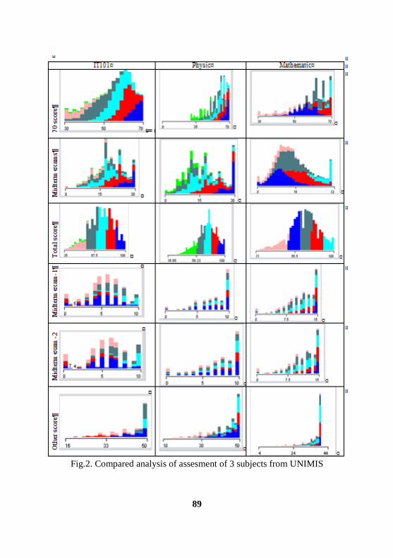
89
Fig.2. Compared analysis of assesment of 3 subjects from UNIMIS

90
V. WEKA TOOL
Weka is a graphical user interface tool that includes algorithms for data
analysis and predictive modeling, and data visualation methods. It is now used in
many different application areas, in particular for educational purposes and research.
Weka provides a number of methodologies of extraction of data, such as
preprocessing, classification, clustering, associations, and visualization.
There is shown students` assessments who has studied Information
technology-1 (Figure 3). In figure 1 was shown type of data generated by data
collecting and storing necessary for the decision making and here fewer data types
were selected and analyzed. It is a graphical way of preparing data to process the
Weka program.
Fig.3. Data visualation of student assesment for IT-1 last 4 years in Weka
VI. CONCLUSION
Analysing learning activity log data which is gathered by using various
type of learning content through LMS is making requirement to develop decision
support system. This type of data analysis helps to identify students 'learning styles
and develop a suitable training strategy to differentiate students' progress so that

91
flexibility can be followed by the fact that students in one group have different
levels of knowledge and skills.
Although the academic result analysis by final exam and course evaluation
curve is the first performance in UNIMIS (University Management Information
System) of Mongolian University of Science and Technology (MUST), different
methodology of teachers’ assessment negative impact on the end result of this work.
The following conclusions are being made from experimental work on the
disaggregated assessment of students' knowledge assessment.
1. The student`s duplicate data arise when the student changes his or her
profession or studies double major.
2. There is a need to monitor the accuracy and reality of the data collected
in the system. It was difficult to analyze data which entered into the field of data
teacher's score, two mid term exam scores (maximum score is 50 points) are
exceeding the limit.
3. 70/30 score analysis is not enough to assess the effectiveness of the
lesson, and it is important to decide the data type is inadequate to determine the
factors that influence the failure of the W evaluation analysis to do.
4. The differences in the methodology of academic affairs of the various
universities (MUST has 8 branch universities) are evident from the R values.
Therefore it is necessary to provide training for the employees of academic affairs.
5. There is a need to evaluate same methodology, to unify difference
teachers’ assessment of W.
6. Evaluation of student knowledge should be different for each subject,
but it is necessary to improve the methodology of analyzing the dependency of
parameters such as progress tests and other points. Using the learning system to
track student learning processes and to collect log data activities, it is best to
identify attitudes of teachers and learners, provide accuracy of estimation the
learner.
7. Improving the learning quality in universities can be solve by
assessment students 'academic performance, teacher and student participation,
monitoring progress, gathering data required to evaluate teachers' attendance and
development of evaluation methods using of learning management system functions.
REFERENCES
[1]. Claris Kerlyn Ke Yue’e, “Design and Development of a Learning
Analytics Toolkit” School of Computing Science University of Glasgow.
[2]. Saurabh Pal Head, “Mining Educational Data to Reduce Dropout
Rates of Engineering Students”, I.J. Information Engineering and Electronic
Business, 2012, 2, 1-7

92
[3] Ajay Kumar Pal, “Analysis and Mining of Educational Data for
Predicting the Performance of Students” International Journal of Electronics
Communication and Computer Engineering Volume 4, Issue 5, ISSN (Online):
2249–071X, ISSN (Print): 2278–4209
[4] Billy Tak Ming Wong, “Learning analytics in higher education: an
analysis of case studies” Asian Association of Open Universities Journal
[5] С.Байгалтөгс, Б.Мөнхчимэг “Сургалтын удирдлага мэдээллийн
систем ашиглан оюутны суралцах явцыг хянах боломж” Цахим засаглал,
мэдээллийн технологи. Монголын мэдээллийн технологи ММТ 2013.
[6] B.Munkhchimeg, S.Baigaltugs “Analysis of Developing Proper Design
of Learning Management System” Монголын мэдээллийн технологи ММТ
2014
[7] Sunita B Aher , Mr. LOBO L.M.R.J. “Data Mining in Educational
System using WEKA” International Conference on Emerging Technology Trends
(ICETT) 2011.

93
Containing Hybrid Worm in Mobile Internet with
Feedback Control
Hailu Yang1, Deyun Chen
2, Guanglu Sun
3
1,2,3 Harbin
University of Science and Technology (HUST)
Abstract—As hybrid worm can be propagated by both personal social
interactions and wireless communication services, it has been identified as one
of the most serious threats to mobile Internet. This problem is expected to
become worse with the boom of social applications and mobile service. In this
work, we study the propagation dynamics of hybrid worm, and propose a
systematic countermeasure. Our approach utilize the user’s social relationship
as principal part and the device’s interaction history as feedback. Through
Extensive real-trace driven simulation results have proved that the method
proposed by this paper has feasibility and effectiveness.
Keywords—mobile Internet, hybrid worm, propagation model, containment
system
I. INTRODUCTION
Mobile Internet, one of the core technologies to build smart city, makes
urban life more convenient by using Smartphone-based information and
communication technology. In mobile network, popular social services such as
Facebook, Twitter, and Wechat have attracted billions of users worldwide, many of
whom have integrated those services into their work and family life. On the bright
side, mobile Internet provides ideal places for people to keep in touch with friends
and socialize online. On the other side, however, it also fertile grounds for the rapid
propagation of malicious worm.
The spreading of malicious worms in mobile Internet is aided by two
dominant communication protocols [1]. First, a short-range worm can infect all
Bluetooth or Wi-Fi activated devices within the infection radius resulting in a
spatially localized spreading pattern similar to the one observed in the case of
contact-based diseases. Such kinds of infection rely on peer-to-peer communication
between proximity individuals in Geographical Information Network (short for
GIN). Second, a long-range worm can send a copy of itself to all mobile phones
whose numbers are found in the infected phone’s contact book, a delocalized

94
spreading pattern based on social relations in Social Information Network (short for
SIN).
GIN worm can exploit hardware vulnerabilities of the mobile device to
crash them. Defending against this kind of worm will be challenging due to the lack
of centralized regulation. On this account, most of the existing methods utilize a
distributed coping scheme which allows nodes to limit communications towards
vulnerable devices to insulate the proximity worm [2, 3]. SIN worm is similar to the
one observed in Multimedia Messaging Service (MMS), both of which exhibited
the characteristics of slow start and exponential propagation [4]. Recent works
mostly utilize a partitioning strategy to insulate SIN worm in several disjoint islands
[5, 6], while these partitions do not always reflect the natural network community
structure, and the worm still have chance to propagate widely.
With the increasing number of mobile devices and services, the worm
propagation is not confined to a single way. The hybrid worm propagates by using
social services as well as device’s interface. The first variant worm that utilizes
hybrid propagation mechanism is Commwarrior which spreads from one phone to
another via Bluetooth and MMS. Such synergetic infection mechanism will
promote the infection speed of worm and bring huge challenge to worm
containment. Obviously, the communication patterns of SIN and GIN needs to be
tracked simultaneously so as to prevent hybrid worm from spreading out to a large
population.
In this paper, we present a novel coping scheme to tackle the problem of
hybrid worm containment. To summarize, our contributions are as follows:
• We model and analyze the propagation dynamics of hybrid worm
in mobile Internet.
• we exploit a new granularity of security, which is based on the
community structure, to guide the design of the scheme.
• we develop a trust evaluation scheme to link node’s contact
histories with future predictions.
Due to space limitations, we will only give a brief description of the
system components in the text.
II. SPREADING MODEL OF HYBRID WORM
The model is originated from the susceptible infected recovered (SIR)
model in epidemic theory [7] to measure propagation of infections within a
population under risk. In the general deterministic SIR model, ( )S t , ( )I t , and
( )R t denote the number of susceptible, infected, and recovered (or immunized)
individuals at time t, respectively. Denote function ( ) ( ) ( )J t I t R t as the number

95
of infected individuals includes immune. If denotes the infection rate and denotes the
recover rate of infected individuals, N denotes the total number of individuals, then the basic
differential equations of SIR model are given by
d ( )( )[ ( )];
d
( ) ( );
d ( )( ).
d
J tJ t N J t
t
J t N S t
R tI t
t
For mobile network, we assume that all of the interactions between devices
stem from SIN and GIN. Denote function SIN GIN( ) ( ) ( )I t I t I t as the total number
of infected devices at time t, where SIN ( )I t and GIN ( )I t are those that have been
infected via SIN and GIN at time t, respectively. Then, we have
SIN GINd ( ) d ( )d ( )
d d d
I t I tI t
t t t
Fig.1 demonstrates the hybrid spreading behavior of mobile internet worm.
R
Infective NodeSusceptible Node for SIN
Susceptible Node for SIN and GIN
Infection Circle based on GIN
Infected via SINInfection Ripple based on GIN
Fig.1. Propagation dynamics of mobile Internet worm.
A.Spreading Dynamics of SIN Worm
When an infected node tries to spread worm via SIN, it behaves like traditional
SMS virus seen in the Instance Messaging. To IM worms, an online address book

96
provides an instant hit-list – a list of users vulnerable to the worm from an infected
host.
If SIN represents the probability that a susceptible node becomes infected in
SIN after receiving a worm (i.e. worm being activate), SIN represents the average
degree of nodes in SIN, the total number of susceptible nodes is thus given by
SIN SIN( ) ( ) ( )S t S t I tN
(3)
and the dynamics of infected nodes by SIN with time is
2 2SIN SIN
SIN
d ( ) ( )( ) ( )
d
I t S tI t I t
t N
Where represent the recovery rate of mobile device by means of sending
patches.
B.Spreading Dynamics of GIN Worm
When an infected node intends to spread worm via GIN, it first scans to
search the nearby nodes within its transmission range R. We assume that the mobile
devices is distributed uniformly and stationary with node density . Let ( )F t and
( )F t respectively represent the number of nodes lie on and lie within the periphery
of the ripple, then the infected dynamics of the periphery nodes with the
incremental infected radius ( )r t is given by
2( ) ( ) ( ( ) )F t F t r t R (5)
2( ) ( )F t r t based on the fact that the number of nodes inside
infection ripple is the sum of neighbors of each center node. Thus, equation 5 can be simplified into the following.
GIN( ) 2 ( )F t R F t (6)
Without loss of generality, we assume that a single infection ripple is
generated at time a by a point source infected through SIN, and kept stretching for b

97
time units to achieve the current infection status ( )F a b . Then the incremental
spatial infection at time a b is:
2
GIN
GIN GIN
2 ( , )( , ) ( )
2 /
R F a bF a b S a b
N
(7)
The incremental infection at time t of all infection ripples is thus given by:
GIN
SIN0
d ( )( ) ( , )d
d
tI tI F t
t (8)
It means that the spatial infection of worm are, in fact, dominated by SINI .
In other words, there are SIN ( )I infected individuals emerged at time , and each
approximately contributes ( , )F t incremental spatial infection at time t.
Fig. 2 illustrates the propagation dynamics of a hybrid worm spreading
via only SIN and only GIN. We consider the node density GIN 0.75 , the
activated probability of worm SIN GIN 0.1 , average node degree
GIN SIN 6 .
It shows that, the propagation via only GIN is relatively slow compared
with that via only SIN due to spatial spreading phenomenon, while hybrid worm
with fastest propagation speed thanks to the synergetic spreading characteristics.
0 10 20 30 40 50 600
0.2
0.4
0.6
0.8
1
Infe
ctio
n r
ate
Time point
Hybrid
SIN only
GIN only
Fig.2. Propagation dynamics of mobile Internet worm

98
III. CONTAINMENT SCHEME
The problem of detecting worm on mobile internet is extremely challenging,
since the propagation dynamics of mobile internet worm behaves like user’s habits
(these worms search through a user’s local address book and recent call records for
phone numbers). This requires the containment system is automatically and online
since the worm spread so fast that overcome people’s response time.
A closer look to the differential equations of hybrid worm reveals that some key
parameter dominates the spreading speed of worm. More specifically, we analyze
the point of penetration of SIN and GIN worm as following.
A.Containing scheme of SIN worm
Due to the information from an acquaintance has higher possibility to be
opened and further activated, the infection rate SIN in equation 5 is approximately
equals 1. We don’t expect recover rate to be increased, as the mobile operator will
consume much time in detecting worm and coding patches. Thus, in such a
situation, a proper scheme to reduce the speed of SIN worm is to decrease the
average degree SIN .
We propose a novel method for worm containment basing on community
detection [8] in SIN. The reasons are threefold:
People tend to trust messages from their friends, which implies that worms
propagate within a single community would be much faster than between
communities.
Community is used to represent a group of nodes in a network where nodes
inside the community have more internal connections than external
connections. As a result, there is a low probability for a worm to spread across
two communities.
Closer nodes are more likely to infect each other quickly as soon as the worm
outbreaks. We cannot do too much about it as the infection may have already
happened before patching so we prefer leaving them in the same partition.
Therefore, an appropriate reaction should first contain worms into only infected
communities, and then prevent them from getting outside. Once the community structure is
identified, a worm signature distribution procedure will select the most influential nodes from
different communities for sending signatures. These nodes, as soon as they receive
signatures, will apply them immune to the worm and then redistribute them to all friends in
their communities. These actions will restrict worm propagation to only some communities
of the network and prevent it from spreading out to a larger population.

99
B. Containing scheme of GIN worm
The key parameter that dominates the propagation speed of GIN worm in
equation 7 and 8 is GIN and GIN
. Compared with the delocalized pattern of SIN,
GIN denotes the average number of mobile devices within the infection circle. This
parameter is hard to change, as the mobility of people in a certain area is often
limited in reality when worm outbreaks. Therefore, we intend to reduce the
activated probability GIN.
Our proposal is to evaluate the credibility of nodes in GIN, based on which
rejects communication with low credible ones. Three key factors dominate the trust
level of GIN nodes.
Geographical location. Susceptible nodes that far away from the infected
host (i.e. beyond the range of localized propagation) propagate worm only by SIN.
History security performances. This feature reflects the security awareness
of users. Some mobile device frequently infected by virus and consequently
unsafely. It implies that communication comes from such devices has a bigger treat
level.
Equipment interaction frequency. Users frequently transfer files by using
interface such as Bluetooth has higher threat when worm outbreaks. Worm can
spread easily to mobile device pairing with the infection equipment since such
devices possess a long accessible communication mode.
A Bayesian-based credibility evaluation method is proposed by synthesizes
these three factors. The results will guide the nodes in making future
communication decisions. On this basis the infection speed will reduce when worm
outbreaks in the network.
C.Hybrid worm containment
Previous discussions separately analyze some feasible scheme of containing
SIN and GIN worm. In reality, however, worm outbreaks based on the two routes
of propagation at the same time. To solve this, we design a bidirectional feedback
system for hybrid worm containment in mobile internet.
As shown in Fig. 3, on the bottom, the system starts with identifying online
communities in SIN. Next, a set of guard nodes from each community of the
network is selected in order to achieve community quarantine. The guard nodes of a
community are ones interact actively not only within their communities but also
with people outside, thus, they can easily infect (or be infected by) people both
inside and outside of their communities. Obviously, if a guard node receives the
worm signature before it being infected, it will become immune to the worm. As a
result, the worm propagation can be blocked since an infected node inside its

100
community has to go through guard nodes to reach other community. The guard
nodes, on the other point of view, are the best candidates for the network defender
to distribute patches since they can easily forward patches to other members of the
network when worm outbreaks. On this account, the forwarding (i.e. delivering
worm signature and patches) through guard nodes are collectively called patching
in what follows.
Once the worm has detection, the system starts generating the worm
signature and delivers it to the guard nodes through Worm Signature Propagation
Unit. These guard nodes could be responsible for forwarding the patches to other
nodes in the same community so that the uninfected devices can be protected.
The input parameter of Trust Assessment Unit comes from Information
Collection Unit. In this unit, GPS information and link frequency are provided by
mobile operator, and the history security record is committed by SIN Containment
Unit. More specifically, we use a to represents the total number of observed normal
communications, and b to represents the total number of observed infections from
worm. These parameters are integrated in Trust Assessment Unit to evaluate the
credibility of nodes comprehensively.
Normal
Worm Lable
Propagation
Unit
SIN Containment Unit GIN Feedback Unit
Online Community Supervision Unit
Infected
Credibility
Guard Node
Monitor Unit
Normal
a+1
Infected
b+1
Trust Assessment
Unit
Link Frequency
Information
Collection
Unit
GPS
Safety Records
Calibrating
Patching
Fig. 3. Hybrid worm containment system
IV. EXPERIMENTAL RESULTS
In this section, we present the experimental results of our method on two
different kinds of real-world traces including the MIT Reality [9] and the Haggle

101
Project [10]. We evaluate and compare our method with other worm coping scheme
including:
A distribute local detection based scheme [3].
A proximity signature forwarding based scheme [3].
A community-based proximity malware coping scheme [6] (Centralized for
short).
A social network based patching scheme [11] (Socializing for short).
The first two methods major focus on GIN worm containment, while the latter
two with the purpose of containing the propagation of worm on SIN. We keep the relevant
parameters as well as the original literature setting for comparison convenience.
A.Simulation Setup
We primarily focus on two parameters: 1) Infection ratio: this parameter is
reflected in the proportion of nodes infected by worm; and 2) Percentage of
patched nodes: the patch contains the worm signature, and the parameter is defined
as the average number of signature forwarded in the mobile network.
The worm propagation model in our experiments was proposed in section
II. In our model, SIN worms are able to explore their friend list and then send out
fake messages containing worm for propagating. In GIN, the worm scans the
proximity devices and tries to setup a connection and propagate with the highest
priority to the nearest one. The probability of an infected individual’s friend
activating the worm is proportional to interaction frequency between the individual
and his friends. At the very beginning, we randomly choose 0.05% of nodes as the
seed set of worm sources to initiate the infection.
B.Performance Evaluation
1) Examine the effectiveness of the five schemes in two different mobility
scenarios: The worm infection rates under different coping schemes are compared
in Fig. 4 with accumulated simulation time.
In both datasets, the worm will infect most of nodes in network quickly if
we don’t take any containment scheme (as depicted in diamond curve). We also
observe that the effectiveness of SIN worm coping scheme is batter than GIN ones.
In comparison, our HWCS scheme successfully controls the spreading of worm in
mobile internet and shows an improvement (8%~27%) in terms of worm infection
rate over single SIN and GIN based worm coping scheme, since it integrated into
account the inherent short-range and long-range communication pattern of hybrid
worm.

102
0 10 20 30 40 50 60 700
0.2
0.4
0.6
0.8
1
Infe
ctio
n r
ate
Time point
No Coping
Distributed
Proximity
Centralized
Socializing
THWC
0 10 20 30 40 50 60 700
0.2
0.4
0.6
0.8
1
Infe
ctio
n r
ate
Time point
No Coping
Distributed
Proximity
Centralized
Socializing
THWC
(a) Haggle (b) MIT Reality
Fig.4 Performance comparison on worm infection rate.
2) Examine the cost of the five containment schemes: Fig. 5 depicts how the number of patched nodes changes over time under different patching strategies.
The Distributed scheme incurs no cost, it also loses the opportunity to exchange the
signatures in the networks. That leads to its poor performance illustrated in Test 1. The
Proximity scheme floods the signatures in the network in order to control the spreading of the
worm, which incurs huge forwarding costs. Centralized scheme is competitive, but it may
require 1~2 times more patches compared to the THWC scheme. In Socializing schemes, a
tighter set of separator nodes are used to forward patches as well. However, its clustered
partitioning does not necessarily reflect the natural network community structure, and
thereby lower the containment efficiency. On this account, it requires more patches to
terminate the spreading of worm.
0 10 20 30 40 50 60 700
0.2
0.4
0.6
0.8
1
Per
cen
teg
e o
f p
atch
ed n
od
es
Time point
Distributed
Proximity
Centralized
Socializing
THCS
0 10 20 30 40 50 60 700
0.2
0.4
0.6
0.8
1
Per
cen
teg
e o
f p
atch
ed n
od
es
Time point
Distributed
Proximity
Centralized
Socializing
THCS
(a) Haggle (b) MIT Reality
Fig. 5. Performance comparison on total number of patching nodes.
3) Performance of different containment scheme: The time when to start
the patching procedure depends on the strength of the worm detection system.
Obviously, later detection could significantly delay worm containment. In this test,
we use a patching threshold
to simulate the time delay for worm detection.
When the infection rate (the fraction of infected nodes over all nodes) reaches the

103
threshold, the patching process will be initiated. The experiments are conducted
with 5%
, 10% and 20%.
We first examine how infection rate changes under different percentage of
patched nodes. We observe the performance of THWC in reference to Centralized
and Socializing which shows competitive performance in former test. We also
choose Blondel and A3CS as a replacement of our trust propagation algorithm to
test the practicability of the detected community structure. The results are presented
in Fig. 6.
As expect, the longer we wait to begin patching, the more number of nodes
we need to be patched. THWC achieves the lowest infection rates in all cases and
shows remarkably advantage. The reason behind this is due to the nature of
connmunity struture, which veritably simulates the spreading dynamics of worm.
Next, we fix the number of patched nodes (30% of the network data) and
examine how infection rate changes over time under different patching strategies.
For this test, we use the random patching strategy (randomly select nodes to
forward signatures) as a baseline method. Random patching completely ignore the
correlations between nodes, as a result, the infection rate does not change
fundamentally irrespective of when to start the patching procedure. As shown in Fig.
7, THWC achieves the best performance as it limits the infection rate within a
certain bound much faster than the other two schemes.
Fig.6 Performance of node patching strategy
Fig.7 Infection rate under fixed patching number.

104
ACKNOWLEDGEMENT
We thank the anonymous reviewers for valuable feedback. This work is sponsored by National Natural Science Foundation of China (61402126), Nature Science Foundation of Heilongjiang province of China (F2016024), Heilongjiang Postdoctoral Science Foundation (LBH-Z15095), University Nursing Program for Young Scholars with Creative Talents in Heilongjiang Province (UNPYSCT-2017094).
REFERENCES
[1] Yan G, Eidenbenz S. Modeling propagation dynamics of bluetooth worms [J]. IEEE Trans on Mobile Computing, 2009, 8(3): 353-368
[2] Mickens J W, Noble B D. Modeling epidemic spreading in mobile environments [C] //Proc of the 4th ACM Workshop on Wireless Security. New York: ACM, 2005: 77-86.
[3] Zyba G, Voelker G M, Liljenstam M, et al. Defending mobile phones from proximity malware [C] //Proc of the 28th IEEE Int Conf on Computer Communications(INFOCOM). Piscataway, NJ: IEEE, 2009: 1503-1511.
[4] Yang Y, Zhu S, Cao G. Improving sensor network immunity under worm attacks: A software d iversity approach [C] //Proc of the 9th ACM Int Symp on Mobile Ad Hoc Networking and Computing(MobiHoc). New York: ACM, 2008: 149-158.
[5] Miklas A G, Gollu K K, Chan K K W, et al. Exploiting social interactions in mobile systems [C] //Proc of 9th Int Conf on Ubiquitous Computing (UbiComp). Heidelberg, Germany: Springer, 2007: 409-428.
[6] Li F, Yang Y, Wu J. CPMC: An efficient proximity malware coping scheme in smartphone-based mobile networks [C] // Proc of the 29th IEEE Int Conf on Computer Communications(INFOCOM). Piscataway, NJ: IEEE, 2010: 1-9.
[7] Daley D J, Gani J, Gani J M. Epidemic modelling: an introduction [M]. Cambridge University Press, 2001.
[8] Xie J, Kelley S, Szymanski B K. Overlapping community detection in networks: The state-of-the-art and comparative study [J]. ACM Computing Surveys, 2013, 45(4): 43.
[9] N. Eagle and A. Pentland. CRAWDAD data set MIT/reality (v. 2005-07-01). Download form http://crawdad.org/mit/reality/, July 2005.
[10] J. Scott, R. Gass, J. Crowcroft, P. Hui, C. Diot, and A. Chaintreau. CRAWDAD data set cambridge/haggle (v. 2006-01-31). Download form http://crawdad. org/cambridge/haggle/, January 2006
[10] Zhu Z, Cao G, Zhu S, et al. A social network based patching scheme for worm containment in cellular networks [C] //Proc of the 28th IEEE Int Conf on Computer Communications(INFOCOM). Piscataway, NJ: IEEE, 2009: 1476-1484.

105
No-Wait Integrated Scheduling Algorithm Based on the
Earliest Start Time Zhiqiang Xie
1, Yilong Gao
2, Jun Cai
3, Yu Xin
4
1,2,3,4 Harbin
University of Science and Technology (HUST)
Abstract—Aiming at the integrated scheduling problem with no-wait
constraints, the no-wait integrated scheduling algorithm based on the earliest start time
is proposed. In order to determine the scheduling order of the predecessors and
successors of the no-wait operation groups, the allied critical path method (ACPM),
shortest processing time strategy (SPTS) and the layer-priority strategy (LPS) are used
in turn, and then we use the long-path strategy to determine the scheduling order of the
no-wait operation groups. Finally the earliest start time strategy is proposed to
determine the start time of the ordinary operations and the no-wait operations. The
examples show that the proposed algorithm can solve the no-wait integrated scheduling
problem better, and can get better results compared with the previous algorithms.
Keywords—earliest start time, no-wait constraint, integrated scheduling
algorithm
I.INTRODUCTION
With the progress of society, the demand for product diversification has
drove the production of products to tend to multi-variety and small-batch, which
makes the research on production scheduling shift from the original scheduling of
pure processing problems [1] or pure assembly problems [2] to the integrated
scheduling problem [3, 4] which deals with the processing and assembly of tree-
structured products simultaneously. The integrated scheduling problem is more
complex than the traditional job shop scheduling problem, but it has important
theoretical significance and practical engineering application value in shortening
the product manufacturing cycle and improving the production efficiency. In this
paper, we consider the integrated scheduling problem of a special product, that is,
there are no-wait constraints among some certain operations of the product. This
situation widely exists in the real production environment, such as iron and steel
production, pharmaceutical manufacturing, etc.
At present, there are many literatures [5, 6] on ordinary integrated
scheduling problem, but the literatures on no-wait integrated scheduling problem
are relatively few. For this problem, literature [7] proposed an integrated scheduling
algorithm with no-wait constraint operations, this approach avoids the complexity

106
increase problem caused by the secondary adjustment. However, when determining
the relevant operations’ scheduling order of the operation group, it neglects the
influence of the long-path operations on the scheduling result. Literature [8]
proposed a no-wait integrated scheduling algorithm based on reversed order signal-
driven, this method fully considers the long-path operations’ influence on the
scheduling result, which makes the parallel effect of the operations better than that
of literature [7]. However, this algorithm does not effectively use the idle period
generated by the machine. For this reason, a no-wait integrated scheduling
algorithm based on the earliest start time is proposed in this paper, the algorithm
first determines the scheduling order of each operation, and then determines its start
time. Example verification shows that the algorithm proposed in this paper can
generate a better result than the previous algorithm.
II.PROBLEM MODEL DESCRIPTION
Assume that the complex tree-structured product with no-wait constraints
is composed of n operations, and it will be processed on m machines. Let Ci be the
completion time of operation i, and Sik, Tik, Fik respectively represent the start time,
the processing time, and the completion time of operation i on machine k. So, the
mathematical model of this problem can be expressed as follows:
min(max ), 1,2,...,iC i n (1)
. .min( )iks t S (2)
0ik xyS F (3)
( 1) 0ik i kS F (4)
' 0ak bkS F (5)
In the formulas, i = 1, 2, ..., n; k, k’ = 1, 2, ..., m; x is the immediate
predecessor of operation i. Formula (1) is the objective function of this problem;
Formula (2) indicates that the operations need to be processed as early as possible;
Formula (3) indicates that the process i cannot start before all its predecessors have
been finished; Formula (4) represents that, on machine k, the operation i must start
after the completion of operation i-1. Formula (5) shows that there is a no-wait
constraint between operation a and b. For the convenience of the subsequent description, the following concepts
are defined.
1. Ordinary operation operations that do not have no-wait constraint relationship with other operations.

107
2. No-wait operation group a set of operations in which one operation have no-wait constraint with another operation.
3. Relevant operation A collection of predecessors for each operation in a no-wait operation group.
III.STRATEGY AND ALGORITHM DESIGN
In the no-wait integrated scheduling problem, the no-wait operation group
is composed of multiple operations. Therefore, if the start time of the no-wait
operation group cannot be reasonably determined, it will cause a series of chain
reactions and eventually lead to a longer product completion time. So in our paper,
we propose a no-wait integrated scheduling algorithm based on the earliest start
time, first determines the scheduling order of each operation, and then determines
its start time.
A.Determination of the operations’ scheduling order
In order to make the processing of the no-wait operation groups
undisturbed by other operations, we prioritize the scheduling of the relevant
operations, then consider the no-wait operation groups, and finally we schedule the
subsequent operations of the no-wait operation groups.
For a no-wait operation group, its relevant operation is a constraint for the
start of processing. Considering that the operations on the dynamic critical path
have a great influence on the completion time of the product, this paper firstly use
the ACPM to choose an operation whose path length is biggest; When there are
multiple operations with the same path length, giving priority to the operation with
shorter processing time can release the machine as soon as possible, and can also
make the process of its subsequent operations as early as possible, so, we use the
SPTS to determine its scheduling order; If some of the operations’ processing time
are the same, we continually use the LPS to determine its scheduling order, that’s
because the process from the node which has a large layer number to the root node
maybe more complicated, and its subsequent operations may require higher
machine, so, giving priority to the operation which have larger layer number can
make its subsequent operations process as early as possible under limited machine
resources. If we still cannot determine the scheduling order of some certain
operations, then we randomly choose one operation to process.
Therefore, the specific method for determining the scheduling order of
each operation is as follows: First, the relevant operations of the no-wait operation
groups are scheduled according to the ACPM, SPTS and LPS; Then after all the
relevant operations are scheduled, the Long-Path strategy is used to determine the
scheduling order of the no-wait operation groups based on the first operation of

108
each no-wait operation group, for other operations within the operation group, the
operations are successively scheduled according to the no-wait constraints; Finally,
for the subsequent operations of the no-wait operation groups, its scheduling order
is also determined according to the ACPM, SPTS and LPS.
B. Determination of the operations’ start time
The first fit strategy has been proved to have a good scheduling effect for
determining the start time of the operations, but this method does not consider the
effective use of the idle period generated in the scheduling process. Therefore, the
earliest start time strategy is proposed to determine the operations’ start time in this
paper, the specific description is as follows:
For the ordinary operations, when the machine is not idle at the earliest
time that the operation can be processed, the first idle period is sought forward.
When the size of the idle period is larger than or equal to the processing time of the
operation, then the operation is put into this idle period for processing; when the
size of the idle period is smaller than the processing time of the operation, then the
operations after the idle period on the machine is entirely moved forward until the
size of the idle period is equal to the processing time of the operation, and then the
operation is scheduled in this idle period.
For the operations with no-wait constraints, it is necessary to judge
whether the machine idle periods needed of all no-wait operations can meet the
constraints of no-wait process because its schedule must be unified and coordinated.
The specific method for determining the start time for the no-wait operations is:
Firstly, visit the machine required by the first operation in the no-wait operation
group, find the first idle period that can be used for processing, and then judge the
next operation whether there is a corresponding idle period under the condition of
no-wait constraint, If it exists, then determine the other remaining operations in the
operation group until all the no-wait operations are scheduled; otherwise, the next
machine idle period of the first no-wait operation is find and the above
determination process is continued.
C. Algorithm description
According to the above description, the specific flow of this algorithm is as
follows:
Step 1: Enter the relevant information of product and machine;
Step 2: Calculate the auxiliary data such as the path length and the layer
number for each operation of the product;
Step 3: Determine the scheduling order of the relevant operations
according to the ACPM, SPTS and LPS.
Step 4: Use the LPS to determine the scheduling order of the no-wait
operation groups.

109
Step 5: Determine the scheduling order of the subsequent operations of the
no-wait operation groups according to the ACPM, SPTS and LPS.
Step 6: Use the earliest start time strategy to determine the start time of the
operations.
Step 7: Output the Gantt chart of the product and the algorithm ends.
III.INSTANCE ANALYSIS
Product A is a complex product with no-wait constraints consisting of 27
operations, and there are 4 machines available for use. The extended processing
operation tree of product A is shown in Fig. 1. The dashed box in Figure 1 indicates
that this group of operations has no-wait constraints. A27|1|2
A26|3|1
A25|2|1A17|3|3
A23|3|3 A24|2|3
A16|4|3
A22|1|4
A15|3|1
A21|2|3
A20|1|2
A19|4|1
A9|4|1 A14|4|2
A8|2|1A13|1|2
A18|3|1
A6|1|2 A7|4|3 A11|2|2 A12|2|1
A10|3|3A5|4|1 A4|3|2
A3|2|2
A1|1|4 A2|2|2
Fig.1. Processing operation tree of product A
As can be seen from Figure 1, the three no-wait operation groups are A20, A21, A6, A8 and A10, A11, A13, A14, A15, A16, A17, respectively. The relevant operations are A18, A19, A1, A2, A3, A4, A5, A7, A12 and the sub-tree A1 ~ A9. According to the ACPM, SPTS and LPS, the scheduling order of the relevant operations is A1, A2, A3, A18, A4, A5, A7, A19. Then according to the long-path strategy, the scheduling order of no-wait operation group A20, A21 and A6, A8 is A20, A21, A6, A8. After the above analysis, the final order of operations is determined as A1, A2, A3, A18, A4, A5, A7, A19, A20, A21, A6, A8, A9, A22, A10, A13, A14, A15, A16, A17, A23, A24, A25, A26, A27.
According to the earliest start time strategy, operations A1, A2, A18, A5 can be processed directly without waiting, but operations A7 and A19 need to look forward for the next idle period for processing due to the machine conflict

110
constraints, so operation A7 is processed on the time interval (1, 4) and A19 is processed on interval (4, 5). For the no-wait operation group A20, A21, the first available idle period for operation A20 is the interval (4, 6) and at the same time A21 can be processed on period (6, 9), so the A20 is processed form 4 to 6 and the A21 is processed from 6 9. After determining the start time for all operations according to the above strategy, the Final Gantt chart of product A is shown in Figure 2.
2 4 6 8 10 12 14 16 18 20 22 24 26 28
M1
M2
M3
M4
A1
A2
A5 A7 A19
A18
A3
A20
A4
A21
A6
A8
A10
A22
A11
A13
A9 A14
A24
A15
A16
A17A23
A25
A26
A27
A12
Machine
Time Fig. 2 Gantt chart produced by our algorithm
In order to illustrate the superiority of the proposed algorithm, we have added two comparison algorithms, in which algorithm 1 adopts the algorithm proposed in literature [7] and algorithm 2 adopts the algorithm mentioned in literature [8]. Algorithm 1 and 2 are performed on product A respectively and the Gantt charts produced are shown in Figure 3 and Figure 4. By comparison, we can see that the scheduling result generated by the proposed algorithm is better than the results produced by Algorithm 1 and Algorithm 2. The reason why our algorithm is better than Algorithm 1 is that the operation A22 is arranged according to the earliest start time strategy to a time interval of (10, 14), which is fully parallel with the operations A10 and A11, which make the successor’s start time of A22 advance, resulting in shortening the product completion time.
2 4 6 8 10 12 14 16 18 20 22 24 26 28 30
M1
M2
M3
M4
A1
A2
A5 A7 A19
A18
A3
A20
A4
A21
A6
A8
A10
A22
A11
A13
A9 A14
A24
A15
A16
A17 A23
A25
A26
A27
A12
Machine
Time
Fig. 3. Gantt chart of product A generated by algorithm 1 in [7]

111
2 4 6 8 10 12 14 16 18 20 22 24 26 28
M1
M2
M3
M4
A1
A2
A5 A7A19
A18
A3
A20
A4
A21
A6
A8
A10
A22
A11
A13
A9 A14
A24
A15
A16
A17A23
A25
A26
A27
A12
Machine
Time
Fig. 4. Gantt chart of product A generated by algorithm 2 in [8]
Also the reason why this algorithm performs better than algorithm 2 is that
the operation A4 is arranged at t = 6 for processing according to the earliest start
time strategy proposed in our paper. Compared with algorithm 2, this strategy takes
2 hours earlier, so that the no-wait operations A6 and A8 can be assigned to the idle
periods (8, 10) and (10, 11), which in turn affects the process of the subsequent
operations, and thus the completion time is shorten.
IV.CONCLUSIONS
Aiming at the integrated scheduling problem with no-wait constraints, we
proposed a no-wait integrated scheduling algorithm based on the earliest start time,
which considers the scheduling order first and then determine the operation’s start
time. The long-path strategy is used to determine the scheduling order of the no-
wait operation groups, and the ACPM, SPTS and LPS are used for the other
operations, finally we proposed the earliest start time strategy to determine the
operation’s start time. The comparative analysis of examples shows that the
proposed algorithm is superior to the existing algorithms.
ACKNOWLEDGMENT
We acknowledge the support of National Natural Science Foundation of
China (No.61772160, No.61602133, and No.61370086), Postdoctoral Scientific
Research Start Fund Project in Heilongjiang Province (No.LBH-Q13092), National
University of Computer Education Research Association (No.ER2014018), the
Heilongjiang Postdoctoral Science Foundation (No.LBH-Z15096), China
Postdoctoral Science Foundation (No. 2016M591541).

112
REFERENCES
[1] A. Agnetis, M. A. Aloulou, L. L. Fu. “Coordination of production and
interstage batch delivery with outsourced distribution,” European Journal of
Operational Research, vol.238, no.1, pp.130-142, 2014.
[2] D. N. Li, L. Zhou, J. Q. Zhao, and Q. Q. Liang. “Aggregate Scheduling
of Machining and Assembly Systems Based on Bidirectional Negotiation,”
Transactions of Beijing Institute of Technology, vol.24, no.4, pp.376-381, 2014.
[3] F. J. Wang, G. K Zhao, Z. Y. Jia, X. H. Lu, and L. P. Wang. “Assembly
Job Shop Scheduling Based on Feasible Solution Space Genetic Algorithm,”
Computer Integrated Manufacturing Systems, vol.16, no.1, pp.115-120. 2010.
[4] Z. Q. Xie, J. Yu, D. Y. Cheng, and J. Yang, “Integrated Scheduling
Algorithm of Two Workshops Based on the Principle of the Neighborhood
Rendering,” Journal of Mechanical Engineering, vol.52, no.01, pp.149-159, 2016.
[5] Z. Q. Xie, F. P. Zheng, and Y. C. Xie, “An Algorithm of Asymmetric
Three Workshops Integrated Scheduling with Bath Equalization Processing,”
Transactions of Beijing Institue of Technology, vol.37, no.3, pp.274-280, 2017.
[6] Z. Q. Xie, X. H. Zhang, Y. L. Gao, and Y. Xin, “Time-selective
Ingegrated Scheduling Algorithm Considering the Compactness of Serial
Processes,” Journal of Mechanical Engineering, vol.54, no.6, pp.191-202, 2018.
[7] Z. Q. Xie, Y. Z. Teng, and J. Yang, “Integrated Scheduling Algorithm
with No-wait Constraint Operation Group,” ACTA AUTOMATICA SINICA,
vol.37, no.3, pp. 371-379, 2011.
[8] Z. Q. Xie, Y. Xin, and J. Yang, “No-wait Integrated Scheduling
Algorithm Based on Reversed Order Signal-Driven,” Journal of Computer Research
and Development, vol.50, no.8, pp.1710-1721, 2013.

113
Design Techiques for Human-Machine Systems
Mikhail G. Grif 1, Natalie D. Ganelina
2
1,2Novosibirsk State Technical University (NSTU)
Abstract – The paper considers models, methods and techniques for
automation of designing human-machine systems functioning processes (HMS FP)
based on functional-structural theory (FST) and generalized structural method
suggested by prof. A.I. Gubinsky. Top-down, down-top as well as combination of these
strategies for HMS design are described. Operation sequence is formed by basic
functional units, which can be integrated into basic functional structures. A functional
net represents a functioning process of HMS and consists of functional structures. All
alternative processes in HMS can be defined in alternative graph. A HMS FP notation
based on binary relations between elements included in a functional net is presented.
General scheme for optimal solution considers all alternative parts of functioning
process. The algorithm suggested includes repeated parametric alternatives without
double calculations. Optimal solution can be found by the modified directed search
technique with partial solutions designed at each step. Optimization problem takes into
account several parameters, including efficiency index, reliability and quality of HMS.
These indexes can be calculated for the entire system or any part of functional net. The
hybrid expert system developed with extended functionality allows building all
isomorphic representations of an alternative graph, and generating specific directed
search algorithm automatically and manually.
Keywords – Functional-structural theory, human-machine system, set of
alternatives, design automation, top-down design, down-top design.
I.INTRODUCTION
Information technologies are indispensable in all human ac-tivities.
Information systems that allow to design and to assess functioning processes (FP) in
complex human-machine systems (HMS) become of special importance.
In HMS it is necessary to analyze a huge dataset, take into account expert
assessments from different groups of profes-sionals, and to explore all possible
alternatives of functioning process. It is also important to predict the results, obtain
grounds for defining parameters.
All these factors make information systems which allow ex-ploring and
designing HMS with a big number of alternatives for different process subsystems
functioning develop rapidly. One of the models often used for HMS FP designing is
a func-tional-structural theory (FST) and a generalized structural method (GSM),
suggested by A.I. Gubinsky [1].

114
In [2-4] models, methods and technologies for serial optimi-zation of HMS
FP with effectiveness, quality and reliability (EQR) indexes based on FST were
developed. A well-explored top-down strategy for designing functional nets (FN) is
pre-sented in [4]. This article considers flaws of the top-dawn strategy and suggests
down-top and hybrid strategies for HMS FP design.
II. PROBLEM DEFINITION
A HMS functioning process is a logical and time sequence of actions and
operations performed by ergatic and non-ergatic system elements that is steady to
disturbances, and results in achieving a goal (-s) of functioning [2-3]. A HMS FP
proceeds in interrelated dimensions: HMS elements E , functions performed F ,
HMS states S , events W and HMS indexes Q .
Using FST and GSM for complex HMS FP design implies each of separate
processes to be considered as an independent segment of FN. The process should be
represented as a combination of formalized units - basic functional units (BFU).
Combinations of BFU applied frequently and having mathematical models evaluated
in advance are called basic functional structures (BFS).
Optimization problem (generalized problem of dynamic programming) is
stated as follows:
ad
EQR
MMA
extrAK
, (1)
where AKEQR — the optimal criterion for the combination of EQR
criteria; dM — a set of feasible alternatives, alternative variants for the process —
aM [4].
A certain functioning process of HMS (functional net) is presented as a
superposition of BFS:
kiiiiz OOOSFSO ,...,,
21 (2)
where SFSi MSFS , jiO — single or compound operation. Two
operations with the same concurrent function F — 11,, QEFO and
22 ,, QEFO are alternative ("parametric") variants for execution of operation O ,
as well as compound operations ,...,21 iii OOSFSO and ,...,
21 sss OOSFSO ,
si are "structural" alternatives.

115
Several strategies can be applied to build a functional net and to find
optimal solution for HMS.
III. FUNCTIONAL NETS AND STRATEGIES FOR DEFINING A SET
OF ALTERNATIVES
A top-down design strategy is one of possible design strategies for HMS
FP. When applying this strategy a FN at the highest level of hierarchy is considered
as a combined operation and a superposition of a set of alternative realizations. So a
user describes a set of alternative HMS processes by an alternative graph (AG) as at
Fig.1.
Fig. 1. Alternative graph for HMS FP.
"INTELLECT-3" is a hybrid expert system (HES) implementing the
strategy described [4-6]. HES has an option to present FP in series of running
operations without preliminary BFS superposition (Fig. 2).
Fig. 2. HMS FP as an operations sequence.
In order to calculate EQR indexes and to determine optimal algorithm for the process functioning a FN should be defined as a superposition of BFSs included. HES"INTELLECT-3" automatically transforms a FN into equivalent superposition of BFSs while building an optimal solution (Fig. 3).
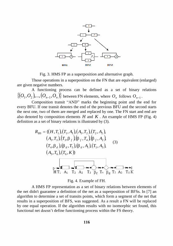
116
Fig. 3. HMS FP as a superposition and alternative graph.
Those operations in a superposition on the FN that are equivalent (enlarged)
are given negative numbers.
A functioning process can be defined as a set of binary relations
nn OOOO ,,...,, 121 between FN elements, where nO follows 1nO .
Composition transit “AND” marks the beginning point and the end for
every BFU. If one transit denotes the end of the previous BFU and the second starts
the next one, two of them are merged and replaced by one. The FN start and end are
also denoted by composition elements H and K . An example of HMS FP (Fig. 4)
definition as a set of binary relations is illustrated by (3).
,,,
,,,,,,,,
,,,,,,,,
,,,,,,,,
663
35154
24331
2221111
KTTA
ATATT
ATTTA
ATTAATTHR
ddd
fff
BS
(3)
Fig. 4. Example of FH.
A HMS FP representation as a set of binary relations between elements of
the net didn't guarantee a definition of the net as a superposition of BFSs. In [7] an
algorithm to determine a set of transits points, which form a segment of the net that
results in a superposition of BFS, was suggested. As a result a FN will be replaced
by one equal operation. If the algorithm results with no isomorphic set found, this
functional net doesn’t define functioning process within the FS theory.

117
A directed search algorithm (DSA) is applied to finding optimal decisions
in HES "INTELLECT-3". It's used within the general technique of consecutive
analysis of alternatives with stepwise designing of partial solutions [4]. The specific
stepwise design algorithm is defined by the rule for selecting partial solutions
(subnets) , which should be developed at each step, and a set of tests , that
eliminates the subnets which can not be completed to the optimal ones.
Requirements for optimality (OR) and feasibility of partial solutions (FR) are used
as a set of tests . The general scheme of DSA for FN within the technique of
consecutive analysis of alternatives is the following:
zrrrrr OxyxyxyDSA 122221111ˆ,,,...,,,,ˆ
(4)
where kj Oy is a chosen operation kO .
FN designing in HES "INTELLEKT-3" can result in common (coinciding) segments (Fig. 6), if alternative segments of functioning (Fig. 5) were defined.
Fig. 5. FN with an alternative segment.
Fig.6. Common segments in FN.
The general scheme for finding optimal solution includes building AG,
which considers all alternative segments of functioning. A FN can consist of
numerous nodes with the same operation alternatives, i.e. the same set of parametric

118
alternatives. Fig. 7 shows AG for the FN presented in Fig. 5. In HES
"INTELLEKT-3" before building AG a FN is preliminary analyzed if its alternative
segments have common parts. And AG later is formed considering these common
parts (Fig. 8). Common parts in AG result in DSA modification. If EQR indexes are
evaluated in a node that is defined as common, the partial solution found in this
node, is retained. This solution will be taken if needed, avoiding double calculations.
Fig. 7. Alternative graph for a FN with an alternative segment.
Fig. 8. AG for a FN with common parts
HES "INTELLEKT-3" allows to control DSA bypass in both manual and automatic mode. In automatic mode a rough estimation of complexity is made in case this sequence is chosen by DSA [4, 8].
Default bypass for the example shown in fig. 5 is illustrated in (5), an alternative is in (6).

119
321 ,, BFSBFSBFSV , (5)
341 ,, BFSBFSBFSV (6)
For the example considered there is a bypass (7) and (8):
231 ,, BFSBFSBFSV , (7)
431 ,, BFSBFSBFSV (8)
An AG which considers coinciding segments for such enumeration alternative will have a minimal number of nodes (Fig. 9).
Fig. 9. Alternative graph with minimal number of nodes
IV. CONCLUSION
The paper considers techniques for automation of designing human-machine systems functioning processes based on functional-structural theory and generalized structural method suggested by prof. A.I. Gubinsky. Isomorphic methods for HMS FP defining based on binary relations between elements included in a functional net and superposition of BFS were discussed. An algorithm determining segments of functional net that could be represented as a superposition of BFS was described. A hybrid expert system implementing the techniques described was presented.
REFERENCES
[1] A.I. Gubinsky. Nadezhnost` i kachestvo funktsionirovaniya ergaticheskikh system
[Reliability and quality of ergatic system functioning]. Leningrad, Nauka, 1982. - 270 p. (In Russian).
[2] А.I. Gubinskiy, V.G Evgrafov. Informatsionno-upravlyauschie cheloveko-mashinnie sistemy: Issledovaniye, proektirovaniye, ispytaniya. Spravochnik [Control and information human-
machine systems. Research, design, testing. Guide]. Мoscow, Mashinostroeniye, 1993. - 528 p. (In
Russian).

120
[3] А.I. Gubinskiy, V.G Evgrafov. Ergonomicheskoye proektirovaniye sudovyh system
upravleniya [Ergonomic design for ship control systems]. Leningrad, Sudostroeniye, 1977. - 224 p. (In
Russian). [4] M.G. Grif, E.B. Tsoy. Avtomatizatsiya proektirovaniya processov funktsinirovaniya
cheloveko-mashinnyh system na osnove metoda posledovatelnoy optimizatsii [CAD technique for
human-machine systems based on sequential optimization method]. Novosibirsk, NGTU, 2005. - 264 p. (In Russian).
[5] A.V. Zaykov, S.A. Kochetov, M.G. Grif. Metody i sredstva proektirovaniya processov
funktsionirovaniya cheloveko-mashinnyh system na osnove fumktsionalno-strukturnoy teorii [Algorithms and techniques for optimal design of Human-machine systems functioning processes based
on functional-strucural theory] // Nauchniy vestnik NGTU [NSTU Science Bulletin] , 2008. 3(32).
Novosibirsk, NSTU, pp. 95-110. (In Russian).
[6] E.V. Geniatulina. Metody proektirovaniya i modelirovaniya v zadachah optimizatsii
processov funktsionirovaniya cheloveko-mashinnyh system [Design and modeling methods for optimization of HMS functioning]. E. V. Geniatulina, M. G. Grif, Trudy SPIIRAN [SPIIRAS Proc.] ,
2014. 5(36), pp.151-167. (In Russian).
[1] M.G. Grif, S.A. Kochetov, E.B. Tsoy. Strategii proektirovaniya mnozhesyva alternativ v zadachah optimizatsii na osnove funktsionalno-strukturnoy teorii [Functional-structural
theory based strategies for designing a set of alternatives in human-machine systems optimization
problems] // Doklady Akademii nauk vishey shkoly Rossiyskoy Federatsii [Reports of the Academy of Sciences of the Higher School, Russian Federation] , 2015. 4(29), pp. 44-51. (In Russian).
[2] M.G. Grif, S.A. Kochetov S.A., N.D .Ganelina. Functional -Structural Theory
Based Techniques for Human-Machine Systems Optimal Design//13 International Scientific -Technical Conference on Actual Problems of Electronic Instrument Engineering (APEIE) – 39281: proc. Russia,
Novosibirsk, 3–6 October 2016. - Novosibirsk, 2016. - Vol. 1. Part 2. – pp. 494-497.

121
Learner Centered Learning: Development of
Supportive Environment and Its Evaluation
Uranchimeg Tudevdagva1, Wolfram Hardt
2
1,2TU Chemnitz
chemnitz.de Abstract—this paper discusses on supportive learning environment for
learner centered learning approach. The approach is not new term in education systems,
but with technological rapid development and with new generation of learners we have
to review this approach with added values. Learner centered learning has many factors
for practical cases. One the important factor is learning environment. If we cannot
provide corresponding environment for this approach implementation of this idea will
not run in practice successfully. Here we describe our idea about “supportive” learning
environment for learner centered learning. Learner should be able to design and plan
personalized study plan during own study. Because each learner has personal skill and
individual methods to learn. Pre-defined study plan and static designed linked courses
cannot support learner centered learning approach. We tried to wake up this problem
in light and establish supportive learning environment where learner really can plan
personalized study plan and can finish study in own time successfully.
Keywords—study plan; credit point; student centered learning; learner oriented
learning; learning environment;
I. INTRODUCTION
Learner Centered Learning (LCL) is by definition not new approach in
teaching and learning. Nevertheless, with development of technologies, with change
of learners’ attitude and behaviors this approach facing to update.
Existing various similar approaches for LCL. For example, student
centered learning, student oriented learning, personalized learning, learner centered
training, learner centered education, learner centered pedagogy etc.
Researchers are published many works relating to above listed approaches,
and discussing about different accepts of LCL [1-6]. For example, Debec studied
effectiveness of LCL approach for Teaching an Introductory Digital Systems
Course [1-2], Matukhin and Bolgova used LCL approach to teach foreign language
[3], Randall and Jane discussed on learner centered pedagogy issues [4]. This list
can be continuing longer. Reading confirmed that all researchers are summarizing
that LCL is important approach for modern and further education system.
Here we would like to discuss about supportive learning environment for
LCL. Our solution for supportive learning environment came from planning of

122
teaching and design of curricula for offering academic program. Usually
universities designing their academic semesters quite early before to start academic
year. Schedule of offering courses depend on teaching hours for professors and
learning hours for students in curricula. Learner should follow schedule from
university and have to select courses, which are offering in that academic semester.
Each course has pre-condition to select that course. This can be some knowledge,
practical hours or other course. That means learner simply cannot select any course,
which he/she want to listen in coming academic semester. To select course learner,
have to fulfil pre-defined condition of course.
We see here just some most visible conditions and way to design study
plan of learner. There are many other conditions and situations, which are
influencing to selection and designing of learners’ study plan.
Focus of this paper is to discuss curricula and credit points of courses and
planning of offering courses for academic year. These two factors are part of many
factors, which are important to develop “supportive” learning environment for LCL.
II. CREDIT POINTS
A. Curricula and credit points
First, let us look into credit points (CP). This is very important element of
any level of higher education. To fill requirement for degree learner, have to collect
credit points. No expected credit points, no chance to get degree!
Fig.1. shows us way from enroll to graduation.
As usually, every university has traditional plan for academic degrees.
Fig.1 shows, study plan for “Bachelor” degree as finite state machines. If any
person enrolled to university this means learner has limited time to finish it.
Moreover, we visualized it via states of finite state machine. Learner have to go
through of all these states to get degree.
S0 state denoted for freshman. Freshman is any person who received
acceptance to enroll university. By pre-defined plan (Fig.1) learner, have to collect
at least 60 CPs in each academic year. If learner could collect needed CP in each
year by predefined plan (traditional expectation of administration), he/she can reach
in planned time state S7. S7 state defines as diploma work or final exam for
graduation. Between S0 and S7 we have six more states. These states are defining
academic semesters where learner have to collect according CPs. S1 and S2 states
are defines first academic year. If learner can collect, 60 CPs in states S1 and S2

123
then can move to state of next year. If not enough CPs then have to stay in states of
first year. S3 and S4 states are defines second academic year. S5 and S6 states are
defines third academic year. After completion of credits learner will receive, right
to select diploma subject. This state is state S7. Main condition to fit traditional plan
of study (Fig.1) is to collect corresponding credits in giving time. Else, this picture
will change very much.
Fig.2. Change in pre-defined plan
For example, learner could not collect necessary CPs in second year of
study. In that situation, states of study plan can be change dramatically. Will appear
new states (S1’, S2’ and S3’) with new way and no body cannot estimate time to
finish study successful (Fig.2). These views (Fig.1-2) could be helpful to learners to
follow their study plan. If learner wants to finish study in good time should keep in
mind these states and try fit pre-defined time. Our target of research is design
flexible environment for individual planning but in expected time to graduation.
As usually, courses has different hours in curricula definition and relating
to this CPs for such us courses are different.
Fig.3. Credit points and study planning
Let us see to pre-defined study plan from different view. In Fig. 3 shows
pre-defined plan as boxes. Each box consists of 2 academic semesters (S1 and S2).
Here we can see one basic problem for learners. Administration defined total CPs,
which have to collect learner during one academic year. For example, here total

124
summary should be 60 CPs, but offering courses has different CPs. Main challenge
of student (learner) is have to look total CPs and decide which course want to learn.
Fig. 3 shows how not easy to puzzle courses together to fit expecting CPs.
Sometime have to do decision about CPs or course! If learner will collect, less than
requested then box will have leer spaces. By means cannot move to next box.
Opposite, if learner collected credits more than requested then again it is not fitting
to pre-defined box.
TABLE I. Study plan by credit points
In Table 1 visualized above discussed problem. Different CPs of courses
are influencing to design of individual study plan a lot. Main reason is total CPs
should fit to pre-defined sum and student have to look to not only content of course
always have to keep in mind how much credit will get from this course. By means,
this type of planning is not enough flexible for LCL. If universities will not
illuminate this difference between courses, we cannot provide “supportive” learning
environment for LCL.
Some universities already started to solve this problem. For example, TU
Chemnitz since 2010 worked on this issue and Faulty of Computer Science reached
some agreement between professors. Now all offering course from this faculty has
same credit points = 5. This made a lot of progress for individual planning for

125
students. It gave to students more freedom to select course by own interest and for
future target. How solved different hours of courses, how could fit all courses into 5
CPs? Smart solution come with e-learning. E-learning part included to courses,
which had, less than PCs in previous curricula.
But here we still have some administration problem, even CPs are same for
all courses. In TU Chemnitz for bachelor study student have to collect 60 credits
per year. Offering courses has different curricula and following this each course has
different CP! Here coming in light problem. What is the problem? Problem is
student have to plan own study plan with balance. What means balance? Should
collect 30 PCs in each semester and totally 60 PCs can be collected by an academic
year. If learner collected 45 PCs in first academic semester and 15 points in next
academic semester, then administration issue not accepting it (Fig.4.) [7].
Fig.4. Imbalance: Not accepting
This problem can solve if we can make more flexible study plan for
learners. Pre-defined study plan like in Fig.1 should be more flexible and student
could have freedom to finish early his study or a bit later than planned in this
manner.
B. Personal planung of courses
Every university defining teaching hours plan and publishing it before to
start academic semester. Idea is to support learner to design their study plan as
personal case.
Fig.5 shows online study planner for students of TU Chemnitz. This is
view of Master students for Automotive Software Engineering program.

126
Fig.5. Study planner
Let us explain important points of figures.
1. Number one shows to 5/20. This is credit points which have to collect
learner in giving semester. 20 means total number of CPs and 5 of them pre-defined
requested course which learner “have to” include to selection. Remaining 15 CPs
learner can select from offered list.
2. Here we can see crossed box, that means this course is already in
selection. This is the required pre-defined course. Learner cannot change this state.
3. Yellow triangle with red ! shows planning is not finished. If learner
selected less or more credits, then us needed this symbol will stay visible. If plan is
fitting to expectation, then this symbol will vanish.
4. Flag of countries shows language of offering course. Some course is
only in German or English. Some of them is possible to learn in both languages.
In Fig.5 some course: Network security, Self-Organizing network and
Mobile networks has not 5 CPs. Because these courses are courses which offering
from other faculties. That means not all faculties in TU Chemnitz updated curricula.
There are still existing many courses which have different CPs.
III. SUPPORTIVE LEARNING ENVIRONMENT
As we mentioned in Introduction section many researchers agreed that
LCL is one of correct way for teaching and learning. The successful
implementation of LCL approaches need corresponding environment. In second
section, we discussed about case of TU Chemnitz. In this section, we will discuss
about need of evaluation and evaluation method.

127
A. Need of evaluation
Why we need evaluation? Establishment of supportive environment for
LCL is costly and long process. No one university cannot manage it in short time.
For long-term project, we need corresponding evaluation. Evaluation process will
help to us to recognize pluses and limitations, via evaluation we can define early
our weak points and can improve in early.
B. Evaluation method
For evaluation existing various type of methods. We will apply structure
oriented evaluation model for this evaluation. Originally, this method developed for
evaluation of e-learning [8-9].
The quantitative models for the assessment of e-learning quality
considered usually are additive models. That means, depending on the considered
aspects, which are measured based on a defined scale, a linear function containing
corresponding weight factors is used like, e.g.,
𝑄 = Σ 𝑎𝑖 𝑥𝑖
Here denote 𝑎𝑖 , 𝑎𝑖 > 0, given weight factors for the obtained measure
values 𝑥𝑖 , 𝑖 = 1, … , 𝑘, for the considered aspects. The advantage of this formula is,
it is very easy. The disadvantage is that the choice of proper weight factors is
subjective. Moreover, positive evaluation values can be obtained even in such cases
if the targets of certain quality aspects have been failed. A possible logical inner
structure of target structures remains out of consideration.
In contrast to linear approaches, we develop here a measure theoretical
model for the assessment of an e-learning program. We consider an e-learning
program whose quality is determined by 𝑘, 𝑘 ≥ 1, several aspects or characteristics
𝑀1, … , 𝑀𝑘 . We assume that the quality of the single aspects can be measured by
means of a given scale where the corresponding observation variables are ordinal or
metrical ordered variables. Our aim is to develop an evaluation model for e-learning
programs whose quality characterized as above by 𝑘 several aspects 𝑀1, … , 𝑀𝑘 .
For it we will construct a corresponding measure in sense of general measure theory.
This requires in the context considered here two steps. First we will construct 𝑘 corresponding efficiency measure spaces for description of quality of single aspects
𝑀1, … , 𝑀𝑘. After that we will combine these spaces to a corresponding product
space. This space will describe the considered aspect structure as a whole. The via
the obtained product space defined product measure will be then our quality
measure for evaluation of an e-learning program. For the implementation and
application of our assessment approach, the paper rounded off by a statistical
procedure for the estimation of scoring values for target structures based on adapted
assessment checklists.

128
The advantage of the model considered here in comparison with linear
models is that by the multidimensional consideration via the product measure the
logical structure of a target structure evaluated as a whole [9].
C. Design of goal structure for evaluation
Based on structure oriented evaluation model we have to define main and
sub goals of evaluation.
Main goal of evaluation is establishing supportive learning environment
for LCL. How we can reach this main goal? There is some fact which we have can
use to reach our main goal.
Courses should have same credits.
A course should be possible to select in every academic semester.
Learner able to finish study early than defined date.
Main goal reached if each of this defined facts fulfilled. Therefore, we can
define these facts like our sub goals. Each sub goal should be successful
implemented to reach our main goal. That means by structure oriented evaluation
model idea this structure we can define like serial structure (Fig.6).
Fig.6. Goal structure of evaluation
By calculation rule of structure-oriented evaluation model if any of these
sub goals cannot reach own target main goal of evaluation will evaluate as failed.
IV. CONCLUSION AND DISCUSSION
In conclusion we can summarize that learner centered learning is one of main
approach of modern and future education. Relating to dynamic change of
technology and behavior of young generation educators and universities have to
support more individual and personalized study plan of learners’. As case study,
showed universities try to synchronize credit pints of offering courses. Then this
will be open new opportunities not only for learners this can be useful for
universities to develop joint or flipped study programs together.
For discussion, we are highlighting several questions: How we can manage better
our administration issues to support learner centered learning? How we can
recognize problems relating to culture different behavior of our learners? How we

129
can use artificial intelligence and other well developing research results into learner
centered learning?
We are looking to your valuable feedback and comments to our on-going
work.
REFERENCES
[1] Piote Debies, “Effective Learner-Centered Approach for Teaching an
Introductory Digital Systems Course”, IEEE Transactions on Education, Vol. 61,
Iss.1, pp.38-45, 2018. DOI: 10.1109/TE.2017.2729498
[2] E. Cetin, C. Wijenayake, V. Sethu, E. Ambikairajah, "A flipped mode
approach to teaching an electronic system design course", Teaching Assessment
and Learning for Engineering (TALE) 2017 IEEE 6th International Conference, pp.
223-228, 2017.
[3] D.Matukhin, D.Bolgova, “Learner-centered Approach in Teaching
Foreign Language: Psychological and Pedagogical Conditions”, XVth International
Conference on Linguistic and Cultural Studies: Traditions and Innovations, Journal
of Procedia - Social and Behavioral Sciences, Vol. 206, pp.148-155, 2015.
[4] Randall M. Moate, jane A.Cox, “Learner-Centered Pedagogy:
Considerations for Application in a Didactic Course”, The Professional Counselor,
Vol. 5, Issue 3, pp. 379–389, 2015.
[5] A. Reinert, N. Vollmann, M. Heyder, and W. Krautschneider, “New
teaching approaches and student motivation lead to documented gains in
engineering education,” in Proc. IEEE Front. Educ. Conf., Madrid, Spain, 2014, pp.
1–4.
[6] A. Lukkarinena, P. Koivukangasa, and T. Seppälä, “Relationship
between class attendance and student performance,” Proc. Soc. Behav. Sci., vol.
228, pp. 341–347, Jul. 2016.
[7] W.Hardt, U.Tudevdagva, “Adaptivity and Digitalisation Enables
Learner Centred Learning”, Journal Open Access Government. - pagesuite,
November 2017, pp. 176-177, ISSN: 2055-7612, 2017.
[8] Source for figure: www.itnews.com.au
[9] U.Tudevdagva, W.Hardt, A new evaluation model for eLearning
programs, Dezember 2011, Chemnitz.
[10] U.Tudevdagva, “Structure oriented evaluation model for E-Learning”,
Chemnitz, Univ.-Verl., Vol.14, 2014

130
Based on the improved RNN-CRF named entity
recognition method
Jinbao Xie1, Baiwei Li
2, Yajie Wang
3, Yongjin Hou
4, Kelan Yuan
5, Youbin
Yao6
1,2,3Harbin University of Science and Technology (HUST)
4China Telecom
5,6Harbin International Technology Transfer Service Center
Abstract—This paper proposes a method based on the improved RNN-CRF for the
problem of Chinese named entity identification. It uses the Gated Recurrent Unit
(GRU) network to extract the sentence features of the marked part of the corpus, and
then integrates the conditional random fields (CRF) for entity tagging to complete the
named entity recognition. The network performs feature extraction. The GRU network
has the characteristics of less parameters, strong fitting ability, and high training speed.
It reduces the time spent on training large-scale data, and is used in combination with
CRF to mark a location in the CRF. Can use the marked information to get better
Chinese entity recognition effect.
Keywords- GRU, named entity recognition, CRF
I. INTRODUCTION
With the rapid development of Internet technology, humans have become
accustomed to acquiring a large amount of knowledge from the Internet. However,
with the continuous growth of network resources and the diversity of resources,
methods for acquiring knowledge from the Internet have stagnated, so how to
obtain information efficiently from the Internet And the discovery of new
knowledge becomes more urgent. Named entity recognition has become essential as
a basic task in the field of natural language processing. In recent years, computer
performance has been continuously improved, and artificial intelligence has
developed rapidly. The method of named entity recognition based on machine
learning has become the focus of research on named entity recognition. Deep
learning has also made some progress in research on named entity recognition.
Named entity recognition is a fundamental part of many natural language
processing applications. Named entity recognition is a sub-task of information
extraction in the field of natural language processing. From the text data, the
position of the entity is found and the entity category is correctly divided. For

131
example, question answering systems, automatic machine translations, etc. are all
based on the further research of named entity recognition.
Named entity recognition is a research hotspot in the field of natural
language processing. From the early methods based on lexicon and rules, to the
traditional machine learning methods, and deep learning methods in recent years,
the recognition effect is constantly improving. The neural network-based entity
recognition model can process natural language processing of network resources
from the perspective of algorithm knowledge more effectively by using natural
language grammar, semantics, and other information, what’s more it can open up
neural network for the mining and representation of algorithm knowledge.
In this paper, we use the improved neural network RNN-CRF method to
study the method of Chinese named entity recognition. Recurrent neural networks
(RNNs) have been widely used in many natural language processing applications.
An improved RNN network is proposed, which uses GRU (Gated Recurrent Unit)
instead of RNN. Its purpose is to solve the deficiencies of RNN in the study of
named entity recognition, and to capture long-distance impact in the sequence. To
better achieve the effect of named entity recognition.
II. NEURAL NETWORK MODEL STRUCTURE
A.GRU Structure
This article uses the GRU (Recursive Recurrent Unit) of a recursive network recursive neural network. The GRU is an improved recurrent neural network (RNN). The state and output of a GRU (Gated Recurrent Unit) network are calculated as follows:
1( ) Z z
t tz U x W s (1)
1( ) r r
t tr U x W s (2)
1tanh( ( * )) h h
t th U x W s r (3)
1(1 )* * t ts z h z s (4)
Where t is the sequence length, z is the update gate of the GRU, r is the reset
gate of the GRU, and h is the hidden state at time t. * denotes multiplying by
elements and multiplying the elements one by one to get a new vector.
z and r have the same form, but the parameters are different. The parameters U
and W need to be learned during the training of the sample. r and z together control
the new hidden state ( ts )from the previous hidden state ( 1ts ) calculation. z is used
to control the extent to which the state information at the previous time was brought
into the current state. The value of z is greater. Explain that the status information
from the previous moment brings in more. r is used to control the degree of

132
ignoring the status information at the previous moment, and the smaller the value of
r, the more ignoring it is. Its structure is shown in Figure 1:
*
th%
1th
-
tx
Wg s
tr
1th
-
Reset Gate
W
tx
t anh
1th
-
tx
zW s 1-
*1th
-
1t
z-
+
*tz
Update Gate output
Fig. 1. The Gated Recurrent Unit model structure diagram
tx denotes the input of model time t. The output of GRU at time t is
defined as th . This expression also contains the above information and the following
information. It is applicable to the task of named entity identification with many
types of labels.
Conditional Random Field (CRF) is an algorithm commonly used in the
field of natural language processing in recent years for named entity recognition.
Some feature functions with artificial definitions are used as feature templates for
name entity recognition research. For sentence given in the sentence In terms of
location, different feature templates can be combined to form a new feature template.
Using feature templates for sentence tagging, CRF has limitations on named entity
recognition and the overall effect is not ideal. This paper proposes an improved
model which combine the RNN and CRF together CRF. Its purpose is to solve the

133
limitations of CRF in the study of named entity recognition, which helps to achieve a
better effect of named entity recognition of named entity recognition.
B.Named Entity Recognition Model
The output of the GRU at time t is denoted as th .The labeling result at
time t is directly predicted and a named entity recognition model is established. The
structure of the model is shown in Figure 2:
美 丽 中 国One hot vector
x1 x2 x3 x4look-up layer
h1 h2 h3 h4
M1
O O B-LOC I-LOC
Forward GRU
backward
GRU
CRF layer
h1 h2 h3 h4
M2 M3 M4 output
Figure 2 Overall model diagram
As shown in Figure 2, this paper first pre-processes the corpus and marks
part of the corpus. In the pre-processing process, it first uses jieba firstly to cut
words, segment words, and then use Word2vec to pre-train some of the segmented
corpora. Then each word is divided into one line for labeling. This article uses the
BIO tagging set in the labeling process, ie B-PER represents the first name of the
person's name, I-PER represents the first name of the person's name, B-LOC
represents the first name of the place name, I-LOC On behalf of non-first place
names, B-ORG represents the first name of the organization, I-ORG represents the

134
non-headword of the organization, and O represents the word is not part of the
named entity.
Then each word in the sentence is represented as a one-hot vector; in
natural language processing, because machine learning cannot receive the corpora
as input directly, it is usually necessary To digitize the linguistic number firstly, and
the word vector is used to carry out the words in the language. In way of
mathematics. In this paper, the one-hot vector is used to represent the word vector,
and the character is transformed into the corpora with the unit of the sentence, and
each word in the sentence is mapped from the one-hot vector to the low-
dimensional dense word vector using the randomly initialized embedding matrix.
As a neural network input.
Then the word vector is input into the GRU network for feature extraction
and the matrix M for extracting sentence features is obtained through GRU network
training. Finally, the matrix M access conditions obtained through neural network
GRU training are tagged with the sentence level of the airport CRF layer. The training process of the CRF model is divided into two parts. The first part is the establishment of the feature function set, and the second part is the estimation of model’s parameter, which is the weight of the calculation function. The process of annotating a location by the CRF can use the labeled information and use Viterbi decoding to obtain the optimal sequence. Denote the tagged sequence of sentence
length n with 1 2 3( , , ,..., ) ny y y y y , and the score of 1 2 3( , , ,..., ) nx x x x x for length
n is:
1
11 1( , ) , ,
n n
i i i ii iscore x y M y Ay y (5)
Among them, M is the characteristic matrix M obtained through the GRU
network, and A is the transition matrix A of the CRF. By performing exponentiation
and normalization on this score, the probability value ( )p x y of the annotation
sequence can be obtained as follows:
'
exp( ( , ))( )
exp( ( , ')) y
score x yp x y
score x y (6)
In the model training, the likelihood ratio is selected by the maximum
likelihood function. The log likelihood for the training sample ( , )x y is as follows:
'log ( ) ( , ) log( exp( ( , '))) y
p y x score x y score x y (7)
In the model prediction process, a dynamic programming Viterbi algorithm
is used to solve the optimal decoding path. The highest probability y is shown in
formula:

135
'
arg max ( , )y
y score x y (8)
III. EXPERIMENTS AND RESULTS
In the experiment, In order to measure the entity recognition’s effect in the model objectively, the test corpora were annotated and the results were statistically calculated under the same environment. Through the analysis and comparison of a large number of test results, the results show that the improved neural network can be well applied to the named entity recognition tasks. The marked effect of the model is better than the RNN model.
This article uses the news corpus marked in January 1998 by the People's Daily as an experimental corpus. Because in the named entity Recognition mission , this article takes the recognition effect of the Chinese name, place name and organization name as the main evaluation objects in the experiment. At the same time, precision, P, Recall, R, and F1 measure values (F1-score, F) are used for statistical evaluation of names, place names, and institution names. The calculation method is shown in formula:
TPP
TP FP (9)
TPR
TP FN (10)
2
2
TPF
TP FP FN (11)
Among them, TP indicates that the positive class is predicted to be positive (True Positive), FN indicates that the positive class is predicted to be negative (False Negative), FP indicates that the negative class is predicted to be positive, and TN indicates that the negative class is predicted to be negative The number of classes, F, is the comprehensive evaluation index of precision rate and recall rate.
Through analysis and comparison of a large number of test results, the results
show that the modified GRU-CRF model can be well applied to named entity
recognition tasks, and the model's labeling effect has better recognition effect. Long
Short-Term Memory (LSTM) is a neural network with good effect on named entity
recognition. This paper compares the GRU-CRF model with LSTM-CRF model.
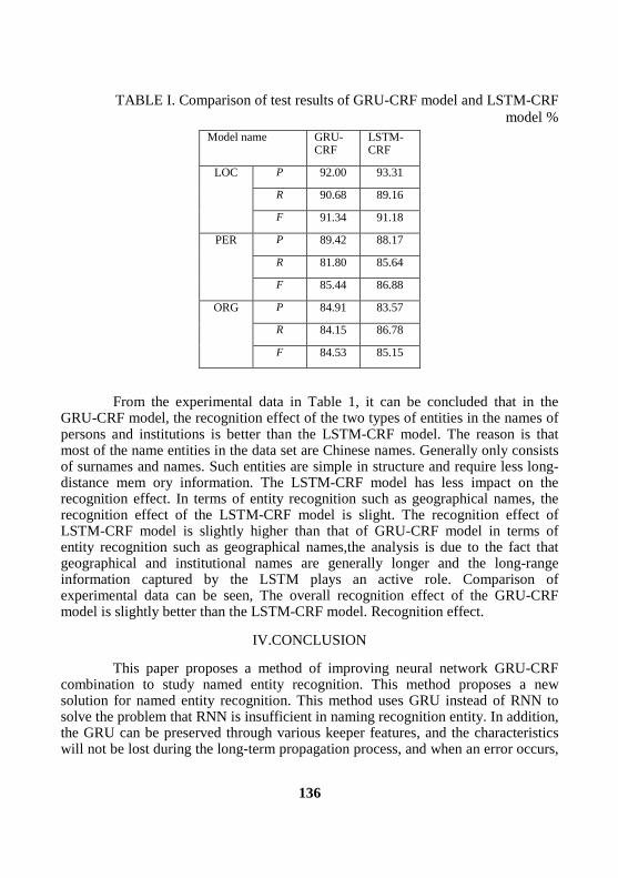
136
TABLE I. Comparison of test results of GRU-CRF model and LSTM-CRF
model % Model name GRU-
CRF LSTM-CRF
LOC P 92.00 93.31
R 90.68 89.16
F 91.34 91.18
PER P 89.42 88.17
R 81.80 85.64
F 85.44 86.88
ORG P 84.91 83.57
R 84.15 86.78
F 84.53 85.15
From the experimental data in Table 1, it can be concluded that in the GRU-CRF model, the recognition effect of the two types of entities in the names of persons and institutions is better than the LSTM-CRF model. The reason is that most of the name entities in the data set are Chinese names. Generally only consists of surnames and names. Such entities are simple in structure and require less long-distance mem ory information. The LSTM-CRF model has less impact on the recognition effect. In terms of entity recognition such as geographical names, the recognition effect of the LSTM-CRF model is slight. The recognition effect of LSTM-CRF model is slightly higher than that of GRU-CRF model in terms of entity recognition such as geographical names,the analysis is due to the fact that geographical and institutional names are generally longer and the long-range information captured by the LSTM plays an active role. Comparison of experimental data can be seen, The overall recognition effect of the GRU-CRF model is slightly better than the LSTM-CRF model. Recognition effect.
IV.CONCLUSION
This paper proposes a method of improving neural network GRU-CRF combination to study named entity recognition. This method proposes a new solution for named entity recognition. This method uses GRU instead of RNN to solve the problem that RNN is insufficient in naming recognition entity. In addition, the GRU can be preserved through various keeper features, and the characteristics will not be lost during the long-term propagation process, and when an error occurs,

137
only the weights that cause the error items need to be modified. The GRU has fewer parameters and the training speed is faster. The characteristics of the training time are shortened. The number of samples required during the training process is small. This solves the problem of insufficient corpora in the named entity recognition. The GRU has efficient and rapid training characteristics for the training corpora, and then combines CRF with sentence sequence annotation. Named entity recognition has a good effect.
REFERENCES
[1] Huang Z, Xu W, Yu K. Bidirectional LSTM-CRF models for sequence tagging[J]. arXiv
preprint arXiv:1508.01991, 2015.
[2] Dong C, Zhang J, Zong C, et al. Character-Based LSTM-CRF with Radical-Level
Features for Chinese Named Entity Recognition[C]//International Conference on Computer Processing of Oriental Languages. Springer International Publishing, 2016: 239-250.
[3] Ma X, Hovy E. End-to-end sequence labeling via bi-directional lstm-cnns-crf. arXiv
preprint arXiv:1603.01354, 2016. [4] Chiu J P C, Nichols E. Named entity recognition with bidirectional LSTM-CNNs. arXiv
preprint arXiv:1511.08308, 2015.
[5] Matthew E. Peters, Waleed Ammar, Chandra Bhagavatula, Russell Power. Semi-supervised sequence tagging with bidirectional language models. ACL, 2017.
[6] WANG G Y. Research of Chinese Named Entity Recognition.Based on Deep
Learning[D]. Beijing:Beijing University of Technology,2015:33-38. (in Chinese) [7] FENG Y H, YU H, SUN G, et al. Domain-specific Terminology.Recognition Method
Based on Word Embedding and CRF[J].Journal of Computer Applications, 2016, 36(11): 3146-3151. (in
Chinese)
[8] Cho K, Van Merrienboer B, Gulcehre C, et al. Learning Phrase
Representations using RNN Encoder-Decoder for Statistical Machine Translation.
Computer Science, 2014

138
Numerical Optimization of Automatic Control System Vadim A. Zhmud
1, Lubomir V. Dimitrov
2, Jaroslav Nosek
3, Hubert Roth
4
1Novosibirsk State Technical University (NSTU)
2 Technical University of Sofia 3 Technical University of Liberec
4University of Siegen
Abstract – The problem of control object with the use of feedback loop is
extremely relevant, because only this method provides for the accurate control.
The most difficult part of the task is design of regulators. Mathematical
methods cannot be used for object containing delay link or nonlinear elements.
For such complex objects the most effective method is numerical optimization.
Due to the exixtanse of the smart software, sach as VisSim, this problem can be
easily resolved without deep knowledges in the field of theory of feedback
control. This paper gives most impotrant information about the numerical
optimization of regulators by means of software VisSim.
Keywords—control, regulator, PID, numerical optimization, modeling
I. INTRODUCTION
Object control with the help of feedback is one of the key methods of
robotics. It is also used in all automation devices. Modern engineering is
inconceivable without such systems [1–10].
The main difficulty in designing such systems is the calculation of the
regulator. This paper gives an automatic method for calculating regulators, which
does not require deep special mathematical skills and deep knowledge in the theory
of automatic control. The designer only needs to get acquainted with the very
foundations of this theory and the methods of numerical optimization in practice.
A typical block diagram of the automatic control system is shown in Fig. 1.
For the most common case of W3(s)=1 and without considering the noise of the
sensor, the loop is simplified to the structure shown in Fig.2.

139
Fig.1. Structure for calculation of ACS
Fig.2. The Simplified Structure of ACS
The most commonly used regulator contains proportional, integrating and
derivative links. The transfer function of such a regulator, called the PID-regulator,
is given by the ratio (1):
sKs
KKsW D
IPР )( . (1)
Here, KP, KI, KD are constant coefficients which are required to determine
with the procedures as a result of numerical optimization.
Another form of regulator (1) is:
s
sKKsKsW
ДИП
Р
2
)(
. (2)
More sophisticated regulators may include additional derivative and (or)
integration. For example, if the regulator contains both these additional channel, its
transfer function might look like this:
2
22
2)( sKsKs
K
s
KKsW ДД
ИИПР . (3)
Such regulator is named PI2D
2 or PIIDD-regulator.
II. METHOD FOR THE DESIGNING OF REGULATORS
Among the methods of solving these problems, the following ones can be
specified:
1. Analytical (mathematical) methods.
2. Tabular methods.
3. Empirical tuning.
4. Mathematical modeling for the study of properties of the system.
5. Numerical methods for optimization of the locked loop model or a
real system with the object based on built-in routines of modern software packages
for modeling and mathematical calculations, such as VisSim.

140
Numerical optimization is the most effective method of regulators tuning,
if the object model is stationary and known with sufficient accuracy. It uses a
mathematical modeling (simulation) of the system that contains the object and the
regulator.
III. PROCEDURE FOR THE AUTOMATIC OPTIMIZATION OF
REGULATORS
To run optimization in VisSim, a developer should do the following things.
1. Setting of one or more optimized parameters using the “parameter
unknown” blocks.
2. Setting the initial (starting) values to each of these parameters, giving a
constant to the input of these blocks
3. Ensuring of the use of these parameters as regulator coefficients to be
optimized. For this purpose, it is useful to give them the names of functional
variables (for example, P, I and D are the coefficients of the proportional, integral
and derivative links). Assigned names should be used to call these functions as
appropriate gains. A developer can use multiplier blocks or directly blocks of gain
factors.
4. Ensuring of calculation of the cost function and sending of the result to
the “cost” block, which should be the only one in the project. For this goal, a
calculator is formed, the output of which is connected to the input of this block.
5. Providing of an indication of the optimization result, for which it is
advisable to use the value indicator block at the output of each of the “parameter
unknown” blocks.
In addition, it is possible, but not necessary, to reflect the value of the resulting
transient process on the oscilloscope block and the value of the cost function on
such a unit and (or) on the numeric value indicator unit.
IV. STRUCTURE FOR THE REGULATOR OPTIMIZATION
To optimize the regulator, it is required to apply a structure containing the
system model and a number of auxiliary modules. The model of the system includes
a regulator and an object, and other specific blocks can also be included.
In addition to the system model, the structure should contain:
1. Means of formation of test signals.
2. Means of indicating the results of optimization.
3. Means for calculating the value function.
4. Means of formation of initial values of parameters.
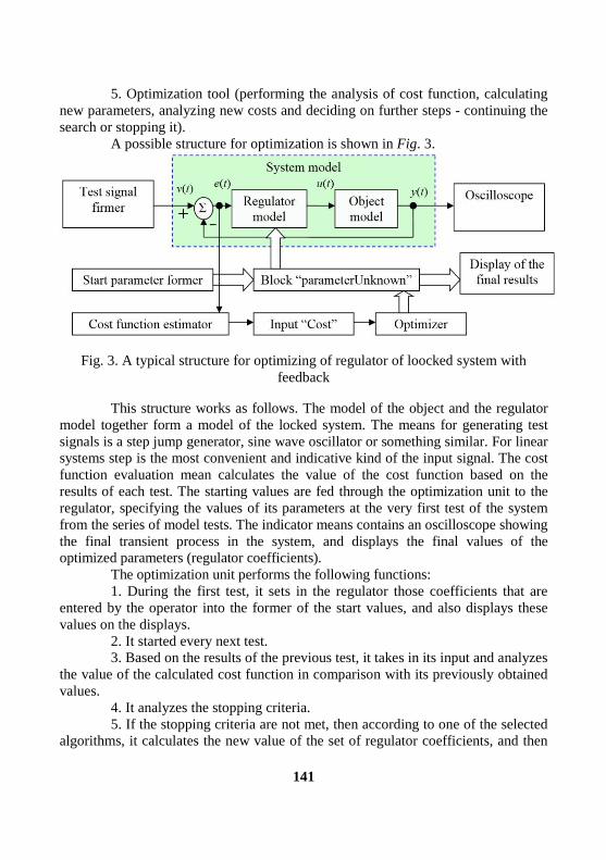
141
5. Optimization tool (performing the analysis of cost function, calculating
new parameters, analyzing new costs and deciding on further steps - continuing the
search or stopping it).
A possible structure for optimization is shown in Fig. 3.
Fig. 3. A typical structure for optimizing of regulator of loocked system with
feedback
This structure works as follows. The model of the object and the regulator
model together form a model of the locked system. The means for generating test
signals is a step jump generator, sine wave oscillator or something similar. For linear
systems step is the most convenient and indicative kind of the input signal. The cost
function evaluation mean calculates the value of the cost function based on the
results of each test. The starting values are fed through the optimization unit to the
regulator, specifying the values of its parameters at the very first test of the system
from the series of model tests. The indicator means contains an oscilloscope showing
the final transient process in the system, and displays the final values of the
optimized parameters (regulator coefficients).
The optimization unit performs the following functions:
1. During the first test, it sets in the regulator those coefficients that are
entered by the operator into the former of the start values, and also displays these
values on the displays.
2. It started every next test.
3. Based on the results of the previous test, it takes in its input and analyzes
the value of the calculated cost function in comparison with its previously obtained
values.
4. It analyzes the stopping criteria.
5. If the stopping criteria are not met, then according to one of the selected
algorithms, it calculates the new value of the set of regulator coefficients, and then

142
returns to the repetition of all operations starting from step 2. If the stopping criteria
are fulfilled, proceeds to step 6.
6. It selects the regulator coefficients corresponding to the lowest value of
the cost function.
The stopping criterion can be one of the following:
a) the number of iterations has exceeded the specified value;
b) it is established that further implementation of this algorithm will not
lead to a decrease in the value function by an amount exceeding the specified
permissible optimization error;
c) an error occurred that makes it impossible to continue the procedure, for
example, exceeding one of the parameters or one of the calculated values of the
largest permissible value (for different versions of the program this is 1028
– 1030
,
etc.).
The cost function calculated in the structure implicitly depends on the
regulator parameters and on the test actions generating the transient process, since
the error function of the system e(t) depends on these parameters. When solving the
problem of numerical optimization, it is required to find such values of the regulator
coefficients for which the cost function reaches a minimum value. Since the error in
the system depends on the regulator coefficients, the entire cost function will
depend on these coefficients. The solution of this problem is called the optimum, in
our case the minimum. It is necessary to distinguish between local and global
minima. Local minima are solutions in which small changes in any parameter cause
an increase in the cost function; however, this does not apply to big changes in
these parameters. The global minimum can be the only. This is the solution that
ensures the least value of the cost function for all parameters from the range of their
allowed values.
Various algorithms for finding the minimum can be applied. The
correctness of the choice of the optimization method depends on the properties of
the problem: the best method for one task may be the worst or completely
inapplicable for another task.After rounding of the obtained coefficients, it is
necessary to verify the admissibility of such rounding and the preservation of the
achieved type of transient processes (minor changes are allowed) and approximate
preservation of the value of the cost function. To do this, it is necessary to fill the
blocks of preset values by “copy-paste” method with the received parameters values
and round these parameters, then in the “optimization” menu one should uncheck
the “optimize” window, select the “remember graphs” checkbox in the oscilloscope
configuration menu and start the simulation again.
This method of verification is necessary to exclude a non-rough solution,
i.e., a solution that ensures a given quality only if the values of the parameters are
extremely accurately matched to their values.

143
The presence of a non-rough solution can arise in the case, for example,
when an object contains an unstable oscillatory link, for the stabilization of which
mathematical modeling suggests the introduction of a blocking filter tuned to the
same frequency in the regulator. Such a decision has no practical value, since its
implementation is impossible, and also because a sufficiently accurate identification
of such an object is also impossible, that is, an object with such properties is most
likely not exactly in accordance with the model used, but the implementation of the
regulator, most likely, does not coincide with the calculated regulator.
Example 1. Fig. 4 shows an example of a PID-regulator optimization
project for some linear object.
The most important principles of application of automatic optimization are
the following.
1. Not only the step of sampling in time, but also the simulation time
(duration) should be chosen reasonably. We should strive to ensure that the
transient process ends in approximately 70–80% of the simulation time. If the
transient process is not yet finished, the optimization results should be questioned.
If, however, the transient process ends too quickly with respect to the simulation
time, hence, the cost function includes the result of the signal processing, which is
weakly related to the quality of the transient process.
2. It is advisable to strive to ensure that the cost function at the end of the
transient process would reach a stable level and completed its growth by some
steady-state value. If this is not the case, then, the choice of simulation duration
makes a significant contribution to the cost function and, therefore, to the
optimization result, too. The growth of the objective function at the end of the
simulation time may also indicate some errors or incorrectness of using the
optimization mode, for example, inadequate consideration of factors such as noise
or the ADC sampling error that performs the measurement conversion of the output
signal.
3. If optimization is carried out using a real object or using the most
detailed model, up to the ADC or noise, it should be noted that the control error
cannot be strictly zero in practice. In this case, it is necessary to use the maximum
permissible error as the boundary value. In any real system, one can specify a
sufficiently small value of the error, which can be considered negligibly small, that
is, the absolute error value falling into the interval between zero and this value can
be equated to zero error value. In this case, such a situation can be considered an
achievement by error of zero level. It is necessary to use this in the objective
function, that is, to introduce non-linearity of the “dead zone” type. Then the
integral of such an error will be zero, which corresponds to the natural acceptance
of such an error inessential for the operation of the system.

144
4. As a result of optimization, a structurally unstable system can result. It
should be ensured that the resulting system is sufficiently rough so that it can be
used in practice. To do this, it is sufficient to round off the coefficients obtained,
leaving only 2–3 significant digits in each of them, and repeat the simulation. The
optimization procedure should not be repeated. The resulting transient processes
should not differ too much from the processes obtained with the exact values of the
regulator parameters calculated as a result of the optimization procedure. If this is
not the case, then the system is not rough, and its results are not reliable, that is, the
resulting regulator can not provide the required quality of functioning of a real
system.
Fig. 4. The project of automatic optimization of the PID regulator
Example 2. Consider the problem of optimizing a PID regulator for an
object with the following transfer function:
)12)(120(
)10exp()(
2
sss
ssW . (4)
The corresponding structure of the object is shown in Fig. 5. The structure
of PID regulator is shown in Fig. 6. The structure for optimizing of PID-regulator

145
as a whole is shown in Fig. 7. In this case, the object and the PID-regulator are
assembled into composite blocks in order of clearer picture.
Fig. 5. The structure of the object of automatic optimization of PID-regulator from Example 1
After the optimization procedure is started, the values of the required PID-
regulator coefficients are obtained in the windows of the optimization unit’s
display, as shown in Fig.8. The resulting transient process is shown in Fig. 9. The
transient process ends in about 70s. The overshoot is negligible (about 2%), the
static error is zero (which is natural when using the PID-regulator).
Fig. 6. Structure of the PID-regulator (for all cases)
Fig. 7. The structure of the system for automatically optimizing the PID-regulator from Example 1
The next step is to check the result for roughness. For this goal, we round
off the results. We set kp=1.5; ki=0.052; kd=6.5. The resulting transient process
almost completely coincides with the process shown in Fig.10, from which it
follows that the system is rather rough.

146
Fig. 8. The result of optimizing the PID-regulator from Example 1
Fig. 9. The transient process resulting from the optimization of the PID-regulator from Example 1
It is also possible to demonstrate (but not prove) the optimality of the
obtained solution. To do this, it is sufficient to add an indicator of the value of the
cost function to the structure, after which to change the individual coefficients in
the direction of increasing and decreasing. If the system is optimal, then any change
in any coefficient will give an increase in the cost function. With the obtained
coefficients, the value of the cost function is 231.5.
We can set the increment to the proportional coefficient by 0.2. When this
coefficient is increased by this value, the value function becomes 292.0, and with a
decrease it is equal to 371.8. The graphs of the corresponding transient processes
are shown in Fig. 10.
Similarly, we set the increment to the coefficient of the integrating path by
a value of 0.04. With an increase in this coefficient, the value function becomes
285.5, and with a decrease of 277.5. The corresponding transient processes are
shown in Fig. 11.

147
Let us change the coefficient of the derivative path by 0.4. With the
increase of this coefficient, the value function becomes 244.3, and with a decrease it
is equal to 222.7. The corresponding transient processes are shown in Fig. 12.
The latter actions, seemingly, refute the assertion that the obtained values
of the PID-regulator coefficients are optimal. However, the conclusions should not
be rushed. The point is that we rounded out the optimization results. If we take
more precise results, namely, kp=1.538; ki=0.0516; kd=6.4, then the value function
takes the value 217.0. Therefore, it nevertheless should be recognized that the tests
carried out have confirmed the optimality of the result obtained (although this
acknowledgment refers to the result with an accuracy of four significant digits). The
changes in the graphs of transient processes during rounding are not significant, so
the rounded value of the regulator parameters can be considered optimal in some
approximation.
Fig. 10. Transients from Example 1 with proportional link coefficient changes: 1 – increase, 3 – decrease, 2 – initial value

148
Fig. 11. Transients from Example 1 with changes in the coefficient of the integrating link: 1 – increase, 3 – decrease, 2 – initial value
Fig. 12. Transient processes from Example 1 with changes in the coefficient of the derivation link: all lines merge
V. FORCED LIMITATION OF THE FREQUENCY RANGE OF THE MODEL
USED IN OPTIMIZING OF THE REGULATOR
A developer can forcefully limit the frequency range obtained as a result of optimization of the system due to the fact that an additional inertial link, filter or delay link is introduced into the existing model of the object, which begins to affect only at those frequencies, at which he has not reliable data on the phase shift in the

149
real object model. This method is based on the assumption of the worst situation. Optimization of the regulator for such a deliberately degraded version of the model of the object will give such a regulator, which with a high degree of probability will successfully work in a system with a real object. Fig. 13 shows a modified structure for this purpose to optimize the regulator. This method is patented and its effectiveness is proved by modeling.
Fig. 13. Modified structure for optimizing the feedback loop regulator
Example 2. Let us solve the problem, which consists in optimizing the PID-regulator for some object. We use the structure of Fig.14. We specify the delay in the element that limits the speed of the object, at the level of 0.05 s. Fig. 15 shows the obtained transient process, and the resulting coefficients, according to Fig. 14, are equal to kp=1380; ki=11.2; kd=23.19. The resulting transition process is shown in Fig. 15 (line 1).
Fig. 14. A modified block diagram for optimizing the regulator in Example
2
Based on this example, we can conclude that the artificial limitation of
object model speed is effective for designing a regulator by the method of
numerical optimization. This method allows solving even such problems that are
formally incorrect for this method.

150
In addition, this method allows us to supplement the model, which is not
well known, in such a way that the result of the simulation is in sufficient
agreement with the result of the practical use of this regulator. Indeed, if the model
of the object is known in a limited frequency band, the hypothesis that beyond the
limits of this frequency band there is a decisive action of the delay link, therefore,
when optimizing the regulator, a model supplemented with such a delay is used.
Fig. 15. The transient process in a system optimized according to the
structure of Fig. 14 with an integration step of 0.01 s (line 1), as well as a process
with no delay (line 2)
For comparison, we can consider the process in the absence of delay (Fig.
15, line 2). It is also possible to consider a family of transient processes when the
delay is varied from 0.2 s to 0.6 s, as Fig. 16 shows.
If the actual object has such a delay, the system will be stable, if the object
does not have a delay, or it is less, the system will also be stable. Finally, if the
frequency band in the object is limited not so much by delay, as by a higher-order
filter (affecting this frequency band), then in this case the received regulator will
provide stable control with a sufficiently high quality (i.e., with a slight overshoot).

151
Fig. 16. Transient processes in a system optimized according to the
structure of Fig. 14 with different delay values, the delay value can be determined
from the beginning of the graphs: the line 1 is 0.2 s; line 3 is 0.4 s; line 3 is 0.5 s and
so on
VI. MODIFICATION OF THE COST FUNCTIONS
6.1. Providing of the power saving
To optimize a feedback system, the structure shown in Fig. 3 can be used.
This structure can be generalized and simplified by the structure shown in Fig. 17.
Here the cost function calculator can be generally called the “signal analyzer”.
Fig. 17. Generalized and simplified structure for system optimization
In this case, signal analyzer is connected only to the output of the
subtractor, which calculates the control error. If a composite cost function is used,
additional inputs of this analyzer can be used, connected to other points in the
system model.

152
For example, to provide energy savings in the cost function, an integral of
the square of the control action can be introduced, which represents the generalized
control energy. The corresponding structure is shown in Fig.18. In fact, the role of
the signal analyzer is played by two blocks: a control error analyzer and an energy
cost analyzer. The signals from the outputs of these blocks are fed to the optimizer,
where they are added together with the weight coefficients. The adder can be
selected from the optimizer structure and shown in an explicit form, which will
formally form a new structure, but the essence of it will remain the same.
Fig. 18. Generalized and simplified structure for system optimization
This structure of the model for optimizing the feedback system works as
follows. The simulation software VisSim performs a multiple simulation of the
action of the specified structure. At the input of the structure, which is the positive
input of the subtractor, the input signal V is fed in the form, for example, of
stepwise action. The negative input of this subtractor receives the output signal of
the model of the object Y, which is also the output signal of the structure. The
subtractor calculates the difference of these signals, called error E. The error is
converted by the regulator into the control signal U, which is input to the object
model input. If the error is positive, the control signal affects the model of the
object so that the output signal of the object model increases, and the error thereby
decreases. If the error is negative, then the control signal affects the model of the
object so that the output of the object model decreases, and the error for the account
of this increased.
If the error is zero, the control signal affects the model of the object so that
the output signal of the object model does not change, and the error remains zero.
The regulator optimizer generates the starting values of the regulator coefficients
according to the given algorithm, analyzes the outputs of the analyzer of
achievement of the control goal and the energy cost analyzer, calculates the cost
function and forms on this basis new values of the regulator coefficients. Using any
of the methods of multidimensional optimization (for example, the Powell method)
the optimizer searches for such values of the regulator coefficients that provide the
minimum value of the cost function. These coefficients are the result of applying

153
the structure of the model to optimize the feedback system. They are extracted from
the optimizer’s memory and used in the production of the feedback system. If the
model of the object is determined quite accurately, then the system works with the
same quality and accuracy indicators that were achieved in modeling using the
described structure of the model. Thus, the task is solved. If the model of the object
is determined only in a limited frequency range, an element with a limited speed,
for example, a delay link, as suggested earlier, can be used, see Fig. 13.
Energy-saving regulators are particularly effective in saving energy costs
for control if the integrator is included in the object model. Indeed, in this case,
energy is consumed only in the process of transferring an object from one state to
another, and the stay of an object in some equilibrium state does not require the
expenditure of control energy. An example of such systems is the transition of a
satellite from one stationary orbit to another, and so on.
6.2. The detector of the error growth
In the objective function, we can also add the integral of the positive part
of the product of the error to its derivative as a term. A developer should also use a
weighting factor.
2
0
( ) [ ( ) ( ) / ] | ( ) |
T
T R e t de t dt e t t dt . (5)
, 0;[ ]
0, 0.
f fR f
f
(6)
Here R is the lower limiter that passes only the positive signal, and if the
input signal is negative, but zero is output at its output.
The logic of this modification is this: if the error and its derivative coincide
in sign, this means the wrong development of the transient process, the error
increases when it should decrease or decrease when it should increase. The
presence of such sections of the transient process is undesirable, such areas arise
when the process has overshooting and (or) oscillations.
Example 3. Let us consider an object whose transfer function contains a
second-order link and a delay link:
11,010
)2exp()(
2
ss
stsW . (7)

154
The model of this object is shown in Fig. 18. The structure of the system
for optimization with the result obtained is shown in Fig. 19. The resulting transient
processes are shown in Fig. 20. We introduce the error growth detector in the cost
function. In this case, only a weight function of at least 100,000 functions
efficiently, as shown in Fig. 21. The resulting transient processes are shown in Fig.
22.
Fig. 18. Structure of the object for modeling from Example 30
Fig. 19. The structure of the entire system from Example 3

155
Fig. 20. Transient process in the system of Example 3
Fig. 21. The structure of the entire system of Example 3 using the error
growth detector
Fig. 22 shows the output signal of the error detector (before integration),
which took place in the structure of Fig.19. In the structure of Fig.21 this signal is
practically zero (in the same axes the remnants of this signal merge with the axis).
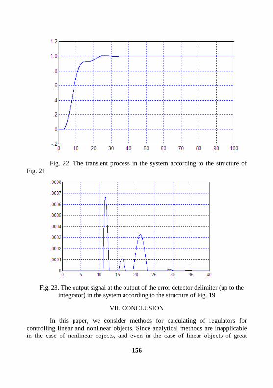
156
Fig. 22. The transient process in the system according to the structure of
Fig. 21
Fig. 23. The output signal at the output of the error detector delimiter (up to the
integrator) in the system according to the structure of Fig. 19
VII. CONCLUSION
In this paper, we consider methods for calculating of regulators for
controlling linear and nonlinear objects. Since analytical methods are inapplicable
in the case of nonlinear objects, and even in the case of linear objects of great

157
complexity, for example, with elements of pure delay, numerical optimization
methods are by now the only tools for solving these problems. The paper formulates
the basic requirements for the system and the mathematical apparatus and gives the
requirements for the physical feasibility of the model.
In this paper, we do not describe the control technique using local and
pseudo-local feedbacks, did not give detailed classification of adaptive systems and
authorial structures of adaptive systems, not considered systems with competitive
quality criteria. The papers of the authors published in the journal “Automatics &
Software Engineery”, in the proceedings of international conferences and in other
publication [1–10].
REFERENCES
[1] V. Zhmud., A. Liapidevskiy, E. Prokhorenko. “The design of the feedback systems by means of the modeling and optimization in the program vissim 5.0/6”. 2010. Proceedings of the IASTED International Conference on Modelling, Identification and Control, pp. 27–32.
[2] V. Zhmud, O. Yadrishnikov, A. Poloshchuk, A. Zavorin. “Modern key techologies in automatics: Structures and numerical optimization of regulators”. 2012. Proceedings - 2012 7th International Forum on Strategic Technology, IFOST 2012, paper 6357804.
[3] A.A.Voevoda, V.A.Zhmud, R.Y. Ishimtsev, V.M. Semibalamut. “The modeling tests of the new pid-regulators structures”. (2009) Proceedings of the IASTED International Conference on Applied Simulation and Modelling, ASM 2009, pp. 165–168.
[4] V. Zhmud, L. Dimitrov, O. Yadrishnikov. “Calculation of regulators for the problems of mechatronics by means of the numerical optimization method”. 2014. 12th International Conference on Actual Problems of Electronic Instrument Engineering, APEIE 2014 - Proceedings, paper 7040784, pp. 739–744.
[5] V. Zhmud, V. Semibalamut, A. Vostrikov. “Feedback systems with pseudo local loops”. 2015. Testing and Measurement: Techniques and Applications - Proceedings of the 2015 International Conference on Testing and Measurement: Techniques and Applications, TMTA. 2015, pp. 411–417.
[6] G.V. Sablina, I.V. Stazhilov, V.A. Zhmud. “Development of rotating pendulum stabilization algorithm and research of system properties with the controller”. 2016. 13th International Scientific-Technical Conference on Actual Problems of Electronic Instrument Engineering, APEIE 2016 - Proceedings, 3, paper 7807046, pp. 165–170.
[7] V. Zhmud, O. Yadrishnikov. “Numerical optimization of PID-regulators using the improper moving detector in cost function”. Proceedings of the 8-th International Forum on Strategic Technology 2013 (IFOST-2013), vol. II, 28 June – 1 July. Mongolian University of Science and Technology, Ulaanbaator, Mongolia. IEEE organized. 2013. P. 265–270. http://www.must.edu.mn/IFOST2013/
[8] V.A. Zhmud, A.A. Voevoda, R.Yu. Ishimtsev, V.M. Semibalamut. “New structures and methods of the scalar and multichannel regulators for non-

158
linear and/or delayed objects”. Proceedings of DST-RFBR-Sponsored Indo-Russian Joint Workshop on Computational Intelligence and Modern Heuristics in Automation and Robotics. S. V. National Institute of Technology, Surat – 395 007, Gujarat, India. 20th - 22nd September 2010. pp. 63–67.
[9] V. Zhmud, L.Dimitrov. “Designing of complete multi-channel PD-regulators by numerical optimization with simulation”. International Siberian conference on control and communications (SIBCON–2015): proc., Omsk, 21–23 May, 2015. – Omsk : IEEE, 2015. – Art. 129 (6 p.). ISBN 978-1-4799-7102-2. - DOI: 10.1109/SIBCON.2015.7147059.
[10] Zhmud V. A. Numerical Optimization of Locked Automatic Control
System in Software VisSim: New Structures and Methods: monograph / V. A.
Zhmud, L. V. Dimitrov, J. Nosek. - Novosibirsk: ZAO «KANT».
https://www.researchgate.net/publication/325012120_Numerical_Optimization_of_
Locked_Automatic_Control_System_in_Software_VisSim_New_Structures_and_
Methods

159
A Sub-Nyquist Spectrum Sensing Method Based on
Joint Recovery of Distributed MWCs
Jianxin Gai1, Xiao Teng,
2, Hailong Liu
3, Ziquan Tong
4
1,2,3,4Harbin University of Science and Technology (HUST)
Abstract—The recently proposed sub-Nyquist spectrum sensing
method based on Modulated Wideband Converter (MWC) can perform
sampling at a rate far below Nyquist frequency, which relieves sampling
pressure from wideband spectrum sensing. However, the success rate is far
from satisfactory due to the influences of shadow effect and so on. In this
paper, we present a distributed sub-Nyquist wideband spectrum sensing
method using joint recovery technique based on multiple MWCs. The
proposed sensing method can significantly improve the sensing performance
with the increase of node numbers by making full use of the joint sparse
structure across multiple signals and the diversity of sensing matrices.
Numerical experiments show that, compared with separate sensing method,
the proposed approach enhances the sensing performance in terms of success
rate, and it even can achieve a success when the separate sensing for each
MWC node fails.
Keywords—sub-Nyquist, distributed spectrum sensing, joint recovery,
sparse wideband signal
I. INTRODUCTION
Cognitive radio can achieve dynamic spectrum access, providing a new
solution for efficient utilization of spectrum resources. Fast spectrum sensing for
multiple channels in a wide frequency band is the premise and foundation for the
realization of cognitive radio [1]. However, wideband spectrum sensing faces the
pressure of high sampling rate [2-3]. The traditional method of spectrum estimation
requires that the sampling rate is not less than the Nyquist frequency, which is
undoubtedly a big problem for the radio signal with the bandwidth of GHz. The
development of analog-to-digital conversion hardware has a certain distance from
this requirement.
The recent emerging sub-Nyquist sampling approach named Modulated
Wideband Converter (MWC) provides a new acquisition and processing method for
sparse wideband signals. According to MWC, a sparse wideband signal can be
recovered perfectly from fewer non-adaptive measurements than the number

160
prescribed by the Nyquist theorem, provided the sensing matrix conforms to some
condition [4-5]. Compared with other sampling methods, MWC has the strength
that it can be implemented using existing devices with a lower-dimensional sensing
matrix, and the original signal can be perfectly recovered from samples at sub-
Nyquist rate. The MWC has tremendous potential impact because of the
longstanding, proven usefulness of spectral signal models in many engineering and
scientific applications [6]. Although MWC can be employed to realize sub-Nyquist
sampling on some condition, nevertheless the recovery performance of a single
MWC is still far from satisfactory. Furthermore, spectrum sensing for cognitive
radio requires multiple sensors to work in a cooperative manner to conquer the
problem that a single sensor cannot do. The distributed system is expected to
overcome the hidden terminal problem which is caused by the severe multipath
fading and the shadowing effect [7]. However, the distributed sub-Nyquist sampling
method based on MWC has not been researched sufficiently, and the existing
methods are incompetent for the distributed sensing model of multiple MWCs.
In this paper, we present a distributed sub-Nyquist spectrum sensing
method based on multiple MWCs. By exploiting the joint sparse structure across
the signals, we propose a highperformance joint recovery algorithm. Numerical
experiments demonstrate that, the proposed sensing approach based on joint
recovery can significantly enhance the spectrum sensing performance.
II. MWC OVERVIEW
MWC is a sub-Nyquist sampling method for sparse wideband signals. It adopts
spread-spectrum technique to deliberately alias all the subbands to the baseband,
which allows the low rate samples to incorporate complete information of the
original signal. As shown in Fig. 1, an MWC system has m parallel channels. The
input signal x ( t ) enters m channels simultaneously. In the ith channel x ( t ) is
mixed by Tp -period ( f p = 1 / Tp ) pseudo-random signal p (t ) .
After that, the signal is truncated in the frequency domain by an anti-aliasing
lowpass filter and then sampled at the rate f s = 1 / T which matches the cutoff 1 /
2T of the filter h ( t ) .
Applying classical Fourier analysis to MWC, the spectrum relation between the
output and the input can be derived as follows in f [ - f s / 2, fs / 2] ,

161
where cin are the Fourier series coefficietns of pi(t).
Fig. 1. Block diagram of the MWC system
From (1), it can be seen that the spectrum after being sampled by MWC
becomes a linear combination of fp-shifted copy of the original spectrum X ( f )
The shift interval f p is the frequency of p ( t ). If we consider Yi( e j 2π fT
) as the ith
entry of an m-dimensional column vector y(f) and X(f-nfp) as the nth entry of an L-
dimensional (L=2L0+1) column vector z(f) then (1) can be reformulated as follows,
where Φi,j= ci,j , and Φ is called sampling matrix with size m L and m
L .
Fig. 2 gives the illustration of the relation between the unknown spectrum
z( f ) and the output signal spectrum y( f ) . We can reconstruct X ( f ) easily as long
as the unknown vector z( f ) is obtained by a specific recovery method.

162
Fig. 2. Illustration of spectrum relations for input and output signals of
MWC
From (2), the relation between the unknown time sequence Z(n) and
measurements Y(n) can be developed by the inverse discrete time Fourier transform,
and we have
Y (n) = ΦZ(n) (3)
where Y (n) = [ y1 (n), y2 (n),..., ym (n)]T
and Z ( n ) [ z1 ( n ), z 2 ( n ), ..., z m ( n )]T
Therein, yi(n) is the time sequence acquired from the ith channel, and zi(n)
represents the unknown sequence corresponding to the ith unknown spectrum slice
in z(f) . Due to the condition m<L , both the matrix equations (2) and (3) are
underdetermined so that we generally can not obtain the unique solution directly by
inverse operations. Since the unknown z(f) or Z(n) has only few nonzero rows for
sparse wideband signals, we can obtain the unique sparsest solution. We should
first solve the support set of (3), and then perform the final recovery according to
pseudo-inversion. It is noted that in spectrum sensing application, complete
reconstruction of the signal is not needed, only the spectrum support is required to
further judge the unused spectrum slices.

163
III. DISTRIBUTED SUB-NYQUIST SPECTRUM SENSING
For cognitive radio, uncertain channel fading and random shadowing
would lead to varying signal strength at different receivers. Thus the distributed
spectrum sensing approaches were considered in [7] and [8]. Such methods may
significantly increase the reliability of the spectrum sensing process due to the
comprehensive consideration. Although sub-Nyquist sampling method based on
MWC has been proposed to sense the spectrum for cognitive radio, distributed
sensing method using multiple MWCs have not yet been studied sufficiently. For
distributed sub-Nyquist spectrum sensing, which is referred to as DSNSS
(Distributed Sub- Nyquist Spectrum Sensing) later, both the sampling approach and
recovery model differ from existing ones.
To achieve the potential strength of the distributed sensing, multiple MWC
nodes can be separately placed on several locations of interest to acquire the
different but correlated signals at sub-Nyquist rate of the same. Then the data
obtained from these sensors is sent to a fusion center in which the final information
is jointly recovered. Consider a distributed spectrum sensing system consisted of J
MWCs. The sensing model can be formulated as follows,
Yj = Φj Z j j 1, 2, ..., J (4)
where the sensing matrix Φj is of size m L with m L . Each unknown
matrix Z j with j 1, 2, ..., J consists of R sparse vectors, and all the matrices
share 2N nonzero rows. That is, the joint sparsity level
| ∪ supp(Z j ) | 2N
j 1,2,..., J where | S | represents the cardinality of the set S . Our task is to process the
J MMV (Multiple Measurement Vector) problems [9] for the information of
interest. For spectrum sensing, we do not need to recover each MMV problem
exactly. We only need to find the support set to make a decision. Intuitively, we can
solve (4) one by one through existing MMV recovery methods such as the
OMPMMV and MUSIC algorithm. However, this cannot benefit the total recovery
performance since the separate recovery process does not explore and take
advantage of more information of the multiple measurement matrices. In (4), the
unknown matrices have common nonzero rows, though the detailed entries of them
are different. So in the following section, we attempt to utilize the joint sparse
structure to seek a synchronous solving approach which can improve the sensing
performance.

164
IV. JOINT-SPARSE RECOVERY ALGORITHM
In this section we introduce a new algorithm by exploring the correlation
structures of the unknown matrices. We develop a method to recover the joint
support of the signals. In [10], we adopted MUSIC algorithms to perform support
recovery for a single MWC and achieved a good performance. Here, MUSIC can
also be considered. We generalize this algorithm to multiple-MWC scenario. For
MUSIC, in noisefree case the entries of support set decision Γj,l of the jth MWC is
zero for leven when there is a certain noise, this value is relatively small.
Hencre, if the l2 norm is used to synthesize the decision matrix Γj,l consisted of
each decision vectors into one row vector the value of the element value at the
index corresponding to the support set should also be relatively small. Conversely,
we can judge the common support set by sorting the value of the elements in this
vector. Table 1 gives the pseudo code of the DSNSS algorithm.
TABLE I. DSNSS Algorithm

165
In this algorithm, step 5 integrates the criteria of J support sets into a
unified criterion through l2 norm. Therefore, the final support set criterion vector
reflects the joint behavior of J-signals, which not only contains the diversity of
different sparsity coefficients, but also includes the diversity of the sensing matrix.
In addition, each support set criterion reflect the sparse structure of the
corresponding unknown matrix to a certain extent. So the criterion fusion is
equivalent to making full use of the sparse structure within the signal and the
common characteristics between the signals. It is because of the above advantages
that, in some cases, when the MWC isolation can not get the correct support set, the
DSNSS joint sensing algorithm can still achieve the successful recovery of the
support set.
V. EXPERIMENTS AND DISCUSSION
To evaluate the effectiveness of the proposed DSNSS spectrum sensing
method, in this section we experimentally compare the joint recovery performance
of DSNSS in terms of recovery rate with different numbers of MWCs, and show the
potential strength in spectrum sensing application. In these experiments, the sparse
wideband signals are generated by the following formula
x ( t ) E n Bn sinc( Bn ( t n )) cos(2 f n ( t n )) n (t )
where En, Bn, fn and n represent the energy coefficient, bandwidth, central
requency and time offset of the nth band for a multiband signal, and n ( t ) denotes
additive white Gaussian noise.
In order to simulate the actual sampling process of MWC, the analog
signal is represented by discretetime signal at Nyquist rate. In each experiment, the

166
following procedures are repeated for 500 times and the rate of success is computed
according to the percentage of successful recoveries.
The sign waveforms pi ( t ) are generated randomly with a uniform distribution.
The central frequencies fn are given randomly within the frequency interval
[-fNYQ/2, fNYQ/2].
The support sets are jointly recovered using the DSNSS algorithm or separately
recovered via MUSIC orOMPMMV.
If the estimated support set Ώ is the same with the original one Ω, we announce
a successful recovery. Moreover, if Ώ ⸧ Ω and Ф Ώ has full column rank, we also
regard the recovery as a success.
We examine the recovery performance of DSNSS under different numbers
of signals. Without loss of generality, we assume that there are J signals of interest,
and for each, we take the number of bands N = 6 as an example. The time offset τn
for the nth band of each signal is located randomly in the range of sampling
duration. The central frequencies of bands distribute in the span [-fNYQ/2, fNYQ/2]
randomly, where the Nyquist rate fNYQ = 10 GHz. The other parameters are fixed as:
En=1, 2, 3, Bn=50, 50, 50MHz. According to [4], the parameters for each
MWC are configured as follows: fs = fp = fNYQ /195 = 51.28 MHz; L 0 = 97, L =
2L0+1 = 195.
Since the performance enhancement of DSNSS is due to the use of more
information across multiple signals, if the number of signals increases, the recovery
performance is expected to be enhanced. To validate this, in this experiment, we
shift the signal number J 1, 2, 4, 8 and keep the other parameters unchanged.
As shown in Fig. 3, when the channel number m 25 , the recovery rate increases
with the rise of signal number J. For instance, when m 15 , the recovery rates are
22.0%, 61.5%, 85.0%, and 96.0% related to J = 1, 2, 4, 8, respectively. From the
perspective of necessary minimum channel number, we can notice that the
necessary channel number for exact recovery decreases with the increase of signal
number J. We would guess that the theoretical lower bound of channel number (m
2N ) will be achieved when J is large enough.

167
Fig. 3. Joint recovery rate curves of J signals with the shift of the number of
channels m under signal-to-noise ratio of 10dB
The distributed spectrum sensing and joint recovery method based on
DSNSS is expected to overcome severe fading and shadowing effect. To
demonstrate this advantage of DSNSS, we consider a setting in which there are 6
transmission bands (3 pairs) and nevertheless partial transmissions are shadowed so
as to the energy of corresponding bands becomes negligible at the specific receivers
consisted of MWCs. We assume that two MWCs are adopted to sense the spectrum
and for each the received bands are incomplete. The detailed setting is as the
following table.
TABLE II. Signal parameters at the two MWCs

168
Fig. 4. Comparison of average success rates between separate recoveries using
OMPMMV, DSNSS(J=1) and joint recovery using DSNSS(J=2)
Here because of the shadowing effect, the signal sensed by MWC #1 lacks band
#1, and the signal around MWC #2 is short of band #2. Thus for each MWC the
separate recovery result using MUSIC or OMPMMV fails to detect all the bands.
Fig. 4 demonstrates the average success rates of the separate recovery using
MUSIC and the joint recovery using DSNSS under SNR = 25dB. From this figure,
we can see that, neither of MWC #1 or #2 can obtain all the band information due
to the received incomplete information caused by the shadowing effect. In contrast,
the DSNSS joint recovery algorithm can successfully detect all the bands with
overwhelming probability when the number of channels is above 25. This shows
the strength of the proposed DSNSS method for the spectrum sensing application.
VI. CONCLUSIONS
In this paper, we present a distributed sub-Nyquist spectrum sensing method based on multiple MWCs and a high-performance joint recovery algorithm. The proposed algorithm can improve the support recovery performance by using the joint sparse structure across multiple signals. Numerical experiments demonstrate that the joint recovery algorithm for multiple MWCs can significantly outperform the recovery approach for a single MWC in terms of sensing success rate. The success rate of joint recovery increases as the signal number rises, and the necessary number of hardware channels to achieve the same recovery rate deceases with the increase of the signal number. The proposed method can mitigate fading and shadowing effect owing to the cooperation between multiple nodes. Future works may include exploring a more efficient joint recovery algorithm for the distributed sub-Nyquist spectrum sensing problem.
ACKNOWLEDGEMENTS

169
This work was supported in part by the National Natural Science
Foundation of China (NSFC) under grants 61501150, and the Youth Science
Foundation of Heilongjiang Province under grants QC2014C074.
REFERENCES
[1] Kakalou I., Papadopoulou D., Xifilidis T., “A survey on spectrum
sensing algorithms for cognitive radio networks”, 2018 7th International
Conference on Modern Circuits and Systems Technologies (MOCAST), pp.1–4,
2018.
[2] Mashhour M. and Hussein A. “Sub-Nyquist wideband spectrum
sensing based on random demodulation in cognitive radio”, 2017 12th International
Conference on Computer Engineering and Systems (ICCES), pp.712–716, 2017.
[3] Qi P., Li Z., Li H., and Xiong T., “Blind Sub-Nyquist Spectrum
Sensing With Modulated Wideband Converter”, IEEE Transactions on Vehicular
Technology, vol.67, no.5, pp. 4278 - 4288, 2018.
[4] Mishali M., Eldar Y. C., “From theory to practice: sub-Nyquist
sampling of sparse wideband analog signals”, IEEE Journal of Selected Topics in
Signal Processing, vol. 4, no. 2, pp. 375–391, 2010.
[5] Adams D, Eldar Y C and Murmann B., “A mixer front end for a
four channel modulated wideband converter with 62-dB blocker rejection”. IEEE
Journal of Solid-State Circuits, vol.20, no.5, pp.1286-1294, 2017.
[6] Lexa, M. A., Davies M. E., Thompson J. S., “Reconciling
Compressive Sampling Systems for Spectrally Sparse Continuous-Time Signals”,
IEEE Transactions on Signal Processing, vol. 60, no. 1, pp. 155–171, 2012.
[7] Timalsina S. K., Moh S., and Lee J., “Cooperative Approaches to
Spectrum Sensing and Sharing for Cognitive Radio Networks: A Comparative
Study”, JNIT: Journal of Next Generation Information Technology, vol. 2, no. 4,
pp. 10–23, 2011.
[8] Rasheed T., Rashdi A., Akhtar A. N., “Cooperative spectrum
sensing using fuzzy logic for cognitive radio network”, 2018 Advances in Science
and Engineering Technology International Conferences (ASET), pp.1–6, 2018.
[9] Cotter F. S., Rao D. B., Engan K, “Sparse solutions to linear
inverse problems with multiple measurement vectors”, IEEE Transactions on
Signal Processing, vol. 53, no. 7, pp. 2477–2488, 2005.
[10] Gai J., Fu P., Fu N., and Liu B. “Sub-Nyquist sampling
reconstruction algorithm based on SVD and MUSIC”vol. 33, no. 9, pp. 2073-2079,
2012.