International trade and social connectedness

Journal of International Economics 129 (2021) 103418

Contents lists available at ScienceDirect

Journal of International Economics

j ourna l homepage: www.e lsev ie r .com/ locate / j i e

International trade and social connectedness

Michael Bailey a, Abhinav Gupta b, Sebastian Hillenbrand b, Theresa Kuchler b,Robert Richmond b,⁎, Johannes Stroebel ba Facebook, Inc, United States of Americab Stern School of Business, New York University, United States of America

a r t i c l e i n f o

⁎ Corresponding author.E-mail addresses:[email protected] (M. Bailey), agu

[email protected] (R. Richmond), johannes.stroe1 Prominent contributions that have explored the re

Rogoff (2000), Eaton and Kortum (2002), and Hortaçsu

https://doi.org/10.1016/j.jinteco.2020.1034180022-1996/© 2020 Elsevier B.V. All rights reserved.

a b s t r a c t

Article history:Received 11 September 2020Received in revised form 23 December 2020Accepted 23 December 2020Available online 29 December 2020

Dataset link: https://data.mendeley.com/datasets/7wddm84w9r/1

We use de-identified data from Facebook to construct a new and publicly available measure ofthe pairwise social connectedness between 170 countries and 332 European regions. We findthat two countries trade more when they are more socially connected, especially for goodswhere information frictions may be large. The social connections that predict trade in specificproducts are those between the regions where the product is produced in the exporting coun-try and the regions where it is used in the importing country. Once we control for social con-nectedness, the estimated effects of geographic distance and country borders on trade declinesubstantially.

© 2020 Elsevier B.V. All rights reserved.
JEL codes:F1F5F6
Keywords:International tradeSocial connectednessInformation frictionsBorder effects

The propensity for residents of different countries to be connected to one another varies enormously. For example, aU.S.-based Facebook user is 65% more likely to be friends with a given Facebook user living in Germany than with agiven Facebook user living in France. Such differences in bilateral social connectedness play an important role in many nar-ratives of economic and political interactions between countries. For example, beginning with Tinbergen (1962), re-searchers have explored the determinants of international trade using gravity models that relate trade between countriesto various measures of the relationship between those countries.1 These models have had substantial empirical success,but their economic underpinnings—and especially the mechanisms behind the large estimated negative effect of physicaldistance on trade—have remained elusive. One prominent explanation is that geographic closeness proxies for social con-nections between individuals, which can help facilitate trade. While such a mechanism is intuitively appealing, the absenceof comprehensive data on social connections across regions and countries has limited researchers' ability to provide evi-dence in favor of this interpretation.

[email protected] (A. Gupta), [email protected] (S. Hillenbrand), [email protected] (T. Kuchler),[email protected] (J. Stroebel).lationship between geography and trade include Leamer and Levinsohn (1995), Trefler (1995), Obstfeld andet al., (2009).

http://crossmark.crossref.org/dialog/?doi=10.1016/j.jinteco.2020.103418&domain=pdf

https://data.mendeley.com/datasets/7wddm84w9r/1

https://data.mendeley.com/datasets/7wddm84w9r/1

https://doi.org/10.1016/j.jinteco.2020.103418

[email protected]

https://doi.org/10.1016/j.jinteco.2020.103418

http://www.sciencedirect.com/science/journal/

www.elsevier.com/locate/jie

M. Bailey, A. Gupta, S. Hillenbrand et al. Journal of International Economics 129 (2021) 103418

In this paper, we introduce a new measure of the pairwise social connectedness between 170 countries and 332 European re-gions, and show that much of the variation in global trade can indeed be explained by patterns of social connectedness. We alsofind support for mechanisms proposed by theoretical models in which social connectedness facilitates trade by reducing informa-tion frictions.2 By exploiting the granular nature of our social connectedness measure and detailed data on the geography of pro-duction, we are able to further understand the impact of social connectedness on trade flows. Specifically, we show that it is thesocial connections between the regions where a good is produced in the exporting country and those regions where it is used inthe importing country that predict trade in that good. Once we control for social connectedness, the estimated effects of geo-graphic distance and country borders on trade decline substantially.

Our measure of social connectedness is based on a de-identified snapshot of all friendship links on Facebook, the world's larg-est online networking site with more than 2.7 billion active users around the globe. Our Social Connectedness Index between pairsof regions corresponds to the relative probability of a friendship link between Facebook users in the two regions. We constructthis pairwise measure of social connectedness for 170 countries and 332 European regions. To facilitate further research on therelationship between social connectedness and trade flows, we have made the Social Connectedness Index publicly available toother researchers.3

When relating the Social Connectedness Index to trade flows, we do not interpret our findings as evidence that Facebook linksdirectly cause or facilitate trade. Instead, we interpret our measure of social connectedness as providing a high-quality proxy forexisting trade-facilitating relationships across countries and regions. The ability of our data to capture these relationships at a geo-graphically disaggregated level is the result of Facebook's scale, the relative representativeness of its user body, and the fact thatpeople primarily use Facebook to interact with real-world friends and acquaintances. Throughout the paper, we present a numberof results that mitigate concerns that our findings are the result of omitted country-level variables or reverse causality wherebytrade flows lead to more underlying friendships.

We first describe the rich patterns of social connectedness observed in our data. About half the variation in social connected-ness between countries is explained by geographic distance. Quantitatively, a 10% increase in the distance between two countriesis associated with a 12%–16% decline in their social connectedness. Migration patterns and colonial history further influence theprobability of present-day friendship links across country pairs. We also find stronger social connections between countries thatshare a common language, as well as between countries that are similar in terms of economic development, religious beliefs, andthe genetic make-up of their populations. Within Europe, common language and common history shape the social connectednessbetween regions over and above distance and common nationality. Beyond these systematic patterns, our measure of social con-nectedness is also affected by idiosyncratic factors that are specific to particular country and region pairs.

Next, we document that patterns of social connectedness explain a substantial part of the variation in international tradeflows. When we introduce social connectedness into a standard gravity model of country-level goods trade, we find that socialconnectedness and geographic distance explain similar shares of the cross-sectional variation in trade flows. The elasticity oftrade in goods with respect to social connectedness is 0.28 in specifications that also control for geographic distance. This impliesthat, all else equal, trade between the U.S. and Germany should be 18% higher than trade between the U.S. and France, since theU.S. is 65% more connected to Germany than it is to France. Controlling for social connectedness reduces the distance elasticity oftrade from about −1 to roughly −0.70. This is a substantial decline that does not occur when controlling for other gravity vari-ables such as common language or common colonial origins. Social connectedness as measured by today's Facebook links stronglyexplains trade flows at least since the 1980s, demonstrating that the underlying trade-facilitating relationships across countriesare very stable over time. The combined evidence suggests that social connectedness is an important determinant of tradeflows, and highlights that the relationship between geographic distance and trade in the prior literature might partially capturethis role of social connectedness.

We then explore possible explanations for the observed relationship between trade flows and social connectedness. In partic-ular, the literature has proposed that social links can facilitate trade by alleviating a number of informal trade barriers, includingcontract enforcement frictions and search costs due to information frictions (see Chaney, 2016, for a review). We provide evi-dence suggesting that social links as measured through the Social Connectedness Index help alleviate information frictions whilethey do not appear to significantly mitigate contract enforcement frictions.

We first study how the elasticity of trade with respect to social connectedness varies for trade in different products. In partic-ular, Rauch (1999) and Rauch and Trindade (2002) suggest that information frictions are largest for products that are not tradedon organized exchanges. Consistent with the idea that social connections can help to mitigate such information frictions, we showthat the elasticity of trade to social connectedness is particularly large for these non-exchange-traded goods. To understandwhether social connectedness can mitigate contract enforcement frictions, we also study how the elasticity varies with measuresof the rule of law in the importing and exporting countries. This analysis is motivated by a literature that shows that weak rule oflaw reduces trade due to difficulties with the enforcement of contracts (e.g., Anderson and Marcouiller, 2002). In these

2 Papers which study the role of information frictions in international trade include, Jensen (2007); Aker (2010); Allen (2014); Chaney (2014); Simonovska andWaugh (2014); Startz (2016); Steinwender (2018).

3 This new and comprehensive measure of international social connectedness can be downloaded at https://data.humdata.org/dataset/social-connectedness-index.See Bailey et al. (2018a, 2020a) for a description of a related data setmeasuring the social connectedness betweenU.S. counties, and between zip codes in theNewYorkmetro area. See Bali et al. (2018), Hirshleifer et al. (2019), Rehbein et al. (2020), Kuchler et al. (2020a, 2020b), Bailey et al. (2020b), andWilson (2019) for recent uses ofthe U.S. Social Connectedness Index in economics and finance research.

2

https://data.humdata.org/dataset/social-connectedness-index


regressions, we find little variation in the elasticity across countries with different levels of rule of law, suggesting that the pri-mary channel behind the observed aggregate relationships is the reduction of information frictions.

After documenting how social connectedness relates to trade at the country level, we use our granular measure of social con-nectedness across sub-national European regions to further understand the mechanism behind the observed relationships. Our re-sults in that section provide new evidence on the interaction of trade flows, the spatial distribution of production, and thestructure of social networks. Our findings also help us rule out country-level omitted variables or reverse causality as alternativeinterpretations of the observed aggregate relationship between social connectedness and trade.

Our approach builds on a literature that documents that firms and individuals working at those firms are central to facilitatinginternational goods trade.4 Based on this insight, we construct product-specific measures of the social connectedness betweencountries, which overweight the connectedness between those regions where the goods are produced in the exporting countryand those regions where the goods are used in the importing country. This measure contrasts with our baseline measure of socialconnectedness between two countries, which corresponds to the population-weighted average connectedness between all regionsin the countries. As an example, more than 80% of Italian exports of non-metallic mineral products to Greece are used as inputs inthe Greek construction sector. Our proposed measure of social connectedness relevant for exporting non-metallic mineral prod-ucts from Italy to Greece thus overweights the observed connectedness between the regions that produce non-metallic mineralproducts in Italy (primarily the Piedmont region around Torino) and the regions with significant construction employment inGreece (e.g., the Attica region around Athens).

We then regress product-level trade between countries on both measures of social connectedness. When controlling for theproduct-specific measure of social connectedness, the population-weighted measure has no further predictive power for tradeat the product-level. This remains true after controlling for product-specific measures of distance. This evidence suggests that itreally is the social connectedness between the regions where a good is produced and the regions where it is used that mattersfor trade in that good. We also find that the elasticity of trade to the product-specific measures of social connectedness is unaf-fected by the inclusion of country pair fixed effects, which absorb all country-level determinants of trade. This finding dramaticallyreduces the scope for omitted variables such as common preferences to explain the observed relationships between social con-nectedness and trade.

Our analysis of the effects on trade of product-specific social connectedness between countries also allows us to rule out thepresence of a quantitatively large reverse causality from trade to our measure of connectedness. If trade did in fact cause substan-tial social connections, the various product-specific measures of social connectedness between two countries should be systemat-ically larger than these countries' measures of population-weighted social connectedness. For instance, in the example above, wewould expect the Piedmont region in Italy and the Attica region in Greece to be disproportionately more connected than a ran-dom pair of regions in the two countries, as a result of the connections formed from trading non-metallic mineral products. Incontrast with this prediction, we find that the regions that are most important for the trade in a given product are equally likelyto be more or less connected than two random regions across a country pair.

In the final part of the paper, we study the relationship between regional social connectedness and sub-national goods trade.We use rail-freight flows between regions in the European Union as our measure of trade flows. This analysis allows us to exam-ine the determinants of the border effect, the empirical regularity that, conditional on the distance between two regions, trade ismuch larger between regions of same country (see McCallum, 1995; Anderson and Van Wincoop, 2003; Chen, 2004). Consistentwith existing estimates of the border effect, we find that, all else equal, trade within countries is seven to nine times as large astrade between countries. This is true despite the fact that the European Union is a common market with few formal barriers tocross-country trade. When we control for the social connections between regions, the estimated border effect drops by between75% and 90% across various specifications. This suggests that much of the effect of borders on trade may be the result of the factthat social connections fall at borders.

The rest of the paper is organized as follows. Section 1 presents our new measure of international social connectedness andexplores its determinants. Section 2 describes the relationship between international trade flows and social connectedness.Section 3 studies the mechanism through which social connectedness influences trade patterns, focusing on heterogeneities acrossproducts and countries. In Section 4, we present results using our product-specific measures of social connectedness and explorepatterns in regional trade within Europe.

1. Measuring international social connectedness

We construct our measure of the social connectedness between countries and European regions using de-identified adminis-trative data from Facebook, a global online social networking service. Facebook was created in 2004, and, by the second quarter ofof 2020, had 2.7 billion monthly active users globally. Of these monthly active users, 256 million were based in the U.S. andCanada, 410 million in Europe, 1.14 billion in the Asia-Pacific region, and 892 million in the rest of the world. With the exceptionof a few countries where social media services including Facebook are banned—most notably China, Iran, and North Korea—Facebook has a non-trivial footprint in essentially all countries around the world.

We work with a de-identified snapshot of all active Facebook users from August 2020. For these users, we observe their coun-try of location, as well as the set of other Facebook users that they are connected to. For users in Europe, we also observe their

4 Papers that study the importance of firms in trade includeMelitz (2003), Bernard et al. (2003), Bernard et al. (2007), Chaney (2008), Helpman et al. (2008), Melitand Ottaviano (2008), Chaney (2018), and Bernard et al. (2012).

3

z


region of location at the NUTS2 (Nomenclature of Territorial Units for Statistics level 2 regions) level, similar to Bailey et al.(2020c). These NUTS2 regions include between 800,000 and 3,000,000 individuals, and are defined for European Union members,European Union candidates, and European Free Trade Association members. They are generally based on existing subnational ad-ministrative borders. For example, in Italy the NUTS2 geographies correspond to the 21 “regions”, while in the Netherlands theycorrespond to the 12 “provinces”; smaller countries in Europe, such as Latvia and Malta, are represented by a single NUTS2 region.Location in a country or region is assigned based on users' information and activity on Facebook, including the stated city on theirFacebook profile, and device and connection information.

To compare the intensity of social connectedness between locations with varying populations and varying Facebook usagerates, we construct our Social Connectedness Index, SCIi,j, as the total number of connections between individuals in location iand individuals in location j, divided by the product of the number of Facebook users in those locations, as in Eq. 1:

5 TheIsrael, Nnumber

6 Diffhad accworry t

SCIi,j ¼FB_Connectionsi,j

FB_Usersi � FB_Usersjð1Þ

For both countries and regions, we rescale this number to have a minimum value of 1, and a maximum value of 1,000,000. TheSocial Connectedness Index therefore measures the relative probability of a Facebook friendship link between a given Facebook userin location i and a given user in location j. Overall, we will work with information on the pairwise social connectedness between170 countries, for a total of 170 × 169 = 28,730 country-pair combinations. At the NUTS2 level, we observe the social connect-edness between 332 × 331 = 109,892 pairs of European regions.5

1.1. Interpreting the social connectedness index

Two important questions arise when interpreting SCIi,j as a proxy for potentially trade-facilitating relations between countriesor regions: whether Facebook friendships correspond to real-world friendship links of Facebook users, and whether Facebookusers are representative of the countries' or regions' populations.

On the first issue, we believe that Facebook friendships provide a reasonable proxy for real world friendship networks. For theUnited States, Duggan et al. (2015) have shown that Facebook friendship patterns correspond closely to real-world friendship net-works. While similar studies do not exist for most other countries, we believe that there are a number of reasons to think that weare also capturing good representations of real-world social networks of Facebook users outside of the United States. For example,establishing a connection on Facebook requires the consent of both individuals, and there is an upper limit of 5,000 on the num-ber of connections a person can have. As a result, networks formed on Facebook will more closely resemble real-world social net-works than those on other online platforms, such as Twitter, where uni-directional links to non-acquaintances, such as celebrities,are common. Consistent with this conclusion, our prior work with micro-data from Facebook has found that many economic de-cisions, such as whether to buy a house or which phone to purchase, are influenced by related decisions of a person's Facebookfriends (Bailey et al., 2018b, 2019a, 2019b).

On the second issue, it is likely that the representativeness of Facebook users will differ across locations. While Duggan et al.(2016) have shown that U.S. Facebook users are quite representative of the U.S. population, this is unlikely to be the case every-where. For example, in countries with relatively low internet penetrations, those individuals with access to the internet are likelyto be a non-representative subset of the overall populations. To the extent that having internet access and having friends abroadare positively correlated, our measure would then overstate the international linkages of the average resident in countries withlow internet usage.6 In our analysis, we account for such heterogeneities in the average connectedness of each location by includ-ing fixed effects for locations i and j in all specifications. This approach allows us to explore connectedness between locationsi and j, holding fixed the average propensity in each location of having Facebook friends in different places.

In the end, while no measure of social connectedness is perfect, we believe that our Social Connectedness Index, which is basedon hundreds of billions of Facebook friendship links from 2.7 billion Facebook users, provides a valuable large-scale measure ofthe geographic distribution of social networks. Indeed, it is hard to imagine an alternative measure that would allow us to mea-sure social connections at this scale and scope. We hope that the easy accessibility of our Social Connectedness Index will facilitatemore research on the role of social connectedness in economics and across the social sciences.

1.2. Determinants of social connectedness

We next explore a number of factors that help explain the observed patterns of social connectedness across locations. Wesummarize our central findings in the main body of the paper and present a more extensive analysis in Appendix A.

We begin by exploring a few case studies that highlight how social connectedness varies across specific countries and regions.

publicly available Social Connectedness Index data does not include information for a number of countries, such as Afghanistan, China, Cuba, Eritrea, Iran, Iraqorth Korea, Russia, Somalia, Sudan, Syria, Tajikistan, Turkmenistan, Venezuela, Western Sahara, and Yemen. In addition, we are missing gravity variables forof countries that are included in the SCI data (e.g., Montenegro, Serbia, and Kosovo).erential online access is less of an issue across our European regions. Indeed, statistics fromEurostat show that in 2019, 90% of households in the EuropeanUnioness to the internet. However, Facebook usage rates conditional on internet access can still vary in systematic ways across these regions. As a result, one mighhat Facebook users in regions with lower Facebook penetrations are connected to other regions at rates that are not representative of the full populations.

4

,a

t


Panel A of Fig. 1 shows the social connectedness of Portugal to other countries around the world. Darker colors correspond tohigher connectedness. Portugal has the strongest links to geographically close countries in Western Europe. Portugal's interna-tional connections also highlight the role of colonial history and language in shaping present-day social connectedness. The coun-try is strongly connected to its former (Portuguese-speaking) colonies Brazil, Angola, Guinea-Bissau, and Mozambique. WithinEurope, Portugal is most strongly connected to Luxembourg. These connections, which are stronger than the connections toPortugal's neighbor Spain, are likely related to the fact that 15%–20% of Luxembourg's population is of Portuguese origin, followinglarge-scale migration from Portugal to Luxembourg as part of a guest worker program in the 1960s. This finding suggests that pastmigration movements continue to influence social connections today.

In Appendix A, we explore the determinants of international social connectedness more systematically. We find that a 10% in-crease in the distance between two countries is associated with a 10%–15% decline in their social connectedness. Geographic dis-tance explains about 50% of the variation in social connectedness that remains after accounting for country fixed effects.Consistent with our findings for Portugal, international migration patterns and colonial history strongly influence the probabilityof present-day friendship links across all country pairs. We also find more social connections between countries sharing a com-mon language, as well as between countries that are similar in terms of economic development, religious beliefs, and the geneticmake-up of their populations. However, while about 70% of the variation in social connectedness across country pairs can be ex-plained by distance, language, and other systematic factors, our Social Connectedness Index also captures a wide variety of idiosyn-cratic forces that can shape the social connections between two countries. For example, citizens of Denmark and Australia are 75%more connected than would be predicted purely by the observable factors described above. These strong social connectionsbetween Denmark and Australia are likely the result of the 2004 marriage of the Danish Crown Prince Frederik toAustralian-born Mary Donaldson. This marriage led to heightened mutual interest between Danish and Australian citizens, andhas substantially increased tourism between the two countries.7 Examples such as this highlight the power of our approach tomeasuring social connectedness over and above competing approaches that proxy for social connectedness using a variety ofother gravity variables.

Panel B of Fig. 1 shows the connectedness of the Algarve region in southern Portugal to other regions within Europe. Thestrongest social links are to other regions in Portugal. Indeed, the Algarve region is much more strongly connected to the Norteregion in the very north of Portugal than it is to the Andalusia region, its neighbor just across the border in Spain. The Algarve'sconnections to other European regions show some of the same patterns seen for Portugal as a whole, such as the strong connec-tions to Luxembourg. However, additional nuances are visible at the regional level. At the country level, Portugal showed strongconnections to France. When exploring regional social connectedness, we find that connections from Algarve are particularlystrong to Southern France and Corsica, which has a substantial number of Portuguese immigrants. The Algarve also has strongconnections to much of Western Europe, from where it attracts many tourists each year.

The forces highlighted in Panel B of Fig. 1 also show up in more systematic analyses. Indeed, Bailey et al. (2020c) show thatsocial connectedness within Europe varies with patterns of migration, political borders, geographic distance, language, and otherdemographics. The elasticity of social connectedness with respect to distance across European regions is −1.3, similar to compa-rable elasticities across countries. Social connectedness drops off sharply at country borders, even after controlling for distance:depending on the country, the probability of friendship between two individuals living in the same country is five to eighteentimes as large as the probability of friendship across two individuals living in different countries. In addition, regions that aremore similar along demographic measures such as language, religion, education, and age are more socially connected. Interest-ingly, the relationship between political borders and connectedness can persist many decades after boundaries change. For exam-ple, Bailey et al. (2020c) finds higher social connectedness across regions that were originally part of the Austro-Hungarianempire, even after controlling for a host of other determinants of present-day social connectedness.

2. Country-level trade and social connectedness

We now turn to understanding the relationship between social connectedness and trade at the country level. We first docu-ment that trade flows are increasing in social connectedness and show that these effects are larger for goods where informationfrictions may be important, suggesting that social connections may facilitate trade by reducing these frictions.

We measure country-level trade flows using bilateral goods trade data from CEPII (Gaulier and Zignago, 2010). In our baselineanalysis, we explore data from 2017, though our results are robust to using trade data from earlier or later years. The raw tradedata is disaggregated at the 6-digit HS96 code level, and contains information on 4,914 product categories. For our first analysis,we aggregate the product-level trade data into bilateral trade flows between country pairs. When merged with social connected-ness and gravity data, we have information on 27,060 country pairs.8 To understand the relationship between social connected-ness and trade flows, we follow the literature to estimate the following gravity regression:

7 Thethemarto Denm

8 ThisSwazila

Xi,j ¼ exp β1 log SCIi,j� �

þ β2 log Distancei,j� �

þ β3Gi,j þ δi þ δjh i

⋅εi,j ð2Þ

Australian Department of Foreign Affairs and Trade notes on its country brief on Denmark that “Australia's profile in Denmark, and vice-versa, was boosted byriage inMay 2004 of Australian-bornMaryDonaldson to Denmark's Crown Prince Frederik” and the press reported an increase of 30% in tourism fromAustraliaark in 2004.corresponds to pairwise trade data from 165 countries. Relative to the analysis in Appendix A, we lose Botswana, Lesotho, Luxembourg, Namibia, and

nd, for which we have data on social connectedness, but no data on trade.

5

Fig. 1. Social Connectedness of Portugal and Algarve Region. Note: Figure shows a heat map of the social connectedness of Portugal to other countries (PanelA) and of the Algarve region in Portugal to other European regions (Panel B). For each location, the colors highlight connections of the focal location, given inred. The lightest color corresponds to the 20th percentile of the connectedness across country pairs that include Portugal in Panel A and region pairs that includeAlgarve in Panel B; darker colors correspond to closer connections.


6

9 Ourzero traestimat


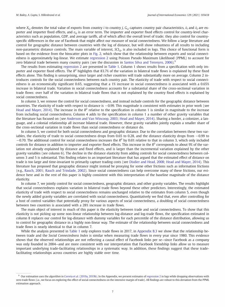
where Xi,j denotes the total value of exports from country i to country j, Gi,j captures country pair characteristics, δi and δj are ex-porter and importer fixed effects, and εi,j is an error term. The importer and exporter fixed effects control for country-level char-acteristics such as population, GDP, and average tariffs, all of which affect the overall level of trade; they also control for country-specific differences in the use of Facebook that might affect our measure of social connectedness. We follow a large literature andcontrol for geographic distance between countries with the log of distance, but will show robustness of all results to includingnon-parametric distance controls. The main variable of interest, SCIi,j, is also included in logs. This choice of functional form isbased on the evidence from the binscatter plots in Fig. 2, which show that the relationship between exports and social connect-edness is approximately log-linear. We estimate regression 2 using Poisson Pseudo Maximum Likelihood (PPML) to account forzero bilateral trade between many country pairs (see the discussion in Santos Silva and Tenreyro, 2006).9

The results from estimating regression 2 are presented in Table 1. Column 1 shows results from a specification with only im-porter and exporter fixed effects. The R2 highlights that 83.7% of the variation in bilateral trade flows is explained by these fixedeffects alone. This finding is unsurprising, since larger and richer countries will trade substantially more on average. Column 2 in-troduces controls for the social connectedness between each country pair. The elasticity of trade with respect to social connect-edness is an economically significant 0.65, suggesting that a 1% increase in social connectedness is associated with a 0.65%increase in bilateral trade. Variation in social connectedness accounts for a substantial share of the cross-sectional variation intrade flows: over half of the variation in bilateral trade flows that is not explained by the country fixed effects is explained bysocial connectedness.

In column 3, we remove the control for social connectedness, and instead include controls for the geographic distance betweencountries. The elasticity of trade with respect to distance is −0.99. This magnitude is consistent with estimates in prior work (seeHead and Mayer, 2014). The increase in the R2 relative to the specification in column 1 is similar in magnitude to the increasefrom including social connectedness. Column 4 adds to the specification in column 1 a number of other gravity variables thatthe literature has focused on (see Anderson and Van Wincoop, 2003; Head and Mayer, 2014). Sharing a border, a colonizer, a lan-guage, and a colonial relationship all increase bilateral trade. However, these gravity variables jointly explain a smaller share ofthe cross-sectional variation in trade flows than social connectedness or distance do.

In column 5, we control for both social connectedness and geographic distance. Due to the correlation between these two var-iables, the elasticity of trade to social connectedness drops from 0.65 to 0.28, and the distance elasticity drops from −0.99 to−0.70. The additional control for social connectedness increases the R2 by 0.6% relative to that in column 3, which only includedcontrols for distance in addition to importer and exporter fixed effects. This increase in the R2 corresponds to about 9% of the var-iation not already explained by distance and fixed effects, and is larger than the incremental variation explained by the othergravity variables (see column 6). The decline in the distance elasticity from adding controls for social connectedness between col-umns 3 and 5 is substantial. This finding relates to an important literature that has argued that the estimated effect of distance ontrade is too large and time-invariant to primarily capture trading costs (see Disdier and Head, 2008; Head and Mayer, 2014). Thisliterature has proposed that geographic distance might instead be proxying for some other frictions such as information frictions(e.g., Rauch, 2001; Rauch and Trindade, 2002). Since social connectedness can help overcome many of these frictions, our evi-dence here and in the rest of this paper is highly consistent with this interpretation of the baseline magnitude of the distanceelasticity.

In column 7, we jointly control for social connectedness, geographic distance, and other gravity variables. The results highlightthat social connectedness explains variation in bilateral trade flows beyond these other predictors. Interestingly, the estimatedelasticity of trade with respect to social connectedness remains unchanged relative to the estimates from column 5, even thoughthe newly added gravity variables are correlated with social connectedness. Quantitatively we find that, even after controlling fora host of control variables that potentially proxy for various aspects of social connectedness, a doubling of social connectednessbetween two countries is associated with a 28% increase in trade flows.

The main object of interest in much of this paper is the elasticity between trade and social connectedness. To show that thiselasticity is not picking up some non-linear relationship between log-distance and log-trade flows, the specification estimated incolumn 8 replaces our control for log-distance with dummy variables for each percentile of the distance distribution, allowing usto control for geographic distance in a highly non-linear way. The estimate of the relationship between social connectedness andtrade flows is nearly identical to that in column 7.

While the analysis presented in Table 1 only explores trade flows in 2017, in Appendix B.3 we show that the relationship be-tween trade and the Social Connectedness Index is similar when measuring trade flows in every year since 1980. This evidenceshows that the observed relationships are not reflecting a causal effect of Facebook links per se—since Facebook as a companywas only founded in 2004—and are more consistent with our interpretation that Facebook friendship links allow us to measureimportant underlying trade-facilitating relationships in a systematic way. In addition, these findings suggest that these trade-facilitating relationships across countries are highly stable over time.

estimation uses the algorithm in Correia et al. (2019a, 2019b). In the Appendix, we present estimates of regression 2 in logs while dropping observations withde flows (i.e., we focus on exploring the effect of social connectedness on the intensivemargin of trade). All findings are robust to this deviation from the PPMLion approach.

7

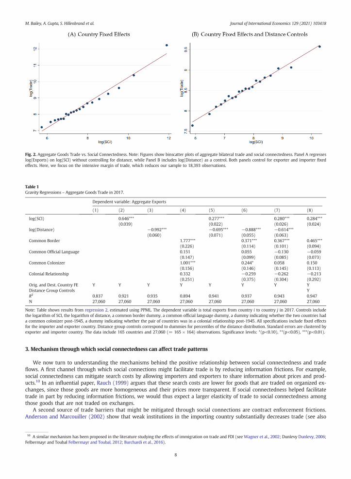
Fig. 2. Aggregate Goods Trade vs. Social Connectedness. Note: Figures show binscatter plots of aggregate bilateral trade and social connectedness. Panel A regresseslog(Exports) on log(SCI) without controlling for distance, while Panel B includes log(Distance) as a control. Both panels control for exporter and importer fixedeffects. Here, we focus on the intensive margin of trade, which reduces our sample to 18,393 observations.

Table 1Gravity Regressions – Aggregate Goods Trade in 2017.

Dependent variable: Aggregate Exports

(1) (2) (3) (4) (5) (6) (7) (8)

log(SCI) 0.646*** 0.277*** 0.280*** 0.284***(0.039) (0.022) (0.026) (0.024)

log(Distance) −0.992*** −0.695*** −0.888*** −0.614***(0.060) (0.071) (0.055) (0.063)

Common Border 1.777*** 0.371*** 0.367*** 0.465***(0.226) (0.114) (0.101) (0.094)

Common Official Language 0.151 0.055 −0.130 −0.059(0.147) (0.099) (0.085) (0.073)

Common Colonizer 1.001*** 0.244* 0.058 0.150(0.156) (0.146) (0.145) (0.113)

Colonial Relationship 0.332 −0.259 −0.262 −0.213(0.251) (0.375) (0.304) (0.292)

Orig. and Dest. Country FE Y Y Y Y Y Y Y YDistance Group Controls YR2 0.837 0.921 0.935 0.894 0.941 0.937 0.943 0.947N 27,060 27,060 27,060 27,060 27,060 27,060 27,060 27,060

Note: Table shows results from regression 2, estimated using PPML. The dependent variable is total exports from country i to country j in 2017. Controls includethe logarithm of SCI, the logarithm of distance, a common border dummy, a common official language dummy, a dummy indicating whether the two countries hada common colonizer post-1945, a dummy indicating whether the pair of countries was in a colonial relationship post-1945. All specifications include fixed effectsfor the importer and exporter country. Distance group controls correspond to dummies for percentiles of the distance distribution. Standard errors are clustered byexporter and importer country. The data include 165 countries and 27,060 (= 165 × 164) observations. Significance levels: *(p<0.10), **(p<0.05), ***(p<0.01).


3. Mechanism through which social connectedness can affect trade patterns

We now turn to understanding the mechanisms behind the positive relationship between social connectedness and tradeflows. A first channel through which social connections might facilitate trade is by reducing information frictions. For example,social connectedness can mitigate search costs by allowing importers and exporters to share information about prices and prod-ucts.10 In an influential paper, Rauch (1999) argues that these search costs are lower for goods that are traded on organized ex-changes, since those goods are more homogeneous and their prices more transparent. If social connectedness helped facilitatetrade in part by reducing information frictions, we would thus expect a larger elasticity of trade to social connectedness amongthose goods that are not traded on exchanges.

A second source of trade barriers that might be mitigated through social connections are contract enforcement frictions.Anderson and Marcouiller (2002) show that weak institutions in the importing country substantially decreases trade (see also

10 A similar mechanism has been proposed in the literature studying the effects of immigration on trade and FDI (see Wagner et al., 2002; Dunlevy Dunlevy, 2006;Felbermayr and Toubal Felbermayr and Toubal, 2012; Burchardi et al., 2016).

8


Berkowitz et al., 2006; Levchenko, 2007; Nunn, 2007). In the absence of strong institutional enforcement of contracts, Greif (1989,1993); Rauch (2001); Rauch and Trindade (2002); Combes et al. (2005); Ranjan and Lee (2007), and others have argued that so-cial linkages and ethnic networks can facilitate trade by providing reputation-based punishment for contract violations. We there-fore also explore whether the elasticity of trade to social connectedness is larger between trading partners with a weaker ruleof law.

For these analyses, we use more disaggregated trade data, allowing us to explore heterogeneity across different products. Theunit of observation is exports of product k from country i to country j. A product corresponds to one of 96 unique 2-digit HS96categories. We estimate the following regression:

11 To c“exchandigit HSdard deexchangthereof)12 Thisforcemeamean13 In abilateraa third coverlaptrade be

Xi; j;k ¼ exp½β1 log SCIi; j� �

þ β2 log SCIi; j� �

� ETk þ β3 log SCIi; j� �

� RLi þ β4 log SCIi; j� �

� RLj þ β5Gi; j;k� � εi; j;k ð3Þ

ETk is the fraction of exchange traded goods in each 2-digit HS96 product category k.11 RLi and RLj are continuous measures ofthe rule of law in the exporting and importing countries, as measured by the World Governance Indicators (Kaufmann et al.,2011) as of 2017.12 As before, Gi,j,k are a set of gravity variables and fixed effects. All specifications include origin country × prod-uct and destination country × product fixed effects, allowing us to control for differences in country-specific factor endowments.Additionally, product-specific distance controls account for the fact that different products have different shipping costs per unit ofdistance (see the discussion in Rauch, 1999).

We present the results from estimating regression 3 in Table 2. Column 1 shows our baseline specification from column 7 ofTable 1 for product-level trade data. The estimated elasticity of trade with respect to social connectedness (as well as the unre-ported coefficients on the other gravity variables) are very similar to our baseline specification presented in Table 1. In column2, we interact log(SCIi,j) with the fraction of exchange-traded products in each product category. The coefficient on this interactionis −0.18, suggesting that social connectedness matters substantially less for trade in product categories that have more exchange-traded goods. Quantitatively, the elasticity is more than twice as large in a category with no exchange-traded goods than it is in acategory with primarily exchange-traded goods. This finding provides suggestive evidence that one of the channels through whichsocial connectedness facilitates trade is by decreasing information frictions, which are smaller for exchange-traded goods. In col-umn 3, rather than using product-specific interactions with log(Distancei,j), we interact 100 dummies for quantiles of distancewith product dummies to allow for a separate non-linear effect of distance on each product's trade. The results are essentially un-changed in this specification.

Columns 4 and 5 interact our measures of the rule of law in the destination and origin countries with the social connectednessacross country pairs. Column 4 controls for product-specific effects of log(Distancei,j), and column 5 includes non-linear product-specific distance controls. In both specifications, we find little variation in the elasticity of trade with respect to the rule of law ineither the origin or destination country. This suggests that the primary channel through which social connectedness as measuredby the Social Connectedness Index influences trade patterns is by mitigating information frictions, with at most a small role playedby reductions in contract enforcement frictions.13

4. Trade and subnational social connectedness in Europe

In the previous section, we explored the relationship between social connectedness and trade across countries. Our preferredinterpretation of that evidence is that the Social Connectedness Index measures real-world social networks that help facilitate tradeby reducing information frictions. In this section, we further analyze how social connectedness influences trade patterns. To do so,we exploit the granular nature of the Social Connectedness Index and study trade and connectedness across subnational Europeanregions. By focusing on Europe, we can zoom in on the patterns of social connections that influence trade in specific products andrelate them to the geographic distribution of production. We conduct two separate analyses along these lines.

In Section 4.1, we construct product-specific measures of across-country social connectedess. These measures weight the con-nectedness of subnational region pairs by the importance that these regions should have for predicting exports of each product.These weights are based on where the good is produced in the exporting country and where it is used as an intermediate input inthe importing country. We show that exports of each product vary primarily with these product-specific input-output-weightedmeasures of social connectedness between countries. In other words, what matters for trade in a specific good is not the average

onstruct thismeasure, we start from trade data at the 6-digit HS96 level, and use the “conservative” classification scheme byRauch (1999) to classify goods intoge-traded” and “not exchange-traded”; the results are similar using the “liberal” classification.We then calculate the fraction of exchange-traded goods at the 2-96 level using the total global share of trade in those goods in each 2-digit category. Across products, ETk ranges from 0 to 0.91, with a mean of 0.12, and a stan-viation of 0.25. To provide a sense of the variation, within category HS-19 (preparations of cereals, flour, starch ormilk such as pastry products), 0% of goods aree-traded; within category HS-27 (mineral fuels, oils, and products of their distillation), 44% are exchange-traded; and within category HS-80 (tin and articles, 90% are exchange-traded.measure captures “perceptions of the extent to which agents have confidence in and abide by the rules of society, and in particular the quality of contract en-nt, property rights, the police, and the courts, aswell as the likelihood of crime and violence.” Themeasure ranges between−2.5 and 2.5. Across countries, it hasof−0.06, and a standard deviation of 0.99. Venezuela has a score of−2.3,Mexico has a score of−0.57, the U.S. has a score of 1.64, and Finland has a score of 2.0.ddition to the evidence presented in themain body of the paper, the Appendix explores how being in a similar “social cluster” influences trade over and abovel social connections. Intuitively, sharing a similar social network could also reduce information frictions by decreasing search costs, whereby a common friend inountry can pass information between potential trading partners. To study this potential channel, we use a clustering algorithm to group countries into non-ping clusters which each feature a high average within-cluster pairwise social connectedness. We then show that being in the same cluster increases bilateraltween countries, over and above their direct pairwise social connectedness as well as standard gravity variables.

9

Table 2Gravity Regressions - Goods Trade Heterogeneity in 2017.

Dependent variable: Product-Specific Exports

(1) (2) (3) (4) (5)

log(SCI) 0.275*** 0.299*** 0.304*** 0.281*** 0.287***(0.027) (0.028) (0.024) (0.031) (0.025)

log(SCI) × Share Exchange-Traded −0.179** −0.148**(0.080) (0.070)

log(SCI) × Rule of Law Destination −0.014 −0.010(0.021) (0.019)

log(SCI) × Rule of Law Origin 0.000 0.005(0.019) (0.015)

Origin Country × Product FE Y Y Y Y YDestination Country × Product FE Y Y Y Y YOther Gravity Controls Y Y Y Y Ylog(Distance) × Product FE Y Y YDistance Group × Product FE Y YR2 0.932 0.933 0.946 0.932 0.946N 2,597,760 2,597,760 2,597,760 2,597,760 2,597,760N - Explained by FE 334,186 334,186 334,186 405,093 405,093

Note: Table shows results from regression 3. The dependent variable is exports of product category k from country i to country j in 2017. Product-level trade dataare aggregated up to the first 2 digits of the HS96 product classification. Other gravity controls include a common border dummy, a common official languagedummy, a dummy indicating whether the two countries had a common colonizer post-1945, and a dummy indicating whether the pair of countries was in a co-lonial relationship post-1945. We also separately control for the logarithm of distance interacted with product categories in columns 1, 2, 4 and for distance groups(dummies for percentiles of the distance distribution) interacted with product categories in columns 3 and 5. Share Exchange-Traded refers to the proportion ofexchange-traded products—based on the conservative classification scheme in Rauch (1999)—within a product category. Rule of law is obtained from the WorldGovernance Indicators published by the World Bank. All specifications include fixed effects for the importer and exporter country interacted with product catego-ries. Standard errors are clustered by exporter and importer country. The data include 165 countries and 96 product categories, which amounts to 2,597,760observations. Observations that are fully explained by the fixed effects are dropped before the PPML estimation. Significance levels: *(p<0.10), **(p<0.05),***(p<0.01).


social connectedness across region pairs in the two countries. Instead, the social connections that predict trade in specific productsare those between the regions where the product is produced in the exporting country and the regions where it is used in theimporting country. Our findings in this section also allow us to rule out that the correlations between social connectedness andtrade flows at the country level are driven by either reverse causality or by similar preferences between individuals in more con-nected countries.

In Section 4.2, we link regional social connectedness to data on rail freight volumes between those regions as a proxy for sub-national trade flows. We find that social connectedness between regions matters for the trade between those regions, even aftercontrolling for country pair fixed effects. This analysis allows us to control for many potential variables that might have beenomitted from the aggregate country-level trade regressions in the previous section. In addition we find that the border effect—the empirical regularity that, all else equal, trade is higher between regions of the same country—declines dramatically oncewe control for social connectedness. This finding suggests that the baseline border effect is primarily driven by declines in socialconnectedness across borders.

4.1. Input-output-weighted vs. population-weighted social connectedness

In Section 2, we related the volume of exports from country i to countryj to the probability that a representative Facebook userin country i is friends with a representative Facebook user in countryj, given by SCIi,j. This measure of social connectedness is iden-tical to a population-weighted average of the social connectedness across the regions in countries i and j. Formally, let us indexthe regions in each country i by ri ∈ R(i), let Friendshipsri ,rj count the total number of Facebook friendship links between individ-uals in regions ri and rj, let Popri denote the total (Facebook) population in region ri, and let PopShareri denote the share of thatpopulation in region ri in country i: ∑ri∈R(i)PopShareri = 1. Then:

SCIi; j ¼Friendshipsi; jPopi � Popj

¼

Xri∈R ið Þ

Xr j∈R jð Þ

Friendshipsri ;r j

Xri∈R ið Þ

Popri

0@

1A�

Xr j∈R ið Þ

Popr j

0@

1A

¼Xri∈R ið Þ

Xr j∈R jð Þ

PopriXri∈R ið Þ

Popri

Popr jXr j∈R jð Þ

Popr j

Friendshipsri ;r jPopri � Popr j

¼Xri∈R ið Þ

Xr j∈R jð Þ

PopShareri � PopSharer j � SCIri ;r j

ð4Þ

10


In other words, when previously exploring the role of SCIi,j as a determinant of trade between two countries, we implicitly im-posed that the relative importance of the connectedness between different regions in explaining country-level trade increasedwith the population shares of those regions.

In this section, we propose that, for each good, the connectedness between the regions in country i where the good is pro-duced and the regions in country j where the good is used might be particularly important for explaining exports of that goodfrom country i to country j, in particular if these connections help mitigate information frictions. Our prediction that the socialconnections of individuals at the location of firms should matter disproportionately for predicting trade flows builds on the in-sights from a large literature that has documented that the vast majority of international trade is being conducted by a smallset of firms (see Bernard et al., 2012, for a survey of this literature).

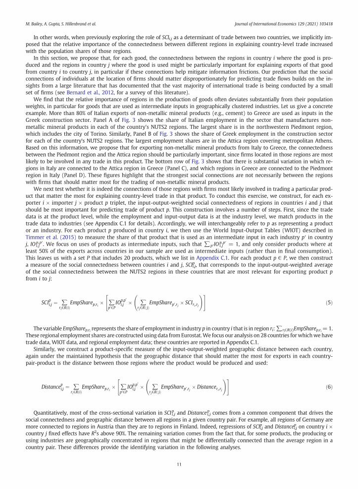
We find that the relative importance of regions in the production of goods often deviates substantially from their populationweights, in particular for goods that are used as intermediate inputs in geographically clustered industries. Let us give a concreteexample. More than 80% of Italian exports of non-metallic mineral products (e.g., cement) to Greece are used as inputs in theGreek construction sector. Panel A of Fig. 3 shows the share of Italian employment in the sector that manufactures non-metallic mineral products in each of the country's NUTS2 regions. The largest share is in the northwestern Piedmont region,which includes the city of Torino. Similarly, Panel B of Fig. 3 shows the share of Greek employment in the construction sectorfor each of the country's NUTS2 regions. The largest employment shares are in the Attica region covering metropolitan Athens.Based on this information, we propose that for exporting non-metallic mineral products from Italy to Greece, the connectednessbetween the Piedmont region and the Attica region should be particularly important, since firms located in those regions are mostlikely to be involved in any trade in this product. The bottom row of Fig. 3 shows that there is substantial variation in which re-gions in Italy are connected to the Attica region in Greece (Panel C), and which regions in Greece are connected to the Piedmontregion in Italy (Panel D). These figures highlight that the strongest social connections are not necessarily between the regionswith firms that should matter most for the trading of non-metallic mineral products.

We next test whether it is indeed the connections of those regions with firms most likely involved in trading a particular prod-uct that matter the most for explaining country-level trade in that product. To conduct this exercise, we construct, for each ex-porter i × importer j × product p triplet, the input-output-weighted social connectedness of regions in countries i and j thatshould be most important for predicting trade of product p. This construction involves a number of steps. First, since the tradedata is at the product level, while the employment and input-output data is at the industry level, we match products in thetrade data to industries (see Appendix C.1 for details). Accordingly, we will interchangeably refer to p as representing a productor an industry. For each product p produced in country i, we then use the World Input-Output Tables (WIOT) described inTimmer et al. (2015) to measure the share of that product that is used as an intermediate input in each industry p′ in countryj, IO i, j

p,p′. We focus on uses of products as intermediate inputs, such that ∑p′IO i, jp,p′ = 1, and only consider products where at

least 50% of the exports across countries in our sample are used as intermediate inputs (rather than in final consumption).This leaves us with a set P that includes 20 products, which we list in Appendix C.1. For each product p ∈ P, we then constructa measure of the social connectedness between countries i and j, SCIi,jp , that corresponds to the input-output-weighted averageof the social connectedness between the NUTS2 regions in these countries that are most relevant for exporting product pfrom i to j:

SCIpi,j ¼ ∑ri∈R ið Þ

EmpSharep,ri � ∑p0∈P

IOp,p0

i,j � ∑rj∈R jð Þ

EmpSharep0 ,rj � SCIri ,rj

!" #ð5Þ

The variable EmpSharep,ri represents the share of employment in industry p in country i that is in region ri:∑ri∈R(i)EmpSharep,ri=1.These regional employment shares are constructed using data fromEurostat.We focus our analysis on 28 countries forwhichwe havetrade data, WIOT data, and regional employment data; these countries are reported in Appendix C.1.

Similarly, we construct a product-specific measure of the input-output-weighted geographic distance between each country,again under the maintained hypothesis that the geographic distance that should matter the most for exports in each country-pair-product is the distance between those regions where the product would be produced and used:

Distancepi,j ¼ ∑ri∈R ið Þ

EmpSharep,ri � ∑p0∈P

IOp,p0

i,j � ∑rj∈R jð Þ

EmpSharep0 ,rj � Distanceri ,rj

!" #ð6Þ

Quantitatively, most of the cross-sectional variation in SCI i,jp and Distancei,j

p comes from a common component that drives thesocial connectedness and geographic distance between all regions in a given country pair. For example, all regions of Germany aremore connected to regions in Austria than they are to regions in Finland. Indeed, regressions of SCIi,jp and Distancei,j

p on country i ×country j fixed effects have R2s above 90%. The remaining variation comes from the fact that, for some products, the producing orusing industries are geographically concentrated in regions that might be differentially connected than the average region in acountry pair. These differences provide the identifying variation in the following analyses.

11

Fig. 3. Regional Employment Shares And Social Connectedness. Note: Panel A plots the regional shares of employment in the non-metallic minerals industry acrossNUTS2 regions in Italy. Panel B plots the regional shares of employment in the construction sector across NUTS2 regions in Greece. Panels C and D, respectively,show heat maps of social connectedness from the Attica Region in Greece to Italian NUTS2 regions, and from the Piedmont Region in Italy to Greek NUTS2 regions.


We then explore how trade in different products correlates with the product-specific measures of social connectedness, SCI i,jp ,and geographic distance, Distancei,jp , by estimating the following regression:

Xi,j,p ¼ exp β1 log SCIi,j� �

þ β2 log Distancei,j� �

þ β3 log SCIpi,j� �

þ β4 log Distancepi,j� �

þ δi,j,ph i

⋅εi,j,p ð7Þ

Here, Xi,j,p denotes the total value of exports of product p from country i to country j. We also include the logarithm ofpopulation-weighted measures of social connectedness and distance as controls; these are the same covariates that we used inSection 2. The vector δi,j,p represents various fixed effects. In all specifications we add country i × product p fixed effects aswell as country j × product p fixed effects, which controls for the average propensity of each country to export and importeach good.

Table 3 shows results from regression 7. In column 1, we control only for the population-weighted social connectedness anddistance. The estimated elasticity of trade to social connectedness is similar to that estimated in Section 2. This suggests that theset of countries and products for which we can construct input-output-weighted social connectedness has similar trade elasticitiesto the full sample of countries. In column 2, we instead control for the product-specific input-output-weighted social connected-ness between countries i and j. The magnitudes of the trade elasticities are similar to those in column 1. As discussed above, this isconsistent with the fact that much of the regional variation in social connectedness is explained by a component that is commonfor all region pairs in a country pair.

12

Table 3Input-output-weighted Social Connectedness and Trade in 2017.

Dependent variable: Product-Specific Bilateral Trade

(1) (2) (3) (4) (5) (6) (7)

log(SCI) 0.279*** −0.037(0.022) (0.123)

log(Distance) −0.975*** −0.365*(0.052) (0.203)

log(SCIp) 0.255*** 0.296** 0.303** 0.333** 0.268* 0.424***(0.022) (0.125) (0.148) (0.139) (0.154) (0.149)

log(Distancep) −0.944*** −0.588*** −1.020*** −0.305(0.052) (0.196) (0.196) (0.303)

Origin Country × Product FE Y Y Y Y Y Y YDestination Country × Product FE Y Y Y Y Y Y YUndir. Country Pair FE Y Ylog(Distancep) Group FE Y YUndir. Country Pair × Product FE Y YR2 0.953 0.955 0.955 0.970 0.971 0.990 0.991N 15,120 15,120 15,120 15,120 15,120 15,120 15,120N - Explained by FE 262 591 591 591 591 2,488 2,488

Note: Table shows the results from regression 7. The dependent variable is exports of product k from country i to country j in 2017. The variable SCIi,j is the pop-ulation-weighted average of NUTS2 region-level social connectedness. The variable SCIi,jp is an employment share-weighted measure as defined in eq. 5. The mea-sures Distancei,j and Distancei,jp are constructed in the same way as the corresponding social connectedness measures. All specifications include origin country ×product and destination country × product fixed effects. Columns 4 and 5 add country pair fixed effects that do not distinguish the direction of trade (undirected).Columns 6 and 7 include fixed effects that interact the undirected country pair fixed effects with product fixed effects. In columns 5 and 7, we replace the controlfor log(Distancei,jp ) with 100 dummy variables representing percentiles of the distance distribution. Standard errors are clustered by origin × destination countrypair. The data include 28 countries and 20 products leading to 15,120 (= 28 × 27 × 20) observations. Observations that are fully explained by the fixed effectsare dropped before the PPML estimation. Significance levels: *(p<0.10), **(p<0.05), ***(p<0.01).


In column 3, we control for both the population-weighted and input-output-weighted measures of social connectedness.While these two objects have a correlation of 95%, the regression loads strongly on the input-output-weighted measure of socialconnectedness—once this is controlled for, the population-weighted social connectedness has no additional predictive power. Thisfinding suggests that what matters for the trade in a specific product is the social connectedness across the regions that produceand use that specific good, instead of the social connectedness across the most heavily populated regions.

In columns 4 and 5, we include fixed effects for each country pair; relative to the specification in column 4, in column 5 wereplace the linear control for log(Distancei,jp ) with dummies for percentiles of the distribution of that variable. The newly intro-duced country pair fixed effects fully absorb the population-weighted social connectedness and geographic distance betweencountry pairs. Importantly, the inclusion of these fixed effects also controls for any other observable or unobservable factorsthat might have been correlated with both social connectedness and trade flows for a given country pair, and which wouldhave thus caused an omitted variables bias in the previous regressions. For example, including country pair fixed effects controlsfor whether countries share a common language, a common religion, or a common historical origin, all of which might be corre-lated both with trade flows and social connectedness. The estimated elasticity of trade flows to the product-specific input-output-weighted social connectedness is essentially unchanged in this specification.14

One specific concern alleviated by the specifications in columns 4 and 5 of Table 3 is that the correlation between country-levelsocial connectedness and trade documented in Section 2 might be the result of common preferences in consumption. Under thisalternative theory, higher social connectedness between the populations of two countries coincides with more similar consump-tion preferences of the populations, for example because social connectedness is partially driven by migration, and migrantshave similar preferences to people in their countries of origin. This similiarity of preferences might then be the source of tradein both final consumption goods and intermediate goods used in the production of the consumption goods (see Linder, 1961).However, if such an omitted variable explained the patterns in Section 2, the population-weighted social connectedness across re-gions would be the most powerful predictor of trade between countries, since it provides the most appropriate measure of thesimilarity of preferences between the populations. In contrast, we find that it is the social connectedness between the locationsof output and input industries for each product that determines the amount of trade. This finding suggests that similarities in pref-erences between more connected countries does not constitute a quantitatively important determinant of trade within Europe.

In columns 6 and 7 of Table 3, we include fixed effects that interact each product type with undirected country i × country jpair fixed effects: in other words, we are comparing exports of a specific good from country i to country j to the exports of thesame good from country j to country i. The remaining variation in product-specific social connectedness comes from the factthat the industries that produce the product in each country are not located in the same regions as the industries that usethese products as an input: SCI i,jp′≠ SCI j,ip′. The inclusion of these fixed effects does not have a systematic effect on the estimateof the elasticity of trade with respect to social conectedness, providing further evidence that common preferences across countries(which would likely affect the trade of a given good in both directions) are not a large driver of the findings in Section 2.

14 InAppendix C.3, we use a randomization inference approach to provide additional evidence that the social connections that determine trade in specific products arethose between the regions where the product is produced in the exporting country and the regions where it is used in the importing country.

13


4.2. Ruling out reverse causality

Another benefit of exploring the input-output-weighted social connectedness is that it allows us to further address concernsregarding reverse causality as an explanation for the observed relationship between trade and social connectedness, whereby theobserved social connections are formed as a result of social interactions due to trade. Our approach starts from the observationthat, under the reverse causality story, the social connectedness between input-output-weighted regions should be systematicallylarger in magnitude than the social connectedness between population-weighted regions, since reverse causality would increasethe connectedness between those regions that are actually engaged in trade relative to the connectedness of other regions notengaged in trade. To test whether this is indeed the case, we construct for each country i × country j × product p triplet the differencebetween the input-output-weighted social connectedness and the population-weighted social connectedness across countries i and j.To interpret the magnitude of the differences, we express them as a fraction of the cross-sectional standard deviation of SCI i,jp :

15 WeEuropearailway

SCI_Divergencepi,j ¼SCIpi,j−SCIi,j

SD SCIpi,j� � ð8Þ

Fig. 4 shows a histogram of SCI_Divergencei,jp across all 15,120 country i × country j × product p triplets. The distribution has amean of 0.008, and a median of −0.003. In other words, the regions that were shown to be most important for the trade in agiven product are equally likely to be more connected or less connected than the population-weighted average of regions acrossa country pair. This provides strong evidence against a quantitatively large reverse causality story in which the fact that two re-gions trade more with each other causes them to be meaningfully more socially connected.

4.3. Subnational social connectedness, rail freight flows, and the border effect in trade

In the final part of the paper, we study the relationship between regional social connectedness and subnational trade flows.This analysis allows us to examine the determinants of the border effect—the empirical regularity that, conditional on the distancebetween two regions, trade is much larger between regions that are part of the same country (see McCallum, 1995; Anderson andVan Wincoop, 2003).

A common challenge for exploring the border effect is the absence of systematic and large-scale trade data at the subnationallevel. However, within Europe, we observe data on rail freight tonnage shipped in 2015 between pairs of NUTS2 regions for a num-ber of countries (rail freight transport accounted for 12.2% of all intra-EU freight transport in 2015).15 We explore the relationshipbetween rail freight flows and social connectedness across European NUTS2 regions using the following regression:

RailFreightri ;r j ¼ exp β1 log SCIri ;r j

� �þ β2 log Distanceri ;r j

� �þ β31

SameCountryri ;r j

þ δri ;r jh i

� εri ;r j ð9Þ

The dependent variable, RailFreightri,rj, is the amount of goods (in tons) shipped by rail from region ri to region rj. The variableslog(SCIri,rj) and log(Distanceri,rj) are the logarithms of the social connectedness and distance between NUTS2 regions, respectively,and δri,rj represents various fixed effects. The dummy variable 1SameCountry

ri ;r j captures whether region ri and region rj are part of the

same country.Table 4 presents the results from regression 9. Column 1 does not yet control for the social connectedness between regions.

Conditional on geographic distance, trade is about nine times larger between regions in the same country than between regionsin different countries. This estimate is the same order of magnitude as that of Chen (2004), who finds that EU countries tradeabout six times more with themselves than with other countries, and that of Tan (2016), who finds that truck freight shipmentsin Europe are 5.75 times higher for shipments within the same country. These estimated border effects are large in light of thefact that most countries in the sample are part of the European Common Market, and therefore face no formal barriers totrade such as tariffs; indeed, we find similar border effects when we restrict our sample to exclusively focus on NUTS2 regionsfrom countries within the single market.

In column 2, we include our measure of the social connectedness between regions. The elasticity of trade flows with respect tosocial connectedness is similar to that estimated at the country level above. The estimate of trade declines at the border drop dra-matically, from a border effect of 818% to a border effect of about 207%, a decline of more than 65%. In columns 3 and 4, we con-duct the same analysis as in columns 1 and 2, but replace our controls for geographic distance with dummy variables forpercentiles of the distance distribution. This ensures that the estimated border effect does not, in part, pick up non-linearitiesin the relationship between geographic distance and trade. In these specifications, the magnitude of the border effect declineseven more after the inclusion of controls for social connectedness, from 628% to 63%, an estimate that is barely significant atthe 10% level. These findings suggest that much of the reason we see border effects in trade is that social connectedness ismuch stronger across regions within countries than it is across equidistant regions in different countries.

use data on region-to-region rail goods transportmade available by Eurostat in the series tran_rt_rago. The data are built from individual country reports to thn Union on national and international rail transport in 2015. For each pair of NUTS2 regions ri and rj, the data include the tons of goods that were loaded onvehicle in region ri and unloaded in region rj. We take a number of steps to standardize and clean the data, as described in Appendix C.2.

14

ea

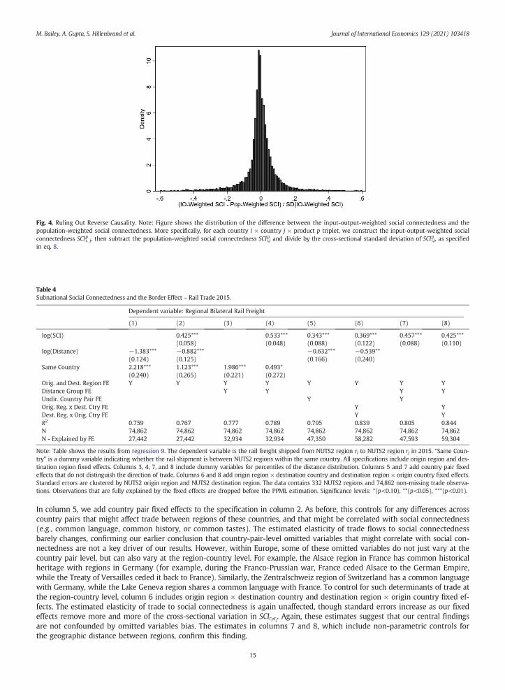
Fig. 4. Ruling Out Reverse Causality. Note: Figure shows the distribution of the difference between the input-output-weighted social connectedness and thepopulation-weighted social connectedness. More specifically, for each country i × country j × product p triplet, we construct the input-output-weighted socialconnectedness SCIi, j

p , then subtract the population-weighted social connectedness SCIi,jp and divide by the cross-sectional standard deviation of SCIi,jp , as specified

in eq. 8.

Table 4Subnational Social Connectedness and the Border Effect – Rail Trade 2015.

Dependent variable: Regional Bilateral Rail Freight

(1) (2) (3) (4) (5) (6) (7) (8)

log(SCI) 0.425*** 0.533*** 0.343*** 0.369*** 0.457*** 0.425***(0.058) (0.048) (0.088) (0.122) (0.088) (0.110)

log(Distance) −1.383*** −0.882*** −0.632*** −0.539**(0.124) (0.125) (0.166) (0.240)

Same Country 2.218*** 1.123*** 1.986*** 0.493*(0.240) (0.265) (0.221) (0.272)

Orig. and Dest. Region FE Y Y Y Y Y Y Y YDistance Group FE Y Y Y YUndir. Country Pair FE Y YOrig. Reg. x Dest. Ctry FE Y YDest. Reg. x Orig. Ctry FE Y YR2 0.759 0.767 0.777 0.789 0.795 0.839 0.805 0.844N 74,862 74,862 74,862 74,862 74,862 74,862 74,862 74,862N - Explained by FE 27,442 27,442 32,934 32,934 47,350 58,282 47,593 59,304

Note: Table shows the results from regression 9. The dependent variable is the rail freight shipped from NUTS2 region ri to NUTS2 region rj in 2015. “Same Coun-try” is a dummy variable indicating whether the rail shipment is between NUTS2 regions within the same country. All specifications include origin region and des-tination region fixed effects. Columns 3, 4, 7, and 8 include dummy variables for percentiles of the distance distribution. Columns 5 and 7 add country pair fixedeffects that do not distinguish the direction of trade. Columns 6 and 8 add origin region × destination country and destination region × origin country fixed effects.Standard errors are clustered by NUTS2 origin region and NUTS2 destination region. The data contains 332 NUTS2 regions and 74,862 non-missing trade observa-tions. Observations that are fully explained by the fixed effects are dropped before the PPML estimation. Significance levels: *(p<0.10), **(p<0.05), ***(p<0.01).


In column 5, we add country pair fixed effects to the specification in column 2. As before, this controls for any differences acrosscountry pairs that might affect trade between regions of these countries, and that might be correlated with social connectedness(e.g., common language, common history, or common tastes). The estimated elasticity of trade flows to social connectednessbarely changes, confirming our earlier conclusion that country-pair-level omitted variables that might correlate with social con-nectedness are not a key driver of our results. However, within Europe, some of these omitted variables do not just vary at thecountry pair level, but can also vary at the region-country level. For example, the Alsace region in France has common historicalheritage with regions in Germany (for example, during the Franco-Prussian war, France ceded Alsace to the German Empire,while the Treaty of Versailles ceded it back to France). Similarly, the Zentralschweiz region of Switzerland has a common languagewith Germany, while the Lake Geneva region shares a common language with France. To control for such determinants of trade atthe region-country level, column 6 includes origin region × destination country and destination region × origin country fixed ef-fects. The estimated elasticity of trade to social connectedness is again unaffected, though standard errors increase as our fixedeffects remove more and more of the cross-sectional variation in SCIri,rj. Again, these estimates suggest that our central findingsare not confounded by omitted variables bias. The estimates in columns 7 and 8, which include non-parametric controls forthe geographic distance between regions, confirm this finding.

15


5. Conclusion

In this paper, we use de-identified data from Facebook to construct a comprehensive measure of the social connectedness be-tween countries and between subnational regions. We use this measure to study the relationship between social connectednessand trade flows. Our findings on how social connections shape trade patterns provide new evidence for how social interactionscan determine financial and economic outcomes (see Hirshleifer, 2020; Kuchler and Stroebel, 2020).

We hope that our easily accessible measures of social connectedness will be used to broaden our understanding of the eco-nomic effects of social networks across a range of settings beyond international trade. For example, an exciting theoretical liter-ature suggests that social interactions shape financial market outcomes (Akcay and Hirshleifer, 2020; Hirshleifer, 2020) and thatthe diversity of social networks is an important determinant of economic development; conversely, tightly clustered social ties canlimit access to a broad range of social and economic opportunities (for example Granovetter, 1977, 2005; Chetty et al., 2020). Ourdata can help researchers test these and other predictions on the relationship between social structure and socio-economic out-comes. More generally, our research emphasizes the increasingly important role of data from online services—such as Facebook,LinkedIn, Twitter, eBay, Mint, Trulia, and Zillow—in overcoming important measurement challenges across the social sciences (see,for example, Baker, 2018; Giglio et al., 2015; Einav et al., 2015; Piazzesi et al., 2015; Bailey et al., 2020b).

6. Acknowledgments

We thank numerous seminar and conference participants, as well Treb Allen (Editor), Nick Bloom, Tarek Hassan, Peter Koudijs,Brent Neiman, Paola Sapienza, Alexi Savov, Tim Schmidt-Eisenlohr, Mike Waugh, Chenzi Xu, Moto Yogo, and two anonymous ref-erees for helpful comments. We also thank Dominic Russel and Steven Zheng for superb research assistance. This project was fa-cilitated through a research consulting agreement between some of the academic authors (Kuchler and Stroebel) and Facebook.Bailey is an employee at Facebook. The data on social connections used in this paper is available at https://data.humdata.org/dataset/social-connectedness-index.

Declaration of Competing Interest

None.

Appendix A. The determinants of international social connectedness

In Appendix A.1, we explore a number of further case studies of the social connectedness of individual countries. InAppendix A.2, we formally analyze the role of geography and other factors such as similarity of language, history, religion, andeconomic development in shaping international social connections.

A.1. Case studies of international social connectedness

Figs. A.1 to A.5 present heat maps of the social connections of several countries in addition to the heat map of Portugal's in-ternational connections in Panel A of Fig. 1. As before, darker colors correspond to closer connections.

A.1.1. India and MalaysiaFig. A.1 shows the social connectedness of two Asian countries, India (Panel A) and Malaysia (Panel B). Both countries are

strongly connected to the countries on the Arab peninsula, likely a result of migrant workers from India and Malaysia movingto work in these countries in recent years. Similarly, Malaysia is strongly connected to Nepal, likely due to a guest worker pro-gram allowing Nepalis to work in Malaysia. Social connections also appear to reflect earlier episodes of migrant and forcedlabor movements. For instance, India is strongly connected to Guyana in South America. In the 19th century, there was a lackof plantation workers following the abolition of slavery in this former European colony. Indians were selected to fill the gap asthey were used to working under tropical conditions and willing to accept cheap terms (Davis, 1951), and the resulting socialconnections to India appear to remain a century later. Finally, the Muslim-majority Malaysia is more strongly connected to thepredominantly Muslim countries on the Indian subcontinent (Pakistan, Bangladesh, and the Maldives) than it is connected toIndia itself, suggesting a role of religion in shaping today's social connections.

A.1.2. ArgentinaFig. A.2 shows the social connectedness of Argentina. Argentina is strongly connected to all Spanish-speaking countries in Latin

America. Connections to Portuguese-speaking Brazil are substantially weaker, even though the two countries are geographicallyclose and share a common border. Similarly, Argentina's strongest connection in Europe is to Spain. It is much less connectedto Italy, despite the fact that Italians were the largest group of post-colonial immigrants (more than from Spain) and 60% ofArgentinians have some Italian ancestry. These findings suggest an important role of shared language for today's connections.

A.1.3. Morocco and MauritaniaFig. A.3 shows the social connectedness of two neighboring countries in Northwest Africa, Morocco (Panel A) and Mauritania

(Panel B). Both Morocco and Mauritania are former French colonies and, as such, still have strong social ties to France. The populations

16



Fig. A.1. Social connectedness of India and Malaysia. Note: Figures show a heat map of the social connectedness of India (Panel A) and Malaysia (Panel B). For eachcountry in our data, the colors highlight connections to the focal country, given in red. The lightest color corresponds to the 20th percentile of the connectedness tothe focal country; darker colors correspond to closer connections. (For interpretation of the references to color in this figure legend, the reader is referred to theweb version of this article.)


17

Fig. A.2. Social Connectedness of Argentina. Note: Figure shows a heat map of the social connectedness of Argentina. For each country in the world, the colorshighlight connections to the focal country, given in red. The lightest color corresponds to the 20th percentile of the connectedness to the focal country; darkercolors correspond to closer connections. (For interpretation of the references to color in this figure legend, the reader is referred to the web version of this article.)


of both countries are predominantly Muslim, which helps to explain their strong ties to other Muslim countries in Northern Africa andthe Middle East. On the other hand, Mauritania has much stronger ties to Sub-Saharan Africa than Morocco does. This is likely relatedto the fact that Morocco's population is almost entirely Arab-Berber, while Mauritania has a substantial population of Haratin and WestAfrican ethnicity. These patterns suggest that ethnic ties are important in shaping friendships across countries.

A.1.4. Azerbaijan and TurkeyFig. A.4 shows the social connectedness of Azerbaijan (Panel A) and Turkey (Panel B), two countries in Northwest Asia that

share a short border. Both are strongly connected to each other, the nearby Caucasus countries of Armenia and Georgia, and Cen-tral European countries which have welcomed migrants from the two nations. However, Azerbaijan, a former Soviet Republic, ismuch more connected with countries in Europe and Central Asia that were also part of the Soviet Union, including Russia,Kazakhstan, Uzbekistan, Ukraine, Belarus, Lithuania, Latvia, and Estonia. Turkey, whose residents are predominately Muslim, ismore connected to other predominately Muslim countries including Afghanistan, Syria, Lebanon, Iraq, Saudi Arabia, Yemen, andLibya. These patterns emphasize that historical ties and religion play important roles in shaping today's social connections.

A.1.5. FijiPanel B of Fig. A.5 shows the social connectedness of Fiji. Fiji, a former British colony, is strongly connected to other countries

that were part of the British empire in Oceania (Australia, New Zealand, Papua New Guinea, and the Solomon Islands), as well asother English-speaking nations, including Canada, the United States, the United Kingdom, and Guyana. The country's connectionsto Guyana and Suriname are particularly strong compared to its connections with countries throughout the rest of South America.A potential explanation for this lies in the Indian worker program described previously. Between 1830 and 1930, over a millionindentured laborers from India were relocated to European colonies, including Dutch Suriname and British Fiji and Guyana.These patterns suggest that ties from migratory movements significantly impact international connectedness.

A.2. Regression analysis

The case studies above suggest that several factors such as geographic distance, colonial history, and past migration shapetoday's social connections between countries. We next estimate the following regression to analyze the contributions of these fac-tors to social connectedness more systematically:

log SCIi,j� �

¼ β þ γGi,j þ δi þ δj þ εi,j ðA:1Þ

18

Fig. A.3. Social connectedness of Morocco and Mauritania. Note: Figures show a heat map of the social connectedness of Morocco (Panel A) and Mauritania (PanelB). For each country in the world, the colors highlight connections to the focal country, given in red. The lightest color corresponds to the 20th percentile of theconnectedness to the focal country; darker colors correspond to closer connections. (For interpretation of the references to color in this figure legend, the reader isreferred to the web version of this article.)


19

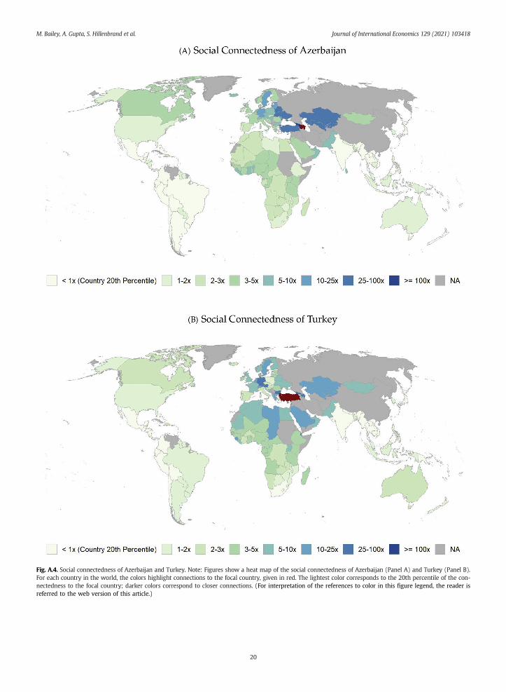
Fig. A.4. Social connectedness of Azerbaijan and Turkey. Note: Figures show a heat map of the social connectedness of Azerbaijan (Panel A) and Turkey (Panel B).For each country in the world, the colors highlight connections to the focal country, given in red. The lightest color corresponds to the 20th percentile of the con-nectedness to the focal country; darker colors correspond to closer connections. (For interpretation of the references to color in this figure legend, the reader isreferred to the web version of this article.)


20

Fig. A.5. Social Connectedness of Fiji. Note: Figure shows a heat map of the social connectedness of Fiji. For each country in the world, the colors highlight con-nections to the focal country, given in red. The lightest color corresponds to the 20th percentile of the connectedness to the focal country; darker colors correspondto closer connections. (For interpretation of the references to color in this figure legend, the reader is referred to the web version of this article.)


The dependent variable is the logarithm of the Social Connectedness Index between country i and country j. The vector Gi,j cap-tures variables that might explain international social connectedness. We also include fixed effects for each country, δi and δj, toabsorb any country-specific factors that may affect our measure of a country's connections to others, such as patterns of Facebookusage or internet penetration.

A.2.1. Geography and social connectednessWe first explore the role of geographic proximity in shaping international social connectedness. We measure the geographic

distance between two countries as the population-weighted distance given by CEPII; summary statistics are presented inTable A.1. The binscatter plots in Fig. A.6 show a broadly log-linear relationship between distance and social connectedness,both with and without country fixed effects. For large distances, the relationship becomes slightly convex, indicating that distancematters somewhat less once countries are already far apart.

Table A.2 explores the role of distance using regression A.1. Column 1 includes only fixed effects for country i and country j.The results suggest that about 30% of the pairwise connectedness of countries is explained by the fact that countries differ in theiraverage degree of global connectedness. In other words, most of the cross-sectional variation in social connectedness across coun-try pairs is the result of characteristics that vary at the country pair level, and not characteristics that vary at the country level.

Column 2 adds log(Distancei,j) as a control to the country fixed effects; this specification corresponds to the binscatter plots inPanel B of Fig. A.6. The estimates imply that a 10% increase in the geographic distance between countries is associated with a16.2% decline in social connectedness. In terms of magnitude, this elasticity is similar to the elasticity of connectedness to geo-graphic distance between U.S. counties in Bailey et al. (2018a). Moreover, geographic distance explains more than one half ofthe variation in social connectedness across countries after accounting for country fixed effects.

Column 3 explores the importance of potential non-linearities in the relationship between geographic distance and social con-nectedness. Specifically, instead of controlling for log(Distancei,j) linearly, we include dummy variables for percentiles of log(Distancei,j). The R2 of the regression is only slightly higher—67.5% instead of 66.6%– when we control for these percentiles.This finding confirms that the baseline log-linear specification is reasonable. Nevertheless, in columns 4 and 5 of Table A.2, wesplit the sample into country pairs that are more or less than 6,000 km apart. The estimated elasticity is −1.89 for countriesless than 6,000 km apart, and −0.90 for countries more than 6,000 km apart.

Column 6 of Table A.2 explores whether sharing a border increases social connectedness beyond geographic distance. For in-stance, a direct border may make it more likely that residents frequently spend time in the other country, either for work or lei-sure. It might also induce governments to cooperate and establish policies fostering cross-country interactions. Consistent withthese hypotheses, the estimates indicate that citizens of two countries that share a border are about twice as likely to be friendswith each other compared with citizens of two countries that are equally far apart but that do not share a border. However, theincremental R2 of including this additional control over distance alone is relatively small at 0.2%, since the common border

21

Table A.1Summary Statistics and Data Sources.

Mean P10 P25 P50 P75 P90 N Source

log(SCI) 7.72 5.83 6.44 7.37 8.66 10.13 28,730 Facebooklog(Distance) 8.78 7.69 8.43 8.95 9.32 9.60 28,730 CEPIIlog(1+Migrant Population) 2.44 0.00 0.00 0.00 4.81 8.02 28,392 United NationsCommon Colonizer 0.11 0.00 0.00 0.00 0.00 1.00 28,730 CEPIIColonial Relationship 0.01 0.00 0.00 0.00 0.00 0.00 28,730 CEPIIGenetic Distance 0.04 0.01 0.02 0.04 0.05 0.06 24,806 Spolaore et al. (2018)Common Official Language 0.16 0.00 0.00 0.00 0.00 1.00 28,730 CEPIIReligious Distance 0.75 0.54 0.66 0.80 0.86 0.96 25,760 Spolaore et al. (2016)Δ GDP per Capita (in ‘00,000$s) 0.19 0.01 0.03 0.10 0.28 0.51 28,730 CEPIICommon Border 0.02 0.00 0.00 0.00 0.00 0.00 28,730 CEPIISame Continent 0.22 0.00 0.00 0.00 0.00 1.00 28,730 UNStatsSame Subcontinent 0.12 0.00 0.00 0.00 0.00 1.00 28,730 UNStats

Note: Table presents summary statistics of variables used in Appendix A. Variables include the logarithm of SCI, the logarithm of distance, the logarithm of 1 plusthe average migrant population, a dummy indicating whether the pair of countries had a common colonizer post-1945, a dummy indicating whether the pair ofcountries was in a colonial relationship post-1945, genetic distance following Spolaore and Wacziarg (2018), a common official language dummy, religious distancefollowing Spolaore and Wacziarg (2016), differences in GDP per capita (in hundred thousands of dollars), a common border dummy, a same continent dummy,and a same subcontinent dummy.


indicator does not allow us to understand the substantial variation in connectedness between the vast majority of pairs of non-neighboring countries.

We also examine how continental borders shape friendships between countries. Following UNStats, we group countries intofive continents—Africa, the Americas, Asia, Europe, and Oceania—and into subcontinents such as Northern Africa and Sub-Saharan Africa. The regression results in column 7 of Table A.2 show that countries on the same subcontinent are about twiceas connected as two countries that are equally far apart but on different continents, all else equal. Being on the same continent(but not the same subcontinent) is associated with a 76% increase in social connectedness relative to two countries that areequally far apart but on different continents. Column 8 explores whether sharing a continent affects friendships differently on dif-ferent continents. Countries in Oceania and Africa are substantially more likely to be socially connected to other countries on thesame continent than predicted purely by geographic distance. On the other hand, countries in the Americas are not significantlymore likely to be connected to each other than to countries on a different continent that are equally far away.

A.2.2. Social connectedness and country similarityThe previous results highlight that various measures of geographic proximity can explain a little over half of the variation

in social connectedness across country pairs that is not explained by country fixed effects. We next explore the role of otherfactors in explaining international friendship linkages. Specifically, we analyze the role of past migration, colonial history,genetic similarity, common language, religion, and similarity in GDP. Table A.1 shows summary statistics on these variables,as well as the data sources; not all variables are available for all country pairs. Table A.3 presents the cross-correlation ofthese gravity variables with the SCI and with each other. Naturally, many of the variables are somewhat correlated withone another: for example, countries that share a colonial history are more likely to have a common official language.

Fig. A.6. Social Connectedness vs. Geographic Distance. Note: Figures show binscatter plots of social connectedness and geographic distance. Panel A regresses log(SCI) on log(Distance) without any fixed effects, while Panel B controls for country fixed effects.

22

Table A.2The Geographic Determinants of Social Connectedness.

Dependent variable: log(SCI)

(1) (2) (3) (4) (5) (6) (7) (8)

log(Distance) −1.615∗∗∗ 100 −1.887∗∗∗ −0.899∗∗∗ −1.562∗∗∗ −1.092∗∗∗ −1.201∗∗∗

(0.038) Quantiles (0.060) (0.076) (0.039) (0.059) (0.052)Common border 0.755∗∗∗ 0.860∗∗∗ 0.858∗∗∗

(0.112) (0.115) (0.107)Same continent 0.760∗∗∗

(0.087)Same subcontinent 0.406∗∗∗

(0.116)Both in Africa 1.522∗∗∗

(0.159)Both in Americas 0.114

(0.114)Both in Asia 0.395∗∗∗

(0.111)Both in Europe 0.779∗∗∗

(0.168)Both in Oceania 2.668∗∗∗

(0.327)Orig. and Dest. Country FE Y Y Y Y Y Y Y YSample All All All < 6000 km > 6000 km All All AllR2 0.303 0.666 0.675 0.662 0.552 0.668 0.693 0.706N 28,730 28,730 28,730 10,594 18,136 28,730 28,730 28,730

Note: Table shows results of regression A.1. The dependent variable is the logarithm of social connectedness for a country pair. Explanatory variables includethe logarithm of distance, a dummy indicating a common border, a same continent dummy, a same subcontinent dummy, and dummies indicating whetherthe pair of countries belongs to Africa, the Americas, Asia, Europe or the Oceania region. In column 3, the logarithm of distance is replaced by indicators basedon 100 quantiles of distance. All specifications include fixed effects for the origin and destination country. Standard errors are clustered by origin and destinationcountry. We have data on social connectedness for 170 countries, which leads to 28,730 (= 170 × 169) observations. Significance levels: ∗ (p<0.10), ∗∗ (p<0.05), ∗∗∗ (p<0.01).


Table A.4 contains the results from Regression A.1 when controlling for these variables. We first explore the relationshipsbetween the gravity variables and social connectedness separately for each variable, before analyzing them jointly in a mul-tivariate analysis.

A.2.2.1. Migration. It is likely that migrants retain many friends and family ties to their countries of origin. As a result, we wouldexpect that past migration patterns explain some of the observed cross-sectional variation in social connectedness. To measuremigration between country pairs, we use bilateral migration data from the Population Division of the Department of Economicand Social Affairs of the United Nations.16 The estimates in column 1 of Table A.4 show a strong relationship between past migra-tion and current social relationships. Doubling the average migrant population increases social connectedness between countriesby over 20%. Including migration in addition to distance and country fixed effects increases the R2 of the regression by 6.1 per-centage points.

Table A.3Correlation Table: Social Connectedness and Determinants.

(1) (2) (3) (4) (5) (6) (7) (8) (9) (10) (11) (12)

(1) log(SCI) 1.00(2) log(Distance) −0.60 1.00(3) log(1+Migrant Population) 0.38 −0.42 1.00(4) Common Colonizer 0.28 −0.03 −0.06 1.00(5) Colonial Relationship 0.10 −0.01 0.16 −0.03 1.00(6) Genetic Distance −0.42 0.57 −0.44 0.01 0.00 1.00(7) Common Official Language 0.45 −0.10 0.11 0.39 0.14 −0.01 1.00(8) Religious Distance −0.27 0.19 −0.17 0.03 0.00 0.08 −0.22 1.00(9) Δ GDP per Capita (in ‘00,000$s) 0.03 0.01 0.31 −0.11 0.06 −0.11 −0.02 −0.03 1.00(10) Common Border 0.27 −0.36 0.27 0.06 −0.00 −0.16 0.12 −0.12 −0.07 1.00(11) Same Continent 0.55 −0.65 0.25 0.10 −0.03 −0.39 0.18 −0.17 −0.15 0.23 1.00(12) Same Subcontinent 0.53 −0.52 0.12 0.12 −0.02 −0.25 0.27 −0.18 −0.22 0.28 0.71 1.00

Note: Table presents correlations between variables used in Appendix A. Variables include the logarithm of SCI, the logarithm of distance, the logarithm of 1 plusthe average migrant population, a dummy indicating whether the two countries had a common colonizer post 1945, a dummy indicating whether the pair of coun-tries was in a colonial relationship post 1945, genetic distance, a common official language dummy, religious distance, differences in GDP per capita (in hundredthousands of dollars), a common border dummy, a same continent dummy and a same subcontinent dummy.

23


A.2.2.2. Common colonial history. The case studies in Appendix A.1 suggest that countries with a common colonial history maintaincloser present-day social ties. To systematically explore this relationship, we use two measures of colonial history. Our first mea-sures is an indicator for having a common colonizer after 1945. The second measure is an indicator for having been in a colonialrelationship post 1945. The estimates in column 2 indicate that colonial history correlates strongly with social connectedness.Countries with a common colonizer have almost twice as many friendship links on Facebook as other countries that are similarlyfar apart. Having been in a colonial relationship increases the connectedness between countries by a factor close to three. Addingcontrols for colonial ties to distance and country fixed effects explains an additional 3.2% of the cross-sectional variation in socialconnectedness.

A.2.2.3. Genetic distance. Homophily suggests that there are likely to be more connections among countries whose populations aremore similar to each other, including along genetic lines. We measure genetic distance following Spolaore and Wacziarg (2018).17

Table A.3 shows that genetic distance has a raw correlation of −42% with social connectedness; this is reflected in the strong neg-ative relationship in the regression analysis. Going from the 10th percentile of genetic distance to the 90th percentile is associatedwith a decrease in social connectedness of 162%. Including genetic distance leads to an incremental increase in explanatory power,as measured by the R2, of just under 5%.

A.2.2.4. Common language. Language is a natural determinant of social relationships. After all, it is hard to form a personal relation-ship without speaking the same language. To formally explore the relationship between language and social connectedness, weuse an indicator variable for whether two countries share a common official language. The common language indicator is stronglycorrelated with social connections as evidenced by a raw correlation of 45% presented in Table A.3. Column 4 of Table A.4 con-firms the strong relationship. Having a common language more than doubles the social connectedness between two countries,and increases the R2 by 4.4 percentage points.

A.2.2.5. Similar religion. People of the same or similar religion may find it easier to connect to others who share their belief system.In addition, people of the same religion may be more likely to meet each other across countries, for instance when traveling forpilgrimage. To explore the effect of religion on social connectedness, we measure religious distance between countries followingSpolaore and Wacziarg (2016).18 The estimates in column 5 of Table A.4 suggest that social connections decrease by 65% whenmoving from the 10th percentile to the 90th percentile of religious distance. The incremental R2 of religion is less than 1%,which is less than the variation explained by the other variables explored so far.

A.2.2.6. Similarity in GDP. Bailey et al. (2018a) show that, at the individual level, people are more likely to be friends with others ofsimilar incomes. We next explore whether this is also true for international social connectedness. For each country pair, we com-pute the absolute difference in GDP per capita. Column 6 of Table A.4 shows that differences in GDP correlate with social connect-edness. A ten thousand dollar higher absolute difference in GDP per capita across two countries corresponds to a 13.1% decline insocial connectedness. However, differences in GDP only explain a small fraction of the cross-sectional variation in social connec-tions, with an incremental R2 of only 0.7%.

A.2.2.7. Multivariate regression. The first six columns of Table A.4 have shown the relationship between each regressor and socialconnectedness separately (in addition to controls for distance and country fixed effects). However, many of these variables arecorrelated with each other, as shown in Table A.3, and they often capture related aspects of across-country similarity. Column7 explores how much of the variation in social connectedness can be jointly explained by these variables. As expected, the esti-mated coefficients for most variables decrease somewhat, though almost all variables retain their economic and statistical signif-icance. The estimated effect of distance drops to about one third of the coefficient in the univariate regressions, suggesting thatdistance captures some aspects of the other cultural and social similarity in explaining social connectedness. Taken together,the incremental R2 of all additional regressors (beyond distance and fixed effects) is 14.1%.

As shown in Table A.3, a number of the control variables in Table A.4 are highly correlated. For example, the correlation be-tween genetic distance and our measure of migration is −0.44. Therefore, another interesting metric is how much explanatorypower each variable contributes when controlling for all other variables. For each variable, we run two regressions with the spec-ification in column 7 of Table A.4: one where we exclude the variable of interest and one where we include it. We then comparethe R2 of the two regressions, giving us an estimate of the incremental explanatory power of the variable beyond all other explan-atory variables. The results of this exercise are reported in Table A.5. We find that migration has the largest incremental R2 with3.24% followed by genetic distance with 2.16%. Geographic distance (1.85%) and the common official language dummy (1.00%)also add sizable explanatory power. Colonial heritage, religious distance, a common border, and being on the same subcontinenthave very little explanatory power once we control for other factors.

17 This measure of genetic distance is based on variation in the human DNA for ethnic groups from Pemberton et al., 2013 population and converted to a country-to-country measure using the shares of each ethnic group in each country's populations from Alesina 2003 fractionalization. It is therefore the expected genetic distancebetween two individuals randomly selected from the two countries.18 Thismeasure of religious distance between any two countries is based on two components: the distance between different religions and the share of the populationin a country that follow a religion. The proximity of two religions is based on how many nodes the two religions share in a tree describing the relationship betweendifferent religions. For instance, Roman Catholics aremore closely related to Orthodox Christians than toMuslims. The religious distance between two countries is thenobtained by summing across the distances of all religions while weighting each religion by the fraction of people in the two countries that follow the religion.

24

Table A.4The Determinants of Social Connectedness.

Dependent variable: log(SCI)

(1) (2) (3) (4) (5) (6) (7)

log(Distance) −1.172∗∗∗ −1.566∗∗∗ −1.235∗∗∗ −1.482∗∗∗ −1.539∗∗∗ −1.583∗∗∗ −0.612∗∗∗

(0.0418) (0.0341) (0.0368) (0.0410) (0.0418) (0.0366) (0.0492)log(1+Migrant Population) 0.218∗∗∗ 0.172∗∗∗

(0.0117) (0.0110)Common Colonizer 1.093∗∗∗ 0.431∗∗∗

(0.0862) (0.0614)In Colonial Relationship 1.959∗∗∗ 1.057∗∗∗

(0.226) (0.149)Genetic Distance −32.57∗∗∗ −22.87∗∗∗

(1.864) (1.662)Common Official Language 1.210∗∗∗ 0.643∗∗∗

(0.0770) (0.0614)Religious Distance −1.549∗∗∗ −0.542∗∗∗

(0.174) (0.124)Δ GDP per Capita (in ‘00,000$s) −1.305∗∗∗ −0.941∗∗∗

(0.284) (0.211)Common Border 0.0301

(0.101)Same Sontinent 0.594∗∗∗

(0.0667)Same Subcontinent −0.104

(0.0871)Orig. and Dest. Country FE Y Y Y Y Y Y YCoeff. on distance w/o regressors −1.614 −1.615 −1.616 −1.615 −1.610 −1.615 −1.608R2 0.722 0.694 0.714 0.705 0.671 0.669 0.807Incremental R2 of regressors 0.061 0.032 0.049 0.044 0.009 0.007 0.141N 28,392 28,730 24,806 28,730 25,760 28,730 23,562

Note: Table shows results of regression 1. The dependent variable is the logarithm of the social connectedness for a country pair. Independent variables include thelogarithm of distance, the logarithm of 1 plus the average migrant population, a dummy indicating whether the pair of countries had a common colonizer post-1945, a dummy indicating whether the pair of countries was in a colonial relationship post-1945, genetic distance, a common official language dummy, religiousdistance, differences in GDP per capita (in hundred thousands of dollars), a common border dummy, a same continent dummy and a same subcontinent dummy.All specifications include fixed effects for the origin and destination country. Standard errors are clustered by origin and destination country. We have data onsocial connectedness for 170 countries, which leads to 28,730(= 170 × 169) observations. Not all variables are available for all country pairs. Significance levels:∗ (p<0.10), ∗∗ (p<0.05), ∗∗∗ (p<0.01).


Appendix B. Trade and social connectedness

In this appendix, we present material complementary to our analysis of country-level trade in Section 2. Appendix B.1 explainsthe construction of the data, Appendix B.2 shows robustness to using OLS estimations instead of PPML, Appendix B.3 estimatestime-varying elasticities of trade to social connections, and Appendix B.4 runs a horse race between different gravity variablesin explaining international trade. Appendix B.5 studies the effects of social clusters on trade.

Table A.5Incremental Explanatory Power of Regressors for SCI.

Incremental R2 Dependent variable: log(SCI)

log(Distance) 1.85log(1+Migrant Population) 3.24Common Colonizer 0.33Colonial Relationship 0.20Genetic Distance 2.16Common Official Language 1.00Religious Distance 0.10Δ GDP per Capita (in ‘00,000$s) 0.33Common Border 0.00Same Continent 0.69Same Subcontinent 0.01

Note: Table reports the incremental R2 of each regressor when included/excluded in a regression of the logarithm of SCI on the full panel of regressors. This is alikethe specification in column 7 of Table A.4. To get the incremental R2, we compute the difference between the R2 of a regression when we exclude the variable fromthe set of explanatory variables and the R2 when we include the variable in the set of explanatory variables. For each variable considered, we run both regressionson the same set of observations.

25


B.1. Construction of trade and SCI data

For the analyses in Section 2, we merge data on international social connectedness with product-level trade data from CEPII. Ofthe 170 countries for which we have data on international social connectedness and gravity variables, five countries are not in-cluded in the trade data. These countries are Botswana, Lesotho, Luxembourg, Namibia, and Swaziland. In the original data, prod-ucts are classified according to the 6-digit HS96 classification into 4,914 product categories. In order to construct total bilateraltrade, used in Section 2, we aggregate trade across all products for each exporter-importer pair. We replace missing trade valueswith zero trade values. The final data that contains information on social connectedness, gravity variables, and aggregate bilateraltrade include 165 countries and 27,060(= 165 × 164) observations. In Section 3, we also use data on product-level trade insteadof total trade. For computational reasons, we aggregate trade flows up to the first two digits of the HS96 product code for eachexporter-importer pair. The first two digits of the product code are referred to as the “HS chapter”. For example, chapter 09 in-cludes “Coffee, Tea, Maté and Spices”. This procedure results in 96 product categories. We replace missing trade values withzeros. The panel on product-level trade and social connectedness contains 2,597,760(=165 × 164 × 96) observations.

B.2. Gravity regressions (OLS) - intensive margin of trade

Table 2 in Section 2 showed results from regressing aggregate bilateral trade on social connectedness and other gravity vari-ables. The regression was estimated using Poisson Pseudo Maximum Likelihood (PPML) to account for zero bilateral trade be-tween countries. Here, we show that the results are robust to estimating the relationships using OLS. We focus on theintensive margin of trade in order to avoid problems with zero-trade observations. We estimate the following regression:

log Xi,j

� �¼ β þ γGi,j þ δi þ δj þ εi,j ðB:1Þ

The dependent variable log(Xi,j) denotes the logarithm of the total value of exports from country i to country j. The results arereported in Table B.1. As before, social connectedness explains a substantial part of the variation in bilateral trade at the intensivemargin. Column 2 shows that social connectedness explains 29.5% of the within variation of trade after controlling for exporterand importer fixed effects, nearly as high as the within-R2 of 30.4% for distance (see column 3). Similarly to Table 1, column 4shows that gravity variables together explain a much smaller share of variation—here, less than half as much—than social connect-edness. Column 7 shows that, after controlling for distance and other gravity variables, the coefficient on social connectedness issimilar to that obtained using PPML (0.37 vs. 0.28). Overall, these results show that our baseline results are not an artefact of thespecific estimation method.

B.3. Time-variation in trade elasticities

In this section, we examine how the elasticity of trade with respect to social connectedness and distance varies over time. Forthis purpose, we use The Direction of Trade Statistics from the IMF that reports aggregate bilateral trade data from 1948 to 2018.Because the earlier years contain a lot of missing trade entries and we want to keep the set of countries constant across time, wefocus on the time period from 1981 to 2018. For each year, we regress aggregate bilateral trade on our distance measure and oursocial connectedness measure from August 2020. This allows us to estimate year-specific regression coefficients that are shown inFig. B.1. These findings highlight that the elasticity of trade to both distance and social connectedness has been highly constantover the past fourty years; the results also document that the underlying trade-facilitating relationships that we proxy for withthe Social Connectedness Index are very stable over time.

B.4. Gravity regressions – a horse race of predictors

In Table 2 of the main paper, we regressed aggregate bilateral trade flows on the logarithm of social connectedness and othergravity variables. However, it might be instructive to look at how trade interacts with each of these variables individually, explor-ing the relative economic and statistical significance of each variable separately.

In this section, we conduct this analysis using both PPML regressions as well as OLS regressions that study the intensive mar-gin of trade. We report the results of this “horse race of predictors” in Table B.2. Columns 1 to 6 are estimated using PPML, whilecolumns 7 to 12 are estimated using OLS. Consistent with our other results, we find that distance and social connectedness are themost successful in explaining variation in bilateral trade. In the PPML regression, distance and social connectedness are the onlytwo variables that individually explain more than 90% of bilateral trade after controlling for exporter and importer country fixedeffects. A similar results emerges from the OLS regression: including distance and social connectedness raises the R2 significantlycompared to all other gravity variables.

B.5. Groups of socially connected countries

One advantage of our measure of social connectedness is that it covers the vast majority of countries, allowing us to under-stand the structure of global social connectedness beyond just bilateral connections. In particular, we describe above that

26

Table B.1Gravity Regressions (OLS) - Intensive Margin of Trade - 2017.

Dependent variable: log(Aggregate Bilateral Trade)

(1) (2) (3) (4) (5) (6) (7) (8)

log(SCI) 0.773∗∗∗ 0.428∗∗∗ 0.368∗∗∗ 0.374∗∗∗

(0.0272) (0.0318) (0.0326) (0.0332)log(Distance) −1.711∗∗∗ −1.026∗∗∗ −1.547∗∗∗ −1.026∗∗∗

(0.0650) (0.0756) (0.0657) (0.0770)Common Border 3.671∗∗∗ 0.844∗∗∗ 0.692∗∗∗ 0.621∗∗∗

(0.237) (0.202) (0.188) (0.204)Common Official Language 1.258∗∗∗ 0.555∗∗∗ 0.194∗∗ 0.209∗∗

(0.153) (0.0903) (0.0818) (0.0829)Common Colonizer 0.902∗∗∗ 0.687∗∗∗ 0.362∗∗∗ 0.352∗∗∗

(0.190) (0.143) (0.119) (0.117)Colonial Relationship 0.591∗∗ 1.158∗∗∗ 0.645∗∗∗ 0.645∗∗∗

(0.269) (0.184) (0.146) (0.146)Orig. and Dest. Country FE Y Y Y Y Y Y Y YDistance Control Groups YN 18,393 18,393 18,393 18,393 18,393 18,393 18,393 18,393Adjusted R2 0.681 0.775 0.778 0.722 0.791 0.784 0.792 0.792

Note: Table shows results from regression B.1. We estimate the regression on non-zero trade observations (intensive margin) using OLS. The dependent variable istotal exports from country i to country j. Controls include the logarithm of SCI, the logarithm of distance, a common border dummy, a common official languagedummy, a dummy indicating whether the two countries had a common colonizer post-1945, a dummy indicating whether the pair of countries was in a colonialrelationship post-1945 and percentiles of SCI. All specifications include exporter and importer country fixed effects. Standard errors are clustered by exporter andimporter country. We have data on trade and social connectedness for 165 countries, which leads to 18,393 non-zero trade observations. Significance levels:*(p<0.10), **(p<0.05), ***(p<0.01).

Fig. B.1. Time-variation in Elasticity of Trade to Social Connectedness. Note: Figures show year-specific regression coefficients from regressing trade on log(SCI) andlog(Distance) as specified in Eq. (2). Panel A shows the regression coefficients obtained in univariate regressions, and Panel B shows the regression coefficientsobtained in multivariate regressions. The dark grey solid line shows the coefficient on social connectedness, while the light grey dashed line shows the coefficienton distance. Both regression specifications include exporter and importer country fixed effects.


countries that share certain characteristics are more socially connected to each other. Such shared characteristics often lead us tothink about groups of countries, such as “Spanish-speaking South America” or “Arab North Africa,” where countries in the groupare all similar to one another on some salient dimension. We next formalize the idea of groups of countries with strong connec-tions among each other. We then use this grouping to show that trade patterns are influenced not only by direct social connec-tions, but also by the social clusters that different countries are part of.

There are a number of possible algorithms to construct clusters of countries that feature a high average within-cluster pairwisesocial connectedness. Here, we use hierarchical agglomerative linkage clustering to group countries into 30 clusters.19 Fig. B.2

19 The agglomerative clustering algorithm starts by considering each of theN countries as a separate group of size one. In the first step, the two “closest” countries aremerged into one larger group, producingN− 1 total groups. In each subsequent step, the closest two groups are againmerged. This process continues until all the coun-tries are merged into a given number of clusters. We define the “distance” between two countries as the inverse of SCIi, j: the lower the probability of a given Facebookuser in country i knowing a given Facebook user in country j, the “further apart” socially the two countries are. We calculate the closeness between clusters with morethan one country as the average distance between the countries in the cluster.

27

Table B.2Gravity Regressions - Aggregate Trade in 2017 - Horse Race..

PPML OLS

Dependent variable: Aggregate Bilateral Trade Dependent variable: log(Aggregate Bilateral Trade)

(1) (2) (3) (4) (5) (6) (7) (8) (9) (10) (11) (12)

log(Distance) −0.992∗∗∗ −1.711∗∗∗

(0.0595) (0.0650)log(SCI) 0.646∗∗∗ 0.773∗∗∗

(0.0390) (0.0272)Common Border 1.905∗∗∗ 4.317∗∗∗

(0.208) (0.244)Common Official Language 0.908∗∗∗ 1.800∗∗∗

(0.145) (0.167)Common Colonizer 1.509∗∗∗ 1.642∗∗∗

(0.168) (0.209)Colonial Relationship 0.353 1.287∗∗∗

(0.303) (0.349)Orig. and Dest. Country FE Y Y Y Y Y Y Y Y Y Y Y YAdjusted R2 0.935 0.921 0.891 0.848 0.843 0.837 0.778 0.775 0.705 0.701 0.691 0.682N 27,060 27,060 27,060 27,060 27,060 27,060 18,393 18,393 18,393 18,393 18,393 18,393

Note: Table shows results from regression 2 (PPML) and regression B.1 (OLS). We estimate the regression using PPML in columns 1–6 and using OLS in columns7–12. The dependent variable is total exports from country i to country j for the PPML regressions, and the logarithm thereof for the OLS regressions. Controlsinclude the logarithm of SCI, the logarithm of distance, a common border dummy, a common official language dummy, a dummy indicating whether the two coun-tries had a common colonizer post-1945, and a dummy indicating whether the pair of countries was in a colonial relationship post-1945. All specifications includeexporter and importer country fixed effects. Standard errors are clustered by exporter and importer country. We have data on social connectedness for 165 coun-tries, which leads to 27,060(= 165 × 164) observations. The OLS regressions use only non-zero trade observations (intensive margin of trade). Significance levels:*(p<0.10), **(p<0.05), ***(p<0.01).


shows the 30 different clusters and Table B.3 lists the countries in each cluster. The average number of countries per cluster is 6.There are four clusters that only contain a single country — Brazil, Mexico, Burma, and Turkey. By far the largest cluster with 36countries contains all of Southern and Western Africa. All other clusters have substantially fewer countries, with the second andthird largest clusters containing 16 and 10 countries, respectively.

Different characteristics shape the different clusters. For instance, countries in Central America form one cluster, consistentwith the importance of geography. Spain, however, forms a cluster with Argentina, Uruguay, and Paraguay, highlighting thatnot all clusters are geographically contiguous and pointing at shared language as another important factor. The cluster comprisedof Mongolia and South Korea reflects both a long common history and common ethnic ancestry, as well as recent migration ofMongolians to South Korea. While standard characteristics can explain some of the variation in clustering, it is important to

Fig. B.2. Groups of socially connected countries: 30 clusters. Note: Figure shows countries grouped together when we use hierarchical agglomerative linkageclustering to create 30 distinct groups of socially connected countries.

28

Table 1230 Clusters of Socially Connected Countries.

Cluster Countries

1 Angola, Benin, Botswana, Burkina Faso, Burundi, Cameroon, Central African Republic, Chad, Congo, Cote d'Ivoire, Democratic Republic of the Congo,Equatorial Guinea, Gabon, Gambia, Ghana, Guinea, Kenya, Lesotho, Liberia, Malawi, Mali, Mauritania, Mozambique, Namibia, Niger, Nigeria, Rwanda,Senegal, Sierra Leone, South Africa, Swaziland, Togo, Uganda, United Republic of Tanzania, Zambia, Zimbabwe

2 Antigua and Barbuda, Bahamas, Barbados, Belize, Canada, Cayman Islands, Dominican Republic, Grenada, Guyana, Haiti, Jamaica, Saint Lucia, SaintVincent and the Grenadines, Suriname, Trinidad and Tobago, United States

3 Denmark, Estonia, Finland, Iceland, Ireland, Latvia, Lithuania, Norway, Sweden, United Kingdom4 Albania, Austria, Bosnia and Herzegovina, Croatia, Germany, Malta, Slovenia, Switzerland, Republic of North Macedonia5 Bahrain, Bangladesh, Kuwait, Maldives, Oman, Pakistan, Saudi Arabia, Sri Lanka, United Arab Emirates6 Australia, Fiji, Kiribati, New Zealand, Papua New Guinea, Samoa, Solomon Islands, Tonga, Vanuatu7 Belgium, Bulgaria, Cyprus, Greece, Italy, Netherlands, Republic of Moldova, Romania8 Brunei Darussalam, Hong Kong, Macau, Malaysia, Philippines, Singapore, Taiwan9 Costa Rica, El Salvador, Guatemala, Honduras, Nicaragua, Panama10 Bolivia, Chile, Colombia, Ecuador, Peru11 Cape Verde, Guinea-Bissau, Luxembourg, Portugal, Sao Tome and Principe12 Egypt, Jordan, Lebanon, Libyan Arab Jamahiriya, Palestine13 Argentina, Paraguay, Spain, Uruguay14 Bhutan, India, Nepal, Qatar15 Comoros, Madagascar, Mauritius, Seychelles16 Armenia, Azerbaijan, Georgia17 Belarus, Poland, Ukraine18 Czech Republic, Hungary, Slovakia19 Algeria, Morocco, Tunisia20 France, French Polynesia, New Caledonia21 Kazakhstan, Kyrgyzstan, Uzbekistan22 Cambodia, Lao People's Democratic Republic, Thailand23 Djibouti, Ethiopia24 Indonesia, Timor-Leste25 Japan, Viet Nam26 Republic of Korea, Mongolia27 Brazil28 Mexico29 Burma30 Turkey

Note: The table reports 30 groups generated by hierarchical agglomerative linkage clustering.


note that these clusters are constructed from our social connectedness measure that has substantial variation beyond standardgravity characteristics.

B.5.1. Groups of socially connected countries and tradeWe next explore the effect on trade of two countries sharing connections to a similar set of other countries, over and above

the direct effect of the bilateral connections between those two countries. There are several mechanisms through which beingin the same social cluster of countries could increase trade. Conceptually, being in the same social cluster can increase trade byalleviating search frictions. If country A and B are both connected to country C, traders in country A can use existing links to coun-try C in order to establish connections with potential trading partners in country B. We build two measures of whether countriesshare social connections with a similar set of other countries. Our first measure is simply a dummy variable for whether countriesare in the same one of the 30 clusters, though our results are robust to variations in the cluster size. Our second measure captureswhether countries are placed into the same cluster at an early, middle, or late stage of the agglomerative clustering process.20 Theadvantage of this measure is that it does not require us to take a stand on the number of clusters we put countries into.

We present the results from this analysis in Table B.4. For comparison, in column 1 we present our baseline specification foraggregate trade, corresponding to column 7 of Table 1. In column 2, we control for whether countries are in the same clusterwhen splitting the world into 30 groups. Conditional on the bilateral social connectedness and other gravity variables, being inthe same cluster increases trade substantially. As an example, Spain is approximately equally well-connected to the UnitedKingdom and to Argentina, but it only shares a cluster with Argentina. Our estimates suggest that, all else equal, Spain wouldthus trade 33% more with Argentina than with the United Kingdom.

In column 3, we interact the number of countries (in logs) in the cluster with the same-cluster dummy variable. We see thatthe effect on trade of being in the same cluster increases when the cluster includes a larger number of other countries. In column4, we add the dummy variables for when countries join the same cluster. We find that, controlling for the direct effect of bilateralsocial connectedness as well as the other gravity variables, countries which join the same cluster early rather than late have 21%

20 Agglomerative clustering is a sequential procedurewhere at each stage countries aremerged into clusters. Merging tends to occur earlier in the process if countriesare closer socially. Due to the nature of the hierarchical clustering algorithm, most countries do not join the same cluster until the last stage. We use cutoffs of 95% and90% to put country pairs into 3 groups for when they join the same cluster. These cutoffs correspond to the 18th and 41st clustering steps.

29

Table B.4Gravity Regressions - The Role of Social Clusters.

Dependent variable: Aggregate Exports

(1) (2) (3) (4) (5) (6) (7)

log(SCI) 0.280*** 0.262*** 0.280*** 0.267***(0.026) (0.025) (0.023) (0.025)

Same Cluster (30 Gr.) 0.286*** −0.544* 0.324*** 0.132(0.079) (0.298) (0.071) (0.239)

Join Same Cluster - Middle 0.144 0.160**(0.100) (0.069)

Join Same Cluster - Early 0.214* 0.433***(0.116) (0.114)

Same Cluster (30 Gr.) × log(Cluster Size) 0.389*** 0.091(0.146) (0.106)

Orig. and Dest. Country FE Y Y Y Y Y Y YOther Gravity Controls Y Y Y Y Y Y YSCI Group FE Y Y YDistance Group FE Y Y YR2 0.943 0.944 0.944 0.943 0.951 0.951 0.951N 27,060 27,060 27,060 27,060 27,060 27,060 27,060

Note: Table shows results from regression 2. The dependent variable is total exports from country i to country j. “Same Cluster (30 Gr.)” is a dummy variable in-dicating that the two countries are in the same cluster when we create 30 clusters using the hierarchical clustering algorithm described in Appendix B.5. “JoinSame Cluster” indicates whether countries are placed into the same cluster at an early, middle, or late stage of the agglomerative process. Other gravity controlsinclude the logarithm of distance, a common border dummy, a common official language dummy, a dummy indicating whether the two countries had a commoncolonizer post-1945, and a dummy indicating whether the pair of countries was in a colonial relationship post-1945. We also separately control for distance andSCI groups (dividing distance and SCI into percentiles) in columns 5 to 7. All specifications include fixed effects for the importer and exporter country. Standarderrors are clustered by exporter and importer country. We have data on trade and social connectedness for 165 countries and 27,060(=165 × 164) observations.Significance levels: *(p<0.10), **(p<0.05), ***(p<0.01).


higher bilateral trade. To rule out that these effects capture a non-linear relationship of bilateral social connectedness and distanceon trade, columns 5–7 introduce controls for percentiles of both social connectedness and geographic distance. Our results remainqualitatively unchanged compared to the estimates in columns 2–4. Overall, we conclude that beyond the effect of direct socialconnections, being in the same social cluster substantially increases bilateral trade between countries.

Appendix C. Trade and subnational social connectedness in Europe

In this section, we explain the construction of the data used in Section 4 when analyzing trade and subnational social connect-edness across European regions.

C.1. Construction of data for input-output-weighted connectedness

Our analyses in Section 4.1 use information on employment at the industry-NUTS2 region level, mapped to input-output dataat the industry-country level and trade data at the product-country level (as described in the text, we use product and industryinterchangeably). The final analyses include 28 countries for which all three sets of data were available.21 The industry employ-ment data come from the Eurostat Structural Business Statistics series, which includes employment in NUTS2 regions for NACERev. 2 industry classifications at the division level.22 In each region, we use the most recent year in which the data were availablestarting with 2017. 64% of the data come from 2017, 26% from 2016, 1.6% from 2015, 1.3% from 2014, and 3.22% from between2013 and 2008. Observations prior to 2016 may be categorized using different NUTS2 regions, as these boundaries periodicallychange. In instances when we use an observation prior to 2016 in a region that changed, we use a crosswalk described inSection C.2, below.23 For each industry and country, we calculate the share of employment in each region (e.g. the share ofGreek construction industry workers that are in the Attica Region).

We then match these data to the World Input-Output data by country and industry of origin and destination. Our mappingfrom NACE Rev. 2 industry classifications to the World Input-Output classifications comes from correspondence tables providedby Eurostat. We then add product-level trade data from CEPII by mapping the Harmonized Commodity Description and CodingSystem (HS96) product classifications to the World Input-Output industry classifications. This mapping comes from correspon-dence tables provided by the World Bank, UN Statistics Division, and Eurostat. For the purpose of our analysis, our focus is ongoods that are used as an intermediate input to another production process in the country of destination. Accordingly, we drop

21 These countries are Austria, Belgium, Bulgaria, Croatia, Cyprus, Czech Republic, Denmark, Estonia, Finland, France, Germany, Greece, Hungary, Iceland, Ireland, Italy,Latvia, Lithuania, Malta, the Netherlands, Norway, Poland, Portugal, Romania, Spain, Sweden, Slovenia, Slovakia and the United Kingdom.22 Notably, the SBS series does not cover agriculture, forestry, and fishing. For more information on the series see: https://ec.europa.eu/eurostat/web/structural-business-statistics. For more information on NACE Rev. 2 classifications see: https://ec.europa.eu/eurostat/web/products-manuals-and-guidelines/-/KS-RA-07-015.23 Here, the necessary assumption we make for regions that split is that employment by industry in each new region is proportional to 2015 populations.

30

https://ec.europa.eu/eurostat/web/structural-business-statistics

https://ec.europa.eu/eurostat/web/structural-business-statistics

https://ec.europa.eu/eurostat/web/products-manuals-and-guidelines/-/KS-RA-07-015

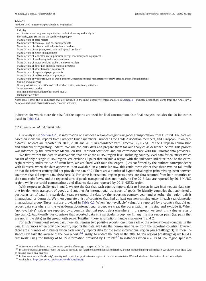
Table C.1Products Used in Input-Output-Weighted Regressions.

IndustryArchitectural and engineering activities; technical testing and analysisElectricity, gas, steam and air conditioning supplyManufacture of basic metalsManufacture of chemicals and chemical productsManufacture of coke and refined petroleum productsManufacture of computer, electronic and optical productsManufacture of electrical equipmentManufacture of fabricated metal products, except machinery and equipmentManufacture of machinery and equipment n.e.c.Manufacture of motor vehicles, trailers and semi-trailersManufacture of other non-metallic mineral productsManufacture of other transport equipmentManufacture of paper and paper productsManufacture of rubber and plastic productsManufacture of wood/products of wood and cork, except furniture; manufacture of straw articles and plaiting materialsMining and quarryingOther professional, scientific and technical activities; veterinary activitiesOther service activitiesPrinting and reproduction of recorded mediaPublishing activities

Note: Table shows the 20 industries that are included in the input-output-weighted analyses in Section 4.1. Industry descriptions come from the NACE Rev. 2European statistical classifications of economic activities.


industries for which more than half of the exports are used for final consumption. Our final analysis includes the 20 industrieslisted in Table C.1.

C.2. Construction of rail freight data

Our analyses in Section 4.2 use information on European region-to-region rail goods transportation from Eurostat. The data arebased on individual reports from European Union members, European Free Trade Association members, and European Union can-didates. The data are reported for 2005, 2010, and 2015, in accordance with Directive 80/1177/EC of the European Commissionand subsequent regulatory updates. We use the 2015 data and prepare them for our analyses as described below. This processwas informed by the “Reference Manual on Rail Transport Statistics” and our correspondence with the Eurostat data providers.

We first restrict the data to observations that are at the NUTS2 region level, including country-level data for countries whichconsist of only a single NUTS2 region. We exclude all pairs that include a region with the unknown indicator “XX” or the extra-regio territory indicator “ZZ”.24 From here, we are faced with four challenges: 1) As confirmed by the authors' correspondencewith Eurostat, when the data appear as “non-available” in a particular row, this could mean either that there was no rail trafficor that the relevant country did not provide the data.25 2) There are a number of hypothetical region pairs missing, even betweencountries that did report data elsewhere. 3) For some international region pairs, there are data reported from both countries onthe same train flows, and the reported tons of goods transported does not match. 4) The 2015 data are reported by 2013 NUTS2region, while our social connectedness and distance data are reported by 2016 NUTS2 region.

With respect to challenges 1 and 2, we use the fact that each country reports data to Eurostat in two intermediate data sets:one for domestic transport of goods and another for international transport of goods. To identify countries that submitted aparticular set of data in a particular year, we group the data by the reporting country, year, and whether the region pair isinternational or domestic. We then generate a list of countries that had at least one non-missing entry in each year/domestic-international group. These lists are provided in Table C.2. When “non-available” values are reported by a country that did notreport data elsewhere in the year/domestic-international group, we treat the observation as missing and exclude it. When“non-available” values are reported by a country that did report data elsewhere in the group, we treat this value as a zero(no traffic). Additionally, for countries that reported data in a particular group, we fill any missing region pairs (i.e. pairs thatare not in the data) in the group with zeros. Together, these assumptions handle challenges 1 and 2.

For each international region pair, there still remain two possible reports: one from each of the regions' home countries in thepair. In instances when only one country reports the data, we take the non-missing value from the reporting country. However,there are a number of instances when each country reports data for the same international region pair (challenge 3). In these in-stances, we take the average of the two reports.26 Finally, to update the data to the 2016 NUTS2 regions (challenge 4) we build acrosswalk using the history of NUTS information provided by Eurostat.27 In instances when a 2013 NUTS2 region split into

24 Observations with these two codes make up 4.9% of tonnage transported in the data.25 In some instances, countries report the data to Eurostat, but flag them as confidential so that they are not included in the public release.We always treat these dataas missing in our final analysis.26 In few instances, a “third-party” country will report transport between regions in two other countries. We exclude these observations from our analysis.27 Available at: https://ec.europa.eu/eurostat/web/nuts/history.

31

https://ec.europa.eu/eurostat/web/nuts/history

Table C.2Rail Freight Data Availability By Reporting Country.

Reporting Domestic International Reporting Domestic International

Country Data Data Country Data DataAlbania N N Lithuania Y YAustria N N Luxembourg Y YBelgium N N Malta N NBulgaria Y Y Montenegro N NCroatia Y Y Netherlands Y NCyprus N N Norway Y YCzech Republic Y Y Poland Y YDenmark Y Y Portugal Y NEstonia Y Y Romania Y NFinland Y Y Serbia N NFrance N N Slovakia Y YGermany Y Y Slovenia Y YGreece N N Spain Y YHungary N N Sweden N NIceland N N Switzerland N NIreland Y Y North Macedonia N NItaly Y Y Turkey Y NLatvia Y Y United Kingdom N NLiechtenstein N N

Note: Table shows the rail goods transportation data availability by reporting country and by type of trade (domestic or international). Y (N) indicates the data are(not) available. The table only shows availability at the reporter level, not whether any regions from this country are included in the final analysis. For example,although Austria did not report international data in 2015, pairs that include an Austrian region and a region in a country that did report international data in 2015are nevertheless included.

Fig. C.1. Randomization inference. Note: Figures show the distribution of regression coefficients for randomly selected values of social connectedness and distance.Panel A shows the coefficients for social connectedness, and Panel B the coefficients for distance. The regression specification is equal to column 4 in Table 3;namely it is a regression of industry-level trade between countries on industry-specific measures of social connectedness and distance. The coefficients obtainedin the original regression are shown as the dashed lines. We contrast the actual estimates with regression coefficients that are obtained when choosing“random” values for social connectedness and distance. To be more precise, for each country i × country j × product p triplet, we assign a value of log(SCIi,jp )and log(Distancei,jp ) from a randomly chosen product in the same country pair. We then estimate a regression based on these “random” values and repeat thisexercise 2000 times. The distribution of estimated coefficients is then plotted in a histogram.


multiple regions, we set the tons of goods transported in each of the 2016 NUTS2 observations equal to the corresponding 2013NUTS2 region tons of goods transported, multiplied by the region's 2015 population share (i.e. we assume that tons of goodstransported in each of these regions is proportional to the 2015 population).

C.3. Randomization inference

An alternative way of exploring the statistical significance of the estimates in column 4 of Table 3 is the following. For eachcountry i × country j × product p triplet, we assign a value of log(SCI i,jp ) and log(Distance i,jp ) from a randomly chosen product

32


in the same country pair, and then re-run the regression. We repeat this exercise 2,000 times. The histograms in Fig. C.1 show thedistribution of the coefficients on the re-shuffled values of input-output-weighted social connectedness and distance; the dashedlines shows the estimated effect corresponding to column 4 of Table 3. The randomized coefficients are centered around zero:conditional on country pair fixed effects, there is no additional explanatory power for trade in a given product coming from var-iation in input-output-weighted social connectedness of a random product. Said differently, what matters is not the social con-nectedness of regions involved in trade generally; instead, what matters for the trade in a specific product is the socialconnectedness across regions that produce and use that specific good.

References

Akcay, Erol, Hirshleifer, David, 2020. Social Transmission Bias and Cultural Evolution in Financial Markets. Technical report. National Bureau of Economic Research.Aker, Jenny C., 2010. Information from markets near and far: Mobile phones and agricultural markets in niger. Am. Econ. J. Appl. Econ. 2 (3), 46–59.Alesina, Alberto, Devleeschauwer, Arnaud, Easterly, William, Kurlat, Sergio, Wacziarg, Romain, 2003. Fractionalization. J. Econ. Growth 8 (2), 155–194.Allen, Treb, 2014. Information frictions in trade. Econometrica 82 (6), 2041–2083.Anderson, James E., Marcouiller, Douglas, 2002. Insecurity and the pattern of trade: an empirical investigation. Rev. Econ. Stat. 84 (2), 342–352.Anderson, James E., Van Wincoop, Eric, 2003. Gravity with gravitas: a solution to the border puzzle. Am. Econ. Rev. 93 (1), 170–192.Bailey, Michael, Cao, Rachel, Kuchler, Theresa, Stroebel, Johannes, Wong, Arlene, 2018a. Social connectedness: measurement, determinants, and effects. J. Econ.

Perspect. 32 (3), 259–280.Bailey, Michael, Cao, Ruiqing, Kuchler, Theresa, Stroebel, Johannes, 2018b. The economic effects of social networks: evidence from the housing market. J. Polit. Econ.

126 (6), 2224–2276.Bailey, Michael, Johnston, Drew M., Kuchler, Theresa, Stroebel, Johannes, Wong, Arlene, 2019a. Peer Effects in Product Adoption. Technical report. National Bureau of

Economic Research.Bailey, Michael, Dávila, Eduardo, Kuchler, Theresa, Stroebel, Johannes, 2019b. House Price Beliefs and Mortgage Leverage Choice. Technical report. 6.Bailey, Michael, Farrell, Patrick, Kuchler, Theresa, Stroebel, Johannes, 2020a. Social connectedness in urban areas. J. Urban Econ. Volume 118, July 2020, 103264.Bailey, Michael, Johnston, Drew, Koenen, Martin, Kuchler, Theresa, Russel, Dominic, Stroebel, Johannes, 2020b. Social Distancing During a Pandemic: The Role of

Friends. Working paper. National Bureau of Economic Research.Bailey, Michael, Johnston, Drew, Kuchler, Theresa, Russel, Dominic, Stroebel, Johannes, et al., 2020c. The determinants of social connectedness in europe. International

Conference on Social Informatics. Springer pages 1–14.Baker, Scott R., 2018. Debt and the response to household income shocks: Validation and application of linked financial account data. J. Polit. Econ. 126 (4), 1504–1557.Bali, Turan G., Hirshleifer, David A., Peng, Lin, Tang, Yi, 2018. Attention, social interaction, and investor attraction to lottery stocks. 9th Miami Behavioral Finance

Conference.Berkowitz, Daniel, Moenius, Johannes, Pistor, Katharina, 2006. Trade, law, and product complexity. Rev. Econ. Stat. 88 (2), 363–373.Bernard, Andrew B., Eaton, Jonathan, Jensen, J. Bradford, Kortum, Samuel, 2003. Plants and productivity in international trade. Am. Econ. Rev. 93 (4), 1268–1290.Bernard, Andrew B., Jensen, J. Bradford, Redding, Stephen J., Schott, Peter K., 2007. Firms in international trade. J. Econ. Perspect. 21 (3), 105–130.Bernard, Andrew B., Jensen, J. Bradford, Redding, Stephen J., Schott, Peter K., 2012. The empirics of firm heterogeneity and international trade. Ann. Rev. Econ. 4 (1),

283–313.Burchardi, Konrad B., Chaney, Thomas, Hassan, Tarek A., 2016. Migrants, Ancestors, and Investments. Technical report. .Chaney, Thomas, 2008. Distorted gravity: the intensive and extensive margins of international trade. Am. Econ. Rev. 98 (4), 1707–1721.Chaney, Thomas, 2014. The network structure of international trade. Am. Econ. Rev. 104 (11), 3600–3634.Chaney, Thomas, 2016. Networks in international trade. The Oxford Handbook of The Economics of Networks.Chaney, Thomas, 2018. The gravity equation in international trade: an explanation. J. Polit. Econ. 126 (1), 150–177.Chen, Natalie, 2004. Intra-national versus international trade in the european union: why do national borders matter? J. Int. Econ. 63 (1), 93–118.Chetty, Raj, Hendren, Nathaniel, Jackson, Matthew O., Kuchler, Theresa, Johannes, et al., Stroebel, 2020. Social Capital in the United States: Measurement, Determinants,

and Associations With Economic Mobility. Working paper. .Combes, Pierre-Philippe, Lafourcade, Miren, Mayer, Thierry, 2005. The trade-creating effects of business and social networks: evidence from France. J. Int. Econ. 66 (1),

1–29.Correia, Sergio, Guimarães, Paulo, Zylkin, Thomas, 2019a. Verifying the Existence of Maximum Likelihood Estimates for Generalized Linear Models.Correia, Sergio, Guimarães, Paulo, Zylkin, Thomas, 2019b. ppmlhdfe: Fast Poisson Estimation With High-Dimensional Fixed Effects.Davis, Kingsley, 1951. The Population of India and Pakistan.Disdier, Anne-Célia, Head, Keith, 2008. The puzzling persistence of the distance effect on bilateral trade. Rev. Econ. Stat. 90 (1), 37–48.Duggan, Maeve, Ellison, Nicole B., Lampe, Cliff, Lenhart, Amanda, Madden, Mary, January 2015. Social Media Update 2014. Pew Research Center.Duggan, Maeve, Greenwood, Shannon, Perrin, Andrew, November 2016. Social Media Update 2016. Pew Research Center.Dunlevy, James A., 2006. The influence of corruption and language on the protrade effect of immigrants: evidence from the american states. Rev. Econ. Stat. 88 (1),

182–186.Eaton, Jonathan, Kortum, Samuel, 2002. Technology, geography, and trade. Econometrica 70 (5), 1741–1779.Einav, Liran, Kuchler, Theresa, Levin, Jonathan, Sundaresan, Neel, 2015. Assessing sale strategies in online markets using matched listings. Am. Econ. J. 7 (2), 215–247.Felbermayr, Gabriel J., Toubal, Farid, 2012. Revisiting the trade-migration nexus: evidence from new oecd data. World Dev. 40 (5), 928–937.Gaulier, Guillaume, Zignago, Soledad, 2010. Baci: International Trade Database at the Product-Level (the 1994–2007 Version).Giglio, Stefano, Maggiori, Matteo, Stroebel, Johannes, Weber, Andreas, 2015. Climate Change and Long-Run Discount Rates: Evidence From Real Estate. Technical

report. .Granovetter, Mark S., 1977. The strength of weak ties. Social Networks. Elsevier pages 347–367.Granovetter, Mark, 2005. The impact of social structure on economic outcomes. J. Econ. Perspect. 19 (1), 33–50.Greif, Avner, 1989. Reputation and coalitions in medieval trade: evidence on the maghribi traders. J. Econ. Hist. 49 (4), 857–882.Greif, Avner, 1993. Contract enforceability and economic institutions in early trade: the maghribi traders' coalition. Am. Econ. Rev. Vol. 83, No. 3 (Jun., 1993),

pp. 525–548 (24 pages).Keith Head and Thierry Mayer. Gravity equations: Workhorse, toolkit, and cookbook. In Handbook of International Economics, 4, pages 131–195. Elsevier, 2014.Helpman, Elhanan, Melitz, Marc, Rubinstein, Yona, 2008. Estimating trade flows: trading partners and trading volumes. Q. J. Econ. 123 (2), 441–487.Hirshleifer, David, 2020. Presidential address: Social transmission bias in economics and finance. J. Financ. 75 (4), 1779–1831.Hirshleifer, David, Lin, Peng, Wang, Qiguang, 2019. Social Interaction and Market Reaction to Earnings News. Technical report, Working Paper. .Hortaçsu, Ali, Martínez-Jerez, F., Douglas, Jason, 2009. The geography of trade in online transactions: Evidence from ebay and mercadolibre. Am. Econ. J. 1 (1), 53–74.Jensen, Robert, 2007. The digital provide: information (technology), market performance, and welfare in the south indian fisheries sector. Q. J. Econ. 122 (3), 879–924.Kaufmann, Daniel, Kraay, Aart, Mastruzzi, Massimo, 2011. Theworldwide governance indicators: methodology and analytical issues. Hague J. Rule Law 3 (2), 220–246.Kuchler, Theresa, Stroebel, Johannes, 2020. Social Finance. Technical report. National Bureau of Economic Research.Kuchler, Theresa, Li, Yan, Lin, Peng, Stroebel, Johannes, Zhou, Dexin, 2020a. Social Proximity to Capital: Implications for Investors and Firms. Technical report. National

Bureau of Economic Research.

33

http://refhub.elsevier.com/S0022-1996(20)30133-1/rf0005

































































Kuchler, Theresa, Russel, Dominic, Stroebel, Johannes, 2020b. The Geographic Spread of Covid-19 Correlates with Structure of Social Networks as Measured byFacebook. Technical report. National Bureau of Economic Research.

Leamer, Edward E., Levinsohn, James, 1995. International trade theory: the evidence. Handbook of International Economics. 3, pp. 1339–1394.Levchenko, Andrei A., 2007. Institutional quality and international trade. The Review of Economic Studies 74 (3), 791–819.Linder, Staffan Burenstam, 1961. An essay on trade and transformation. Almqvist & Wiksell Stockholm.McCallum, John, 1995. National borders matter: Canada-us regional trade patterns. Am. Econ. Rev. 85 (3), 615–623.Melitz, Marc J., 2003. The impact of trade on intra-industry reallocations and aggregate industry productivity. Econometrica 71 (6), 1695–1725.Melitz, Marc J., Ottaviano, Gianmarco I.P., 2008. Market size, trade, and productivity. Rev. Econ. Stud. 75 (1), 295–316.Nunn, Nathan, 2007. Relationship-specificity, incomplete contracts, and the pattern of trade. Q. J. Econ. 122 (2), 569–600.Obstfeld, Maurice, Rogoff, Kenneth, 2000. The six major puzzles in international macroeconomics: is there a common cause? NBER Macroecon. Annu. 15, 339–390.Pemberton, Trevor J., DeGiorgio, Michael, Rosenberg, Noah A., 2013. Population structure in a comprehensive genomic data set on human microsatellite variation. G3

Genes Genom. Genet. 3 (5), 891–907.Piazzesi, Monika, Schneider, Martin, Stroebel, Johannes, 2015. Segmented Housing Search. Technical report. .Ranjan, Priya, Lee, Jae Young, 2007. Contract enforcement and international trade. Econ. Polit. 19 (2), 191–218.Rauch, James E., 1999. Networks versus markets in international trade. J. Int. Econ. 48 (1), 7–35.Rauch, James E., 2001. Business and social networks in international trade. J. Econ. Lit. 39 (4), 1177–1203.Rauch, James E., Trindade, Vitor, 2002. Ethnic chinese networks in international trade. Rev. Econ. Stat. 84 (1), 116–130.Rehbein, Oliver, Rother, Simon, et al., 2020. Distance in Bank Lending: The Role of Social Networks. Technical report. University of Bonn and University of Mannheim,

Germany.Santos Silve, J.M.C., Tenreyro, Silvana, 2006. The log of gravity. Rev. Econ. Stat. 88 (4), 641–658.Simonovska, Ina, Waugh, Michael E., 2014. The elasticity of trade: estimates and evidence. J. Int. Econ. 92 (1), 34–50.Spolaore, Enrico, Wacziarg, Romain, 2016. Ancestry, language and culture. The Palgrave Handbook of Economics and Language. Springer pages 174–211.Spolaore, Enrico, Wacziarg, Romain, 2018. Ancestry and development: new evidence. J. Appl. Econ. 33 (5), 748–762.Startz, Meredith, 2016. The Value of Face-to-Face: Search and Contracting Problems in Nigerian Trade. Working Paper. .Steinwender, Claudia, 2018. Real effects of information frictions: when the states and the kingdom became united. Am. Econ. Rev. 108 (3), 657–696.Tan, Shawn W., 2016. The Geography of Trade in the European Single Market.Timmer, Marcel P., Dietzenbacher, Erik, Los, Bart, Stehrer, Robert, De Vries, Gaaitzen J., 2015. An illustrated user guide to the world input–output database: the case of

global automotive production. Rev. Int. Econ. 23 (3), 575–605.Tinbergen, Jan J., 1962. Shaping the World Economy; Suggestions for an International Economic Policy.Trefler, Daniel, 1995. The case of the missing trade and other mysteries. Am. Econ. Rev. Vol. 85, No. 5 (Dec., 1995), pp. 1029–1046.Wagner, Don, Head, Keith, Ries, John, 2002. Immigration and the trade of provinces. Scottish J. Polit. Econ. 49 (5), 507–525.Wilson, Riley, 2019. The Impact of Social Networks on Eitc Claiming Behavior.

34

































Documents

International trade and social connectedness