International Trade Costs, Global Supply Chains and Value ... · International Trade Costs, Global Supply Chains and Value-added Trade in Australia Gerard Kelly and Gianni La Cava

Research Discussion Paper

International Trade Costs, Global Supply Chains and Value-added Trade in Australia

Gerard Kelly and Gianni La Cava

RDP 2014-07

The Discussion Paper series is intended to make the results of the current economic research within the Reserve Bank available to other economists. Its aim is to present preliminary results of research so as to encourage discussion and comment. Views expressed in this paper are those of the authors and not necessarily those of the Reserve Bank. Use of any results from this paper should clearly attribute the work to the authors and not to the Reserve Bank of Australia.

The contents of this publication shall not be reproduced, sold or distributed without the prior consent of the Reserve Bank of Australia.

ISSN 1320-7229 (Print)

ISSN 1448-5109 (Online)

International Trade Costs, Global Supply Chains andValue-added Trade in Australia


Research Discussion Paper2014-07

August 2014

Economic GroupReserve Bank of Australia

We would like to thank Andrew Cadogan-Cowper, Christian Gillitzer,Alexandra Heath, James Holloway and John Simon for useful comments andsuggestions. The views expressed in this paper are our own and do not necessarilyreflect those of the Reserve Bank of Australia. We are solely responsible for anyerrors.

Authors: kellyg and lacavag at domain rba.gov.au

Media Office: [email protected]

Abstract

We examine how the structure of Australian production and trade has been affectedby the expansion of global production networks. As conventional measures ofinternational trade do not fully capture the impact of global supply chains,we present complementary estimates of value-added trade for Australia. Thesevalue-added trade estimates suggest that the United States and Europe are moreimportant for export demand than implied by conventional trade statistics, assome Australian content is exported to those locations indirectly via east Asia.The estimates also highlight the importance of the services sector to Australiantrade, as the services sector is integral to producing goods exports.

We also find that, compared to thirty years ago, Australian production nowinvolves more stages of production, a greater share of production occurs overseas,and more production occurs towards the start of the supply chain. For Australia,these structural adjustments mainly occurred during the 1990s, and we provideevidence that similar adjustments have occurred elsewhere in the world driven byseveral factors, including lower international trade costs, deregulation of marketsthat produce intermediate goods and services, and economic development inemerging economies, such as China.

JEL Classification Numbers: D57, E01, F12, F60, L16, L23Keywords: fragmentation, supply chains, trade costs, value-added trade

i

Table of Contents

1. Introduction 1

2. The Structure of Australia’s International Trade 2

2.1 Background 2

2.2 Measurement of International Trade 4

2.3 The World Input-Output Database 6

3. Value-added Trade and the Australian Economy 7

3.1 Value-added Trade by Trading Partner 9

3.2 Value-added Trade by Sector 11

3.3 Aggregate Value-added Trade 12

4. The Structure of Australia’s Domestic Supply Chain 14

4.1 Measuring the Domestic Supply Chain 14

4.2 The Domestic Supply Chain in Australia 17

5. Regression Analysis 22

5.1 Hypotheses 22

5.2 International Trade Costs 23

5.3 Domestic Trade Costs and Sectoral Regulation 28

5.4 Modelling Framework 30

5.5 Regression Results 33

6. Conclusion 36

Appendix A: Construction of Value-added Trade Estimates 38

Appendix B: Construction of Supply Chain Statistics 41

Appendix C: Shift-Share Analysis 45

ii

Appendix D: Measures of International Trade Costs 47

Appendix E: Measures of Sectoral Regulation 49

Appendix F: Other Supply Chain Indicators 50

References 52

iii

International Trade Costs, Global Supply Chains andValue-added Trade in Australia


1. Introduction

Structural change in the Australian economy has been a prominent issue in recentyears (Connolly and Lewis 2010). We provide a new perspective on structuralchange by investigating how the domestic supply chain has evolved in recentdecades. We also examine how the structure of Australian international trade hasevolved in response to the development of global supply networks. The paper isdivided into three parts.

First, we investigate how Australian trade has been affected by the growingfragmentation of production across international borders through global supplychains. Australia’s trade linkages have been affected by the expansion of globalproduction networks; Australia typically exports commodities that are used toproduce goods and services that are, in turn, exported to other markets. We presentnew estimates of value-added trade for Australia that complement conventionaltrade statistics. The value-added trade estimates suggest that the United States andEurope are more important for export demand than implied by conventional tradestatistics, as some Australian content is indirectly exported there via east Asia. Thevalue-added trade estimates also highlight the extent to which the services sectoris integral to the production of goods exports.

Second, we quantify how the Australian supply chain has evolved in recentdecades using novel measures based on historical input-output tables. Overall,compared to a few decades ago, the Australian economy now involves more stagesof production, with a greater share of production occuring overseas and moredomestic production occuring earlier in the supply chain. That is, production inthe Australian economy has become more ‘vertically fragmented’, more ‘offshore’and more ‘upstream’. Most of these adjustments occurred over the 1990s, whichsuggests that economic reform and competitive pressures due to ‘globalisation’were contributing factors.

2

Third, we undertake econometric analysis to explore how the level of verticalfragmentation across countries and industries has been affected by factors suchas lower international trade costs and deregulation of product markets.

2. The Structure of Australia’s International Trade

2.1 Background

The structure of international trade has changed dramatically in recent decades. Akey feature of this structural change has been the increasing role of global supplychains. Global supply (or value) chains are production networks that span multiplecountries, with at least one country importing inputs and exporting output. Theproduction of a single good, such as a mobile phone or television, typically nowtakes place across several countries, with each country specialising in a particularphase or component of the final product (Riad et al 2012).

International trade has risen, as a share of world GDP, from less than 20 per cent inthe mid 1990s to more than 25 per cent more recently (Figure 1). More notably, thegrowth in trade has been dominated by trade in intermediate inputs – goods andservices that are not consumed directly but are used to produce other goods andservices.1 The rapid growth in trade in intermediate inputs has been facilitated byfactors that have lowered the cost of trade, such as: advances in transportation andcommunication technologies; the liberalisation of trade; the removal of foreigncapital controls; and the growing industrial capacity of emerging economies.2

A related feature of this structural change in recent decades has been the growthin intraregional trade and the emergence of regional supply networks. This hasbeen particularly apparent in east Asia where a regional supply network hasdeveloped that specialises in producing components for computers and otherelectronic devices (Craig, Elias and Noone 2011). China has played a central

1 The concept of trade in intermediate inputs (or ‘supply-chain trade’) is closely related to thenotion of ‘intra-industry trade’ (Baldwin and Lopez-Gonzalez 2013). However, we focus onsupply-chain trade as we believe it is a broader concept that encompasses both inter-industryand intra-industry trade.

2 Some of the trend increase in the value of intermediate exports relative to GDP over the midto late 2000s is due to a relative price increase and, in particular, the rise in world commodityprices.

3

Figure 1: World ExportsCurrent prices, per cent of GDP

1995 1999 2003 2007 20116

8

10

12

14

16

18

20

6

8

10

12

14

16

18

20

Final

%%

Intermediate

Source: World Input-Output Database

role in the development of this supply network, following its accession to theWorld Trade Organization (WTO) in 2001. China has experienced large inflows offoreign direct investment and has become a major destination for the outsourcingand offshoring of global manufacturing. It is now a core market for intermediateproducts, such as resource commodities from Australia and complex manufacturedcomponents from Asian countries. These intermediate products are used toproduce final goods, many of which are exported to advanced economies.

The growing prevalence of global supply chains, and the related rise of tradein intermediate inputs, has a direct bearing on the structure of Australian trade.Australian exports of intermediate goods and services have consistently exceededexports of final goods and services over the past two decades (left-hand panel ofFigure 2). Moreover, the gap between the two types of trade has widened overrecent years. This reflects the resource boom, as a significant share of Australia’sresource commodities are exported to east Asia where they are used to producegoods and services that are either sold within east Asia or re-exported to otherparts of the world. Australia’s growing integration into global supply networks isillustrated by the fact that Australia is increasingly a net exporter of intermediate

4

Figure 2: Australia – TradeCurrent prices, per cent of GDP

0

3

6

9

12

15

Intermediate

%Exports

-9

-6

-3

0

3

6

2013

Net exports

Final

20051997201320051997

%

Sources: ABS; Authors’ calculations

goods and services, and a net importer of final goods and services (right-handpanel of Figure 2).3

2.2 Measurement of International Trade

Conventional measures of international trade based on gross flows of exports andimports do not fully capture the impact of global supply chains on Australian trade.We construct estimates of ‘value-added trade’, which complement conventionalmeasures, and illustrate how the fragmentation of production across internationalborders has affected Australian trade. Unlike conventional trade statistics, value-added trade statistics identify the contributions of each country and each industryto the final value of an exported good or service. While conventional trade statisticsidentify the initial destination of a country’s exports, value-added measuresidentify both the initial and effective final export destinations. A comparison of

3 The rise in the value of net exports of intermediate goods and services (relative to GDP) overrecent years is also partly due to higher prices for Australia’s commodity exports, such as ironore and coal.

5

gross trade and value-added trade statistics provides a guide to the extent to whichdemand shocks stemming from final export destinations indirectly affect Australia.

Conventional trade statistics typically measure the value of goods and serviceseach time they cross a border. These estimates form the basis of internationaltrade measured in the national accounts and balance of payments and are the mostreliable and timely source of information on imports and exports. But gross tradeflows do not necessarily identify the countries and industries that contribute to theproduction of the traded good or service; instead, the full value is attributed to thelast country and industry that shipped the product. A component of an exportedgood that crosses international borders multiple times in the process of becoming afinished good is counted multiple times under conventional measures. As a result,gross measures of trade flows can inflate the amount of trade (relative to domesticoutput) and provide a distorted view of a country’s bilateral trade flows.

These measures of trade reflect the way in which economic activity is measuredwithin and across national borders. GDP, the most commonly used indicator ofa nation’s domestic economic activity, records only expenditures on final goodsand services (or ‘final demand’) and excludes expenditures on intermediate goodsand services (or ‘intermediate consumption’). GDP therefore measures the value-added in the production process. For example, suppose an iron ore miner producesiron ore worth $100 (without any intermediate inputs) and sells it to anotherfirm, which uses the iron ore as an intermediate input to produce a refrigerator,which is then sold domestically as a finished good for $110. The ‘gross output’of the economy is equal to $210, while the ‘value-added’ (as measured by finalexpenditure) is equal to $110. The national accounts will record the ‘value-added’of the finished good ($110) as GDP, effectively avoiding counting the value ofintermediate inputs multiple times.

To take a similar example, consider the trade flows depicted in Figure 3. Supposethe iron ore producer exports the iron ore, produced entirely within Australia,worth $100 to a firm in China. The firm in China then processes the ironore (adding value of $10) to create a refrigerator which is exported to theUnited States, where it is sold as a finished good (for a full value of $110).The conventional measure of trade would record total global exports and importsof $210, despite only $110 of value-added being generated in production. Theconventional measure would show that the United States has a trade deficit of

6

$110 with China, and no trade at all with Australia, despite Australia being thechief beneficiary of the final demand of the United States. If, instead, the tradeflows were measured in value-added terms, total trade would equal $110. Also,the trade deficit of the United States with China would be only $10, and it wouldrun a deficit of $100 with Australia.

Figure 3: Comparison of Gross Trade and Value-added Trade

$10

$210 total $110 total

Gross trade Value-added trade

China(+ 10)

Australia(+ 100)

US(– 110)

China(+ 10)

Australia(+ 100)

US(– 110)

$100

$110$100

This example highlights the two main issues with the conventional measurementapproach: gross trade provides an upper-bound estimate of the contribution oftrade to economic activity, and the composition of each country’s trade balancedoes not necessarily reflect value-added trade flows. However, while bilateralgross and value-added trade balances can differ, the aggregate level of eachcountry’s trade balance is the same when measured in either gross or value-addedterms. In the example, Australia has an aggregate surplus of $100, China has anaggregate surplus of $10, and the United States has an aggregate deficit of $110under either approach to measuring international trade.

2.3 The World Input-Output Database

In recognition of these problems, an alternative measure of trade known as ‘value-added trade’ has recently been developed (Johnson and Noguera 2012). Themeasurement of value-added trade requires very detailed information on howexports and imports are used as intermediate inputs by various countries andindustries. The World Input-Output Database (WIOD) combines information fromnational input-output databases with bilateral trade data to construct harmonisedannual world input-output tables for 35 industries in 40 countries over the period

7

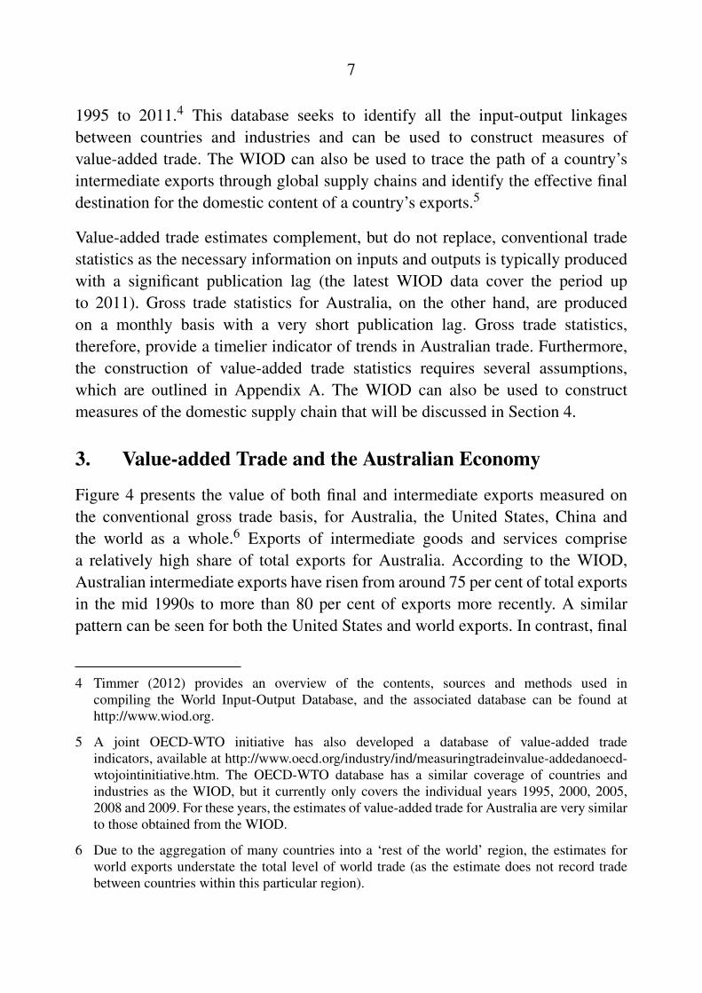
1995 to 2011.4 This database seeks to identify all the input-output linkagesbetween countries and industries and can be used to construct measures ofvalue-added trade. The WIOD can also be used to trace the path of a country’sintermediate exports through global supply chains and identify the effective finaldestination for the domestic content of a country’s exports.5

Value-added trade estimates complement, but do not replace, conventional tradestatistics as the necessary information on inputs and outputs is typically producedwith a significant publication lag (the latest WIOD data cover the period upto 2011). Gross trade statistics for Australia, on the other hand, are producedon a monthly basis with a very short publication lag. Gross trade statistics,therefore, provide a timelier indicator of trends in Australian trade. Furthermore,the construction of value-added trade statistics requires several assumptions,which are outlined in Appendix A. The WIOD can also be used to constructmeasures of the domestic supply chain that will be discussed in Section 4.

3. Value-added Trade and the Australian Economy

Figure 4 presents the value of both final and intermediate exports measured onthe conventional gross trade basis, for Australia, the United States, China andthe world as a whole.6 Exports of intermediate goods and services comprisea relatively high share of total exports for Australia. According to the WIOD,Australian intermediate exports have risen from around 75 per cent of total exportsin the mid 1990s to more than 80 per cent of exports more recently. A similarpattern can be seen for both the United States and world exports. In contrast, final

4 Timmer (2012) provides an overview of the contents, sources and methods used incompiling the World Input-Output Database, and the associated database can be found athttp://www.wiod.org.

5 A joint OECD-WTO initiative has also developed a database of value-added tradeindicators, available at http://www.oecd.org/industry/ind/measuringtradeinvalue-addedanoecd-wtojointinitiative.htm. The OECD-WTO database has a similar coverage of countries andindustries as the WIOD, but it currently only covers the individual years 1995, 2000, 2005,2008 and 2009. For these years, the estimates of value-added trade for Australia are very similarto those obtained from the WIOD.

6 Due to the aggregation of many countries into a ‘rest of the world’ region, the estimates forworld exports understate the total level of world trade (as the estimate does not record tradebetween countries within this particular region).

8

goods and services comprise a much higher share of Chinese exports, reflectingChina’s role as an assembly point in many global supply chains.

Figure 4: Gross Exports

100

200

300

■ Intermediate ■ Final

Australia US

China World

US$b

US$b

US$b

US$b

1 500

1 000

500

1999 2005 20110

750

1 500

2 250

1999 2005 2011

10 000

5 000

15 000

0

Source: World Input-Output Database

To compare estimates of value-added trade with conventional estimates of grosstrade, it is useful to construct a summary indicator known as the ‘VAX ratio’(Johnson and Noguera 2012). This is the ratio of value-added exports to grossexports and is an approximate measure of the domestic value-added content ofexports. The VAX ratio can be constructed for each bilateral trading pair or eachindustry of a given country. By definition, the bilateral VAX ratio is less thanone when value-added exports are less than gross exports, which can occur eitherbecause some of the value of the exports is imported from another country orbecause the trading partner re-exports the content to another destination. Thebilateral VAX ratio is greater than one when value-added exports exceed grossexports. This can occur when some of the country’s exports reach the tradingpartner directly (as measured by gross exports) and the rest indirectly (whendomestic value-added is embodied in a third country’s exports to that partner). Asimilar logic applies for understanding variation in the measured VAX ratio acrossindividual sectors of the economy. The VAX ratio for a sector can be greater thanone if the sector contributes more as an intermediate input to the value of exports

9

of other sectors than those sectors contribute to the value of its own exports.Conversely, the VAX ratio for a sector can be less than one if intermediate inputsfrom other sectors, or from imports, contribute more to the value of the sector’sexports than it contributes to the exports of other sectors.7

3.1 Value-added Trade by Trading Partner

In terms of trading partners, the main difference between Australia’s grossand value-added exports is the importance of emerging economies relative tothe advanced economies. According to the WIOD, between 2002 and 2011,North America and Europe accounted for 23 per cent of Australia’s gross exports,but about 32 per cent of value-added exports as some Australian production isexported to the advanced economies indirectly via supply chains in Asia (Table 1).Conversely, exports to China, Indonesia, Korea and Taiwan together accounted foronly about 25 per cent of Australia’s value-added exports, but around 32 per centof gross exports, as some of the exports to Asia are used as intermediate inputs toproduce final goods and services that are re-exported to other countries.8

Looking at how the bilateral VAX ratios have evolved over time, there has been asteady increase in the value-added content of Australia’s trade with North Americaand Europe but a gradual decline in the value-added content of Australia’s tradewith east Asia (Figure 5). The volume of both gross and value-added exports toeast Asia, and particularly China, has grown markedly, but an increasing share ofAustralian exports to the region is processed and re-exported rather than consumeddomestically, which has caused the VAX ratio to trend down. These trends mainlyreflect the increasing integration of east Asia into global value chains; the effect isparticularly pronounced during the 2000s.

7 A country’s total value-added trade cannot exceed its gross trade, which implies that the overallVAX ratio cannot be greater than one; only bilateral (or sectoral) value-added trade can exceedgross trade.

8 These estimates assume that, for each industry, the import content of production is the same forexported and non-exported products. But, due to China’s use of export-processing trade zones,Chinese exports tend to have higher imported content than goods and services produced fordomestic consumption. This implies that the WIOD estimates may overstate China’s share ofAustralian value-added exports.

10

Table 1: Australian Exports by Trading Partner2002–2011 average

Trading Share of Share of Difference VAXpartner gross exports value-added Per cent ratio

exportsNorth America 10.3 15.8 5.6 1.27Europe 12.3 15.7 3.4 1.05Japan 15.6 15.0 –0.5 0.79China 17.9 15.0 –2.9 0.70South Korea and Taiwan 11.4 7.6 –3.8 0.54Other trading regions 32.5 30.8 –1.7 0.79Total 100.0 100.0 0.0 0.82Source: World Input-Output Database

Figure 5: Australia – VAX Ratio by Destination

0.2

0.6

1.0

1.4

0.2

0.6

1.0

1.4

2011

ratio

North America

ratio

Europe

JapanChina

South Korea and Taiwan

2007200319991995

Sources: Authors’ calculations; World Input-Output Database

11

3.2 Value-added Trade by Sector

The sectoral mix of Australia’s trade is also different when measured in value-added rather than gross terms (Table 2).9 The sectoral breakdown of Australianexports in value-added terms indicates which sectors ultimately benefit from trade.

Table 2: Value-added Trade by Sector2002–2011 average

Sector Share of Share of Difference VAXgross exports value-added Per cent ratio

exportsManufacturing 37.6 18.9 –18.7 0.41Resources 39.9 37.2 –2.7 0.77Construction and utilities 0.2 3.1 2.9 11.93Services 22.3 40.8 18.5 1.51Total 100.0 100.0 0.0 0.82Source: World Input-Output Database

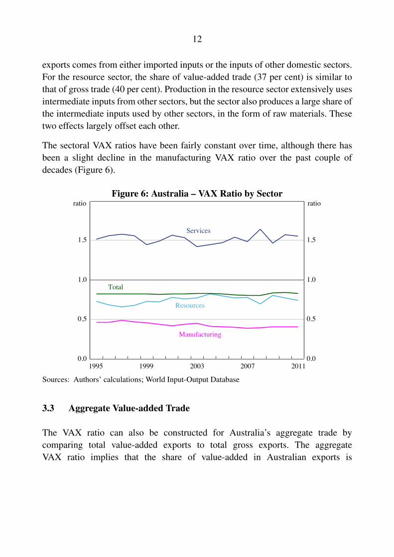
Services exports account for a much higher share of Australia’s exports in value-added terms (41 per cent) than in gross terms (22 per cent) (Table 2). Australia’sexports, therefore, embody a higher share of services than conventionallymeasured. Most services are non-tradeable so the service sector produces asmall share of direct exports as captured by the gross trade statistics. However,services are used extensively as inputs to produce manufactured and resourceexports. For example, services, such as marketing and distribution, account fora relatively large share of the final value of manufactured goods. Furthermore,service industries tend to be labour intensive, requiring relatively few intermediateinputs in their own production.

Conversely, the manufacturing sector comprises a much smaller share of value-added trade (19 per cent) than of gross trade (38 per cent) (Table 2). Theseestimates indicate that about half of the value-added in Australia’s manufacturing

9 The WIOD classification of industries is very similar to that of the 2-digit Australian andNew Zealand Standard Industrial Classification (ANZSIC) system, which is used by theAustralian Bureau of Statistics (ABS). Australian gross exports of resources and manufacturedgoods are slightly higher, on average, based on the WIOD measure compared with the ABSmeasure, but these differences are unlikely to have a significant effect on the sectoral VAXratios. Reclassifying industries into the manufacturing and resources sectors based on the splitused by Rayner and Bishop (2013) has little effect on the measured VAX ratios.

12

exports comes from either imported inputs or the inputs of other domestic sectors.For the resource sector, the share of value-added trade (37 per cent) is similar tothat of gross trade (40 per cent). Production in the resource sector extensively usesintermediate inputs from other sectors, but the sector also produces a large share ofthe intermediate inputs used by other sectors, in the form of raw materials. Thesetwo effects largely offset each other.

The sectoral VAX ratios have been fairly constant over time, although there hasbeen a slight decline in the manufacturing VAX ratio over the past couple ofdecades (Figure 6).

Figure 6: Australia – VAX Ratio by Sector

0.0

0.5

1.0

1.5

0.0

0.5

1.0

1.5

2011

Services

ratio

Manufacturing

Resources

Total

200720031999

ratio

1995


3.3 Aggregate Value-added Trade

The VAX ratio can also be constructed for Australia’s aggregate trade bycomparing total value-added exports to total gross exports. The aggregateVAX ratio implies that the share of value-added in Australian exports is

13

about 82 per cent (Figure 7).10 This is relatively high by international standards;the share of value-added in world exports is about 69 per cent. The high shareof value-added content in Australia’s trade mainly reflects two factors – thecountry’s geographic isolation and its large endowment of natural resources. First,Australia’s geographic isolation means that it is rarely involved in the intermediateprocessing stages of most global supply chains.11 Second, the export of naturalresources requires few imported inputs so the high share of resources in Australia’sexport base implies that most of the value-added of Australian exports is dueto domestic production. In contrast, the value-added content of trade is typicallylow for countries close to production hubs that are heavily involved in productionsharing, such as those in east Asia, Europe and North America. These factors alsolargely explain why the value-added content of Australian trade has declined bymuch less than it has for most other countries since the mid 1990s.12

10 Total value-added exports are not simply the domestic content of total gross exports, but theamount of domestic content that is ultimately consumed as final demand outside the country.Value-added exports exclude ‘reflected exports’, that is, the estimates exclude domestic contentthat is processed outside the country and then imported (e.g. Australia importing a Japanesecar that contains Australian iron ore). But reflected exports represent only a small share ofAustralia’s overall trade, so the VAX ratio provides a reasonable guide to the proportion ofdomestic content in overall exports.

11 These factors also contribute to the country’s relatively low level of trade as a share of GDP(Guttmann and Richards 2004).

12 The VAX ratio is measured in nominal terms and can, therefore, be affected by changes in theprices of intermediate inputs and gross outputs. For example, there is a clear downward spike inthe aggregate VAX ratios of most countries in 2008. This pattern is, at least in part, due to largefluctuations in commodity prices around that time. For instance, commodity prices rose sharplyin 2008, which would have boosted the relative price of intermediate inputs, and reduced thevalue-added content of exports for most countries and industries.

14

Figure 7: Aggregate VAX Ratios

0.4

0.5

0.6

0.7

0.8

0.4

0.5

0.6

0.7

0.8

2011

ratio

Australia

ratio

G7

World

China

South Korea and Taiwan

2007200319991995


4. The Structure of Australia’s Domestic Supply Chain

4.1 Measuring the Domestic Supply Chain

The fragmentation of production across firms and industries within the domesticeconomy has also been an important feature of structural change in Australia.To the best of our knowledge, there has been no research into the structure andevolution of the domestic supply chain in Australia.

Ideally, to measure changes in the structure of the Australian supply chain wewould have information on transactions at the plant-level between buyers andsuppliers. Unfortunately, these data are not available for Australia. Nonetheless,we can extract useful information on the length of supply chains and an industry’sposition along a supply chain from industry-level input-output tables.

The most conventional measure of inter-industry linkages and supply chains isthe ratio of intermediate consumption to gross output. As mentioned earlier, grossoutput is the total market value of goods and services produced in an economy,which can be divided into value-added and the cost of intermediate inputs (or

15

intermediate consumption). Value-added reflects the returns to labour and capitalused by the industry. The higher the share of output that is accounted for byintermediate consumption, the more of the industry’s value is added outside ofthe industry. A high share of intermediate consumption indicates that productionin the industry is ‘vertically fragmented’.

While the ratio of intermediate consumption to gross output is easily estimated,it does not account for the full complexity of inter-industry linkages involved inproduction, nor the length of the supply chain between a good’s production andits consumption. More sophisticated measures have been developed to describethe relative position of an industry in the value-added chain – ‘fragmentation’ and‘upstreamness’ (Fally 2012).

The ‘fragmentation’ statistic measures the number of stages involved in theproduction of a good or service and how the overall value-added of the productis distributed along these stages. Fragmentation is calculated using a good orservice’s inputs. Fragmentation is defined as one plus a weighted sum of thenumber of stages involved in the production of good i’s intermediate inputs, wherethe weight corresponds to the value added by each input. The index takes the valueof one if there is a single production stage in the final industry and increases withthe length of the production chain.

For example, if half of the value of industry A’s gross output is accounted forby intermediate inputs from industry B, and the inputs from industry B do notrequire any inputs themselves, then the ‘fragmentation’ measure of industry Awill be 1 + 0.5 = 1.5. If, however, half of the value of industry B’s output isspent on intermediate inputs from industry C (which themselves do not requireany intermediate inputs) then the fragmentation measure of industry A will be1+0.5× (1+0.5) = 1.75.

An industry’s supply chain will, therefore, be more (or less) fragmented dependingon the extent to which the production of its final output depends on intermediategoods which are themselves more (or less) fragmented. Low fragmentation doesnot necessarily mean a ‘short’ supply chain, but could indicate that the bulk ofvalue-added is concentrated at only one or two stages of a long supply-chain,rather than being dispersed across the length of the chain.

16

The fragmentation measure is mathematically comparable to the measure of totalbackward linkages of a sector in traditional input-output theory, first proposedin the late 1950s and equivalent to measures of sector-to-economy ‘outputmultipliers’ (Miller and Blair 2009). The interpretation of fragmentation as asector’s weighted average number of production stages clarifies the definitionof backward linkages, while avoiding the shortcomings of the ‘multiplier’interpretation.13

The ‘upstreamness’ statistic measures the average number of stages occurringbetween production and final demand of a good or service. Upstreamness iscalculated using the good or service’s outputs. It is defined as one plus a weightedsum of the number of stages between production of the goods that take outputfrom industry i as an input and these goods’ own final demand, where the weightcorresponds to the fraction of industry i’s total production going to each use.

For example, if half of the gross output of industry A is used for final consumptionand half is used as intermediate inputs by industry B, which produces entirelyfor final consumption, then the measured upstreamness of industry A will be1+0.5 = 1.5. If, however, only half of the value of industry B’s output is used forfinal consumption, with the other half used as intermediate inputs by industry C(which produces entirely for final consumption), then the upstreamness measureof industry A will be 1+0.5× (1+0.5) = 1.75.

Industries with low measured upstreamness produce largely for final consumption.An industry that mainly produces for intermediate use will be more upstream,particularly if it produces for other industries that are also upstream.14 Themeasurement of fragmentation and upstreamness requires detailed input-outputdata, giving the relative values of the intermediate inputs that each industryrequires for production. We use a combination of ABS input-output tables and

13 For details on these inherent problems in deriving sector-to-economy output multipliers frominput-output tables see Gretton (2013).

14 The upstreamness measure is mathematically comparable to the measure of total forwardlinkages of a sector in traditional input-output theory (see Jones (1976)), which have also beeninterpreted as ‘supply-driven’ or ‘cost-push’ multipliers, as opposed to the ‘demand-driven’multipliers which are mathematically related to the fragmentation measure (see Miller andBlair (2009)). Antras et al (2012) show how an equivalent measure of distance to final demandcan be reached using an alternative derivation.

17

the WIOD to estimate the supply chain statistics. The calculations are explainedin Appendix B.

4.2 The Domestic Supply Chain in Australia

The two supply chain measures indicate that the Australian domestic supply chaininvolves about two stages of production, on average, and most of this productionoccurs two stages away from final demand. However, there is significant variationin the degree of vertical fragmentation and upstreamness across different sectorsof the economy (Table 3). The manufacturing, construction and utilities sectorstend to be the most fragmented, while the resource sector is the most upstream.In contrast, the services sector tends to be the least fragmented and mostdownstream.15

Table 3: Fragmentation and Upstreamness by Sector2000–2010 average

Sector Fragmentation UpstreamnessManufacturing 2.6 2.5Resources 2.0 3.6Construction and utilities 2.6 1.9Services 1.9 1.9Total 2.1 2.2Source: ABS

This can be seen even more clearly if we decompose these sectoral estimatesand examine the variation in fragmentation and upstreamness across individualindustries (Table 4). The most fragmented industries tend to have long supplychains along which little value-added occurs at each stage. The most fragmentedindustries are typically in the manufacturing sector, including meat, dairy andbasic metals manufacturing. In contrast, the least fragmented industries aretypically services industries, such as education, finance and insurance, and healthand community services.

15 The estimated level of fragmentation and upstreamness across sectors is somewhat sensitiveto the level of sectoral aggregation used in the calculations. However, the estimated trendsfor fragmentation and upstreamness are little affected when we calculate each statistic basedon different degrees of sectoral aggregation. See Appendix B for more details on the issue ofaggregation.

18

The most upstream industries are typically in the resource sector, although theproperty and business services industry is quite upstream too. Manufacturingindustries that produce mainly primary commodities, such as basic metals, alsooccupy very upstream positions. In contrast, the most downstream industries aregenerally in the service sector, such as education, health and community services,and retail trade. Some manufacturing industries, such as motor vehicles andclothing, are also downstream.

Table 4: Industry Ranking of Fragmentation and Upstreamness2009/10

Rank Highest LowestFragmentation

1 Basic metals Finance and insurance2 Meat and dairy Education3 Other food Health and community services4 Transport equipment Personal and other services5 Construction Mining

Upstreamness1 Mining Health and community services2 Basic metals Education3 Forestry and fishing Personal and other services4 Property and business services Public administration5 Non-metallic minerals Retail tradeSource: ABS

We can construct time-series indicators of the domestic supply chain for theaggregate economy using historical input-output tables at roughly three-yearintervals back to the mid 1970s. These supply chain indicators suggest that theAustralian economy has become more fragmented and more upstream sincethe 1970s (Figure 8), while there was a notable increase in both measures overthe 1990s.16 Methodological changes to the input-output tables by the ABS appear

16 These longer-run trends for the Australian economy are in stark contrast to those of theUnited States; the US economy has become progressively less fragmented and less upstreamover the same period (Antras et al 2012; Fally 2012). Fally attributes this to a shift towards amore service-oriented, and hence downstream, economy.

19

to explain at least some of this ‘jump’.17 Given this, for much of the subsequentanalysis, we focus on the WIOD data and the period since the mid 1990s. This isalso the period for which we have comparable international data.

Figure 8: Aggregate Supply Chain Indicators

1975 1987 1995 2006 20101.8

1.9

2.0

2.1

2.2

1.8

1.9

2.0

2.1

2.2

Gross output tovalue-added ratio

index

Upstreamness

Fragmentation

index


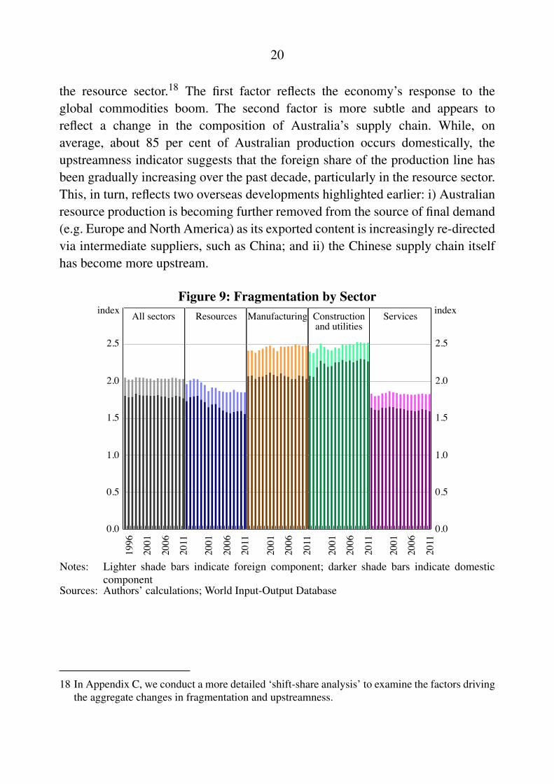
The WIOD data also indicate that, for the Australian economy in aggregate,the degree of fragmentation has been relatively unchanged over the past decade(Figure 9) while the extent of upstreamness has increased (Figure 10). Theincrease in aggregate upstreamness reflects two factors: i) an increase in thevalue of aggregate output accounted for by the resource sector (which is themost upstream sector) and ii) an increase in the level of upstreamness within

17 The ABS input-output tables are constructed from supply and use (S-U) tables, which detailindustries’ production and uses of goods and services and are compiled as part of the AustralianSystem of National Accounts (SNA). While past S-U tables are revised for all periods whenhistorical revisions are made (like other national accounts measures such as GDP), previouslypublished input-output tables are not revised, and therefore do not form a consistent time series.Significant methodological changes were undertaken in the 1990s, including those associatedwith the implementation of SNA93. For details, see Gretton (2005) and Australian Bureau ofStatistics (2013).

20

the resource sector.18 The first factor reflects the economy’s response to theglobal commodities boom. The second factor is more subtle and appears toreflect a change in the composition of Australia’s supply chain. While, onaverage, about 85 per cent of Australian production occurs domestically, theupstreamness indicator suggests that the foreign share of the production line hasbeen gradually increasing over the past decade, particularly in the resource sector.This, in turn, reflects two overseas developments highlighted earlier: i) Australianresource production is becoming further removed from the source of final demand(e.g. Europe and North America) as its exported content is increasingly re-directedvia intermediate suppliers, such as China; and ii) the Chinese supply chain itselfhas become more upstream.

Figure 9: Fragmentation by Sector

1996

2001

2006

2011

0.0

0.5

1.0

1.5

2.0

2.5

2001

2006

2011

2001

2006

2011

0.0

0.5

1.0

1.5

2.0

2.5

indexManufacturing

2001

2006

2011

2001

2006

2011

index Constructionand utilities

ServicesResourcesAll sectors

Notes: Lighter shade bars indicate foreign component; darker shade bars indicate domesticcomponent


18 In Appendix C, we conduct a more detailed ‘shift-share analysis’ to examine the factors drivingthe aggregate changes in fragmentation and upstreamness.

21

Figure 10: Upstreamness by Sector

1996

2001

2006

2011

0.0

0.5

1.0

1.5

2.0

2.5

3.0

3.5

2001

2006

2011

2001

2006

2011

0.0

0.5

1.0

1.5

2.0

2.5

3.0

3.5

indexManufacturing

2001

2006

2011

2001

2006

2011

index Constructionand utilities

ServicesResourcesAll sectors

Notes: Lighter shade bars indicate foreign component; darker shade bars indicate domesticcomponent


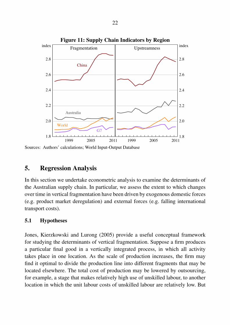
International comparisons based on the WIOD data allow us to put theAustralian estimates into context. Australia’s degree of vertical fragmentation andupstreamness is higher than in the rest of the world, on average (Figure 11).This is particularly true in terms of upstreamness due to Australia’s relativelylarge resource sector. In contrast, the supply chains of the G7 countries tend tobe relatively downstream and less fragmented by international standards. Clearly,China stands out in international comparisons as a country that has a particularlylong and upstream aggregate supply chain.

In fact, Australia has bucked a global upward trend of rising fragmentationsince the early 2000s (left-hand panel, Figure 11). This increase in fragmentationaround the world has been particularly pronounced in the emerging economies andespecially China. On the other hand, the WIOD estimates imply that the degree ofupstreamness has risen in Australia over the past decade at about the same rate asthe world average, and much less quickly than in China.

22

Figure 11: Supply Chain Indicators by Region

1999 2005 20111.8

2.0

2.2

2.4

2.6

2.8China

index

1999 2005 20111.8

2.0

2.2

2.4

2.6

2.8

Fragmentation

Australia

WorldG7

Upstreamness index


5. Regression Analysis

In this section we undertake econometric analysis to examine the determinants ofthe Australian supply chain. In particular, we assess the extent to which changesover time in vertical fragmentation have been driven by exogenous domestic forces(e.g. product market deregulation) and external forces (e.g. falling internationaltransport costs).

5.1 Hypotheses

Jones, Kierzkowski and Lurong (2005) provide a useful conceptual frameworkfor studying the determinants of vertical fragmentation. Suppose a firm producesa particular final good in a vertically integrated process, in which all activitytakes place in one location. As the scale of production increases, the firm mayfind it optimal to divide the production line into different fragments that may belocated elsewhere. The total cost of production may be lowered by outsourcing,for example, a stage that makes relatively high use of unskilled labour, to anotherlocation in which the unit labour costs of unskilled labour are relatively low. But

23

the fragmentation of production is costly as it also requires services that link eachproduction stage, such as transportation and communication activities.

In this framework, it is optimal for the firm to fragment production if thelower costs due to shifting resources to locations with relatively low unitlabour costs outweigh the higher costs associated with the greater service linkactivities. For a graphical exposition of the model and more detailed analysis, seeJones et al (2005).

From this simple model we can derive three testable hypotheses:19

1. Fragmentation rises as an industry (or economy) grows

2. Fragmentation rises as trade (or service link) costs fall

3. Offshoring (or the share of production that occurs in other countries) rises asinternational trade costs fall.

Clearly, information on international and domestic trade costs is required to testthese hypotheses. Before turning to the regression framework, we therefore needto briefly discuss how we measure international and domestic trade costs.

5.2 International Trade Costs

Trade costs can be inferred from an economic model linking trade flows toobservable variables and unobserved trade costs. The standard model in theinternational macroeconomic literature is the ‘gravity model’. This model assumesthat the level of bilateral trade between an importing country and an exportingcountry is a function of the level of economic activity in each of the two countries,as well as bilateral trade barriers. We follow the recent literature by estimatinginternational trade using the inverse gravity model, which essentially ‘flips’ the

19 In essence, there are three key assumptions in the model that generate increasing returns toscale in production and, in turn, deliver the three stated hypotheses. First, there is constantreturns to scale (and hence constant marginal costs) within each production fragment. Second,the fragments vary in terms of factor endowments and productivities, such that marginal costsare lower in some fragments than in others. Third, the costs of services to link different stagesof production mainly comprise fixed costs, so that service link costs do not rise in proportion tooutput.

24

gravity model on its head (Novy 2013). International trade costs can be derivedfrom a micro-founded gravity equation (Anderson and van Wincoop 2003):

xsi jt = (

ysit× ys

jt

yswt

)× (τ

si jt

Psit×Ps

jt)(1−σ

s) (1)

where, for each industry s in year t, xsi jt denotes nominal exports from country i to

country j, ysit and ys

jt denote the levels of output produced in country i and country jrespectively, ysw

t denotes world output, Psit and Ps

jt are the aggregate price indicesof country i and country j respectively, τ

si jt is the bilateral trade cost, σ

s > 1 is theelasticity of substitution across goods within the industry.

Algebraic manipulation of Equation (1) (provided in Appendix D) gives anexpression for international trade costs (θ s

i jt) as a function of bilateral internationaltrade, domestic (or intra-national) trade and the elasticity of substitution inconsumption between goods:

θsi jt = (

τsi jt× τ

sjit

τsiit× τ

sj jt)

12 = (

xsiit× xs

j jt

xsi jt× xs

jit)

12(σs−1) . (2)

The definition of international trade costs combines the ratio of domestic tobilateral trade with an exponent that involves the industry-specific elasticity ofsubstitution. In an industry with highly elastic goods, consumers are very sensitiveto variations in price and so a small price rise induced by bilateral trade costs canlead to a high ratio of domestic to bilateral trade. Therefore, the ratio reflects notonly bilateral trade frictions but also the extent of product differentiation.

The implied estimates of international trade costs include all the costs involvedin moving goods between two countries relative to the cost of selling the goodsdomestically. These trade costs include factors such as transportation costs, policybarriers, information costs, contract enforcement costs, and local distributioncosts. The more two countries trade with each other, the lower is the measureof relative trade costs, all other things being equal.

To compute trade costs across industries, countries and time, we need data onthe bilateral export flows between countries i and j as well as the domestic tradewithin each country. For each industry and year, the domestic trade of each country

25

is assumed to be given by the level of gross output minus total exports to the restof the world. These data are readily available in the WIOD.

As Equation (2) suggests, the trade cost measures also require an estimate of theelasticity of substitution between goods within each industry. We follow Andersonand van Wincoop (2004) and Novy (2013) in setting the elasticity of substitutionequal to eight across all industries and countries. The estimated level of trade costsis very sensitive to this choice of elasticity. However, because the elasticity doesnot vary with time, it has little effect on estimates of the change over time in tradecosts. And, because our econometric analysis depends on the variation over timein trade costs, it is not affected by the choice of parameter value for the elasticityof substitution.

Our estimates imply that, since the mid 1990s, world international trade costshave averaged about 169 per cent of what it would cost for the same trade to occurdomestically. Furthermore, we find international trade costs are around 132 percent of the value of domestic production for manufactured goods and 234 per centfor services. This estimate may seem large at first glance. The difference in costsreflects not only shipping costs, but tariff and non-tariff barriers, as well as otherless observable costs, such as those associated with using different currencies orany language barriers. Furthermore, the estimate is an average for all goods andservices produced around the world, some of which may not be traded due toprohibitively high trade costs.

To understand the intuition behind these estimates, consider the followinghypothetical example. Suppose the domestic cost of producing a traded good incountry A is $10. Further, suppose that the ‘ad valorem’ cost for internationalshipping from country A to B is equal to 2.5. This cost captures factors includingtransportation costs, tariffs and costs associated with converting currencies. Theimplied landed import price of the traded good in country B would be $25(i.e. landed import price = domestic production cost × international shippingcost). Further, suppose that the cost of domestic shipping in country B is 1.4. Thiscaptures local distribution costs associated with the domestic transport, wholesaleand retail trade sectors. This would imply that the final sale price in country B is$35 (i.e. final sale price = landed import price × local shipping cost). Moreover,note that the ad valorem cost of bilateral trade from country A to B equals 3.5(i.e. international shipping cost from A to B × domestic shipping cost in B).

26

Now consider the opposite direction of trade. For simplicity, let the domesticcost of producing the good in country B again be equal to $10. Further, let thead valorem international shipping cost from country B to A be a bit lower at 1.5.The landed import price in country A would be $15. Let the local shipping (advalorem) cost in country A be a bit higher at 1.6. This would imply that the finalsale price in country A is $24. Again, the total bilateral (ad valorem) trade costfrom country B to A would be equal to 2.4 (i.e. international shipping cost from Bto A × domestic shipping cost in A).

In this example, the ad valorem international trade cost equals 93.6 per cent.There are two ways to think about this estimate. First, it measures the ratio oftotal bilateral trade costs to domestic trade costs (i.e. (3.5×2.4)/(1.4×1.6)−1).Second, it measures the international component of trade costs net of localdistribution trade costs in each destination country (i.e. 2.5×1.5−1).

Our estimates of world international trade costs are similar, albeit somewhathigher, than comparable estimates from the literature. For example, using adifferent trade database, Miroudot, Sauvage and Shepherd (2013) estimateinternational trade costs of 95 per cent for manufactured goods and 169 percent for services. Chen and Novy (2011) estimate international trade costsfor manufactured goods to be around 110 per cent. Furthermore, using USdata, Anderson and van Wincoop (2004) estimate international trade costs formanufactured goods to be about 74 per cent, on average.20

To aid comparability in the estimates of international trade costs across sectors,countries and over time, and given the caveat that the estimates are sensitive tothe chosen elasticity of substitution, we index the levels of the trade cost estimatesin the subsequent graphical analysis. More specifically, in Figure 12, the level ofglobal international trade costs in 1995 is set equal to 100. In Figure 13, the levelof global manufactured goods trade costs in 1995 is set equal to 100.

20 Moreover, they find that total trade costs are, on average, around 170 per cent, with 55 per centdue to local (retail and wholesale) distribution costs and 74 per cent due to international tradecosts (i.e. 1.7 = 1.55×1.74−1). The estimate of international trade costs can be further brokendown into 21 per cent due to shipping costs and 44 per cent due to border-related trade barriers(i.e. 1.7 = 1.55×1.21×1.44−1).

27

Figure 12: International Trade CostsRelative to value of domestic production

1995 1999 2003 2007 201170

80

90

100

110

70

80

90

100

110

China

index

World

G7

Australia

index

Notes: Goods and services, unweighted mean; world international trade costs in 1995 = 100Sources: Authors’ calculations; World Input-Output Database

By international standards, Australia has a relatively high level of trade costs,particularly in relation to the G7 economies. Australia’s trade costs are estimatedto be around 17 per cent higher than the world average in 2011. This reflectsboth Australia’s geographic isolation, as goods and services are traded over greaterdistances on average, and its composition of trade, because resources are estimatedto be more costly to trade than manufactured goods (Figure 13).

Our estimates also imply that world international trade costs have fallen byabout 10 per cent over the past two decades, with a faster pace of decline fordeveloping economies and manufactured goods. For most advanced economies,much of the reduction in international trade costs occurred during the 1970s and

28

1980s (Jacks, Meissner and Novy 2008). Since the mid 1990s, the average levelof trade costs is estimated to have fallen by almost 5 per cent for Australia and theG7 economies.21

Figure 13: International Trade CostsRelative to value of domestic production

1999 2005 201160

80

100

120

140

160

180

Services

index

1999 2005 201160

80

100

120

140

160

180

Australia

Manufacturing

Resources

World index

Notes: Goods and services, unweighted mean; world international manufacturing trade costs in1995 = 100


5.3 Domestic Trade Costs and Sectoral Regulation

We proxy the level of domestic trade (or service link) costs using the OECDsectoral regulation index. This provides an internationally comparable measure ofthe degree to which government policies inhibit the use of intermediate inputs in aparticular industry and country. The indicators effectively measure the ‘knock-on’effects of regulation in non-manufacturing sectors on all sectors of the economy.

21 It also appears that the global financial crisis caused an upward spike in world internationaltrade costs, which may be related to disruptions to supply-chain financing at the time (Chor andManova 2012). Alternatively, there may have been a decline in demand for goods and servicesthat involve relatively low trade costs and this change in the composition of trade may haveaffected the aggregate estimates.

29

The indices are constructed as averages of the indicators of regulation for non-manufacturing industries weighted by the share these industries represent insupplying intermediate inputs to each sector. The ‘knock-on’ effect of regulationon the aggregate economy is a function of two factors: i) the extent of anti-competitive regulation in a particular sector; and ii) the importance of that sectoras a supplier of intermediate inputs to other sectors in the economy.

The sectoral regulation index does not capture all sources of domestic tradefrictions, only those that are affected by government policy. But, given thatmuch of the increase in fragmentation in the advanced economies (includingAustralia) coincided with a period of extensive microeconomic reform in the1990s (e.g. product market deregulation), regulations are likely to be an importantcomponent of domestic trade frictions. Moreover, to our knowledge, the linkbetween government regulation and vertical fragmentation has not been studiedbefore.

There are a few channels through which sectoral regulation and the degree offragmentation might be linked: regulation can affect i) the costs of entry for newfirms that rely on the regulated intermediated inputs; ii) the extent to which firmsoutsource their inputs; iii) the organisation of work within each firm; and iv) theallocation of resources between firms. Previous research has used these regulationindices to study the effect of anti-competitive regulation on productivity growth(Bourles et al 2013) and export performance (Amable and Ledezma 2013), butnot to measure the effect of government regulation on fragmentation. For moredetails on the construction of the indices, see Appendix E.

On average, the level of sectoral regulation has been gradually declining acrossall OECD countries and industries since the mid 1970s (Figure 14). Sectoralregulation in Australia has followed a similar trend, although deregulation starteda little later (in the early 1990s) and has occurred at a faster pace than the OECDaverage.22

22 The OECD estimates suggest that, across countries, the level of sectoral regulation is highestin Belgium, Poland and the Slovak Republic and lowest in Denmark, Sweden and theUnited States. Across industries, regulation is highest in industries such as utilities, transportand storage, and post and telecommunications, and lowest in education, real estate, and healthand social work.

30

Figure 14: OECD Sectoral Regulation IndexAverage across industries

1977 1983 1989 1995 2001 20077

8

9

10

11

12

7

8

9

10

11

12

OECD average

indexindex

Australia

Note: Index can vary between 0 and 100, where lower values indicate less regulationSources: Authors’ calculations; OECD

5.4 Modelling Framework

To test our hypotheses about the extent of vertical fragmentation and offshoring,we estimate panel regressions of the following form:

Yict = α0 +OUT PUT ′ictα1 +T RCOST S′ictα2 +REG′ictα3+X ′ictα4 +θic +ηt + εict︸︷︷︸

νict

(3)

where the dependent variable (Yict) is either the fragmentation index, measured asthe (log level) of the number of production stages in industry i in country c in year t(FRAGict), or the offshoring index, measured as the ratio of foreign productionstages to total production stages (OFFSHOREict).

23

23 The output from estimating the same specification for other supply chain indicators – namely,the level of upstreamness and the VAX ratio – is shown in Appendix F.

31

Based on our hypotheses, the key explanatory variables include, for eachindustry, country and year, the (nominal) level of domestic output (OUT PUTict),international trade costs (as a share of the value of domestic production)(T RCOST Sict) and the OECD regulation index (REGict).

To reiterate the hypotheses outlined earlier, we expect there to be a positivecorrelation between the scale of production in an industry or economy and the levelof fragmentation. Furthermore, there should be a negative correlation between thedomestic regulation index and the overall level of fragmentation. Similarly, thelevel of offshoring and international trade costs should be inversely related. Ifforeign outsourcing is an imperfect substitute for domestic outsourcing, then lowertrade costs may also increase the overall level of fragmentation.

In each regression specification, we also include a set of control variables(Xict) that the literature has identified as being important in explaining verticalfragmentation. These control variables (and their associated measurement)include:

• Trade to GDP ratio: the ratio of exports and imports to gross value-added

• Productivity: the level of labour productivity, measured as gross value-addeddivided by the total number of hours worked

• Physical capital intensity: the level of capital stock divided by gross output

• Human capital intensity: the share of total hours worked by high-skilledworkers.

International trade can have two opposite effects on the level of verticalfragmentation. International trade provides new opportunities to reduce costsby shifting production processes abroad, in which case we might expect a positiveeffect of trade on the fragmentation of production. However, much of this effectis likely to be already captured by the inclusion of international trade costs in theset of explanatory variables. An increase in trade can also reduce the measure offragmentation if it reduces the relative price of intermediate goods and the total

32

amount of expenditure on these goods, thereby reducing the share of value-addedassociated with upstream stages.24

Industries with low levels of productivity may have greater potential forfragmentation and offshoring of production stages. This would suggest that thereshould be an inverse relationship between both the level of productivity andfragmentation, and productivity and offshoring, across industries and countries.

The extent of vertical fragmentation can also depend on physical capital intensity.Capital-intensive industries rely more on centralised investment decisions andare thus more likely to be integrated, whereas decisions taken by suppliersare relatively more important in labour-intensive industries, leading to moreoffshoring in these industries (Antras 2003). We therefore predict that higherphysical capital use will be associated with less fragmentation.

Human capital intensity – measured through skill intensity and the complexityof tasks – can also affect the level of fragmentation. In general, more complextasks are more likely to be performed within the firm (Costinot, Oldenski andRauch 2011). Consequently, industries and countries with lower levels of humancapital intensity should be more fragmented.

Finally, the regression specification also includes a composite error term (νict),which consists of a country-industry specific effect (θic), a year fixed effect (ηt)and an idiosyncratic term (εict). Country-industry fixed effects are included tocontrol for unobserved factors that vary by country and industry but not by time.This would include factors such as geographic location and the nature of theindustry’s product. The year fixed effects capture factors that affect all countriesand industries at a given point in time, such as the global financial crisis.

Our final sample consists of 28 industries in each of 24 countries covering theperiod from 1995 to 2007. While the WIOD covers 35 industries in 40 countriesand spans the period from 1995 to 2011, some of our explanatory variables areobtained from alternative data sources that restrict our sample both in terms of the

24 However, this negative price effect will only occur if there is low substitution betweenoutsourced intermediate goods and intermediate goods produced within the firm. Otherwise,the lower relative price of outsourced goods should stimulate demand, leading to a positivevolume effect of trade on the share of outsourced intermediate goods. In any case, we estimatedregression models that included the ratio of intermediate input prices to gross output prices inthe set of control variables and the results barely changed.

33

time series and the cross-section. Most importantly, the OECD sectoral regulationindex is only available up to 2007 and covers only OECD countries. Finally, foreach of the key variables – namely, the fragmentation index, the OECD regulationindex and international trade costs, the top and bottom 1 per cent of observationshave been removed to minimise the impact of outliers. Table 5 summarises the keydata used in the regression analysis.

Table 5: Variable Summary StatisticsVariable Mean Median 25th pct 75th pct Std devFragmentation (no of stages) 2.1 2.2 1.8 2.4 0.4International fragmentation (%) 25.1 21.5 13.7 33.0 15.3Upstreamness (no of stages) 2.2 2.2 1.7 2.6 0.6International trade costs (%) 231.0 198.3 138.3 297.4 121.9Sectoral regulation (index) 15.1 10.6 6.6 20.3 11.7Output (US$m, log level) 9.1 9.3 7.7 10.6 2.2Trade to GDP ratio (%) 94.0 42.7 6.8 135.4 127.5Productivity(US$m per hour worked, log level) 3.1 3.2 2.6 3.7 0.9High-skilled labour share (%) 17.8 13.9 8.4 24.2 12.6Capital stock ratio (%) 23.5 18.5 12.1 29.9 16.9Sources: OECD; World Input-Output Database

5.5 Regression Results

The regression output from estimating Equation (3) is shown in Table 6.

First, considering the determinants of the overall level of fragmentation(columns (1) and (2)), we find, as predicted, that output is positively correlatedwith fragmentation across countries and industries. The fixed effects estimatesimply that a 1 per cent higher level of output is associated with an increase of about7.2 per cent in the number of production stages, on average. This is equivalent toan increase of about 0.15 of a production stage, on average.

The OLS estimates also indicate that lower international trade costs are associatedwith significantly higher levels of vertical fragmentation, on average (column (1)).But the effect is not statistically significant and of the opposite sign when country-industry fixed effects are included (column (2)).

The level of anti-competitive regulation is negatively associated with the levelof fragmentation across countries and industries (columns (1) and (2)). In other

34

words, when a particular country lowers regulations on intermediate inputs withina given industry, this increases the use of intermediate inputs and hence thenumber of production stages in that industry. This suggests that fragmentation canbe affected by the extent of domestic trade frictions. The fixed-effects estimatesindicate that a 1 per cent decrease in sectoral regulation is associated with a 0.2 percent increase in the number of production stages per annum, on average. Given thatthe degree of regulation has fallen by 0.4 per cent and the number of productionstages has risen by 0.3 per cent each year, on average, since the mid 1990s, thisimplies that government deregulation may have contributed about 25 per cent(= 0.4×0.2/0.3) to the increase in fragmentation around the world.

Table 6: Determinants of the Supply ChainFragmentation Offshoring

OLS Fixed effects OLS Fixed effects(1) (2) (3) (4)

Output 0.002 0.072*** –0.034*** 0.005(0.32) (5.85) (–5.00) (0.41)

International trade costs –0.075*** 0.005 –0.023** –0.028**(–7.70) (1.41) (–2.51) (–2.43)

Sectoral regulation –0.135 –0.198*** –0.154* –0.024(–1.57) (–2.83) (–1.73) (–0.48)

Trade-to-GDP ratio 0.014*** 0.000 0.028*** 0.006***(3.59) (0.03) (3.40) (3.38)

Productivity –0.030** –0.116*** 0.033** 0.024**(–2.17) (–5.74) (2.09) (2.21)

High-skill labour share –0.346*** 0.056 –0.077 –0.089(–3.62) (0.98) (–1.17) (–1.07)

Capital stock ratio 0.039 –0.003 –0.084*** –0.010(1.12) (–0.76) (–2.96) (–1.36)

Time fixed effects Y Y Y YCountry-industry fixed effects N Y N YWithin R2 0.374 0.219R2 0.536 0.974 0.440 0.950Observations 9 671 9 671 9 671 9 671Notes: Standard errors are two-way clustered by industry and country; t statistics are in parentheses; *, ** and ***

denote statistical significance at the 10, 5 and 1 per cent levels, respectively

35

Considering the determinants of offshoring (columns (3) and (4)), we find littleevidence that the level of output is a significant determinant. If anything, theOLS estimates point to a negative correlation between the level of output andthe foreign share of production stages (column (3)), although the effect is positiveand not statistically significant when country-industry fixed effects are included(column (4)).

More notably, lower trade costs are associated with higher offshoring (columns (3)and (4)). The fixed-effects estimates suggest that a 1 percentage point declinein international trade costs (measured on an ad valorem basis) is associatedwith a 0.028 percentage point increase in the share of production stages thatare outsourced overseas, on average. Given that trade costs have fallen by1.3 percentage points per annum since the mid 1990s and the share of productionstages located overseas has risen by 0.2 percentage points over the same period,this suggests that the trend decline in global trade costs has contributed about16 per cent (= 1.3×0.028/0.2) to the rise in offshoring.25

We also find that, within countries and industries, fragmentation is positivelycorrelated with the trade to GDP ratio. In contrast, countries and industries withhigh levels of labour productivity are, overall, less fragmented (columns (1) and(2)) but have a greater share of production stages sourced overseas (columns (3)and (4)). The relationship between human capital intensity and fragmentation isambiguous. The OLS estimates indicate that across countries and industries, skillintensity is negatively associated with fragmentation (column (1)) while the fixed-effects estimates point to a positive correlation (column (2)).

25 We find very similar results for the effect of economic activity and trade costs on verticalfragmentation when we drop the regulation indices and, as a result, broaden the sample toinclude non-OECD countries and the period since 2007. We also get similar results when weestimate the model based on a lower frequency time series. In particular, we collapse the data totwo time periods – pre- and post-2001 – and examine the effect of changes in output, trade costs,and regulation on vertical fragmentation over these two periods. This alleviates any potentialstationarity problems and is a useful cross-check given that some of the underlying WIOD dataare estimated rather than actual input-output data.

36

6. Conclusion

The growing prevalence of global supply chains has been associated withimportant structural changes in Australian trade that are not fully reflected inconventional measures of gross trade flows. The World Input-Output Databaseallows the construction of value-added measures of trade that can identifyAustralia’s underlying trade linkages. The estimates suggest that the United Statesand Europe comprise a larger share of Australia’s value-added exports thanimplied by gross exports. In contrast, the estimates indicate that China comprisesa smaller share of value-added exports than gross exports. The service sector alsoconstitutes a higher share of Australia’s value-added exports than implied by grossexports because of its indirect exposure to trade, as services are extensively usedas inputs to produce goods exports.

The value-added content of Australian trade is high by international standards,mainly due to Australia’s large endowment of natural resources and its geographicisolation. These factors contribute to Australia exporting a relatively high shareof resource commodities and a low share of manufactured goods. Manufacturedexports typically embody little value-added as their production involves theextensive use of intermediate inputs, which are increasingly sourced from imports.These compositional differences also explain why the value-added content ofAustralian trade has been relatively stable while it has fallen for most countriesover the past two decades, as they increasingly source intermediate inputs fromother countries.

Australia has increasingly become a net exporter of intermediate products and anet importer of final products over the past two decades. This reflects the growingfragmentation of production across borders, as the emerging economies in Asiabecome major importers of Australian resource commodities that are used asintermediate goods for processing and export.

We also apply new measurement techniques to historical input-output datato examine how the domestic supply chain has evolved over recent decades.By international standards, Australian production is highly fragmented andrelatively upstream, partly because of the importance of resource exports. We findevidence of an increase in the average number of stages involved in production(fragmentation), and the average distance to final demand (upstreamness), mainlyduring the 1990s. These changes coincided with a period of significant structural

37

change in Australia, and result from both the changing composition of Australianindustry as well as adaptation within industries.

Our analysis suggests that the rise in vertical fragmentation in Australia is,at least in part, a global phenomenon. In particular, our econometric analysisindicates that, since the mid 1990s, the global rise in vertical fragmentation andoffshoring has reflected a combination of lower international trade costs, extensivederegulation of markets that produce intermediate goods and services, and rapideconomic growth in emerging economies, particularly in China.

38

Appendix A: Construction of Value-added Trade Estimates

This appendix outlines the input-output tables available in the WIOD anddescribes the construction of the key indicator of value-added trade – the VAXratio. A multiregional input-output table (Figure A1) extends the traditionalconcept of an input-output table by concatenating matrices of inter-industry inputuse and vectors of final demand to record internal and cross-border flows offinal and intermediate goods and services. The flows represent values rather thanvolumes. This implies a common set of prices and ensures the market clearingcondition that overall revenue equals expenditure.

The columns of the table represent the inputs used by each industry in eachcountry, with the total value of production equal to the sum of domestic inputs,imported inputs, taxes, margins, and value-added (the contribution of labour andcapital). The rows of the table represent the output of each industry in eachcountry, with total output equal to the sum of domestic intermediate use, domesticfinal use and exports.

Formally, the table entry mi j(s,s′) denotes intermediate use of the output of

sector s of country i by sector s′ in country j, while the entry fi j(s) denotes finaluse of the output of sector s of country i by country j. Total output of sector sin country i is denoted yi(s) =

∑j fi j(s)+

∑j∑

s′mi j(s,s′), with yi denoting the

S×1 vector of output for country i’s S sectors and fi j denoting the S×1 vector ofcountry j’s final demand for the output of country i’s S sectors.

Total exports of sector s in country i can be denoted xi(s) =∑

j 6=i fi j(s) +∑j 6=i

∑s′mi j(s,s

′).

The world input-output table contains information on the approximate technicalrequirements of production, which means that the value of intermediate inputsused in the k-th step of the production process can be derived from the values offinal demand, i.e. those inputs that are used as direct inputs into final demand (firststep), those that are used as inputs into those inputs (second step), and so on.

39

Fig

ure A

1:

Str

uctu

re o

f a M

ult

i-cou

ntr

y I

np

ut-

Ou

tpu

t T

ab

le

ToFrom

Country

Sector

Country

Sector

Countr

1 11 2

, !,

!!

yySector

Country

Sector

Country

Sector

12 1

2,

!,

!,

!S

S!

!!!

Country

Sector

Final!

demand,

Country

Final

K S,!

!1

!!demand,

Country

Final!

demand,

Country

gros

!!

2!

K!=

ssoutput

Country

Sector1 1

1112

111

1111

, !,

,,

mm

m(

)(

)!

SSm

mS

mS

ff

fK

K(

)(

)(

)(

)()

()12

121

1112

111

11

11

,,

,!

!!

!11

11 2

1222

2

1

1111

11

()()

()

()

y

mm

mCountry

Sector,

!,

,!

,,,

,,

,S

mm

Sm

Sf

ff

K(

)(

)(

)(

)()

()

1212

111

1212

22

22

!!!

!11

1

11

22

1

Ky

Sm

()

()

""

"#

""

#"

##

""

"#

""

Country

Sector,

!SS

mS

mSS

mS

mSS

mS

K,

,,

,,

,1

21

1111

1212

1(

)(

)(

)(

)(

)!

!!!

SSf

Sf

Sf

SyS

m

K(

)()

()

()

()

1112

11

22 1

!

Country

Sector,

!11

2121

2222

211

121

111

1,

,,

,,

()

()

()

()

()

mm

Sm

mS

mK

!!

!!

,,Sf

ff

yK

()

()()

()()

2122

22

11

11

!

""

"#

""

#"

##

""

"#

""

Couuntry

Sector2

12

121

2121

22,

!,

,,

,S

mS

mS

mSS

mS

()

()

()

!((

)(

)(

)()

()

()

()

!!!

!

"

mSS

mSS

fS

fS

fS

yS

KK

222

2122

22

,,

"""

#"

"#

"##

""

"#

""

""

"#

""

#"

##

""

"#

""

Country

SectorK, !!

,,

,,

,S

mS

mS

mSS

mS

mSS

KK

KK

K1

11

22

12

1(

)(

)(

)(

)(

)!

!!!

mmSS

fS

fS

fS

yS

KKK

KKK

K,

()

()

()

()

()

12

!

Taxes!less

subsiidies

Value

ad

tt

tS

ttS

tS

K1

11

22

12

1()

()

()

()()

()

!!

!!

dded

gva

vava

Sva

vaS

vaS

K1

11

22

12

1()

()

()

()()

()

=

!!

!!

!rross

output

yy

yS

yy

Sy

SK

11

12

21

21

()()

()

()()

()

!!

!!

40

For a table of S sectors in N countries, taking y = (y1,y2, . . . ,yN)′ to be

the SN × 1 vector of total world production, we can write y = Ay+ f, wheref = (

∑j f1 j,

∑j f2 j, . . . ,

∑j fN j)

′ is the SN × 1 vector of total world finaldemand, and A is the technical requirements matrix, an SN × SN matrix withAi j(s,s

′) = mi j(s,s′)/y j(s

′). Then Akf gives the value of intermediate inputs usedin the k-th step of the production process.

The succession of production stages continues indefinitely due to the ‘circularflow’ of the production process, with the sum of final and intermediate goods andservices production converging to the full value of total gross output as the numberof stages increases.

A circular production process involving an effectively infinite number of stages,with identical input requirements and output uses at each stage, is a basicassumption of input-output analysis. The infinite sum of successive powers of thetechnical requirements matrix A converges to

∑∞

k=0 Ak = (I−A)−1. The matrix(I−A)−1 is the ‘Leontief inverse’, which transforms the final demand vector intothe gross output vector, i.e. y = (I−A)−1f, which is simply a rearrangement ofy = Ay+ f.

By decomposing the final demand vector by region, we can estimate the total valueof domestic production that is attributable to final demand in various parts of theworld.

Similarly the S × 1 vector of output from country i usedto produce goods in country j (denoted yi j) is derived as(y1 j,y2 j, . . . ,yN j)

′ = (I−A)−1(f1 j, f2 j, . . . , fN j)′.

The ratio ri(s) of value-added to gross output in sector s of country iis defined as one minus the intermediate consumption share of output;ri(s) = 1−

∑j∑

s′A ji(s′,s).26 Total value-added exports from country i are

then given by vai =∑

j 6=i∑

s vai j(s) where vai j(s) = ri(s)yi j(s). This implicitlyassumes that the share of value-added to gross output is the same for all productsof an industry, regardless of whether the products are exported or not.

The ratio of bilateral value-added to gross exports from sector s of country i tocountry j is then VAXi j(s) = vai j(s)/xi j(s).

26 More precisely, value-added also excludes the value of taxes less subsidies.

41

Appendix B: Construction of Supply Chain Statistics

The measures for ‘fragmentation’ and ‘upstreamness’ outlined by Fally (2012) andAntras, Chor, Fally and Hillberry (2012) are based on input-output methodology.The product of any sector can be used either for final consumption or as an inputinto further production (intermediate consumption). For a total of n sectors,27 thevalue of the gross output Yi for sector i ∈ {1,2, ,n} can be expressed as the sumYi = Fi +

∑nj=1 ai jY j, where Fi denotes its use as a final good and ai j denotes the

number of units of sector i inputs required to produce one unit of sector j’s output.

The intermediate and final uses of all sectors can be represented in matrix notationas Y = F+AY where Y and F are n× 1 column vectors with Yi and Fi as theirrespective row i entries, and A an n×n matrix with ai j as its (i, j)-th element (thetechnical requirements matrix). The ‘Leontief inverse’ relates total production tofinal use (or final demand): Y = (I−A)−1F.

The difference between the total value of sector j’s intermediate inputs and thetotal value of sector j’s output is equivalent to the ‘value-added’ of that sector (thevalue contributed by factors of production). That is, Y j = V j +

∑ni=1 ai jYi, where

V j is the value-added of sector j. This can be represented in matrix notation asY = V+BY, where V is an n×1 column vector with Vi as its row i entries and Ban n×n matrix with bi j = ai jY j/Yi as its (i, j)-th element (the allocations matrix).The ‘Ghosh inverse’ relates total production to value-added: Y = (I−B)−1V.

The ‘fragmentation’ and ‘upstreamness’ measures use the relationships betweenfinal demand, intermediate production and value-added to measure the ‘length’of upstream and downstream supply chains as a weighted average numberof production stages. They provide a specific interpretation for the traditionalmeasures of total forward and backward linkages in traditional input-output theory(Miller and Blair 2009).

The ‘fragmentation’ of sector i, denoted Ni, measures the ‘average’ number ofstages of production involved for sector i’s output, or the length of the upstreamsupply chain. Production with no inputs involves one stage; production requiringintermediate inputs involves one stage plus the number of stages involved in each

27 In the case of a multi-country input-output table, the same sector in different countries aresimply treated as different sectors; we do not require separate notation to specify the country.

42

input’s production, with each input’s number of stages weighted according to theshare of overall value-added contributed by that input. This describes a system ofequations where

Ni = 1+n∑

j=1

a jiN j

or in matrix notation, N = (I−AT )−11, for an n × 1 column vector offragmentation measures N and an n× 1 column vector of ones 1. This measurewill be at least one (where there are no intermediate inputs) and rises accordingto the proportion of a product’s value that is added by intermediate inputs, and bythe length of these inputs’ own supply chains.

As a summary of the nature of a production chain, this fragmentation measure hasseveral shortcomings; it can only capture vertical fragmentation, not horizontalfragmentation, and therefore does not measure the number of suppliers involved ateach stage, only the number of stages. It does not take firm ownership into accountand will be unaffected if a single firm is responsible for multiple production stages.

Another issue is the treatment of imports. While the WIOD accounts for importedinputs using a multi-country input-output table, single-country input-output tablescan treat imported inputs in one of two ways; direct allocation, which excludesimports from the values of inter-industry transactions; and indirect allocation,which includes them. The fragmentation index is best applied to national input-output tables that use indirect allocation of imports, as these tables better reflect thetechnological input requirements of the industry. The resulting index is accurateon the assumption that the supply-chain characteristics of foreign producers arecomparable to those of domestic producers. While this assumption may not becorrect, any bias in the index values is likely to be smaller than the difference withthe index values found when using direct-allocation tables, which in Australiandata is generally insignificant.

The ‘upstreamness’ of sector i, denoted Ui, measures the ‘average’ number ofstages of production between the production in sector i and final use, or the lengthof the downstream supply chain. Production that goes entirely to final use involvesone stage; production that goes in part to intermediate use involves one stage plusthe number of stages involved in the intermediate uses, with each intermediate

43

use’s number of stages weighted according to that use’s share of sector i’s totaloutput. This describes a system of equations where

Ui = 1+n∑

j=1

bi jU j

or in matrix notation, U = (I−B)−11, for an n×1 column vector of upstreamnessmeasures U and an n× 1 column vector of ones 1. This measure will be at leastone (where none of the output goes toward intermediate use) and rises accordingto the proportion of the sector’s output that goes toward intermediate use, and bythe length of these intermediate uses’ own supply chains.

The elements of the allocations matrix B, bi j = ai jY j/Yi, give the total shareof sector i’s output that goes toward intermediate use by sector j. In anopen economy, intermediate and final uses for sector i include the uses ofimports belonging to that sector, meaning that it may be more appropriateto consider shares of the sum of domestically produced and imported output.Similarly, in an open economy, ‘final use’, as opposed to ‘intermediate use’,includes exports, which may actually be used for intermediate use in anothercountry, and the treatment of exports as final use may distort the measure.For this reason it may be more appropriate to consider the intermediate-useand final-use shares of domestically absorbed output (in this way, we areimplicitly assuming that the downstream supply chains for exports have the samecharacteristics as the downstream supply chain for domestic output, similar tohow assumptions are made for intermediate inputs in the fragmentation measure).Another consideration is the part of output that goes to changes to inventories,which is a component of ‘final demand’ despite representing an absence ofeffective demand. For our upstreamness measures we use a modified allocationsmatrix with bi j = ai jY j/(Yi+Mi−Xi−Ti), where Mi, Xi and Ti represent sector i’simports, exports and inventory changes respectively.

The lengths of upstream and downstream supply chains as represented by thefragmentation and upstreamness measures can be divided into components. Wherethe input-output table includes the sectors of multiple countries, these componentsmay be the domestic and international sections of the supply chain. For example,for nD domestic sectors j ∈ D and nI international sectors j ∈ I, the international

44

and domestic components of sector i’s fragmentation measure (that is, theirupstream supply chain), denoted ND

i and NIi , can be given as

NDi =

Ni×∑

j∈D a jiN j∑j∈D a jiN j +

∑j∈I a jiN j

NIi =

Ni×∑

j∈I a jiN j∑j∈D a jiN j +

∑j∈I a jiN j

.

The upstreamness measure can be similarly decomposed, giving the domestic andinternational components of the downstream supply chain.

The fragmentation and upstreamness measures are sensitive to the level ofaggregation, that is, the number of sectors used. Where fragmentation orupstreamness measures are available at a disaggregated level, measures canbe made for more aggregated sectors by taking a weighted average of themeasures of the component industries, weighting the fragmentation measureof each industry by its share of the aggregate sector’s total final demand andweighting the upstreamness measure of each industry by its share of the aggregatesector’s total value-added. Aggregation of industries into sectors introducesbias for the fragmentation measure where the component industries of a sectordiffer systematically in the allocation of their output, and introduces bias forthe upstreamness measure where the component industries of a sector differsystematically in their input requirements. For a closed economy at the highestlevel of aggregation (one sector for the whole economy), both measures willconverge to the ratio of gross output to value-added (or final demand). For anopen economy, the gross output to value-added ratio will overstate the aggregateeconomy-wide measures of fragmentation and upstreamness if net exports arepositively correlated with either measure and will understate these measures ifthere is a negative correlation (see Fally (2012)).

45

Appendix C: Shift-Share Analysis

To examine the factors that might explain the changes over time in the domesticsupply chain, we conduct a shift-share analysis. This analysis allows us todecompose the aggregate changes in the supply chain indices into changes inthe relative sizes of sectors with differing supply chain characteristics (‘betweeneffects’) and changes in the supply chain characteristics of individual sectors(‘within effects’).

Denote aggregate fragmentation and upstreamness for the economy as a whole byN =

∑i FiNi/

∑i Fi and U =

∑iViUi/

∑iVi respectively. The changes in aggregate

fragmentation and upstreamness between times t − 1 and t, ∆Nt and ∆Ut , areapproximated as the sum of ‘between’ and ‘within’ effects, i.e. ∆Nt = ∆NB

t +∆NWt

and ∆Ut = ∆UBt +∆UW

t , where

∆NBt =

∑i

(Ni,t +Ni,t−1)

2·∆ fi,t

∆NWt =

∑i

( fi,t + fi,t−1)

2·∆Ni,t

fi,t =Fi,t∑j Fj,t

∆UBt =

∑i

(Ui,t +Ui,t−1)

2·∆vi,t

∆UWt =

∑i

(vi,t + vi,t−1)

2·∆Ui,t

vi,t =Vi,t∑j V j,t

.

In aggregate, the Australian economy has become slightly more verticallyfragmented since the mid 1990s, with most of the increase in fragmentation dueto changes within industries (Figure C1). However, there has been an offsetting‘between effect’ over the most recent few years, as the level of economicactivity has shifted towards the resource and service sectors that are typically lessfragmented than other sectors.

Also, there has been an increase in upstreamness in the aggregate economy sincethe mid 1990s. This has been mainly driven by an increase in the relative size ofthe resource sector which, in turn, is due to the terms of trade boom (Figure C2).However, over the mid 2000s the resource sector also became more upstreamitself, which is likely to be a response to the commodity price boom.

46

Figure C1: Australia – Decomposition of Changes in Fragmentation

1995–1999 1999–2003 2003–2007 2007–2011-0.04

-0.03

-0.02

-0.01

0.00

0.01

0.02

-0.04

-0.03

-0.02

-0.01

0.00

0.01

0.02

Share(between)

indexindex

Shift(within)

Total


Figure C2: Australia – Decomposition of Changes in Upstreamness

1995–1999 1999–2003 2003–2007 2007–2011-0.02

0.00

0.02

0.04

0.06

0.08

-0.02

0.00

0.02

0.04

0.06

0.08

Share(between)

indexindex

Shift(within)

Total


47

Appendix D: Measures of International Trade Costs

International trade costs are estimated using the following gravity equation:

xsi jt = (

ysit× ys

jt

yswt

)× (τ

si jt

Psit×Ps

jt)(1−σ

s) (D1)

where, for each industry s in year t, xsi jt denotes exports from country i to country j,

ysit and ys

jt denote the levels of output produced in country i and country jrespectively, ysw

t denotes world output, Psit and Ps

jt are the aggregate price indices(or ‘multilateral resistance’ terms) of country i and country j respectively, τ

si jt is

the bilateral trade cost, σs > 1 is the elasticity of substitution across goods within

the industry.

The aggregate price indices measure the average trade barriers imposed by countryi and country j. All else being equal, bilateral trade between country i and countryj increases if either country i or country j raise their average trade barriers. This isbecause, for a given bilateral trade barrier between country i and country j, higherbarriers between the importing country j and its other trading partners reduce therelative price of exports from country i to country j. But if the exporting country ialso lifts its barriers with all trading partners, this lowers aggregate demand for itsexports and therefore reduces its supply price in equilibrium. For a given bilateraltrade barrier between country i and country j, this raises the level of trade betweenthe two countries (Anderson and van Wincoop 2003).

We cannot directly solve Equation (D1) for the trade cost term (τsi jt) because the

aggregate price indices are not observed. However, they can be eliminated bymultiplying the gravity equation by its counterpart for trade flows in the oppositedirection (xs

jit) and then dividing it by the product of the gravity equations fordomestic trade flows in each country (xs

iit× xsj jt):

xsi jt× xs

jit

xsiit× xs

j jt= (

τsi jt× τ

sjit

τsiit× τ

sj jt)1−σ

s

.

48

The geometric average of trade costs between the two countries is then given by:

θsi jt = (

τsi jt× τ

sjit

τsiit× τ

sj jt)1/2 = (

xsiit× xs

j jt

xsi jt× xs

jit)

12(σs−1) .

To obtain aggregate international trade costs for each industry and year we take asimple (unweighted) mean of trade costs across all trading partners:

θsit = (1/J)∗

J∑j=1

(xs

iit× xsj jt

xsi jt× xs

jit)

12(σs−1) .

The ad valorem equivalent of international trade costs is calculated by subtractingthe value of one from this expression.

49

Appendix E: Measures of Sectoral Regulation

The OECD sectoral regulation indices are constructed based on regulations acrosstwo broad groups of sectors. The first group consists of network sectors, includingenergy, transport and communications. These indicators are computed for a timeseries spanning from 1975 to 2007. The second group consists of regulations inretail trade and professional services. These indicators are computed for threeyears: 1998, 2003 and 2007.

The indicators have been developed to measure how changes in regulations inone sector affect other sectors of the economy that use the output of that sectorin production. These flow-on effects depend on i) the extent of anti-competitiveregulation in a given sector and ii) the importance of the sector as a supplier ofintermediate inputs to other sectors.

The regulation indices are calculated as:

REGict =∑

j

R jct×wi jc

where the variable R jct is an indicator of anti-competitive regulation in industry jfor country c at time t and the weight wi jc is the total input requirement of sector ifor intermediate inputs of sector j in country c. Essentially, this weight measuresthe importance of sector j in supplying intermediate inputs to sector i. Total inputcoefficients are produced for 38 sectors in 29 OECD countries. The regulationindices are scaled to be between 0 and 100, with higher values representing greaterregulation.

The regulation indices are constructed for each country using the input-outputstructure of the economy in the year 2000. Holding the input-output structureof the economy constant over time ensures that changes in the indices reflectpolicy changes and not changes in the weights. It also helps to minimise anyendogeneity between regulation and the input-output structure of the economy.The methodology behind the indicators is described in more detail in Conway andNicoletti (2006).

50

Appendix F: Other Supply Chain Indicators

In this appendix we estimate the econometric model described in Section 5.4 fortwo other supply chain indicators – the level of upstreamness and the VAX ratio.The regression results are shown in Table F1.

Table F1: Determinants of the Supply ChainUpstreamness VAX ratio

OLS Fixed effects OLS Fixed effects(1) (2) (3) (4)

Output –0.014 0.026** 0.562 1.013(–0.95) (2.74) (1.24) (0.62)

International trade costs –0.118*** –0.008 10.209*** 19.576***(–5.87) (–1.50) (3.55) (4.00)

Sectoral regulation 0.731*** –0.057* 25.826 –5.520(3.82) (–1.94) (1.64) (–0.25)

Trade-to-GDP ratio –0.023* –0.002 2.457** 1.502**(–1.79) (–1.67) (2.02) (2.19)

Productivity 0.050*** –0.044** 2.619*** 1.940(2.59) (–2.53) (3.24) (0.81)

High-skill labour share –0.207 0.052 –8.327 –4.933(–1.15) (0.64) (–1.51) (–0.32)

Capital stock ratio 0.167*** –0.006 –5.387 –1.511(2.84) (–0.56) (–0.69) (–0.39)

Time fixed effects Y Y Y YWithin R2 0.056 0.095R2 0.395 0.979 0.168 0.807Observations 9 642 9 642 9 549 9 549Notes: Standard errors are two-way clustered by industry and country; t statistics are in parentheses; *, ** and ***

denote statistical significance at the 10, 5 and 1 per cent levels, respectively

Broadly speaking, the results from the upstreamness regressions are very similarto those found for fragmentation (columns (1) and (2)). Based on the fixed-effects estimates (column (2)), a higher level of output and weaker regulation areboth associated with more upstreamness. There is also some evidence that lowerinternational trade costs are associated with more upstreamness, but the estimatesare not statistically significant when fixed effects are included in the specification.In contrast, the VAX ratio regression estimates provide strong evidence that lowerinternational trade costs are associated with lower VAX ratios, on average. Thisis consistent with the notion that lower international trade costs stimulate demand

51

for imported intermediate inputs and encourage more production sharing acrossinternational borders. In terms of economic significance, the estimates implythat the trend decline in international trade costs explains about 6 per cent ofthe average decline in the VAX ratio over the sample period. Compared to thefragmentation and offshoring models, these regressions appear less able to explainvariation in upstreamness and the VAX ratio, as shown by the relatively low withinR-squared for each of the fixed effects regressions.

52

References

Amable B and I Ledezma (2013), ‘Export Performance and Product MarketRegulation’, Documents de Travail du Centre d’Economie de la SorbonneNo 2013.10.

Anderson JE and E van Wincoop (2003), ‘Gravity with Gravitas: A Solution tothe Border Puzzle’, The American Economic Review, 93(1), pp 170–192.

Anderson JE and E van Wincoop (2004), ‘Trade Costs’, Journal of EconomicLiterature, 42(3), pp 691–751.

Antras P (2003), ‘Firms, Contracts, and Trade Structure’, NBER Working PaperNo 9740.

Antras P, D Chor, T Fally and R Hillberry (2012), ‘Measuring the Upstreamnessof Production and Trade Flows’, The American Economic Review, 102(3),pp 412–416.

Australian Bureau of Statistics (2013), ‘Australian System of NationalAccounts: Concepts, Sources and Methods’, ABS Catalogue No 5216.0.

Baldwin R and J Lopez-Gonzalez (2013), ‘Supply-Chain Trade: A Portraitof Global Patterns and Several Testable Hypotheses’, NBER Working PaperNo 18957.

Bourles R, G Cette, J Lopez, J Mairesse and G Nicoletti (2013), ‘Do ProductMarket Regulations In Upstream Sectors Curb Productivity Growth? Panel DataEvidence For OECD Countries’, The Review of Economics and Statistics, 95(5),pp 1750–1768.

Chen N and D Novy (2011), ‘Gravity, Trade Integration, and Heterogeneityacross Industries’, Journal of International Economics, 85(2), pp 206–221.

Chor D and K Manova (2012), ‘Off the Cliff and Back? Credit Conditions andInternational Trade during the Global Financial Crisis’, Journal of InternationalEconomics, 87(1), pp 117–133.

Connolly E and C Lewis (2010), ‘Structural Change in the Australian Economy’,RBA Bulletin, September, pp 1–9.

53

Conway P and G Nicoletti (2006), ‘Product Market Regulation in the Non-Manufacturing Sectors of OECD Countries: Measurement and Highlights’, OECDEconomics Department Working Papers No 530.

Costinot A, L Oldenski and J Rauch (2011), ‘Adaptation and the Boundary ofMultinational Firms’, The Review of Economics and Statistics, 93(1), pp 298–308.

Craig A, S Elias and C Noone (2011), ‘Destinations and Uses of East AsianMerchandise Exports’, RBA Bulletin, June, pp 9–14.

Fally T (2012), ‘Production Staging: Measurement and Facts’, unpublishedmanuscript, University of Colorado-Boulder.

Gretton P (2005), ‘Australian Input-Output Tables’, The Australian EconomicReview, 38(3), pp 319–332.

Gretton P (2013), On Input-Output Tables: Uses and Abuses, Staff ResearchNote, Productivity Commission, Canberra.

Guttmann S and A Richards (2004), ‘Trade Openness: An AustralianPerspective’, RBA Research Discussion Paper No 2004-11.

Jacks DS, CM Meissner and D Novy (2008), ‘Trade Costs, 1870–2000’, TheAmerican Economic Review, 98(2), pp 529–534.

Johnson RC and G Noguera (2012), ‘Fragmentation and Trade in Value Addedover Four Decades’, NBER Working Paper No 18186.

Jones LP (1976), ‘The Measurement of Hirschmanian Linkages’, The QuarterlyJournal of Economics, 90(2), pp 323–333.

Jones R, H Kierzkowski and C Lurong (2005), ‘What Does Evidence Tell Usabout Fragmentation and Outsourcing?’, International Review of Economics &Finance, 14(3), pp 305–316.

Miller RE and PD Blair (2009), Input-Output Analysis: Foundations andExtensions, 2nd edn, Cambridge University Press, Cambridge.

Miroudot S, J Sauvage and B Shepherd (2013), ‘Measuring the Cost ofInternational Trade in Services’, World Trade Review, 12(4), pp 719–735.

54

Novy D (2013), ‘Gravity Redux: Measuring International Trade Costs with PanelData’, Economic Inquiry, 51(1), pp 101–121.

Rayner V and J Bishop (2013), ‘Industry Dimensions of the Resource Boom: AnInput-Output Analysis’, RBA Research Discussion Paper No 2013-02.

Riad N, L Errico, C Henn, C Saborowski, M Saito and J Turunen(2012), Changing Patterns of Global Trade, International Monetary Fund,Washington DC.

Timmer MP (ed) (2012), ‘The World Input-Output Database (WIOD):Contents, Sources and Methods’, WIOD Working Paper No 10. Available at<http://www.wiod.org/publications/papers/wiod10.pdf >.

RESEARCH DISCUSSION PAPERS

These papers can be downloaded from the Bank’s website or a hard copy may be obtained by writing to:

Mail Room Supervisor Information Department Reserve Bank of Australia GPO Box 3947 SYDNEY NSW 2001

Enquiries:

Phone: +61 2 9551 9830 Facsimile: +61 2 9551 8033 Email: [email protected] Website: http://www.rba.gov.au

2013-12 Central Counterparty Links and Clearing System Exposures Nathanael Cox Nicholas Garvin Gerard Kelly

2013-13 Inventory Investment in Australia and the Global Financial Gianni La Cava Crisis

2013-14 Reserves of Natural Resources in a Small Open Economy Isaac Gross James Hansen

2013-15 Trends in Funding and Lending Behaviour of Australian Banks Chris Stewart Benn Robertson Alexandra Heath

2014-01 Macroeconomic Consequences of Terms of Trade Episodes, Tim Atkin Past and Present Mark Caputo Tim Robinson Hao Wang

2014-02 Fiscal Policy and the Inflation Target Peter Tulip

2014-03 Household Saving in Australia Richard Finlay Fiona Price

2014-04 Home Price Beliefs in Australia Callan Windsor Gianni La Cava James Hansen

2014-05 The Changing Way We Pay: Trends in Consumer Payments Crystal Ossolinski Tai Lam David Emery

2014-06 Is Housing Overvalued? Ryan Fox Peter Tulip