Embed Size (px)
Citation preview
Internet Topology
Yihua He
Georgos Siganos
Michalis Faloutsos
University of California, Riverside
Contents
Glossary 2
1 Definition 2
2 Introduction 3
3 Data Sources and Comparison 43.1 BGP routing tables . . . . . . . . . . . . . . . . . . . . . . . . . . 43.2 Traceroute . . . . . . . . . . . . . . . . . . . . . . . . . . . . . . . 53.3 Internet Routing Registry (IRR) . . . . . . . . . . . . . . . . . . 63.4 Data source comparison . . . . . . . . . . . . . . . . . . . . . . . 6
4 Power-Laws of the Internet 84.1 Rank power-law . . . . . . . . . . . . . . . . . . . . . . . . . . . . 94.2 Degree power-law . . . . . . . . . . . . . . . . . . . . . . . . . . . 104.3 Eigen power-law . . . . . . . . . . . . . . . . . . . . . . . . . . . 114.4 The doubts and settlement . . . . . . . . . . . . . . . . . . . . . 124.5 Network analysis before power-laws . . . . . . . . . . . . . . . . . 14
5 Internet Topology Generating Models and Tools 155.1 Early models . . . . . . . . . . . . . . . . . . . . . . . . . . . . . 155.2 Pure power-law models . . . . . . . . . . . . . . . . . . . . . . . . 165.3 Dynamic growth models . . . . . . . . . . . . . . . . . . . . . . . 165.4 Sampling . . . . . . . . . . . . . . . . . . . . . . . . . . . . . . . 175.5 Topology Generation Tools . . . . . . . . . . . . . . . . . . . . . 18
6 Conceptual Models for the Internet Topology 186.1 The Jellyfish model . . . . . . . . . . . . . . . . . . . . . . . . . . 196.2 Jellyfish tells the difference . . . . . . . . . . . . . . . . . . . . . 20
1
6.3 The Medusa model . . . . . . . . . . . . . . . . . . . . . . . . . . 22
7 The Complete Internet Topology 237.1 Toward finding a representative snapshot of Internet topology . . 257.2 Towards finding Internet backup links . . . . . . . . . . . . . . . 26
8 Future Directions 27
9 Bibliography 27
Glossary
Autonomous System (AS): An Autonomous System is a connected groupof one or more IP prefixes run by one or more network operators whichhas a single and clearly defined routing policy. A unique AS number (orASN) is allocated to each AS for identification purpose in inter-domainrouting among ASes. For example, an organization, such as an ISP ora university, is an example of an AS. Some organization may have morethan one ASes and thus have more than one AS numbers.
BGP (Border Gateway Protocol): The Border Gateway Protocol (BGP)is the de facto routing protocol used in the Internet to exchange reacha-bility information among ASes and interconnect them. The current BGPis version 4.
Degree: The degree of an AS (or a node) is the number of neighbors of thisAS (or node).
CCDF: The Complementary Cumulative Distribution Function (CCDF) of adegree, is the percentage of nodes that have degree greater than the degree.
Degree Rank: The degree rank of a node is its index in the order of decreasingdegree.
Eigenvalue: Let A be an N × N matrix. If there is a vector X ∈ RN 6= 0such that AX = λX for some scalar λ, then λ is called the eigenvalue ofA with corresponding eigenvector X .
1 Definition
The Internet Topology is the structure of how hosts, routers or AutonomousSystems are connected to each other. Majority of the existing Internet topologyresearch focuses on AS-level. This is because: (1) AS-level Internet topologyis at the highest granularity of the Internet. Other levels of Internet topologypartially depend on AS-level topology. (2)The AS-level Internet topology is rel-atively easy to obtain. Other levels of topology are sometimes regard as private
2
DomainRouterLAN
Domain 1
Domain 2Domain 3
Host
Domain 1
Domain 2
Domain 3
..
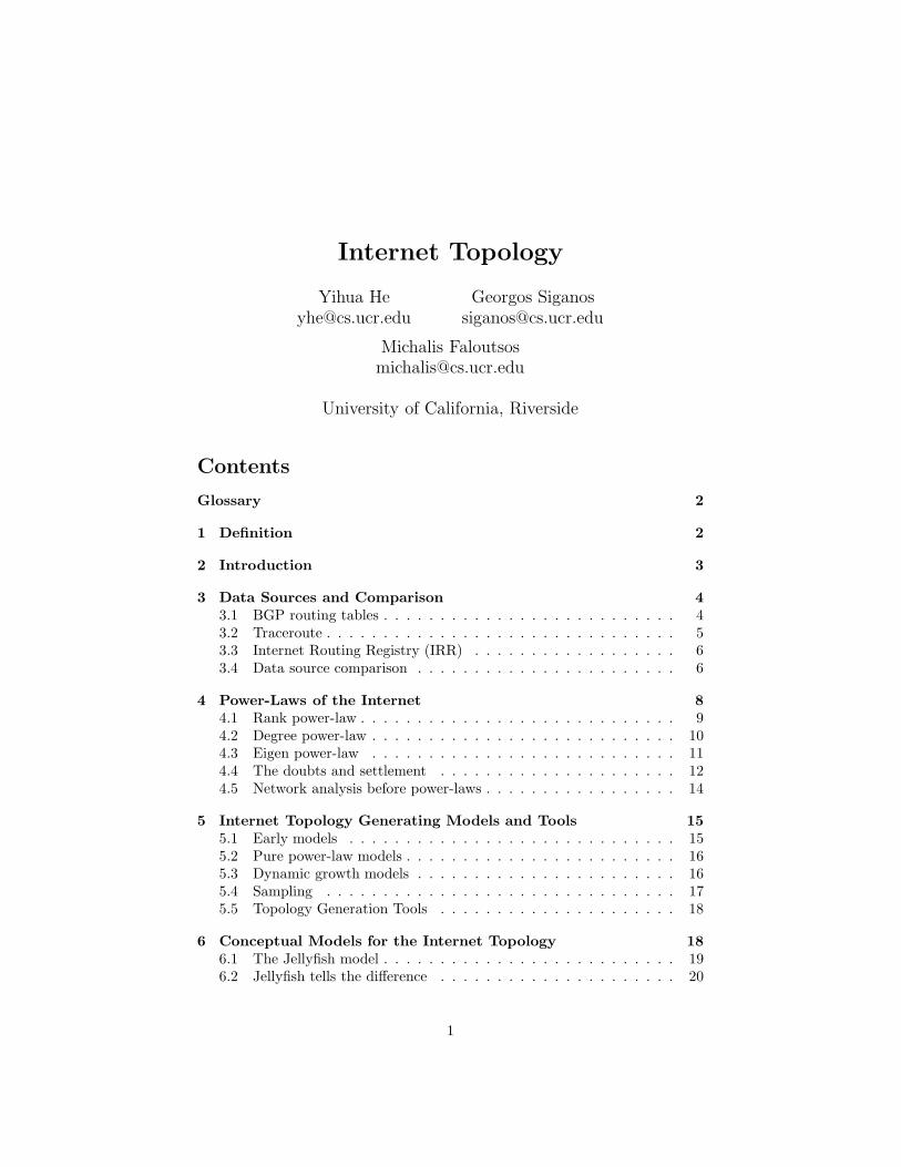
(a) Router level (b) AS level
Figure 1: The structure of Internet at two levels
information and they are harder to get. (3)AS-level topology is not directly en-gineered by human; instead, it is driven by technological and economical forces.
The research on Internet topology is driven by the explosive growth of theInternet, which has been accompanied by a wide range of inter-networking prob-lems related to routing, resource reservation and administration. The studyof algorithms and policies to address such problems often requires topologicalinformation and models. In 1999, Faloutsos brothers [1] discovered that theseemingly random Internet topology does follow some rules: it follows power-law distributions. This finding revolutionized the research on Internet topologyand generated much follow-up works.
2 Introduction
The Internet can be decomposed into connected subnetworks that are underseparate administrative authorities, as shown in Figure 1. These subnetworksare called domains or Autonomous Systems (ASes). The Internet communitydevelops and employs different routing protocols inside an AS and between ASes.An intra-domain protocol, such as RIP, IS-IS, or OSPF, is limited within an AS,while an inter-domain protocol, such as BGP, runs between ASes. This way, thetopology of the Internet can be studied at two different granularities. At therouter level, each router is represented by a node [2], and a direct connection(either inter-domain or intra-domain) between any pair of routers is representedby an edge. At the AS level, each AS is represented by a single node [3] andeach edge is an inter-domain interconnection. The study of the topology at bothlevels is equally important.
This article majorly focus on the AS level Internet topology. Note that,at this level, only one edge exists between two nodes, although there may bemultiple connections between two ASes in practice. This limitation is majorlydue to the nature of the data that the community has.
3
Network Next Hop (Other Fields) Path2.0.0.0/24 157.130.10.233 (...) 701 1299 34211 41856 41856
Table 1: An excerpt of an entry in typical Cisco “sh ip bgp” format BGP tabledumps from BGP collector “route-views.oregon-ix.net” on May 1, 2007.
There are multiple benefits from understanding the topology of the Internet.This is motivated by questions like the following “What does the Internet looklike?” “Are there any topological properties that don’t change in time?” “Howwill it look like a year from now?” “How can I generate Internet-like graphs formy simulations?”. Modeling the Internet topology is an important open prob-lem despite the attention it has attracted recently. Paxson and Floyd considerthis problem as a major reason why we don’t know how to simulate the Inter-net [4]. An accurate topological model can have signicant impact on networkresearch. First, we can design more efficient protocols that take advantage ofits topological properties. Second, we can create more accurate articial modelsfor simulation purposes. And third, we can derive estimates for topological pa-rameters that are useful for the analysis of protocols and for speculations of theInternet topology in the future.
In the rest of this article, we will first review how and where the Internettopology information is collected in Section 3. We also compare the pros andcons of different data sources and investigate the reason why they have suchdifference. In Section 4, we will review the power-laws of the Internet, whichis one of the most important discoveries of the Internet topology. The power-laws lead to significant follow-up works in modeling the Internet topology, andwe will discuss these models in Section 5 and Section 6. Then we exhibit thetechniques to discover the complete Internet topology in Section 7. At last, wediscuss future research directions of the Internet topology in Section 8.
3 Data Sources and Comparison
We first describe the data sources for collecting AS-level Internet topology. Allof these sources and methods have their shortcomings, which will be comparedat the end of this section.
3.1 BGP routing tables
BGP routing table dumps are probably the most widely used resource thatprovides information on the AS Internet topology. Normally, these routing tabledumps are obtained from special BGP collectors1, each of which connects withone or more Internet backbone routers in different ASes with special agreements.
1Normal BGP routing software runs on the BGP collectors. Therefore, each BGP collectorhas all functionalities of a normal BGP router; routing table dumps can be obtained fromthese BGP collectors.
4
These BGP collectors do not advertise any prefix (i.e., IP blocks) to the Internet,while they are configured to receive all routes that the Internet backbone routersadvertise to them. Therefore, these collectors are totally passive, and they haveno effect to the global Internet. Periodically, each collector dumps its full routingtables to Internet archives, which are available for download.
Table 1 shows an entry of typical Cisco “sh ip bgp” format BGP tabledumps from BGP collector “route-views.oregon-ix.net” on May 1, 2007. Thisentry indicates that, the destination network 2.0.0.0/24 can be reached via ASpath “701 1299 34211 41856”. Therefore, the instance of Internet topologyshould include four ASes (AS701, AS1299, AS34211 and AS41856) and threelinks (AS701-AS1299, AS1299-AS34211 and AS34211-AS41856). Typically aBGP collector’s routing table dump has more than a hundred thousands suchentries from each peer AS; the total number of entries often exceeds severalmillions. The number of ASes or routers that each BGP collector varies from afew to approximately one hundred. There are two well-maintained BGP routingtable collector agent: Oregon Routeviews[5] and RIPE RIS[6]. Each of theseagents maintains a number of BGP collectors over the world.
Besides routing tables, a BGP collector may also dump routing updatesreceived from its peers periodically. Routing updates have a similar format torouting tables. A BGP update message displays the current route to a prefix,and therefore, a collection of BGP updates is able to reveal the dynamic of BGProuting.
3.2 Traceroute
Traceroute[7] is a handy debugging program to discover the route that IP data-grams follow from one host to another. Traceroute takes advantage the factthat each router has to decrement the TTL (Time To Live) field by 1 for eachIP packet pass through it, and each router has to discard any IP packets withTTL=0 and send an ICMP “time-exceeded” error message back to the senderof the original IP packet. The original purpose of the action is to prevent IPpackets from circulating the network for ever. The operation of traceroute takeadvantage of this feature: it sends TTL increasing IP packets to the destination.These packets will expire at the routers along the path it reach the destination.Since each router along the path will send ICMP “time-exceeded” message backto the traceroute source, the identities of these routers (or more precisely, theoutgoing IP interfaces of those routers) can be discovered. Although there is noguarantees that two consecutive IP packets will traverse the same route to thesame destination, most often they do.
Skitter[8] is a part of CAIDA’s [9] topology measurement project. CAIDA[9] maintains a set of (about 20) active monitors distributed around the globe.Each monitor uses a modified version of traceroute to probe a large set of IPaddresses which nearly cover the whole IP address space. Rocketfuel [10] is atopology discovery project from University of Washington. Rocketfuel use alarger number (a few hundreds) of traceroute sources from public tracerouteservers as their sources. Therefore Rocketfuel has significant more number of
5
vantage points. However, due to restrictions of the public traceroute servers,the rate of traceroute probing is limited in Rocketfuel. Therefore Rocketfuel isbetter at probing specific ISP networks but not the whole Internet. Anotherpromising project is NetDimes [11] from Telaviv University. To increase thenumber of vantage points, NetDimes distribute a large number (tens of thou-sands) of probing agents to global Internet users on volunteer basis. Theseagents perform traceroutes according to the NetDimes center controls. Sincethe agents are most volunteers, coordination is still hard in order to probe theInternet topology from anywhere at any given time.
All traceroute probes only reflect router-level topology. In order to obtainAS level Internet topology, the probed IP addresses have to be mapped to theASes that they belong to. The conventional way to map an IP address to its ASnumber is by looking up the IP block in the BGP routing tables with the longestprefix match. For example, if there is an IP address 2.0.0.18 and the longestprefix that it matches in the routing table is 2.0.0.0/24 (as shown in Table 1),then the announcing AS, which is the AS appeared at the end of the “Path”field, (AS41856 in Table 1) is the AS that the IP 2.0.0.18 should be mapped to.However, the accuracy of such conversion may suffer in certain situations. Maoet. al. [12][13] discussed them in details.
3.3 Internet Routing Registry (IRR)
The need for cooperation between Autonomous Systems is fulfilled today bythe Internet Routing Registries (IRR) [6]. ASes use the Routing Policy Spec-ification Language (RPSL) [7] [8] to describe their routing policy, and routerconfiguration files can be produced from it. At present, there exist 55 registries,which form a global database to obtain a view of the global routing policy.Some of these registries are regional, like RIPE or APNIC, other registries de-scribe the policies of an Autonomous System and its customers, for example,cable and wireless CW or LEVEL3. The main uses of the IRR registries areto provide an easy way for consistent configuration of filters, and a mean tofacilitate the debugging of Internet routing problems. From the registered rout-ing export and import policies, Internet topology can be extracted from IRR.For example, in Table 2, an excerpt of aut-num record for AS3303 in IRR isshown. From the registered import and export policy in this excerpt, the Inter-net topology should include three ASes (AS3303, AS701 and AS1239), and twoedges (AS3303-AS701 and AS3303-AS1239).
3.4 Data source comparison
BGP table dumps, especially the one from Oregon Routeview project, are themost widely used source for Internet topology study. An advantage of the BGProuting tables is that their link information is considered reliable. If an ASlink appears in a BGP routing table dump, it is almost certain that the linkexists. However, limited number of vantage points makes it hard to discovera more complete view of the AS-level topology. A single BGP routing table
6
aut-num: AS3303as-name: SWISSCOMdescr: Swisscom Solutions Ltddescr: IP-Plus Internet Backbone... ...import: from AS701 action pref=700; accept ANYexport: to AS701 announce AS-SWCMGLOBALimport: from AS1239 action pref=700; accept ANYexport: to AS1239 announce AS-SWCMGLOBAL... ...
Table 2: An excerpt of IRR in plain text format for AS3303.
has the union of “shortest” or, more accurately, preferred paths with respect tothis point of observation. As a result, such a collection will not see edges thatare not on the preferred path for this point of observation. Several theoreticaland experimental efforts explore the limitations of such measurements [14][15].Worse, such incompleteness may be statistically biased based on the type of thelinks: peer-to-peer links are more likely to be missing from BGP routing tabledumps than provider-customer links, due to the selective exporting rules of BGP.Typically, a peer-to-peer link can only be seen in a BGP routing table of thesetwo peering ASes or their customers. Thus, given a peer-to-peer edge, unless aBGP collector peers with a customer of either AS incident to the edge, the edgecan not be detected from the table dumps of the BGP collector. A recent work[16] discusses in depth this limitation. Thus, apart from being incomplete, themeasured graph may not fairly represent the different types of links. Furthermore, BGP table dumps are likely to miss alternative and back-up paths. Bydefinition, a router advertises only the best path to each destination, namely anIP prefix. Therefore, the back-up paths will not show up in distant ASes unlessthe primary link breaks. To address the problem, a recent effort suggests theneed for actively probing backup links [17].
BGP updates are used in previous studies[18][19] as a source of topologicalinformation and they show that by collecting BGP updates over a period oftime, more AS links are visible. This is because as the topology changes, BGPupdates provide transient and ephemeral route information. However, if thewindow of observation is long, an advertised link may cease to exist [18] by thetime that we construct a topology snapshot. In other words, BGP updates mayprovide a superimposition of a number of different snapshots that existed atsome point in time. Note that BGP updates are collected at the same vantagepoints as the BGP tables in most collection sites. Naturally, topologies derivedfrom BGP updates share the same statistical bias per link type as from BGProuting tables: peer-to-peer links are only to be advertised to the peering ASesand their customers. This further limits the additional information that BGPupdates can provide currently. On the other hand, BGP updates could be useful
7
in revealing ephemeral backup links over long period of observation, along witherroneous BGP updates, which are not visible in the Internet at large, unlessthe primary link breaks down. To tell the two apart, we need highly targetedprobes. Recently, active BGP probing[17] has been proposed for identifyingbackup AS links. This is a promising approach that could complement ourwork and provide the needed capability for discovering more AS links.
By using traceroute, one can explore IP paths and then translate the IPaddresses to AS numbers, thus obtaining AS paths. Similar to BGP tables, thetraceroute path information is considered reliable, since it represents the path2
that the packets actually traverse. On the other hand, a traceroute serverexplores the routing paths from its location towards the rest of the world, andthus, the collected data has the same limitations as BGP data in terms ofcompleteness and link bias. One additional challenge with the traceroute datais the mapping of an IP path to an AS path. The problem is far from trivial,and it has been the focus of several recent efforts [12][13].
Internet Routing Registry (IRR)[20] is the union of a growing number ofworld-wide routing policy databases that use the Routing Policy SpecificationLanguage (RPSL). In principle, each AS should register routes to all its neigh-bors (that reflect the AS links between the AS and its neighbors) with thisregistry. IRR information is manually maintained and there is no stringent re-quirement for updating it. Therefore, without any processing, AS links derivedfrom IRR are prone to human errors, could be outdated or incomplete. How-ever, the up-to-date IRR entries provide a wealth of information that could notbe obtained from any other source. A recent effort [21] shows that, with carefulprocessing of the data, we can extract a non-trivial amount of correct and usefulinformation.
4 Power-Laws of the Internet
The power-laws for Internet topology are first observed by Faloutsos brothers [1],and later summarized in [22]. In those two papers, the authors have shown thatthe Internet topology at the AS level can be described efficiently with power-laws. The elegance and simplicity of the power-laws provide a novel perspectiveinto the seemingly uncontrolled Internet structure.
Power-laws are expressions of the form y ∝ xa, where a is a constant, x andy are the measures of interest, and ∝ stands for “proportional to”. Pareto wasamong the first to introduce power-laws in 1896 [23]. He used power-laws to de-scribe the distribution of income where there are few very rich people, but mostof the people have a low income. Another classical law, the Zipf law [24], wasintroduced in 1949, for the frequencies of the English words and the populationof cities. More recently, power-laws have been observed in communication net-works. First, power-laws have been observed in traffic [25][26][27]. In addition,the topology of the World Wide Web [28, 29] can be described by power-laws.
2An exception is when the route changes while a path is being explored by a traceroute.
8
1
10
100
1000
10000
1 10 100 1000 10000 100000
’P1.Oregon’exp(6.8968) *x**(-0.7444)
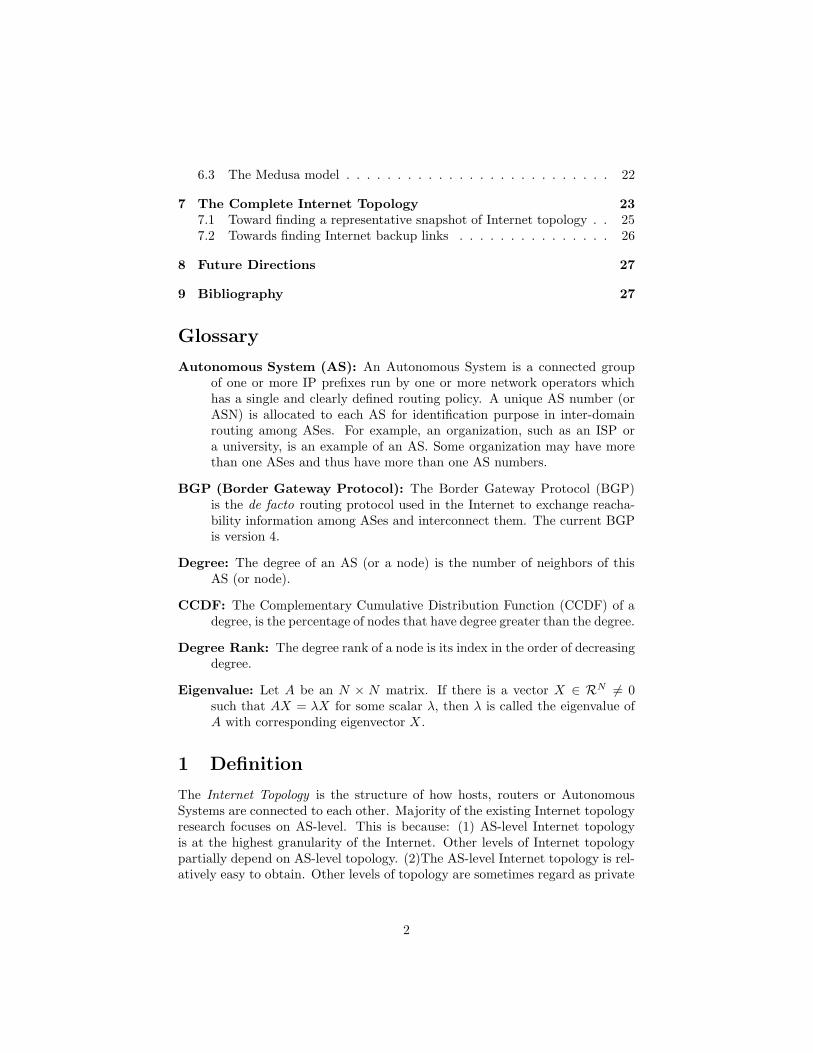
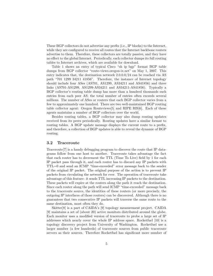
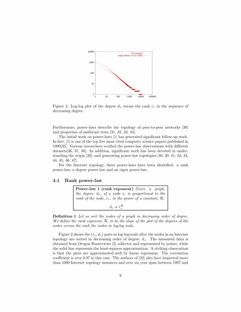
Figure 2: Log-log plot of the degree dv versus the rank rv in the sequence ofdecreasing degree.
Furthermore, power-laws describe the topology of peer-to-peer networks [30]and properties of multicast trees [31, 32, 33, 34].
The initial work on power-laws [1] has generated significant follow-up work.In fact, [1] is one of the top five most cited computer science papers published in1999[35]. Various researchers verified the power-law observations with differentdatasets[36, 37, 38]. In addition, significant work has been devoted in under-standing the origin [39], and generating power-law topologies [40, 39, 41, 42, 43,44, 45, 46, 47].
For the Internet topology, three power-laws have been identified: a rankpower-law, a degree power-law and an eigen power-law.
4.1 Rank power-law
Power-law 1 (rank exponent) Given a graph,the degree, dv, of a node v, is proportional to therank of the node, rv, to the power of a constant, R:
dv ∝ rRv
Definition 1 Let us sort the nodes of a graph in decreasing order of degree.We define the rank exponent, R, to be the slope of the plot of the degrees of thenodes versus the rank the nodes in log-log scale.
Figure 2 shows the (rv , dv) pairs in log-log scale after the nodes in an Internettopology are sorted in decreasing order of degree, dv . The measured data isobtained from Oregon Routeviews [5] collector and represented by points, whilethe solid line represents the least-squares approximation. A striking observationis that the plots are approximated well by linear regression. The correlationcoefficient is over 0.97 in this case. The authors of [22] also have inspected morethan 1000 Internet topology instances and over six year span between 1997 and
9
1e-05
0.0001
0.001
0.01
0.1
1
1 10 100 1000 10000
’P2.Oregon’exp(-0.4732) *x**(-1.1265)
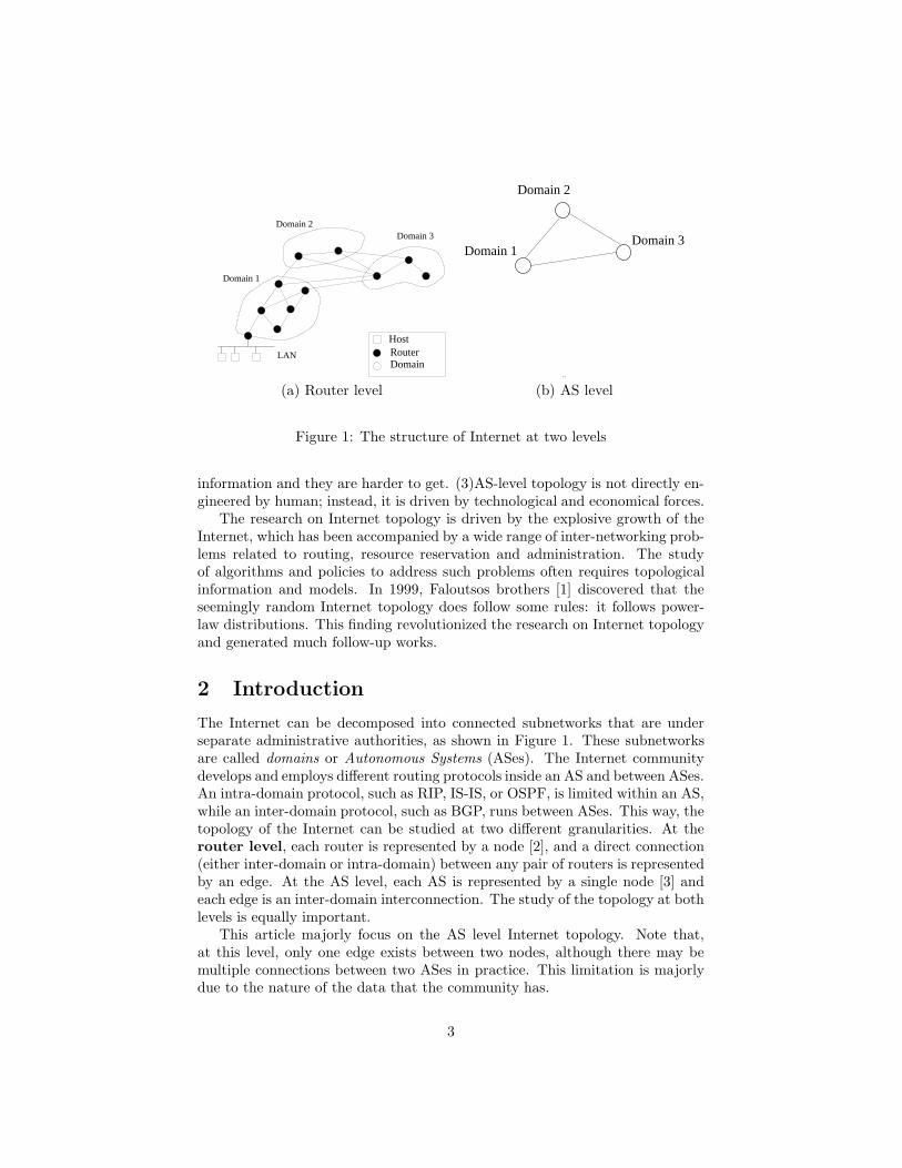
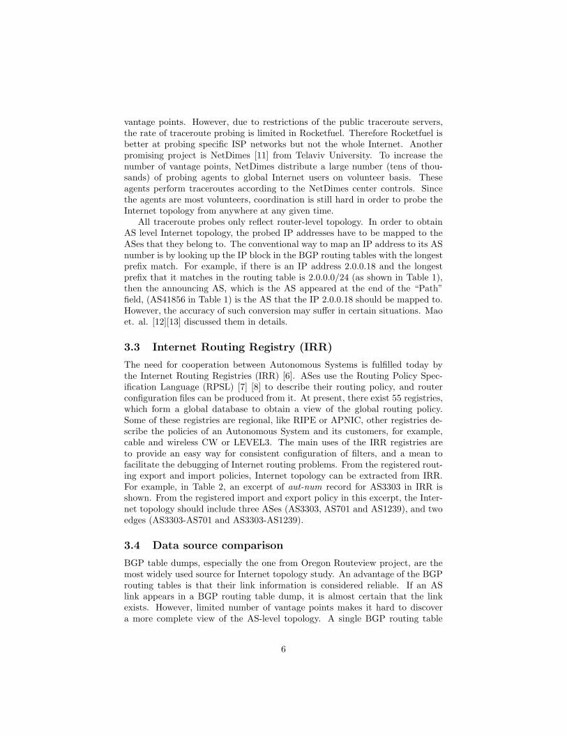
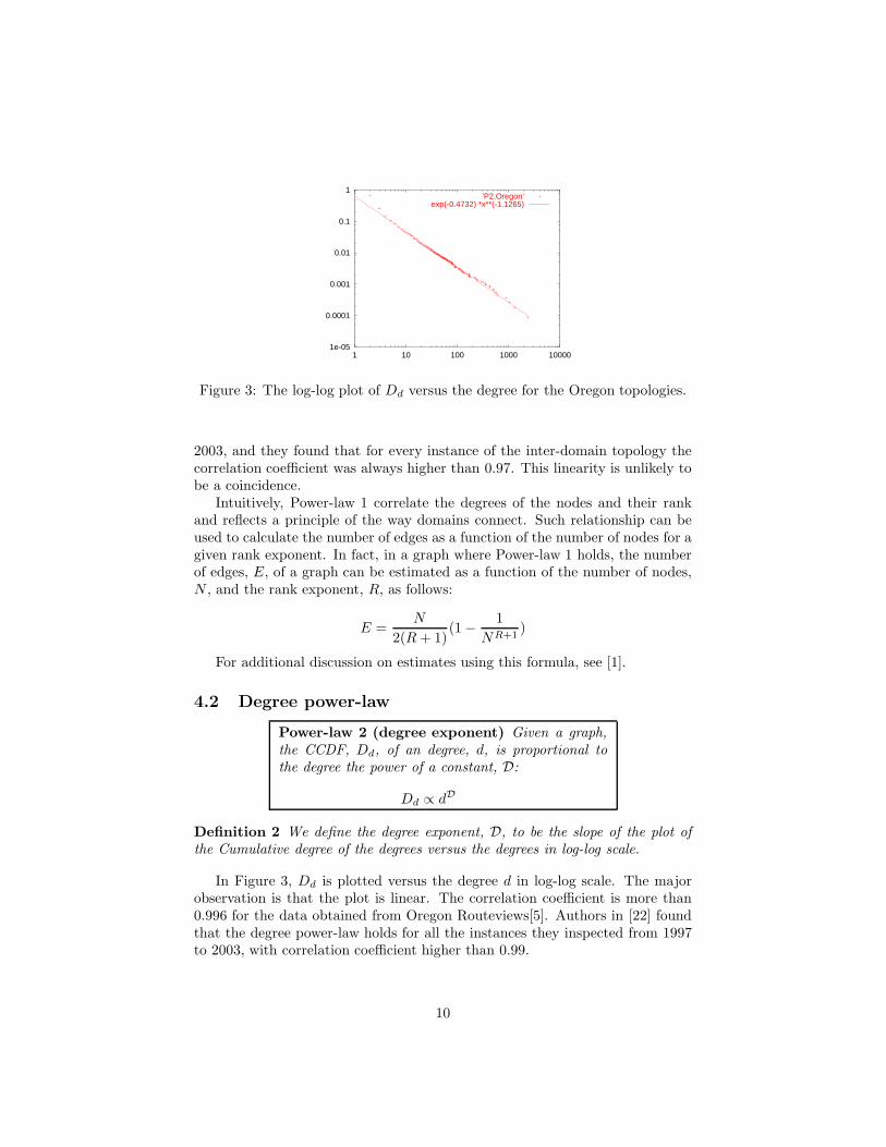
Figure 3: The log-log plot of Dd versus the degree for the Oregon topologies.
2003, and they found that for every instance of the inter-domain topology thecorrelation coefficient was always higher than 0.97. This linearity is unlikely tobe a coincidence.
Intuitively, Power-law 1 correlate the degrees of the nodes and their rankand reflects a principle of the way domains connect. Such relationship can beused to calculate the number of edges as a function of the number of nodes for agiven rank exponent. In fact, in a graph where Power-law 1 holds, the numberof edges, E, of a graph can be estimated as a function of the number of nodes,N , and the rank exponent, R, as follows:
E =N
2(R + 1)(1 −
1
NR+1)
For additional discussion on estimates using this formula, see [1].
4.2 Degree power-law
Power-law 2 (degree exponent) Given a graph,the CCDF, Dd, of an degree, d, is proportional tothe degree the power of a constant, D:
Dd ∝ dD
Definition 2 We define the degree exponent, D, to be the slope of the plot ofthe Cumulative degree of the degrees versus the degrees in log-log scale.
In Figure 3, Dd is plotted versus the degree d in log-log scale. The majorobservation is that the plot is linear. The correlation coefficient is more than0.996 for the data obtained from Oregon Routeviews[5]. Authors in [22] foundthat the degree power-law holds for all the instances they inspected from 1997to 2003, with correlation coefficient higher than 0.99.
10
1
10
100
1 10 100
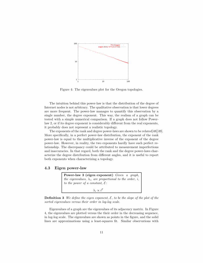
’P3.Oregon’exp(4.3031) *x**(-0.47734)
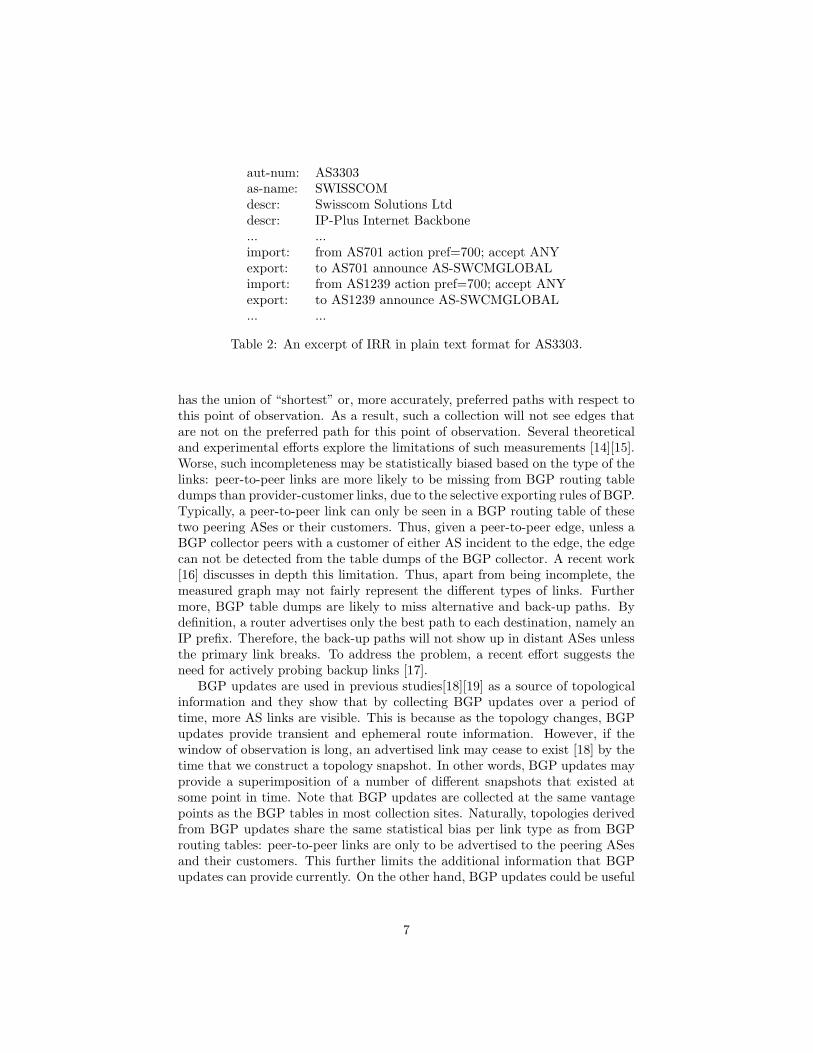
Figure 4: The eigenvalues plot for the Oregon topologies.
The intuition behind this power-law is that the distribution of the degree ofInternet nodes is not arbitrary. The qualitative observation is that lower degreesare more frequent. The power-law manages to quantify this observation by asingle number, the degree exponent. This way, the realism of a graph can betested with a simple numerical comparison. If a graph does not follow Power-law 2, or if its degree exponent is considerably different from the real exponents,it probably does not represent a realistic topology.
The exponents of the rank and degree power-laws are shown to be related[48][49].More specifically, in a perfect power-law distribution, the exponent of the rankpower-law is equal to the multiplicative inverse of the exponent of the degreepower-law. However, in reality, the two exponents hardly have such perfect re-lationship. The discrepancy could be attributed to measurement imperfectionsand inaccuracies. In that regard, both the rank and the degree power-laws char-acterize the degree distribution from different angles, and it is useful to reportboth exponents when characterizing a topology.
4.3 Eigen power-law
Power-law 3 (eigen exponent) Given a graph,the eigenvalues, λi, are proportional to the order, i,to the power of a constant, E:
λi ∝ iE
Definition 3 We define the eigen exponent, E, to be the slope of the plot of thesorted eigenvalues versus their order in log-log scale.
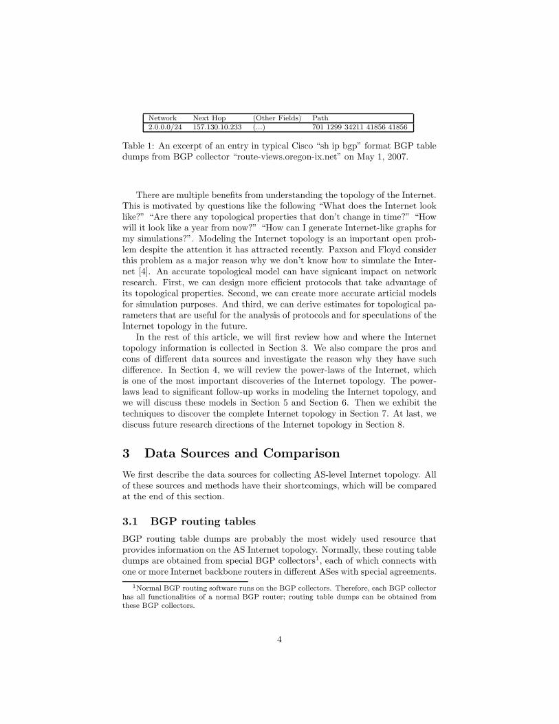
Eigenvalues of a graph are the eigenvalues of its adjacency matrix. In Figure4, the eigenvalues are plotted versus the their order in the decreasing sequence,in log-log scale. The eigenvalues are shown as points in the figure, and the solidlines are approximations using a least-squares fit. Similar observations with
11
equally high correlation coefficients were observed for all instances obtainedbetween 1997 and 2003 [22]. The plot is practically linear with a correlationcoefficient of 0.996, which constitutes an empirical power-law of the Internettopology.
Eigenvalues are fundamental graph metrics. There is a rich literature thatproves that the eigenvalues of a graph are closely related to many basic topo-logical properties such as the diameter, the number of edges, the number ofspanning trees, the number of connected components, and the number of walksof a certain length between vertices, as shown in [50]. Interestingly, Mihail etal. [51] show that there is a surprising relationship between the eigen expo-nent and the degree exponent: the eigen exponent is approximately the halfof the degree exponent. In practice, the exponents obey adequately the math-ematical relationship, although the match is naturally not perfect. All of theabove suggest that the eigenvalues intimately relate to topological properties ofgraphs. However, it is not trivial to explore the nature and the implications ofthis power-law.
4.4 The doubts and settlement
There has been doubts and debate on whether the degree distribution of theInternet at the AS level follows a exact power-law [46][52]. The major concernis that by adding new edges discovered from a number of sources other thanthe most used Oregon Routeviews [5], the degree distribution of the Internettopology deviates from a perfect power-law.
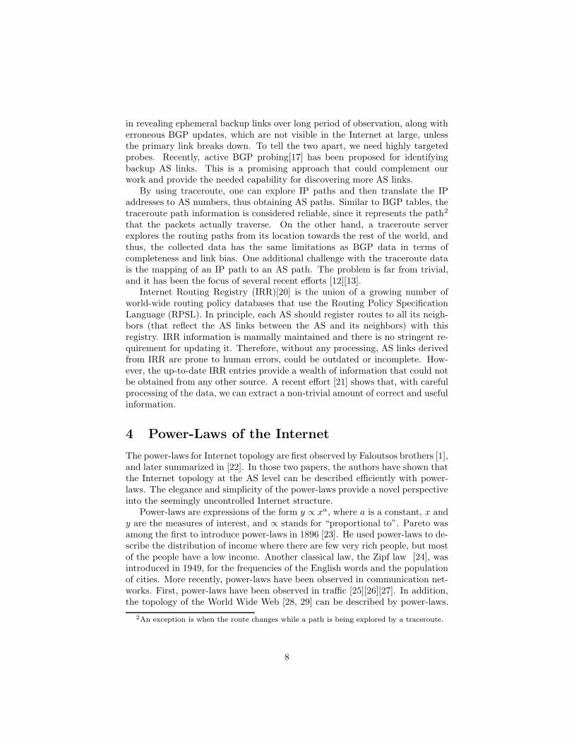
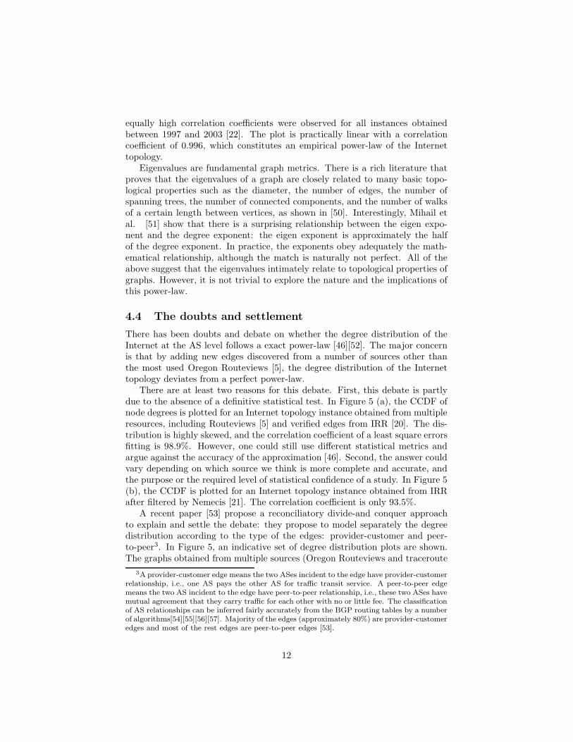
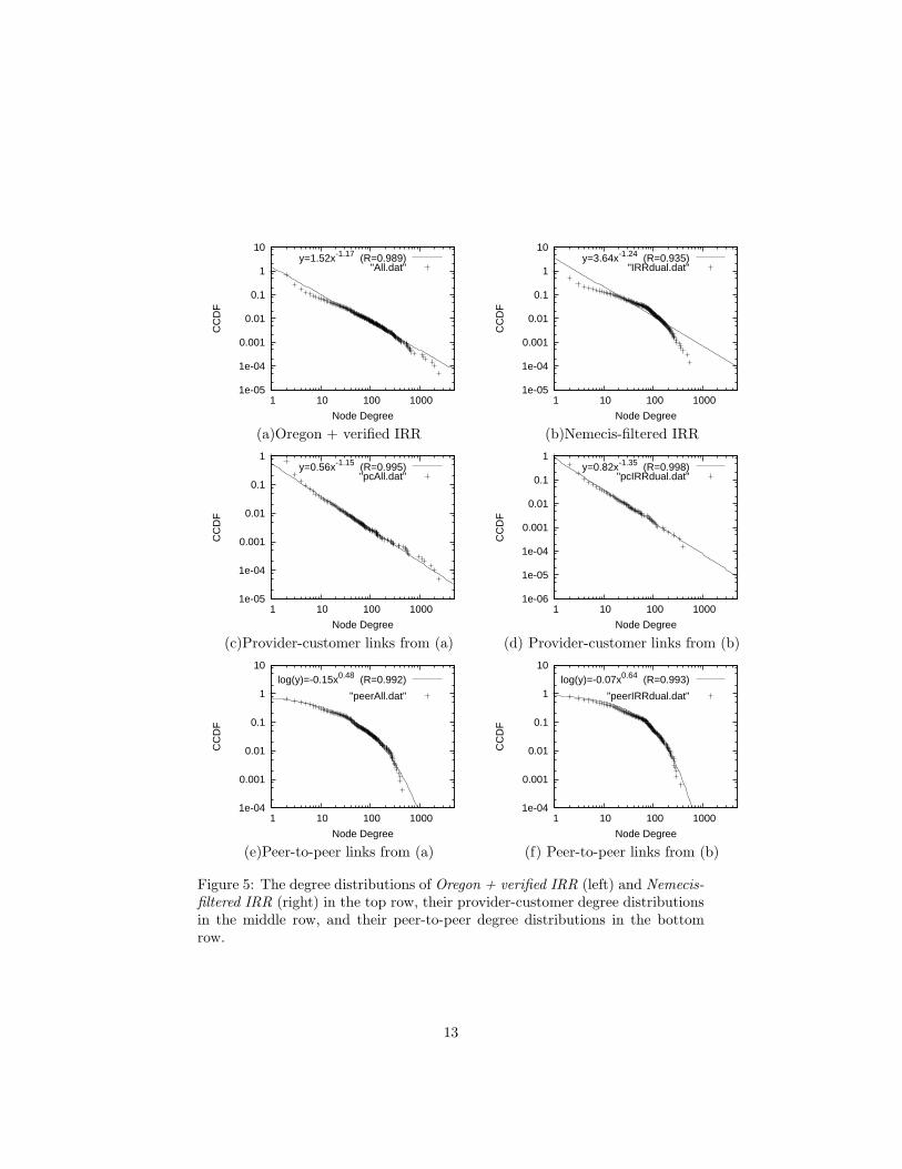
There are at least two reasons for this debate. First, this debate is partlydue to the absence of a definitive statistical test. In Figure 5 (a), the CCDF ofnode degrees is plotted for an Internet topology instance obtained from multipleresources, including Routeviews [5] and verified edges from IRR [20]. The dis-tribution is highly skewed, and the correlation coefficient of a least square errorsfitting is 98.9%. However, one could still use different statistical metrics andargue against the accuracy of the approximation [46]. Second, the answer couldvary depending on which source we think is more complete and accurate, andthe purpose or the required level of statistical confidence of a study. In Figure 5(b), the CCDF is plotted for an Internet topology instance obtained from IRRafter filtered by Nemecis [21]. The correlation coefficient is only 93.5%.
A recent paper [53] propose a reconciliatory divide-and conquer approachto explain and settle the debate: they propose to model separately the degreedistribution according to the type of the edges: provider-customer and peer-to-peer3. In Figure 5, an indicative set of degree distribution plots are shown.The graphs obtained from multiple sources (Oregon Routeviews and traceroute
3A provider-customer edge means the two ASes incident to the edge have provider-customerrelationship, i.e., one AS pays the other AS for traffic transit service. A peer-to-peer edgemeans the two AS incident to the edge have peer-to-peer relationship, i.e., these two ASes havemutual agreement that they carry traffic for each other with no or little fee. The classificationof AS relationships can be inferred fairly accurately from the BGP routing tables by a numberof algorithms[54][55][56][57]. Majority of the edges (approximately 80%) are provider-customeredges and most of the rest edges are peer-to-peer edges [53].
12
1e-05
1e-04
0.001
0.01
0.1
1
10
1 10 100 1000
CC
DF
Node Degree
y=1.52x-1.17 (R=0.989)"All.dat"
1e-05
1e-04
0.001
0.01
0.1
1
10
1 10 100 1000
CC
DF
Node Degree
y=3.64x-1.24 (R=0.935)"IRRdual.dat"
(a)Oregon + verified IRR (b)Nemecis-filtered IRR
1e-05
1e-04
0.001
0.01
0.1
1
1 10 100 1000
CC
DF
Node Degree
y=0.56x-1.15 (R=0.995)"pcAll.dat"
1e-06
1e-05
1e-04
0.001
0.01
0.1
1
1 10 100 1000
CC
DF
Node Degree
y=0.82x-1.35 (R=0.998)"pcIRRdual.dat"
(c)Provider-customer links from (a) (d) Provider-customer links from (b)
1e-04
0.001
0.01
0.1
1
10
1 10 100 1000
CC
DF
Node Degree
log(y)=-0.15x0.48 (R=0.992)
"peerAll.dat"
1e-04
0.001
0.01
0.1
1
10
1 10 100 1000
CC
DF
Node Degree
log(y)=-0.07x0.64 (R=0.993)
"peerIRRdual.dat"
(e)Peer-to-peer links from (a) (f) Peer-to-peer links from (b)
Figure 5: The degree distributions of Oregon + verified IRR (left) and Nemecis-filtered IRR (right) in the top row, their provider-customer degree distributionsin the middle row, and their peer-to-peer degree distributions in the bottomrow.
13
verified IRR links) are plotted in the left column ((a), (c), and (e)), and thetopology obtained from Nemecis-filtered IRR are plotted in the right column((b), (d), and (f)). The distributions for the whole graph are shown in the toprow, the provide-customer edges only in the middle row, and the peer-to-peeredges only in the bottom row. The power-law approximation in the first tworows of plots and the Weibull approximation in the bottom row of plots areshown.
The following two properties can be observed from Figure 5: (1)The provider-customer-only degree distribution can be accurately approximated by a power-law. The correlation coefficient is 99.5% or higher in the plots of Figure 5 (d)and (e). Note that, although the combined degree distribution of the topology inIRR does not follow a power law as shown in Figure 5 (b), its provider-customersubgraph follows a strict power law in Figure 5 (d). (2)The peer-to-peer-onlydegree distribution can be accurately approximated by a Weibull distribution.The correlation coefficient is 99.2% or higher in the plots of Figure 5 (e) and (f).It is natural to ask why the two distributions differ. The following could be oneof the explanations. Power-laws are related to the rich-get-richer behavior: lowdegree nodes “want” to connect to high degree nodes. For provider-customeredges, this makes sense: an AS wants to connect to a high-degree provider,since that provider would likely provide shorter paths to other ASes. Thisis less obviously true for peer-to-peer edges. If AS1 becomes a peer of AS2,AS1 does not benefit from the other peer-to-peer edges of AS2 due to routingpolicies[58]: an AS normally will not carry traffic from one of its peers to itsother peers. Therefore, high peer-to-peer degree does not make a node moreattractive as a peer-to-peer neighbor. The validity of this explanation is stillunder investigation[53].
4.5 Network analysis before power-laws
Before the discovery of power-law distribution of Internet topology, the metricsthat had been used to describe graphs were mainly the node degree and thedistances between nodes. Given a graph, the distance between two nodes isthe number of edges along the shortest path between the two nodes. Moststudies report minimum, maximum, and average values and plot the degree anddistance distribution. Govindan and Reddy [3] study the growth of the inter-domain topology of the Internet between 1994 and 1995. The graph is sparsewith 75% of the nodes having degrees less or equal to two. Pansiot and Grad[2] study the topology of the Internet in 1995 at the router level. The distancesthey report are approximately two times larger compared to those of Govindanand Reddy.
For graph generation purposes, Waxman introduced what seemed to be oneof the most popular network models [59]. These graphs are created probabilisti-cally considering the distance between nodes in a Euclidean sense. This modelwas successful in representing small early networks such as the ARPANET.As the size and the complexity of the network increased more detailed modelswere needed [60] [61]. Zegura et al. [61] introduce a comprehensive model that
14
includes several previous models.
5 Internet Topology Generating Models and Tools
An abstraction or model of the actual Internet topology is important to theunderstanding of how the topology is formed and how Internet topology is goingto be like in the future. Generated topologies are useful in assessing proposedsolutions (such as routing protocols) and provide rigous foundations of analysesof how the results scale or how they might change with a different topology.
5.1 Early models
The most simple model is probably the Pure Random model. In this model,a set of nodes is distributed in a plane, and an edge is added between eachpair of the nodes with a fixed probability p. Although this model does notexplicitly attempt to reflect any structure of real networks, it is attractive forits simplicity.
The Waxman [59] model, on the other hand, adds edges with a probabilitythat is some function of the distance between the node. This probability for anedge between node u and node v is given by:
P (u, v) = αe−d/(βL) (1)
where 0 < α, β ≤ 1, d is the Euclidean distance from u to v, and L is themaximum distance between any two nodes. There are several variations in ofthe Waxman model[62][63][61].
The Transit-Stub [64] method tries to impose a more Internet-orientedhierarchical structure as follows. A connected random graph is first generated(e.g. using the Waxman method described above). Each node in that graphrepresents an entire Transit domain. Each Transit domain node is expandedto form another connected random graph, representing the backbone topologyof that transit domain. Next, for each node in each transit domain, a numberof connected random graphs are generated, representing Stub domains that areattached to that transit node. Finally, some extra connectivity is added, in theform of “back-door” links between pairs of nodes, where a pair consists of a nodefrom a transit domain and another from a stub domain, or one node from eachof two different stub domains. By having nodes of different types, it is possibleto generate large sparsely-connected Internet-like topologies with typically lownode degrees. GT-ITM(Georgia Tech Internetwork Topology Models) is a toolto generate the Transit-Stub networks.
The problem of these early models is that they do not follow power-laws asshown in the real Internet instances. Medina et. al. [40] tested the generatedtopologies from Waxman and Transit-Stub, and they found both of them exhibitthe absence or weak presence of the power-law.
15
5.2 Pure power-law models
Since the discovery of power-laws by Faloutsos brothers[1], the main focus of gen-erating an Internet-like topology has shifted to matching the exhibited power-law in the Internet.
Palmer et. al. [65] proposed the PLOD (Power Law Out-Degree) model. Inthis model, a degree credit is first assigned to each node in a graph with a givennumber of nodes. The degree distribution complies with the appropriate power-laws. Then an edge placement loop is executed: it randomly picks two nodesand assigns an edge if they are not connected and each node still has remainingdegree credit. After an edge is assigned, the degree credit of the nodes incidentto the edge will be deducted accordingly. The loop continues until there are nomore pairs of nodes that fulfill the condition.
The concept of PLRG (Power Law Random Graph) [66] was proposed byAiello et al. in the year 2000, and therefore this model is also sometimes calledModel A. In this model, a random graph is produced with power law degreedistribution depending on two parameters, which roughly delineate the size anddensity but they are natural and convenient for describing a power law degreesequence. The power law random graph model P (α, β) is described as follows.Let y be the number of nodes with degree x. P (α, β) assigns uniform probabilityto all graphs with y = eα/xβ , where α is the intercept and β is the (negative)slope when the degree sequence is plotted on a log-log scale. After the degreedistribution is defined, a set, L, which contains deg(v) distinct copies of eachnode v, will be formed. Then a random matching of the elements of L is chosen.For two nodes u and v, the number of edges joining u and v is equal to thenumber of edges in the matching of L joining copies of u to copies of v. Thegraph formed in the end is the PLRG.
These power-law “matchers” do not attempt to answer how a graph comesto have a power law degree sequence. Rather, they take that as a given. Surpris-ingly, these method seem to be able to match many other topology properties[67] of the real Internet.
5.3 Dynamic growth models
In contrast to the pure power-law model, the dynamic growth models try togenerate the Internet topology graph by simulating the growth of the Internet.
Barabasi and Albert [68] proposed a generic model (or BA Model) fornetwork growth:
1. Incremental growth: The network expands continuously by the addi-tion of new nodes.
2. Preferential attachment: A new node attaches preferentially to nodesthat are already well connected.
In more detail, the network begins with a small number (m0) of connectednodes. New nodes are added to the network one at a time. The probabilityp(v) that a new node is connected to an existing node v is determined as thefollowing:
16
p(v) = dv/∑
j
dj (2)
where dv is the degree of node v and∑
j dj is the sum of degrees of allexisting nodes. In BA model, heavily linked nodes tend to quickly accumulateeven more links, while nodes with only a few links are unlikely to be chosen asthe destination for a new link. The new nodes have a “preference” to attachthemselves to the already heavily linked nodes. This is so called “rich-get-richer”phenomenon.
The AB model [69] extents the BA model by adding a third rewiring op-eration called “rewiring”. The rewiring operation consists of choosing m linksrandomly and re-wire each end of them according to the same preference ruleused in the BA model.
Bu et. al. [43] found that the graphs generated by PLRG, BA and AB modelshave different characteristic values real Internet graph in terms of path lengthand clustering coefficient. They proposed GLP (Generalized Linear Preference)[43], in which the probability p is:
p(v) = (dv − β)/∑
j
(dj − β) (3)
where beta ∈ (−∞, 0) is a tunable parameter. The smaller the value of β is,the less preference gives to high degree nodes.
All these dynamic growth models produces graphs with power-law distri-bution. However, it is still hard for these models to capture every topologicalproperty of the Internet. Authors in [67] show that even GLP does not followsome hierarchical properties of the Internet.
5.4 Sampling
All aforementioned models attempt to grow a graph, an approach called “con-structive”. One weakness of these constructive methods lies in their dependenceon the principles of construction, and the choice of parameter values. Further-more, they often focus on matching a certain number of topology properties,while fail to match some other. To address these problems, Krishnamurthy et al.[70] took a “reductive” approach: instead of trying to construct a graph, theytry to “sample” real topologies to produce a smaller graph. The idea is thathopefully the original properties, either well-know or unnoticed, can be keptduring the process of reduction. In more detail, they propose several reductionmethods:
DRV (Deletion of Random Vertex): Remove a random vertex, each withthe same probability. DRE (Deletion of Random Edge): Remove a randomedge, each with the same probability. DRVE (Deletion of Random Vertex orEdge): Select a vertex uniformly at random, and then delete an edge chosenuniformly at random from the edges incident on this vertex. DHYB-w (Hybridof DRVE/DRE): In this method, DRVE is executed with probability w and
17
DRE is executed with probability 1 − w, where w ∈ [0, 1]. This method wasmotivated by the study showing that sometimes DRVE and DRE had oppositeperformances with respect to different metrics.
The topologies sampled by both DRV and DRE methods are mathematicallyproved to follow power-law degree distribution. By comparing experimentaldata, the authors in [70] concluded that DHYB-0.8 is the best reduction method,and it also compares favorably to graph generation methods proposed previouslyin the literature. These sampling methods are successful to reduce a topologydown to 30% of the original size. Beyond that the statistical confidence is foundlow.
5.5 Topology Generation Tools
BRITE (Boston university Representative Internet Topology gEnerator) [71]isa universal topology generator. It implements a single generation model that hasseveral degrees of freedom with respect to how the nodes are placed in the planeand the properties of the interconnection method to be used. With differenceparameter settings, BRITE can generate either Waxman model or BA mode.
Inet[72] is an AS level Internet topology generator. Inet aims at reproducingthe connectivity properties of Internet topologies as power-laws and with otherimprovements. It initially assigns node degrees from a power-law distributionand then proceed to interconnect them using different rules. The current ver-sion Inet-3.0 improves from their previous versions by creating topologies withmore accurate degree distributions and minimum vertex covers as compared toInternet topologies. Inet-3.0’s topologies still do not well represent the Internetin terms of maximum clique size and clustering coefficient. These related prob-lems stress a need for a better understanding of Internet connectivity and willbe addressed in the future work.
6 Conceptual Models for the Internet Topology
The Internet topology is large, complex and constantly changing. Even withthe introduction of power-laws, which appears as a necessary though not suffi-cient condition for a topology to be realistic, a conceptual model of the topol-ogy [22][2][38] is still hard to get. Although the Internet is widely believed to behierarchical by construction, it is too interconnected for an obvious hierarchy[45].Several efforts to visualize the router-level topology have been made [73][8], how-ever they can not be recreated manually and they do not provide a memorablemodel.
One goal here is to develop an effective conceptual model: a model thatcan be easily drawn by hand, while at the same time, it captures significantmacroscopic properties. The Jellyfish [67] and Medusa [74] models are twoconceptual models proposed for the inter-domain Internet topology.
18
InstanceInt-11-1997 Int-06-2000 Int-07-2003
Layer No Nodes % of Nodes Nodes % of Nodes Nodes % of Nodes
Core/Layer-0 8 0.23 14 0.176 13 0.08Layer-1 1354 44.90 3659 46.25 7330 46.27Layer-2 1202 39.866 3090 39.05 7116 45.51Layer-3 396 13.134 1052 13.29 1078 6.89Layer-4 43 1.425 86 10.87 96 0.61Layer-5 12 0.398 10 0.12 1 0.0063
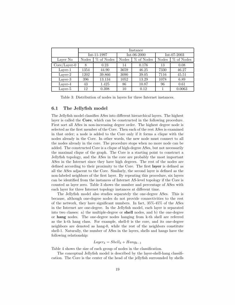
Table 3: Distribution of nodes in layers for three Internet instances.
6.1 The Jellyfish model
The Jellyfish model classifies ASes into different hierarchical layers. The highestlayer is called the Core, which can be constructed in the following procedure.First sort all ASes in non-increasing degree order. The highest degree node isselected as the first member of the Core. Then each of the rest ASes is examinedin that order; a node is added to the Core only if it forms a clique with thenodes already in the Core. In other words, the new node must connect to allthe nodes already in the core. The procedure stops when no more node can beadded. The constructed Core is a clique of high-degree ASes, but not necessarilythe maximal clique of the graph. The Core is a starting point to construct aJellyfish topology, and the ASes in the core are probably the most importantASes in the Internet since they have high degrees. The rest of the nodes aredefined according to their proximity to the Core. The first layer is defined asall the ASes adjacent to the Core. Similarly, the second layer is defined as thenon-labeled neighbors of the first layer. By repeating this procedure, six layerscan be identified from the instances of Internet AS-level topology if the Core iscounted as layer zero. Table 3 shows the number and percentage of ASes witheach layer for three Internet topology instances at different time.
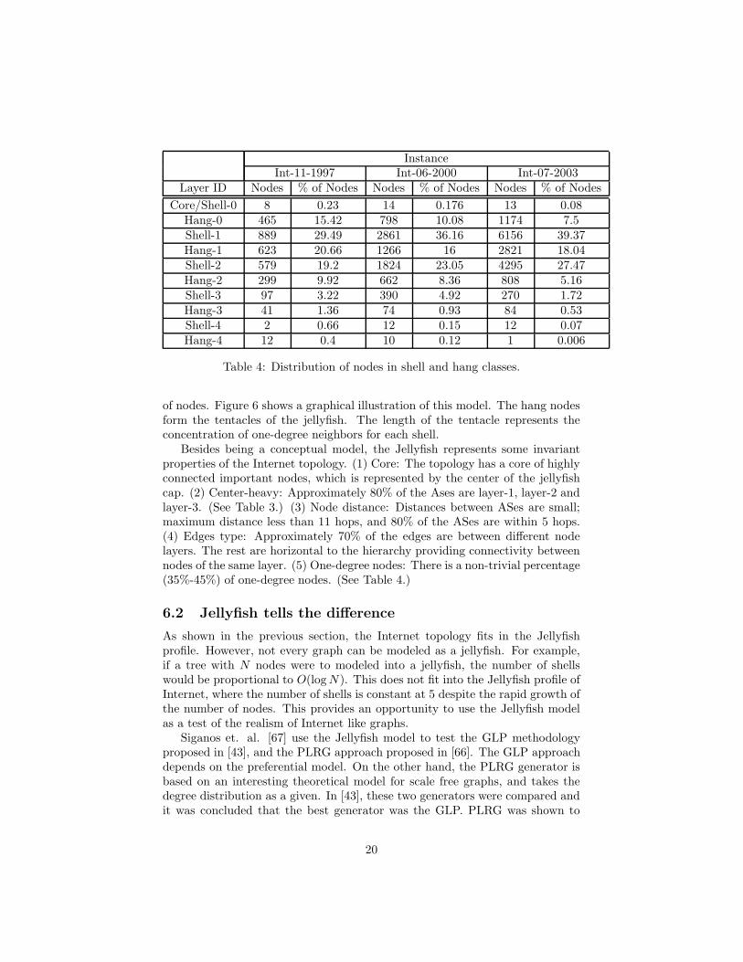
The Jellyfish model also studies separately the one-degree ASes. This isbecause, although one-degree nodes do not provide connectivities to the restof the network, they have significant numbers. In fact, 35%-45% of the ASesin the Internet are one-degree. In the Jellyfish model, each layer is separatedinto two classes: a) the multiple-degree or shell nodes, and b) the one-degreeor hang nodes. The one-degree nodes hanging from k-th shell are referredas the k-th hang class. For example, shell-0 is the core, and its one-degreeneighbors are denoted as hang-0, while the rest of the neighbors constituteshell-1. Naturally, the number of ASes in the layers, shells and hangs have thefollowing relationship:
Layerk = Shellk + Hangk−1
Table 4 shows the size of each group of nodes in the classification.The conceptual Jellyfish model is described by the layer-shell-hang classifi-
cation. The Core is the center of the head of the jellyfish surrounded by shells
19
InstanceInt-11-1997 Int-06-2000 Int-07-2003
Layer ID Nodes % of Nodes Nodes % of Nodes Nodes % of Nodes
Core/Shell-0 8 0.23 14 0.176 13 0.08Hang-0 465 15.42 798 10.08 1174 7.5Shell-1 889 29.49 2861 36.16 6156 39.37Hang-1 623 20.66 1266 16 2821 18.04Shell-2 579 19.2 1824 23.05 4295 27.47Hang-2 299 9.92 662 8.36 808 5.16Shell-3 97 3.22 390 4.92 270 1.72Hang-3 41 1.36 74 0.93 84 0.53Shell-4 2 0.66 12 0.15 12 0.07Hang-4 12 0.4 10 0.12 1 0.006
Table 4: Distribution of nodes in shell and hang classes.
of nodes. Figure 6 shows a graphical illustration of this model. The hang nodesform the tentacles of the jellyfish. The length of the tentacle represents theconcentration of one-degree neighbors for each shell.
Besides being a conceptual model, the Jellyfish represents some invariantproperties of the Internet topology. (1) Core: The topology has a core of highlyconnected important nodes, which is represented by the center of the jellyfishcap. (2) Center-heavy: Approximately 80% of the Ases are layer-1, layer-2 andlayer-3. (See Table 3.) (3) Node distance: Distances between ASes are small;maximum distance less than 11 hops, and 80% of the ASes are within 5 hops.(4) Edges type: Approximately 70% of the edges are between different nodelayers. The rest are horizontal to the hierarchy providing connectivity betweennodes of the same layer. (5) One-degree nodes: There is a non-trivial percentage(35%-45%) of one-degree nodes. (See Table 4.)
6.2 Jellyfish tells the difference
As shown in the previous section, the Internet topology fits in the Jellyfishprofile. However, not every graph can be modeled as a jellyfish. For example,if a tree with N nodes were to modeled into a jellyfish, the number of shellswould be proportional to O(log N). This does not fit into the Jellyfish profile ofInternet, where the number of shells is constant at 5 despite the rapid growth ofthe number of nodes. This provides an opportunity to use the Jellyfish modelas a test of the realism of Internet like graphs.
Siganos et. al. [67] use the Jellyfish model to test the GLP methodologyproposed in [43], and the PLRG approach proposed in [66]. The GLP approachdepends on the preferential model. On the other hand, the PLRG generator isbased on an interesting theoretical model for scale free graphs, and takes thedegree distribution as a given. In [43], these two generators were compared andit was concluded that the best generator was the GLP. PLRG was shown to
20
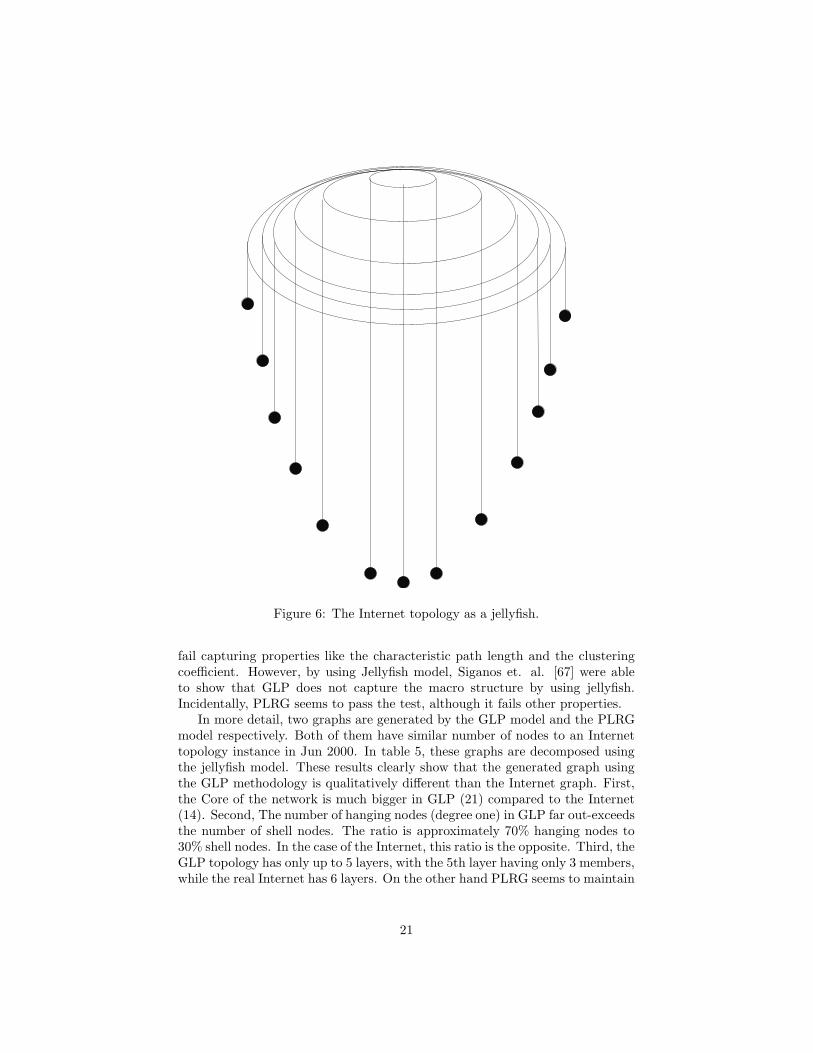
Figure 6: The Internet topology as a jellyfish.
fail capturing properties like the characteristic path length and the clusteringcoefficient. However, by using Jellyfish model, Siganos et. al. [67] were ableto show that GLP does not capture the macro structure by using jellyfish.Incidentally, PLRG seems to pass the test, although it fails other properties.
In more detail, two graphs are generated by the GLP model and the PLRGmodel respectively. Both of them have similar number of nodes to an Internettopology instance in Jun 2000. In table 5, these graphs are decomposed usingthe jellyfish model. These results clearly show that the generated graph usingthe GLP methodology is qualitatively different than the Internet graph. First,the Core of the network is much bigger in GLP (21) compared to the Internet(14). Second, The number of hanging nodes (degree one) in GLP far out-exceedsthe number of shell nodes. The ratio is approximately 70% hanging nodes to30% shell nodes. In the case of the Internet, this ratio is the opposite. Third, theGLP topology has only up to 5 layers, with the 5th layer having only 3 members,while the real Internet has 6 layers. On the other hand PLRG seems to maintain
21
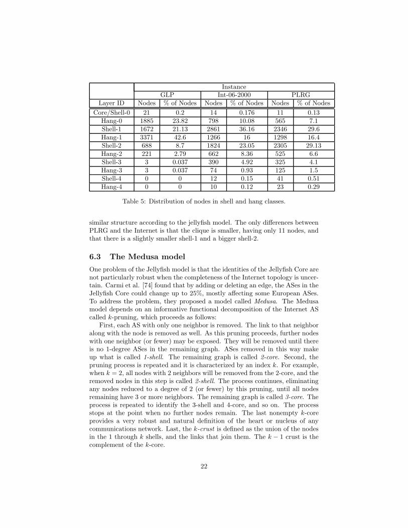
InstanceGLP Int-06-2000 PLRG
Layer ID Nodes % of Nodes Nodes % of Nodes Nodes % of Nodes
Core/Shell-0 21 0.2 14 0.176 11 0.13Hang-0 1885 23.82 798 10.08 565 7.1Shell-1 1672 21.13 2861 36.16 2346 29.6Hang-1 3371 42.6 1266 16 1298 16.4Shell-2 688 8.7 1824 23.05 2305 29.13Hang-2 221 2.79 662 8.36 525 6.6Shell-3 3 0.037 390 4.92 325 4.1Hang-3 3 0.037 74 0.93 125 1.5Shell-4 0 0 12 0.15 41 0.51Hang-4 0 0 10 0.12 23 0.29
Table 5: Distribution of nodes in shell and hang classes.
similar structure according to the jellyfish model. The only differences betweenPLRG and the Internet is that the clique is smaller, having only 11 nodes, andthat there is a slightly smaller shell-1 and a bigger shell-2.
6.3 The Medusa model
One problem of the Jellyfish model is that the identities of the Jellyfish Core arenot particularly robust when the completeness of the Internet topology is uncer-tain. Carmi et al. [74] found that by adding or deleting an edge, the ASes in theJellyfish Core could change up to 25%, mostly affecting some European ASes.To address the problem, they proposed a model called Medusa. The Medusamodel depends on an informative functional decomposition of the Internet AScalled k-pruning, which proceeds as follows:
First, each AS with only one neighbor is removed. The link to that neighboralong with the node is removed as well. As this pruning proceeds, further nodeswith one neighbor (or fewer) may be exposed. They will be removed until thereis no 1-degree ASes in the remaining graph. ASes removed in this way makeup what is called 1-shell. The remaining graph is called 2-core. Second, thepruning process is repeated and it is characterized by an index k. For example,when k = 2, all nodes with 2 neighbors will be removed from the 2-core, and theremoved nodes in this step is called 2-shell. The process continues, eliminatingany nodes reduced to a degree of 2 (or fewer) by this pruning, until all nodesremaining have 3 or more neighbors. The remaining graph is called 3-core. Theprocess is repeated to identify the 3-shell and 4-core, and so on. The processstops at the point when no further nodes remain. The last nonempty k-coreprovides a very robust and natural definition of the heart or nucleus of anycommunications network. Last, the k-crust is defined as the union of the nodesin the 1 through k shells, and the links that join them. The k − 1 crust is thecomplement of the k-core.
22
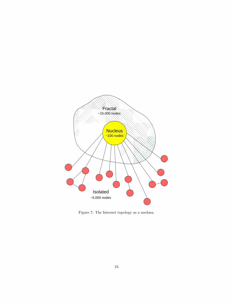
For small k, the crusts consist of many small clusters of connected sites.For sufficiently large k, the largest connected cluster of a k-crust consists of asignificant fraction of the whole k-crust, while no smaller cluster contains morethan a few nodes. The change occurs at a well-defined threshold value of k.There is a significant fraction of the nodes within each large-k crust which isnot part of its largest cluster, and remain isolated. Thus the AS graph (or anysimilar scale-free network) can be decomposed into three distinct components:
1. The nucleus (the innermost k-core)
2. The giant connected component of the last crust, in which only the nucleusis left out
3. The isolated components of the last crust, nodes forming many smallclusters. These connect to the connected component of the last crustonly through the nucleus
These three classes of nodes are quite different in their functional role withinthe Internet. The nucleus plays a critical role in BGP routing, since its nodes lieon a large fraction of the paths that connect different ASes. It allows redundancyin path construction, which gives immunity to multiple points of failure. Theconnected component of the large-k crusts could be an effective substrate onwhich to develop additional routing capacity, for messages that do not needto circle the globe. Finally, the isolated nodes and isolated groups of nodesin the last crust essentially leave all routing up to the nodes in the nucleus ofthe network. Because all their message traffic passes through the nucleus, evenwhen the destination is relatively close by, they may be contributing unnecessaryload to the most heavily used portions of the Internet. The relative size of thiscomponent could be a key indicator of the evolution of the topography of theInternet.
This model can be visualized as Figure 7. The core of the Medusa includesthe most important nodes that are found in the core and the first ring of theJellyfish’s mantle. The Jellyfish has relatively few rings around its core, whilethe Medusa’s mantle is more extended and differentiated. The tendrils hangingfrom the Jellyfish (leaf nodes) descend mostly from the core, but also fromall the other rings, while all the tendrils of the Medusa are, by construction,attached to its nucleus.
7 The Complete Internet Topology
An accurate topology model would be important for simulating, analyzing, anddesigning the future protocols effectively [4]. With an accurate Internet AS-leveltopology, first, one can design and analyze new inter-domain routing protocols,such as HLP [75], that take advantage of the properties of the Internet AS-level topology. Second, one can create more accurate models for simulationpurposes [76]. Third, one can analyze phenomena such as the spread of viruses
23
� � � � � � �� � � � � � �� � � � � � �� � � � � � �� � � � � � �� � � � � � �
� � �� � �� � �
Nucleus ~100 nodes
Isolated ~5,000 nodes
Fractal ~15,000 nodes
Figure 7: The Internet topology as a medusa.
24
[77][78], more accurately. In addition, the current initiatives of rethinking andredesigning the Internet and its operation from scratch would also benefit fromsuch an accurate Internet topology.
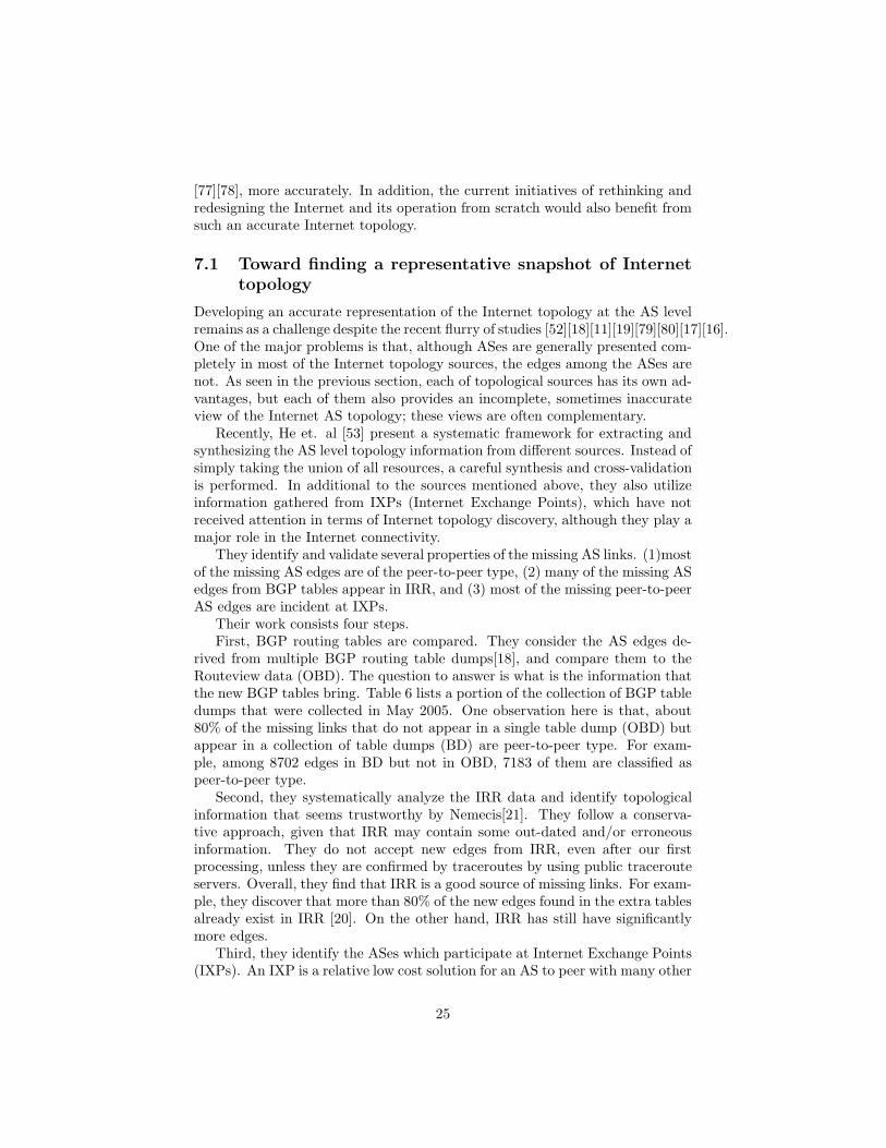
7.1 Toward finding a representative snapshot of Internettopology
Developing an accurate representation of the Internet topology at the AS levelremains as a challenge despite the recent flurry of studies [52][18][11][19][79][80][17][16].One of the major problems is that, although ASes are generally presented com-pletely in most of the Internet topology sources, the edges among the ASes arenot. As seen in the previous section, each of topological sources has its own ad-vantages, but each of them also provides an incomplete, sometimes inaccurateview of the Internet AS topology; these views are often complementary.
Recently, He et. al [53] present a systematic framework for extracting andsynthesizing the AS level topology information from different sources. Instead ofsimply taking the union of all resources, a careful synthesis and cross-validationis performed. In additional to the sources mentioned above, they also utilizeinformation gathered from IXPs (Internet Exchange Points), which have notreceived attention in terms of Internet topology discovery, although they play amajor role in the Internet connectivity.
They identify and validate several properties of the missing AS links. (1)mostof the missing AS edges are of the peer-to-peer type, (2) many of the missing ASedges from BGP tables appear in IRR, and (3) most of the missing peer-to-peerAS edges are incident at IXPs.
Their work consists four steps.First, BGP routing tables are compared. They consider the AS edges de-
rived from multiple BGP routing table dumps[18], and compare them to theRouteview data (OBD). The question to answer is what is the information thatthe new BGP tables bring. Table 6 lists a portion of the collection of BGP tabledumps that were collected in May 2005. One observation here is that, about80% of the missing links that do not appear in a single table dump (OBD) butappear in a collection of table dumps (BD) are peer-to-peer type. For exam-ple, among 8702 edges in BD but not in OBD, 7183 of them are classified aspeer-to-peer type.
Second, they systematically analyze the IRR data and identify topologicalinformation that seems trustworthy by Nemecis[21]. They follow a conserva-tive approach, given that IRR may contain some out-dated and/or erroneousinformation. They do not accept new edges from IRR, even after our firstprocessing, unless they are confirmed by traceroutes by using public tracerouteservers. Overall, they find that IRR is a good source of missing links. For exam-ple, they discover that more than 80% of the new edges found in the extra tablesalready exist in IRR [20]. On the other hand, IRR has still have significantlymore edges.
Third, they identify the ASes which participate at Internet Exchange Points(IXPs). An IXP is a relative low cost solution for an AS to peer with many other
25
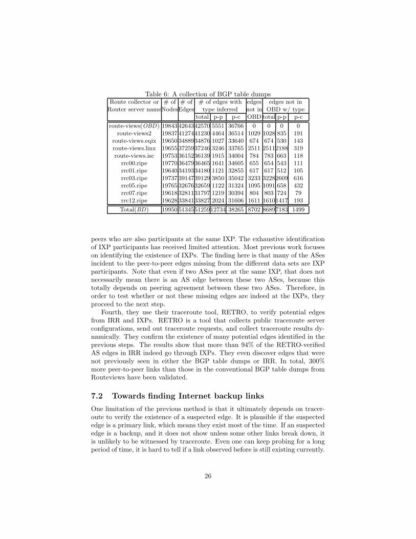
Table 6: A collection of BGP table dumpsRoute collector or # of # of # of edges with edges edges not in
Router server nameNodesEdges type inferred not in OBD w/ typetotal p-p p-c OBD total p-p p-c
route-views(OBD) 19843 4264342570 5551 36766 0 0 0 0route-views2 19837 4127441230 4464 36514 1029 1028 835 191
route-views.eqix 19650 3488934876 1027 33640 674 674 530 143route-views.linx 19655 3725937246 3246 33765 2511 25112188 319route-views.isc 19753 3615236139 1915 34004 784 783 663 118
rrc00.ripe 19770 3647936465 1641 34605 655 654 543 111rrc01.ripe 19640 3419334180 1121 32855 617 617 512 105rrc03.ripe 19737 3914739129 3850 35042 3233 32282609 616rrc05.ripe 19765 3267632659 1122 31324 1095 1091 658 432rrc07.ripe 19618 3281131797 1219 30394 804 803 724 79rrc12.ripe 19628 3384133827 2024 31606 1611 16101417 193
Total(BD) 19950 513455125912734 38265 8702 86897183 1499
peers who are also participants at the same IXP. The exhaustive identificationof IXP participants has received limited attention. Most previous work focuseson identifying the existence of IXPs. The finding here is that many of the ASesincident to the peer-to-peer edges missing from the different data sets are IXPparticipants. Note that even if two ASes peer at the same IXP, that does notnecessarily mean there is an AS edge between these two ASes, because thistotally depends on peering agreement between these two ASes. Therefore, inorder to test whether or not these missing edges are indeed at the IXPs, theyproceed to the next step.
Fourth, they use their traceroute tool, RETRO, to verify potential edgesfrom IRR and IXPs. RETRO is a tool that collects public traceroute serverconfigurations, send out traceroute requests, and collect traceroute results dy-namically. They confirm the existence of many potential edges identified in theprevious steps. The results show that more than 94% of the RETRO-verifiedAS edges in IRR indeed go through IXPs. They even discover edges that werenot previously seen in either the BGP table dumps or IRR. In total, 300%more peer-to-peer links than those in the conventional BGP table dumps fromRouteviews have been validated.
7.2 Towards finding Internet backup links
One limitation of the previous method is that it ultimately depends on tracer-oute to verify the existence of a suspected edge. It is plausible if the suspectededge is a primary link, which means they exist most of the time. If an suspectededge is a backup, and it does not show unless some other links break down, itis unlikely to be witnessed by traceroute. Even one can keep probing for a longperiod of time, it is hard to tell if a link observed before is still existing currently.
26
Recently, active BGP probing [17] has been proposed for identifying backupAS links. The main idea is to inject false AS path loops for an unused IP block.Since AS path loops are prohibited in inter-domain routing, BGP routers areforced to switch to backup links for this unused IP block. These links canbe observed from any route collectors, such as Routeviews or RIPE/RIS. Thisprobing technique does not affect normal Internet routing because every changeis restricted in the unused IP block.
In more detail, the principle of active BGP probing is the following. Anactive probing AS announces one of its prefixes with AS-paths including a num-ber of other ASes. These ASes, due to loop detection, will not use or propagatethe announcement. Then if there is any alternative path available, it will showup. To avoid influencing AS-path length, the prohibited ASes are placed in anAS-set at the end of the path. For example, to stop its announcement frombeing propagated by ASes 1, 2, and 3, an AS (say AS12654) might announceone of its prefixes with an AS-path of [12654 {1,2,3}]. This allows AS 12654 todiscover who propagates its announcements, find backup paths, and deduce thepolicies of other ASes with respect to its prefixes. By proper constructing the“prohibited” AS sets, one may be able to discover all backup links visible to theprobing AS.
Note, due to BGP export policies and very limited number of probingASes, this method majorly discovers provider-customer type backup links. Thismethod and the method of discovering missing peer-to-peer links [53] are com-plementary to each other.
8 Future Directions
degree-degree correlation sigcomm 2006, topology with directions (Gao) Topol-ogy generator and sampler for BGP simulation. Evolution (infocom 2006)Router-level topology discovery (NetDimes, iplane, rocketfuel)
9 Bibliography
Primary Literature(cited)
References
[1] M. Faloutsos, P. Faloutsos, and C. Faloutsos. On power-law relationshipsof the Internet topology. ACM SIGCOMM, pages 251–262, Sep 1-3, Cam-bridge MA, 1999.
[2] J.-J. Pansiot and D Grad. On routes and multicast trees in the Internet.ACM SIGCOMM Computer Communication Review, 28(1):41–50, January1998.
27
[3] R. Govindan and A. Reddy. An analysis of Internet Inter-domain topologyand route stability. Proc. IEEE INFOCOM, Kobe, Japan, April 7-11 1997.
[4] S. Floyd and V. Paxson. Difficulties in simulating the Internet. IEEETransaction on Networking, Aug 2001.
[5] Oregon routeview project, http://www.routeviews.org.
[6] Ripe route information service, http://www.ripe.net/ris.
[7] V. Jacobson. Traceroute. Internet Measurement Tool, 1995.
[8] Skitter, http://www.caida.org/tools/measurement/skitter/.
[9] The cooperative association for internet data analysis,http://www.caida.org.
[10] N. Spring, R. Mahajan, D. Wetherall, and T. Anderson. Measuring ISPtopologies with rocketfuel. IEEE/ACM Trans. Netw., 12(1):2–16, 2004.
[11] Y. Shavitt and E. Shir. DIMES: Let the Internet Measure Itself. ACMSIGCOMM Computer Communication Review (CCR), October 2005.
[12] Z. Mao, J. Rexford, J. Wang, and R. Katz. Towards an accurate AS-leveltraceroute tool. In Sigcomm, 2003.
[13] Z. Mao, D. Johnson, J. Rexford, J. Wang, and R. Katz. Scalable andaccurate identification of AS-Level forwarding paths. In Infocom, 2004.
[14] M. Crovella A. Lakhina, J. W. Byers and I. Matta. Sampling biases in iptopology measurements. In IEEE Infocom, 2003.
[15] D. Achlioptas, A. Clauset, D. Kempe, and C. Moore. On the bias of tracer-oute sampling, or power-law degree distributions in regular graphs. InSTOC, 2005.
[16] R. Cohen and D. Raz. The Internet Dark Matter – on the Missing Linksin the AS Connectivity Map. In IEEE Infocom, 2006.
[17] L. Colitti, G. Di Battista, M. Patrignani, M. Pissonia, and M. Rimondini.Investigating prefix propagation through active BGP probing. In IEEEISCC, 2006.
[18] B. Zhang, R. Liu, D. Massey, and L. Zhang. Collecting the Internet AS-levelTopology. ACM SIGCOMM Computer Communication Review(CCR),January 2005.
[19] X. Dimitropoulos, D. Krioukov, and G. Riley. Revisiting Internet AS-LevelTopology Discovery. In PAM, 2005.
[20] Internet routing registry, http://www.irr.net.
28
[21] G. Siganos and M. Faloutsos. Analyzing BGP Policies: Methodology andTool. In IEEE Infocom, 2004.
[22] G. Siganos, M. Faloutsos, P. Faloutsos, and C. Faloutsos. Power-laws of theInternet topology. IEEE/ACM Trans. on Networking, 1(4):514–524, 2003.
[23] V. Pareto. Cours d’economic politique. Dronz,Geneva Switzerland, 1896.
[24] G.K. Zipf. Human Behavior and Principle of Least Effort: An Introductionto Human Ecology. Addison Wesley, Cambridge, Massachusetts, 1949.
[25] W.E. Leland, M.S. Taqqu, W. Willinger, and D.V. Wilson. On the self-similar nature of ethernet traffic. IEEE Transactions on Networking,2(1):1–15, February 1994. (earlier version in SIGCOMM ’93, pp 183-193).
[26] V. Paxson and S. Floyd. Wide-area traffic: The failure of poisson modeling.IEEE/ACM Transactions on Networking, 3(3):226–244, June 1995. (earlierversion in SIGCOMM’94, pp. 257-268).
[27] M. Crovella and A. Bestavros. Self-similarity in World Wide Web traffic,evidence and possible causes. SIGMETRICS, pages 160–169, 1996.
[28] R. Albert, H.Jeong, and A.L. Barabasi. Diameter of the world wide web.Nature, 401, 1999.
[29] R. Kumar, P. Raghavan, S. Rajagopalan, D. Sivakumar, A.Tomkins, andE. Upfal. The web as a graph. ACM Symposium on Principles of DatabaseSystems, 2000.
[30] M.Jovanovic. Modeling large-scale peer-to-peer networks and a case studyof gnutella. Master thesis,University of Cincinnati, 2001.
[31] J. Chuang and M. Sirbu. Pricing multicast communications: A cost basedapproach. In Proc. of the INET’98, 1998.
[32] G. Philips, S. Shenker, and H. Tangmunarunkit. Scaling of multicast trees:Comments on the chuang-sirbu scaling law. ACM SIGCOMM, Sep 1999.
[33] T. Wong and R. Katz. An analysis of multicast forwarding state scalability.International Conference on Network Protocols, 2000.
[34] P. Van Mieghem, G. Hooghiemstra, and R. van der Hofstad. On the effi-ciency of multicast. IEEE/ACM Transactions on Networking, 9, 2001.
[35] Citeseer, http://citeseer.ist.psu.edu/articles1999.html.
[36] S. Jamin, C. Jin, Y. Jin, D. Raz, Y. Shavitt, and L. Zhang. On the place-ment of Internet instrumentation. Proc. IEEE INFOCOM, Tel Aviv, Israel,March 2000.
[37] R. Govindan and H. Tangmunarunkit. Heuristics for Internet map discov-ery. Proc. IEEE INFOCOM, Tel Aviv, Israel, March 2000.
29
[38] Damien Magoni and Jean Jacques Pansiot. Analysis of the autonomoussystem network topology. ACM Computer Communication Review, July2001.
[39] A. Medina, I. Matta, and J. Byers. On the origin of powerlaws in Internettopologies. CCR, 30(2):18–34, April 2000.
[40] A. Medina, A. Lakhina, I. Matta, and J. Byers. Brite:an approach touniversal topology generation. MASCOTS, 2001.
[41] Christopher R. Palmer and J. Gregory Steffan. Generating network topolo-gies that obey power laws. IEEE Globecom, 2000.
[42] Cheng Jin, Qian Chen, and Sugih Jamin. Inet: Internet topology generator.Techical Report UM CSE-TR-433-00, 2000.
[43] T.Bu and D. Towsley. On distinguishing between Internet power law topol-ogy generators. Infocom, 2002.
[44] S.H. Yook, H.Jeong, and A. Barabasi. Modeling the Internet’s large-scaletopology. PNAS, 99(21), 2002.
[45] H. Tangmunarunkit, R. Govindan, S. Jamin, S. Shenker, and W. Willinger.Network Topology Generators: Degree based vs. Structural. In ACM Sig-comm, 2002.
[46] Q. Chen, H. Chang, R. Govindan, S. Jamin, S. Shenker, and W. Willinger.The Origin of Power Laws in Internet Topologies Revisited. In Infocom,2002.
[47] S. Jaiswal, A. Rosenberg, and D. Towsley. Comparing the structure ofpower law graphs and the Internet AS graph. In ICNP, 2004.
[48] H. Chou. A note on power-laws of Internet topology.
[49] L.A.Adamic. Zipf, power-laws, and pareto - a ranking tutorial.http://www.parc.xerox.com/iea/, 2000.
[50] D. M. Cvetkovic̀, M. Boob, and H. Sachs. Spectra of Graphs. Academicpress, 1979.
[51] M.Mihail and C.H.Papadimitriou. On the eigenvalue power law. Random,2002.
[52] H. Chang, R. Govindan, S. Jamin, S. Shenker, and W. Willinger. Towardscapturing representative AS-level Internet topologies. Computer Networks,44(6):737–755, 2004.
[53] Y. He, G. Siganos, M. Faloutsos, and S. Krishnamurthy. A SystematicFramework for Unearthing the Missing Links: Measurements and Impact.In USENIX NSDI, 2007.
30
[54] L. Gao. On inferring autonomous system relationships in the Internet. InIEEE Global Internet, November 2000.
[55] J. Xia and L. Gao. On the evaluation of as relationship inferences. In IEEEGlobecom, November 2004.
[56] G.D. Battista, M. Patrignani, and M. Pizzonia. Computing the types ofthe relationships between Autonomous Systems, 2003.
[57] X. Dimitropoulos, D. Krioukov, M. Fomenkov, B. Huffaker, Y. Hyun,kc claffy, and G. Riley. As relationships:inference and validation. ACMSIGCOMM Computer Communication Review (CCR), January 2007.
[58] F. Wang and L. Gao. Inferring and characterizing internet routing policies.In ACM IMW, 2003.
[59] B. M. Waxman. Routing of multipoint connections. IEEE Journal ofSelected Areas in Communications, pages 1617–1622, 1988.
[60] M. Doar. A better model for generating test networks. Proc. Global Inter-net, IEEE, Nov. 1996.
[61] E. W. Zegura, K. L. Calvert, and M. J. Donahoo. A quantitative compari-son of graph-based models for internetworks. Transactions on Networking,5(6):770–783, December 1997.
[62] M. Doar and I. Leslie. How bad is naive multicast routing? Proc. IEEEINFOCOM, pages 82–89, 1993.
[63] L. Wei and D. Estrin. The trade-offs of multicast trees and algorithms. In-ternational Conference on Computer Communications and Networks, 1994.
[64] Ken Calvert, Matt Doar, and Ellen W. Zegura. Modeling internet topology.IEEE Communication Magazine, June 1997.
[65] C. R. Palmer and J. G. Stefan. Generating network topologies that obeypowerlaws. Proceedings of the Global Internet Symposium, GLOBECOM2000, 2000.
[66] W. Aiello, F. Chung, and L. Lu. A random graph model for massive graphs.STOC, 2000.
[67] G. Siganos, S. Tauro, and M. Faloutsos. Jellyfish: A conceptual modelfor the as internet topology. Journal of Communications and Networks,8(3):339–350, 2006.
[68] A. Barabasi and R. Albert. Emergence of scaling in random networks.Science, 8, October 1999.
[69] R. Albert and A. Barabasi. Topology of complex networks:local events anduniversality. Phys.Review, 85, 2000.
31
[70] V. Krishnamurthy, M. Faloutsos, M. Chrobak, L. Lao, J-H. Cui, and A.G.Percus. Reducing large internet topologies for faster simulations. In Net-working, 2005.
[71] Brite, http://www.cs.bu.edu/brite/.
[72] Inet topology generator, http://topology.eecs.umich.edu/inet/.
[73] Bill Cheswick and Hal Burch. Internet mapping project.Wired Magazine, December 1998. See http://cm.bell-labs.com/cm/cs/who/ches/map/index.html.
[74] Shai Carmi, Shlomo Havlin, Scott Kirkpatrick, Yuval Shavitt, and EranShir. Medusa - new model of internet topology using k-shell decomposition.2006.
[75] L. Subramanian, M. Caesar, C. T. Ee, M. Handley, M. Mao, S. Shenker,and I. Stoica. HLP: A Next-generation Interdomain Routing Protocol. InACM Sigcomm, 2005.
[76] O. Maennel and A. Feldmann. Realistic BGP Traffic for Test Labs. InACM Sigcomm, 2002.
[77] K. Park and H. Lee. On the effectiveness of route-based packet filteringfor distributed DoS attack prevention in power-law Internets. In ACMSigcomm, Aug 2001.
[78] A. Ganesh, L. Massoulie, and D. Towsley. The Effect of Network Topologyon the Spread of Epidemics. In IEEE infocom, 2005.
[79] P. Mahadevan, D. Krioukov, M. Fomenkov, B. Huffaker, X. Dimitropoulos,kc claffy, and A. Vahdat. The Internet AS-Level Topology: Three DataSources and One Definitive Metric. ACM SIGCOMM Computer Commu-nication Review (CCR), January 2006.
[80] H. Chang, S. Jamin, and W. Willinger. To Peer or not to Peer: Modelingthe Evolution of the Internet’s AS Topology. In IEEE Infocom, 2006.
Books and Reviews(uncited)
32