Embed Size (px)
Citation preview

This PDF is a selection from an out-of-print volume from the National Bureauof Economic Research
Volume Title: Estimates of Residential Building, United States, 1840-1939
Volume Author/Editor: Gottlieb, Manuel
Volume Publisher: UMI
Volume ISBN: 0-87014-423-5
Volume URL: http://www.nber.org/books/gott64-1
Publication Date: 1964
Chapter Title: Introduction to "Estimates of Residential Building, UnitedStates, 1840-1939"
Chapter Author: Manuel Gottlieb
Chapter URL: http://www.nber.org/chapters/c1787
Chapter pages in book: (p. 1 - 6)

TECHNICAL PAPER 17
ESTIMATES OFRESIDENTIAL BUILDING,UNITED STATES, 1840-1939
MANUEL GOTTIJEBUniversity of Wisconsin—Milwaukee
NATIONAL BUREAU OF
1964
ECONOMIC RESEARCH

Copyright © 1964 by
NATIONAL BUREAU OF ECONOMIC RESEARCH
261 Madison Avenue, New York, N. Y. 10016
All Rights Reserved
LIBRARY OF CONGRESS CATALOG CARD NUMBER: 64-15183
Price: $2.00
Printed in the United States of America

OFFICERS
Albert J. Hettinger, Jr., ChairmanArthur F. Burns, President
Frank W. Fetter, Vice-PresidentDonald B. Woodward, TreasureT
Solomon Fabricant, Director of ResearchGeoffrey H. Moore, Associate Director of Research
Hal B. Lary, Associate Director of ResearchWilliam J. Carson, Executive Director
DIRECTORS AT LARGERobert B. Anderson, New York CityWallace J. Campbell, Nationwide InsuranceErwin D. Canham, Christian Science MonitorSolomon Fabricant, New York UniversityMarion B. Folsom, Eastman Kodak CompanyCrawford H. Greenewalt, E. I. du Pont de Nemours & CompanyGabriel Hauge, Manufacturers Hanover Trust CompanyA. J. Hayes, International Association of MachinistsAlbert J. Hettinger, Jr. Lazard Frères and CompanyNicholas Kelley, Kelley Drye Newh all Maginnes & WarrenH. W. Laidler, League for Industrial DemocracyGeorge B. Roberts, Larchmont, New YorkHarry Scherman, Book-of-the-Month ClubBoris Shishkin, American Federation of Labor and Congress of Industrial OrganizationsGeorge Soule, South Kent, ConnecticutJoseph H. Willits, Lan ghorne, PennsylvaniaDonald B. Woodward, A. W. Jones and Company
DERECTORS BY UNIVERSITY APPOINTMENTHarold M. Groves, WisconsinGottfried Haberler, HarvardMaurice W. Lee, North CarolinaLloyd G. Reynolds, YalePaul A. Samuelson, Massachusetts
Institute of TechnologyTheodore W. Schultz, Chicago
Willis J. Winn, Pennsylvania
DIRECTORS BY APPOINTMENT OF OTHER ORGANIZATIONSPercival F. Brundage, American Institute of Certified Public AccountantsNathaniel Goldflnger, American Federation of Labor and Congress of Industrial OrganizatiønsHarold G. Haicrow, American Farm Economic AssociationMurray Shields, American Management AssociationWillard L. Thorp, American Economic AssociationW. Allen Wallis, American Statistical AssociationHarold F. Williamson, Economic History AssociationTheodore 0. Yntema, Committee for Economic Development
DIRECTORS EMERITI
RESEARCH STAFFMoses Abramovitz Victor R. Fuchs Jacob MincerGary S. Becker H. G. Georgiadis use MintzWilliam H. Brown, Jr. Raymond W. Goldsmith Geoffrey H. MooreGerhard Bry Challis A. Hall, Jr. Roger F. MurrayArthur F. Burns Millard Hastay Ralph L. NelsonPhillip Cagan Daniel M. Holland G. Warren NutterJoseph W. Conard Thor Hultgren Richard T. SeldenFrank G. Dickinson F. Thomas Juster Lawrence H. SeltzerJames S. Earley C. Harry Kahn Robert P. ShayRichard A. Easterlin Irving B. Kravis George J. StiglerSolomon Fabricant Hal B. Lary Norman B. TureAlbert Fishlow Robert E. Lipsey Herbert B. WoolleyMilton Friedman Ruth P. Mack Victor Zarnowitz
NATIONAL BUREAU OF ECONOMIC RESEARCH1964
V. W. Bladen, TorontoFrancis M. Boddy, MinnesotaArthur F. Burns, ColumbiaLester V. Chandler, PrincetonMelvin G. de Chazeau, CornellFrank W. Fetter, NorthwesternR. A. Gordon, California
Shepard Morgan, Norfolk, ConnecticutN. I. Stone, New York CityJacob Viner, Princeton, New Jersey

RELATION OF THE DIRECTORSTO THE WORK AND PUBLICATIONS
OF THE NATIONAL BUREAU OF ECONOMIC RESEARCH•
1. The object of the National Bureau of Economic Research is to ascertainand to present to the public important economic facts and their interpretation ina scientific and impartial manner. The Board of Directors is charged with the re-sponsibility of ensuring that the work of the National Bureau is carried on in strictconformity with this object.
2. To this end the Board of Directors shall appoint one or more Directors ofResearch.
3. The Director or Directors of Res.earch shall submit to the members of theBoard, or to its Executive Committee, for their formal adoption, all specific pro-posals concerning researches to be instituted.
4. No report shall be published until the Director or Directors of Researchshall have submitted to the Board a summary drawing attention to the characterof the data and their utilization in the report, the nature and treatment of theproblems involved, the main conclusions, and such other information as in theiropinion would serve to determine the suitability of the report for publication inaccordance with the principles of the National Bureau.
5. A copy of any manuscript proposed for publication shall also be submittedto each member of the Board. For each manuscript to be so submitted a specialcommittee shall be appointed by the President, or at his designation by the Execu-tive Director, consisting of three Directors selected as nearly as may be one fromeach general division of the Board. The names of the special manuscript commit-tee shall be stated to each Director when the summary and report described inparagraph (4) are sent to him. It shall be the duty of each member of the com-mittee to read the manuscript. If each member of the special committee signifieshis approval within thirty days, the manuscript may be published. If each memberof the special committee has not signified his approval within thirty days of thetransmittal of the report and manuscript, the Director of Research shall then notifyeach member of the Board, requesting approval or disapproval of publication, andthirty additional days shall be granted for this purpose. The manuscript shall thennot be published unless at least a majority of the entire Board and a two-thirdsmajority of those members of the Board who shall have voted on the proposalwithin the time fixed for the receipt of votes on the publication proposed shall haveapproved.
6. No manuscript may be published, though approved by each member of thespecial committee, until forty-five days have elapsed from the transmittal of thesummary and report. The interval is allowed for the receipt of any memorandumof dissent or reservation, together with a brief statement of his reasons, that anymember may wish to express; and such memorandum of dissent or reservation shallbe published with the manuscript if he so desires. Publication does not, however,imply that each member of the Board has read the manuscript, or that either mem-bers of the Board in general, or of the special committee, have passed upon itsvalidity in every detail.
7. A copy of this resolution shall, unless otherwise determined by the Board,be printed in each copy of every National Bureau book.
(Resolution adopted October 25, 1926,as revised February 6, 1933, and February 24, 7941)

Contents
PAGE
Preface Xi
Foreword, by Moses Abramovitz xiii
1. Introduction 1
2. Estimation of Decade Totals, 1890-1940 7
3. Estimation of Decade Totals, 1860-90 18
4. Estimation of Decade Totals, 1840-60 50
5. Estimation of Decade Annual Indexes 59
6. Evaluation of Total Series 82
Appendix 92
V

Tables
TABLE PAGE
1. Decade Estimates, Residential Units Built, United States, 1860-
1940 8
2. 1940 Census Vintage Report on Dwelling Units Built, 1890-1940 10
3. Percentage Change over Preceding Decade in Residential Build-
ing Aggregates, 1890-1920 16
4. Selected Indexes of Comparability, Ohio and the United States,
1840-1910 19
5. Percentage Distribution of Employment, by Major Industry
Groups, Ohio and United States, 1950 23
6. Structural Characteristics of Ohio and United States Dwellings,
1890-1940 25
7. Demographic Comparsion of Ohio and United States, 1860-1910 27
8. Net Household Formation by Nonfarm Labor-Force Increment
and by Urban-Population Increment, Ohio and the United
States, by Decade, 1860-19 10 34
9. Calculation of Estimates, National Nonfarm-Dwelling Incre-
ments, 1860-1910 36
10. Labor Force, Farm and Nonfarm, United States and Ohio, by
Decade, 1860-1910 38
vi

Tables
PAGE
11. Derivation of Ohio Nonfarm Housing Estimates, by Decade,
1860-1910 40
12. Derivation of United States Housing Estimates by Use of Ohio
Multipliers, by Decade, 1860-1910 42
13. Calculation of Adjusted Housing Production from Census
Dwelling Increments, 1860-1910 44
14. Array of Per Capita Residential Building Rates, Twenty-Nine
States, 1840 55
15. Estimated Production of Residential Housekeeping Units,
1840-1939 61
16. Number of Urban and Other Dwelling Units Produced in Ohio,
Annually, 1860-89 65
17. Decade Indexes of Residential Building for the 1880's 68
18. Decade Indexes of Residential Building for the 1870's 69
19. Decade Indexes of Residential Building for the 1860's 70
vii

Charts
PAGE
1. Trend of Population in Ohio and the United States, 1900-50 20
2. Trend of Value Added by Manufacture, Ohio and the United
States, 1899-1952 21
3. Trend of Electrical Power Production in Ohio and the United
States, 1900-5 1 22
4. Covered Employment in Ohio and the United States, 1938-5 1 24
5. Average Size of Families in Ohio and the United States,1860-
1910 28
6. Ohio Male Population as Per Cent of United States Male
Population, by Age, Census Years, 1860-1910 29
7. Ohio Female Population as Per Cent of United States Female
Population, by Age, Census Years, 1860-1910 30
8. Decennial Per Cent Change in Urban Population, Ohio and the
United States, 1840-1910 32
9. United States Decade Totals for New Dwellings, Three Vari-
ants, 1860-1910 43
10. Annual Mortgage and Building Activity, Nationwide 1880-89 48
11. Number of Persons Per House Erected in Ohio, by Counties, 1840,
and Per Cent Growth of Assessed Real Property, 1841 over 1835 53
VI"

Charts
PAGE
12. Scatter Diagram of Percentage Growth of Population, Annually,
1835-40, and Per Capita Housing Production, Seven States, 1840 56
13. Decade Indexes of Dwelling Units, 193 1-39 60
14. Decade Indexes for the 1890's 64
15. Decade Indexes of Urban Residential Building for the 1880's 71
16. Decade Indexes of Urban Residential Building for the 1870's 72
17. Decade Indexes of Urban Residential Building for the 1860's 73
18. Estimated Annual Residential Production, Constant and Shifting
Weight Variants, 1860-89 74
19. Ohio Building, 1840-89 77
20. Decade Indexes for 1840-59 80
21. Estimates of United States Residential Building, 1840-1939 83
22. Number of New Dwellings, Ohio, 1857-1914 85
Ix

Preface
On the basis of fresh information and an extended use of Census sources,I have attempted in this research report to synthesize preceding statisticalefforts to measure the annual flow of nonfarm residential building. I have,somewhat boldly, worked up the results in a new series of nonfarm resi-dential production, running from 1840 to 1939. The series is anchored,at one end, in the 1840 Census count of dwellings erected and, at theother end, in the extensive probe into dwelling stocks disclosed by the1940 Census. In the middle years, it is pinned to national projectionsfounded on decade rates of residential building in Ohio, a new body ofinformation presented in this paper, and also various urban buildingpermit series already subjected to comprehensive analysis. The new esti-mates were thus derived by integrating results achieved by previousinvestigators with new information derived from a variety of sources.
The present version of the new nonfarm series is tentative only. Atmany points the analysis rests upon crude guesses with a range of possibleerror which could be narrowed by more intensive research. The range ofpossible error is widest in the representation of the course of short cyclicalfluctuation. With respect to secular drift and long swings, I believe thenew estimates are much more dependable.
The report is intended to be a contribution to our factual knowledgeabout United States economic growth and its tendency to long swings ofabout two decades in duration. It grows out of research during the pasttwo years into all phases of urban building carried on with the aid of theNational Bureau of Economic Research and particularly of MosesAbramovitz. We have in private correspondence discussed and wrestledwith many of the issues developed in this report, which in turn grew outof a larger inquiry into the nature and characteristics of long swings inbuilding activities. (See the progress reports on the inquiry in the AnnualReports of the National Bureau for 1962, pp. 48-51, and 1963, pp. 46-47.)
The results owe much to the devoted labor of my research assistants,Mary D'Amico and Asa Maeshiro. Mrs. D'Amico proved exceptionally
xi

Preface
resourceful and diligent in organizing much of the detailed work sum-marized in this report. Thanks are also owed to friends who commentedon an earlier draft and assisted the author in correcting some of its moreobvious weaknesses. The charts were expertly drawn by H. IrvingForman, and the manuscript ably edited by Margaret T. Edgar.Geoffrey H. Moore made many helpful suggestions in his review. At anearlier stage, A. K. Cairncross of the University of Glasgow and DavidM. Blank, Columbia Broadcasting System, Inc., gave the manuscript thebenefit of their counsel, and the review by Boris Shishkin, George Soule,and Willard L. Thorp of the NBER Board reading committee led todesirable textual revisions.
An exploratory study in New York City during the summer of 1960owes much to the generous support of the Inter-University Committee forAmerican Economic History. The research project was laid out duringthat study. Funds for the support of the study were provided primarily bythe National Bureau of Economic Research. I am also grateful to thestaff of the National Bureau for generous assistance in organizing theresearch, locating materials, and conducting tabulations. The processingand tabulation of the Ohio data were made possible by a special grantfrom the Rockefeller Foundation. A grant from the Wisconsin UrbanProgram (Ford Foundation) provided timely financial help in the sum-mer of 1961 and made possible completion on schedule of our basic datacollection. Finally, 1 am indebted to the officers of the University ofWisconsin for use of facilities and for grants of leave requested.
xii

Foreword
The publication of Manuel Gottlieb's new study of United States resi-dential building is one of those all-too-rare occasions when knowledge ofan old subject of wide significance is advanced because a schplar hasfound and exploited new materials and has used older materials in newand. useful ways. Previously, long-time series on the volume of building,some reaching.b..ck to the 1830's, have provided quantitative informationbearing on several important phas.es of American economic history: thecourse of urbanization, the relation between populaUon growth andeconomic activity, and the volume and composition of investment. Theyhave also played an important part in establishing the that at leastsome aspects of American development were marked by long swings.First. noticed in measures of •building and real estate activity were theso-called building-cycles, with a duration of fifteen to twenty. years. Suchfluctuations have now been traced in many other spheres: immigration,railroad building, capital imports, incorporations, and the rate of growthof the money supply. Some scholars have advanced the view ihat theyare, to be found in the rate of growth Qf output at large. There is wideagreement that, in these large fluctuations of American: development, ,acentral role has been played by the long sWings, in construction and,within construction, by residential building in particular.
Study of all these questions unfortunately has been hampered byinadequacies in the statistical series on residential 'building and urbanbuilding generally. These failings are indicated in some detail in Gott-lieb's introduction to the present study and elsewhere in the body of hisreport. The problem, in its essentials, derives from the fact that, duringthe entire period with which Gottlieb is concerned, residential btiilclingseries rest chiefly on samples of cities in which permits to build wererequired. The data consist of the information derived from these permitson the number or value of residential permits or dwelling units or, inthe earlier data, the value of buildings of type. The cities includedin the samples in the early decades contained only' small portions of the
xl"

Foreword
total nonfarm population. By 1890, they covered about 15 per cent ofthat population, and in succeeding decades the coverage expandedrapidly. For the period since 1889, the series on which students nowchiefly rely have been built up from the sample totals to estimates of allresidential building. To do this, the samples were classified by city sizeor type, and estimating ratios derived from Census materials were used toraise the sample totals in each class to an estimated national total in eachyear. Before 1889, the restricted size of the samples did not permit suchprocedures. Instead, the series referring to earlier years1 were constructedso as to provide only indexes of fluctuations and to eliminate, so far aspossible, the effects of changing samples on the trend or annual movementof the series.
Close study has revealed shortcomings in the data for both the laterperiod and the earlier. For the period since 1889, evidence has accumu-lated which indicates that existing series probably understate the volumeof building, and unevenly in different decades. The possibility arises,therefore, that not only the volume of residential building but also itstrend and major fluctuations are to some degree inaccurately depicted.
For the period before 1889, the existing indexes manifestly do nottell us what the volume of building activity was. They measure the growthof building only within the constant sample of cities which was at anyparticular time covered by the indexes.2 They miss the growth that tookplace through the foundation of new communities and through the expan-sion of old ones beyond the legal limits of municipalities. They presum-ably misrepresent the fluctuations of building activity because the coveredcities were, in general, the older and larger cities whose trends and fluc-tuations were not necessarily representative of younger and usually morerapidly growing communities.
Gottlieb's work makes a contribution toward overcoming all thesedifficulties. First, he has reconstructed the decade levels and, therefore,the trend of the data on the number of residential units built in theperiod since 1890. For this purpose, he has made use of the so-calledvintage data provided by the Housing Census of 1940 together withother Census information about changes in the housing stock andpopulation.
1 Some of these series, such as those presented by Riggleman, Long, and New-man, also provided index numbers as far forward as the 1930's.
2 The well-known Riggleman index does not even do that much, for it is ex-pressed in terms of building per capita.
xiv

Foreword
Second, he has been able to place our knowledge of the level, trend,and fluctuations in residential building activity before 1890 on a newfoundation, chiefly on the basis of hitherto-neglected records of con-struction and real estate activity in Ohio. These records, which Gottliebmay be said to have "discovered" and which he has worked up into usableform, provide a continuous and virtually complete annual record of newhouses built in the entire state from 1857 to 1914. By making use of assess-ment data, Gottlieb was able to carry the Ohio series back to 1840.
The new Ohio series is in itself an important contribution to ourknowledge of the growth and fluctuations of residential building and ofthe process of urbanization. For Ohio is an important state which, withits mixture of agricultural and growing industrial life, was to some degreerepresentative of the country. In addition, however, Gottlieb has com-bined the Ohio information on building with data about the growth ofurban population and the nonagricultural labor force to derive nation-wide estimates of the level of building in successive decades. He haschecked the estimates against Census information about increments tothe urban housing stock adjusted for demolitions and losses, on the basisof information also obtained from the Ohio records. Thus we have forthe first time a reasonable view of the level and trend of urban residentialbuilding stretching back to 1840. Next, Gottlieb has made use of the Ohioannual data to improve our picture of the year-to-year movements innationwide residential building activity. As already indicated, the olderseries were based on samples of cities known to be less than adequatelyrepresentative of all urban communities. The Ohio data, while limitedto a single state, provide complete coverage of all residential building.Gottlieb has, therefore, combined the older series, which provide a morevaried geographical coverage, with the new Ohio data, which are limitedto a single state but cover residential building in communities of manysizes and types. He thus obtained annual indexes, which may be plausiblyconsidered a better representation of year-to-year movements in buildingbefore 1890 than anything available up to now. Finally, Gottlieb applieshis annual indexes to his decade averages to produce a continuous annualseries adjusted to the level and trend shown by more comprehensiveinformation.
Gottlieb's reconstruction of the data since 1890, the new annualseries he provides from 1840 to 1890 and the Ohio residential buildingseries, itself, provide us, therefore, with an essentially new picture of thelevel, trend, and fluctuations in urban residential building for the half-century, 1840-89, and with a picture changed in some important ways
xv

Foreword
for the half-century, 1890-1939. As with all original work of this type, wecannot be sure at the moment of publication how well the new data willstand up. Close criticism of his sources and methods by experts are stillneeded to bring out the strengths and weaknesses of the figures. Neededtoo are repeated attempts to use the new material to illuminate the historyof urban development and building fluctuations. How well it will befound to fit in with other related material is still to be seen. We can beconfident, however, that Gottlieb's new data will play an important partin the continuing work of improving our quantitative knowledge of con-struction activity and will leave its imprint on a number of branches ofeconomic history and analysis.
• MOSES ABRAMOVITZ
1
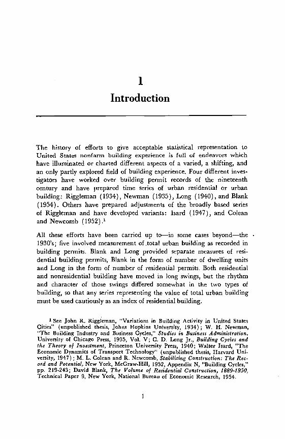
Introduction
The history of efforts to give acceptable statistical representation toUnited States nonfarm building experience is full of endeavors whichhave illuminated or charted different aspects of a varied, a shifting, andan only partly explored field of building experience. Four different inves-tigators have worked over building permit records of the nineteenthcentury and have prepared time series of urban residential or urbanbuilding: Riggleman (1934), Newman (1935), Long (1940), and Blank(1954). Others have prepared adjustments of the broadly based seriesof Riggleman and have developed variants: Isard (1947), and Coleanand Newcomb (1952).'
All these efforts have been carried up to—in some cases beyond—the1930's; five involved measurement of ,total urban building as recorded inbuilding permits. Blank and Long provided separate measures of resi-dential building permits, Blank in the form of number of dwelling unitsand Long in the form of number of residential permits. Both residentialand nonresidential building have moved in long swings, but the rhythmand character of those swings differed somewhat in the two types ofbuilding, so that any series representing the value of total urban buildingmust be used cautiously as an index of residential building.
1 See John R. Riggleman, "Variations in Building Activity in United StatesCities" (unpublished thesis, Johns Hopkins University, 1934); W. H. Newman,"The Building Industry and Business Cycles," Studies in Business Administration,University of Chicago Press, 1935, Vol. V; C. D. Long Jr., Building Cycles andthe Theory of Investment, Princeton University Press, 1940; Walter Isard, "TheEconomic Dynaniics of Transport Technology" (unpublished thesis, Harvard Uni-versity, 1947); M. L. Colean and R. Newcomb, Stabilizing Construction: The Rec-ord and Potential, New York, McGraw-Hill, 1952, Appendix N, "Building Cycles,"pp. 2 19-243; David Blank, The Volume of Residential Construction, 1889-1950,Technical Paper 9, New York, National Bureau of Economic Research, 1954.
1

Introduction
While these variant measures of our urban building history werebeing designed, overlapping series of measures were being worked Out byother investigators for urban building activity since 1900, 1915, and 1920.Utilizing all available building permit materials and other information onconstruction, and using the technique of stratification of universe andchecking against controlling census-derived figures, David Wickens devel-oped a highly regarded and widely used residential 'building series for theperiod Working independently, Chawner elaborated a residen-tial building series going back to 1900 on the strength of permit recordsand Dodge contract information.3 Official statistical agencies in the De-partments of Labor and Commerce have developed residential and otherbuilding series carried back to 1915 and maintained currently. For theperiod 1889-19 19, the official agencies have adopted the Blank residentialbuilding series, while, conversely, Blank and his National Bureau asso-ciates, Grebler and Winnick, have accepted the Wickens-Labor Depart-ment permit-derived residential unit series for the post-1919 period.4The 1889-1939 composite will be termed BLS-NBER series.
Meanwhile, Simon Kuznets and Robert Galiman developed over-allconstruction series going back quinquennially to 1840 and available on asmoothed annual basis since 1869. These measures are 'based upon decen-nial totals for construction materials produced in this country and des-tined for domestic use, with annual interpolators derived from annualseries of particular types of building materials or quinquennial statecensus recordings of construction materials produced. The Kuznets andGailman series show different rhythms and characteristics for somedecades of the nineteenth century.5
The biases of all building-permit-derived series are now well known.Until recent years, those series, in effect, provided a record of buildingexperience only within the covered central cities of metropolitan areas.Since building permits were not generally required in suburban and
2 See final version as presented in David L. Wickens, Residential Real Estate,New York, NBER, 1941, pp. 41-50.
L. 3. Chawner, The Residential Building Process, Washington, 1939, andConstruction Activity in the United States 1915-1937, Washington, 1938.
" Nonfarm Housing Starts 1899-1958, Department of Labor, Bull. 1260, 1959.5 See R. Galiman, "Commodity Output, 1839-1899," in Trends in the Ameri-
can Economy in the Nineteenth Century, Studies in Income and Wealth, Vol. 24,Princeton for NBER, 1960; Simon Kuznets, Capital in the American Economy:Its Formation and Financing, Princeton for NBER, 1961, Apps. B and C.
2

Introduction
satellite communities within metropolitan areas, the series did not catchnoncentral-city building until those communities were annexed. Adequateallowance for the effect of annexations has always been difficult to make.6In addition, the patterns of building in central Cities and in satellite andrural areas may diverge significantly. Adequate allowances for divergentrhythms of building in cities of different size classes have proved difficultto make. Finally, building has spread outward from city centers at a ratefaster than the permit-reporting network has been 'broadened. Theseweaknesses have led to continual upward revisions of the more recentbroadly based building-permit series. The permit-derived series for thenineteenth century, with their limited coverage, patently rest on insecurefoundations.
The biases which run through construction-material-derived seriesare of a different character. First, amplitudes are dampened because ofthe substantial volume of construction materials used for maintenanceand repair. Second, building and construction materials are used not onlyfor building but also in other ways about which detailed information isknown only for more recent years. Lumber is used for crates and boxes,as a fuel, in shipbuilding, and for manufacture of wooden products; bricksare used for sidewalks, Street surfacing, and for underground construc-tion.7 Third, annual interpolators for the building-material series arecomparatively scant and not representative during most of the nineteenthcentury. Finally, the most important building materials, lumber and brick,were produced through most of that century typically in small establish-
6 For example, analysis of the results of the National Housing Inventory of1956 disclosed that sizable undercoverage, which eluded the reporting permit net-work, was traceable to "failure to treat annexations correctly." At least during theperiod 1950-56, "surveys of non-permit housing starts seriously underestimatedactual starts in non-permit areas." See Progress Report on Improvements in Con-struction Statistics, Census Bureau, Feb. 12, 1960, pp. 2 and 6.
In 1912 some 74 per cent of lumber was used in construction while 26 percent was used to produce box crates, furniture, vehicles, and other wooden prod-ucts (Lumber and Timber Products, Works Progress Administration, GPO, May1938, p. 108). In the nineteenth century wood was still widely used for heatingand industrial fuel. Ohio railroads in 1858 used 209,416 cords of wood and816,675 tons of coal (Ohio Executive Documents, Part 2, 1858, p. 584). In 1892it was noted that "the utilization of brick for street paving has opened a newmarket for brick and created a distinct industry. Within the past few years thou-sands of miles of streets have been paved with this material throughout the West"(Mineral Resources of the United States, Bureau of Mines, GPO, 1892, p. 723);V. S. Clark, History of Manufacturers in the United States, McGraw-Hill for Car-negie Institution of Washington, 1929 ed., Vol. II, p. 494.
3

Introduction
ments, many of which were operated only part time to meet local needs.8The output of such establishments is in all countries difficult to evaluatestatistically in reliable annual measurements.9 The fourteenfold growthrecorded by Gailman in the production of construction materials between1840 and 1900 thus reflects in part the drying up of local productionfacilities, not fully reflected in our records.1° Since the historic process ofindustrialization moved unevenly throughout the century, the patterns ofmovement of the census-recorded segment of the industry may give adeceptive account of total building activity.
At this juncture, new sources of information must be utilized. Onehelpful source may be found in the little-used "vintage" report of theHousing Census of 1940, which developed estimates of the decade inwhich 92 per cent of the enumerated dwelling units were erected.11
8 "In the years preceding the Civil War the production process differed butlittle from the methods used since earliest historical times," with brick often beingproduced by hand methods and improvised kilns "at the building site" (A. J. Tas-sel, D. W. Bluestone, Mechanization in the Brick Industry, WPA, 1939, p. 4).The 1880 Census Weeks Report commented (p. 27): "Brickmaking in many sec-tions of the country is carried on upon a small scale and in a desultory way; thenumber of employees is small and the subdivisions of labor are of little importance."Even though William Haber reported that the brick industry between 1870 and1890 had developed from "small scattered undertakings to a commercial enter-prise of large proportions," still the Bureau of Mines in its 1895 report noted thedifficulty of keeping a directory of• producers up-to-date owing ". . . to the largenumber of plants, the constant establishment of new yards and the abandonment ofold ones" (William Haber, Industrial Relations in the Building Industry, Cam-bridge, Mass., Harvard University Press, 1930, p. 25, Mineral Resources, 1895,p. 817).
Right up to the present time," notes a Swedish account, in the late 1920's,"the brick-making industry, included in the Industrial Statistics since 1873, onlyrepresents part of the total output of the country, as bricks are still largely manu-factured as a home industry subsidiary to agriculture." Data with regard to thesawmill industry and the allocation of sawmill products to building and other useswas found too imperfect, before 1896, to warrant making annual estimates of valueof construction using a "materials-used" base (E. Lindahi, E. Dahlgren, K. Kock,National Income of Sweden 1861-1930, London, P. S. King & Son, 1937, Part I,p. 177; Part II, p. 186).
10 Gallman records a fourteenfold rise in construction materials used (mil-lions of constant dollars) from 87 in 1839 to 1,224 in 1899. This contrasts with asixfold rise in the recorded Construction labor force from 269,000 gainful workersin 1839 to 1,640,000 in 1899. Gallman, "Commodity Output, 1839-1899," pp.30, 63.
11 See use of vintage returns by M. Reid, "Capital Formation in ResidentialReal Estate," Journal of Political Economy, Apr. 1958, pp. 135 if.
4

Introduction
Another helpful source is the Continuous census reporting of the decadeincrements of occupied dwelling units which, with appropriate adjust-ments for vacancy and shrinkage, should correspond in some fashion withestimated new residential production. The census decennial counts ofincremental growth of urban population, occupied dwellings, and non-farm labor force will, for any one decade, correspond to residential build-ing only with a substantial margin of error, but the growth over a stretchof decades should aid in judging the adequacy of any set of decade hous-ing estimates.
Reliable decade totals of new residential production cannot, however,be derived from the census alone. We need to use independent measuresas well, in permit-reporting urban areas. Another measure has recentlybecome available owing to the discovery of a new stretch of hithertounutilized building and real estate data for an entire north central state,Ohio, available without lapses and with full coverage from 1857 to 1914.Annual increments (smoothed by a moving average) in the assessed valueof town and city real property were found to correlate closely with annualstatewide building values, permitting a projection of building back to1840. We also have available for ten years in the middle seventies andearly eighties an annual count, by number and value, of buildings in Ohiolost or demolished. This information sheds light on building shrinkagerates and thus helps to reconcile total production estimates with realizedincrements in standing structures.
Originally, the intention was to use the Ohio and other availablematerials to extend backward by a half-century the BLS-NBER series,which begins in 1889. Those estimates were regarded as sufficiently wellestablished, in spite of the well-known general weaknesses of permit-derived statistics. However, our first efforts to utilize the new materials forextrapolation disclosed an appreciable gap between the aggregate of"starts" for the decades between 1890 and 1910 as measured in the BLS-NBER series and as projected by our materials. The series seemed toseriously overestimate production in the 1890's and to underestimateproduction in the 1900's. Yet, quite clearly, the estimates for the twodecades could not be adjusted on the desired scale without upsetting thewhole pattern of decade levels and the secular trend running throughthe pattern. Nor could we build up an annual time series for the decadespreceding 1890 and pin it to a level that involved a serious overestimate.A continuous long series was required. Since other information also indi-cated that the BLS-NBER series tended to underestimation, the task of ageneral revision of our nationwide residential building statistics was under-
.5

Introduction
taken, beginning with the task of extending statistical coverage backwardin time.
The work of revision and extension is limited in this study to prepa-ration of annual nationwide estimates of the number of new housekeepingpermanent dwelling units erected. Our work of statistical revision andextension is also limited to preparation of estimates that will yield validknowledge about long-swing movements. We did not find it necessary toachieve the high degree of accuracy in year-to-year measures that wouldbe important for analysis of the short business cycle. Hence we haveutilized methods of statistical adjustment designed to achieve tolerableaccuracies in measures of growth trend and long swings, but which maynot do justice to short cyclical movements.
6
2
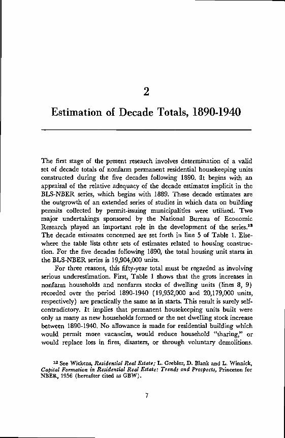
Estimation of Decade Totals, 1890-1940
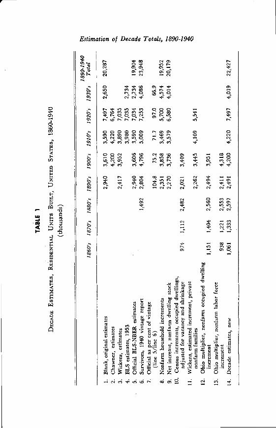
The first stage of the present research involves determination of a validset of decade totals of nonfarm permanent residential housekeeping unitsconstructed during the five decades following 1890. It begins with anappraisal of the relative adequacy of the decade estimates implicit in theBLS-NBER series, which begins with 1889. These decade estimates arethe outgrowth of an extended series of studies in which data on buildingpermits collected by permit-issuing municipalities were utilized. Twomajor undertakings sponsored by the National Bureau of EconomicResearch played an important role in the development of the series.'2The decade estimates concerned are set forth in line 5 of Table 1. Else-where the table lists other sets of estimates related to housing construc-tion. For the five decades following 1890, the total housing unit starts inthe BLS-NBER series is 19,904,000 units.
For three reasons, this fifty-year total must be regarded as involvingserious underestimation. First, Table 1 shows that the gross increases innonfarm households and nonfarm stocks of dwelling units (lines 8, 9)recorded over the period 1890-1940 (19,952,000 and 20,179,000 units,respectively) are practically the same as in starts. This result is surely self-contradictory. It implies that permanent housekeeping units built wereonly as many as new households formed or the net dwelling stock increasebetween 1890-1940. No allowance is made for residential building whichwould permit more vacancies, would reduce household "sharing," orwould replace loss in fires, disasters, or through voluntary demolitions.
12 See Wickens, Residential Real Estate; L. Grebler, D. Blank and L. Winnick,Capital Formation in Residential Real Estate: Trends and Prospects, Princeton forNBER, 1956 (hereafter cited as GBW).
7
TA
B%
.E 1
DE
CA
DE
EST
IMA
TE
S, R
ESI
DE
NT
IAL
UN
ITS
BU
ILT
, UN
ITE
D S
TA
TE
S, 1
860-
1940
(tho
usan
ds)
1890
-194
018
60's
1870
's18
80's
1890
's19
00's
1910
's19
20's
1930
'sT
otal
1.B
lank
, ori
gina
l est
imat
es2,
940
3,61
03,
590
7,49
72,
650
20,2
87
2.C
haw
ner,
est
imat
es4,
200
4,22
06,
764
3.W
icke
ns, e
stim
ates
2,41
73,
952
3,89
07,
035
4. B
LS
estim
ates
, 195
33,
980
7,03
52,
734
5.O
ffic
ial B
LS-
NB
ER
est
imat
es2,
940
3,60
63,
590
7,03
42,
734
19,9
04
6.Su
rviv
ors,
194
0 vi
ntag
e re
port
1,49
22,
804
4,79
65,
009
7,25
34,
086
23,9
487.
Off
icia
l as
per
cent
of
vint
age
(lin
e 5/
line
6)10
4.8
75.2
71.7
97.0
66.9
8.N
onfa
rin
hous
ehol
d in
crem
ents
2,35
13,
858
3,46
95,
700
4,57
419
,952
9.N
et in
crea
se, n
onfa
rm d
wel
ling
stoc
k2,
270
3,73
63,
579
6,58
04,
014
20,1
7910
.C
ensu
s in
crem
ents
, occ
upie
d dw
ellin
gs,
adju
sted
for
vac
ancy
and
shr
inka
ge97
41,
112
2,48
22,
021
3,40
911
.W
icke
ns, e
stim
ated
incr
emen
t, pr
ivat
eno
nfar
m f
amili
es2,
262
3,44
54,
109
5,54
1
12.
Ohi
o m
ultip
lier,
non
fari
n oc
cupi
ed d
wel
ling
incr
emen
t1,
151
1,40
42,
560
2,49
43,
951
13.
Ohi
o m
ultip
lier,
non
farm
labo
r fo
rce
incr
emen
t93
81,
221
2,55
32,
411
4,31
814
.D
ecad
e es
timat
es, n
ew1,
061
1,33
32,
597
2,49
14,
200
4,22
07,
497
4,01
922
,427

Estimation of Decade Totals, 1890-1940
SOURCE, BY LINE
1. Blank, The Volume of Residential Construction, pp. 11, 59.2. Chawner, Residential Building, p. 13.3. Wickens, Residential Real Estate, p. 54.4. Construction During Fiue Decades) Dept. of Labor, Bull. 1146, 1953, p. 3.5. Non-Farm Housing Starts 1889-1958, Dept. of Labor, Bull. 1260, 1959,
p. 15.6. Sixteenth Census of the United Stages, 1940, Housing, Bureau of the
Census, Vol. III, Part 1 (1943), Table A-i, p. 9 (except for exclusionof three months of 1940 as disclosed in the report in same series Housing,1945, p.3).
8. Grebler, Blank, and Winnick, Capital Formation in Residential RealEstate, p. 82.
9. Ibid., p. 86.10. See Table 13.11. Wickens, Residential Real Estate, p. 55.
12 to 14. See Table 12 for 1860-1900 and Section 2, below, for later decades.
The starts total thus presupposes an implausible deterioration in housingstandards over the fifty-year period.13
Second, critical scrutiny of later bench-mark studies indicates that,around the fourth decade of this century, our established permit-derivedresidential building statistics have tended to understatement ranging upto 20 per cent.14 It is reasonable to hold that this tendency to under-statement did not begin abruptly in 1940. Third, concrete indications ofunderstatement are offered by the findings of the vintage statistics of the1940 and 1950 Censuses. Owners, managers of residential buildings, or
13 Though the tables were presented in GBW and commented on extensively,the issue of the consistency between cumulated starts and stock aggregates was by-passed. It was explicitly recognized that between 1890 and 1930, before the ten-dency to convert had allegedly grown strong, new calculated starts only slightlyexceeded growth in households and dwelling stock (GBW, p. 88). The slight ex-cess (of 988,000 units of housing stock) "reflects the net effects of demolitions,conversions and other changes in the housing stock" (p. 88). As Margaret Reidhas pointed out, ". . . there will be a tendency to overestimate the number of con-versions or to underestimate the number of demolitions in order to account forthe net change in number of non-farm dwellings indicated by decennial censuses"(Reid, "Capital Formation," n 23).
14 Between 1930 and 1956, BLS estimates of housing starts "probably ac-counted . . . for between 70-80 per cent. . ." of the reported net change in unitsstanding after liberal allowances for conversions and demolitions" (Grebler andS. Maisel, "Determinants of Residential Construction," mimeographed memo forCommission on Money and Credit, Oct. 1959, IV- 17).
9

Estimation of Decade Totals, 1890-1940
knowledgeable neighbors were requested in the 1940 Census to disclosethe year built of the original structure in which the surveyed residentialunits were located. The returns were presented by years for the firstdecade, by five-year intervals for the second decade, and thereafter bydecade totals back to 1859. Vintage information was obtained for 92 percent of the surveyed residential units.
Collecting decade totals for dwelling units for which year-built infor-mation was furnished, the vintage record (line 6, Table 1) as of the 1940census enumerated 23,948,000 dwelling units in the 1940 stock as locatedin surviving structures originally erected after 1890. This total cannotbe compared, without adjustment, with the 19,904,000 units estimatedin the BLS-NBER series. Vintage attributions represent standing stockand thus include converted units, units transferred from the farm sectorto the nonfarm and nonpermanent dwellings excluded from the startscategory. The vintage attributions likewise do not include units builtbetween 1890 and 1939 but destroyed or demolished, or for which avintage report was not filed. Specified estimates under these headings aregiven in Table 2.
TABLE 2
1940 CENSUS VINTAGE REPORT ON
DWELLING UNITS BUILT, 1890-1940
(thousands)
Number nonfarm housing units originally constructed, 1890-1940(unadjusted 1940 Census report) 23,948
1. Minus number of converted units included 2,436
2. Minus number of nonpermanent ineligible units included 147
3. Minus farm units transferred to nonfarm stock 150
4. Plus units built between 1890 and 1940 and destroyed or demolished 1,000
5. Plus units built after 1890 and not reporting vintage 1,805
Total adjusted 24,020
NOTE: For detailed explanation of the five adjustments, see the Appendix.
10

Estimation of Decade Totals, 1890-1940
The largest task of estimation involved the breakdown of convertedunits, numbering 3.18 million, and nonreporting units, numbering 2.35million, into structures of origin erected before or after 1890. Some tend-ency was found for age to influence the distribution in both cases. Sur-viving older units are more prone to conversion, and it seems plausiblethat owners or managers of surviving older units are more likely to beignorant of vintage. The evidence on hand indicated a stronger tendencyfor conversion to :be correlated with age. We accepted the results of regres-sion analysis, which put 76.7 per cent of the 1940 stock of converted unitsinto the post-1890 vintage category. With less clear-cut evidence, thevintage category of nonreporting units was adjusted by the same percent-age. With other adjustments, this produced an estimated total of 24,020,-000 permanent housekeeping nonconverted dwelling units built between1890 and 1940, or 20.7 per cent more than the number in BLS-NBERseries. A detailed explanation of the adjustments set forth in Table 2 isgiven in the Appendix.
The table and Appendix presuppose that the vintage attributions arecorrect, or that errors of judgment or estimation as to year built wererandom. What are the probabilities of correct information and the direc-tion of probable bias? In their rejoinder to Margaret Reid's use of vintagedata along lines indicated above, Grebler, Blank, and Winnick pointed tothe unreliability of vintage attributions for particular years.15 For theindividual years of the 193 0's, the reports follow closely the index patternsderived from permit data (see Chart 13) except for a tendency to over-estimation in 1930 and 1935. This is a manifestation of the well-knownbias by which census age distributions cluster at multiples of 5. Censusrespondents should ordinarily have known the year-built of residentialproperties less than ten years old. Probably at least half the propertieswere resided in by people responsible for their original construction; onlya small proportion would have passed though more than a second set of
15 "Second, and more importantly, the number of dwelling units reported tothe 1950 Census as being in structures built in, say, 1925 or even 1941 bears onlya vague resemblance to the number of dwelling units actually built in 1925 or1941" (Grebler, Blank, and Winnick, "Once More: Capital Formation in Resi-dential Real Estate," Journal of Political Economy, 1959, p. 613).
11

Estimation of Decade Totals, 1890-1940
owners.'6 Those owners, in turn, would have purchased with awarenessof age.
If the decade of the l93O's passes muster, so can the decade of the1920's. The total reported 7,253,000 units falls well within the range ofthe volume of starts estimated independently by Blank and by Wickens(see Table 1, lines 1 to 5). A respectable proportion of the propertieswere still lived in by people who would have had direct information aboutthe timing of original construction.
As we turn to earlier decades, confidence in vintage attributiondiminishes. The proportion of original or even second owners would havebeen much smaller. Age has a marked bearing on value, and abstracts ofdeeds available for scrutiny by owners or held by them usually indicateyear of construction. But not all buyers commonly inspect abstracts, andcensus enumerators were instructed to accept estimates deemed reliable.'7Under these circumstances, a bias toward over- or under-age estimationis possible. We can only check the returns for indications of any con-sistent bias cumulated in one direction.
16 Tabulation of "year moved into" data from owner occupants in the 1960Census shows that about half the owner occupants in Wisconsin have resided inthe properties for ten years or longer. The average length of occupancy of anowner-occupied home is seven to ten years. (E. M. and R. M. Fisher, Urban RealEstate, New York, Henry Holt, 1954, p. 232). Nationwide census tabulation in1960 of the urban population (including renters) showed that 23.9 per cent ofthe urban population had resided in the "present house" for ten years or longeror had always lived in the "same house." Census of Population: 1960. GeneralSocial and Economic Characteristics, United States Summary, Final Report PC (1)-IC GPO, 1962, Tables 71 and 72.
17 The enumerators were instructed to find out the year built from an owneroccupant, a well-informed neighbor, or a tenant. If the exact answer was not ob-tainable, the enumerator was instructed to enter "the approximate year based onavailable information and observation" (1940 Census, Housing, Vol. H, Part I,p. 195). The Census Bureau conducted no formal evaluation for this item. Theresponsible head of the Housing Division of the Bureau asserted: "From a quali.tative standpoint we believe that this item [year-built data] is subject to ratherlarge response errors, particularly for renter occupied units that have been builtmore than ten years prior to the date of the Census" (letter from D. B. Rathburn,Mar. 24, 1962). Systematic check of year-built census returns by census tracts inMilwaukee revealed that the returns tallied very closely with year-built returns ofthe independent real property inventory carriedout between 1934 and 1936 (H. G.Berkman. The Delineation and Structure of Rental Housing Areas, University ofWisconsin Commission Reports, Vol. IV, 1956, p. 31, n. 5). So also a closelyaligned vintage pattern was found between the 202 Cities (1934-6) and 64 cities(1934) canvassed in the real property inventory surveys and the 1939 urban censusenumeration (Peyton Stapp, Urban Housing, A Summary of Real Property Inven-tories, 1934-1936, WPA, GPO, 1938).
12
Estimation of Decade Totals, 1890-1940
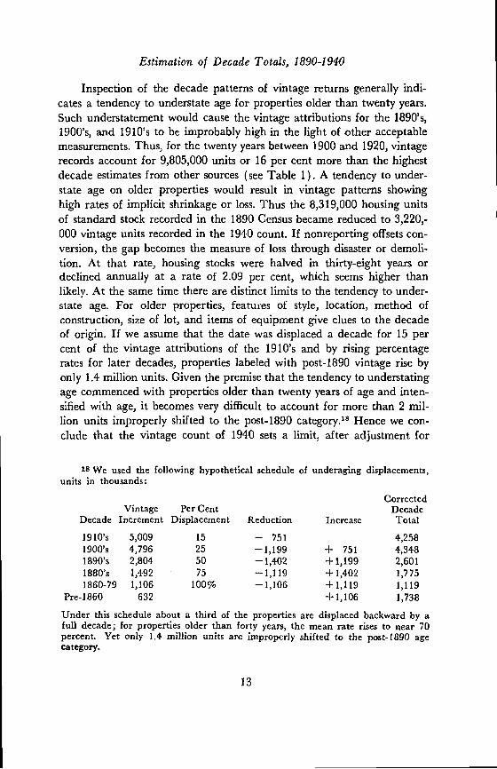
Inspection of the decade patterns of vintage returns generally indi-cates a tendency to understate age for properties older than twenty years.Such understatement would cause the vintage attributions for the 1890's,1900's, and 1910's to be improbably high in the light of other acceptablemeasurements. Thus, for the twenty years between 1900 and 1920, vintagerecords account for 9,805,000 units or 16 per cent more than the highestdecade estimates from other sources (see Table 1). A tendency to under-state age on older properties would result in vintage patterns showinghigh rates of implicit shrinkage or loss. Thus the 8,319,000 housing unitsof standard stock recorded in the 1890 Census became reduced to 3,220,-000 vintage units recorded in the 1940 count. If nonreporting offsets con-version, the gap becomes the measure of loss through disaster or demoli-tion. At that rate, housing stocks were halved in thirty-eight years ordeclined annually at a rate of 2.09 per cent, which seems higher thanlikely. At the same time there are distinct limits to the tendency to under-state age. For older properties, features of style, location, method ofconstruction, size of lot, and items of equipment give clues to the decadeof origin. If we assume that the date was displaced a decade for 15 percent of the vintage attributions of the 1910's and by rising percentagerates for later decades, properties labeled with post-1890 vintage rise byonly 1.4 million units. Given the premise that the tendency to understatingage commenced with properties older than twenty years of age and inten-sified with age, it becomes very difficult to account for more than 2 mil-lion units improperly shifted to the post-1890 category.18 Hence we con-clude that the vintage count of 1940 sets a limit, after adjustment for
18 We used the following hypothetical schedule of underaging displacements,units in thousands:
CorrectedVintage Per Cent Decade
Decade Increment Displacement Reduction Increase Total
1910's 5,009 15 — 751 4,2581900's 4,796 25 —1,199 + 751 4,3481890's 2,804 50 —1,402 +1,199 2,6011880's 1,492 75 —1,119 +1,402 1,7751860-79 1,106 100% —1,106 +1,119 1,119
Pre-1860 632 +1,106 1,738
Under this schedule about a third of the properties are displaced backward by afull decade; for properties older than forty years, the mean rate rises to near 70percent. Yet only 1.4 million units are improperly shifted to the post-1890 agecategory.
13

Estimation of Decade Totals, 1890-1940
comparability, of underestimation in the BLS-NBER series of around 20per cent, or some 4 million units for the fifty-year period, 1890-1940, or atthe very least 10 per cent and 2 million units; and that any independentlysupported estimate falling within that range should be acceptable.
How should the BLS-NBER decade estimates for 1890-1940 be cor-rected for a tendency to underestimation ranging between 10 and 20 percent? All decade totals could be scaled upward at a uniform rate. Thatwould, however, presuppose the forces that biased the starts count to haveworked uniformly over the decades concerned. A uniform bias is, how-ever, unlikely in view of the varying coverage of permit-reporting areasand the unequal and shifting currents of rural, urban, and central citygrowth over the surveyed period. Hence, adjustment for underestimationhas been based upon review, decade by decade, of the available evidenceand judgment of the likely shifts in decade growth patterns.
For the decade of the 1930's we can accept with slight modificationthe verdict of the 1940 vintage report. For these relatively new properties,age estimates by census respondents should be reliable. Implicit annualrates of vintage production tallied closely with starts patterns (see Chart13). Few of the newer vintage units of the thirties would have been con-verted, unreported for age, or wiped out by fire or demolition. Accord-ingly, we subtract from the vintage report oniy an appropriate allowancefor nonpermanent or "ineligible" units, or for units built in the 1930's andtransferred from the farm to the nonfarm sector.'9
19 In an unpublished note on "Naigles' Reconciliation of BLS Decade Startswith Census Stock Increments and Vintage Attributions," Moses Abramovitz al-lowed the following magnitudes (my estimates for the same items are in paren-thesis).
Adjustments for Structures Built in the Thirties (thousands)1. Conversions 70.8 (0)2. Temporary and nonhousekeeping 141.6 (59)3. Reclassification from farm sector 91.0 (8)4. Demolition and other loss — 4.0 (0)5. Nonreporting vintage —67.0 (0)
I follow Abramovitz in estimating that items 1, 4, and 5 substantially offset eachother. My estimate for item 2 is the total number of ineligible units classifiedunder the "other dwelling place" category and with a vintage traced back to thethirties. I have scaled down the possible reclassification from the farm sector to8,000 units because the 1940 Census Count disclosed that only 8.2 per cent of therural-farm dwelling unit 1940 stock was built during the 1930's. If transference tothe nonfarm sector was unaffected by age, then only some 8.2 per cent of the trans-ferred rural-farm units were built in the thirties (see p. 95 below).
14

Estimation of Decade Totals, 1890-1940
For the decade of the 1920's we have available two independentefforts at measurement by Wickens and by Blank (7,035,000 and 7,497,-000 units, Table 1, lines 1, 3). The sample of building-permit data util-ized by both investigators was of the same magnitude, and both utilizedrefined estimating techniques. Blank commented quite properly that"external evidence affords no possibility of determining with any precisionthe degree of error in either of the two series."20 However, since permitdata tended to underestimation, it seemed reasonable to take the higherof the two estimates. Since the tendency to urban sprawl was inhibited inthe twenties by the building splurge in central cities, permit statistics inthe twenties were much closer to target than in the decade of the thirtieswith its marked drift of building outside the permit reporting-system.21
For the 1890's we have available decade estimates derived fromBlank and from our own projections of the Ohio data (see Chapter 3).For checking, these results may be contrasted with census increments inhousehold or dwelling stocks both unadjusted or as adjusted by Wickensor by myself (see Table 1). For various reasons the Ohio projectionsseemed preferable as an estimation basis for the 1890's. The Ohio-derivedestimate tallies very closely with results reached by Wickens with theoriginal census returns. Blank's sample of reporting systems started out inthe 1890's with only 25 cities covering only 14.5 per cent of the nonfarmpopulation; by 1900 sampled cities numbered 68 but with a populationcoverage of only 24.0 per cent.22 The reporting sample was obviously toolimited to permit refined estimation by urban size classes and regions. Atthe same time, the rapid growth of the sample may have generated bias.Finally, a basic assumption of the Blank expansion procedure is highlyquestionable, namely, that "nonf arm nonurban residential constructionbears the same relationship to the increase in rural nonfarm population
20 Blank, Volume of Residential ConstTuction, p. 59.
21 The acceleration of urban sprawl in the thirties is indicated by a varietyof evidence. Thus population growth—and by inference residential building—wasmaintained during the thirties for the "rural ring" in metropolitan areas, thoughspecific urban population growth fell off sharply (see GBW, p. 100). Likewise the1940 Census vintage reports show that the urban segment of nonfarm buildingwas steadily maintained within 3 percentage points of 80 per cent for the fourdecades after 1890 but fell to 63.4 per cent in the thirties. Since permit report-ing systems provided weak coverage of building in the small towns or rural en-virons of central cities, the disparate behavior of permit-reporting systems in thetwenties and thirties is explicable.
22 Blank, Volume of Residential Construction, p. 35.
15
Estimation of Decade Totals, 1890-1940
that urban construction bears to the increase in urban population."23 Thisoverstates rural building by not allowing for the smaller urban-familysize; it understates rural building on the other hand by not allowing forreplacement building which would be unrelated to population growth.With these limitations, the Blank estimate for the 1890's seemed lessacceptable than our Ohio-derived estimates. If the Blank level wereaccepted and given the decade patterns that seemed indicated, the aggre-gate level of building output for the eighty years after 1860 would beexcessive in the light of end-1939 dwelling stocks and probable loss rates.
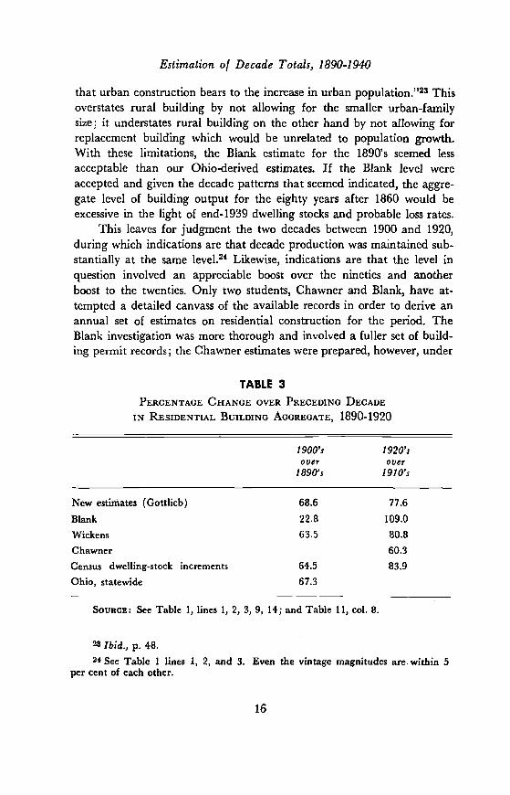
This leaves for judgment the two decades between 1900 and 1920,during which indications are that decade production was maintained sub-stantially at the same level.24 Likewise, indications are that the level inquestion involved an appreciable boost over the nineties and anotherboost to the twenties. Only two students, Chawner and Blank, have at-tempted a detailed canvass of the available records in order to derive anannual set of estimates on residential construction for the period. TheBlank investigation was more thorough and involved a fuller set of build-ing permit records; the Chawner estimates were prepared, however, under
TABLE 3
PERCENTAGE CHANGE OVER PRECEDING DECADE
IN RESIDENTIAL BUILDING AGGREGATE, 1890-1920
1900'sover
1890's
1920'sover
1910's
New estimates (Gottlieb) 68.6 77.6
Blank 22.8 109.0
Wickens 63.5 80.8
Chawner 60.3
Census dwelling-stock increments 64.5 83.9
Ohio, statewide 67.3
SOURCE: See Table 1, lines 1, 2, 3, 9, 14; and Table 11, col. 8.
Ibid., p. 48.24 See Table 1 lines 1, 2, and 3. Even the vintage magnitudes are. within 5
per cent of each other.
16

Estimation of Decade Totals, 1890-1940
very competent direction. The Blank estimates level out at 3,600,000 unitsfor the 1900's, the Chawner at 4,200,000 (see Table 1, lines 1, 2). As ithappens, our Ohio-derived estimates for the decade of the 1900's runvery close to Chawner's (4,135,000, Table 1, average of lines 12 and 13).The bias for underestimation of permit statistics would argue for theuse of the higher of two independent sets of permit-derived estimates.Finally, such use in conjunction with the levels previously fixed for thenineties and the twenties yields a plausible set of decade-shift patterns(see Table 3).
For the five decades surveyed, our aggregate estimated productionis 22,427,000 units or 12.8 per cent over the BLS-NBER aggregate. Ourupward adjustments allow for about two-thirds of the gap between thevintage and the BLS-NBER aggregates.
17

3
Estimation of Decade Totals, 1860 -90
We turn to estimation of decade production before 1890. For this task,the vintage report and urban-permit statistics give little guidance as tosecular drift or decade shiftings. It is fortunate that new data have be-come available for nearly the entire second half of the nineteenth century.
The number and value of new buildings erected in the state of Ohio,by county, were reported annually from 1857 through 1914, together withmarriage and real estate conveyance data. The nature of the statisticalfindings, the adjustments to which they were subjected, and the testsmade of their validity will be reported on more fully in a monographnow in preparation.
Original collecting agents of the building schedule were local town-ship assessors working under the direction of county auditors in a programof statistical reporting inaugurated by state law in Ohio in 1857. Localassessors, as a matter of official duty, would keep records of new building(and losses) for the purpose of maintaining property assessment rolls. Wefirst ran audited tapes of reported county residential building andadjusted these tapes for deficient returns. The reported totals behaveplausibly when contrasted with increments of assessed real property, orwhen laid out as time series. A variety of tests indicate that the data weuse here have a high degree of reliability. Reports on nonpublic construc-tion were in general compiled with more care than were reports on tax-exempt construction; and statistics, such as we deal with here, of dwellingunits by number bypass the adjustments needed to allow for either thechanging value of the dollar or shifting appraisal standards. The figuresoriginally reported were adjusted only to allow for incomplete returns,for obvious errors in printing or arithmetic, and for conversion from a
18

Estimation of Decade Totals, 1860-90
record of "building completed" to a record of "building performance"for a uniform reporting period.25
Table 4 indicates that the state is qualified to serve as a basis fornational estimation. The state was well settled by 1850 and respondedfully to the building throbs of the middle-passage years of the nineteenth
TABLE 4
SELECTED INDEXES OF COMPARABILITY, OHIO AND THE UNITED STATES,
1840-1910
Percentage GrowthDecennially inPopulationa
Ohio U.S.
UrbanPopulation
as Percentageof Total
Population
PercentageShare ofNonf armin Total
Labor Force
Total Non/armIncome perNon/armWorker(dollars)
All Urban All Urban Ohio U.S. Ohio U.S. Ohio U.S.
1840 22 21 356 437
1850 30 190 36 92 12 15
1860 18 65 36 75 17 20
1870 14 71 23 59 26 25
1880 20 51 30 43 32 28 37 34 551 572
1890 [5 47 26 57 41 35
1900 13 32 21 36 48 40 56 44 609 622
1910 15 33 21 39 56 46
SOURCE: Richard A. Easterlin, "Interregional Differences in Per Capita In-come, Population, and Total Income, 1840-1950," in Trends in the AmericanEconomy in the Nineteenth Century, App. A, pp. 97 ff.; Ohio Population, State ofOhio, Dept. of Industrial and Economic Development, 1960, Table 3; Bureau ofCensus, 1950 Census, Ohio, pp. 35-36, Statistical Abstract 1920, p. 32; andHistorivd Statistics of the United States, 1789-1945, 1949, p. 25, Table B13-23.
a For decades closing in the specified year.
25 Terminal dates of reporting years were either unspecified or shifted fromJuly 1, May 1, and April 12. The practice was to make a spring survey (earlyor late) of what in effect was construction undertaken in the preceding year andcompleted by the reporting date. Some small structures could, however, have beencommenced and completed within a reporting year ending May 1 or July 1. Itwas not possible to allow for this, and hence our calendar year allocations mayhave some "backward" bias. The adjustment for incomplete returns compensatedfor counties omitted from statewide returns. The adjustment was usually madeby linear interpolation. Until the reporting system broke down in 1910-14, only afew counties were omitted from published returns in any given year.
19

Estimation of Decade Totals, 1860-90
century. Through that period, industry in Ohio was diversified and urbanpopulation was well distributed by size-class of city. In 1850 the statecontained 8.54 per cent of the population of the country, 8 percent ofmanufacturing establishments, and 7 per cent of nationwide real estatevalue. Decennial rates of growth of urban population were falling bothin Ohio and in the nation; and the share of total urban population wasrising both in Ohio and in the nation. Table 4 shows that in terms ofnonfarm income per nonfarm worker, Ohio by 1880 had moved closeto the national average.
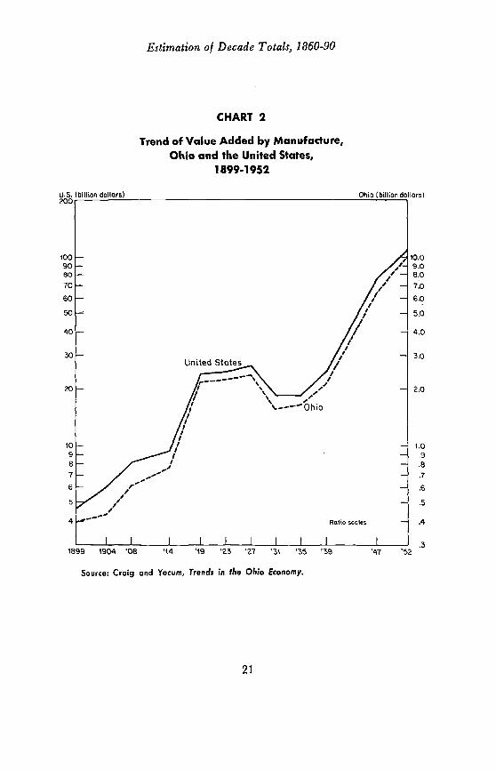
Craig and Yocum in a recent study note: "Over the past 50 years,Ohio's growth in population, industry, commercial development, trans-portation facilities, agricultural output—nearly any economic measurethat can be taken—has kept pace almost precisely with the United Statesas a. whole." Their three charts substantiating this finding are repro-duced here as Charts 1, 2, and 3. They continue: "The reason there has
CHART 1Trend of Population in Ohio and the United States, 1900-50
U.S. (millions)
20
9
8
7
6
5
41950
Ohio C millions)
1900 1910 1920 1930 1940.
Source: Cr&g and Yocum, Trends in the Ohio Economy.
Estimation of Decade Totals, 1860-90
CHART 2
Trend of Value Added by Manufacture,Ohio and the United States,
1899-1952
21
1899 (904 '08 '(4 '(9 'Z3 '2? '3S '35 '39 '47 '52
Source: Craig and Yocum, Trends in the Ohio Economy.

Estimation of Decade Totals, 1860-90
CHART 3
Trend of Electrical Power Production inOhio and the United States,
1900-51
Source: Craig and Yocum, Trends in Ihe Ohio Economy.
22
10.09.08.07.0
6.0
5.0
4.0
3.0
2.0
1.0.9.8
.7
.6
.5
.4
.3
.2
KWH)
30.0
20.0
.1

Estimation of Decade Totals, 1860-90
been a remarkable parallelism between Ohio arid the United States asa whole lies not only in Ohio's central location, but in the combination ofvaried resources and circumstances which have permitted Ohio to developa diversification of basic economic activities which closely mirrors that ofthe United States at large."26 The study included an average index ofdeviation for 1950 showing divergence by selected states from the nationaldistribution of employment by major industrial groups. The details forOhio are shown in Table 5.
TABLE 5
PEBCENTAGE DISTRIBUTION OF EMPLOYMENT, MAJOR INDUSTRYGROUPS, Orno AND THE UNITED STATES, 1950
Deviation ofPer Cent Ohio Percentageof Total from U.S.
U.S. Ohio Percentage
Agriculture, forestry, and fisheries 12.6 7.1 5.5
Mining 1.7 1.0 — 0.7Manufacturing 26.3 37.1 +10.8Transportation, communication, public
utilities, and construction 14.1 13.2 — 0.9Trade 19.0 18.5 — 0.5Service and professional 18.3 16.2 — 2.1Finance 3.5 2.8 — 0.7Government 4.5 4.1 — 0.4
Total 100.0 100.0 21.6
SOURCE: Craig and Yocum, Trends in the Ohio Economy, Table 1, p. 12.
In terms of cyclical sensitivity, Ohio manufacturing is more concentratedthan the national aggregate is in durable goods production (nationwide,41.8 per cent of value added against Ohio, 59.3 per cent in 1939).Nevertheless, the estimated average per cent of compensable labor forceunemployed in 1933 was nearly identical in Ohio (28.7 per cent) withthe nationwide total (27.5 per cent). The state has also shown employ-ment trends almost parallel to those of the United States (see Chart 4).
26 P. G. Craig, J. C. Yocum, Trends in the Ohio Economy, Bureau of Busi-ness Research, Ohio State University, Res. Mon. 79, 1955, p. 1.
23

Estimation of Decade Totals, 1860-90
CHART 4
Covered Employment in Ohio and the United States,1938-5 1
24
1938 '39 '40 '41 '42 '43 '44 '45 '46 '47 '48 '49 '50 '51
Source: Craig and Yocum, Trends in the Ohio Economy, p. 29.

Estimation of Decade Totals, 1860-90
Some structural characteristics of nationwide and Ohio dwellings,1890-1940, are given in Table 6. By and large, the layout of characteristicsis reassuring. The distribution by number of rooms is modal at the five-to six-room house, though there are fewer small units and more largerunits in Ohio. The per cent of rented dwellings was somewhat less than
TABLE 6
STRUCTURAL CHARACTERISTICS OF OHIO AND UNITED STATES DWELLINGS,
1890-1940
Percentage Distribution Percentage Distribution1939 Nonfarm Dwelling Nonfarm Dwelling
Stock by: Ohio U.S. Stock by: Ohio U.S.
Number of Rooms City-size class (continued)I 2.3 3.7 Built 1900-40 54.8 73.42 5.4 8.4 Built before 1900 39.4 20.63 9.9 14.2 In converted units 7.5 7.64 13.8 18.15 23 20 7
Rural farm, entire 16.6 25.8
6 24:6 17:7 Built 1900-40 99.5 69.57 9.8 7.4 Built before 1900 55.7 26.58 or more 9.9 8.4 In converted Units 3.8 2.9Not reporting 1.0 1.3 In PMD, entire 62.6 553
Period built Built 1900-40 72.8 72.31935.39 4.7 7.9 Built 1879-1900 16.4 14.1
1930-34 4.0 6.0 Built before 1879 6.2 5.01925-29 12.4 13.51920-24 10.5 11.1 Per cent of nonfarm units1910-19 18.0 17.0 rented1900-09 17.3 16.2 1930 48.50 54.561890-99 11.5 9.5 18901880-89 7.0 5.11879 or earlier 8.9 5.9 Percentage 1940 nonfarmNot reporting 5.5 8.0 units, 1-family detached 62.0 55.2
Internal featuresIn converted Units 10.2 9.3 Average value, allConverted to residential 1.1 1.4 nonfarm dwellingsWith private bath and 1930 $5,138 $5,022
flush toilet 60.3 57.6 1900 J,671 1,951With central heating 62.1 46.0
Average value, mortgagedCity-size class nonfarm dwellings
Urban, Outside PMDa 21.4 22.7 1890 $2,366 $3,250Built 1900-40 57.3 68.7 1920 5,012 4,938Built before 1900 34.3 22.9In converted Units 12.1 13.3 Average value, nonfarni
Rural nonfarm, home mortgageOutside 16.0 21.9 1890 $ 879 $1,293
SouRcE: Wickens, Residential Real Estate, pp. 80-85, Tables A-I, A-3; Sixteenth Censu.s, 1910,Housing, Characteristics by Type of Structure, Tables A-I to A-5, pp. 3 if., 270-289; Dept. ofInterior, Census Division, Report on Farms and Homes, 1896; Census Bureau, Wealth, Debt.and Taxation, GPO, 1907, p. 17.
APMD principal metropolitan district.
25
Estimation of Decade Totals, 1860-90
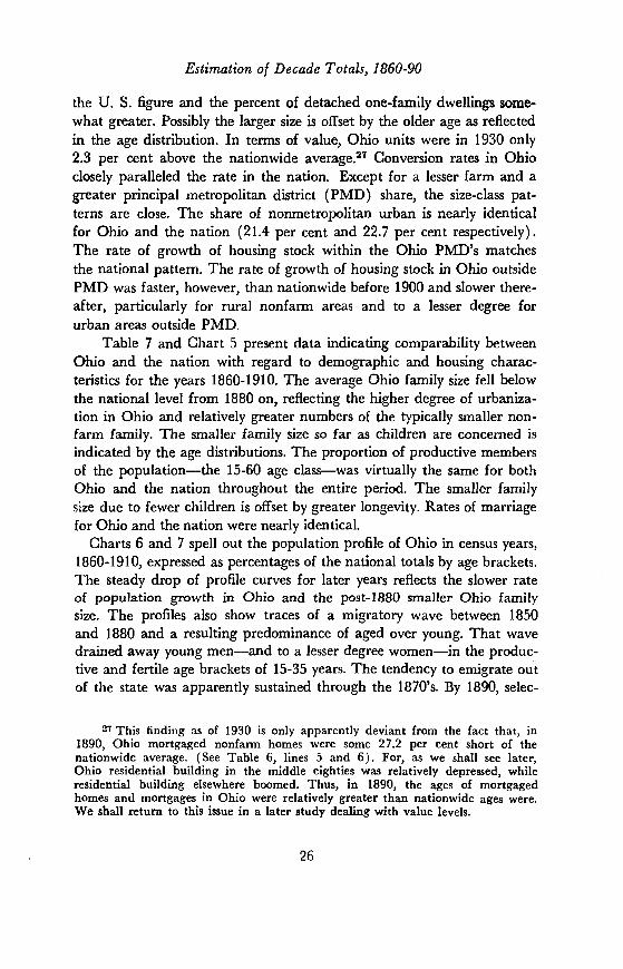
the U. S. figure and the percent of detached one-family dwellings some-what greater. Possibly the larger size is offset by the older age as reflectedin the age distribution. In terms of value, Ohio units were in 1930 only2.3 per cent above the nationwide average.27 Conversion rates in Ohioclosely paralleled the rate in the nation. Except for a lesser farm and agreater principal metropolitan district (PMD) share, the size-class pat-terns are close. The share of nonmetropolitan urban is nearly identicalfor Ohio and the nation (21.4 per cent and 22.7 per cent respectively).The rate of growth of housing stock within the Ohio PMD's matchesthe national pattern. The rate of growth of housing stock in Ohio outsidePMD was faster, however, than nationwide before 1900 and slower there-after, particularly for rural nonfarm areas and to a lesser degree forurban areas outside PMD.
Table 7 and Chart 5 present data indicating comparability betweenOhio and the nation with regard to demographic and housing charac-tens tics for the years 1860-1910. The average Ohio family size fell belowthe national level from 1880 on, reflecting the higher degree of urbaniza-tion in Ohio and relatively greater numbers of the typically smaller non-farm family. The smaller family size so far as children are concerned isindicated by the age distributions. The proportion of productive membersof the population—the 15-60 age class—was virtually the same for bothOhio and the nation throughout the entire period. The smaller familysize due to fewer children is offset by greater longevity. Rates of marriagefor Ohio and the nation were nearly identical.
Charts 6 and 7 spell out the population profile of Ohio in census years,1860-1910, expressed as percentages of the national totals by age brackets.The steady drop of profile curves for later years reflects the slower rateof population growth in Ohio and the post-1880 smaller Ohio familysize. The profiles also show traces of a migratory wave between 1850and 1880 and a resulting predominance of aged over young. That wavedrained away young men—and to a lesser degree women—in the produc-tive and fertile age brackets of 15-35 years. The tendency to emigrate outof the state was apparently sustained through the 18 70's. By 1890, selec-
27 This finding as of 1930 is only apparently deviant from the fact that, in1890, Ohio mortgaged nonfarm homes were some 27.2 per cent short of thenationwide average. (See Table 6, lines 5 and 6). For, as we shall see later,Ohio residential building in the middle eighties was relatively depressed, whileresidential building elsewhere boomed. Thus, in 1890, the ages of mortgagedhomes and mortgages in Ohio were relatively greater than nationwide ages were.We shall return to this issue in a later study dealing with value levels.
26

TA
BLE
7
DE
MO
GR
AP
HIC
CO
MPA
RIS
ON
OF
OH
IO A
ND
UN
ITE
D S
TA
TE
S, 1
860-
1910
t.. 0 0 I
Ave
rage
Siz
e Fa
mily
POPU
LA
TIO
N B
ET
WE
EN
AC
ES.
IN
YE
AR
S(p
er c
ent)
.
Est
imat
edN
et0
to 1
415
to 6
060
and
Ove
rO
hio
asO
hio
asO
hio
asO
hio
asIn
terc
ensu
sPe
r C
ent
Per
Cen
tPe
r C
ent
Per
Cen
tM
igra
tion'
Ohi
oU
.S.
of U
.S.
OhL
oU
.S.
of U
.S.
Ohi
oU
.S.
of U
.S.
Ohi
oU
.S.
of U
.S.
(tho
usan
ds)
1860
5.39
5.28
102.
141
.20
40.5
010
1.7
54.2
555
.05
98.6
4.54
4.45
102.
018
705.
115.
0910
0.4
39.2
639
.20
100.
155
.21
55.7
798
.95.
535.
0310
9.9
1880
4.98
5.04
98.8
—12
.918
904.
684.
9394
.932
.95
35.5
292
.758
.66
58.0
310
1.1
8.39
6.43
130.
441
.919
004A
04.
7692
.430
.85
34.4
789
.461
.21
59.1
010
3.5
7.94
6.43
123.
477
.719
104.
204.
5492
.528
.19
32.1
387
.762
.89
61.1
010
2.9
8.92
6.77
131.
720
7.7
PER
CE
NT
AG
ED
IST
RIB
UT
ION
AN
D M
AR
ITA
L S
TA
TU
S, W
OM
EN
15
YE
AR
SA
ND
OV
ER
Perc
enta
ge R
ate
of M
arri
age,
Sing
leM
arvi
edFe
mal
es, 1
5 Y
ears
and
Ove
r
Ohi
o as
Ohi
o as
Ohi
o as
CE
NSU
SPe
r C
ent
Per
Cen
tPe
r C
ent
YE
AR
Ohi
oU
.S.
of U
.S.
Ohi
oU
.S.
of U
.S.
Ohi
oU
.S.
of U
.S.
1890
32.4
31.8
101.
856
.556
.899
.43.
126
3.07
210
1.7
1900
31.1
31.2
99.6
57.2
57.0
100.
33.
006
3.14
795
.519
1028
.929
.797
.359
.558
.910
1.1

Os
C,
xg,(100
C,

Per cent8.5
4.0 -
Estimation of Decade Totals, 1860-90
CHART 6Ohio Male Population as Per Cent of United States
Male Population, by Age, Census Years,1860-1910
I I 1.1 I I I I I I
5 10 15 20 25 30 35 40 45 50 55 60 65 Over65
Souree: 1860, 8th Census, Population, pp. 370-371, 596-597. 1870, 9th Census, VitalStatistics, pp. 580-593. 1890, 11th Census, Population, Part II, pp. 72-73, 2-5. 1900, 12thCensus Population, Part II, pp. 78-79. 1910, 13th Census, Vol. 1, Population, pp. 303, 394.
29
1860
8.0
7.5
7.0
6.5
6.0
5.5
1890
Under I

Per cent8.0
.7.5
7.0
6.5
6.0
5.5
5.0
4.0 —
Estimation of Decade Totals, 1860-90
CHART 7
Ohio Female Population as Per Cent of United StatesFemale Population, by Age, Census Years,
1860-1910
Under I 5 10 15 20 25 30 35 40 45 50 55 60 65 Over65
30
Some as for Chart 6
1890
4.5

Estimation of Decade Totals, 1860-90
tive age emigration had become mild, and by 1900 and 1910 it had dis-appeared. Net emigration was apparently reversed during the 1870's(see Table 7) with steadily rising net intercensus immigration. Immigrantsapparently account for the Ohio tendency to a higher average age.
These materials indicate that while the state may readily serve as abase for national projection, allowance must be made for certain peculiarfeatures of the state's economic development. Thus, in terms of percentagedecennial growth of urban population, inspection of Chart 8 shows threenonconforming decade movements. The decline in the rate of urbangrowth between 1850 and 1860 was much steeper for Ohio than forthe nation. During the sixties, Ohio urban population growth, unlikethat of the nation, reversed trend. During the eighties, Ohio urbanpopulation had little of the booming growth that marked the nationalcourse, indicating that the comparative intensity of long urban-buildingswings experienced in Ohio cannot be mechanically projected to thenational scene.
While Ohio's urban growth and industrial development broadlymatched in intensity the nationwide movement, its agricultural populationand settlement showed comparatively little growth after the Civil War.Hence, the state became more highly urbanized and industrialized thanthe nation as a whole. This, in turn, along with selective age migration,helped produce a relatively smaller average household size and a house-hold age composition different from the nation's.
Three alternative sets of census increments are available to projectOhio building experience into nationwide aggregates: urban population,nonf arm dwelling stock, and nonf arm labor force. The first two arederived from the census enumeration of population and dwellings; thethird, from the census enumeration of occupations. The three projectionbases represent different facets of the process of economic and demo-graphic growth. Growth of the employed nonf arm labor force wouldpresuppose additional households and dwellings. If the rates of householdformation per unit of nonfarm labor force are the same in Ohio and inthe nation, and if additional nonfarm households are similarly appor-tioned between urban and nonfarm rural locations in Ohio and thenation, then all three projection bases should yield identical returns. Butdivergences in returns may reflect not only real differences but also inac-curacies or biased enumeration or estimation of the three projection basesfor Ohio and the nation. First, the projection bases are examined forreal differences in relative rates of growth and, second, they are assessedfor statistical biases.
31

Estimation of Decade Totals, 1860-90
CHART 8
32
1900-10
Decennial Per Cent Change in Urban Population,Ohio and the United States,
1840- 1910
1840 1850 1860 1870 1880 1890-50 -60 -70 -80 -90 -1900
Source: Table 4.

Estimation of Decade Totals, 1860-90
The relative rates of dwelling-unit increment per unit of labor-forceand increments in Ohio and the nation are presentedin Table 8, along with actual nationwide increments in occupied non-farm dwellings and national increments projected on Ohio rates (lines15-19). Divergences between nonfarm dwellings and nonfarm labor-forceincrements were largely offset in the aggregate. For the first four decades,projection of nationwide housing increments on Ohio rates yielded figuressmaller than those with the shortage concentrated in the first decade.During the 1900's, Ohio rates generated considerably larger figures thanwere realized nationally. In part, the decade variations reflect real diver-gences between Ohio and nationwide rates of household formation perunit of nonfarm labor force; in part, they reflect statistical inaccuraciesin our nationwide measures of agricultural housing and labor. Enumera-tion of the nonfarm labor force in the U. S. Census was uncertain foragricultural workers, sometimes included in the category of general orunclassified workers. The Ohio enumeration may have been differentfrom the national especially for the southern states with their fluid insti-tutional patterns of farm operation.28
Another term in our comparison, occupied dwellings, was also diffi-cult to adjust for farm dwellings by methods that could be applieduniformly in Ohio and the nation. Increments in farm dwellings can begauged chiefly by increments in either farm establishments or farm laborforce. The first measure is biased in the nationwide count by the breakupof plantations in the South, offset only in part by the rise elsewhere oflarge agricultural production units. Hence, the number of farms expandedafter 1870 at a faster rate than farm families or farm dwellings did.On the other hand, hired farm labor was not consistently classified fromcensus to census or possibly even for Ohio and the nation.29
The variations shown in Table 8, lines 13 and 14, between Ohioand nationwide rates of household increments per unit of urban popula-tion are much greater than the corresponding measure per unit of non-farm labor force. The urban measure yields sizable underestimates forthe first two decades. The cumulative tendency to underestimation wasgenerated by higher rates of household formation per unit of urban
28 From 1860 to 1910, farm labor force grew from 6,207.6 to 11,591.8, or by86.7 per cent. Farms by number grew from 2,044 to 6,406, or by 213.4 per cent.Historical Statistics, 1949, Series D37, p. 72, Series Ki, p. 278.
20 For the nation as a whole, farm laborers accounted for 51.5 per cent ofthe agricultural labor force in 1860 and 39.2 per cent in 1910. Ohio shares wereabout half as large.
33

Estimation of Decade Totals, 1860-90
TABLE 8
NET HOUSEHOLD FORMATION BY NONFARM LABOR-FORCE INCREMENT
AND BY URBAN-POPULATION INCREMENT, OHIO AND THE STATES,
BY DECADE, 1860-1910(units in thousands)
Increment 1860's 1870's 1880's 1890's 1900's
1. Nonfarm labor-force increment2. Ohio3. United States
106.01.525.4
153.03,016.7
276.34,491.5
258.74,521.7
368.36,892.9
4. Nonfarm dwelling-unit increment5. Ohio6. United States
53.9952.1
59.8901.0
129.52,110.5
111.92,023.8
171.82,941.7
7. Urban-population increment8. Ohio9. United States
282.53,685
347.84,228
479.47,976
488.28,054
666.811,839
10. Dwelling Units as per centof increment
Nonfarm labor force11. Ohio (line 5/2)12. United States (line 6/3)Urban-population increment13. Ohio (line 5/8)14. United States (line 6/9)
50.8662.42
19.0825.84
25.9929.87
11.4421.51
46.7846.99
27.0226.46
45.2544.76
22.9325.13
46.6542.68
25.7624.85
IS. National dwelling incrementprojected on Ohio rates
16. Laborforce (line llxS)
17. Percent of actual (line 16/6)
18, Urban population (line 9x13)
19. Per cent of actual (line 18/6)
776
81.5
703
73.8
81490.3
48453.7
2,105
99.8
2,155
102.!
1,956
96.7
1,847
91.3
3,216
109.4
3,050
103.7
SouRcE: Tables 9 and 10; Eleventh Census, 1890, Population, Part I, p. 913; ThirteenthCensus, 1910, Population, Part I, p 1287. Line 5 derived from increment of total occupieddwellings less the farm increment of dwellings.
population in Ohio than in the nation. The average ages of Ohio urbanpopulation over the decades and the whole sweep of its age profiles werehigher than those in the nation. More crucially, too, rates of urbanizationper unit of growth in the nonfarm rural population were higher in Ohiothan in the nation. New villages arose more slowly, and existing villageswere more rapidly converted to urban status in Ohio than in the nation.Hence, rates of nonfarm housing growth per unit of urban-populationincrement would be lower in Ohio than in the nation. For these reasons,urban population was not used as a projection basis in our final calcula-tions.
Granted that the statistical biases of the other two projection basesare less serious, are they satisfactory in other respects? Would rates ofnew residential building in Ohio per unit of our projection bases be
34
Estimation of Decade Totals, 1860-90
equal to nationwide rates? If so, it would imply that demolition andshrinkage rates were the same in Ohio and the nation, and that the sharesof replacement construction to net growth were the same. Substantially,this is indicated by the scrappy evidence available. The relative share ofthe more durable brick and masonry structures was nearly the same inOhio (13.3 per cent) as in the nation (13.9 per cent), to judge by theproportions of standing residential stock of those types in Theaverage age of housing stock in Ohio was probably somewhat under thenational average age in the earlier decades of the projection, but con-tinuous western settlement balanced off the newer regions against theolder seaboard regions and probably brought the Ohio average dwellingage—and hence rates of shrinkage—into rough correspondence withnationwide levels. Such correspondence is indicated, at least, by the lastquarter of the nineteenth century. The existing national shrinkage esti-mate for the three decades before 1920, stated in terms of per cent ofdwelling production, amounted to 11.5,8.2 and 7.1 per cent, respectively.Residential shrinkage rates in Ohio on the basis of annual Counts between1873 and 1884 probably approached 4 per cent in the 1870's and 5.5-6.0per cent in the 1880's (see below, page 000). At any rate, the divergencebetween shrinkage rates, if these fragmentary data are to be trusted,would affect only a small fraction of total production. Hence, projectionof Ohio replacement rates upon nationwide totals represents a fairlyserviceable expedient, considering our needs, our objectives, and ourmargin of accuracy.
The work of projecting Ohio building experience into nationwidetotals resolved itself into laying out three basic sets of decade aggregates:(1) Ohio and nationwide increments of nonfarm dwellings; (2) Ohioand nationwide increments of nonfarm labor force; and (3) new Ohioresidential nonfarm production. In each category, estimation was involvedin fixing the farm-nonfarm boundary. For dwellings, it could be gaugedin the decades after 1890. Comparison of increments in farm establish-ments by number of establishments and number of farm families disclosedthat farm-family increments were uniformly 25 per cent greater thanfarm establishment increments. The shrinkage factor was applied to farmestablishment increments before 1890. The details of the adjustment areset forth in Table 9. Estimation of the nonfarm boundary in the labor-force increments was confined chiefly to adjustments in the nationwide
30 Sixteenth Census of the United States, 1940, Reports on Housing, Vol. II,General Characteristics of Housing, by States, GPO, 1944, p. 68.
35

C-)
TA
BLE
9
CA
LCU
LAT
ION
OF
EST
IMA
TE
S, N
AT
ION
AL
NO
NFA
RM
DW
EL
LIN
G I
NC
RE
ME
NT
S, 1
860-
1910
(uni
ts in
thou
sand
s)
a 18
50-8
0:11
th C
ensu
s, 1
890,
Pop
ulat
ion,
Par
t I, p
. 913
.18
90-1
910:
13t
hb
from
His
tori
cal S
tatis
tics,
194
9, p
. 95,
E1-
5.C
ensu
s, 1
910,
Pop
ulat
ion,
Par
t I, p
. 128
7.
Adj
uste
d up
war
d on
bas
is o
f 18
70 C
ensu
s re
port
to in
clud
e sl
ave
dwel
lings
com
para
ble
with
Neg
ro d
wel
lings
of
late
rce
nsus
yea
rs.
d N
ot a
djus
ted
for
unde
rcou
nt, w
hich
pri
mar
ily in
volv
ed a
gric
ultu
ral p
opul
atio
n, n
ot c
over
ed b
y th
e fa
rm-d
wel
ling
adju
st-
men
t. e75
per
cent
of
valu
e of
act
ual i
ncre
men
t.Fr
om C
ensu
s re
cord
of
incr
emen
ts o
f fa
rm f
amili
es, a
ppro
xim
atel
y eq
ual t
o 75
per
cen
t of
farm
incr
emen
t. H
isto
rica
lSt
atis
tics,
194
9, S
erie
s H
89, p
. 174
.
Est
imat
ed
Cen
sus
Yea
rD
ecad
e
Dw
ellin
gC
ensu
sR
ecor
deda
Stoc
k
Incr
emen
tFa
rmSt
ockb
Act
ual
Incr
emen
tE
stim
ated
Incr
emen
t
Incr
emen
t,N
onfa
rmD
wel
lings
1860
5,62
8.6c
2,04
4.1
1870
186O
's7,
042.
8d1,
414.
12,
660.
061
646
2°95
2.1
1880
1870
's8,
955.
81,
913.
04,
008.
91,
349
1,01
2e90
1.0
1890
1880
's11
,483
.32,
527.
54,
564.
655
641
7e2,
110.
519
0018
90's
14,4
30.1
2,94
6.8
5,73
7.4
1,17
22,
023.
819
1019
00's
17,8
05.8
3,37
5.7
6,36
1.5
625
434f
2,94
1.7

Estimation of Decade Totals, 1860-90
count, designed to allow for the nonwhite-slave components of the south-ern labor force in 1860 and for the undercount of Negro labor in theSouth in 1870, as given in Table 10.
Estimation of Ohio residential dwellings erected were confined inthe main to computed allowance for the share in this total of farmdwellings, set forth in Table 11. The procedure was to utilize decadeincrements in number of farms (column 2) as an acceptable measure ofnet change in farm dwellings, with some allowance for replacement pro-duction of farm dwellings. A special study of the five least-urban Ohiocounties during 1900-10 indicated considerable farm residential-replace-ment building to cover losses from fire, demolition, or scrapping of olderbuildings.8' Accordingly, we presupposed that statewide replacementrates, as set forth in Table 11, column 4, applied to farm dwelling stocksand calculated an allowance for gross farm dwelling production (column6) and a parallel schedule of nonfarm residential production (column 8).
The details of the projection into nationwide housing estimates ofOhio nonfarm building rates, per unit of nonfarm-labor force and non-farm-dwelling increments, are set forth in Table 12. All decade turns innationwide dwelling production (Table 12, and Chart 9) are shared.Since the two multipliers yielded estimates close in pattern and level, andmany of the biases inherent in each should be offsetting,32 it seemedsensible to average the two estimates for projection purposes. The re-sulting level of decade estimates was adjusted upward slightly to fit thepreviously accepted estimates of 1900-20 (Table 12, line 7, and Chart 9).
The reliability of these decade estimates has been subjected to fourtests wholly or partly independent: the first checks for decade patternand level between 1860 and 1910; the second and third check over-alllevels of building between 1860 and 1940; the fourth checks the decadeof the eighties.
31 The five counties had a 1910 percentage of urbanization ranging between15.7 and 20.8. They contained, in 1910, 30,591 families and 13,028 farms. Overthe decade, total population fell by 3,452; urban population rose by 4,214; whilenonfarm, nonurban population fell by 3,835. The number of farms declined by866. Both farms and rural dwellings of 1900 shifted categories over the decade.Yet, over the decade, 6,751 new dwellings were erected. Replacement building onfarms is also indicated by the reported production of new barns and stables (3,093)and the increment (partly induced by price inflation) of value of building onfarms ($8.2 million) averaging $632 per farm.
32 Biases include: (1) possible nonuniformity by states in the administrationof census definitions and enumeration procedures; (2) allowance for farm dwell-
by 25 per cent rule (see p. 35) ;.. (3) delineation of agricultural laborerfrom "general laborer"; and (4) variation in the handling between Ohio andnationwide or between successive censuses of semiprivate households.
37

Estimation of Decade Totals, 1860-90
TABLE 10
FORCE, AND NONFARM, UNITED STATES AND OHIo,BY DECADE, 1860-1910
1860 1870 1880 1890(1) (2) (3) (4)
1900(5)
1910(6)
United SLatesLABOR FORCE RECORDED
AllFarmNonfarni
9,425,133a 12,924,951 17,392,099 23,318,1834,288,984b 6,263,394 7,713,875 9,148,4485,1 36,1 49e 6,661,557 9,678,224 14,169,755
29,073,23310,381,76518,691,468
38,167,33612,582,99725,584,339
OhioAllFarmNonfarm
640,043 840,889 994,475 1,287,101302,798 397,613 398,188 414,544337,245 443,276 596,287 872,557
1,545,952414,662
1,131,290
1,919,055419,423
1,499,632
1860's 1870's 1880's 1890's 1900's
United StatesAllNonfarin
DECADE INCREMENTS OF RECORDED LABOR FORCE
3,499,818 4,467,148 5,926,084 5,755,0501,525,408 3,016,667 4,491,511 4,521,733
9,094,1036,892,871
OhioAllNonfarin
200,846 153,586 292,626 258,851106,051 159,011 276,270 258,753
373,108368,342
SOURCE, BY COLUMN
(1) Eighth Census, 1860 Population, p. 399, pp. 656-680, for only free personsover 15 years old. Number of students was subtracted from Census figure.
(2) Ninth Census, 1870, Compendium, p. 594, corrected for understatement of1870 Census. See Sixteenth Census, 1940, Comparative Occupation Statt.cticsfor the United States, 1870 to 1940, p. 104.
(3)—(5) Twelfth Census, 1900, Occupations at the Twelfth Census, pp. L andXCII.
(6) Thirteenth Census, 1910, Classified Index to Occupations, p. 41 and Popu-lation, Vol. 4, p. 125.
Notes: Technical Explanation of 1860 Adjustmenta Correction for 1860 Census was made as follows:1. Number of students was subtracted from census figures.2. To Count slaves, we took number of slaves by sex, 15 years and over:
male, 1,082,563; female, 1,074,748 (Eighth Census, p. 595). The number ofgainfully occupied slaves was estimated by multiplying the above figures by 0.75for male, 0.35 for female. These figures were added to the revised censusfigure 1.
Justification of choosing 0.75 and 0.35 as multipliers: For the years 1890,1900, and 1910, we have 0.79, 0.84, and 0.87 for males and 0.36, 0.41, and 0.55for females, 10 years-and-over age class. (Negro Population in the U.S. 1790-1915, Bureau of Census, 1918, p. 504.)
38
Estimation of Decade Totals, 1860-90
The percentage might be much higher for slaves in 1860, 15 years-and-overage class. But, for our purpose, it is necessary to estimate the total number ofgainfully occupied persons in the same terms, because Ohio had no slaves in thatyear. Therefore, projecting back from the figures of 1890, 1900 and 1910, andtaking account of difference in age class, the figures 0.75 and 0.35 were chosen.
b Ccl. line I minus ccl. 1, line 3.C To estimate the nonfarm slave population, the following steps were taken:1. We estimated the number of gainfully occupied urban slaves by multi-
plying the total estimated number of slaves in col. 1 by 0.067, which was theestimated fraction of the total slave population living in urban communities(Gunnar Myrdal, An American Dilemma, New York, 1944, P. 183).
2. We estimated gainfully occupied, nonfarm, nonurban slaves by multiply-ing the estimated gainfully occupied urban population by 1.29, calculated asfollows: the nationwide figures of urban and rural population, and persons inagricultural pursuits for the years 1910 and 1860, and farm population for 1910were taken from Historical Statistics, 1960. Then nonfarm, nonurban populationfor 1910 was calculated by subtracting farm population from rural population.To get farm population for 1860, the number of persons argiculturally employedin 1860 was multiplied by ratio of farm population to number of persons agri-culturally employed in 1910. Nonfarm, nonurban population for 1860 was calcu-lated by subtraction.
The ratio of nonfarm, nonurban population to the urban population wascalculated—I .29. The underlying assumption is that the ratio of nonfarm, non-urban gainfully occupied persons to urban gainfully occupied persons is the sameas that of population.
Finally, the total number of nonagriculturally occupied persons was calcu-lated by adding the two figures, estimated above, urban slaves gainfully occupiedand nonfarm, nonurban slaves gainfully occupied, to the census figure.
1. The first test reduces to an attempt to build a valid set of estimatesof new residential production from the nationwide census returns ofoccupied dwellings by adjusting for uniformity and allowing for vacancyand replacement production. The details of the estimate are presented inTable 13. The first colunm presents the census returns, which were ad-justed for 1850 to 1860 to include slave dwellings to ensure compara-bility with post-1860 returns. The second column presents an estimated setof vacancy allowances. For the years 1900 and 1910 we use Chawner'svacancy estimates, which appear reasonable on the surface havingemerged from an exceptionally careful study of dwelling counts andfamily units.83 Vacancy rates for other census years were gauged to the
Chawner's vacancy estimates compare as follows with Wickens' (per cent):Chawner Wickens
1900 2.53 4.01910 3.49 5.0
(Chawner, Residential Building Process, p. 16; Wickens, Residential Real Estate,pp. 54 if.). The only nationwide time series of vacancy rates are those reportedby the decennial English censuses, 1801-1911. The successive high-low variationsrun to less than two percentage points and, considering the greater age of the
39

TA
BLE
11
DE
RIV
AT
ION
OF
OH
IO N
ON
FAR
M H
OU
SIN
G E
STIM
AT
ES,
BY
DE
CA
DE
, 186
0-19
10
Decade
,
Sta
tew
ide
Rep
orte
dN
ewD
wel
lings
(1)
Farm
Dw
elli
Incr
emen
tFa
rms
(2)
ng A
djus
tmen
t
Farm
Sto
ck,
Beg
inni
ngof
Dec
ade
(000
's)
(3)
Stat
ewid
eD
wel
ling,
Est
imat
edR
epla
cem
ent
Rat
e pe
r10
0(4)
Est
imat
edR
epla
cem
ent
of F
arm
s(3
)X (4)
(5)
Tot
alFa
rmA
djus
tmen
t(2
)+ (5)
(6)
Rep
lace
men
tIn
crem
ent
of N
ewPr
oduc
tion
(000
's)
(7)
Est
imat
edN
onfa
rmD
wel
lings
Prod
uced
(1)—
(6)
(8)
•1860's
89,490
16,064
179.9
4.58
8,239
24,303
19.5
65,187
1870's
126,365
51,236
196.0
6.73
13,191
64,427
33.4
61,938
1880's
181,390
4,241
247.2
8.13
20,097
24,338
47.7
157,052
1890's
177,196
25,289
251.4
5.55
13,953
39,242
40.0
137,954
1900's
254,120
—4,674
276.7
10.13
28,030
23,356
86.9
230,764
SOU
RC
E B
Y C
OL
UM
N
(1)
From
aud
ited
repo
rts,
adj
uste
d fo
r de
fici
ent r
etur
ns, o
f co
unty
aud
itors
, Ohi
o Se
cret
ary
of S
tate
Rep
orts
.(3
) B
urea
u of
Cen
sus,
13t
h C
ensu
s, A
gric
ultu
re, V
ol. V
, p. 6
8.(4
) D
eriv
ed b
y di
vidi
ng r
epla
cem
ent i
ncre
men
t of
new
pro
duct
ion
(col
. 7)
by th
e be
ginn
ing
deca
de to
tal d
wel
ling
stoc
k(f
rom
Cen
sus
of D
wel
lings
, Com
pend
ium
, 188
0, 1
910)
.(7
) D
eriv
ed b
y ad
ding
the
incr
emen
t of
farm
s (c
ol. 2
) pl
us n
onfa
rm d
wel
ling
units
incr
emen
t (T
able
8, l
ine
5) a
nd s
ub-
trac
ting
the
tota
l fro
m s
tate
wid
e re
port
ed n
ew d
wel
lings
(co
l. 1)
.

Estimation of Decade Totals, 1860-90
1900-10 level, taking account of the position of the census year in thebuilding cycle and the amplitude of movement of that cycle. The resultingvacancy estimates have little value in their own right and are used hereonly to adjust order of magnitudes. The determination of farm dwellingsinvolved the adjustment of farm increments (see Table 9) to allow forthe breakup of the plantation system.
Allowance for realistic estimates of conversion and shrinkage presentcomplex estimation problems. The 1940 vintage report, showing that only10.7 per cent of all dwelling units were converted (and this after a decadein which conversion activity was concentrated), indicates minimal decaderates of conversion, which were comparatively light in the decades be-tween 1860 and 1910. Grebler, Blank, and Winnick have already accepteddecade conversion allowances for later decades of the following percent-ages:34 1920's, 1.8; 1910's, 2.9; 1900's, 2.2; 1890's, 2.1. Accepting theindicated level, we accordingly specified the following pattern of conver-sion allowances, expressed as a percentage of dwelling production. Adownward trend is specified to allow for the factor of aging:35 1900's,2.2; 1890's, 2.0; 1880's, 1.8; 1870's, 1.6; 1860's, 1.4; 1850's, 1.2. Theshrinkage ratio is more variable and involves larger magnitudes thanconversion rates do. The BLS-NBER shrinkage estimates, drawn in largepart from informed guesses by Wickens, were as follows (stated in termsof per cent of dwelling production) 1930's, 15.0; 1920's, 8.3; 1910's,11.5; 1900's, 8.2; 1890's, 7.1.
English dwelling stocks and higher tenancy rates, the absolute levels are corn-parable with those estimated by Chawner (see the British rates as reproduced inH. W. Robinson, The Economics of Building, London, 1939, p. 106). The Chawnerestimates are also consistent with the carefully worked out 5.0 per cent estimateof Wickens for 1930 (based on an extensive analysis of 1930 and 1934 data,see pp. 22 if.) and the census reported gross vacancy rates of 6.5 per cent for1940 and 6.8 per cent in 1950, including vacant seasonal units and units heldfor absent households (see BLS-NBER, p. 776).
Capital Formation in Residential Real Estate, p. 329 (drawing largelyupon estimates by Wickens and Chawner).
The whole scale of conversion allowances from 1850 to 1940 is too low,since it accounts for only little more than half of the total stock of 3.3 millionconversion reported in the 1940 census count. But with present information thereis no way to distribute the shortage over the decades; the tendency to conversionprobably did not follow a uniform course. Hence, minimal conversion rates in linewith the Grebler, Blank, and Winnick estimates are accepted for the purposesof the above calculation.
36 See Capital Formation in Residential Real Estate, p. 329.
41

Estimation of Decade Totals, 1860-90
TABLE 12
DERIVATION OF UNITED STATES HOusING ESTIMATES BY USE OFOHIO MULTIPLIERS, BY DECADE, 1860-1910
(thousands)
DecadeOhio Multipliers 1860's 1870's 1880's 1890's 1900's Total
1. Non farm dwellings pro-duced in Ohio per1,000 nonfarm occu-pied dwelling incre-ments (Table 11, col.8, Table 8, line 5) 1,208.7 1,557.8 1,212.8 1,232.5 1,342.9
2. Nonfarm dwellings pro-duced per 1,000 non-farm labor force incre-ments (Table 11, col.8, Table 8, line 2) 615.0 404.8 568.4 533.2 626.5
3. Variant estimates, na-tionwide dwellingsproduction4. Line 1, above,
Table 8, line 6 1,150.8 1,403,5 2,559.6 2,494.3 3,950.5 11,558.4
5. Line 2, above,Table 8, line 3 938.1 1,221.2 2,552.9 2,410.9 4,318.3 11,441.4
6. Average 1,044.5 1,312.4 2,556.3 2,452.6 4,134.4 11,499.9
7. Average adjustedto Chawner 1900-19 levels 1,061 1,333 2,597 2,491 4,200 11,682
a Upward adjustment of 101.58 per cent.
The Ohio report of buildings lost, destroyed, or demolished showedthe following ratios to reported production of new dwellings in the sameyear.
Year Number Value Year Number Value1873 3.60 7.76 1878 4.32 4.621874 3.60 7.93 1880 4.69 5.971875 3.96 8.51 1881 5.25 14.401876 3.64 9.00 1882 5.40 6.521877 6.44 7.67 1884 6.30 12.40
For residential building, only the number estimates would be rele-vant. It would be expected that in the eastern states higher shrinkage
42

CHART 9
United States Decade Totals for New Dwellings,Three Variants, 1860-19W
1860 1870 1880 1890
Source: Table 12, lines 4, 5, 7; Table 13, cal. 8.
Estimation of Decade Totals, 1860-90
'+
4500
3500
labor force variant
Nonfarm dwelling variant
Accepted estimates
— —•—•—•— Adjusted census dwelling vortant
3000 —
2500 —
2000 —
1500 —
1000 —
500 —
I.' I I
1900 1910
43

TA
BLE
13
.4.
0 0 0 C-.
CA
LC
UL
AT
ION
OF
AD
JUST
ED
HO
USI
NG
PR
OD
UC
TIO
N F
RO
M C
EN
SUS
DW
EL
LIN
G18
60-1
910
Num
ber
Est
imat
edV
acan
cyA
djus
ted
Net
Cha
nge,
Non
farm
Con
vers
ion
and
Shri
nk-
Est
imat
edN
ew G
ross
Occ
upie
dV
acan
cyA
djus
ted
Farm
Rat
ePr
oduc
tion
Cen
sus
Dw
ellin
gsA
llow
ance
Stoc
kIn
crem
ent
age (7
)(8)
Yea
rDecade
(1)
(2)
(8)
(4)
(5)
NA
TIO
NW
IDE
1850
1840's
3,89
6.4a
103.
04,
013
1860
1850
's5,
628.
6b10
0.0
5,62
91,
616
446
1,17
01.
81,
191
974
1870
1860
's7,
042.
8c10
0.0
7,04
31,
414
462
1880
1870
's8,
955.
810
2.0
9,13
52,
092
1,01
21,
080
2.9
1,11
2
1890
1880
's11
,483
.310
4.0
11,9
422,
807
417
2,39
04.
72,
482
1900
1890
's14
,430
.110
2.5
14,7
912,
849
923
1,92
66.
02,
021
1910
1900
's17
,805
.810
3.5
18,4
293,
638
434
3,20
43,
409
9,99
8d
Cen
sus
Occ
upie
dD
wel
ling
Stoc
k
Vac
ancy
-A
djus
ted
Una
djus
ted
Dw
ellin
gFa
rmSt
ock
Incr
emen
t
Est
imat
ed N
ew G
ross
Pro
duct
ion
Alte
rC
onve
rsio
n an
dSh
rink
age
(12)
Yea
rD
ecad
e(9
)(1
0)(1
1)
NA
TIO
N E
XC
EPT
SO
UT
H
1850
1860
1840
's18
50's
2,34
3.5
3,64
5.2
2,41
3.8
3,64
5.2
437.
780
871
118
7018
60's
4,74
2.5
4,74
2.5
403.
164
118
8018
70's
5,94
8.7
6,06
7.6
702.
9
1890
1880
's7,
849.
78,
163.
725
0.4
1,91
7
1900
1910
1890
's19
00's
9,68
5.6
11,8
68.2
9,92
7.8
388.
712
,283
.614
7.0
1,44
32,
350
7,06
2
(1)
& (
9) 1
1th
and
18th
Cen
suse
s, P
opul
atio
n, P
art I
, pp.
913
, 128
7, r
espe
ctiv
ely.
(2)
See
text
, pp.
39f
f.(5
) T
able
9.
(7)
Det
erm
ined
by
subt
ract
ing
estim
ated
con
vers
ion
rate
s (p
. 41)
fro
m lo
ss r
ates
(p.
45)
.(1
.1)
Act
ual c
ount
of
num
ber
of f
arm
s, f
irst
dif
fere
nce.
Atis
trac
t of
Cen
sus,
15t
h C
ensu
s, 1
910,
p. 2
85.
"A
djus
ted
to in
clud
e sl
ave
dwel
lings
on
par
with
pos
t-18
60 c
ensu
s re
turn
s; c
alcu
late
d at
rat
e of
six
sla
ves
per
dwel
ling
(186
0ra
tes)
.b
Adj
uste
dby
187
0 C
ensu
s re
port
to in
clud
e sl
ave
dwel
lings
com
para
ble
with
pos
t-18
60 c
ensu
s re
turn
s.c
Not
adj
uste
d up
war
d fo
r 3.
3 pe
r ce
nt p
opul
atio
n un
derc
ount
, whi
ch d
id n
ot s
eem
to h
ave
affe
cted
the
farm
cou
ntor
the
nona
gric
ultu
ral
sect
or.
d18
60.1
910
only
.

Estimation of Decade Totals, 1860-90
rates would prevail. A rising tendency is indicated, though in part it mayreflect the cyclical movement in process. Other reports have shown thatshrinkage activity and demolition accelerates in the building boomphase.87 The years of the early eighties involved a marked boom. Inselecting shrinkage rates, consideration was also given to reported shrink-age rates elsewhere involving average annual replacement as a per cent ofnew residential production:38 Canada, 1920-1940, 19.4; Hamburg, 1885-1913, 13.2; Glasgow, 1873-1913, 45.0. The Glasgow rates as comparedwith the Hamburg rates disclose the influence of high average age of stockand slow rates of secular growth. Allowance must also be made for thetemporary character of nonfarm dwellings in the first round of settlement,the tendency to quick obsolescence, and relatively high rates of fire loss.In the later decades, demolition would accelerate in metropolitan com-munities owing to programs of highway and road building and revampingof city layout and design. 'In view of the Ohio demolition report, it seemedsafe to commence with a relatively low 3 per cent rate for the 1850's. Theprogression ends with the comparatively well-established rate of 15 percent for the decade of the 1930's. Intermediary rates were logarithmicallyinterpolated.
The crudeness of this procedure is recognized. Loss rates on totalhousing stock are probably a function of its average age, percentageshare of wood to masonry construction, and rate of new residential build-ing. There is no reason this interplay of influence should work out to asteady logarithmic progression of loss rates expressed as a fraction ofnew decade residential production. However, in the absence of intensiveresearch on loss rates and with uncertainty regarding absolute decadeloss levels, we have accepted the following percentages for the UnitedStates, 1850-1940: 1850's, 3.0; 1860's, 3.7; 1870's, 4.5; 1880's, 5.5; 1890's,6.7; 1900's, 8.2; 1910's, 10.0; 1920's, 12.3; 1930's, 15.0.
Table 13 also presents a similarly derived schedule of estimatedgross residential production for the entire nation except the South. Since
Thus Ohio decade replacement rates (see Table 11) were 8.13, 5.55, and10.13 per hundred dwellings of stock for the eighties, nineties, and nineteen-hundreds.
38 See A. K. Cairncross, Home and Foreign Investment 1870-1913, London,Cambridge University Press, 1953, p. 26; K. Hunscha, Die Dynamik des Bau-markt, Vierteljahreshefte Zur Konjunkturforschung, Sonderheft 17, Berlin, 1930,p. 60; 0. J. Firestone, Residential Real Estate in Canada, University of TorontoPress, 1951, pp. 382 if., 393 if. Chawner used demolition rates for the period1900-1936 ranging from 2.5 units per 10,000 persons in 1926 and 1928 to 6.0units in 1935 (Residential Building Process, p. 14).
45

Estimation of Decade Totals, 1860-90
nonsouthern farm increments corresponded more closely with the indi-cated real movement of agricultural population and its dwelling stocks,the farm-dwelling increments were unadjusted. This leads to a probablyexcessive spread between the national and nonsouthern or to an exagger-ated account of southern nonfarm dwelling production. Our estimatespresuppose that the nonsouthern part of the nation contributed only 71per cent of the nonfarm residential production between 1860 and 1910.The share, judging by measures of change in urban population of non-farm labor force, may well approach 80 per cent. A more precise regionalbreakdown of nonfarm residential building was not feasible within thelimits of this study.
The difficulty in reconciling the regional accounts underscores thecrudeness of our efforts to build up from census returns an estimate ofnew residential production. The aggregate level estimated falls shortby 13 per cent of the level projected by the two Ohio multipliers, whichwe have accepted. In part the shortage derives from our inability toadjust for underestimation in the census dwelling count between 1850-
More important is the decade pattern of movement as shown inChart 9, which conforms closely to the pattern of our accepted estimates.
2. A second test of these estimates provides a check on the aggregatelevel of residential 'building involved—11.7 million new nonfarm dwell-ings between 1860 and 1910. Between those years nonfarm populationto be housed grew by approximately 45.6 million.40 The average-size
Thus for 1900 and 1910 we used an unadjusted census count of 14,430,100and 17,805,800 occupied dwellings (see Table 13). The adjusted totals for house-holds used in Historical Statistics, 1949, H89-112, were 110.0 and 113.8 per centgreater.
40 For 1910, total nonfarm population was recorded by the Census at59,895,200. The problem is thus to build up an 1860 nonfann estimate. Of thetwo components of this estimate—urban and nonurban—the urban is recordedat 6,216,500. We build up the nonurban component by assuming that residentfarm population will show the same pattern of movement as total agricultural em-ployment (as taken from the occupations census). This is a more reliable basisfor projection than movement in number of farms. Farm-family size patterns prob-ably did not shift much over the fifty-year period. The numbers (in thousands)are as follows:
1860 1910Urban population 6,216.5 41,998.9Rural population 25,226.8 49,973.3Farm employment 6,207.6 11,591.8Nonfarm, nonurban population 8,048.6 17,896.3
(derived)Total nonfarm population 14,265.1 59,895.2
SouRcE: Historical Statistics, 1960, pp. 25-29, 63.
46
Estimation of Decade Totals, 1860-90
nonf arm household to be accommodated in 1910 was 4.24 persons,4'which would call for 10.76 million dwellings. If we allow for a 3.5 percent vacancy in the end stock in 1910 and if we specify a 6 per centshrinkage (for fire and loss) in post-1860 production as consistent withthe last tabulation, we emerge with a total new residential requirementover the fifty years of 11.8 million units.42 This is close to the magnitudeof our accepted decade levels.
3. A third check of over-all magnitudes is made possible by theHousing Census of 1940. Cumulation from 1860 to 1939 of all our esti-mates yields a total of 27.4 million dwellings. A comparison of that total(in thousands) with the known 1860 and end-1939 standing stock ofnonconverted eligible nonfarm dwellings is shown in the next tabulation.
1. Estimated new production nonfarm units 1860-1939 27,4182. Estimated 1860 nonfarm stock 3,167a
Total available (items 1 plus 2) 30,5854. Surviving eligible end-1939 standing stock of noncon-
verted nonfarm units 26211b
5. Gross disappearance (items 3 minus 4) 4,3746. Disappearance as per cent of new production (item
5 as per cent of item 1) 15.95Average of two estimates: (a) using nonfarm population estimate for 1860
(see n. 40) and latest average nonfarm family size (4.24 persons), and (b) takinghouseholds, 1860 Census, minus "free" farms, plus estimated slave urban families(from Table 13 at 43,000).
b Total census standing stock less converted and "ineligible" units and lessestimated transfer from the farm sector (Table 2, and 16th Census, Housing, 1940,III, Table A-i, p. 9.)
The number of traceable 1860 units reported in 1940 as survivingthrough to 1940 was 633,000 units. If that count, probably an understate-ment, be conceded, the disappearance rate of the post-1860 productionwas 6.71 per cent, a not implausible rate for post-1860 stock. The totaldisappearance rate, 15.95 per cent, is very close to that recorded forCanada between 1920 and 1940 (see footnote 38). It is worthwhile tocompare this total disappearance rate with the disappearance rate im-plicit in the scale of loss rates developed by Wickens and by Grebler et al.for 1890-1940, and extended logarithmically and smoothed in our refer-ence scale back to 1850 (tabulation, p. 45). Applying the reference
41 This includes quasi-households as counted in the 1910 Census (see CapitalFormation in Residential Real Estate, pp. 82, 393 if.).
42Details are as follows (in thousands): vacancy rate of 3.5 per cent(Chawner's estimate), 377; 6 per cent shrinkage from current production (fireand loss), 646; estimated net dwelling requirement, 10,759; total required pro-duction gross, 11,782.
47

Bill1.2
Ii1.0
.9
.8
.7
.6
.5
.4
Estimation of Decade Totals, 1860-90
CHART 10
Annual Mortgage and Building Activity,Nationwide, 1880-89
Thousand ciwellinqs
800
700
600
500
400
300
200
1001880 '87
Source: U.S. Census, Report on Real Estate Mortgages, 1890, p. 317; and Table 15,below.
48

Estimation of Decade Totals, 1860-90
shrinkage scale yields a gross disappearance over the eighty-year periodof only 2,709,000 units, appreciably less than gross disappearance implicitin our measures (4,374,000 units). 1 suspect the gap owes more to under-statement of the reference shrinkage scale than to overstatement in ourestimates of new production.
4. A fourth test is available for the decade of the 1880's. The 1890Census included reports of a nationwide survey of the number and valueof mortgage instruments recorded annually from 1880 to 1889 in con-nection with real estate located in municipalities of all size classes. Mort-gage recordings should move coordinately with series of new residentialbuilding, though with dampened amplitudes.48 Chart 10 piots the move-ment of our estimated national housing series and the census-derivednonf arm mortgage series. Patterns of change are congruent both in formand amplitude.
43 specific total average amplitude measurements for long buiLding cycles forOhio 1880-1900, are as follows (in thousands):
Residential Value of MortgageBuilding Loan Recordings
Mean of 3 sample Ohio groups 207.0 140.8Statewide aggregate 120.0 66.9
49

4
Estimation of Decade Totals, 1840-60
The backward projection for the 1840's and 1850's must be made withoutdirect benefit of the Ohio bench-mark production. For the decade of the1850's, two bases for projection are available giving quite different results.The nationwide census of dwellings, when adjusted to show nonfarmdecade increments, shows an increment for the 1860's 18.2 per cent lessthan that for the 1850's (see Table 13). The entire country except theSouth, with its special problems of household and farm identification,shows a 12 per cent decline for the sixties. The census of occupations,however, shows that incremental growth of nonagricultural employ-ment in the sixties was 14.4 per cent ahead of that in the fifties. The rateof growth of urban population manifested a similar rise. If the order ofmagnitude of these census counts and derived estimates is valid, it canonly mean that dwelling production in the fifties ran ahead and in thesixties ran behind the underlying population growth. To this extent thebuilding boom of the fifties must have corresponded in intensity withthe building boom of the eighties, the profiles of which show up clearlyin the behavior of Ohio rates of nonfarm residential building per unit ofgrowth of urban population or nonagricultural employment.44 For theYfifties we accept the dwelling count for the country minus the South,adjusted for the count of farm increments, and record for the fifties adecade total of 113.6 per cent of that accepted for the sixties. Such adecade total is consistent with such annual index behavior as we have for
"See comparison of the following rates of dwelling production:
Ohio Nonf arm Dwelling Estimated Nationwide DwellingUnits Produced per 1,000 Units Produced per 1,000
Urban Population Increase Non farm Employment Increment1860's 230.8 6961870's 178.1 4421880's 327.6 5781890's 282.6 551SouRcE: Tables 1, 8, and 11.
50
Estimation of Decade Totals, 1840-60
the decade; and the implicit rate of decade increase is free from problemsof southern estimation.
The decade of the forties presents other problems. We have no dwell-ing count for it. The incremental growth of nonagricultural employmentand of urban population (which was then the smaller portion of nonf armpopulation) was only 71.6 per cent and 63.5 per cent, respectively, of thecorresponding magnitudes of the fifties. This suggests a smaller volume ofdwelling production for the forties than for the fifties. But rates of dwell-ing production for these magnitudes can vary widely, as we have just seen.If the boom of the early and middle fifties was exuberant, the long-swingcontraction of the early forties was equally prominent in the scatteredrecords of the time. It would be improper to impress this judgment, how-ever well supported it may seem, into our statistical series. At this junc-ture it is fortunate that the 1840 Census of Manufacturers included acount of dwellings erected in the census year of record. Nationwide, some54,113 dwellings were enumerated. Recent use of the 1840 census returnsindicates that its results hold up under careful scrutiny, but that adjust-ment is often needed for careless enumeration or for omissions.45 Thereliability of the census housing count was subjected to a twofold evalu-ation for Ohio and the nation.
The housing returns by counties in Ohio for number and value wereexpressed as number of houses built per capita and as value per housebuilt, per person, and per dollar of assessed value of real property. Anal-ysis of the value returns showed that returns for three relatively largecounties involved probable valuation error because of abnormally highhousing values per house relative to total assessed property.46
See use of the 1840 Census return by Gailman, "Commodity Output,1839-1899," and by Richard A. Easterlin, "Interregional Differences in Per CapitaIncome, Population, and Total Income, 1840-1950," Trends in the AmericanEconomy, Studies in Income and Wealth, Vol. 24, Princeton for NBER, 1960.
46 The reported values of newly erected houses expressed per house builtand as a fraction of total assessed real property in 1841 were as
Dollar value Value of houses as fractionCounty per house of assessed real propertyFranklin $5,688 2.53%Hamilton 3,188 13.88Licking 4,389 27.61Statewide (less above
three counties) 522 1.97Original statewide 1,012 3.81
Whereas the enumeration in Franklin County probably understated housing num-bers (indicated by absence of returns for wooden houses), the enumeration forHamilton and Licking clearly overstated values.
51

Estimation of Dicade Totals, 1840-60
these returns reduces the average value per house from$1,012 to $639, which compares closely with the nationwide census aver-age of $775.47 However, even this level of value was felt to be untrust-worthy. Valuation errors must have been widespread since many—perhapsmost—dwellings were erected wholly or largely by owner occupants using,in considerable measure, unpurchased materials. Ground values and in-vestment in site improvements may also have been incorporated in esti-mates of value.
Number of houses is a more workable magnitude than housing values.The reliability of the number count was checked by comparing rates ofper capita building against rates of population growth, in scatter diagramsof county observations for 1840 Census population per houses built, show-ing (1) the decennial rate of population change between 1830 and 1840,and (2) per cent growth of assessed real estate in 1841 over 1835. Therelationship indicated by use of method (2) was more systematic (seeChart 11). Seventeen counties were excluded as they lacked the requi-site 1835 valuation bench mark or record of housing production. As ex-pected, we found a broad field of scatter on a semilog scale for the 62correlated counties but a perceptible tendency of high rates of buildingto correlate positively with high rates of assessed property growth. Thebroad linear band excluded 18 counties as having improbable rates ofper capita building in view of rates of indicated property growth. Twoof the excluded counties specified the number of masonry houses 'but notof wooden, and a few others specified only wooden but no masonry con-struction. Ten of the excluded counties with enumerated population of9 per cent of the state aggregate lacked any entry on housing enumeration,though economic indexes indicated growth over the decade and since1835.48 The housing census was taken as part of the schedule of manu-facturing, which enumerators might readily neglect in newly settledwestern country. There are thus grounds for presuming that the housingcount for the included 44 counties was more reliably recorded than that
The computed $522 (see footnote 46) was adjusted to a statewide valueallowing for the differential in value per house in the excluded three Countiesand rest of state in the middle 1860's.
48 The ten Counties experienced a population growth during 1830 of 38.6per Cent or considerably less than the state average. Four of the counties withlittle or no increase in cultivated acreage between 1835 and 1841 experienced a 50per cent rise in the assessed value of town property'. The other six counties experi-enced a market rice in both farm acreage and town property. Altogether, it isunlikely that an area holding 9 per cent of the state's population would be totallydevoid of residential building during 1839-40.
52

Estimation of Decade Totals, 1 840-60
CHART 11
Number of Persons Per House Erected in Ohio,by Counties, 1840, and Per Cent Growth ofAssessed Real Property, 1841 Over 1835
Note: Nine observøtions with hgh values not shown on tMs restricted scale.Source: Ohio Board of Equalization, Proceedings, Columbus, Ohio, record of valuation
by counties, pp. 28-30; abstract ... of valuation by counties, 1841, pp. 60-62; Com-pendium of the 6th Census, 1840, pp. 326ff; Ohio Population, p. 26.
53
500 750 i,000Number persons per house built, 1840

Estimation of Decade Totals, 1840-60
for the excluded counties, and that it may serve as a bench mark forprojecting statewide rates of building. If we apply the per capita rates ofbuilding for the included counties to the statewide aggregate, we derivea total statewide housing production of 4,159 units or some 11.4 per centover the original enumeration.
A similar tendency to undercount numbers and to overcount valueprobably characterizes the returns of the nationwide housing census. Adetailed examination of the county returns for all other states was pre-cluded by limitations of time and resources. A check was made, however,of the usability of the various statewide housing counts by reducing themto per capita building rates. The array of rates is presented in Table 14.The housing count for Alabama, with its very low rate of building, seemserroneous, since Alabama was on the frontier of western settlement dur-ing much of the thirties.49 At the other extreme there was ground fordoubt about the first nine states with extremely high rates of per capitaresidential building in 1839-40, all located in the frontier zone of settle-ment during the thirties.5° In the aggregate, their decennial rate ofpopulation increase in 1840 over 1830 was 169.9 per cent compared with22.7 per cent for all other states. For seven of the states, a populationcount conducted statewide was available between 1835 and 1838. Thepercentage annual population growth in the years preceding 1840 corre-lated closely with per capita rates of housing production in 1840 as shownby the clear line of regression (see Chart 12), with only the return forIowa, then on the outer fringe of settlement, out of line. Qualitativeinformation collected by frontier historians also indicates that rates ofbuilding and in-migration in the frontier states were sometimes heavy inthe years immediately before 1840.51
Decennial population increases for Alabama were 142.1 per cent for1820-30 and 90.9 per cent for 1830-40. Relatively heavy migration in the late1830's and early 1840's was reported (Minnie Boyd, Alabama in the Fifties,New York, Columbia University Press, 1931, p. 18). It seems probable that Censusenumerators in Alabama did not enumerate slave cabins under the manufactur-ing schedules.
50 Ray Billington, Westward Expansion. New York, Macmillan, 2nd ed., 1960,Chaps. XIV-XV; The Growth of the American Economy, H. F. Williamson, ed.,New York, Prentice-Hall, 2nd ed., 1951, p. 93.
61The doubling of population in Arkansas between 1835 and 1840 is associ-ated with a report that the panic of 1837 caused many eastern farmers to pourinto the state (The Guide, Arkansas Writer's Project, WPA 1941,p. 39). The nationwide crisis of 1837 was registered in Arkansas in 1841 accord-ing to another report (Arkansas Centennial, Arkansas Democrat, 1936, p. 12).William Pooley, in his review of the settlement in Illinois between 1830 and 1850,dated the peak of settlement in the period 1837-40 and believed that much of it
54

Estimation of Decade Totals, 1840-60
TABLE 14
ARRAY OF PER CAPITA RESIDENTIAL BUILDING RATES,
TWENTY-NINE STATES, 1840
Number of HousesBuilt per 1,000
State Persons
1. Wisconsin 16.64
2. Iowa 11.56
3. Arkansas 11.264. Illinois 9.38
5. Missouri 6.81
6. Indiana 6.737. Mississippi 6.36
8. Michigan 6.229. Florida 5.79
10. Georgia 3.8011. Maine 3.4012. Kentucky 2.87
13. South Carolina 2.8714. New Jersey 2.8615. Rhode Island 2.7316. New York 2.6417. Pennsylvania 2.5718. North Carolina 2.4719. Louisiana 2.4620. Ohio 2.4621. Virginia 2.42
22. Massachusetts 2.13
23. Maryland 2.09
24. Connecticut 1.9725. Delaware 1.9426. Vermont 1.8527. New Hampshire 1.8328. Tennessee 1.5629. Alabama 0.91
SouRcE: Compendium of the 6th Census, 1840, p. 361; Historical1960, p. 13.
55

Estimation of Decade Totals, 184040
CHART 12
Scatter Diagram of Percentage Growth of Population,Annually, 1835.40, and Per Capita Housing Production,
Seven States, 1840
Source: Figures for 1840 from Table 14. Figures for 1835 or 1838 from: Wisconsin—john Hunt, Wisconsin Almanac, 1856, p. 79; Florida—Florida Becomes a State, Florida StateUbrary, 1945, p. 132; Arkansas—Arkansas Democrat, Arkansas Centennial, 1936, p. 3;Iowa—Iowa Guide, Federal Writers Program, 1938, p. 550; Michigan and Massachusetts—
Murray Kane, "Some Considerations on the Safety Valve Doctrine," Mississippi Volley Hiz..torical Review, Sept. 1936, pp. 183-4; New York—Census of State of New York, for 1835.
56
I-lousing production, 1840,per 1,000 persons, census population
10 15 30
Per cent annual population growth, 1835-38 to 1840

Estimation of Decade Totals, 1 840-60
If returns throughout the range of the per capita building array areconsistent, it is reasonable to hold that the number count of houses builtin 1839-40 is acceptable, subject only to the qualification that adjustmentwould be needed for omitted counties or categories of building. Usingour revised Ohio rates of per capita building as a guide, we estimatednational production at 54,359 dwellings, or slightly over the enumeratedquantity. Since rates of population growth in Ohio exceeded the nationalaverage, Ohio building rates per capita should not tend to understate.Regression analysis also adds confirmation to the recorded census count.52In any case our quantity needs to be adjusted by an allowance for farmdwellings erected in the census year. Here, too, all we know is the decen-nial distribution after 1840 of occupied labor force increments betweenagricultural and other pursuits. This distribution suggests that in anygiven year an appreciable share—from perhaps one-third to three-fourths—of the dwellings erected in 1839-40 must have been nonfarm. Are wefar off in concluding that any estimate for 1840 residential nonfarm build-ing falling within a range of 16,000 to 45,000 would lie within the rangeof acceptability indicated by the evidence brought under review? If weallow for this order of magnitude and accept the annual behavior ofour available annual indexes and bear in mind the need for a fit withthe succeeding decade, we find a total of 520,000 units for the forties
was in reaction to the 1837 crisis and crop failure in New England ("The Settle-ment of Illinois from 1830-1850," University of Wisconsin Bulletin, HistorySeries, Vol. I, 1908, PP. 337 if., 339 if., 568 if.). Murray Kane conducted acareful review of population and migration data during the thirties and concludedthat the balance of evidence supported the hypothesis that the migration move-ment westward "reached a peak just prior to the precipitation of the panic andcontracted during recession." He collected evidence that leading frontier urbancenters, such as Cincinnati, Chicago, and Detroit, were affected by nationwidebusiness cycles with little lag ("Some Considerations on the Safety Valve Doc-trine," Mississippi Valley Historical Review, Sept. 1936). Kane took little reck-oning of the fact that the upswing of the thirties was twin peaked and that the"recession" for many communities may easily date from 1839 or 1840. Therejoinders to Kane's work and other critical articles and the subsequent discussionprovided only meager additional evidence (see review of literature in Billington,Westward Expansion, 2nd ed., 1960, pp. 762 if.). The 1840 housing census,when analyzed in terms of the "safety valve" hypothesis, makes up a significantitem of new evidence.
62 If we use a freehand linear regression, and utilize the 2.57 per cent averageannual rate of growth of nationwide population between 1837 and 1840 (forannual estimates see Historical Statistics, 1949, p. 26), we derive an estimatednumber of 3.3 houses built per 1,000 of 1840 census population; and this appliedto the 1840 census population yields 56,497 dwellings. The least squares regression,
= 2.66 + .494X1, based on six observations, yielded a national estimate of67,083,000 houses.
57

Estimation of Decade Totals, 1 840-60
(43.3 per cent of the estimated total for the fifties) would be a plausibleestimate. It would fit the 1840 order of magnitude, the annual time series,and the pattern of decade increments. A decade production on that scale,however, would have involved relatively low rates per unit of urban in-crement or nonfarm employment. The rates compared with the succeed-ing decades are shown in the next tabulation.
Residential Productionper 1,000 of
Size of Increment Increments(thousands)
/840': 1850's 1860's 1840's 1850's 1860':Nonfarm employment 1,095.3 1,528.8 1,750.1 474.8 786.2 606.2Urban population 1,699 2,673 3,685 306.1 449.7 287.9
Assuming dwelling production of 520,000 units in 1840's, 1,202,000 in1850's, and 1,061,000 in 1860's (Historical Statistics, 1949, Series A195-209, p. 14;Series D38, p. 72).
I regard the stipulated 1840 rates of housing production as well withinthe range of possibility. Statewide quinquennial reports on building ma-terials produced in Massachusetts show very high amplitudes of rise from1840 to And Galiman's quinquennial estimates for deflated valueof total construction involve a pattern of movement on a scale comparableto that of our estimates.54 For these reasons and with the indicated reser-vations, our decade projections and annual series include a set of esti-mates for the 1840's. These estimates are regarded as only showing thepattern of probable long-swing movement and as defining the outer limitof the long-swing amplitude consistent with all our present information.
53 Massachusetts state Census reports show the following per cent increasesfor 1855 over 1840 for dollar value at current prices: bricks produced, 845;building stone, 147; lumber planed or sawed, 1,062.
54 With 1839-40 as a base, the quinquexinial index relatives for four quin-quennial years are appended:
Galiman Construction,Our Residential Deflated Total Value
Year Estimates Variant A Variant B1839-40 100 100 1001844-45 128 117 1211849-50 261 155 1641854-55 383 281 2931859-60 258 294 318
SouIwE: Table 15, and Gailman, "Commodity Output, 1839-1899," Trend:in the Nineteenth Century, p. 63, lines 6, 11.
Since residential building would be expected to fluctuate more violently inits growth path than total Construction, the two sets of series are reasonably con-sistent, especially in over-all gradient.
58

5
Estimation of Decade Annual Indexes
We now turn to the third stage of the procedure used in this study, thefixing of suitable decade indexes, i.e., sets of ten index relatives of housingproduction in a decade with the decade average as base. Application ofthese relatives to our accepted decade aggregates would yield estimatesof annual housing production coordinated with both decade level andannual patterns of movement. It would be unwise to apply the indexesimplicit in any one set of annual estimates on record to trace out thecourse of residential building over the century. None of them could betotally disregarded; none could be wholly trusted. Each of the estimatesattempted represents a tendency in building which should be reflected inthe totals and indexes. Hence it seemed desirable to work decade by dec-ade and to assemble sets of decade indexes corresponding to differenttendencies in residential building—either by area or city size class—orwith biases that would be offsetting. In assembling the component indexesand determining their respective weights, it was necessary to keep inmind decade fitting at decade endings. The decade indexes and the finalestimates are shown in Table 15.
For the decade of the 1930's, the index pattern of the BLS-NBERseries, the outcome of skilled manipulation of a broad permit reportingsystem, was applied to our estimated decade total to yield annual esti-mates. The only alternative pattern by which to gauge its adequacy wasthat afforded by the 1940 Census vintage report which, for the thirties,spelled out for each year the reported production of dwelling units alleg-edly built in that year and surviving to the 1940 Census date. Sincein census-reported age distribution the reported ages bias toward roundfigures, the reported 1930 production is excluded from our decade indexcomparison. We show in Chart 13 the index patterns for 193 1-39 vintageresidential production by city-size class, along with the official series. Thefit is close. Hence we accepted the pattern of the official indexes and
59
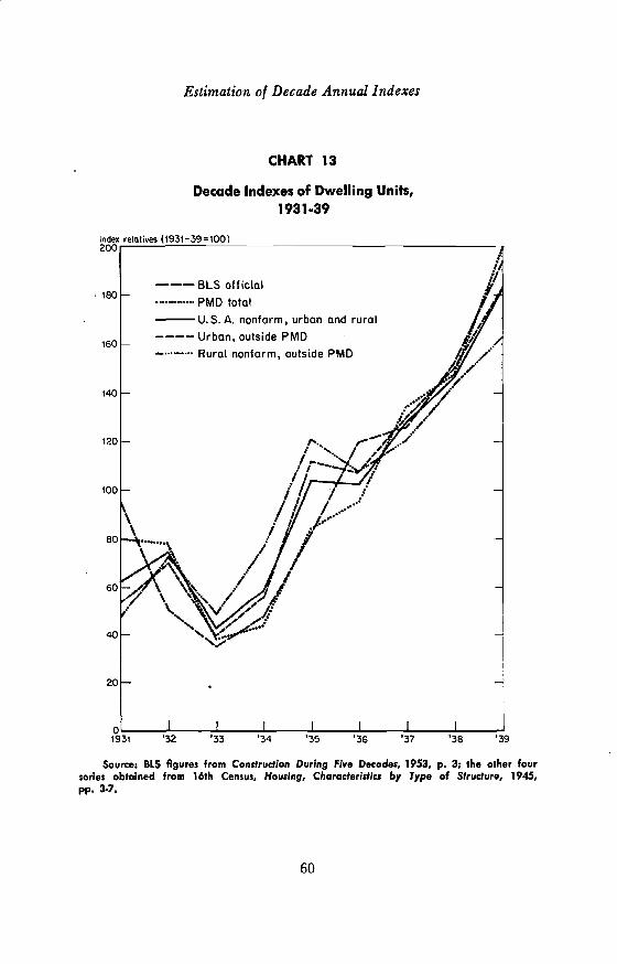
Estimation of Decade Annual Indexes
CHART 13
Decade Indexes of Dwelling Units,1931-39
Source: BLS figures from Construction During Five Decades, 1953, p. 3; the other fourseries obtained from 16th Census, Housing, Characteristics by Type of Structure, 1945,pp. 3-7.
60

Estimation of Decade Annual Indexes
TABLE 15
ESTIMATED PRODUCTION OF RESIDENTIAL HOUSEKEEPING UNITS,1840-1939
YearDecadeIndexes
HousingProduction Decade
(000) Year Indexes
Original HousingSeries Production(000) (000)
1840 69.01 36 1890 328 2781841 79.02 41 1891 298 2521842 65.45 34 1892 381 3231843 65.72 34 1893 267 2261844 73.32 38 1894 265 2251845 87.98 46 1895 309 2621846 111.16 58 1896 257 2181847 137.68 72 1897 292 247
1848 134.06 70 1898 262 2221849 157.71 82 1899 282 239
1850 78.28 94 1900 54.75 2301851 90.28 109 1901 78.58 3301852 100.70 121 1902 76.09 3201853 110.53 133 1903 82.65 3471854 114.72 138 1904 96.00 4031855 115.20 138 1905 127.42 5351856 112.13 135 1906 124.65 5241857 118.08 142 1907 112.26 4711858 86.09 103 1908 110.04 4621859 81.24 98 1909 137.22 576
1860 87.80 93 1910 113.13 4771861 71.32 76 1911 111.87 4721862 74.04 79 1912 120.93 5101863 69.35 74 1913 113.10 4771864 56.19 60 1914 110.73 4671865 76.62 81 1915 112.40 4741866 107.65 114 1916 110.58 4671867 131.86 140 1917 68.97 2911868 156.70 166 1918 40.14 1691869 159.06 169 1919 98.38 415
1870 118.63 158 1920 217 2501871 140.54 188 1921 491 491
1872 125.76 168 1922 767 7671873 130.39 174 1923 950 9501874 92.69 124 1924 963 9631875 95.53 127 1925 1,048 1,0481876 76.48 102 1926 1,010 1,0101877 77.11 103 1927 837 8371878 60.63 81 1928 741 7411879 67.16 90 1929 473 573
(continued)
61

Estimation of Decade Annual Indexes
TABLE 15 (concluded)
YearDecadeIndexes
HousingProduction
(000) YearDecadeIndexes
OriginalSeries P(000)
Housingroduction(000)
1880 48.76 127 1930 330 4851881 73.61 191 1931 254 3731882 80.19 208 1932 134 197
1883 91.43 237 1933 93 137
1884 94.89 246 1934 126 185
1885 102.73 267 1935 221 3251886 107.00 278 1936 319 4691887 125.61 326 1937 336 4941888 123.31 320 1938 406 597
1889 141.61 368 1939 515 757
NOTES
1840—59: Decade totals of 520,000 and 1,202,000 units distributed on the basisof decade indexes made up of the geometric average of Riggleman(Isard-adjusted) and Ohio building value. Ohio figures from unpub.lished tax increments (see discussion pp. 75 if.); Colean and Newcomb,Stabilizing Construction, p. 227.
1860—89: Decade totals of 1,061,000, 1,333,000, and 2,597,000 units for the
sixties, seventies, and eighties, respectively, were distributed by thegeometric average of the following indexes equally weighted: (1) Ohiostatewide, (2) Riggleman-Isard adjusted, deflated by a Riggleman costof building index, and (3) Long index-number residential buildingpermits (Long, Building Cycles, pp. 227-228; Colean and Newcornb,Stabilizing Construction, p. 226; Riggleman, Variations in BuildingActivity, pp. 257-258; Table 16 following).
1890—99: Blank's yearly estimates reduced by 15.3 per cent. Yearly totals inGrebler, Bjank, and Winnick, Capital Formation, p. 332, Table 15.
1900—19: Chawner's decade estimates of 4,200,000 and 4,220,000 distributed byindex relatives (1900-19=100) made up of simple average of Blank'sand Chawner's series (Blank, Volume of Residential Construction, p. 27,Table 13.
1920—29: Blank's new series at 7,497,000 for the decade (compared with officialseries at 7,034,000). Figures for 1920 adjusted by 33,000; figures for1929 raised by 100,000. The adjustment for 1929 was for "linkage"only and was for that reason arbitrary. The need for adjustmentindicates a hiatus in the sets of decade totals and yearly indexes.Ibid., p. 59.
1930—39: Official BLS-NBER yearly estimates (Construction During Five Decades,1953, p. 3), raised by 47 per Cent to make a 4,019,000 decade total.
Sum of indexes by decades differs from 1,000 because of use of geometric averagesand because of rounding. For the same reasons, production totals by decade also
differ slightly from the decade aggregates that were distributed.
62

Estimation of Decade Annual Indexes
raised them by a decadewide adjustment to offset the underestimationpreviously noted.
With Blank's decade total for the twenties, the decade index thatwent along with it was accepted.55 As Blank noted, this index correspondsclosely with that of the official series. I departed from his index for 1929to smooth the transition, and for 1920 because his estimate for that yearin the light of available information seemed unduly low.66
For the decades of the 1900's and 1910's, Chawner's decade totalswere used, as previously noted, but not the unmodified. index patternsthat went along with the totals. Blank's decade indexes involved decadetotals which, like Chawner's, were about the same in magnitude for thetwo decades though resting at a lower level. Blank's decade indexes reflecta more intensive working of a wider mass of empirical materials. Butsome of the pattern implicit in Blank's indexes must have been generatedby the underestimation of level running through them. Under the cir-cumstances it seemed reasonable to average the two sets of decade in-dexes. The average of the resulting pair of indexes is shown in Table
For the 1890's, Blank's index was used, since it was drawn from acity coverage much larger than other available indexes were. By 1890,his index is based upon 25 Cities accounting for 14.5 per cent of totalnonfarm population. In contrast, Long's residential permit index for1890 covered only 12 cities. The Riggleman index for 1890 has the requi-site coverage (32 cities) but it measures nonresidential as well as residen-tial building and it is cast in value terms. Only the Ohio residential build-ing index was suited for averaging with the Blank index. But since theBlank index was adjusted for nonurban building and since the two idexescorresponded closely (see Chart 14), the Blank index was accepted forthe nineties.58
For details see Blank, The Volume of Residential Construction, p. 59.56 Estimates for the year 1920 compare as follows: Wickens (1941), 247;
Chawner (1939), 300; Blank (1954), 217; BLS (1959), 247. (Blank, Volumeof Residential Construction, Table 13, p. 59; Wickens, Residential Real Estate,p. 49; Chawner, Residential Building, p. 13; Construction During Five Decades,p. 3.)
57 See the detailed discussion of the Chawner and Blank indexes in Blank,Volume of Residential Construction, pp. 25-28.
58 With the index relative, 1890-99 = 100, the combined decade indexes areas follows for the years beginning 1890:
1890 1891 1892 1893 1894Blank, alone 115.6 101.4 129.6 90.8 90.1Blank-Ohio average 102.7 109.6 127.6 100.7 89.3
1895 1896 1897 1898 1899Blank, alone 105.1 87.4 99.3 89.1 95.9Blank-Ohio average 102.7 89.0 93.5 87.6 99.4
63

Estimation of Decade Annual indexes
For the three decades between 1860 and 1890, difficulty was experi-enced in devising appropriate annual indexes. None of the standardavailable measures had a claim to special validity in those three decades.Blank's index was too limited in coverage to be used alone for the 1880's.The Ohio experience is likewise unsuitable as a sole measure of nation-wide patterns of movement, since Ohio overresponded to the rise of thesixties and underresponded to the boom of the eighties. The annualstatewide Ohio returns for residential production also include farm dwell-ings, which played a variable role over those three decades. Newly erectedfarm dwellings are estimated to account for 27, 50, and 13 per cent ofaggregate decade production of houses during the l860's, 18 70's, and1880's, respectively (see Table ii, columns 1 and 6). There is no reliableway to remove the influence of farm construction from annual aggregatestatewide returns. Aggregation of returns separately for highly urbanized
64
CHART 14
Decade Indexes for the 1890's
1890 '91 92 '93 '94 '95 '96 '97 '98 '99
Source: Grebler, Blank, and Winnick, Capitol Formation, p. 332; unpublished Ohioyearly totals.
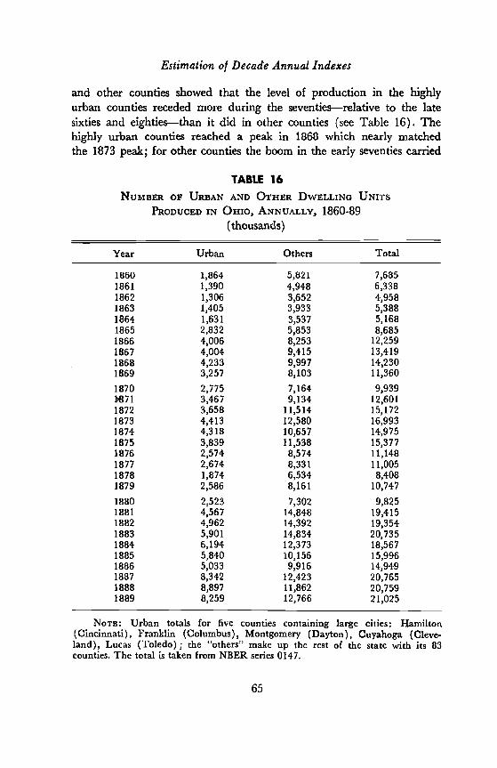
Estimation of Decade Annual Indexes
and other counties showed that the level of production in the highlyurban counties receded more during the seventies—relative to the latesixties and eighties—than it did in other counties (see Table 16). Thehighly urban counties reached a peak in 1868 which nearly matchedthe 1873 peak; for other counties the boom in the early seventies carried
TABLE 16
NUMBER OF URBAN AND OTHER DWELLING UNITSPRODUCED IN OHIO, ANNUALLY, 1860-89
(thousands)
Year Urban Others Total
1860 1,864 5,821 7,6851861 1,390 4,948 6,3381862 1,306 3,652 4,9581863 1,405 3,933 5,3881864 1,631 3,537 5,1681865 2,832 5,853 8,6851866 4,006 8,253 12,2591867 4,004 9,415 13,4191868 4,233 9,997 14,2301869 3,257 8,103 11,360
1870 2,775 7,164 9,9391'871 3,467 9,134 12,6011872 3,658 11,514 15,1721873 4,413 12,580 16,9931874 4,318 10,657 14,9751875 3,839 11,538 15,3771876 2,574 8,574 11,1481877 2,674 8,331 11,0051878 1,874 6,534 8,4081879 2,586 8,161 10,747
1880 2,523 7,302 9,8251881 4,567 14,848 19,4151882 4,962 14,392 19,3541883 5,901 14,834 20,7351884 6,194 12,373 18,5671885 5,840 10,156 15,9961886 5,033 9,916 14,9491887 8,342 12,423 20,7651888 8,897 11,862 20,7591889 8,259 12,766 21,025
NOTE: Urban totals for five counties containing large cities: Hamilton(Cincinnati), Franklin (Columbus), Montgomery (Dayton), Cuyahoga (Cleve-land), Lucas (Toledo); the "others" make up the rest of the state with its 83counties. The total is taken from NBER series 0147.
65

Estimation of Decade Annual indexes
residential building to levels nearly a third above the peak of 1868. Onthe other hand, the long-swing contraction was equally marked in bothcategories; and total specific amplitude of residential building tends tovary, if at all, inversely with degree of urbanization.59 Thus while ourtotal statewide building index is serviceable, possible merit may be foundin separate use of its highly urbanized and other components.
The Long index before 1890 reflects the building experience of afew metropolitan centers. It is excessively weighted with New York(Manhattan) experience and fails to allow adequately for secular growth.The Riggleman index as adjusted by Isard is also metropolitan in char-acter but during those decades it is much more broadly based and lessdependent upon eastern seaboard building patterns. The index measuresthe value of total urban building, not of residential units; and smalltowns and cities are not adequately weighted in the index. Besides thesemajor indexes, we have available separate city returns for Manhattanfrom 1868 and for Chicago from 1860 on.
Two possible approaches were explored in detail. First, an effortwas made to assess index availabilities for each decade and to select anappropriate set of indexes with changing weights. The judgment in-volved in selecting components and assigning weights was inherentlyopportunistic and marked by some arbitrariness, but variation of weightsand components by decades improved judgment for each decade. Thethree sets of decade indexes developed in this fashion are shown in thenext tabulation.6°
59 Below are urbanization indexes, chronologies, and specific amplitudes forstatewide Ohio and its sample groups.
Amplitude Urban Population Farm Mortgages a-sSam pie Specific Cycle as Per Cent of Per Cent of TotalGroup Peak Trough Fall Total, 1920 Value, 1885
I 1874 1878 85.2 93 12II 1868 1878 86.7 83 39III 1868 1878 83.4 77 37IV 1872 1878 102.5 43 57V 1875 1878 118.7 20 84
State 1873 1878 74.5 64 49°°For the decade of the eighties Blank's index was combined with the Ohio
statewide index, with Long's index of residential permits, and with Riggleman'sper capita building permits (see Chart 15 and Table 17). An alternative averageof a set of indexes including Chicago and Manhattan corresponded in patternwith the simple average of the four indexes. The high amplitudes of the Longindex should offset the limited downward bias in the population adjustmentof the Riggleman index. For the decade of the seventies, a broadly based Blankindex was no longer available, and greater reliance had to be placed on theRiggleman index with its broad coverage. It was assigned a double weighting.The Riggleman deflated index was used, since in the decade a profound price
66

Estimation of Decade Annual Indexes
Component Weight Allowed in Decade IndexActwztzes 1860 s 1870 s 1880 s
Ohio, statewide 1
Rigglemari, per capita 1
Riggleman, per capita deflated 1 2
Blank, residential units 1
Long, number residential permits 1 1 1
Ohio, urban I 1
Ohio, other 1 1
Tables 17-19 and Charts 15-17 show the behavior of the severalindexes and their averages. Application of the averages to our decadetotals yielded a set of annual building totals, reproduced in Chart 18,"shifting weight variant." The second procedure used to derive decadeindexes for 1860-89 involved a constant set of series with unchangingweights for the three decades. This eliminated the arbitrariness involvedin shifting indexes and weights by decades though it entails a less efficientuse of available information. The most serviceable index measures run-ning for the three decades were found to be Ohio, statewide; Long,number of residential permits; and Riggleman-Isard, deflated value ofbuilding permits. It was necessary to deflate the Riggleman-Isard seriessince in the period covered a profound price revolution distorted valuecalculations cast in current prices. The three series reflect, in differentways and with different degrees of emphasis, divergent tendencies ofUnited States building experience. Fortunately, the main outlines ofmovement being shared, the pattern of weighting was not too difficult.In the absence of measured criteria, each index was weighted equally andaveraged geometrically. As Chart 18 shows, the constant weight andvariable weight series conform closely, facilitating selection of the con-stant weight series because of the simplicity of its design.
revolution distorted value calculations cast in current prices. It was felt thatthe upward bias in a metropolitan building series and inclusion of Long's high.amplitude and limited-coverage index offset the downward bias inherent in theper capita adjustment. Since the Riggleman index in the seventies did not coverOhio cities, separate averaging of the Ohio urban index, with its five large urbancounties, was deemed justifiable. The Ohio nonurban index was included to repre-sent smaller urban patterns of movement. A test computation of another plausiblepair—Riggleman and Ohio nonurban—displayed a parallel pattern. The broaderbased average was selected (for indexes, see Table 18 and Chart 16). For thedecade of the sixties, the combination of Riggleman, Long, and Ohio urban andnonurban was used. Because of its reduced coverage of only six cities (four east-ern seaboard, plus Milwaukee and Indianapolis) and its predominant reflectionof eastern seaboard urban experience, the Riggleman index was weighted onlyonce. While inclusion of two Ohio indexes may not be fully defensible, bothreflect patterns of economic activity running through the whole central north-west territory. In the absence of better information, their inclusion seemed justi-fiable (see Table 19 and Chart 17).
67
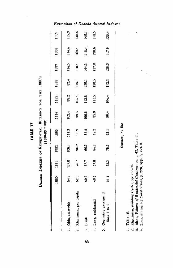
TA
BLE
17
IND
EX
ES
OF
RE
SID
EN
TIA
L B
UIL
DIN
G F
OR
TH
E 1
880'
s10
0)
SOU
RC
E, b
y lin
e
1.T
able
16.
2.R
iggl
eman
, Bui
ldin
g C
ycle
s, p
p. 2
58-6
0.3.
Bla
nk, V
olum
e of
Res
iden
tial C
onst
ruct
ion,
p. 4
2, T
able
11.
4.L
ong,
Sta
biliz
ing
Con
stru
ctio
n, p
. 228
, App
. B, s
ect.
3.
03
1880
1881
1882
1883
1884
1885
1886
1887
1888
1889
1.
Ohio, statewide
54.2
107.0
106.
711
4.3
102.
488
.282
.411
4.5
114.
4115.9
2.
Riggleman, per capita
62.3
76.7
90.9
98.9
93.3
104.4
115.1
118.4
109.4
130.6
3.
Blank
50.8
57.7
60.5
83.8
100.6
113.8
130.1
144.3
118.4
140.1
4.
Long, residential
40.7
57.8
64.2
79.2
89.9
113.5
128.5
137.0
130.6
158.5
5.Geometric average of
lines
1 to
451
.472
.378
.393
.196
.410
4.4
112.
212
8.0
117.
913
5.4
0 -I'
C.'

TA
BLE
18
DE
CA
DE
IND
EX
ES
OF
RE
SID
EN
TIA
L B
UIL
DIN
G F
OR
TH
E 1
870'
s
1870
1871
1872
1873
1874
1875
1876
1877
1878
1879
1.R
iggl
eman
per
mits
per
cap
ita,
(191
3 do
llars
)13
8.9
147.
911
5.3
111.
895
.696
.479
.973
.964
.875
.5
2.L
ong,
res
iden
tial,
num
ber
of p
erm
its (
1870
-79=
100)
139.
116
9.6
126.
112
6.1
89.1
89.1
73.9
80.4
56.5
50.0
•
3.O
hio,
num
ber
of u
rban
resi
dent
ial (
1870
-79=
100)
86.2
107.
711
3.7
137.
113
4.2
119.
380
.083
.158
.280
.4
4.O
hio,
num
ber
of n
onur
ban
resi
dent
ial (
1870
-79=
100)
76.1
97.0
122.
213
3.6
113.
112
2.5
91.0
88.5
69.4
86.6
5.G
eom
etri
c av
erag
e,lin
es 1
to4
111.
913
1.1
118.
412
3.6
104.
310
3.9
80.8
79.8
62.6
72.4
SouR
cE: S
ame
as f
or T
able
17.
0 0

-4
TA
BLE
19
DE
CA
DE
IND
EX
ES
OF
RE
SID
EN
TIA
L B
UIL
DIN
G F
OR
TH
E 1
860'
s
SOU
RC
E: S
ame
as f
or T
able
17.
0
1860
1861
1862
1863
1884
1865
1866
1867
1868
1869
1.R
iggl
eman
, per
mits
per
capi
ta (
1913
dol
lars
)12
6.0
83.2
72.4
87.1
52.1
74.9
101.
711
8.0
136.
614
7.8
2. 3.
Lon
g, r
esid
entia
l, nu
mbe
rof
per
mits
(18
60-6
9=10
0)
Ohi
o, n
umbe
r of
urb
anre
side
ntia
l (18
60.6
910
0)
85.7
71.9
62.9
53.6
91.4
50.4
88.6
54.2
45.7
62.9
62.9
109.
2
88.6
154.
5
125.
7
154.
4
160.
0
163.
3
188.
6
125.
6
4.O
hio,
res
t of
stat
e,-
num
ber
of r
esid
entia
l(1
860-
6910
0)91
.777
.957
.561
.955
.792
.212
9.9
148.
215
7.4
127.
6
5.G
eom
etri
c av
erag
elin
es1
to 4
91.9
68.4
66.2
71.3
53.7
83.0
116.
013
5.7
154.
014
5.4

Estimation of Decade Annual Indexes
CHART 15
Decade Indexes of Urban Building for the 1880's
Source: Table 17.
71
reicitives t1880—89100)
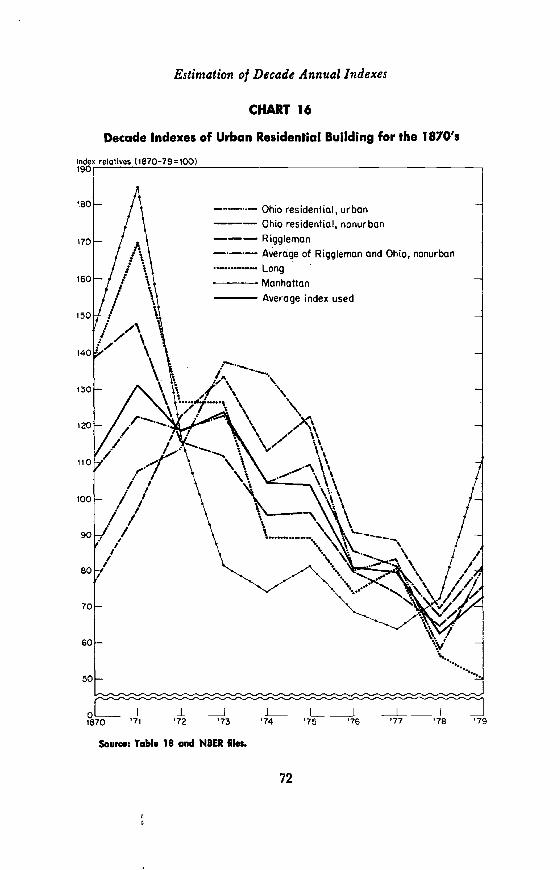
Estimation of Decade Annual Indexes
CHART 16
Decade Indexes of Urban Building for the 1870's
72
$ourcoi Table 18 and NBER files.

Estimation of Decade Annual Indexes
CHART 17
Decade Indexes of Urban Residential Building for the 1860's
73
63
Source: Table 19 and NBER files.

Estimation of Decade Annual Indexes
CHART 18
Estimated Annual Residential Production,Constant and Shifting Weight Variants,
1860-89
Source: Constant weight: Table 15, years 1860-1889. Shifting weight: Tables 17, 1819, geometric average, multiplied against decade totals listed in notes to Table 15.
74

Estimation of Decade Annual Indexes
In applying annual indexes to the decade total for the 1860's allow-ance was made for replacement of Civil War losses in housing. Of the esti-mated 1860 stock of nonfarm dwellings, an estimated 22 per cent or628,000 were in the South. Civil War damage was intense in certainareas: the upper valley of the Shenandoah; the country between Wash-ington, D.C. and Richmond; cities such as Atlanta, Columbia, Nashville,Charleston; the belt of territory ravaged by Sherman's army; and otherareas of concentrated fighting.01 By a rough guess on the basis of estima-tion of the populations involved, housing production for 1866-69 wasraised 'by 32,000 units (see Table 15 and notes).
We turn now to the estimation of the annual series for 1840-59.The only comprehensive annual indexes of building available are thosederived from Ohio and the Riggleman study. The Riggleman index forthose decades reflects building rates in the eastern seaboard urban com-munities of Manhattan, Boston, and Washington. (Three other citieswere added to the index, but either late in the surveyed years or withlittle effect on the totals.) The Ohio index for the two decades wasderived from the 1840-60 record of increments of real property assess-ments in Ohio municipalities converted into building value with the aidof regression analysis of total value of new building and annual incre-ments of the assessed value of municipal (town, village, and city) realproperty between 1858 and 1889. The regression involved problems oftwo separate classes. There was, first, the need to adjust the correlatedvariables for comparability and, second, to design an adequate regressionrelationship which "fitted" the observed relationship.
The total value of building as initially reported in Ohio buildingstatistics, including farm and nontaxable public building, was utilized as
61 Sherman's march through Georgia and the Carolinas allegedly was accom-panied by much burning and destruction, "not a building [was left] on the railwayfrom Macon to Savannah" (0. Eisenschiinl and R. Newman, The Civil War,New York, Grosset & Dunlap, Vol. I, 1956, p. 658; E. M. Coulter, The SouthDuring Reconstruction 186.5-1877, Baton Rouge, Louisiana State University Press,1947, p. 1). The upper valley of the Shenandoah, according to J. B. McMasters,"was a scene of desolation. . . . Beyond Harrisonburg, toward Staunton, was theregion laid waste by Sheridan, and there, within a circle five miles in diameter,scarcely a house, barn, mill or building of any sort was standing." The countrybetween Richmond and Washington was "like a desert." Homes of Union volun-teers in Tennessee and northern Georgia "had been ruined by rebel armies orguerillas." Charleston was allegedly a city of "ruins" (A History of the Peopleof the United States During Lincoln's Administration, New York, D. Appleton,1927, pp. 637-640). Columbia, S. C., was burned under official orders. A tentativenumber of 32,000 dwelling units was allowed for war loss. According to generalhistorical accounts rebuilding was speedy (see Coulter, op. cit., p. 255 if.). Hencethe war replacement was spread over 1866-69 and moderately peaked in 1866.
75

Estimation of Decade Annual Indexes
one of the correlated variables. Property-tax assessment reports refer tononfarm real property, excluding public or quasi-public property. Despitethese elements of noncomparability, the levels of building and tax-assess-ment increments, as shown in Chart 19, were closely aligned throughoutthe entire period. The nonfarm taxable building predominated in totalbuilding values, even in the early period of the comparison; and possiblythe relative movement of farm and public building was mutually off-setting. At a later stage of the research, another regression was preparedbetween assessment increments and building values, fully adjusted forcomparability. The assessment increments were for all real property (farmand nonfarm) and the taxable building excluded all public and quasi-public building (which would not be represented in the assessments).The fit during the "regression" period is somewhat closer in the secondcase.°2 These more closely matched variables apply to all building andproperty increments and, in the early years 1837-55, the changes in farmreal estate assessment dominate the assessment totals. The relative shareof nonfarm assessments was rising rapidly during those years. Since thepresent quest is for a nonfarm building index, it seemed desirable toutilize the regression which applied only to assessment increments in mu-nicipal property.
The assessment increments measure the net resultant of the assessedvalue of (1) old buildings dropped from the tax rolls because of demoli-tion or destruction, (2) assessed values of newly erected structures orimprovements added to the tax rolls, and (3) revaluations of propertiesalready on the rolls. Revaluations disturb the relationship between netnew building and net change in assessments. Before 1846, the disturbanceswere marked owing to laxity in assessment and weak central supervision.After 1846, disturbances due to revaluations were scaled down, since re-valuations were concentrated in scheduled reappraisal years set at firstfor 1853 and 1859, thereafter, decennially. The upward shift of valuesresulting from revaluations was sizable in 1853 and in 1870. Assessed val-ues for identical or nearly identical properties were raised 61 per cent and60.9 per cent, respectively, reflecting the inflations of 1846-53 and 1861-66. The revaluation of 1859 showed a 5.5 per cent fall in the level ofreal estate values fixed in 1853. After 1870, the standard of assessmentseemed fixed and resulted in a widening gap between assessed and marketvalues. Outside the reappraisal years, revaluations were permitted only
62 See charts of these matched variables and description of regression in mypaper, "Value of Nonfarm Building, Residential and Nonresidential, U.S.A.,Annually, 1850-1939," submitted to the Conference on Research in Income andWealth, Chapel Hill, North Carolina, September 4-5, 1963.
76

Estimation of Decade Annual Indexes
Million dolicirs
CHART 19Ohio Building, 840-89
77
1840 '45
Source: Assessments from state auditor's annual reports, as reported by letter fromauditors' offices, and as compiled for this study by the Secretary of the State of Ohio.Value of new building was extracted from annual reports of the Secretary of State. Thesedata are unadjusted for assessment undervaluation.

Estimation of Decade Annual Indexes
in exceptional circumstances and appear to have affected only smallfractions of assessed property on the rolls.68 Disturbances thus introducedinto the relationship between building and assessment increments couldbe offset or neutralized by smoothing with a 3-year moving average.
The level of assessment or relationship of assessment values to marketvalues was, for years after 1846, accepted as originally prepared for taxuse. The first three major reappraisals—1846, 1853, and 1859—resultedin a level of assessments which closely approximated market value.04
The level of assessment gradually receded after the Civil War andby 1890 hardly covered more than two-thirds of the value of the prop-
Since, however, recorded values for new building reflected valuesestablished for tax assessment, correction of both tax-assessment and build-ing value statistics was not required. On the contrary, for the few yearsbefore 1846, when properties were evaluated for tax purposes at one-fourth to one-third of market value,60 use of those values as a base forregression projection would have understated building in the early forties.Hence, for years before 1846, assessment values were doubled.°7
6.3 Revaluations were carried out periodically at intervals of 6 to 10 years.Pending reappraisal, old properties were assessed at fixed values. Hence, incrementsin assessed value, as noted in an official report, were "principally occasioned bynew structures" (Annual Report, State Auditor, Ohio, 1865, P. 22). In the 1866report it was noted that "real estate stands taxed on the value fixed upon itin 1859" (ibid., 1866, p. 20).
64 The census estimates of true value of all taxable property (real and per.sonal) for 1850 and 1860 were understated by 19.6 and 14.0 per cent, respec-tively. In the contemporary view of the Ohio statistics commissioner, understate-ment was concentrated in personal property (see Ohio Statistics Commissioner,Sixth Annual Report, 1862, P. 24). His finding was confirmed by deed surveysfor the periods Apr.—Oct. 1853 and the year ending 1859, showing that assess-ment of sold properties ran to 87.4 and 101.0 per Cent of market value (Proceed-ings 1853, Board of Equalization, Columbus, Ohio, 1854; Ohio Executive Docu-ments, 1859, part I, PP. 857-860).
See data and reports collected in my paper, "Value of Nonfarm Build-ing."
66 One responsible judgment was that, before 1846, assessed values ran to aquarter of market values (E. L. Bogart, Financial History of Ohio, University ofIllinois Studies, 1912, p. 210). The 1846 reassessment boosted the values ofassessed urban property by 256 per cent. The Ohio statistics commissioner notedthat "prior to 1846 the assessments fall so much below the real values that theyafforded but little criterion of the actual wealth" (bc. cit.). On the 1846 revamp-ing, see the history and appraisal in Bogart, Financial History of Ohio; and ThePassing of the Frontier, 1825-1850, C. Wittke, ed., Columbus, Ohio State Archeo-logical and Historical Society, 1941, pp. 425-430.
67 Actual annual assessment increments for real property located withinmunicipal corporations, the increments adjusted for undervaluation before 1846,
78

Estimation of Decade Annual Indexes
The form of the regression presented difficulties. A trial estimationwas made by fitting a linear regression line between new-building and tax-assessment increments. The results showed a systematic bias in the es-timated value; on the expansion phase, there was a tendency towardoverestimation and, on the contraction phase, underestimation reflectinga tendency for assessment revaluation of old properties to exaggerateswings. An attempt to allow for this behavior by using a multiple-linearregression function, including annual percentage change as a variable,did not produce workable results. The coefficient of correlation was .69.After tests of several other multiple-regression linear functions, also withunsatisfactory results, the correlation formula finally employed was anaverage of two simple linear functions, with and without constant terms,fitted separately to expansion and contraction phases. The coefficient ofcorrelation of the resultant composite function is .94. The estimatedvalue for new building from 1840 to 1857, along with actual values from1858 on and smoothed assessment increments from 1840 on, are presentedin Chart 19. Since the bases for regression are assessment increments inmunicipal real property, our projected values for new building reflectprimarily nonf arm activity. The previously mentioned regression, basedon increments of all real property including farms, involves a later troughfor nonfarm activity in 1844 as against 1840, and a much dampenedrise during the forties.
As indicated, neither the Riggleman nor the Ohio indexes are on asstrong a footing for the decades before 1860 as for the decades following.In addition, they pertain to the total value of metropolitan and urban
and our three-year moving averages appear below. Since 1841 was a reappraisalyear, the high negative value recorded for that year and the sizable gain for thesubsequent year reflect the vagaries of shifting appraisal policy. For the calcula-tions, the year 1841 was treated as zero.
Actual Adjusted 3-Year MovingAnnual Annual Average
(dollars in thousands)1839 441.3 882.6 —1840 308.0 616.0 4991841 —510.3 0 7911842 878.3 1,756.6 6671843 122.4 244.8 1,041
1844 561.5 1,123.0 1,051
1845 1,788.2 1,788,2 1,5371846 n.a. 1,700.0 1,7031847 1,620.1 1,620.1 1,8731848 2,298.3 2,298.3 1,958
79
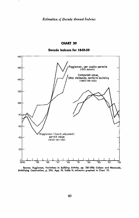
Estimation of Decade Annual Indexes
CHART 20
Sources Riggleman, Variations in Building Activity, pp. 287-288; Colean and Newcomb,Stabiflxing Construction, p. 226, App. N, Table 2; estimates graphed in Chart 19.
80
Decade Indexes for 1840.59

Estimation of Decade Annual Indexes
building, which shares the swings of residential building, but often withvariations in timing and amplitude. The amplitude and upward driftof the Riggleman index, as adjusted by Isard and used here, fit moreclosely to our accepted decade estimates of nonf arm residential building.Neither the Ohio nor the Riggleman series is deflated, partly becausevalue shiftings in the period were difficult to measure accurately andpartly because of doubt that Ohio assessments were adjusted to shifts incurrent costs. The resulting average of the two sets of decade indexes—Ohio nonfarm and Riggleman (isard adjusted)—can lay out only thegeneral course of residential building within those decades.
The two sets of decade indexes, along with Riggleman per capita per-mits in 1913 dollars, are shown in Chart 20. Since the movement is acommon one, a geometric average (detailed in Table 15) of the twoselected indexes was computed for use in projecting nationwide nonfarmresidential building. An interesting check on the order of magnitude ofour estimates for 1840-60 is afforded by the ratio of the 1857-59 recordedOhio count of dwelling production to estimated nationwide dwellings.The Ohio share for 1857-59 is 6.3 per cent compared with 8.0 per centfor the decade of the sixties. The acceleration in Ohio building relativeto nationwide levels was also found to characterize urban growth rates inOhio and the nation (Chart 8). Another test for order of magnitudeshows that residential building in 1844 in four large cities, accounting for16.8 per cent of total estimated 1840 nonfarm population, amounted to18.3 per cent of our nationwide nonfarm estimate for that year.°8 Ourorder of magnitude holds at least for this segment of the period.
The editor of the Cincinnati Miscellany (Vol. II, 1864, p. 58) compiledthe number of houses built in 1844 in Philadelphia, Boston, New York City, andCincinnati (6,422). This is 18.3 per cent of our nationwide estimate for thatyear. The four Cities had a census population in 1840 of 939,597. We estimatenonfarm population by scaling down our 1860 estimate (see footnote 39) in theratio of the movement of nonagricultural labor force between 1840-60. Thusderived, the estimated nonfarm population in 1840 was 5.61 million of which ourfour-city share was 16.75 per cent.
81

6
Evaluation of Total Series
Despite their patchwork makeup by a combination of separately fashioneddecade totals, the ten resulting sets of annual estimates of residentialbuilding fit together with little need for smoothing. Only one decadeending, that of 1929, was altered to smooth the connection. The re-sulting series is set forth in Table 15 and shown in Chart 21, togetherwith the Long, Riggleman (Isard adjusted), and the Blank series.
All the major movements which run through these indexes, includingshort cyclical play, are reflected in ours. The new index is believed tocatch more accurately the true secular drift and the relative play of longswings. The following tabulation of average long-swing amplitude andsecular growth rate shows that the new index, compared with othermeasures, has low amplitude but relatively high secular growth. Fivefeatures of the new series call for detailed comment.
Number Total Long-termof Average Rate of Growth
Years Long Specific (percentSeries Covered Cycles Amplitude per annum)
Riggleman-Isardindex buildingpermits 1862-1933 4 230.0 4.03
Gottlieb 1862-1939 4 200.4 2.74Long index number
residential permits 1856-1936 4 278.6 l.59a
Blank new dwellingunits started 1889-1959 4 249.1 1.90
Growth rate for Long's index of the total number of permits. (M. Abramo-vitz, "Evidences of Long Swings in Aggregate Construction Since the Civil War,"a National Bureau study, in preparation, Tables 7, 16).
First, the series shows a double peak between 1868 and 1871 with asizable fall between, regarded here as corresponding with the nature ofthe post-Civil War expansion. The expansion in Ohio, where its coursemay be clearly traced, ebbed and flowed in course. As Table 16 and
82
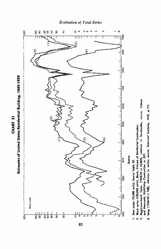
CH
AR
T 2
1
Est
imat
es o
f Uni
ted
Sta
tes
Res
iden
tial B
uild
ing,
184
0-19
39
e,.. 0 -q
cJ3
Sou
rce
I. N
ew s
erie
s (1
0,00
0 un
its),
Sou
rce
Tab
le 1
5.2.
Ski
nk s
erie
s (1
00,0
00 u
nits
), B
lank
, Vol
ume
of R
esid
entia
l Con
stru
ctio
n.3.
Rig
glem
an-I
sard
inde
x(1
920-
29 =
10,
000)
,re
lativ
esin
hund
redt
hs,
sour
ce,
Col
ean
and
New
com
b, S
tabi
lizin
gC
onsf
rucf
ion,
p. 2
27.
4.Lo
ng (
1920
.30
100)
, rel
ativ
es in
tent
hs, s
ourc
e, H
isto
rical
Sta
tistic
s,19
49, p
.173
.

Evaluation of Total Series
Chart 22 show, the 1868-69 peak was sizable and the resulting ebb wasalmost as serious as the decline after 1873-74. Ohio marriages show apeak in 1866, while the national marriage rate was higher in 1867 thanin later years.°9 Both data indicate an ebbing in household formationbetween 1867 and 1871. If our decade patterns are right, then the earlypost-Civil War peak rivalled that of the early seventies.
Second, the housing decline of the seventies and boom of the eightiesare moderate in amplitude. The relative conformation of housing pro-duction in the two decades is no quirk of a statistical mosaic but reflectsthe tendency for realized amplitudes to dampen as a wider range ofurban-size classes and regions is covered by the aggregate.
Third, the new index shows a substantial decline in the ninetiesrelative to the boom of the 1880's and 1900's, a pattern of movementshared by both the Riggleman (Isard) and Long series.
Fourth, in our series the sharp drop of 1900, which characterizespermit-derived series (Riggleman, Long, Newman, Blank), is greatly
reduced. Since the sharp drop sets a long-swing trough it merits detailedenquiry. The relative behavior of the various permit-derived series is set
•• forth in a note below.70 The mild drop in the Chicago building permit
09 Ohio and national marriage data are as follows:Ohio
Number ofYear Marriagesu
1858 21,3521863 19,187
• 1865 22,4041866 30,5791867 29,2301868 27,7981869 25,625
• 1870 25,4591871 24,8491872 26,616
• 1873 26,692SouRcE: files; Historical
Series C77.Year ending June 30.
70 Some of the permit-derived series for 1899-190 1 follow:• 1899 1900
Riggleman, per capita permits ($) 31.37 21.71• Chicago, building permits value ($ mill.) 20.9 19.1
Long, index, residence permits(1920-30=100)
Blank, number dwelling units (000's)
Ohio Statistics, NBER
NationMarriagesper 1,000
9.69.08.98.88.89.09.0
1949, p. 44,
190130.5934.9
Statistics,
38 28 36282 189 275
84

Evaluation of Total Series
CHART 22
Number of New Dwellings, Ohio, 1857-1914
Source: NBER files of Ohio building data.
1899 1900 1901
Newman, building index (1913=100) 70 46 66Number of dwelling units
BostonBrooklynManhattan
3,700 2,378 2,5699,966 5,939 7,012
29,447 8,996 19,7451,278 1,323 1,620
222 323 6291,390 1,287 1,850
DetroitSan AntonioSt. Louis
SOURCE: M. Colean, American Housing, NY, 20th Century Fund, 1949,p. 408; GBW, p. 332; Riggleman, Variations in Building, pp. 260-1; Long,Building Cycles, App. B., p. 228; Newman, Building Industry, p. 63, Table IX,coL 4.
85

Evaluation of Total Series
series is inexplicable in view of the famous strike which paralyzed buildingin that city during most of The report of building in Ohio showsa mild drop, while the nationwide production of 'building materials andthe behavior of building prices testify, not to a drop in 1900, but to arise.72 Many cross-checking measures of building trade unemployment failto indicate deterioration in General building trade reports indicate
71 Though Hoyt omits mention of the strike, it was well publicized in thebuilding trade and made national news. A general contractor lockout in the build-ing trades, instituted Feb. 5, 1900, paralyzed Chicago building until May 1901(R. B. Montgomery, Industrial Relations in the Chicago Building Trades, Chicago,University of Chicago Press, 1927, pp. 28 ff.). For current notice see the buildingtrade journal, Carpentry and Building, Jan. (editorial), Aug., Sept., and Nov.1900. See also detailed hearings before the Industrial Commission (Report of theIndustrial Commission on the Chicago Labor Dispute of 1900, Commission Report,Vol. 8, 1900).
See the following record of behavior (values in dollars)Building
Ohio, Value Shaw Deflated MaterialTotal Ohio, Number Construction Prices
Building Dwellings Material (BLS index)1898 24,327 15,237 1,341,569 39.61899 29,412 18,237 1,246,964 43.61900 29,748 15,967 1,425,045 46.21901 41,102 22,796 1,618,673 44,3
Source: NBER file 0147; unpublished adjusted building value; HistoricalStatistics, 1949, Series H50, p. 171, Series L22, p. 234. The 1900 Census editors'report on clay products manufacture noted that the census report for the yearending May 31, 1900, showed that the building trades were not yet "fullyrecovered from the panic of 1893" (1900 Census of Manufactures, p. 904). Aspecial census report comparing manufacturing activity in the census year withthe preceding year (1898-99) showed that brick and tile output in the censusyear was 16 per cent above that in 1898-99 (ibid., p. lxi).
See Paul Douglas, Real Wages in the United States, 1890-1926, Boston,Houghton Muffin, 1930, pp. 135-6.
Union Wage Rates, AverageBuilding Trades Workweek
(cents) (hours)1898 34.8 49.51899 36.1 48.91900 37.4 48.31901 39.1 47.5
In New York and Massachusetts, unemployment rates for 1900 showed a moderatepercentage rise (though the peak was 1897): 1897, 32; 1898, 28.3; 1899, 20.9;1900, 26.7; 1901, 17,8 (Douglas and A. Director, The Problem of Unemployment,New York, Macmillan, 1931). More conclusive on building trade unemploymentin 1900 is a census count of unemployment for the year ending May 31, 1900.It showed, when compared with a similar count in 1890, higher percentage ratesof unemployment during the same portion of the census year:
86

Evaluation of Total Series
marked slacks in Boston, Manhattan, and. Chicago and a varied pictureelsewhere, but no state of general decline.74 Real estate indexes of market
1899-1900 1889-90Carpenters and joiners 41.4 31.8Masons 55.5 42.9Painters, etc. . 42.4 31.1
As the census editor noted, the results are not comparable because of loose fram-ing of the census questionnaire and failure to make allowance for normal seasonalunemployment or work interruptions due to weather, etc. Even in the moreprosperous year that followed, 1901, a survey of annual earnings showed the widedistribution of full days worked by building trade workers (assuming a wage of37.5 cents per hour, a fifty-hour week, and the average layoffs):
Average Estimate, Per Cent Full .Days WorkedNumber Days Worked 230 Bricklayers 1,095 Carpenters
27 0.4 0.540 0.4 0.967 1.3 2.593 7.4 6.3
120 8.3 12.1147 8.7 18.2173 19.1 23.5200 25.6 22.4227 20.9 7.1253 11.7 4.7293 1.9
(see Cost of Living and Retail Prices of Food, Department of Labor, p. 280 if.).Reworking the 1889 and 1899 census results to allow for "normal" building tradeunemployment, Douglas and Director (p. 30) found the percentages of unemploy-ment were 8.8 per cent in 1889-90 and 12.8 per cent in 1899-1900, about whatwould be expected without a sharp drop in residential building in 1900.
A "great and . . . general" falling off of building work was reported forNew York City (Carpentry and Building, July 1900, p. 195), but it was ascribedto resistance to sharp 25 per cent increases in building material prices—charac-teristic of cyclical peaks. The monthly reports, "What Builders are Doing," for1899 and 1900, reflect an uneven but not a dull picture for 1900.
Baltimore, "quiet though about normal," Aug.; Boston, off '99 by 30 percent, July, but suburbs strong, Nov.; Cleveland, off '99 by 7 per cent; Columbus,Ohio, "very encouraging," up 25 per cent over '99, Nov.; Denver, "gratifyingincrease" over last year, Nov.; General Report, "it is well known that buildingoperations have been on a comparatively small scale all over the country," Nov.;Hartford, Conn., "building quite active just at present," Nov.; Kansas City, Mo.,"considerable amount of work in progress, . . . greater than at any time during thepast ten years," Nov.; Los Angeles, "year expected to far exceed 1899," Aug.;Manhattan, off '99, 25 per cent, July; Memphis, Tenn., 27 per cent over 1899,Nov.; Milwaukee, off '99 by 35 per cent, July; New Haven, Conn., "showing moreactivity in building operations," July; New Orleans, "greater than ever before,"Nov. and Dec.; Omaha, busier in July than in "a series of years," July; PiUs-burgh, "new record," 33 per cent over '99, July; Portland, Maine,
. "building
87

Evaluation of Total Series
activity are positive or show only slight declines.75 Retrospective surveysof general business, conditions record in 1900 only a mild recession withno indication of a sizable fall in building.70 From all this we concludethat the building permit indexes, with their overweighting of central citybehavior, limited coverage, and inherent biases, erred badly in the 1900count.
Fifth, in our series the pattern of movement around the ten-yearperiod centering in 1900 (but exclusive of 1900 itself) shows a substantialrise in residential building in 1901-04 as compared with the rise in 1.896-99. The ratios of total residential production in the later period to that inthe earlier period, for our series and for related measures, are shown inthe tabulation on the next page.
Thus, though our annual indexes were drawn from BLS-NBER for the 1890's and substantially from that source for the 1900's,
operations are decidedly active," Nov.; Portland, Ore., "a large increase" oversame months of previous years, Nov.; St. Louis, "very quiet," July; San Francisco,"good shape," "greater than for several years," little idleness, July and Nov.;Seattle, Wash., "now the most active building center of the Pacific Coast," Nov.;Tacoma, Wash., more than double 1899; Washington, Pa., "looking for some-thing of a boom this fall," July; Worcester, Mass., "fair amount of building inprogress," Nov.
Thus, see the following:1899 1900 1901
(1) Number mortgage recordings,9 counties 49,333 46,271 46,161
(2) Ohio, total mortgages (foryear ending June 30) 78,191 79,026 81,861
(3) Ohio total 'deeds (for year•
. endingJune30) " 111,879 ' 111,877 124,585"(4) National'index, real estate
activity . . 669 754 874.SOURCE: (1.) . E. Fisher, Urban Real Estate. Markets, New York,. NBER, 1951,
Table A-4; (2) NB'ER files 0168, Long Swings study; (3) NBER files0157,' Gottlieb, (4) tabulations, Abramovitz, Long Swings study, seriesQ00661.. . . '• : ".
76 See 'W. H. Person's annual survey, "The Records of Business 1875,"with his display of the'monthly values of eleven basic series (Forecasting. BusinessCycl,es, New York,, Wiley, 1931, p. 123). W. C. Mitchell noted some ';signs ofcyclical slippage—r-stock exchange sales down, outside clearings off a bit, andindustrial 'consolidatiOns reduced, but "the volume of general. business still' re-mained immense" (Business Cycles, University of California Press, 19 1•3, p.. 64).Note also the low amplitude of the 1899-1900 contraction. in the 'fifteensurveyed contractions between 1879-1929 (A. F. Burns and W. C. 'Mitchell,Measuriflg .Business, Cycles, New York, NBER, 1946', Table 156, p. 403).
88

Evaluation of Total Series
Residential Production or BuildingSeries in 1901-04 Relative to 1896-99
Gottlieb 151.1Blank (BLS-NBER) 99.2Long 93.7Ohio (statewide) 156.2Riggleman-Isard 143.1
SOURCE: Table 15; NBER series 0147; Colean and Newcomb, StabilizingConstruction, p. 231, App. N., Table 2; Non/arm Housing Starts, p. 15.
our derived pattern movement around the decade turning point differswidely from the BLS-NBER one. The difference is largely due to thedecision made earlier to step up the rate of decade growth for the 1900'simplicit in the BLS-NBER (and the Long) series, and to step down theBLS-NBER decade total for the 1890's. The new pattern of movementaround the junction of the two decades follows the pattern of the Ohioand Riggleman-Isard series but diverges sharply from both the Long andBLS-NBER series. No claim can be made that the annual distributionof the altered decade levels is, in any real sense of the word, accurate.The new annual distribution is, however, more consistent with all ourinformation about decade levels, growth trends, and annual patterns ofchange.
The residential building series developed by the present study cannot be accepted as a final solution. The weaknesses of the series and themany improvisations and sheer guesses which entered into their makingare self-evident. The calculations were carried through only to test thevalidity and fruitfulness of the research methods proposed and to sketchout the best possible version of United States nonfarm residential build-ing, given our present knowledge, the limits of this study, and the manyattempts at measurement on record.
The next step would be. to refine the analysis and test its materials.The following steps—listed not necessarily in the order of their importance—would be important extensions of this work. Critical evaluation of theresults reported here will yield additional ones.
1. Since the Ohio building statistics are an important asset in re-constructing the history of residential building in the United States, ad-ditional evaluation of• them seems desirable. Tests of formal validity,such as checking for internal consistency and plausibility and comparisonwith independent data, have already been made. It would be helpful toestablish by field visits and historical research the character of local rec-ords maintained by collecting agents, the responsibility of local data col-
89

Evaluation of Total Series
lectors, contemporary evaluation of the statistics, and procedures usedin administering the statistical reporting system.77
2. The Ohio building statistics were compiled for five sample groupsof counties which differ in degree of urbanization, size of central cities,and response to economic influences. Tabulation of the Ohio returns—laid out as county totals for some 88 Ohio counties—by still other group-ings would permit a more refined system of multipliers by which todevelop more accurate residential building estimates. We might also con-sider grouping Ohio counties into sets, by degree of urbanization andother characteristics to be gleaned from census reports, and then try toproject the experience of Ohio county groups to the universe of com-parable counties located elsewhere.
3. Apart from the limits imposed by time and money, there is nojustification for projecting from Ohio directly to the national aggregate.At the very least, the southern region of the country should be treatedseparately, because its demography, urbanization, and rates of changepreclude its addition to a national projection without allowance for itsspecial characteristics. Complicated southern farm and dwelling statisticsneed special handling. The census reports of growth of farm enterprisesin the South—and hence in the national totals—reflect in part the break-up of the large plantation and the rise of the sharecropper system. Negrohousing with its drastically lower level of quality should probably bereported separately from white units or should be stated in terms of "white
4. Loss and shrinkage ratios could profitably be studied more thor-oughly. The Ohio loss ratios may not be characteristic of eastern seaboarddwelling structures with their greater degree of brick or masonry construc-tion compared with central state dwellings of the period. It is likely thatthe insurance literature of the nineteenth century with information fromother sources would tell the story of losses by fire and disaster. Variousgovernment geological agencies collected and published information onthe prevalence of stone and brick construction which could be used indeveloping fire loss ratios. Additional information on estimation of ac-ceptable or plausible loss ratios is badly needed in setting the generallevel of estimates of housing production.
5. The 1840-60 projection could probably be improved by use of
77 An effort was made to explore the archives of the state statistical bureau,but all trace of its records had disappeared; county records are, however, availablefor searching.
70

Evaluation of Total Series
property-assessment increments available for many states and cities. Realproperty assessments will reflect, however unevenly, movements of build-ing; and annual tax returns have been compiled in public documents ofmost states.
6. The work reported in this paper has been carried forward in aparellel study, to be published elsewhere, developing annual estimatesfrom 1850 to 1939 of dollar expenditure upon nonfarm building, bothresidential and nonresidential.78 The estimates presented in this studywere utilized, together with an independent set of estimates of averageper-unit dwelling value in constant dollars, to determine estimates ofgross residential new construction. From 1850 to 1912 the per-unit valueswere derived from the Ohio sources adjusted to exclude farm-dwellingvalues and to reflect nationwide value levels. The residential values werethen projected against a parallel set of values for total nonfarm building.The total values were derived by projection against census bench marksof Ohio building rates to obtain nationwide decade aggregates, whichwere allocated into yearly returns by use of a set of distributing indexes.For the period 1850 to 1914 the values for nonresidential building weredetermined residually. The 1915 residual nonresidential values werelinked to our established nonresidential building series had beenintegrated by the Departments of Commerce and Labor with a detailednetwork of construction statistics. The fact that linkage could be effectedwithout stretching estimates or adjustments out of shape testifies, it is
hoped, to the soundness of the research methods and to the validity of thebasic data used here.
78 See my study, "Value of Nonfarm Building," referred to above, n. 62, andavailable in mimeograph, on request.
91

Appendix
The Five Adjustments of the
1940 Vintage Report
1. Some 3.2 million converted units were reported in the 1940 Census.Our task was to estimate how many were located in structures built after1890. If age of structure did not affect conversion, then the proportionof converted units in structures erected after 1890 would be the same asthe proportion of total standing stoèk (87.62 per cent). This representsthe maximum conversion allowance. However, the average residentialconversion rate on the 1940 standing stock (.11.62 per cent) wouldhardly apply regardless of age. Conversion should be minimal fortively new structures. Conversion is often thought of as concentrated inthe older belt line of central city middle-class residential neighborhoodsoutmoded by the automobile and the suburban drift. Yet surveys of con-version indicate this is not always true.79 Detailed si.irveys for two citiesshowed that residential age accelerated conversion Only mildly in onecity, markedly in the other.8°
Since empirical testimony was inconclusive, an effort was made throughmultiple regression analysis to see whether age was correlated with ratesof conversion, measured by percentage of standing stock converted in1940. This percentage measured the strength of the tendency to conver-sion. Detailed experimentation with regression analysis conducted withboth state and city returns and use of a wide variety of explanatory vari-ables indicated that conversion was stimulated by age in some areas andfor some city-size classes. The final results of the multiple regression anal-
79 Housing Research, Apr. 1954, 11.
80 About 65 per cent of the Baltimore conversions, compared with 62.8 percent of all dwelling units, were made on structures built before 1920. For Norfolk,the corresponding magnitudes were 73. and 42 per cent (Housing Research., Nov.1952, p. 6).
92

TA
BLE
A-i
•M
UL
TIP
LE
RE
GR
ESS
ION
PE
RC
EN
TA
GE
UR
BA
N D
WE
LL
ING
UN
ITS
CO
NV
ER
TE
D,
1939
CE
NSU
S, S
TA
TE
WID
E B
ASI
S
• •
Var
iabl
eor
Item
V 2
Mea
n V
alue
of
aria
ble
Stat
ewid
e G
roup
1 St
ates
a27
Sta
tesh
Reg
ress
ion
Coe
ffic
ient
(Sta
ndar
d E
rror
)21
Sta
tesa
27 S
tate
shB
eta
Coe
ffic
ient
2127
Sta
tes"
.X1
'M
edia
n ag
e st
ruct
ure
'—•
29.8
239
.
•.0
34.3
05(.
13)
(.12
)—
.04
.51
X2
Sing
le-f
amily
stru
ctur
esas
51.9
62.8
—.1
70.0
39—
.63
.13
,pe
r ce
nt o
f to
tal
"(.
09)
(.06
)X
3N
onw
hite
and
for
eign
bor
npo
pula
tion
as p
er c
ent o
f23
.824
.1.4
75.0
51(.
12)
(.06
).1
.27
14
•to
tal
Con
stan
t'
34.8
92.
55R
2.6
14.4
26Pe
rcen
tage
dw
ellin
g un
its in
..
stru
ctur
es b
uilt
'in:
X4
1910
-19'
'18
.621
.6.7
86.1
03.8
5.1
4'
(.58
)(.
16)
X5
1900
-09
,' .
'20.
118
.8.3
76.4
78,
,(.
32)
(.20
).3
7.6
3
X6
1890
-99
14.0
8.2
.
.763
—.2
89(.
42)
(.24
).6
0—
.34
X7
1880
-89
•7.
83.
4—
.555
—.5
54—
.34
—.3
5'
(.55
)(.
59)
X8
1860
-79
•
•
•5.
7'
2.2
'
.736
1.65
(.52
)(.
57)
.71
1.07
Con
stan
t—
18.
902.
86R
2,
.'
''
.355
.632
Rep
orts
on
Hou
sing
, II,
Gen
eral
Cha
ract
eris
tics
of H
ousi
ng b
yth
eSO
UR
CE
: Six
teen
th C
ensu
s of
Uni
ted
Stat
es, 1
940,
Stat
es, P
art 1
, Tab
les
32, 3
3, 5
7, P
opul
atio
n, V
ol. I
, pp.
19,
30.
a'N
orth
ern
stat
es.
•b
Sou
ther
nan
d Pa
cifi
c st
ates
.

4ppendix
ysis are presented for statewide returns in Table A-i differentially for 21northern states and 27 southern and Pacific states. The regression wasbased on the suppositions that older and single-family buildings would bemore prone to conversion on the supply side, and that demand forconverted facilities would be generated by a higher proportion of non-whites and foreign born. Hence, in the first regression model, conversionratios were regressed against median age of housing stock, per cent ofsingle-family structures in housing stock, and nonwhites and foreign bornas a per cent of total population.
This complex of influences "explained" 61 per cent of the variation inconversion rates in northern and central states but only 43 per cent of thevariation in southern and Pacific states. Though the "fit" was more suc-cessful in the northern states' regression, the explanation was poorer.The signs are all wrong and, in any case, the age fraction showed up asan unimportant influence. The explanatory variables themselves wereclosely interrelated. The southern and Pacific regressions exhibit a pre-ponderan.t influence of age on per cent of conversion. Each year of me-dian age was associated with a .31 ± .12 per cent increase in the conver-sion rate. The relative influence of the other two forces was much smaller.
The influence of age on statewide conversion ratios was isolated in asecond regression of conversion percentage on vintage patterns, i.e., theper cent of housing stock originating in periods from 1860 to 1919. Here,again, the southern and Pacific regression showed the preponderant in-fluence, with an "explanation" of 63 per cent of the variance against 36per cent for the northern group. Northern housing stock built in the19 10's, 1890's, and 1860-79 and southern and western stock erected inthe 1900's and in 1860-79 seemed prone to conversion.
While these regressions exhibited a clear influence of age on conver-sion in the southern and western states, the relationship was more doubt-fu! for the northern states. Hence, it seemed desirable to consider indi-vidual northern cities drawn from a relatively homogeneous group ofeastern seaboard states. It was decided to permit the influence of age ofhousing stock to be measured by the per cent of stock found in structuresbuilt from 1880 to 1910. A tendency toward conversion of older build-ings should be picked up by this measurement. The other factor with asignificant relationship was percentage of single-family structures. Ex-perimental regressions indicated the unimportance of minority share ofpopulation and average city size. The cities were grouped into those withpopulation between 50,000 and 99,000, and those with more. The resultsare set forth in Table A-2. Both regressions were equally successful for
94

TA
BLE
A-2
MU
LTIP
LER
EG
RE
SSIO
N P
ER
CE
NT
AG
E U
RB
AN
DW
EL
LIN
G U
NIT
S C
ON
VE
RT
ED
,
67 E
AST
ER
N S
EA
BO
AR
D C
ITIE
S O
VE
R 5
0,00
0 PO
PUL
AT
ION
, 193
9 C
EN
SUS
Var
iabl
eor Item
Mea
n V
alue
Var
iabl
e, b
y Si
ze C
lass
Smal
l Citi
esa
Lar
ge C
ities
b
Reg
ress
ion
Coe
ffic
ient
(Sta
ndar
d E
rror
)35
Citi
es32
Citi
es
.
Bet
aC
oeff
icie
nt35
Citi
es32
Citi
es
X1
Sing
le-f
amily
str
uctu
res
as37
.131
.8.1
89.0
58.5
5.1
1pe
r C
ent o
f to
tal u
nits
(.05
)(.
08)
0'X
2 U
nits
inst
ruct
ures
built
44.7
46.7
.10
.157
.58
betw
een
1880
and
191
0(.
04)
(.04
)
Con
stan
t—
1.46
—.1
98
R2
.360
.364
SOU
RC
E: S
ixte
enth
Cen
sus
of th
e U
nite
d St
ates
, 194
0, R
epor
ts o
n H
ousi
ng, I
I, G
ener
al C
hara
cter
istic
s of
Hou
sing
by
Stat
es, T
able
s 74
, 76.
NO
TE
: Eas
tern
sea
boar
d C
ities
are
in M
ass.
, R. I
., C
onn.
, N. Y
., N
. J.,
Pa.,
Del
., M
d.35
citi
es b
etw
een
50,0
00 a
nd 9
9,00
0 po
pula
tion.
b32
citie
s ov
er 1
00,0
00 p
opul
atio
n.
Appendix
"fit" (R2 of .36 and .364), but the primacy varied. Conversion ratios insmall cities were preponderantly affected by the relative importance ofsingle-family structures; the ratios in large cities were more affected bythe relative share of buildings thirty- to sixty-years old.
Only tentative and guarded conclusions can be drawn from these re-gression runs. Clearly, there is some influence of age on conversion activ-ity. A 1 per cent increase in the per cent of units in structures• 30-60years old in northern seaboard cities raised the conversion rate by .1 to.16 per cent; and a yea!' of additional median age added .182 (.09) tothe nationwide conversion percentage. If age were without influence onconversion activity, then 88.1 per cent of converted properties would beof recorded post-1890 vintage. The assumption here is that 76.7 per centare actually so recorded or that an additional 362,000 units were con-verted solely on account of age.
2. "Other dwelling places" was defined in the 1940 Housing Censusas inclusive of "tents, trailers, tourist cabins, boats, railroad cars, dugouts,and shacks when occupied by households having no other place of resi-dence." Also included are "garages, warehouses, fruit sheds, barns, caves"when used as places of residence. All these dwelling places, totaling147,000 units, should be excluded from the standing stock to determinethe accuracy of building permit statistics. Transient hotel rooms, missions,cheap overnight lodging houses, dormitories, and institutional accómmo-dations (religious, educational, medical, military, orphanage) are all ex-cluded from the other dwelling places category and from the definitionof dwelling units.84 It seems unlikely that many nonhousekeeping accom-modations without plumbing or permanent cooking facilities would havebeen classified in the 1940 Census as dwelling units, since without suchfacilities the accommodations would fall under the transient category.In any case, most of the nontransient nonhousekeeping accommodationswould either have been converted or would have fallen under the otherdwelling places category. It is true that the 1940 Census enumerated4,712,000 units without running water. That these are bona fide dwellingunits with housekeeping facilities is indicated by the fact that 79.5 percent of these units were one-family structures with little likelihood ofconverted origin. They were predominantly (90.4 per cent) located outof central cities of over 50,000; some two-thirds of the units were ruralnonfarm, widely distributed in the north central and southern states.
84 See "Introductory Comments," Sixteenth Census, 1940, volumes on Hous-ing.
96
Appendix
Hence it seems fair to infer that few dwelling units enumerated as suchin the 1940 Census were of the nonhousekeeping variety, aside from unitsplaced in a "converted" or "other dwelling places" category.
3. The last minus item, farm units transferred to nonfarm stock,is difficult to track down. The numbers of farm units converted to non-farm stock for the 1940's and l93O's are estimated at 1,250,000 and9 ,000, respectively.85 The rate of conversion increased, partly because oftendencies to urban sprawl in rural surroundings and partly because thenumber of farm families has declined at a rapid rate since 1940. Sincethe number of farm families was slowly growing from 1890 onward to1940, our estimate of 150,000 seems acceptable.
4. The above figure is an order-of-magnitude allowance roundedto the nearest 50,000 mark. The GBW estimates for demolition and othershrinkage between 1890 and 1940 appear unaccountably low, allowing for1,916,000 units or 9.64 per cent of estimated starts over the same period.This involves.an average annual loss rate to stocks of around 0.2 per cent.The vintage report indicates that the 1890 housing stock experienced acompound annual loss rate of 2.09 per cent and an aggregate loss ofaround 5 million units over the fifty years (see pp. 8, 45). Even if this iscut down by 40 per cent—our maximum allowance for excess estimation—it still exceeds shrinkage allowances implicit in the GBW estimate.However, we may be able to make use of Wickens' estimate for loss byfire and demolition, which for the twenties sets this loss at 43.1 per centof total losses for the decade, or 25,000 units per year. If we convert thisinto a decade rate per unit of housing stock and apply this rate to otheraverage decade stocks, we derive an aggregate loss by fire and disaster of1,005,000 units. This is within 20 per cent of the fire and disaster lossresulting from application of the Wickens' 43 per cent to total loss other-wise estimated by GBW. If we then use vintage aging and mortalitypatterns for stock of pre- and post-1890 vintage and assume that fire anddisaster loss does not respect age, we accumulate a fifty-year total of fireand disaster loss of 693,000 units of stock of post-1890 vintage. If weaccept this figure and add a mere token quantity of demolition at a rateof .0.06 per cent per year on the average post-1890 stock, we derive anaccumulated total of 300,000 units or an average demolition loss of 6,000units per year. This yields a total loss of a million units, which does notappear excessive considering the age distribution, rates of urban growth,and changing patterns of land use.
85 See GBW, p. 373.
97.

Appendix
5. The above is an allocation to post-1890 production of the 7.92per cent of housing units for which information on year built was notobtained. The 2,352,700 units involved were broadly distributed by regionsand structural types. Nonreporting was more characteristic of units loca-ted in multifamily structures and possibly for that reason was more char-acteristic in larger cities and in regions of old settlement. There is a clearprogression from 6.0 per cent for single-family detached units to 11.9 percent for units located in structures containing twenty units or more. Asexpected, owner-occupied units are nonreported by only 4.5 per cent,tenant-occupied units, 10 per cent. Urban rates as a whole are, 'however,only slightly higher than nonurban, and there is very little progressionthrough the urban size-class. The principal metropolitan district (PMD)rate (8.5 per cent) compares to urban outside PMD (8.3), all cities over50,000 (7.2), rural nonfarm (6.0). The regional layout of nonreportingratios correlates with the age layering and also with emphasis on multi-unit building. Thus the six main regions have conversion rates, nonreport-ing rates, and median age as follows:
Nonre portingConversion Rate, All Median
States Rate, Urban Units Age, Urban(per cent)
New England (all units) 9.3 13.76 34.5Middle Atlantic 10.6 12.70 29.2East north central 13.1 5.42 27.6West north central 15.2 4.67 29.8South 14.2 5.74 21.6West 10.7 4.40 19.5
SouRcE: 16th Census, Housing, II, 1943, Tables 33 and 57.
Different forces are at work in the regions, so that no clear asso-ciation prevails between conversion, nonreporting, and median age. Theregional patterns indicate that older buildings in New England and inthe Middle Atlantic states were more likely to be unreported for vintage.But, in the four other regions, age and nonreporting did not correlatepositively. 'We tested the aggregate correlation indicated in the Northeastby inquiry into patterns of behavior of individual cities. Scatter diagramsrelate reporting percentage in eastern cities to median age and, separately,to percentage of units built between 1880 and 1910. A wide scatter wasindicated with only a slight tendency for an inverse relationship of higherage with reporting percentage. It is doubtful that multiple correlationwould sustain this result and, in any case, considerable experimentationwould be needed to design a useful model. At least in two regions with a
98

Appendix
wide age spectrum, these diagrams indicate that advanced age in mea-surable form did not correlate positively with nonreporting.
Notwithstanding this negative result in the two regions, it would beextreme to assume that 87.6 per cent of nonreporting units were of post-1890 vintage. The most recent decades can surely be recalled more easily,the more remote with difficulty. We allow for this tendency generously—in view of the evidence—by crediting the same tendency for associationof age with nonreporting that we allowed for conversion. This credits1,805,000 nonreporting units or 76.7 per cent to post-1890 vintage.
99