Introduction to geodetic VLBIand

VieVS software

Hana Krásnáand colleagues

April 15, 2014Hartebeesthoek Radio Astronomy Observatory, South Africa

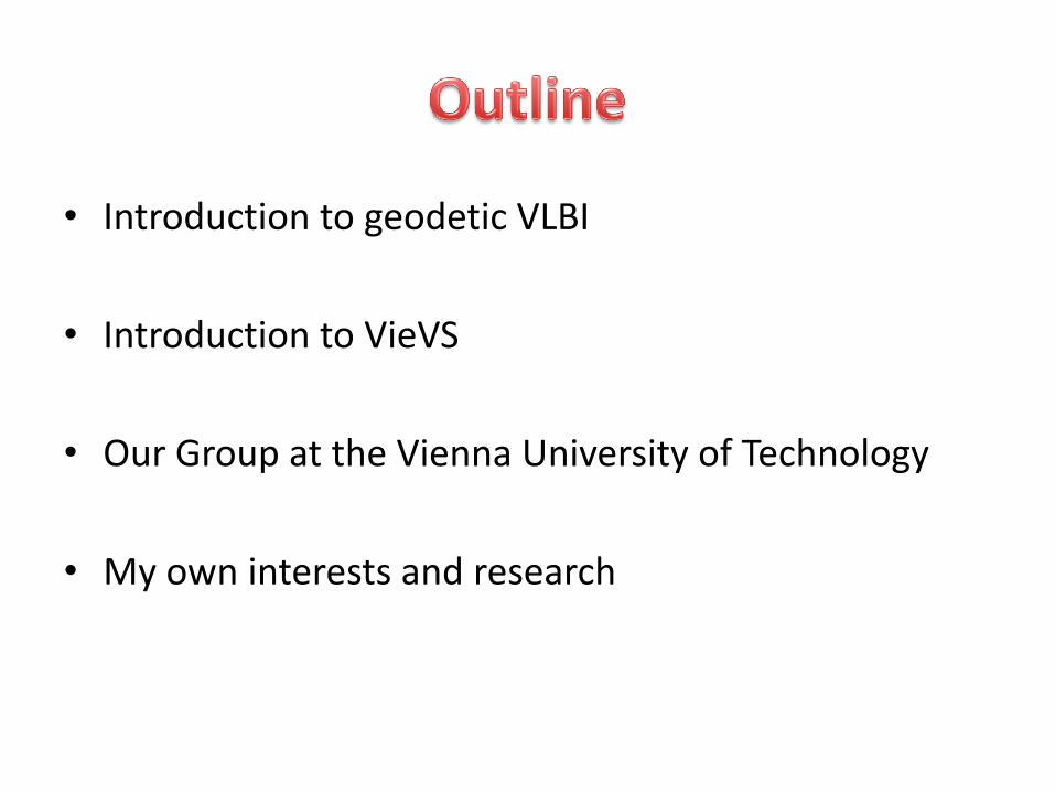
• Introduction to geodetic VLBI

• Introduction to VieVS

• Our Group at the Vienna University of Technology

• My own interests and research

Introduction to geodetic VLBI

Very Long Baseline Interferometry

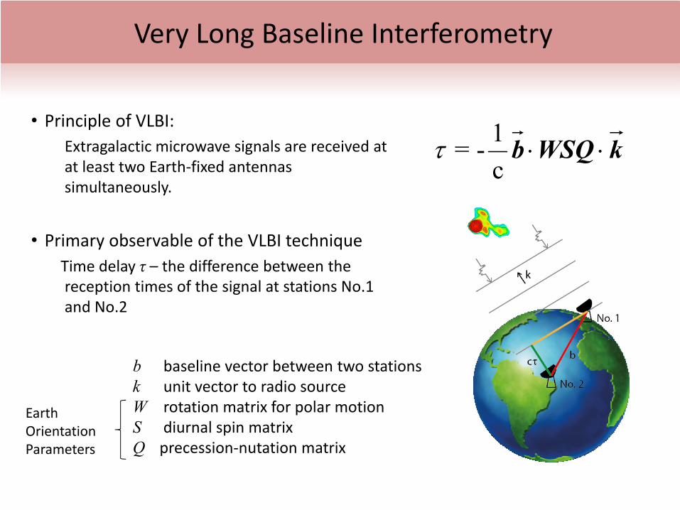
• Principle of VLBI:Extragalactic microwave signals are received at at least two Earth‐fixed antennas simultaneously.

• Primary observable of the VLBI techniqueTime delay τ – the difference between the reception times of the signal at stations No.1 and No.2

kWSQb ⋅⋅c1-=τ

b baseline vector between two stationsk unit vector to radio sourceW rotation matrix for polar motionS diurnal spin matrixQ precession‐nutation matrix

Earth Orientation Parameters

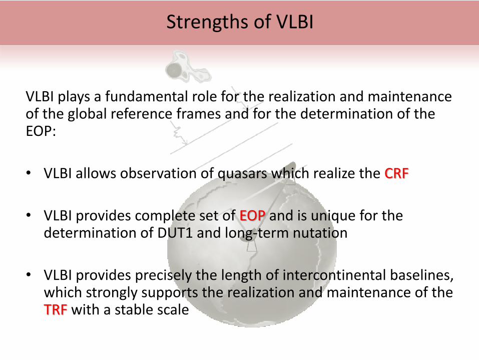
Strengths of VLBI

VLBI plays a fundamental role for the realization and maintenance of the global reference frames and for the determination of the EOP:

• VLBI allows observation of quasars which realize the CRF

• VLBI provides complete set of EOP and is unique for the determination of DUT1 and long‐term nutation

• VLBI provides precisely the length of intercontinental baselines, which strongly supports the realization and maintenance of the TRF with a stable scale

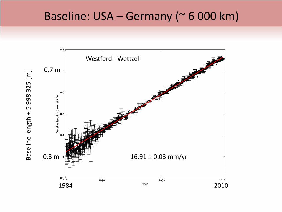
Baseline: USA – Germany (~ 6 000 km)

1984 2010

16.91 ± 0.03 mm/yr0.3 m

0.7 m

Westford ‐Wettzell

Baseline length + 5 998

 325

 [m]

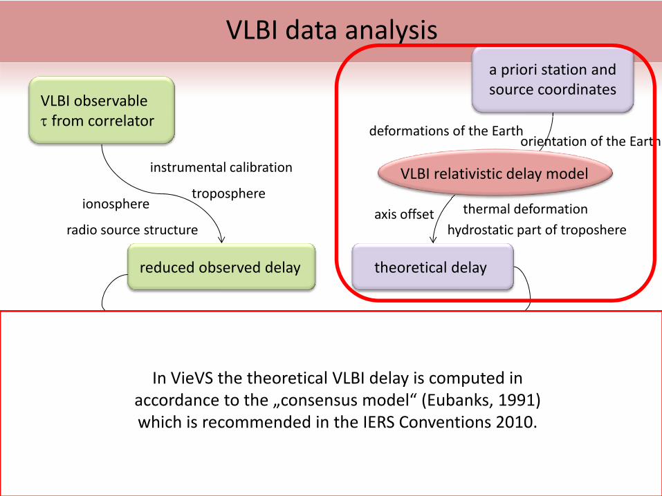
VLBI observableτ from correlator

reduced observed delay

instrumental calibration

troposphereionosphere

radio source structure

a priori station and source coordinates 

theoretical delay

VLBI relativistic delay model

deformations of the Earthorientation of the Earth

least squares adjustment

single session solution global solution

thermal deformationaxis offsethydrostatic part of troposhere

station coordinatesEOPposition of radio sources

troposphere estimatesclock parameters…

terrestrial reference framecelestial reference framegeodynamic parametersastronomical parameters…

VLBI data analysis

In VieVS the theoretical VLBI delay is computed in accordance to the „consensus model“ (Eubanks, 1991) which is recommended in the IERS Conventions 2010.

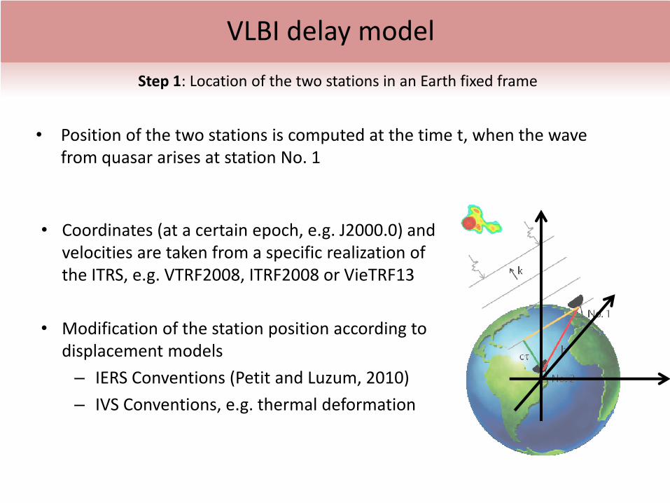
VLBI delay model

• Position of the two stations is computed at the time t, when the wave from quasar arises at station No. 1

• Coordinates (at a certain epoch, e.g. J2000.0) and velocities are taken from a specific realization of the ITRS, e.g. VTRF2008, ITRF2008 or VieTRF13

• Modification of the station position according to displacement models – IERS Conventions (Petit and Luzum, 2010)– IVS Conventions, e.g. thermal deformation

Step 1: Location of the two stations in an Earth fixed frame

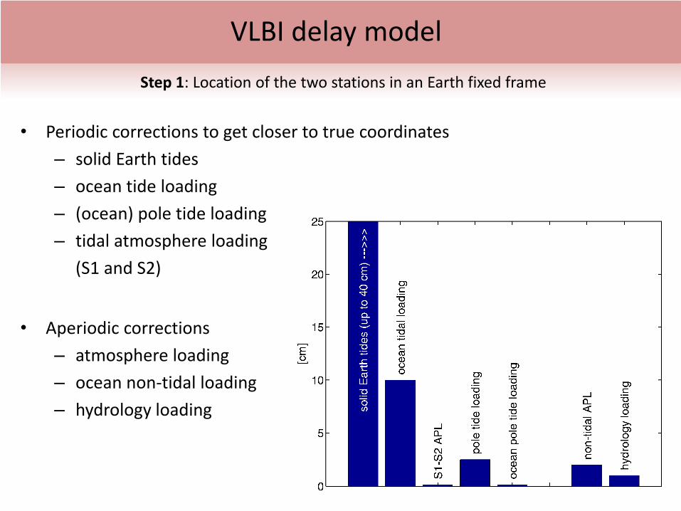
• Periodic corrections to get closer to true coordinates– solid Earth tides– ocean tide loading– (ocean) pole tide loading– tidal atmosphere loading

(S1 and S2)

• Aperiodic corrections– atmosphere loading– ocean non‐tidal loading– hydrology loading

VLBI delay modelStep 1: Location of the two stations in an Earth fixed frame

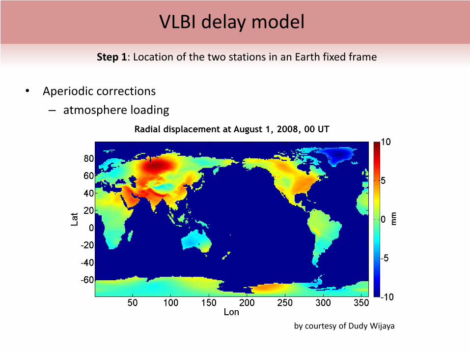
• Aperiodic corrections– atmosphere loading

Radial displacement at August 1, 2008, 00 UT

mm

by courtesy of Dudy Wijaya

VLBI delay modelStep 1: Location of the two stations in an Earth fixed frame

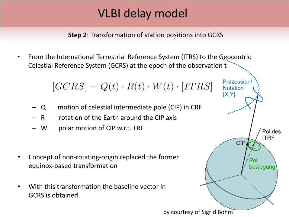
• From the International Terrestrial Reference System (ITRS) to the Geocentric Celestial Reference System (GCRS) at the epoch of the observation t

– Q motion of celestial intermediate pole (CIP) in CRF– R rotation of the Earth around the CIP axis– W polar motion of CIP w.r.t. TRF

VLBI delay modelStep 2: Transformation of station positions into GCRS

• Concept of non‐rotating‐origin replaced the former equinox‐based transformation

• With this transformation the baseline vector in GCRS is obtained

by courtesy of Sigrid Böhm

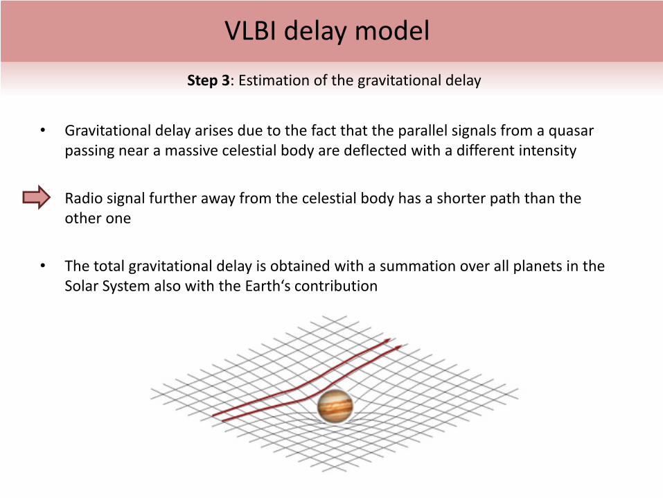
• Gravitational delay arises due to the fact that the parallel signals from a quasar passing near a massive celestial body are deflected with a different intensity

• Radio signal further away from the celestial body has a shorter path than the other one

• The total gravitational delay is obtained with a summation over all planets in the Solar System also with the Earth‘s contribution

VLBI delay modelStep 3: Estimation of the gravitational delay

by courtesy of Lucia Plank

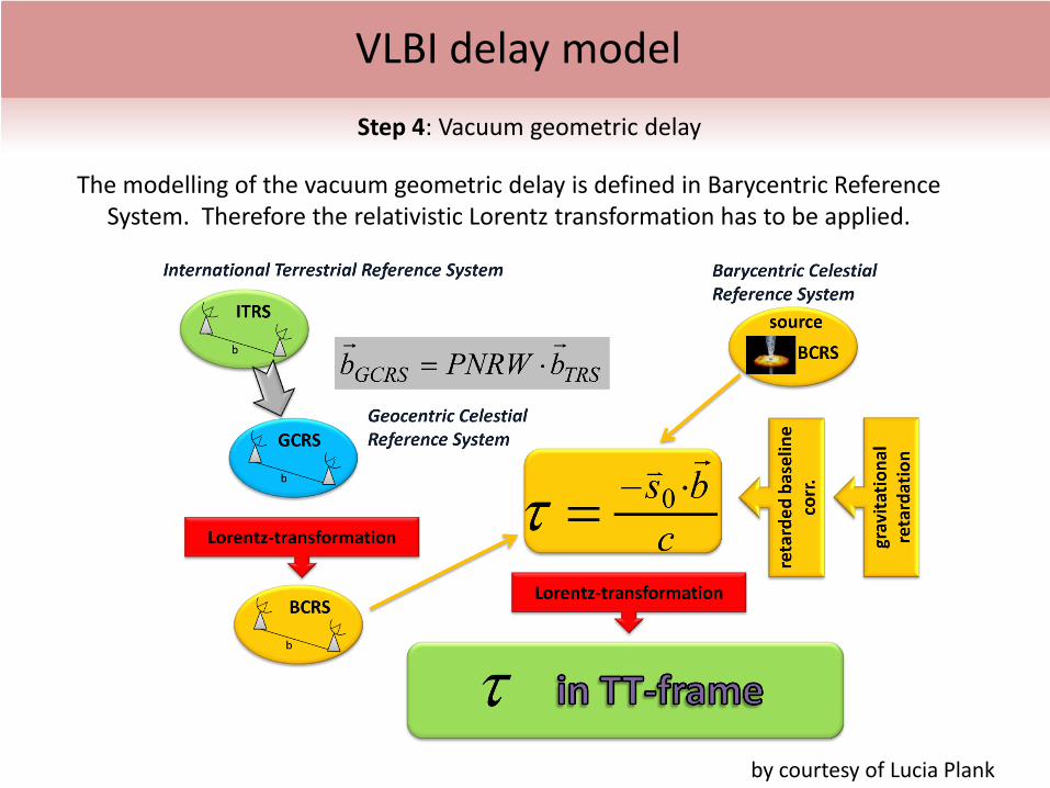
VLBI delay modelStep 4: Vacuum geometric delay

The modelling of the vacuum geometric delay is defined in Barycentric Reference System.  Therefore the relativistic Lorentz transformation has to be applied.

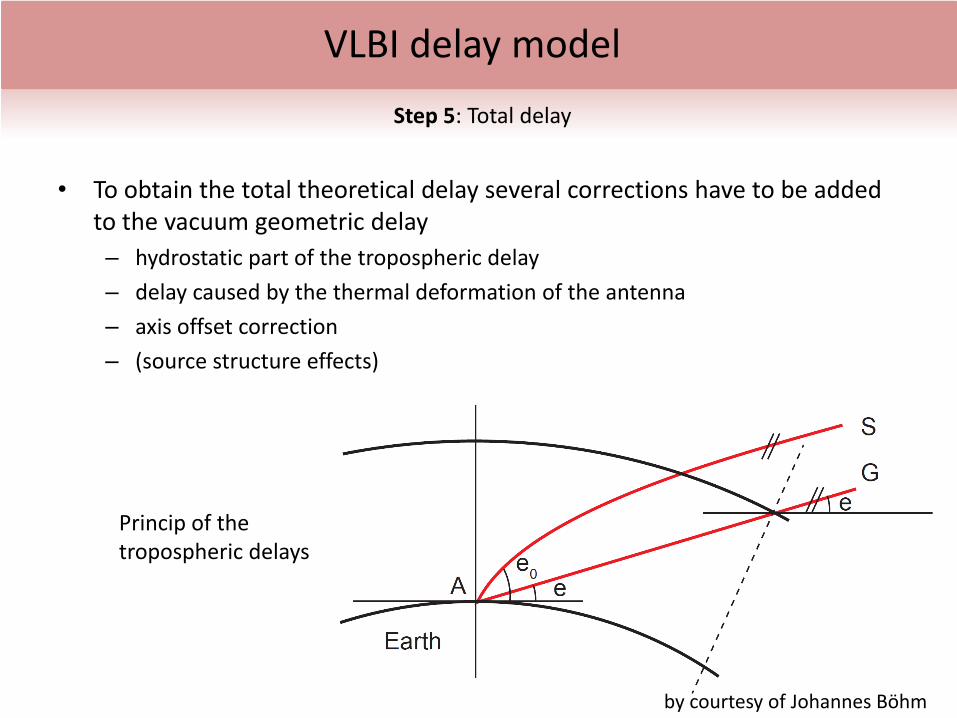
• To obtain the total theoretical delay several corrections have to be added to the vacuum geometric delay– hydrostatic part of the tropospheric delay– delay caused by the thermal deformation of the antenna– axis offset correction– (source structure effects)

VLBI delay modelStep 5: Total delay

by courtesy of Johannes Böhm

Princip of the tropospheric delays

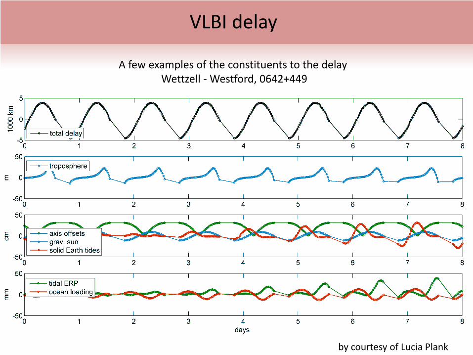
VLBI delay

A few examples of the constituents to the delayWettzell ‐Westford, 0642+449

by courtesy of Lucia Plank

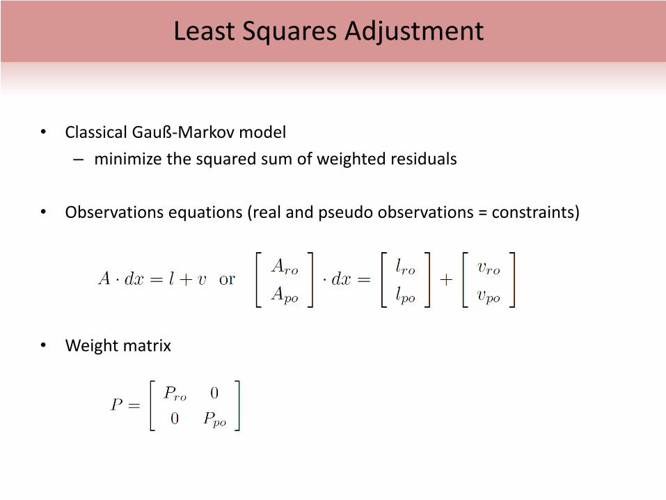
• Classical Gauß‐Markov model– minimize the squared sum of weighted residuals

• Observations equations (real and pseudo observations = constraints)

• Weight matrix

Least Squares Adjustment

• Two kinds of parameters

– parameters connected only with one observation session, they are changing in time (clock parameters, zenith wet delays, tropospheric gradients, EOP)

– parameters constant in time, so‐called global parameters,they are determined from a large number of sessions (TRF, CRF, geophysical or astronomic parameters)

• Parameters are modelled as piecewise linear offsets at e.g. integer hours... allows combination with other space geodetic techniques at normal equation level

Least Squares Adjustment

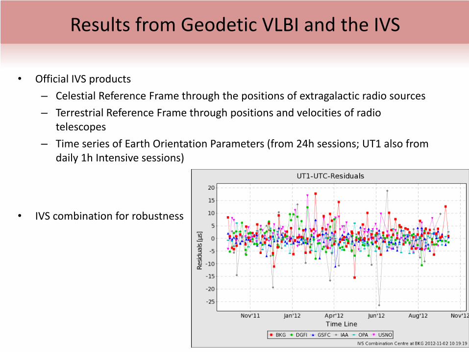
• Official IVS products– Celestial Reference Frame through the positions of extragalactic radio sources– Terrestrial Reference Frame through positions and velocities of radio 

telescopes– Time series of Earth Orientation Parameters (from 24h sessions; UT1 also from 

daily 1h Intensive sessions)

• IVS combination for robustness

Results from Geodetic VLBI and the IVS

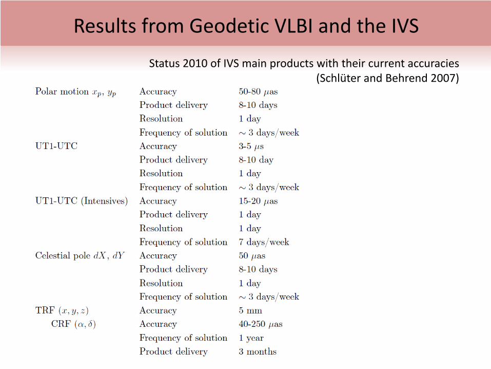
Results from Geodetic VLBI and the IVS

Status 2010 of IVS main products with their current accuracies (Schlüter and Behrend 2007)

• Geodetic VLBI can provide more parameters, like

– Love numbers of solid Earth tides

– ionosphere models

– troposphere parameters• long‐term VLBI zenith wet delays for climate studies• regression coefficients for atmospheric loading

– gravitational deflection of radio waves (gamma)

– acceleration of solar system barycentre

Results from Geodetic VLBI and the IVS

What is VieVS?

• VieVS = Vienna VLBI Software• A new, state of the art, geodetic VLBI data analysis software package• Written in Matlab• Since 2008 it is developed at the Department of Geodesy and Geoinformation

(Research Group Advanced Geodesy), Vienna University of Technology• Close cooperation with former colleagues (University of Tasmania,  Hacettepe

University in Turkey, Shanghai Astronomical Observatory)

• Current reference: Böhm J., S. Böhm, T. Nilsson, A. Pany, L. Plank, H. Spicakova, K. Teke, H. Schuh (2012).The New Vienna VLBI Software VieVS. Proceedings of the 2009 IAG Symposium, Series: International Association of Geodesy Symposia. Vol. 136. Geodesy for Planet Earth. Steve Kenyon, Maria Christina Pacino and Urs Marti (Eds.). ISBN 978‐3‐642‐20337‐4. pp. 1007‐1011.DOI: 10.1007/978‐3‐642‐20338‐1_126 .

• Important that there exist several different types of VLBI analysis software

• Different software packages can validate each other. Helps identifying bugs etc.

• Analysts have a choice of what to use

• VLBI2010 / VGOS put new demands and challenges on the VLBI analysis software

• We want to have a VLBI software which is easy to use:– BSc, MSc, and PhD students can easily learn it and use it– Should be easy to add new models etc. for special investigations– Graphical User Interface (GUI)– Should have a clear structure

Why did we develop VieVS?

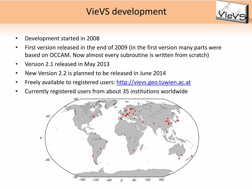
• Development started in 2008• First version released in the end of 2009 (In the first version many parts were 

based on OCCAM. Now almost every subroutine is written from scratch)• Version 2.1 released in May 2013• New Version 2.2 is planned to be released in June 2014• Freely available to registered users: http://vievs.geo.tuwien.ac.at• Currently registered users from about 35 institutions worldwide

VieVS development

• Advantages:– Easy to use– Easy to change source code– Good tools for plotting etc.– Matlab available on all major operating systems (Windows, 

Linux/UNIX, Mac OS)

• Disadvantages:– Matlab is an expensive commercial software

(VieVS is in principle working on GNU Octave, but without GUI and it is much slower; Qt Interface (V. Choliy) )

– Slower than C++ or Fortran. Not a major problem.

Why Matlab

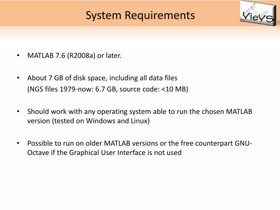
System Requirements

• MATLAB 7.6 (R2008a) or later.

• About 7 GB of disk space, including all data files(NGS files 1979‐now: 6.7 GB, source code: <10 MB)

• Should work with any operating system able to run the chosen MATLAB version (tested on Windows and Linux)

• Possible to run on older MATLAB versions or the free counterpart GNU‐Octave if the Graphical User Interface is not used

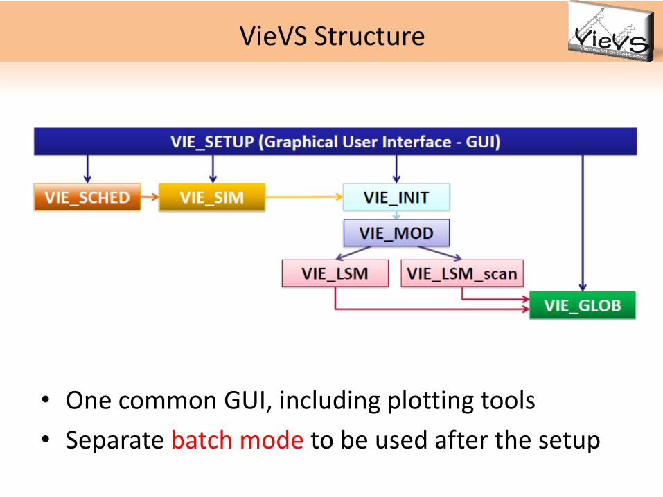
VieVS Structure

• One common GUI, including plotting tools• Separate batch mode to be used after the setup

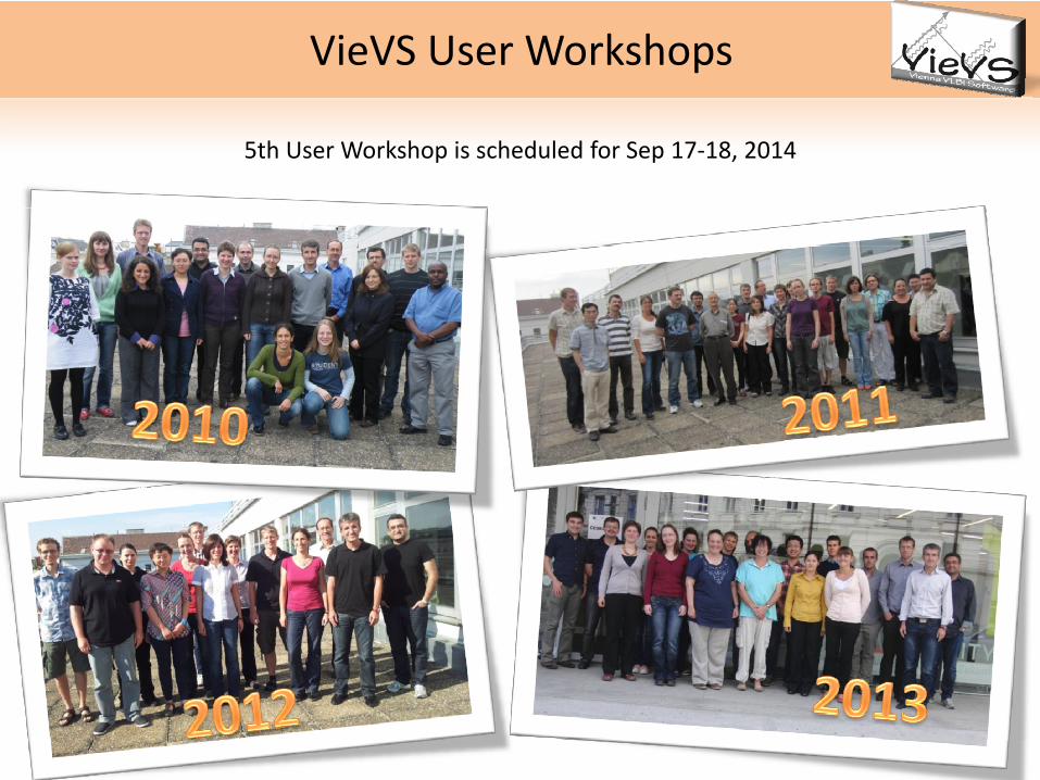
VieVS User Workshops

5th User Workshop is scheduled for Sep 17‐18, 2014

Our Group at theVienna University of Technology

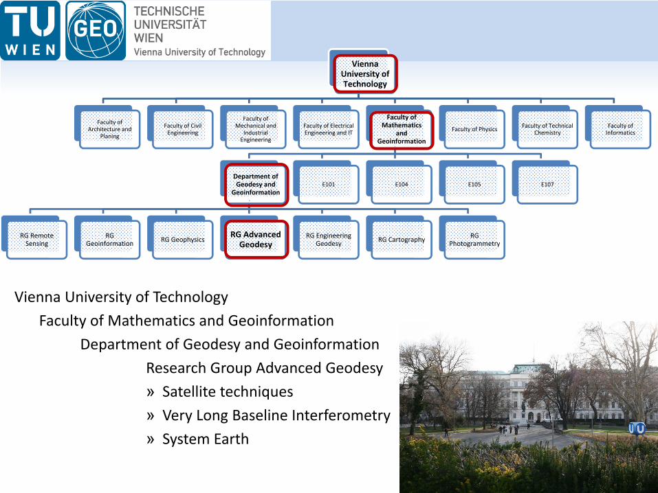
Vienna University of Technology

Faculty of Architecture and 

Planing

Faculty of Civil Engineering

Faculty of Mechanical and 

Industrial Engineering

Faculty of Electrical Engineering and IT

Faculty of Mathematics 

and Geoinformation

Department of Geodesy and 

Geoinformation

RG Remote Sensing

RG Geoinformation RG Geophysics RG Advanced 

GeodesyRG Engineering 

Geodesy RG Cartography RG Photogrammetry

E101 E104 E105 E107

Faculty of Physics Faculty of Technical Chemistry

Faculty of Informatics

Vienna University of TechnologyFaculty of Mathematics and Geoinformation

Department of Geodesy and GeoinformationResearch Group Advanced Geodesy » Satellite techniques» Very Long Baseline Interferometry» System Earth

Current VLBI Group in Vienna (April 2014) Alphabetically

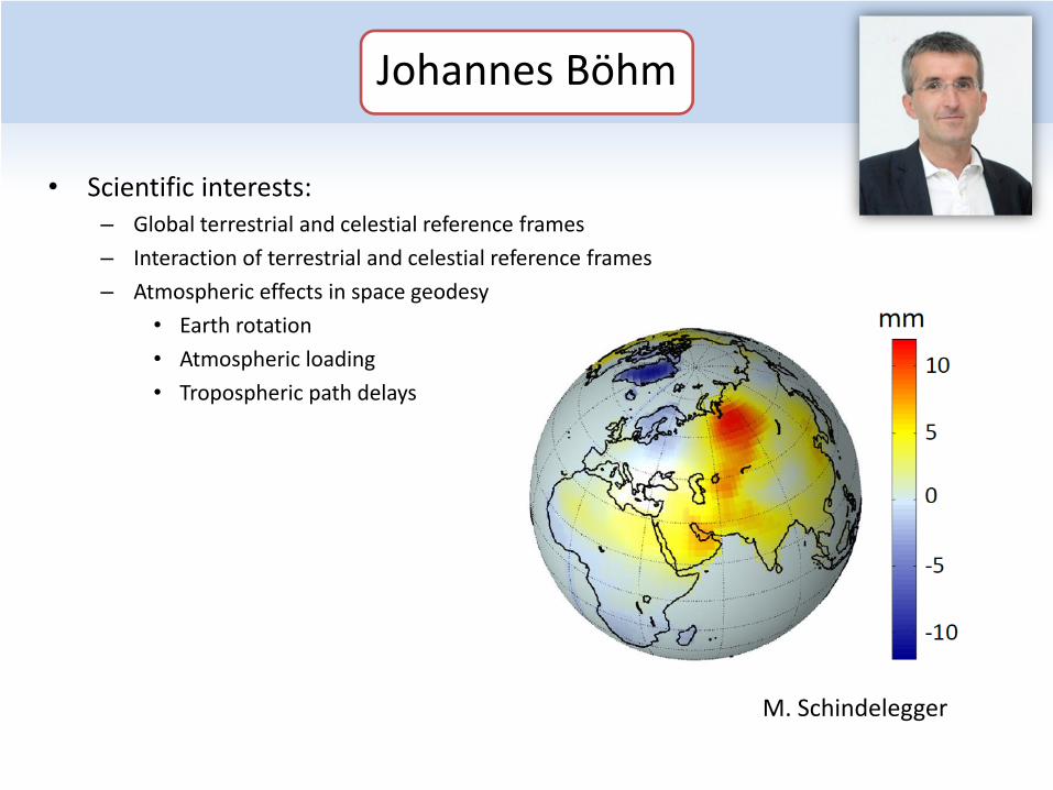
Johannes Böhm

• Scientific interests:– Global terrestrial and celestial reference frames– Interaction of terrestrial and celestial reference frames– Atmospheric effects in space geodesy

• Earth rotation• Atmospheric loading• Tropospheric path delays

M. Schindelegger

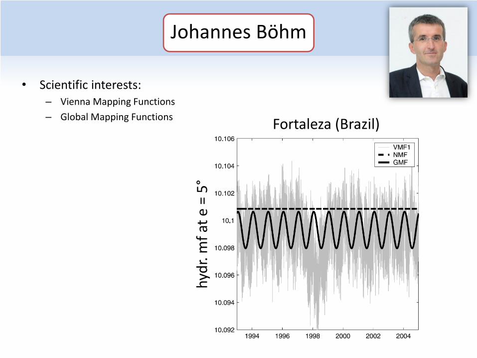
Johannes Böhm

• Scientific interests:– Vienna Mapping Functions– Global Mapping Functions Fortaleza (Brazil) 

hydr. m

f at e

 = 5°

Johannes Böhm

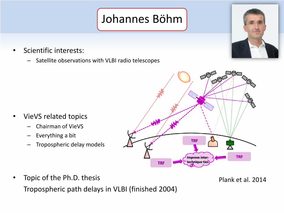
• Scientific interests:– Satellite observations with VLBI radio telescopes

• VieVS related topics– Chairman of VieVS– Everything a bit– Tropospheric delay models

• Topic of the Ph.D. thesisTropospheric path delays in VLBI (finished 2004)

Plank et al. 2014

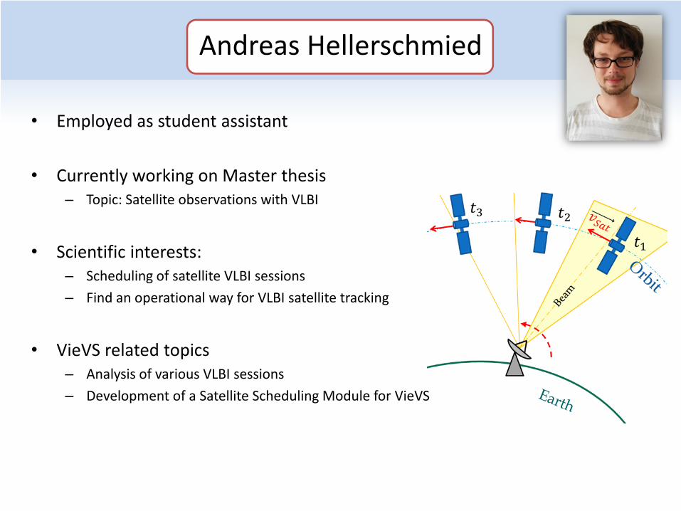
Andreas Hellerschmied

• Employed as student assistant

• Currently working on Master thesis– Topic: Satellite observations with VLBI

• Scientific interests:– Scheduling of satellite VLBI sessions– Find an operational way for VLBI satellite tracking

• VieVS related topics– Analysis of various VLBI sessions– Development of a Satellite Scheduling Module for VieVS

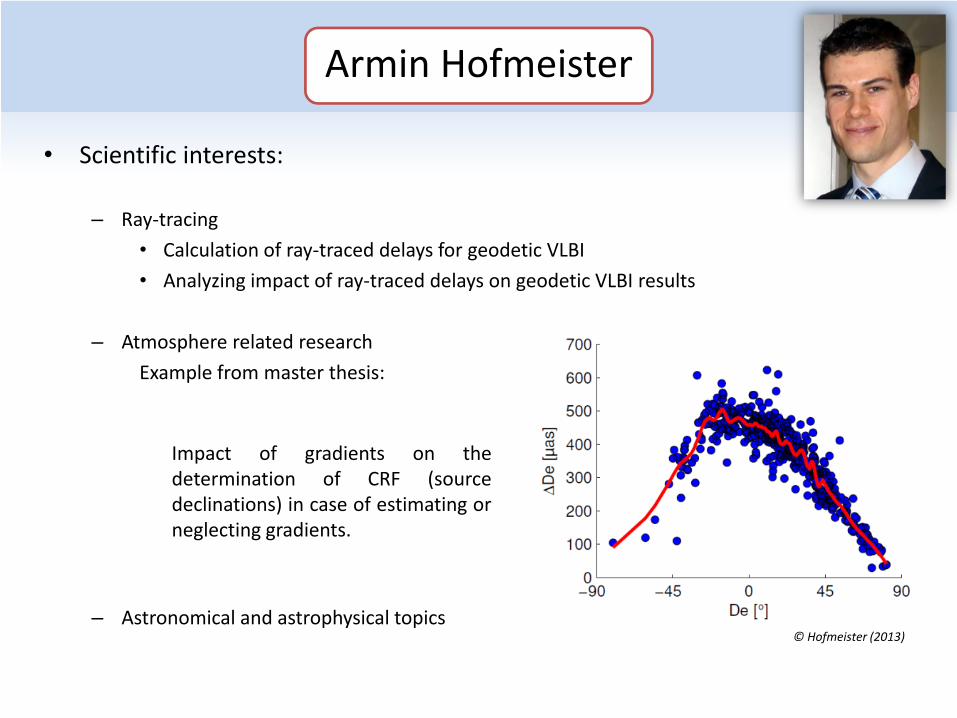
Armin Hofmeister

• Scientific interests:

– Ray‐tracing• Calculation of ray‐traced delays for geodetic VLBI• Analyzing impact of ray‐traced delays on geodetic VLBI results

– Atmosphere related researchExample from master thesis:

– Astronomical and astrophysical topics© Hofmeister (2013)

Impact of gradients on thedetermination of CRF (sourcedeclinations) in case of estimating orneglecting gradients.

Armin Hofmeister

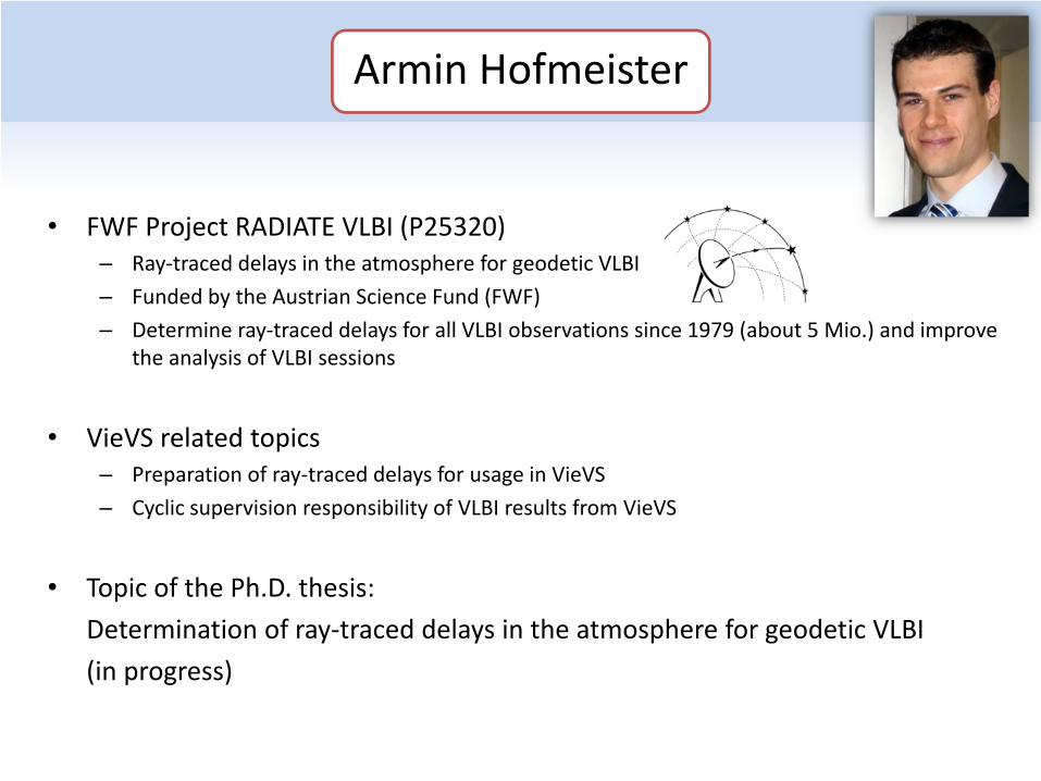
• FWF Project RADIATE VLBI (P25320)– Ray‐traced delays in the atmosphere for geodetic VLBI– Funded by the Austrian Science Fund (FWF)– Determine ray‐traced delays for all VLBI observations since 1979 (about 5 Mio.) and improve 

the analysis of VLBI sessions

• VieVS related topics– Preparation of ray‐traced delays for usage in VieVS– Cyclic supervision responsibility of VLBI results from VieVS

• Topic of the Ph.D. thesis:Determination of ray‐traced delays in the atmosphere for geodetic VLBI(in progress)

Hana Krásná

• Scientific interests:– Displacement of reference points, loading effects– Reference frames

• Computation of Vienna Reference Frames, current version: VieTRF13, VieCRF13• Submission of a VLBI solution for ITRF2013

– Various global parameters from VLBI (Love and Shida numbers, FCN period, axis offset, …)

• VieVS related topics– Development of Vie_MOD (together with Lucia Plank) and Vie_GLOB– Organisation of VieVS Workshops– Maintenance of our VieVS server

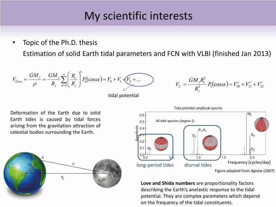
• Topic of the Ph.D. thesisEstimation of solid Earth tidal parameters and FCN with VLBI (finished Jan 2013)

Younghee Kwak

• Scientific interests:– Combination of Space Geodetic Techniques– Reference Frames and EOP– Plate tectonics

• VieVS related topics– Simulation of global GPS‐VLBI hybrid observation

• Topic of the Ph.D. thesisDevelopment and validation experiment of the GPS‐VLBI hybrid system (finished Feb 2011)

Matthias Madzak

• Scientific interests:– Geophysical excitation of Earth rotation– Ocean tides, Hydrodynamics– Atmospheric effects

• VieVS related topics– Development of Vie_SETUP (Graphical User Interface) of VieVS– External files (ionospheric, tropospheric, superstation, supersource)– Data format and data structure (openDB)– Plotting and output – analysis support

• Topic of the Ph.D. thesisShort period ocean tidal variations in Earth rotation (to be finished 2014)

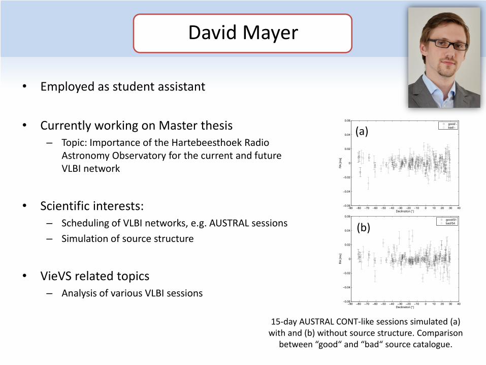
David Mayer

• Employed as student assistant

• Currently working on Master thesis– Topic: Importance of the Hartebeesthoek Radio 

Astronomy Observatory for the current and future VLBI network

• Scientific interests:– Scheduling of VLBI networks, e.g. AUSTRAL sessions– Simulation of source structure

• VieVS related topics– Analysis of various VLBI sessions

−90 −80 −70 −60 −50 −40 −30 −20 −10 0 10 20 30 40−0.06

−0.04

−0.02

0

0.02

0.04

0.06

RA

[ms]

Declination [°]

good/−bad/−

−90 −80 −70 −60 −50 −40 −30 −20 −10 0 10 20 30 40−0.06

−0.04

−0.02

0

0.02

0.04

0.06

RA

[ms]

Declination [°]

good/S1bad/S4

15‐day AUSTRAL CONT‐like sessions simulated (a) with and (b) without source structure. Comparison 

between “good“ and “bad“ source catalogue.

(a)

(b)

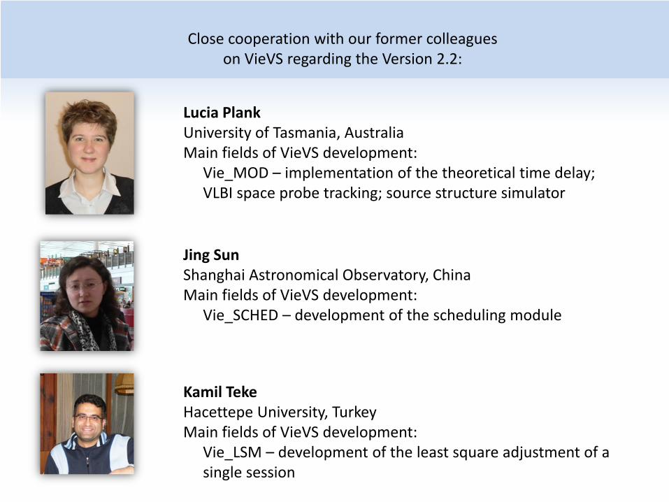
Close cooperation with our former colleagues on VieVS regarding the Version 2.2:

Lucia PlankUniversity of Tasmania, AustraliaMain fields of VieVS development:

Vie_MOD – implementation of the theoretical time delay; VLBI space probe tracking; source structure simulator

Jing SunShanghai Astronomical Observatory, ChinaMain fields of VieVS development:

Vie_SCHED – development of the scheduling module

Kamil TekeHacettepe University, TurkeyMain fields of VieVS development:

Vie_LSM – development of the least square adjustment of a single session

• Topic of the Ph.D. thesisEstimation of solid Earth tidal parameters and FCN with VLBI (finished Jan 2013)

Deformation of the Earth due to solidEarth tides is caused by tidal forcesarising from the gravitation attraction ofcelestial bodies surrounding the Earth.

( ) ...cos 2100

+++=⎟⎟⎠

⎞⎜⎜⎝

⎛== ∑

∞

=

VVVPRR

RGMGM

Vn

n

n

j

e

j

jjGrav α

ρ

tidal potential 

( ) ttt

j

ej VVVPRRGM

V 22212023

2

2 cos ++== α

Figure adapted from Agnew (2007)long‐period tides diurnal tides Frequency [cycles/day]

Love and Shida numbers are proportionality factors describing the Earth’s anelastic response to the tidal potential. They are complex parameters which depend on the frequency of the tidal constituents.

My scientific interests

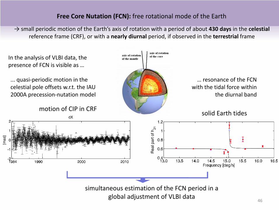
solid Earth tidesmotion of CIP in CRF

simultaneous estimation of the FCN period in a global adjustment of VLBI data

... quasi‐periodic motion in the celestial pole offsets w.r.t. the IAU 2000A precession‐nutation model

… resonance of the FCN with the tidal force within 

the diurnal band

In the analysis of VLBI data, the presence of FCN is visible as …

46

Free Core Nutation (FCN): free rotational mode of the Earth

→ small periodic motion of the Earth’s axis of rotation with a period of about 430 days in the celestial reference frame (CRF), or with a nearly diurnal period, if observed in the terrestrial frame

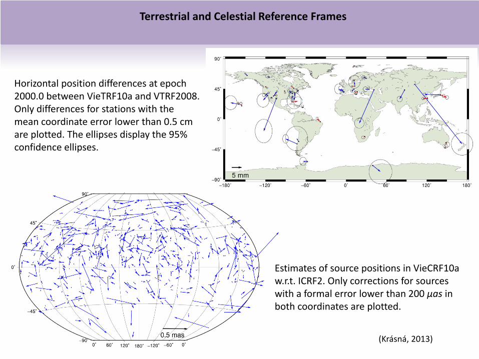
Terrestrial and Celestial Reference Frames

(Krásná, 2013)

Horizontal position differences at epoch 2000.0 between VieTRF10a and VTRF2008.Only differences for stations with the mean coordinate error lower than 0.5 cm are plotted. The ellipses display the 95% confidence ellipses.

Estimates of source positions in VieCRF10a w.r.t. ICRF2. Only corrections for sources with a formal error lower than 200 μas in both coordinates are plotted.

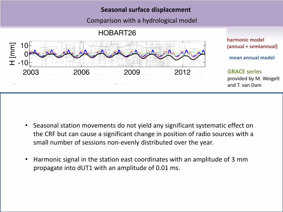
Comparison with a hydrological model

48

FORTLEZA  0.41   0.71 NYALES20  0.20    0.09HARTRAO   0.23 0.10  TIGOCONC  0.73    0.64HOBART26  0.66   0.71      TSUKUB32    0.34    0.21KOKEE  0.14 0.33 WESTFORD   0.41    0.59MATERA          0.70  0.67  WETTZELL     0.73    0.74

correl. coeff.

mean annual model 

harmonic model (annual + semiannual)

GRACE seriesprovided by M. Weigeltand T. van Dam

Hydrology loading displacementprovided by GSFC group, D.Eriksson; computed from the monthly GLDAS NOAH model

correl. coeff.

Seasonal surface displacement

• Seasonal station movements do not yield any significant systematic effect on the CRF but can cause a significant change in position of radio sources with a small number of sessions non‐evenly distributed over the year.

• Harmonic signal in the station east coordinates with an amplitude of 3 mm propagate into dUT1 with an amplitude of 0.01 ms.

Thank you for your attention!