PHASE VERSUS DELAY IN GEODETIC VLBI …...PHASE VERSUS DELAY IN GEODETIC VLBI James Campbell Geodetic Institute University of Bonn ABSTRACT For high precise baseline and source position

PHASE VERSUS DELAY IN GEODETIC VLBI

James Campbell

Geodetic Institute University of Bonn

ABSTRACT

For high precise baseline and source position determinations with VLBI, large bandwidth techniques are required to achieve the necessary delay resolution of S 0.1 ns. In local interferometry, the interferometric phase observable offers an equally high resolution in spite of the much smaller bandwidths used. In the present paper, the conditions for the applicability of the phase observable in very long baseline interferometry (VLBI) are discussed and examples of adequate observation programs are given. These considerations apply in particular to the Mark II system, which is already in operation at many observatories.

385

https://ntrs.nasa.gov/search.jsp?R=19800020335 2020-05-08T09:23:40+00:00Z

386 RADIO INTERFEROMETRY

DELAY AND PHASE OBSERVATIONS

In radio interferometry the travelling time r of a wavefront between the antennas at two sites is measured by maximizing the cross-correlation function of the two signal streams received at the two antennas. Simultaneously, .the phase and the rate of the interference fringes are determined in the processor as they vary with the Earth’s rotation. During correlation, the data stream from one sta- tion is delayed quasi-continuously in such a way that the changing geometric delay 7s is almost completely compensated for. This gives rise to a rather low residual fringe frequency the phase of which slowly varies on the scale of a few turns per minute. In order to be able to observe those fringes which have maximum amplitude, the correlation is carried out simultaneously in a number of delay channels separated by

1 AT = -

2 Bo (1)

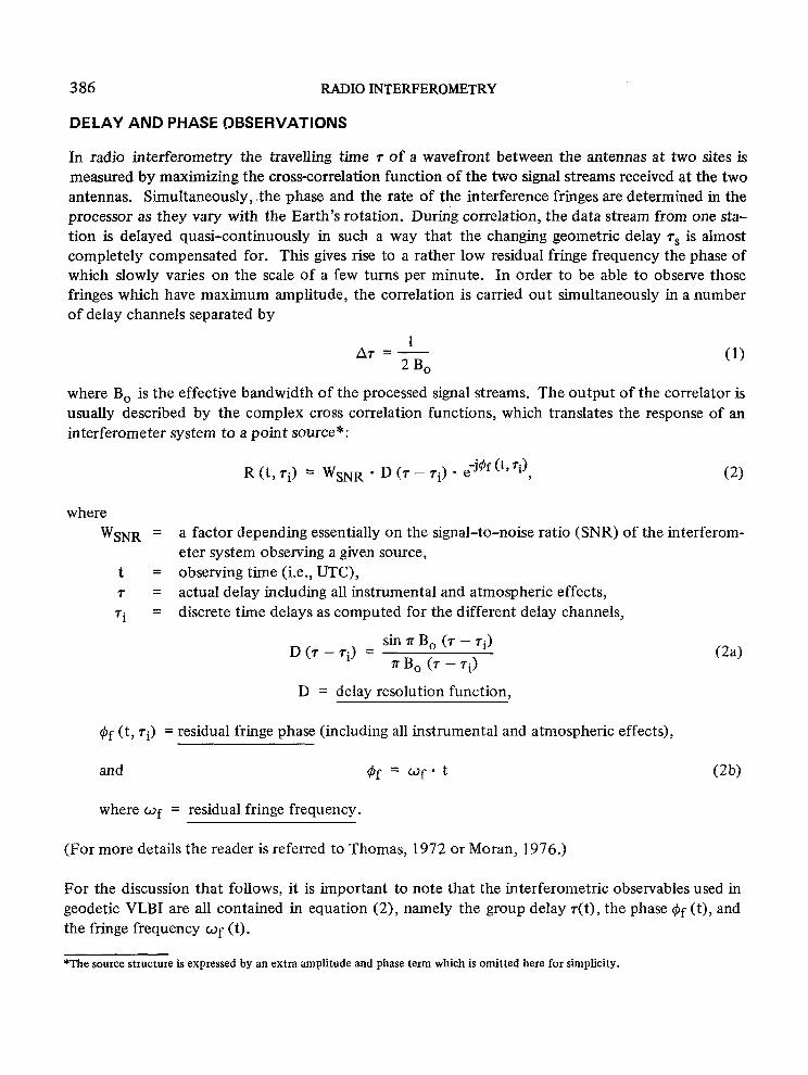
where B, is the effective bandwidth of the processed signal streams. The output of the correlator is usually described by the complex cross correlation functions, which translates the response of an interferometer system to a point source*:

R (t, Ti) -jGf (t, 7i) = WSNR l D (r - ri) * e , (2)

where

WSNR = a factor depending essentially on the signal-to-noise ratio (SNR) of the interferometer system observing a given source,

t = observing time (i.e., UTC), 7 = actual delay including all instrumental and atmospheric effects,

Ti = discrete time delays as computed for the different delay channels,

D (7 - ri) = sin a B, (T - Ti) 7T Bo (7 - 71)

D = delay resolution function,

@f (t, 71) = residual fringe phase (including all instrumental and atmospheric effects),

and $f = Wf l t

(2a)

(2b)

where Of = residual fringe frequency.

(For more details the reader is referred to Thomas, 1972 or Moran, 1976.)

For the discussion that follows, it is important to note that the interferometric observables used in geodetic VLBI are all contained in equation (2), namely the group delay r(t), the phase $f (t), and the fringe frequency Wf (t).

*The source structure is expressed by an extra amplitude and phase term which is omitted here for simplicity.

WAVES OF THE FUTURE AND OTHER EMISSIONS 387

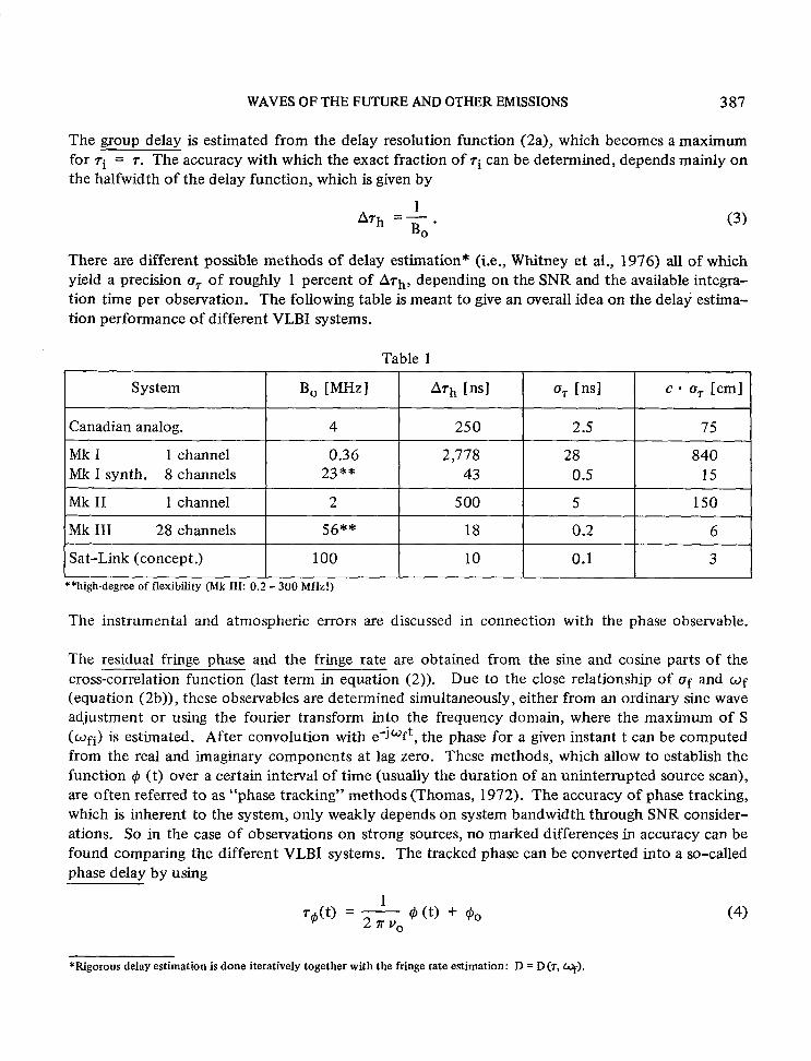
The group delay is estimated from the delay resolution function (2a), which becomes a maximum for 71 = 7. The accuracy with which the exact fraction of ri can be determined, depends mainly on the halfwidth of the delay function, which is given by

Arh =$. 0

(3)

There are different possible methods of delay estimation* (i.e., Whitney et al., 1976) all of which yield a precision c7 of roughly 1 percent of Arh, depending on the SNR and the available integra- tion time per observation. The following table is meant to give an overall idea on the delay estimation performance of different VLBI systems.

Table 1

**high-degree of flexibility (Mk III: 0.2 - 300 MHz!)

The instrumental and atmospheric errors are discussed in connection with the phase observable.

The residual fringe phase and the fringe rate are obtained from the sine and cosine parts of the cross-correlation function (last term in equation (2)). Due to the close relationship of uf and wf (equation (2b)), these observables are determined simultaneously, either from an ordinary sine wave adjustment or using the fourier transform into the frequency domain, where the maximum of S (Wfi) is estimated. After convolution with edwft, the phase for a given instant t can be computed from the real and imaginary components at lag zero. These methods, which allow to establish the function @ (t) over a certain interval of time (usually the duration of an uninterrupted source scan), are often referred to as “phase tracking” methods (Thomas, 1972). The accuracy of phase tracking, which is inherent to the system, only weakly depends on system bandwidth through SNR considerations. So in the case of observations on strong sources, no marked differences in accuracy can be found comparing the different VLBI systems. The tracked phase can be converted into a so-called phase delay by using

1 rdt) - 2 xv0 - - d (0 + f$o (4)

*Rigorous delay estimation is done iteratively together with the fringe rate estimation: D = D(T, 9).


where ve = center of observing frequency band, and

$0 = constant phase zero term, accounting for the unknown number of turns at the start of each source scan.

The phase delay accuracy, which is equivalent to the phase accuracy, is composed of the small phase tracking error plus the much larger instrumental and atmospheric phase errors listed below:

- clock stability (phase variations of the local oscillators) - instrumental delay (electronics, cables + mechanical structure) - atmospheric delay (ionosphere; troposphere, dry and wet) - resolved sources add phase variations due to their structure.

Typical phase tracking errors on strong sources are about one-tenth of a turn or smaller; this translates into phase delay errors of some tens of picoseconds only, corresponding to the observing frequency used. The overall phase variations due to the above mentioned effects, however, amount to about 0.1 ns (if hydrogen masers are used as frequency standards). It is difficult to give a represen- tative number here because of the wide variability of atmospheric and instrumental conditions. It may be possible in the near future to reduce this number by a factor of two or three using satellite LO links, instrumental delay calibration, dual-frequency receiving systems and water vapor radiom- etry. But even in the less favourable case of 07@ = 0.1 ns, the phase delay accuracy of any narrow band system is equivalent to a group delay precision of a wide bandwidth system with B, = 100 MHz.

What can be done to take advantage of the phase observables for meaningful geodetic work, will be shown in the next paragraphs.

GEODETIC BASELINE DETERMINATIONS USING PHASE OBSERVATIONS

There are several ways in which phase observations are made following the purpose of the experiment.

Method A: Uninterrupted Scans for Mapping the Structure of Compact Radio Sources

In most of these experiments the telescopes are aimed at the same source for many hours, with the exception of a few short calibration scans. During each of these scans, the phase can be tracked without ambiguity problems, even at higher frequencies, as long as interference fringes are seen.

For a unique baseline solution with this kind of data, the following conditions have to be met:

1. The polar component (z = component) of the baseline has to be kept fixed. 2. At the start of each source scan, a new phase zero unknown (which is equal to a clock offset

unknown) has to be introduced.


3. The duration of the sources scans should not be shorter than 3 to 4 hours. An optimum is reached if the hour angle range covers 180” (z 12 hours).

These conditions can be deduced from the observation equations, where the baseline terms expressed in cylindrical coordinates are

dbl = +sin6 (polar component)

db2 = $ cos 6 cos h (equatorial component)

dhh = b2 - cos 6 sin h (longitude of baseline vector) C

with 6 = declination and h = hour angle of the observed source.

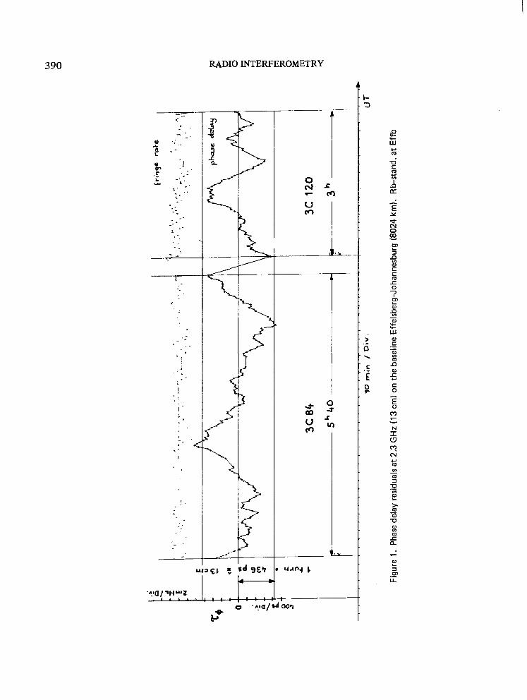
An example of a baseline solution with 13 cm data on an intercontinnetal baseline is shown in figure 1. These data are the first that could be used with a program completed only very recently. In spite of the poor quality of these data (rubidium clocks were used at both stations), a comparison with the delay solution of the same experiment demonstrates the substantial gain in accuracy:

delay solution :

*r = kg.5 ns dbl = 47.52 f 1.62 m

db2 = 16.00 f 2.86 m

dhb = 4’.‘97 * 0’.‘32

phase delay solution: dbl = - - -

% = 20.20 ns db2 = 19.32 f 0.24m

dXb = 4’.‘42 +- 0’.‘03

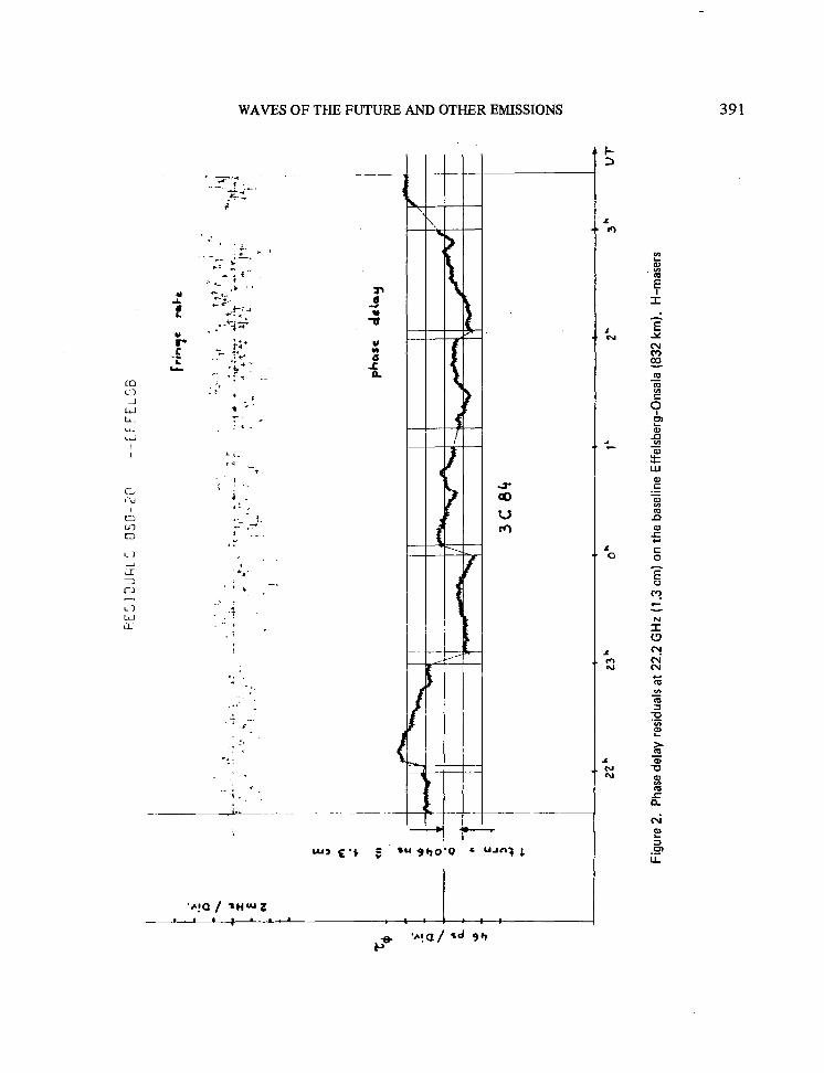
Another example is shown in figure 2, where phase data on the 832 km baseline Effelsberg-Onsala at 1.3 cm (22.2 GHz) were converted into phase delays. Due to the small ambiguity spacing at this high frequency, it proved to be difficult to connect the phases across data gaps larger than 5 minutes (coherence time of the interferometer).

The phase delay solution with scan on 3C273 and 3C84 gave the following results:

% = +0.15 ns db2 = 0.15 f 0.054m

dhb = 3’.‘3 6 +_ 0’.‘008

The drawback of method A, however, is twofold: the baseline solution is incomplete and only a few sources can be observed during one experiment. Moreover, very severe bounds have to be placed on the systematic effects due to the instrumentation and the atmosphere because there is a high sensitivity of these solutions to any non-linear effects in the phase delay observables.

3c

120

I----

-3h

- I

-i

Figu

re

1.

Phas

e de

lay

resi

dual

s at

2.3

GH

z (1

3 cm

) on

the

bas

elin

e Ef

fels

berg

-Joh

anne

sbur

g (8

024

km).

Rb-

stan

d.

at E

ffb

. : E

(Y

II c 3 3C

84

c

I

phw

dr

loy

; 9 f 0 -

.- 0

- 3

- 8

- - 2z

k t3

* O

h 1’

2’

3h

u-

l-

Figu

re 2

. Ph

ase

dela

y re

sidu

als

at 2

2.2

GH

z (1

.3 c

m)

on t

he b

asel

ine

Effe

lsbe

rg-O

nsal

a (8

32 k

m).

H-m

aser

s


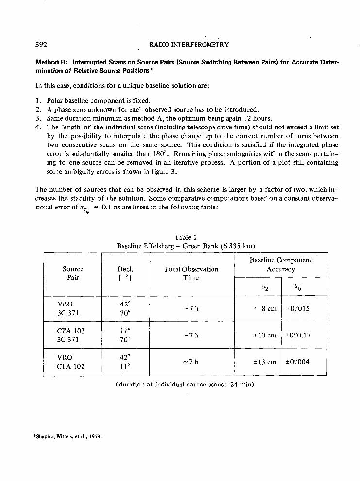
Method 6: Interrupted Scans on Source Pairs (Source Switching Between Pairs) for Accurate Deter- mination of Relative Source Positions*

In this case, conditions for a unique baseline solution are:

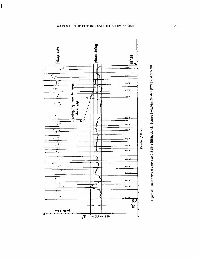
1. Polar baseline component is fixed. 2. A phase zero unknown for each observed source has to be introduced. 3. Same duration minimum as method A, the optimum being again 12 hours. 4. The length of the individual scans (including telescope drive time) should not exceed a limit set

by the possibility to interpolate the phase change up to the correct number of turns between two consecutive scans on the same source. This condition is satisfied if the integrated phase error is substantially smaller than 180”. Remaining phase ambiguities within the scans pertain- ing to one source can be removed in an iterative process. A portion of a plot still containing some ambiguity errors is shown in figure 3.

The number of sources that can be observed in this scheme is larger by a factor of two, which in- creases the stability of the solution. Some comparative computations based on a constant observa- tional error of 0

ro = 0.1 ns are listed in the following table:

Source Pair

VRO 3c 371

CTA 102 3c 371

VRO CTA 102

Table 2 Baseline Effelsberg - Green Bank (6 335 km)

Baseline Component Decl. Total Observation Accuracy 1 “3 Time

b2 lb

42” 70”

-7 h f 8cm *0:‘015

11” 70”

-7h +-10cm +0:‘0.17

42” 11”

-7 h +13 cm + OYOO4

(duration of individual source scans: 24 mm)

*Shapiro, Wittels, et al., 1979.

-5

f *

/ 1.

L

._-

I : .

P J

42’3

?

? i

- - I ” ;

- - z?!

- ! ;r -r

10 r

&n

/ D

ir.

Frin

,e ro

te

.

?

I L 18’ 5

8 I ph

ase

drlo

y

Figu

re 3

. Ph

ase

dela

y re

sidu

als

at 2

.3 G

Hz

(Effb

.-Job

.).

Sour

ce S

witc

hing

M

ode

(3C

273

and

3C27

9)


Method C: Interrupted Scans on Many Different Sources

The sampling of sources all over the commonly visible portion of the sky would, of course, provide the most stable least squares solution, a fact which can best be demonstrated by comparing the correlation matrices of methods A, B and C: unless the observation period is extended over 12 hours or more, the solutions of methods A and B tend to show strong correlations (0.9) between some of the estimated parameters. It is interesting, however, that the equatorial baseline projection b2 in all cases correlates only very weakly with the other parameters.

The realization of method C becomes increasingly difficult with an increasing number of sources involved in the switching scheme. This is easily understood because the gaps between scans on the same source widen considerably, preventing correct phase interpolation. In this case, more sophis- ticated methods of ambiguity elimination are required.

AMBIGUITY ELIMINATION

In order to obtain a complete baseline solution including the z-component, the remaining phase ambiguities between scans to different sources must be resolved. In Rogers et al., 1978 an interesting method of phase ambiguity elimination is described, which relies on a preliminary wide band delay solution. At the relatively high observing frequency of 7.85 GHz, one phase turn corresponds to an ambiguity spacing of 3.8 cm or 0.13 ns. This was roughly equivalent to the uncertainty of the adjusted group delay observations from the preliminary solution. Now these adjusted delay observations were converted to reference phases which were then subtracted from the observed phases. After suppression of clock drift effects, the phase differences were treated in a special function

f(g) = 2 COSA@i. i

cl)*

If f ($) is maximized by varying the baseline solution parameters, all the different A@i tend to crop around zero phase. The values obtained for 3 in this way are used to remove the ambiguities from the original phase observations, which are then converted to phase delays and processed in the final solution. The accuracy gain proved to be considerable: the postfit rms of the phase delay residuals was down to about 10 ps compared to some 200 ps** with the group delay solution.

From the above experiences, which were obtained with the Mark I system on a very short baseline (1.24 km), we may draw one important conclusion (which is independent of baseline length): it is possible to resolve phase ambiguities if a preliminary solution with a delay phase accuracy of about one turn (or even somewhat more) can be achieved. It is obvious that the requirements for the preliminary delay solution will become less stringent with decreasing frequency. However, a lower

*This sum was weighted if the observations are not equally spaced. **The synthesized bandwidth was -100 MHz.


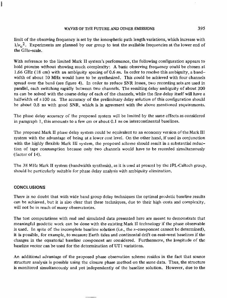
limit of the observing frequency is set by the ionospheric path length variations, which increase with l/vc2. Experiments are planned by our group to test the available frequencies at the lower end of the GHz-scale.

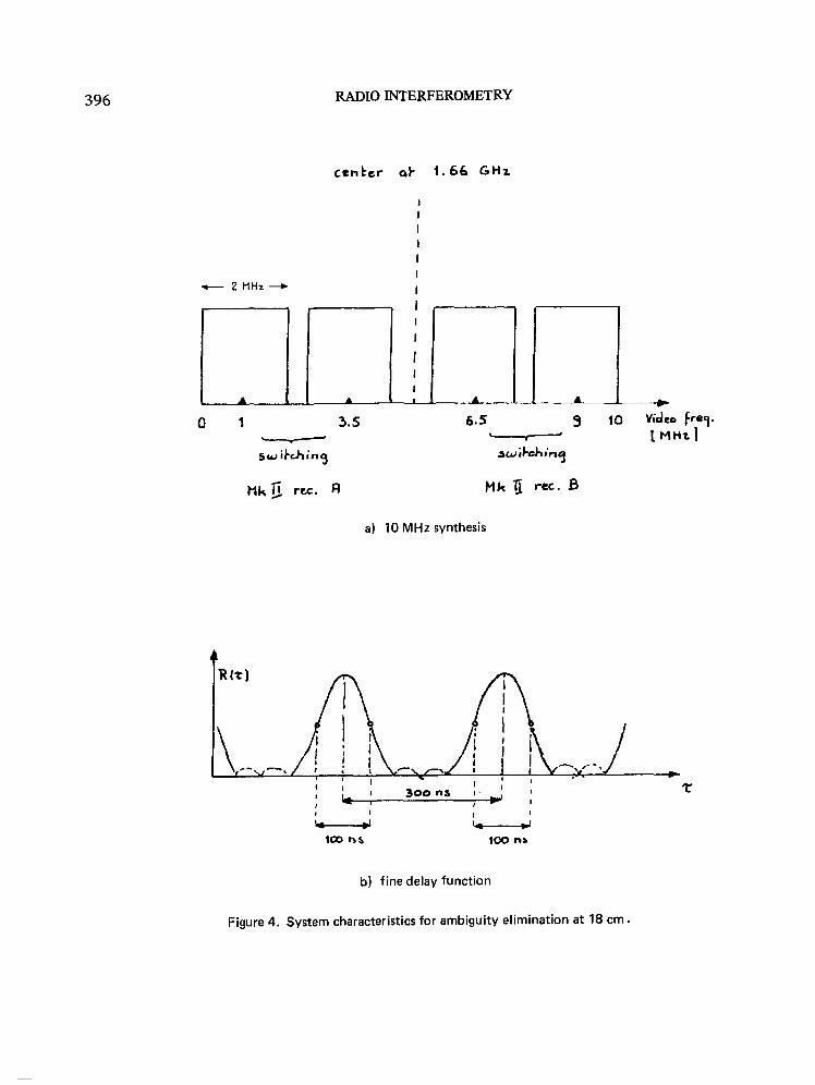
With reference to the limited Mark II system’s performance, the following configuration appears to hold promise without showing much complexity: A basic observing frequency could be chosen at 1.66 GHz (18 cm) with an ambiguity spacing of 0.6 ns. In order to resolve this ambiguity, a bandwidth of about 10 MHz would have to be synthesized. This could be achieved with four channels spread over the band (see figure 4). In order to reduce SNR losses, two recording sets are used in parallel, each switching rapidly between two channels. The resulting delay ambiguity of about 300 ns can be solved with the coarse delay of each of the channels, while the fine delay itself will have a halfwidth of + 100 ns. The accuracy of the preliminary delay solution of this configuration should be about 0.8 ns with good SNR, which is in agreement with the above mentioned requirements.

The phase delay accuracy of the proposed system will be limited by the same effects as considered in paragraph 1, this amounts to a few cm or about 0.1 ns on intercontinental baselines.

The proposed Mark II phase delay system could be equivalent to an economy version of the Mark III system with the advantage of being at a lower cost level. On the other hand, if used in conjunction with the highly flexible Mark III system, the proposed scheme should result in a substantial reduction of tape consumption because only two channels would have to be recorded simultaneously (factor of 14).

The 38 MHz Mark II system (bandwidth synthesis), as it is used at present by the JPL-Caltech group, should be particularly suitable for phase delay analysis with ambiguity elimination.

CONCLUSIONS

There is no doubt that with wide band group delay techniques the optimal geodetic baseline results can be achieved, but it is also clear that these techniques, due to their high costs and complexity, will not be in reach of many observatories.

The test computations with real and simulated data presented here are meant to demonstrate that meaningful geodetic work can be done with the existing Mark II technology if the phase observable is used. In spite of the incomplete baseline solution (i.e., the z-component cannot be determined), it is possible, for example, to measure Earth tides and continental drift on east-west baselines if the changes in the equatorial baseline component are considered. Furthermore, the longitude of the baseline vector can be used for the determination of UT 1 variations.

An additional advantage of the proposed phase observation scheme resides in the fact that source structure analysis is possible using the closure phase method on the same data. Thus, the structure is monitored simultaneously and yet independently of the baseline solution. However, due to the


0

a) 10 MHz synthesis

b) fine delay function

Figure 4. System characteristics for ambiguity elimination at 18 cm.


sensitivity of the pure phase solutions to instrumental and atmospheric effects, the full benefit of the high resolution of the phase observable can only be obtained if these effects are monitored with great care.

As an alternative, a system based on Mark II technology is outlined, which is capable of (a posteriori) resolving the phase ambiguities in order to achieve a complete baseline solution. With this system, it is possible to optimize observing strategies to obtain well conditioned baseline solutions that are less sensitive to long term instrumental and atmospheric effects.

REFERENCES

Moran, J. M.: Very Long Baseline Interferometric Observations and Data Reduction. Methods of Experimental Physics, Vol. 12, Part C, Radio Observations, Academic Press, New York, 1976.

Rogers, A. E. E. et al.: Geodesy by Radio Interferometry : Determination of a 1.24-km Baseline Vector with -5 mm Repeatability. J. Geophys. Res., Vol. 83, p. 325, 1978.

Shapiro, I. I., Wittels, J. J., et al.: Submilliarcsecond Astrometry via VLBI : I Relative Position of the Radio Sources 3C345 and NRA0 512. Preprint submitted to The Astronomical Journal April 1979.

Thomas, J. B.: An Analysis of Long Baseline Radio Interferometry. The Deep Space Network Pro- gress Report, Technical Report 32-1526, Vol. VII, VIII, XVI, Jet Propulsion Laboratory, Pasadena, Calif., 1972.

Whitney, A. R. et al.: A Very-Long-Baseline Interferometer System for Geodetic Applications. Radio Science, Vol. 11, p. 421-432, 1976.

Documents

PHASE VERSUS DELAY IN GEODETIC VLBI …...PHASE VERSUS DELAY IN GEODETIC VLBI James Campbell Geodetic Institute University of Bonn ABSTRACT For high precise baseline and source position