Embed Size (px)
Citation preview
Introduction to Survival Analysis
Sandra Taylor, Ph.D.
April 11 & 18, 2018
Seminar Objectives
Recognize survival data
Understand the unique aspects of survival data
Be able to generate and interpret survival curves
Learn how to compare two or more survival curves
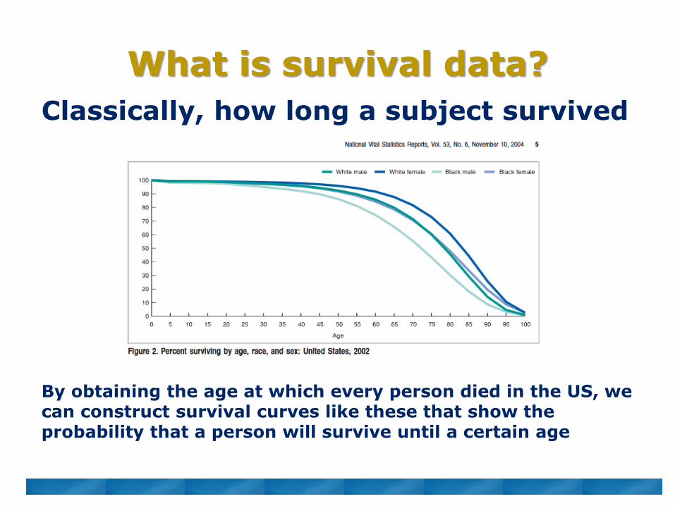
What is survival data?
Classically, how long a subject survived
By obtaining the age at which every person died in the US, we can construct survival curves like these that show the probability that a person will survive until a certain age
Time-to-Event Data
Bad Events – Death
– Recurrence of cancer
– Disease progression
– Failure of equipment
Good Events – Confirmed pregnancy
– Return to full function
– Completion of training
– Extubation
How does time-to-event data differ from other data types?
Consists of 2 pieces of information
– Time of observation (i.e., how long did you observe the subject)
– Outcome at the end of the observation period
Differs from other data types in having 2 components
– Consider cholesterol levels
– Consider presence of hypertension
What are challenges to analyzing time-to-event data?
Different observation lengths among subjects
Failure to observe the event of interest
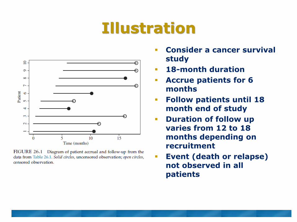
Illustration
Consider a cancer survival study
18-month duration
Accrue patients for 6 months
Follow patients until 18 month end of study
Duration of follow up varies from 12 to 18 months depending on recruitment
Event (death or relapse) not observed in all patients
Censoring
The survival time for a subject is “censored” if the event of interest is not observed.
Right censoring - event occurs after a specified time
Left censoring – event occurred before a specified time
Interval censoring – event known only to have occurred between to time points
Causes of Right Censoring
Administrative
– study designed to stop at a certain time
Withdrawal of patient from study
Loss to follow up
All handled the same way analytically
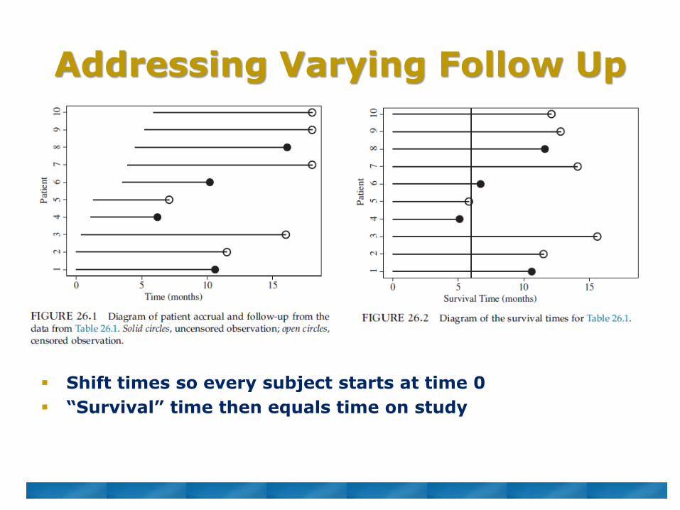
Addressing Varying Follow Up
Shift times so every subject starts at time 0
“Survival” time then equals time on study
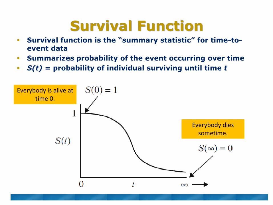
Survival Function Survival function is the “summary statistic” for time-to-
event data
Summarizes probability of the event occurring over time
S(t) = probability of individual surviving until time t
Everybody is alive at time 0.
Everybody dies sometime.
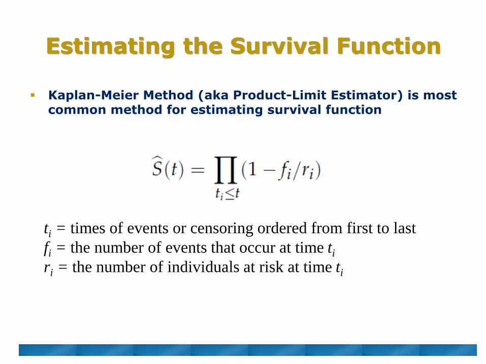
Estimating the Survival Function
Kaplan-Meier Method (aka Product-Limit Estimator) is most common method for estimating survival function
ti = times of events or censoring ordered from first to last
fi = the number of events that occur at time ti
ri = the number of individuals at risk at time ti
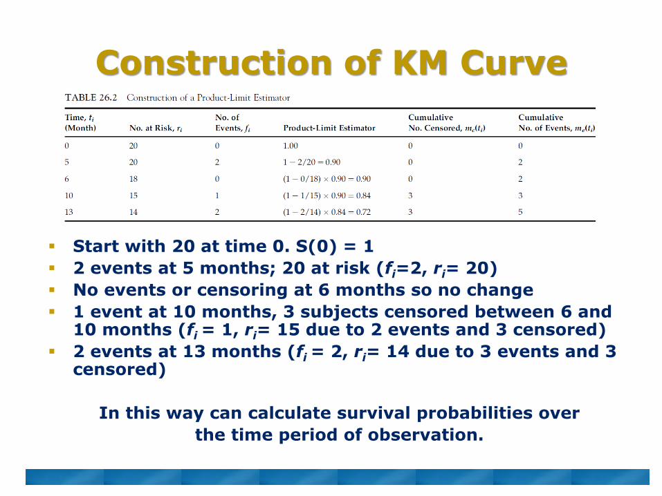
Construction of KM Curve
Start with 20 at time 0. S(0) = 1
2 events at 5 months; 20 at risk (fi=2, ri= 20)
No events or censoring at 6 months so no change
1 event at 10 months, 3 subjects censored between 6 and 10 months (fi = 1, ri= 15 due to 2 events and 3 censored)
2 events at 13 months (fi = 2, ri= 14 due to 3 events and 3 censored)
In this way can calculate survival probabilities over
the time period of observation.
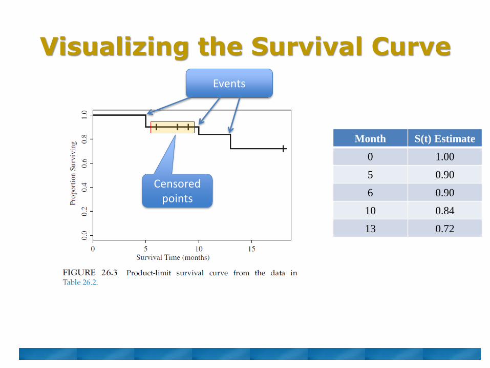
Visualizing the Survival Curve
Month S(t) Estimate
0 1.00
5 0.90
6 0.90
10 0.84
13 0.72
Censored points
Events
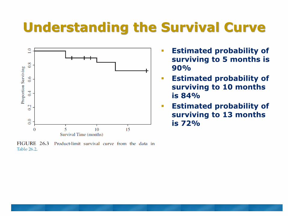
Understanding the Survival Curve
Estimated probability of surviving to 5 months is 90%
Estimated probability of surviving to 10 months is 84%
Estimated probability of surviving to 13 months is 72%
AIDS Clinical Trials Group Study
Double-blind trial that compared a 3 drug regimen to a 2 drug regimen
Eligible patients – CD4 counts < 200 and at least 3 months of prior zidovudine therapy
N = 1,151 subjects
Primary outcome: development of AIDS or death
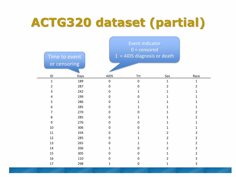
ACTG320 dataset (partial)
ID Days AIDS Trt Sex Race
1 189 0 0 1 1
2 287 0 0 2 2
3 242 0 1 1 1
4 199 0 0 1 1
5 286 0 1 1 1
6 285 0 1 1 1
7 270 0 0 1 2
8 285 0 1 1 2
9 276 0 0 1 1
10 306 0 0 1 1
11 334 0 1 2 3
12 285 0 1 2 2
13 265 0 1 1 2
14 206 1 0 2 2
15 305 0 0 1 2
16 110 0 0 2 3
17 298 1 0 1 3
Time to event or censoring
Event indicator 0 = censored
1 = AIDS diagnosis or death
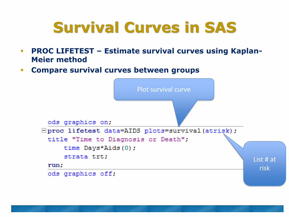
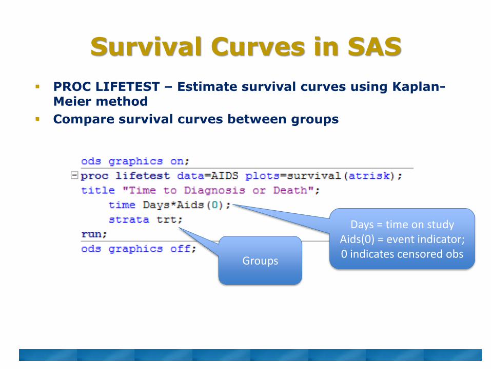
Survival Curves in SAS
PROC LIFETEST – Estimate survival curves using Kaplan-Meier method
Compare survival curves between groups
Plot survival curve
List # at risk
Survival Curves in SAS
PROC LIFETEST – Estimate survival curves using Kaplan-Meier method
Compare survival curves between groups
Groups
Days = time on study Aids(0) = event indicator; 0 indicates censored obs
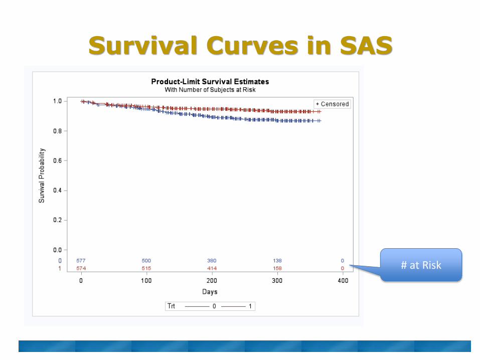
Survival Curves in SAS
# at Risk
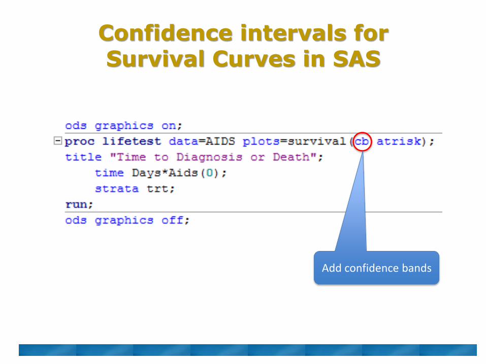
Confidence intervals for Survival Curves in SAS
Add confidence bands
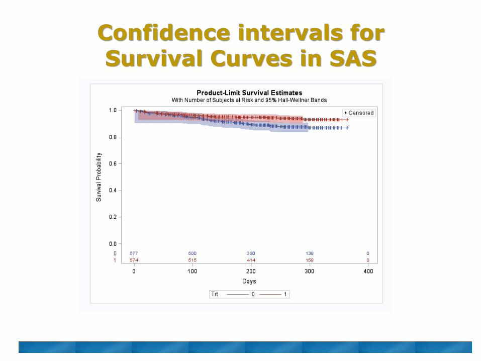
Confidence intervals for Survival Curves in SAS
Comparing Survival Curves
Ho: Survival curves do not differ between treatment groups
Here we have only two groups but method can be extended to more
Log-rank test is most common test
Other tests exist – differences stem from weights given to different portions of the survival curve
The Log-Rank Test
Determine expected number of events if no difference in survival
– expected number of events in each group is proportional to number at risk in each group
Compare observed to expected number of events
Marked deviation suggests survival curves differ between groups
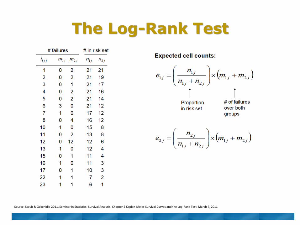
The Log-Rank Test
Source: Staub & Gekenidie 2011. Seminar in Statistics: Survival Analysis. Chapter 2 Kaplan-Meier Survival Curves and the Log-Rank Test. March 7, 2011
The Log-Rank Test
Source: Staub & Gekenidie 2011. Seminar in Statistics: Survival Analysis. Chapter 2 Kaplan-Meier Survival Curves and the Log-Rank Test. March 7, 2011
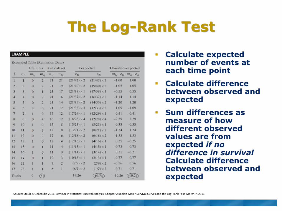
Calculate expected number of events at each time point
Calculate difference between observed and expected
Sum differences as measure of how different observed values are from expected if no difference in survival Calculate difference between observed and expected
The Log-Rank Test
Source: Staub & Gekenidie 2011. Seminar in Statistics: Survival Analysis. Chapter 2 Kaplan-Meier Survival Curves and the Log-Rank Test. March 7, 2011
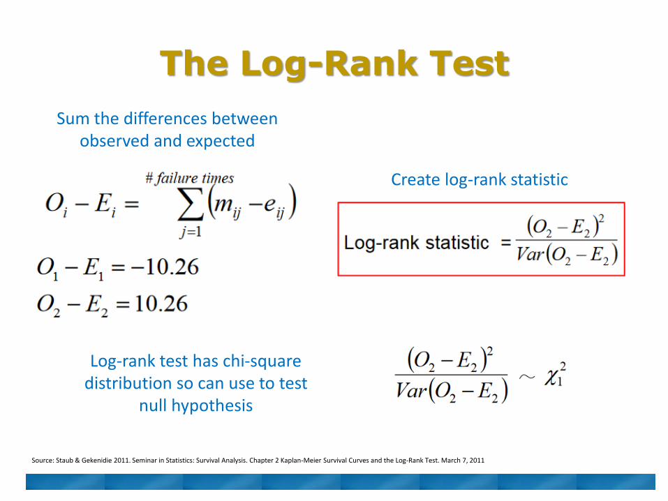
Sum the differences between observed and expected
Create log-rank statistic
Log-rank test has chi-square distribution so can use to test
null hypothesis
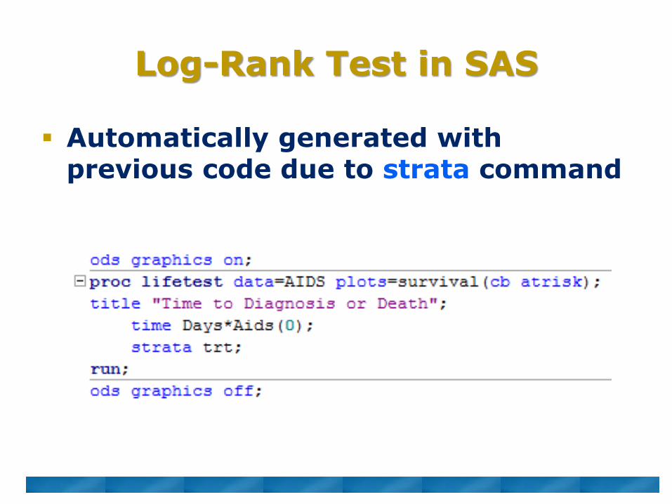
Log-Rank Test in SAS
Automatically generated with previous code due to strata command
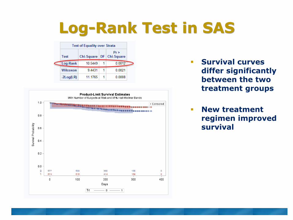
Log-Rank Test in SAS
Survival curves differ significantly between the two treatment groups
New treatment regimen improved survival
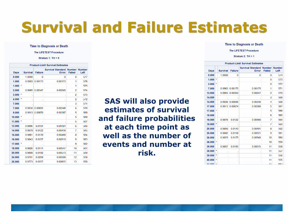
Survival and Failure Estimates
SAS will also provide estimates of survival
and failure probabilities at each time point as well as the number of events and number at
risk.
Another Example
Disease-free survival after bone marrow transplant
– Time to death or disease progression
3 risk categories
– ALL – acute lymphoblastic leukemia
– AML Low – Acute myeloctic leukemia
– AML High – Acute myeloctic leukemia
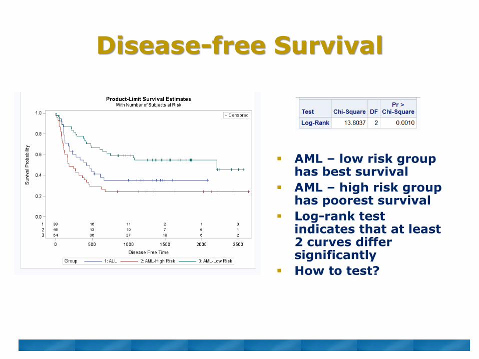
Disease-free Survival
AML – low risk group has best survival
AML – high risk group has poorest survival
Log-rank test indicates that at least 2 curves differ significantly
How to test?
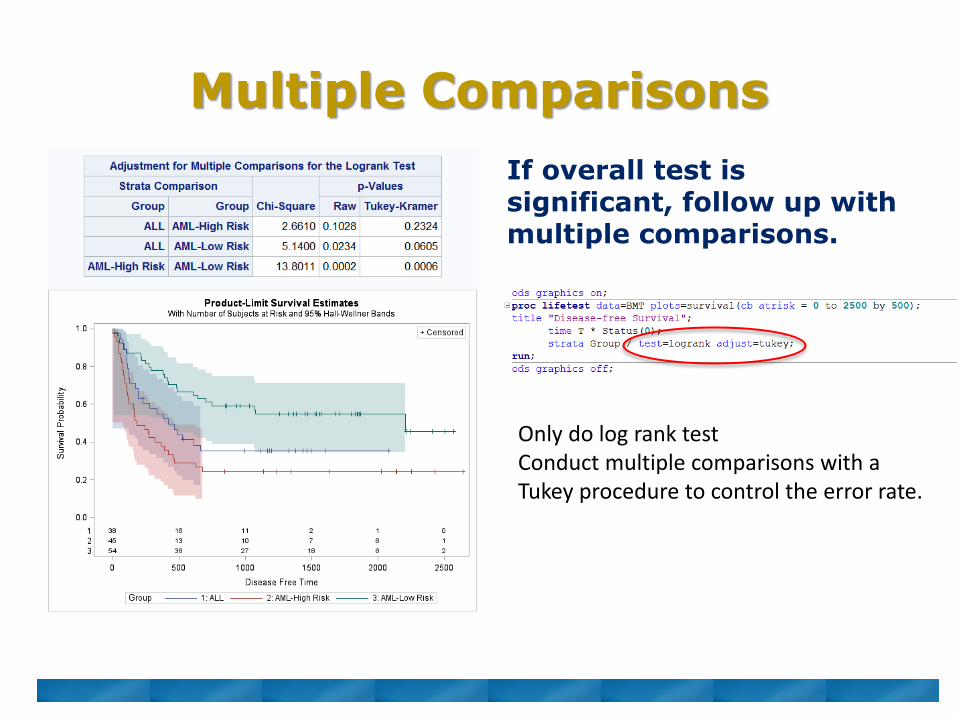
Multiple Comparisons
If overall test is significant, follow up with multiple comparisons.
Only do log rank test Conduct multiple comparisons with a Tukey procedure to control the error rate.
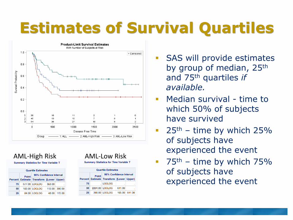
Estimates of Survival Quartiles
SAS will provide estimates by group of median, 25th and 75th quartiles if available.
Median survival - time to which 50% of subjects have survived
25th – time by which 25% of subjects have experienced the event
75th – time by which 75% of subjects have experienced the event
AML-High Risk AML-Low Risk
Summary
“Survival” analysis methods applicable to variety of “time-to-event” data
Censoring necessitates special methods
Kaplan-Meier summarizes survival data
Log-rank test statistically compares survival between categorical groups
Next month – regression analysis of survival data allowing evaluation of multiple categorical and continuous predictors
Help is Available
CTSC Biostatistics Office Hours
– Every Tuesday from 12 – 1:30 in Sacramento
– Sign-up through the CTSC Biostatistics Website
EHS Biostatistics Office Hours
– Every Monday from 2-4 in Davis
Request Biostatistics Consultations
– CTSC - www.ucdmc.ucdavis.edu/ctsc/
– EHS Center


![Visualizationmu = quartiles[1] sigma = 0.74*(quartiles[2]-quartiles[0]) print(mu, sigma) Aggregation & Grouping • Now we want to filter out all values that are more than away from](https://img.pdfslide.net/doc/110x75/60f899f38d692014c36763d5/visualization-mu-quartiles1-sigma-074quartiles2-quartiles0-printmu.jpg)