Investigation of Trajectory Optimization for Multiple …hh.diva-portal.org/smash/get/diva2:1072005/FULLTEXT01.pdf · Investigation of Trajectory Optimization for Multiple Car-Like

Investigation of Trajectory Optimization for MultipleCar-Like Vehicles

Semester Thesis

2015

Author: Pascal Fabian Bosshard

Supervisor: Dr. Roland Philippsen

Examiner: Prof. Dr. Roland Siegwart

School of Information Science, Computer and Electrical EngineeringHalmstad University

PO Box 823, SE-301 18 HALMSTADSweden

Investigation of Trajectory Optimization for Multiple Car-Like VehiclesPascal Fabian Bosshard

© Copyright Pascal Fabian Bosshard , 2015 . All rights reserved.Semester thesis reportSchool of Information Science, Computer and Electrical EngineeringCenter for Applied Intelligent System ResearchHalmstad University

Typset in 11pt Palatino (LATEX)

Contents

Abstract vii

Acknowledgments ix

Nomenclature xi

1 Introduction 11.1 Problem Setting and Goal of the Project . . . . . . . . . . . . . . . . . . . . 11.2 The Cargo-ANTs Project . . . . . . . . . . . . . . . . . . . . . . . . . . . . . 21.3 State-of-the-Art in Motion Planning and Trajectory Optimization . . . . . 31.4 Structure of the Report . . . . . . . . . . . . . . . . . . . . . . . . . . . . . . 3

2 Principle of CHOMP 52.1 Introduction . . . . . . . . . . . . . . . . . . . . . . . . . . . . . . . . . . . . 52.2 Functional Principle of CHOMP . . . . . . . . . . . . . . . . . . . . . . . . 6

3 Objective Functional Designs and Modeling 93.1 Introduction . . . . . . . . . . . . . . . . . . . . . . . . . . . . . . . . . . . . 93.2 The Objective Functional for a Planar Case . . . . . . . . . . . . . . . . . . 10

3.2.1 The Smoothness Objective . . . . . . . . . . . . . . . . . . . . . . . . 103.2.2 The Obstacle Objective . . . . . . . . . . . . . . . . . . . . . . . . . . 11

3.3 Objective Functional Designs . . . . . . . . . . . . . . . . . . . . . . . . . . 133.3.1 The Interference Objective . . . . . . . . . . . . . . . . . . . . . . . . 133.3.2 Curvature Constraints . . . . . . . . . . . . . . . . . . . . . . . . . . 16

4 Simulation Results 194.1 Introduction . . . . . . . . . . . . . . . . . . . . . . . . . . . . . . . . . . . . 194.2 Software Setup . . . . . . . . . . . . . . . . . . . . . . . . . . . . . . . . . . 194.3 Simulation Study . . . . . . . . . . . . . . . . . . . . . . . . . . . . . . . . . 20

4.3.1 Robot-to-Obstacle Performance . . . . . . . . . . . . . . . . . . . . . 214.3.2 Robot-to-Robot Performance . . . . . . . . . . . . . . . . . . . . . . 214.3.3 Curvature Insights . . . . . . . . . . . . . . . . . . . . . . . . . . . . 31

5 Conclusion and Future Work 335.1 Introduction . . . . . . . . . . . . . . . . . . . . . . . . . . . . . . . . . . . . 335.2 Evaluation of the Project . . . . . . . . . . . . . . . . . . . . . . . . . . . . . 335.3 Future Work . . . . . . . . . . . . . . . . . . . . . . . . . . . . . . . . . . . . 34

Appendix 35A Partial Derivatives for the 2D Curvature Representation . . . . . . . . . . . 35

i

List of Figures

1.1 Cargo-ANTs project illustration . . . . . . . . . . . . . . . . . . . . . . . . . 2

3.1 Extended overall objective functional . . . . . . . . . . . . . . . . . . . . . . 93.2 Plots of used cost functions . . . . . . . . . . . . . . . . . . . . . . . . . . . 133.3 Two intersecting trajectories and their connected points . . . . . . . . . . . 153.4 Unit vector representation for the interference objective . . . . . . . . . . . 153.5 Osculating circle of a robot’s position. . . . . . . . . . . . . . . . . . . . . . 16

4.1 The first and the final version of the GUI . . . . . . . . . . . . . . . . . . . . 204.2 Drawback using the unit vector approach for the interference objective . . 224.3 Interference objective comparison: Case 1 . . . . . . . . . . . . . . . . . . . 254.4 Interference objective comparison: Case 2 . . . . . . . . . . . . . . . . . . . 264.5 Interference objective comparison: Case 3 . . . . . . . . . . . . . . . . . . . 274.6 Interference objective comparison: Case 4 . . . . . . . . . . . . . . . . . . . 284.7 Interference objective comparison: Case 5 . . . . . . . . . . . . . . . . . . . 294.8 Interference objective comparison: Case 6 . . . . . . . . . . . . . . . . . . . 304.9 Illustration of the curvature . . . . . . . . . . . . . . . . . . . . . . . . . . . 32

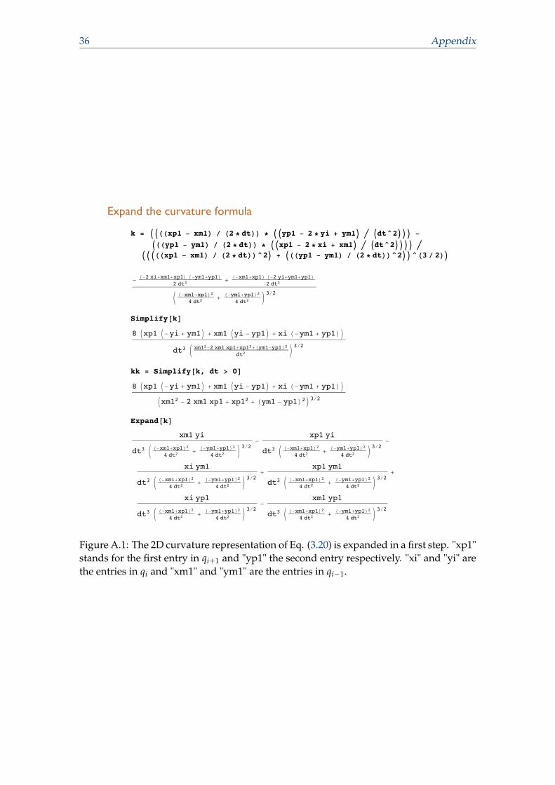
A.1 Expansion of the curvature formula . . . . . . . . . . . . . . . . . . . . . . 36A.2 Partial derivatives of the curvature . . . . . . . . . . . . . . . . . . . . . . . 37

iii

List of Tables

4.1 Parameter values . . . . . . . . . . . . . . . . . . . . . . . . . . . . . . . . . 214.2 Interference objective comparison: obstacle, starting and ending points

configurations . . . . . . . . . . . . . . . . . . . . . . . . . . . . . . . . . . . 23

v

Abstract

The purpose of the project at hand is to investigate a novel path- and trajectory- adapta-tion technique called CHOMP [13]. It is hoped that CHOMP simultaneously optimizesthe trajectory of multiple robots while obstacle avoidance of each robot should not beneglected. Furthermore, considering car-like steering constraints, the algorithm to be de-signed should take into account curvature to produce feasible paths.In a first step, a formulation of CHOMP for a 2D representation is obtained. Based onthis adaptation a graphical user interface and simulation tool is implemented. Addition-ally, two control strategies aiming at avoiding robot-robot collision are developed. Thefirst of these control algorithms is based on the usage of unit vectors for determiningthe geometric direction whereas the second relies on the usage of the obstacle avoidancefunctional. As a last step, various methods for incorporating curvature are explored, toinvestigate whether it is possible to directly integrate steering constraints into CHOMP.The performance of the adapted control algorithms is tested using simulation studies.It is found that the introduced methods for controlling the steering constraints are notable to optimize the trajectory in a satisfying way. However, CHOMP can be successfullyextended for a multiple robot scenario. Both obtained control strategies are feasible withslight differences in robustness and computational effort.

vii

Acknowledgments

My semester thesis at the Center for Applied Intelligent Systems Research (CAISR) pro-vided me with a deeper insight into robot motion planning and a great stay at a foreignuniversity. First of all I would like to thank my supervisor Dr. Roland Philippsen forenabling and supervising this project. His support and expertise in the field of roboticsallowed me to overcome numerous practical and theoretical issues. Additionally, I amvery thankful for his friendly initiation to the CAISR lab which turned my stay into anunforgettable time.I especially want to thank the PhD students Jennifer David and Saeed Gholami Shabandifor the inspiring discussions and practical help. Their knowledge in programming wereessential in order to implement the simulation program. I also want to thank the wholeCAISR members for their open-hearted integration into their lab.Finally, I would like to thank my tutor Prof. Dr. Roland Siegwart from ETH Zürich whomade my stay in Sweden possible.

Zürich, January 2015 Pascal Bosshard

ix

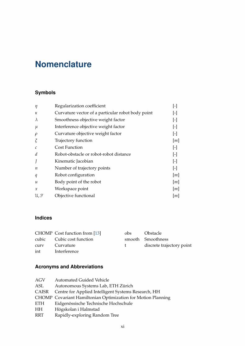
Nomenclature

Symbols

η Regularization coefficient [-]

κ Curvature vector of a particular robot body point [-]

λ Smoothness objective weight factor [-]

µ Interference objective weight factor [-]

ρ Curvature objective weight factor [-]

ξ Trajectory function [m]

c Cost Function [-]

d Robot-obstacle or robot-robot distance [-]

J Kinematic Jacobian [-]

n Number of trajectory points [-]

q Robot configuration [m]

u Body point of the robot [m]

x Workspace point [m]

U,F Objective functional [m]

Indices

CHOMP Cost function from [13]cubic Cubic cost functioncurv Curvatureint Interference

obs Obstaclesmooth Smoothnesst discrete trajectory point

Acronyms and Abbreviations

AGV Automated Guided VehicleASL Autonomous Systems Lab, ETH ZürichCAISR Centre for Applied Intelligent Systems Research, HHCHOMP Covariant Hamiltonian Optimization for Motion PlanningETH Eidgenössische Technische HochschuleHH Högskolan i HalmstadRRT Rapidly-exploring Random Tree

xi

Chapter 1

Introduction

1.1 Problem Setting and Goal of the Project

Nowadays, mobile robots are of great interest among different application sites like healthcare, transportation or the arms industry. They can on the one side support the user, onthe other side complete complex tasks independently. As Siegwart et al. in [10] demon-strates, a fully autonomous robot system has to deal with aspects like perception, local-ization, map building, cognition, path planning and motion control. Path planning is anessential part of it, with regard to obstacle avoidance, kinematic constraints and trajectoryoptimality. Various techniques exist which try to overcome these challenges. Neverthe-less, the difficulty of finding feasible solutions and the computational costs for multiplerobots systems are still among the most challenging tasks.The purpose of this project is to investigate a recent technique of trajectory optimization.In particular the CHOMP algorithm, presented by Zucker et al. [13], is used to designoptimal trajectories for multiple robots. It is hoped that this trajectory optimization tech-nique can be succesfully used for the given overall objective, see therefore section 1.2. Ina first step, the motion planning algorithm should lead to robust trajectories for a singlerobot in a 2D plane. After that, the algorithm should be extended to a multi-robot case.Beside considerations of robot-to-obstacle, also robot-to-robot distances are taken into ac-count at this moment. A main request is that it is possible to integrate this robot-to-robotbehaviour into CHOMP, retaining it therefore as a stand-alone algorithm. Furthermore,because of the nonholonomic constraints for two-steered-wheels robots and in some casesfor differential drive robots as well, their turning radius is limited. Paying regard to thetrajectory’s curvature, it is hoped that the algorithm simultaneously observes the radiuslimits. Hence the results would become optimal and smooth trajectories which are colli-sion free to obstacles and robots. And even the multi-robot case is explored in the 2D casefor this project, the resulting formulation would be able to support an arbitrary numberof dimensions.The semester thesis "Investigation of Trajectory Optimization for Multiple Car-Like Vehi-cles" is part of the Mechanical Engineering Master’s programme at Autonomous SystemsLab (ASL), ETH Zürich, Switzerland. It is carried out at Högskolan i Halmstad (HH) andembedded in the Mechatronics Group of the Centre for Applied Intelligent Systems Re-search (CAISR), HH, Sweden.The next two sections in this chapter explain in more detail why this project is carriedout. Section 1.2 gives an overview of the ongoing European project "Cargo-ANTs" andthe tasks of HH therein. Section 1.3 offers a short explanation of different motion plan-

1

2 Chapter 1. Introduction

ning and trajectory optimization techniques within the robotics community. Further-more, benefits and drawbacks of these state-of-the-art strategies are mentioned. Finally,an overview of this report is given in section 1.4.

1.2 The Cargo-ANTs Project

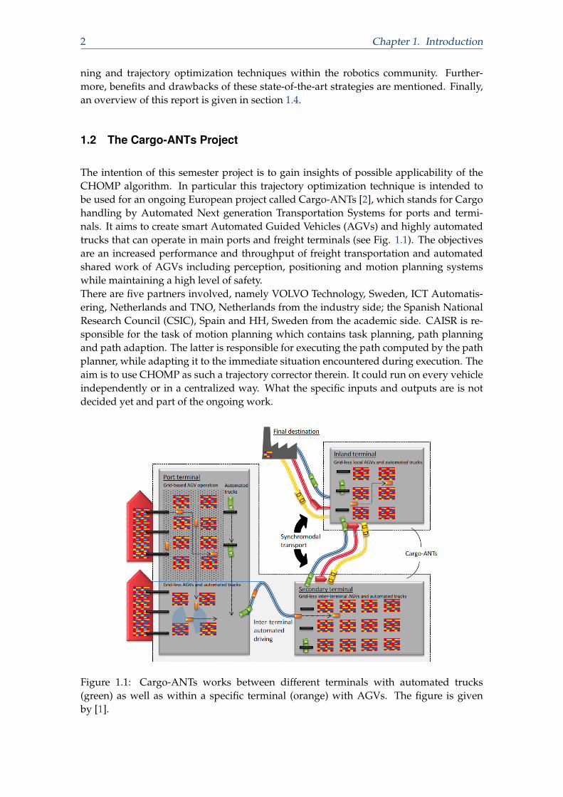
The intention of this semester project is to gain insights of possible applicability of theCHOMP algorithm. In particular this trajectory optimization technique is intended tobe used for an ongoing European project called Cargo-ANTs [2], which stands for Cargohandling by Automated Next generation Transportation Systems for ports and termi-nals. It aims to create smart Automated Guided Vehicles (AGVs) and highly automatedtrucks that can operate in main ports and freight terminals (see Fig. 1.1). The objectivesare an increased performance and throughput of freight transportation and automatedshared work of AGVs including perception, positioning and motion planning systemswhile maintaining a high level of safety.There are five partners involved, namely VOLVO Technology, Sweden, ICT Automatis-ering, Netherlands and TNO, Netherlands from the industry side; the Spanish NationalResearch Council (CSIC), Spain and HH, Sweden from the academic side. CAISR is re-sponsible for the task of motion planning which contains task planning, path planningand path adaption. The latter is responsible for executing the path computed by the pathplanner, while adapting it to the immediate situation encountered during execution. Theaim is to use CHOMP as such a trajectory corrector therein. It could run on every vehicleindependently or in a centralized way. What the specific inputs and outputs are is notdecided yet and part of the ongoing work.

Cargo-ANTs Cargo handling by Automated Next generation Transportation Systems for ports and terminals

RESEARCH PROJECT

PROJECT DESCRIPTION Cargo-ANTs aims to create smart Automated Guided Vehicles (AGVs) and Automated Trucks (ATs) that can co-operate in shared workspaces for efficient and safe freight transportation in main ports and freight terminals. The specific objectives are: 1. Increase performance and throughput of freight transportation in main ports and freight terminals and maintain a high level of safety. 2. Develop an automated shared work yard for smart AGVs and ATs. 3. Develop and demonstrate a robust grid-independent positioning system and an environmental perception system that oversees safety of operations. 4. Develop and demonstrate planning, decision, control and safety strategies for Automated Next generation Transportation systems (ANTs), i.e. smart AGVs and ATs.

KEY FIGURES: > Duration: Sept. 2013 to Sept. 2016 > Total budget: 4,7 Mill. € > Budget for IRI: 333 k€ (CSIC: 209k€ + UPC: 124k€)

www.iri.upc.edu

PROJECT PARTNERS: -  TNO, Netherlands -  Volvo Technology, Sweden -  ICT Automatisering, Netherlands -  CSIC, Spain (UPC as third party) -  Halmstad University, Sweden

IRI CONTACT: Dr. Juan Andrade Cetto [email protected]

RESEARCH QUESTIONS: -  Which combination of positioning techniques and sensors allow for reliable and

accurate positioning for the proposed applications? -  How can reliable environmental perception be achieved, in particular moving and

stationary object detection, drivable path detection, docking point detection, absolute and relative object positioning?

-  How to set up and integrate a vehicle control system, including high-level site planning, path planning, interaction planning, and feedback control?

-  How can functional safety of automated vehicles be achieved?

OUR CONTRIBUTIONS: -  Reliable vehicle localization -  Object detection and classification

Figure 1.1: Cargo-ANTs works between different terminals with automated trucks(green) as well as within a specific terminal (orange) with AGVs. The figure is givenby [1].

1.3. State-of-the-Art in Motion Planning and Trajectory Optimization 3

1.3 State-of-the-Art in Motion Planning and Trajectory Optimization

In the field of motion planning and trajectory optimization a lot of research has been donealready. Several approaches exist and the relationship to this work is listed below. Sincethe project is based on the application of [13] by Zucker et al., the author of this report hasnot undertaken a rigorous literature review. For more precise information, please refer toe.g. [13] or the references listed below.Sampling based motion planners have become well understood in the last years. Fur-thermore, it is recognised that randomization may not, by itself, account for their effi-ciency [6]. An often used method in the field of sampling based planners is Rapidly-exploring Random Trees (RRT) presented by LaValle [5]. It has been applied successfullyto differential constraints and high-dimensional planning, but still RRT and its extensionslack solution optimality and deterministic completeness, as stated in [10]. A recent ad-vance which overcomes this problem is RRT*, presented by Karaman and Frazzoli in [4].They introduce a new algorithm which is asymptotically optimal and show that the com-putational complexity is within a constant factor of the RRT counterpart.CHOMP does not lie on the approaches introduced above as it can be seen as a gradi-ent descent method. Zucker et al. in [13] distinguishes itself from other methods thatCHOMP assumes the availability of the gradient, instead of estimating the gradients us-ing sampling. Prior work in the field of functional gradient was done by Quinlan [9].The so-called elastic band method models the trajectory as a mass-spring system wheremotion planning is performed by scanning back and forth along the elastic while movingone point at the time. Similar to CHOMP, the internal forces try to minimize the distancebetween adjacent points which yields to a smooth trajectory. For example, Philippsenand Siegwart [8] show a successful implementation of elastic bands and other path plan-ning and obstacle avoidance methods.

1.4 Structure of the Report

The remaining chapters of this report are structured as follows: chapter 2 provides asummary of the main points in the investigated paper. It explains the general functionalprinciple and the advantages using this algorithm. Chapter 3 describes how the CHOMPobjective functionals are adapted for the project’s representation. Furthermore, chapter 3presents the new invented objective functional for multiple robots and an investigationof the trajectory’s curvature. In chapter 4 the software setup and the implemented GUIare presented. After that, chapter 4 contains the results of the derived overall objectivefunctional and the curvature study. Finally, chapter 5 draws a conclusion and gives anoutlook for future work in the field of motion planning and the CHOMP algorithm.

4 Chapter 1. Introduction

Chapter 2

Principle of CHOMP

2.1 Introduction

This chapter presents an overview of the CHOMP algorithm and conveys an understand-ing how this optimization technique works. The project’s achievements are based on thestructure of this algorithm, therefore the comprehension of it is essential.As given in the title of [13], CHOMP stands for Covariant Hamiltonian Optimization forMotion Planning. It is a trajectory optimization technique for motion planning in possiblehigh-dimensional spaces. The main goal is to produce optimal motion, i.e. finding theshortest possible way from a start to a goal point without violating dynamical constraints.To do so the algorithm deals with objective functionals which capture the dynamic of thetrajectory and avoidance of obstacles. A functional is a map from a vector space to itsfield of scalars, see also section 2.2. As mentioned before, CHOMP can be seen as a firstorder gradient descent method, searching therefore for local minima. The differences toalready existing gradient descent methods are explained by Zucker et al. in [13]. At thispoint it should be highlighted that CHOMP is a trajectory optimizer rather than a pathplanning algorithm. This implies two differences. First, it already needs a solution inthe beginning which connects the start point with the goal point. Second, CHOMP takestime into account. Therefore, CHOMP is capable of finding a valid trajectory even if it isstarted with an infeasible initial guess.Zucker et al. states two central tenets as requirements for his trajectory optimizationtechnique, which are displayed below:

• In [13] robot motion is stated as objective functionals. More precisely a smoothnessterm Usmooth[ξ] which captures the dynamic of the trajectory, and an obstacle termUobs[ξ] which provides the robot avoiding obstacles are formalized. The first teneton which CHOMP builds states that gradient information is often available andcan be computed inexpensively. Zucker et al. [13] first generalize the smoothnessfunctional in terms of a metric in the space of trajectories. Thereof they are ableto include higher-order derivatives. Furthermore, by using the robot’s workspaceinstead of the configuration space for the obstacle functional’s cost field c, they areable to compute functional gradients efficiently for complex real-world tasks.

• The second tenet aims for trajectories where the optimization is unencumbered bythe used parametrization. Invariance guarantees identical behaviour independentof the type of parametrization used. As explained in [13], a metric structure of thetrajectory space enables to precisely define perturbations of the trajectory. Using a

5

6 Chapter 2. Principle of CHOMP

functional and their gradient makes it covariant to reparametrization.

Built on these guidelines a variational method for optimization is used in [13]. As men-tioned above, a functional U[ξ] is a function of the trajectory function ξ. This function ξ

maps time t to robot configuration q for example. Finally the functional gradient ∇̄U[ξ]is the gradient of the functional U with respect to the trajectory ξ.

The presented trajectory optimization technique will descend to a local minimum. Tosample over a distribution of trajectories, [13] uses the Hamiltonian Monte Carlo algo-rithm. This method leverages gradient information to efficiently sample from a probabil-ity distribution p(ξ). At this point it has to be said that the sampling of trajectories is nota part of the project’s tasks. Therefore it will not be further considered in this report. Formore information please refer to chapter 5 in [13].The following section is intended to give an overview of the functional principle of theCHOMP algorithm. This will help to understand the solutions of the project tasks lateron.

2.2 Functional Principle of CHOMP

In order to obtain smooth and collision free trajectories, the objective functional measurestwo complementary aspects. These two terms Zucker et al. denotes in [13] as Fsmooth andFobs, and define together the objective functional:

U[ξ] = Fobs[ξ] + λFsmooth[ξ] (2.1)

where λ denotes a weight factor. As Eq. (2.1) shows, the objective is simply the weightedsum of a smoothness and an obstacle objective. As stated above, ξ maps time to robotconfiguration. The time is considered to range from 0 to 1 without loss of generality. Inthe following the two objectives are explained in more detail.To encourage smooth trajectories, unnecessary motion should be eliminated. Fsmooth mea-sures dynamical quantities such as velocity or acceleration across the trajectory. In [13],the smoothness objective is presented as follows:

Fsmooth[ξ] =12

∫ 1

0

∥∥∥∥ ddt

ξ(t)∥∥∥∥2

dt. (2.2)

The term inside the integral is the squared velocity norm and could also be replaced byother formulations. In this thesis, Eq. (2.2) will be directly used for deriving the simplifiedrepresentation and the implementation.The other objective introduced in (2.1) is the obstacle objective Fobs. It penalizes parts ofthe robot that are too close to obstacles or already in collision. As a result the consequenttrajectory is unencumbered by any obstacles. Zucker et al. defines Fobs in [13] as anintegral that gathers the cost encountered by each workspace body point on the robotacross the trajectory:

Fobs[ξ] =∫ 1

0

∫B

c ( x(ξ(t), u) )∥∥∥∥ d

dtx (ξ(t), u)

∥∥∥∥2

du dt. (2.3)

B denotes the set of points on the exterior robot’s body. c is the workspace cost functionwhich penalizes close obstacles. x(ξ(t), u) is defined as the forward kinematics, whichmaps a robot configuration q ∈ Q and a particular body point u ∈ B into the workspace.

2.2. Functional Principle of CHOMP 7

Through the multiplication of the cost function with the norm of the workspace velocity,Eq. (2.3) is transformed into an arc length parametrized line integral. This ensures thatthe obstacle objective is invariant to re-timing the trajectory.

As mentioned earlier, CHOMP uses a gradient method to optimize its trajectory. In thiscase the functional gradient ∇̄U is the perturbation φ : [0, 1] → C ⊂ Rd that maximizesU[ξ + εφ] as ε → 0, given in [13]. For a Euclidean norm and a differentiable objective ofthe form F[ξ] =

∫v(ξ(t))dt, the functional gradient is given as Quinlan developed in [9]:

∇̄F[ξ] = δvδξ− d

dtδvδξ ′

. (2.4)

Since the objective functional is the sum of the prior and the obstacle term, Eq. (2.1) caneasily be written for the functional gradient as

∇̄U = ∇̄Fobs + λ∇̄Fsmooth. (2.5)

Applying the definition of the functional gradient to the two objective terms (2.2) and(2.3), the result presented in [13] is:

∇̄Fsmooth[ξ](t) = −d2

dt2 ξ(t), (2.6)

∇̄Fobs[ξ] =∫B

JT ∥∥x′∥∥ [(I − x̂′ x̂′T)∇c− cκ] du, (2.7)

where κ =∥∥x′∥∥−2

(I − x̂′ x̂′T)x′′. (2.8)

J in Eq. (2.7) is the kinematic Jacobian at the particular body point. x′ and x′′ are thevelocity and acceleration of a body point and x̂′ is the normalized velocity vector. κ

denotes the curvature vector of a particular body point. Eq. (2.8) will be important againin section 3.3.2.

Given the gradient of U, it is possible to carry out gradient descent. In fact also a para-metrization of Fsmooth and Fobs is needed which depends on the given problem to solve.This is done in section 3.2. Zucker et al. [13] defines an iterative update rule that startsfrom an initial trajectory ξ0, for example a straight line between start and end point. Withthe actual trajectory ξi, a refined trajectory ξi+1 is then computed. The derivation of theupdate rule is done by solving the Lagrangian form of an optimization problem (seetherefore [13]). The resulting update rule is

ξi+1 = ξi −1η

A−1∇̄U[ξi]. (2.9)

η is a regularization coefficient which specifies the trade-off between step size and min-imizing U. Applying a steepest descent algorithm, unfortunately, gets dependent on thetrajectory’s representation. To get rid of this dependence on the parametrization the gra-dient ∇̄U is multiplied by the inverse matrix A. For the used representation later on, Ameasures the total amount of acceleration in the trajectory. A detailed derivation for theplanar case is given in section 3.2.1. In general, A is not related to the identically namedmatrix A in Eq. (3.9).Given the parametrization of the trajectory and differentiable objective functionals, it ispossible now to optimize the trajectory by using Eq. (2.9). At the end, a terminationcriteria may be used if the trajectory has to be fixed before execution. There are many

8 Chapter 2. Principle of CHOMP

possibilities, but a straightforward one is to terminate when the magnitude of ∇̄U[ξ] fallsbelow a predefined threshold. At this moment it is not sure if the encountered solutionis optimal in a global sense. With a higher-level planner one may decide if the trajectoryis kept or overruled, based on the quality and feasibility of the path.

Chapter 3

Objective Functional Designs and Modeling

3.1 Introduction

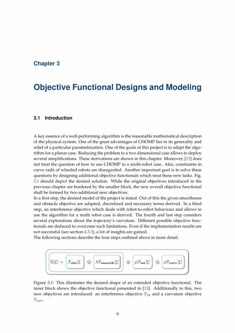
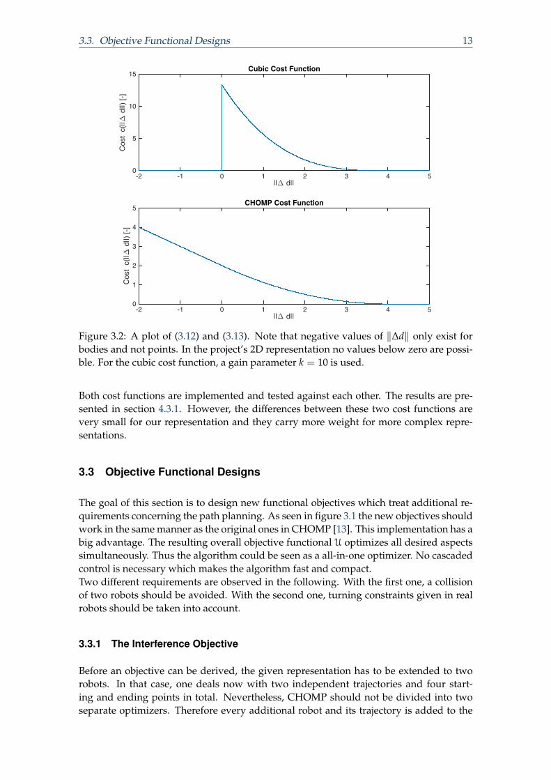
A key essence of a well-performing algorithm is the reasonable mathematical descriptionof the physical system. One of the great advantages of CHOMP lies in its generality andrelief of a particular parametrization. One of the goals of this project is to adapt the algo-rithm for a planar case. Reducing the problem to a two dimensional case allows to deployseveral simplifications. These derivations are shown in this chapter. Moreover, [13] doesnot treat the question of how to use CHOMP in a multi-robot case. Also, constraints incurve radii of wheeled robots are disregarded. Another important goal is to solve thesequestions by designing additional objective functionals which treat these new tasks. Fig.3.1 should depict the desired solution. While the original objectives introduced in theprevious chapter are bordered by the smaller block, the new overall objective functionalshall be formed by two additional new objectives.In a first step, the desired model of the project is stated. Out of this the given smoothnessand obstacle objective are adapted, discretized and necessary terms derived. In a thirdstep, an interference objective which deals with robot-to-robot behaviour and allows touse the algorithm for a multi robot case is derived. The fourth and last step considersseveral explorations about the trajectory’s curvature. Different possible objective func-tionals are deduced to overcome such limitations. Even if the implementation results arenot successful (see section 4.3.3), a lot of insights are gained.The following sections describe the four steps outlined above in more detail.

Fobs[⇠] �Fsmooth[⇠] µFint[⇠] ⇢Fcurv[⇠]U[⇠] =

Figure 3.1: This illustrates the desired shape of an extended objective functional. Theinner block shows the objective functional presented in [13]. Additionally to this, twonew objectives are introduced: an interference objective Fint and a curvature objectiveFcurv.

9

10 Chapter 3. Objective Functional Designs and Modeling

3.2 The Objective Functional for a Planar Case

As this project serves as a first investigation for the use of CHOMP in the Cargo-ANTsproject, the representation can be relatively simple. A reasonable possibility is to con-sider a point robot which moves freely in a 2D plane. This simplifies various things likeclearer equations, easier implementation of a trajectory representation and shorter run-time. Nevertheless, it is still a good approximation to the encountered situation in theCargo-ANTs project.

Before the two objective terms Fsmooth and Fobs are derived for the desired robot represen-tation, a particular parametrization of the trajectory ξ has to be chosen. For this case, thesame like in [13] is used. A uniform discretization samples the trajectory function overequal time steps of length ∆t:

ξ ≈ (q1, q2, ..., qn)T (3.1)

Each robot configuration qi represents a point in the discretized trajectory and containsby itself an x- and y-coordinate, ~qi = (xi

yi). As already done before, the vector arrow

is eschewed for the sake of simplicity. Furthermore it is assumed that the starting andending points are fixed, given as q0 and qn+1 respectively.

3.2.1 The Smoothness Objective

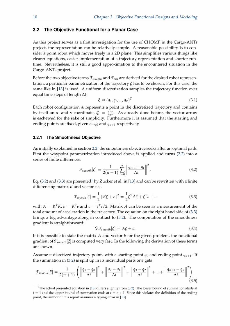
As initially explained in section 2.2, the smoothness objective seeks after an optimal path.First the waypoint parametrization introduced above is applied and turns (2.2) into aseries of finite differences:

Fsmooth[ξ] =1

2(n + 1)

n

∑t=0

∥∥∥∥qt+1 − qt

∆t

∥∥∥∥2

. (3.2)

Eq. (3.2) and (3.3) are presented1 by Zucker et al. in [13] and can be rewritten with a finitedifferencing matrix K and vector e as

Fsmooth[ξ] =12‖Kξ + e‖2 =

12

ξTAξ + ξTb + c (3.3)

with A = KTK, b = KTe and c = eTe/2. Matrix A can be seen as a measurement of thetotal amount of acceleration in the trajectory. The equation on the right hand side of (3.3)brings a big advantage along in contrast to (3.2). The computation of the smoothnessgradient is straightforward:

∇̄Fsmooth[ξ] = Aξ + b. (3.4)

If it is possible to state the matrix A and vector b for the given problem, the functionalgradient of Fsmooth[ξ] is computed very fast. In the following the derivation of these termsare shown.

Assume n disretized trajectory points with a starting point q0 and ending point qn+1. Ifthe summation in (3.2) is split up in its individual parts one gets

Fsmooth[ξ] =1

2(n + 1)

(∥∥∥∥q1 − q0

∆t

∥∥∥∥2

+

∥∥∥∥q2 − q1

∆t

∥∥∥∥2

+

∥∥∥∥q3 − q2

∆t

∥∥∥∥2

+ ... +∥∥∥∥qn+1 − qn

∆t

∥∥∥∥2)

.

(3.5)1The actual presented equation in [13] differs slightly from (3.2). The lower bound of summation starts at

t = 1 and the upper bound of summation ends at t = n + 1. Since this violates the definition of the endingpoint, the author of this report assumes a typing error in [13].

3.2. The Objective Functional for a Planar Case 11

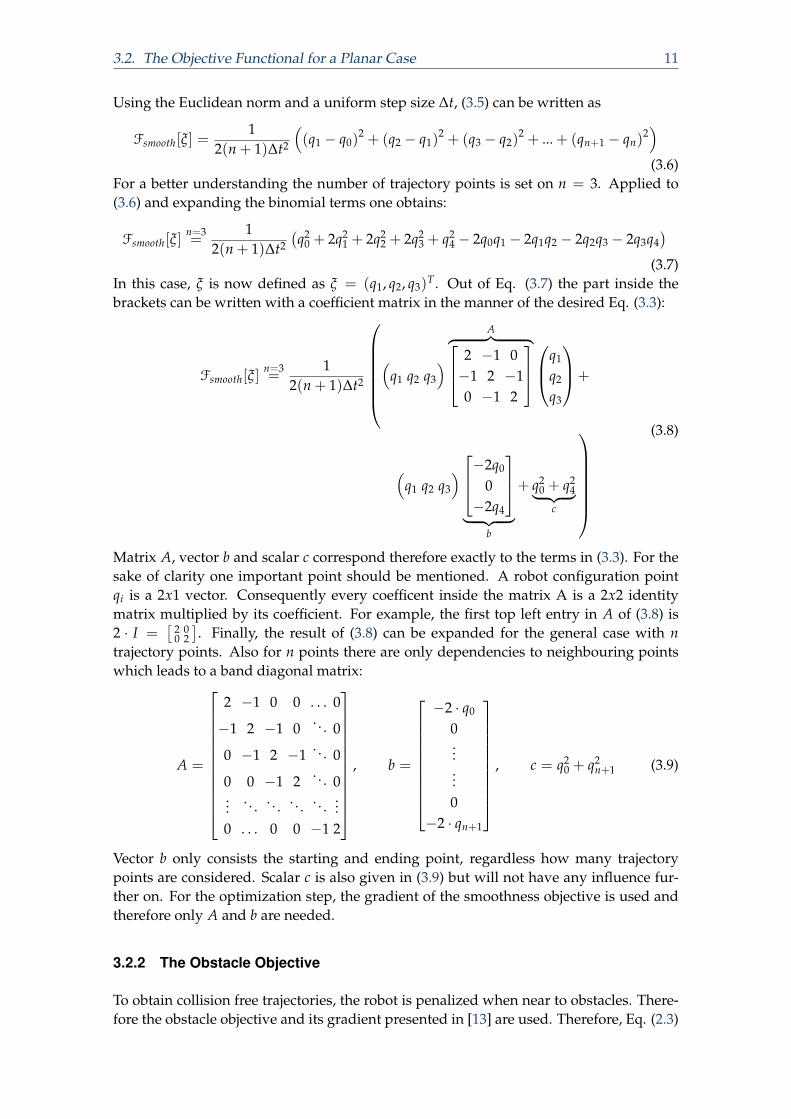
Using the Euclidean norm and a uniform step size ∆t, (3.5) can be written as

Fsmooth[ξ] =1

2(n + 1)∆t2

((q1 − q0)

2 + (q2 − q1)2 + (q3 − q2)

2 + ... + (qn+1 − qn)2)(3.6)

For a better understanding the number of trajectory points is set on n = 3. Applied to(3.6) and expanding the binomial terms one obtains:

Fsmooth[ξ]n=3=

12(n + 1)∆t2

(q2

0 + 2q21 + 2q2

2 + 2q23 + q2

4 − 2q0q1 − 2q1q2 − 2q2q3 − 2q3q4)

(3.7)In this case, ξ is now defined as ξ = (q1, q2, q3)T. Out of Eq. (3.7) the part inside thebrackets can be written with a coefficient matrix in the manner of the desired Eq. (3.3):

Fsmooth[ξ]n=3=

12(n + 1)∆t2

(

q1 q2 q3

)A︷︸︸︷ 2 −1 0

−1 2 −10 −1 2

q1

q2

q3

+

(q1 q2 q3

) −2q0

0−2q4

︸︷︷︸

b

+ q20 + q2

4︸︷︷︸c

(3.8)

Matrix A, vector b and scalar c correspond therefore exactly to the terms in (3.3). For thesake of clarity one important point should be mentioned. A robot configuration pointqi is a 2x1 vector. Consequently every coefficent inside the matrix A is a 2x2 identitymatrix multiplied by its coefficient. For example, the first top left entry in A of (3.8) is2 · I =

[2 00 2

]. Finally, the result of (3.8) can be expanded for the general case with n

trajectory points. Also for n points there are only dependencies to neighbouring pointswhich leads to a band diagonal matrix:

A =

2 −1 0 0 . . . 0

−1 2 −1 0. . . 0

0 −1 2 −1. . . 0

0 0 −1 2. . . 0

.... . . . . . . . . . . .

...0 . . . 0 0 −1 2

, b =

−2 · q0

0......0

−2 · qn+1

, c = q2

0 + q2n+1 (3.9)

Vector b only consists the starting and ending point, regardless how many trajectorypoints are considered. Scalar c is also given in (3.9) but will not have any influence fur-ther on. For the optimization step, the gradient of the smoothness objective is used andtherefore only A and b are needed.

3.2.2 The Obstacle Objective

To obtain collision free trajectories, the robot is penalized when near to obstacles. There-fore the obstacle objective and its gradient presented in [13] are used. Therefore, Eq. (2.3)


only has to be slightly modified to be used for the project’s desired manner. Since onlya point robot is considered, the workspace body point x(ξ(t), u) simplifies to x(ξ(t). Inaddition, the configuration space and the workspace are the same. This makes it possibleto define x ≡ q. Using the same discretized waypoint parametrization as for Fsmooth[ξ],the gradient of the obstacle objective derived from (2.7) is

∇̄Fobs[ξ] =n

∑t=0

JT∥∥∥∥qt+1 − qt

∆t

∥∥∥∥ [(I − v̂v̂T)∇c− cκ], where v̂ =qt+1−qt

∆t∥∥∥ qt+1−qt∆t

∥∥∥ . (3.10)

The Jacobian maps the projection between configuration and geometrical space. In ourrepresentation this is the same and therefore the Jacobian is equal to the identity matrix,J ≡ I. The curvature vector (2.8) can be written as:

κ =

∥∥∥∥qt+1 − qt

∆t

∥∥∥∥−2 (I − v̂v̂T

)· ∇̄Fsmooth. (3.11)

In this case, the acceleration x′′ is equal to the gradient of the smoothness objective. Thismakes sense because ∇̄Fsmooth is defined in (2.6) as the second derivative of ξ.

Cost Function Variations

For applying Eq. (3.10) a cost function c which penalizes the robot for being near obstaclesis also needed. Given a trajectory through space, the cost is defined by the distancebetween the robot’s body and the obstacles. A trajectory ξ is collision-free if for everyconfiguration qi ∈ ξ the distances from the robot to any obstacles are greater than somethreshold ε > 0. Beside of that, Zucker et al. [13] determines a distance field where alldistances from any point in the workspace to the surface of obstacles are mapped. Forthe implementation of the simplified 2D representation the obstacles are assumed to becircles with known radii. The cost function depends therefore on the Euclidean distancesbetween every trajectory point and the center of the obstacles.

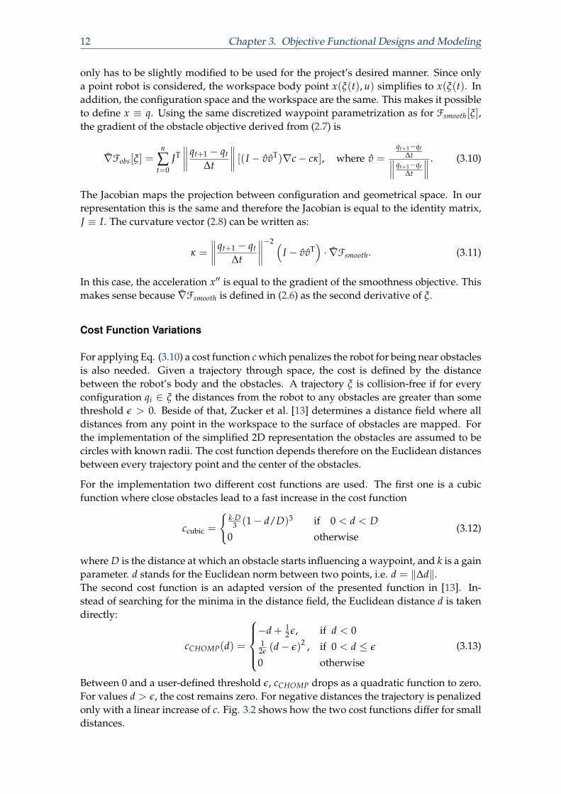
For the implementation two different cost functions are used. The first one is a cubicfunction where close obstacles lead to a fast increase in the cost function

ccubic =

{k·D

3 (1− d/D)3 if 0 < d < D

0 otherwise(3.12)

where D is the distance at which an obstacle starts influencing a waypoint, and k is a gainparameter. d stands for the Euclidean norm between two points, i.e. d = ‖∆d‖.The second cost function is an adapted version of the presented function in [13]. In-stead of searching for the minima in the distance field, the Euclidean distance d is takendirectly:

cCHOMP(d) =

−d + 1

2 ε, if d < 012ε (d− ε)2 , if 0 < d ≤ ε

0 otherwise

(3.13)

Between 0 and a user-defined threshold ε, cCHOMP drops as a quadratic function to zero.For values d > ε, the cost remains zero. For negative distances the trajectory is penalizedonly with a linear increase of c. Fig. 3.2 shows how the two cost functions differ for smalldistances.

3.3. Objective Functional Designs 13

||" d||-2 -1 0 1 2 3 4 5

Cos

t c(

||" d

||) [-

]

0

5

10

15Cubic Cost Function

||" d||-2 -1 0 1 2 3 4 5

Cos

t c(

||" d

||) [-

]

0

1

2

3

4

5CHOMP Cost Function

Figure 3.2: A plot of (3.12) and (3.13). Note that negative values of ‖∆d‖ only exist forbodies and not points. In the project’s 2D representation no values below zero are possi-ble. For the cubic cost function, a gain parameter k = 10 is used.

Both cost functions are implemented and tested against each other. The results are pre-sented in section 4.3.1. However, the differences between these two cost functions arevery small for our representation and they carry more weight for more complex repre-sentations.

3.3 Objective Functional Designs

The goal of this section is to design new functional objectives which treat additional re-quirements concerning the path planning. As seen in figure 3.1 the new objectives shouldwork in the same manner as the original ones in CHOMP [13]. This implementation has abig advantage. The resulting overall objective functional U optimizes all desired aspectssimultaneously. Thus the algorithm could be seen as a all-in-one optimizer. No cascadedcontrol is necessary which makes the algorithm fast and compact.Two different requirements are observed in the following. With the first one, a collisionof two robots should be avoided. With the second one, turning constraints given in realrobots should be taken into account.

3.3.1 The Interference Objective

Before an objective can be derived, the given representation has to be extended to tworobots. In that case, one deals now with two independent trajectories and four start-ing and ending points in total. Nevertheless, CHOMP should not be divided into twoseparate optimizers. Therefore every additional robot and its trajectory is added to the


existing trajectory:ξ = (q1, q2, ..., qn, qn+3, qn+4, ..., q2n+2)

T. (3.14)

Eq. (3.14) is valid when two robots are considered which have the starting points q0, qn+2

and the ending points qn+1, q2n+3. Obviously the matrix A, vector b and scalar c of (3.9)change when ξ gets bigger. For the assumption that the trajectories of both robots containthe same quantity of points, A and b can be stacked:

A2R =

[A 00 A

]=

2 −1 0 . . . 0 0 . . . 0

−1 2 −1. . . 0 0

...

0 −1 2. . .

.... . .

......

. . . . . . . . . 0 . . . 00 0 . . . 0 2 −1 0 . . .

0 0... −1 2 −1

. . ....

. . .... 0 −1 2

. . .

0 . . . 0...

. . . . . . . . .

, b2R =

−2 · q0

0...0

−2 · qn+1

−2 · qn+2

0...0

−2 · q2n+3

, (3.15)

c2R = q20 + q2

n+1 + q2n+2 + q2

n+3.

If more than two robots are treated, then the terms in (3.15) are enlarged in the same way.The change from one to two robots doesn’t change a lot in the implementation. The mostadjustments have to be done in the adaption of the GUI to display all trajectory pointscorrectly (see also section 4.2).

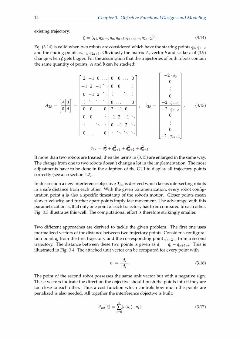
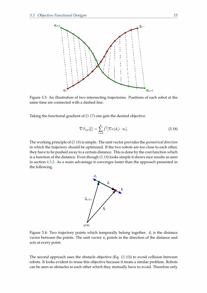
In this section a new interference objective Fint is derived which keeps intersecting robotsin a safe distance from each other. With the given parametrization, every robot config-uration point q is also a specific timestamp of the robot’s motion. Closer points meanslower velocity, and further apart points imply fast movement. The advantage with thisparametrization is, that only one point of each trajectory has to be compared to each other.Fig. 3.3 illustrates this well. The computational effort is therefore strikingly smaller.

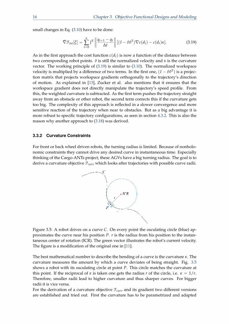
Two different approaches are derived to tackle the given problem. The first one usesmormalized vectors of the distance between two trajectory points. Consider a configura-tion point qi from the first trajectory and the corresponding point qn+2+i from a secondtrajectory. The distance between these two points is given as di = qi − qn+2+i. This isillustrated in Fig. 3.4. The attached unit vector can be computed for every point with

ni =di

‖di‖. (3.16)

The point of the second robot possesses the same unit vector but with a negative sign.These vectors indicate the direction the objective should push the points into if they aretoo close to each other. Thus a cost function which controls how much the points arepenalized is also needed. All together the interference objective is built:

Fint[ξ] =n

∑t=0

[c(di) · nt]. (3.17)


Figure 3.3: An illustration of two intersecting trajectories. Positions of each robot at thesame time are connected with a dashed line.

Taking the functional gradient of (3.17) one gets the desired objective:

∇̄Fint[ξ] =n

∑t=0

JT[∇c(di) · nt]. (3.18)

The working principle of (3.18) is simple. The unit vector provides the geometrical directionin which the trajectory should be optimized. If the two robots are too close to each other,they have to be pushed away to a certain distance. This is done by the cost function whichis a function of the distance. Even though (3.18) looks simple it shows nice results as seenin section 4.3.2. As a main advantage it converges faster than the approach presented inthe following.

Figure 3.4: Two trajectory points which temporally belong together. di is the distancevector between the points. The unit vector ni points in the direction of the distance andacts at every point.

The second approach uses the obstacle objective (Eq. (3.10)) to avoid collision betweenrobots. It looks evident to reuse this objective because it treats a similar problem. Robotscan be seen as obstacles to each other which they mutually have to avoid. Therefore only


small changes in Eq. (3.10) have to be done:

∇̄Fint[ξ] =n

∑t=0

JT∥∥∥∥qt+1 − qt

∆t

∥∥∥∥ [(I − v̂v̂T)∇c(dt)− c(dt)κ]. (3.19)

As in the first approach the cost function c(dt) is now a function of the distance betweentwo corresponding robot points. v̂ is still the normalized velocity and κ is the curvaturevector. The working principle of (3.19) is similar to (3.10). The normalized workspacevelocity is multiplied by a difference of two terms. In the first one, (I − v̂v̂T) is a projec-tion matrix that projects workspace gradients orthogonally to the trajectory’s directionof motion. As explained in [13], Zucker et al. also mentions that it ensures that theworkspace gradient does not directly manipulate the trajectory’s speed profile. Fromthis, the weighted curvature is subtracted. As the first term pushes the trajectory straightaway from an obstacle or other robot, the second term corrects this if the curvature getstoo big. The complexity of this approach is reflected in a slower convergence and moresensitive reaction of the trajectory when near to obstacles. But as a big advantage it ismore robust to specific trajectory configurations, as seen in section 4.3.2. This is also thereason why another approach to (3.18) was derived.

3.3.2 Curvature Constraints

For front or back wheel driven robots, the turning radius is limited. Because of nonholo-nomic constraints they cannot drive any desired curve in instantaneous time. Especiallythinking of the Cargo-ANTs project, these AGVs have a big turning radius. The goal is toderive a curvature objective Fcurv which looks after trajectories with possible curve radii.

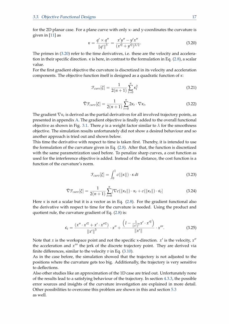
Figure 3.5: A robot drives on a curve C. On every point the osculating circle (blue) ap-proximates the curve near his position P. r is the radius from his position to the instan-taneous center of rotation (ICR). The green vector illustrates the robot’s current velocity.The figure is a modification of the original one in [11].

The best mathematical number to describe the bending of a curve is the curvature κ. Thecurvature measures the amount by which a curve deviates of being straight. Fig. 3.5shows a robot with its osculating circle at point P. This circle matches the curvature atthis point. If the reciprocal of κ is taken one gets the radius r of the circle, i.e. κ = 1/r.Therefore, smaller radii lead to higher curvature and thus sharper curves. For biggerradii it is vice versa.For the derivation of a curvature objective Fcurv and its gradient two different versionsare established and tried out. First the curvature has to be parametrized and adapted


for the 2D planar case. For a plane curve with only x- and y-coordinates the curvature isgiven in [11] as

κ =q′ × q′′

‖q′‖3 =x′y′′ − y′x′′

(x′2 + y′2)3/2 . (3.20)

The primes in (3.20) refer to the time derivatives, i.e. these are the velocity and accelera-tion in their specific direction. κ is here, in contrast to the formulation in Eq. (2.8), a scalarvalue.For the first gradient objective the curvature is discretized in its velocity and accelerationcomponents. The objective function itself is designed as a quadratic function of κ:

Fcurv[ξ] =1

2(n + 1)

n

∑t=0

κ2t (3.21)

∇̄Fcurv[ξ] =1

2(n + 1)

n

∑t=0

2κt · ∇κt. (3.22)

The gradient∇κt is derived as the partial derivatives for all involved trajectory points, aspresented in appendix A. The gradient objective is finally added to the overall functionalobjective as shown in Fig. 3.1. There ρ is a weight factor similar to λ for the smoothnessobjective. The simulation results unfortunately did not show a desired behaviour and soanother approach is tried out and shown below.This time the derivative with respect to time is taken first. Thereby, it is intended to usethe formulation of the curvature given in Eq. (2.8). After that, the function is discretizedwith the same parametrization used before. To penalize sharp curves, a cost function asused for the interference objective is added. Instead of the distance, the cost function is afunction of the curvature’s norm.

Fcurv[ξ] =∫ 1

0c(‖κ‖) · κ dt (3.23)

∇̄Fcurv[ξ] =1

2(n + 1)

n

∑t=0

[∇c(‖κt‖) · κt + c(‖κt‖) · κ̇t] (3.24)

Here κ is not a scalar but it is a vector as in Eq. (2.8). For the gradient functional alsothe derivative with respect to time for the curvature is needed. Using the product andquotient rule, the curvature gradient of Eq. (2.8) is:

κ̇t =(x′′ · x′T + x′ · x′′T)

‖x′‖3 · x′′ +

(I − 1

‖x′‖2 x′ · x′T)

‖x′‖ · x′′′. (3.25)

Note that x is the workspace point and not the specific x-direction. x′ is the velocity, x′′

the acceleration and x′′′ the jerk of the discrete trajectory point. They are derived viafinite differences, similar to the velocity v in Eq. (3.10).As in the case before, the simulation showed that the trajectory is not adjusted to thepositions where the curvature gets too big. Additionally, the trajectory is very sensitiveto deflections.Also other studies like an approximation of the 1D case are tried out. Unfortunately noneof the results lead to a satisfying behaviour of the trajectory. In section 4.3.3, the possibleerror sources and insights of the curvature investigation are explained in more detail.Other possibilities to overcome this problem are shown in this and section 5.3as well.


Chapter 4

Simulation Results

4.1 Introduction

In order to better understand the way CHOMP works, a graphical representation is use-ful. While numbers are hard to transfer into a physical meaning, a graphical user inter-face (GUI) directly shows solutions or problems. This chapter shows the derived GUI forthe stated project’s model and the simulation results tested on it.Section 4.2 explains how the graphical representation is built and how it can be used.As the standard CHOMP algorithm had been extended, the GUI was also customized toillustrate the new features. The progress in this is also shown. In section 4.3 results of thenew functional objectives are discussed. This contains for one thing the obstacle objec-tive with its different cost functions, for another thing the two robot-to-robot behaviourapproaches. Finally, the takeaways from the curvature study are presented.

4.2 Software Setup

The GUI has three main tasks to solve. First, it should deliver a graphical answer of howthe algorithm works. Second, the robustness of the derived approaches should be com-parable. And at last, it should serve as a platform to experiment with different scenarios.At the beginning of this project a simple GUI was already available, programmed by thesupervisor of this project. The GUI is coded in C++ and platform independent. A goodreference which the author of this text also used to get familiar with the programme lan-guage is given by Arnold Willemer [12]. For the implementation, for one thing Eigen [3]is used, a C++ template library for linear algebra which makes it more user-friendly todeal with matrices and vectors. For another thing, GTK+ [7] is used, which is needed tocreate the graphical user interface.

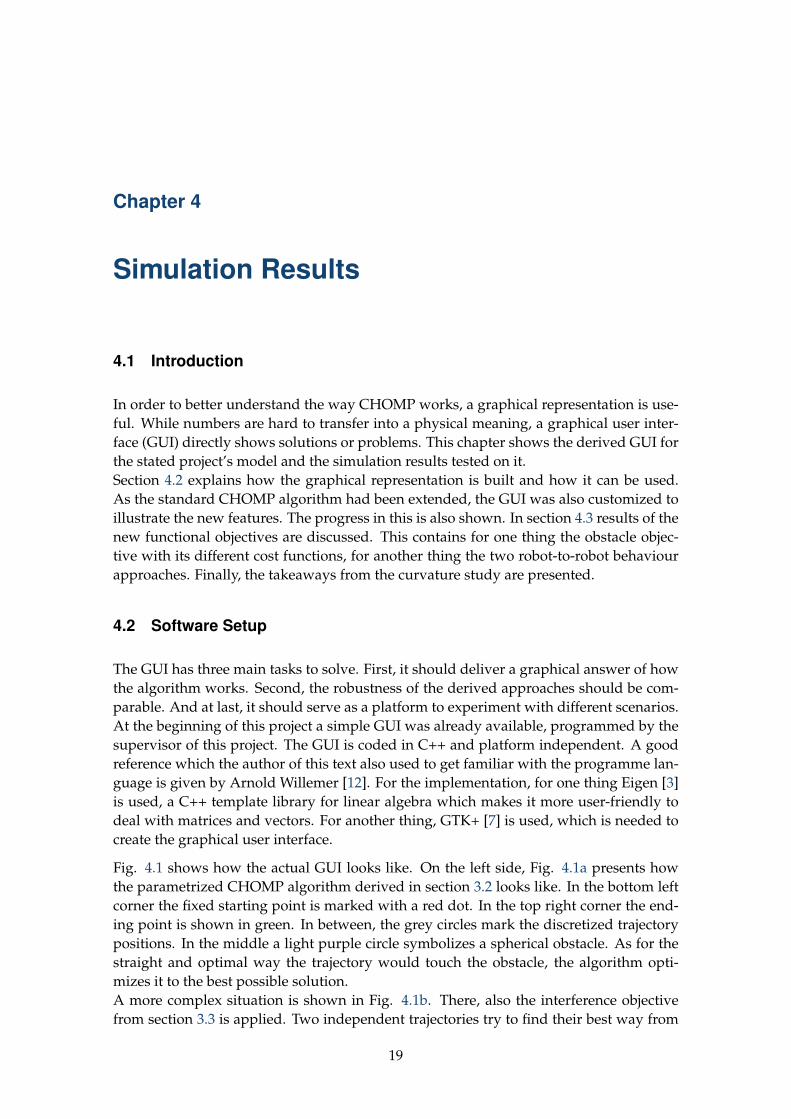
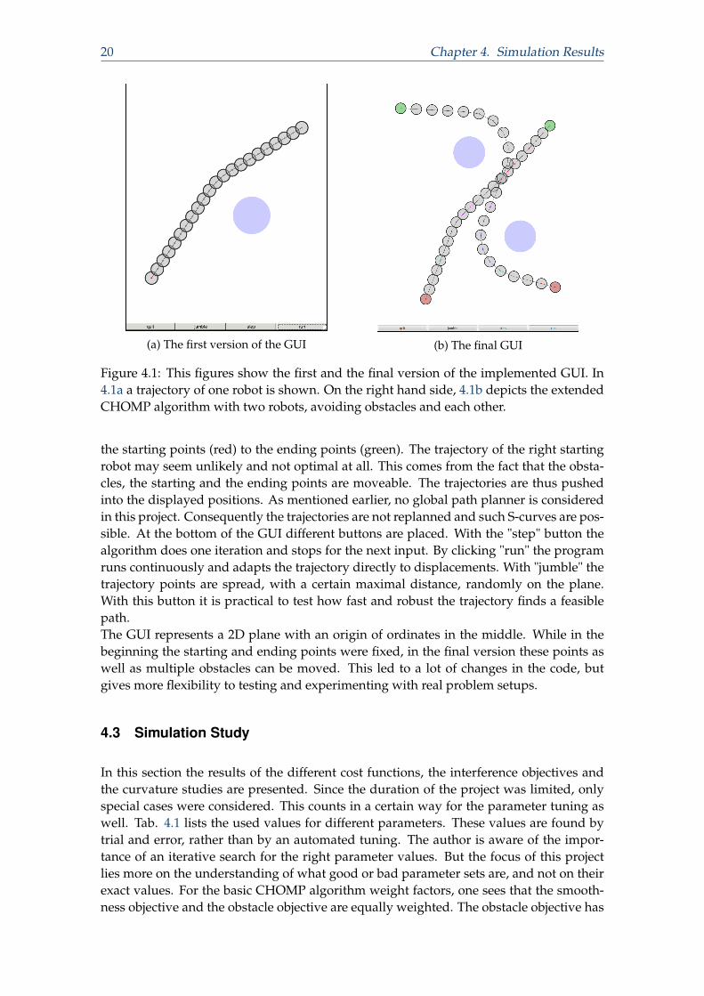
Fig. 4.1 shows how the actual GUI looks like. On the left side, Fig. 4.1a presents howthe parametrized CHOMP algorithm derived in section 3.2 looks like. In the bottom leftcorner the fixed starting point is marked with a red dot. In the top right corner the end-ing point is shown in green. In between, the grey circles mark the discretized trajectorypositions. In the middle a light purple circle symbolizes a spherical obstacle. As for thestraight and optimal way the trajectory would touch the obstacle, the algorithm opti-mizes it to the best possible solution.A more complex situation is shown in Fig. 4.1b. There, also the interference objectivefrom section 3.3 is applied. Two independent trajectories try to find their best way from

19

20 Chapter 4. Simulation Results

(a) The first version of the GUI (b) The final GUI

Figure 4.1: This figures show the first and the final version of the implemented GUI. In4.1a a trajectory of one robot is shown. On the right hand side, 4.1b depicts the extendedCHOMP algorithm with two robots, avoiding obstacles and each other.

the starting points (red) to the ending points (green). The trajectory of the right startingrobot may seem unlikely and not optimal at all. This comes from the fact that the obsta-cles, the starting and the ending points are moveable. The trajectories are thus pushedinto the displayed positions. As mentioned earlier, no global path planner is consideredin this project. Consequently the trajectories are not replanned and such S-curves are pos-sible. At the bottom of the GUI different buttons are placed. With the "step" button thealgorithm does one iteration and stops for the next input. By clicking "run" the programruns continuously and adapts the trajectory directly to displacements. With "jumble" thetrajectory points are spread, with a certain maximal distance, randomly on the plane.With this button it is practical to test how fast and robust the trajectory finds a feasiblepath.The GUI represents a 2D plane with an origin of ordinates in the middle. While in thebeginning the starting and ending points were fixed, in the final version these points aswell as multiple obstacles can be moved. This led to a lot of changes in the code, butgives more flexibility to testing and experimenting with real problem setups.

4.3 Simulation Study

In this section the results of the different cost functions, the interference objectives andthe curvature studies are presented. Since the duration of the project was limited, onlyspecial cases were considered. This counts in a certain way for the parameter tuning aswell. Tab. 4.1 lists the used values for different parameters. These values are found bytrial and error, rather than by an automated tuning. The author is aware of the impor-tance of an iterative search for the right parameter values. But the focus of this projectlies more on the understanding of what good or bad parameter sets are, and not on theirexact values. For the basic CHOMP algorithm weight factors, one sees that the smooth-ness objective and the obstacle objective are equally weighted. The obstacle objective has

4.3. Simulation Study 21

no parameter because it is taken as a reference, with a value equal to one. Interestingly,the interference objective weight factor µ has to be smaller than one, i.e. the other twoobjectives get more influence in terms of optimizing the trajectory. If µ is µ = 1 too, thetrajectories begin to oscillate if they are close to each other. For η and dt also other valuescan be taken without problem. The provided ones in Tab. 4.1 are a good trade-off in therequired time of finding a local minimum and the robustness of the computed trajectory.For example, if η = 10 a path is computed in only a couple of steps. But the points do notfind an equilibrium and they vibrate around the optimal path. In contrast, for η = 500the final trajectory is reached very slowly.

Symbol Description Value

λ Smoothness objective weight factor 1.0µ Interference objective weight factor 0.40η Regularization coefficient for gradient descent 100.0n Number of waypoints per trajectory 20dt Time step size 1.0

Table 4.1: Parameter values

4.3.1 Robot-to-Obstacle Performance

Considering the two functional objectives Fobs and Fsmooth, presented in [13], the focuslies on how the trajectory reacts to obstacles. For one robot CHOMP produces smoothtrajectories within a few numbers of iterations. The simulations with the programmedGUI are very satisfying. Hence the derivations made in section 3.2 are correct and usefulfor the project’s purpose. The applied discretization is intuitive but provides still flexibil-ity for changes or extensions.A decision every user can make is the choice of the cost function for Fobs. In section 3.2.2two possible obstacle cost functions are presented. Primarily both cost functions workimpeccably for the given representation. Differences appear if the trajectory’s propaga-tion gets close to obstacles. While cCHOMP already pushes the points away, ccubic doesn’treact at all. On the other hand, if the robot points are very close, ccubic suddenly pushesthem away even harder. Therefore, this cost function is more aggressive. This leads tomore oscillation of the trajectory, but on the other hand it may be helpful in a clutteredenvironment.Besides the two cost functions from above also other weighting policies are possible. Forexample in a higher dimensional case, a more problem-specific cost function could benecessary.

4.3.2 Robot-to-Robot Performance

In a multiple robot situation, every robot seeks for his own optimal trajectory. To handleupcoming collisions, an interference objective Fint was derived earlier in section 3.3.1.There, two different approaches are presented without advising which one suits the givenrepresentation better. At this point, it is firstly emphasized that both approaches areworking nicely and either of them has its advantages and drawbacks. Nevertheless, insome cases one is stretched to its limits. An impression therefore is given in Fig. 4.2.


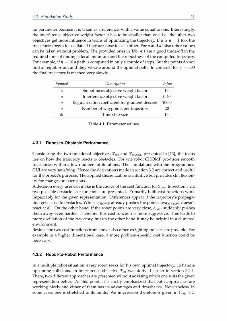
(a) Unit vector approach: both robots drivethe exact path with the same speed. Theywould collide on the vertical symmetry linebelow the obstacle.

(b) Obstacle function approach: the robotstarting on the left goes a little slowerand more downwards than the robot whichstarts from the right. They thus pass eachother slightly to the left of the symmetryline.

Figure 4.2: Both figures show an identical scenario, where an obstacle is placed on thesymmetrical line. While the obtained solution is not feasible with the unit vector ap-proach (4.2a), the trajectory is more sophisticated with the obstacle function approach(4.2b).

There, two robots have to circle an obstacle first and head to the ending points afterwards.While both approaches find a solution, the unit vector one in Fig. 4.2a is not possible.The robots would collide in the middle directly under the obstacle. The reason whythe algorithm fails is because the unit vectors are orthogonal to the obstacle functionalgradient vector. With the obstacle function approach shown in Fig. 4.2b this does nothappen since the gradient objective vectors stand with an angle to each other. This leadsto an offset which can be enlarged by a bigger robot-to-robot distance threshold.

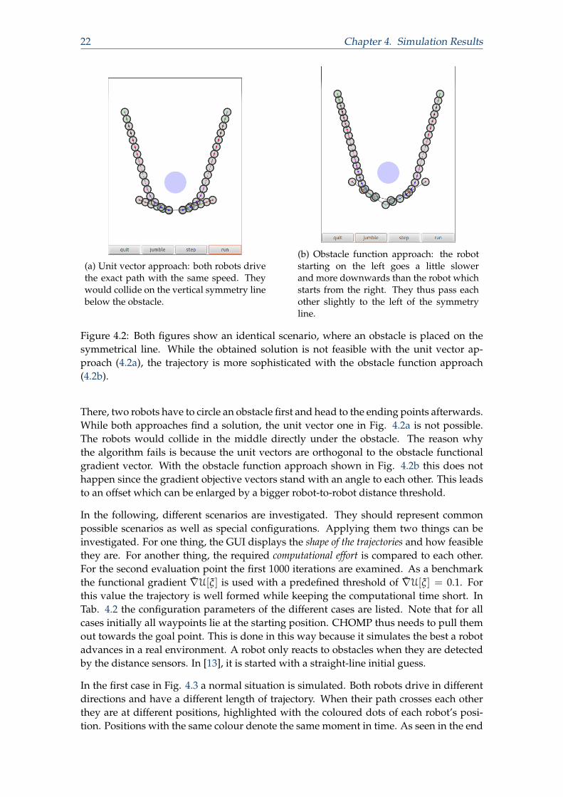
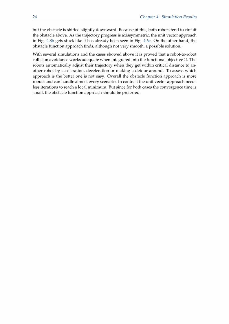
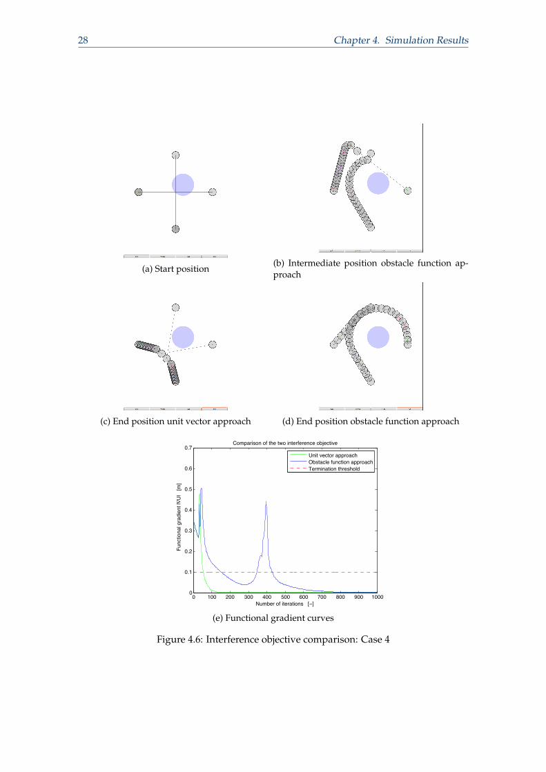
In the following, different scenarios are investigated. They should represent commonpossible scenarios as well as special configurations. Applying them two things can beinvestigated. For one thing, the GUI displays the shape of the trajectories and how feasiblethey are. For another thing, the required computational effort is compared to each other.For the second evaluation point the first 1000 iterations are examined. As a benchmarkthe functional gradient ∇̄U[ξ] is used with a predefined threshold of ∇̄U[ξ] = 0.1. Forthis value the trajectory is well formed while keeping the computational time short. InTab. 4.2 the configuration parameters of the different cases are listed. Note that for allcases initially all waypoints lie at the starting position. CHOMP thus needs to pull themout towards the goal point. This is done in this way because it simulates the best a robotadvances in a real environment. A robot only reacts to obstacles when they are detectedby the distance sensors. In [13], it is started with a straight-line initial guess.

In the first case in Fig. 4.3 a normal situation is simulated. Both robots drive in differentdirections and have a different length of trajectory. When their path crosses each otherthey are at different positions, highlighted with the coloured dots of each robot’s posi-tion. Positions with the same colour denote the same moment in time. As seen in the end


Case qs1 qe1 qs2 qe2 Obstacle

1 −4.0,−7.0 3.0, 8.0 3.0,−3.0 −5.0, 2.0 1.0, 1.02 −5.0,−5.0 7.0, 7.0 5.0,−5.0 −7.0, 7.0 1.0, 3.03 −5.0,−5.0 7.0, 7.0 −5.0,−8.0 7.0, 4.0 3.0,−1.04 0.0,−5.0 0.0, 5.0 −5.0, 0.0 5.0, 0.0 1.0, 1.05 5.0, 0.0 −5.0, 0.0 −5.0, 0.0 5.0, 0.0 0.0, 0.06 5.0, 0.0 −5.0, 0.0 −5.0, 0.0 5.0, 0.0 0.0,−0.50

Table 4.2: Configuration parameters for starting points qs1, qs2 of the first and secondrobot, ending points qe1, qe2 and the obstacle position. The units for the given x- andy-coordinates are in pixels and dynamically scaled to the size of the GUI window.

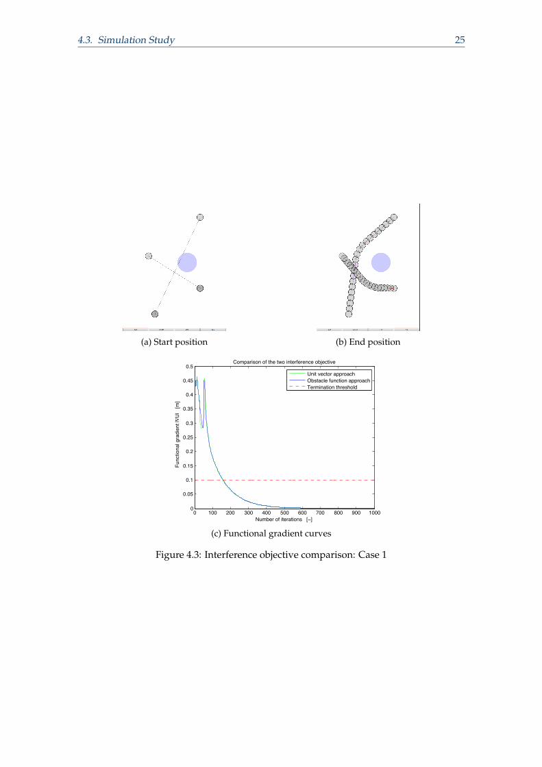
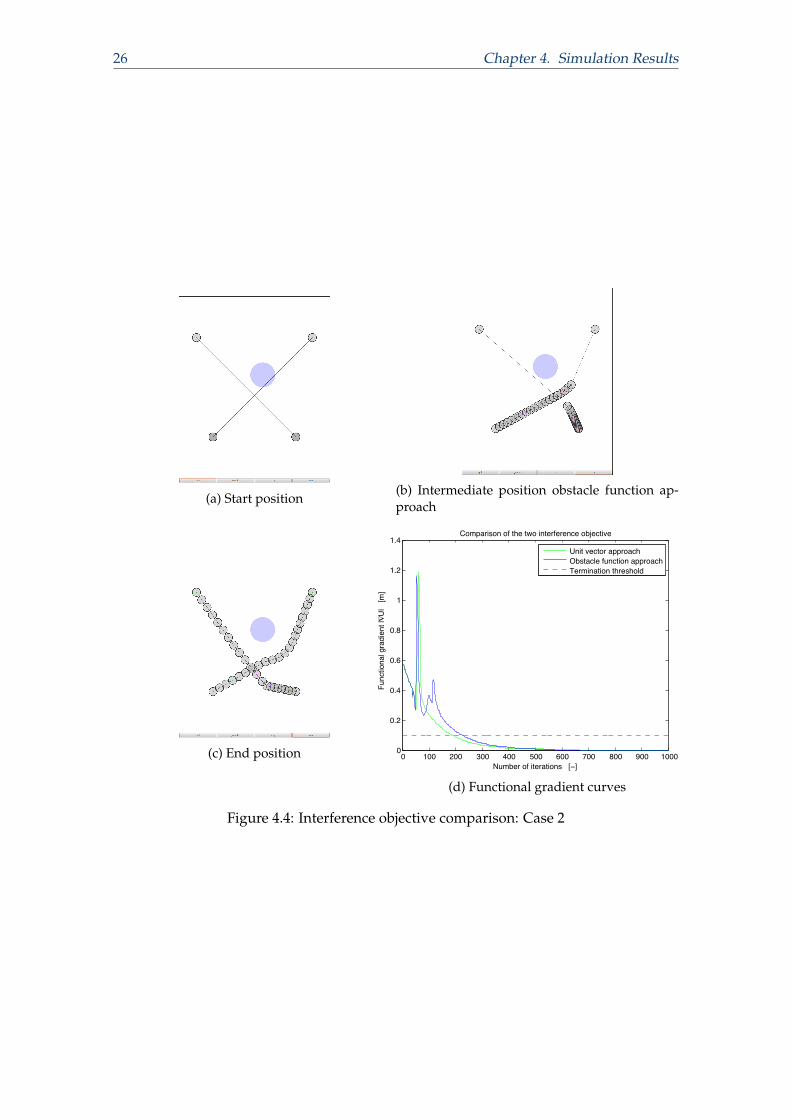
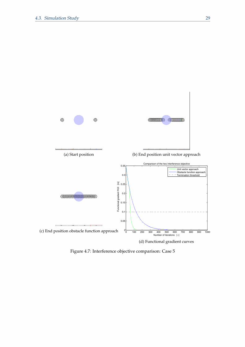
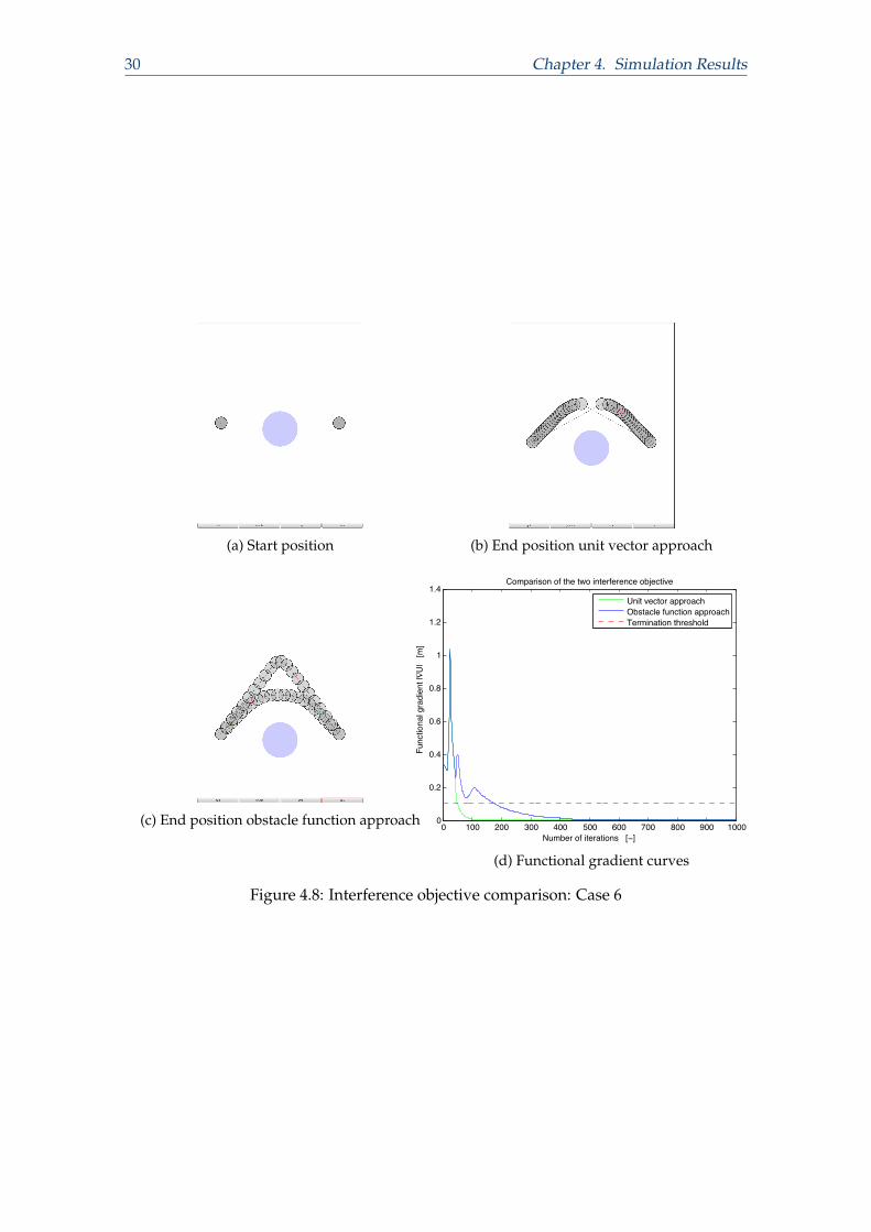
position Fig. 4.3b, the robots do not disturb each other. Thus the curves of the gradientdescent are identical.Case 2 (Fig. 4.4) shows symmetric starting and ending points and an obstacle shiftedslightly to the right. The right starting robot reaches the obstacle first and is pusheddownward. Because the left robot has to pass right after, the right robot is stronglypushed back, seen in Fig. 4.4b. This leads to strong corrections in the trajectory opti-mization and to the peak in Fig. 4.4d. In the end, for both approaches results the sametrajectory. Fig. 4.4c shows nicely how the right robot drives more slowly in the beginningto pass the other robot in accordance with the predefined minimal distance.Fig. 4.5 points out that the solutions for both approaches might be different. In this casethe inlying robot needs to avoid the obstacle first and because of the shift of his trajectory,the outer robot has to avoid the other one. Fig. 4.5b and 4.5c show nicely how this canbe done in two ways. In Fig. 4.5b the outer robot drives faster in the beginning to gopast before the other robot. As an advantage both robots drive their optimal path. On theother hand for the obstacle function approach (Fig. 4.5c) the total energy needed is lessbecause there is no acceleration or deceleration along the trajectory. In return the outerrobot drives a longer route. One remark to the obstacle functional gradient curve. Onenotices that the curve does not fall to zero after ∼ 400 iterations. The reason therefore isa continuous harmonic oscillation of near trajectory points in the first half.In case 4, Fig. 4.6a shows a situation which has a positive diagonal symmetry. Here it getsclear why the unit vector approach struggles with symmetric situations. While for thiscase the obstacle function approach finds a feasible solution (Fig. 4.6d), the unit vectorapproach gets caught by the other robot. The reason, therefore, is the same as explainedearlier. The update step falls in a bad equilibrium, where the smoothness, the obstacleand the interference objective gradient cancel each other out. The two peaks of the ob-stacle function approach in Fig. 4.6e are, on the one hand, for when the robots hit theobstacle and, on the other hand, when they have to avoid each other, seen in Fig. 4.6b. Inthis case the termination threshold is too high and should be set below ∇̄U[ξ] = 0.03.A special scenario shows case 5 (Fig. 4.7). There, each robot’s starting point lies on theothers ending point. The obstacle is located exactly in the middle. As both end positions(Fig. 4.7b and Fig. 4.7c) illustrate, both approaches cannot handle two starting lines witha straight angle between them and and an obstacle centred in the middle. Both robotsignore the obstacle in this case. While with the unit vector approach the trajectory stopswhen the robots get close to each other, the trajectories go straight through with the ob-stacle function approach.Finally case 6 is a small modification of case 5. The robot configurations are the same


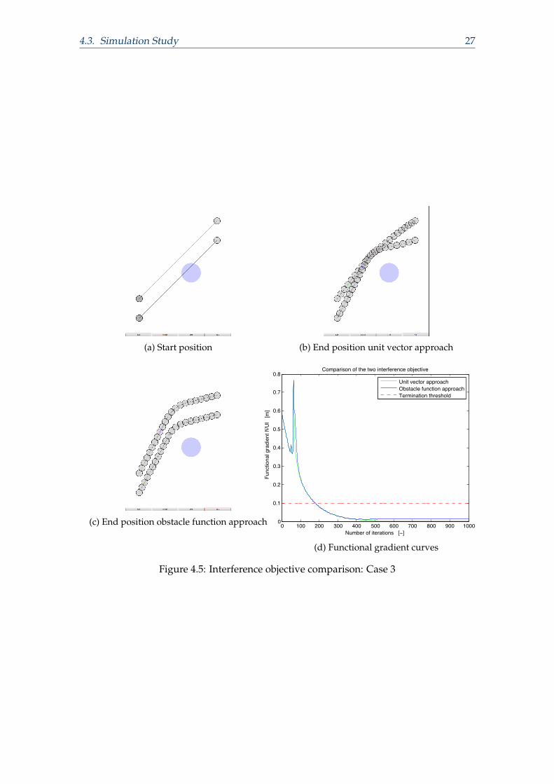
but the obstacle is shifted slightly downward. Because of this, both robots tend to circuitthe obstacle above. As the trajectory progress is axissymmetric, the unit vector approachin Fig. 4.8b gets stuck like it has already been seen in Fig. 4.6c. On the other hand, theobstacle function approach finds, although not very smooth, a possible solution.

With several simulations and the cases showed above it is proved that a robot-to-robotcollision avoidance works adequate when integrated into the functional objective U. Therobots automatically adjust their trajectory when they get within critical distance to an-other robot by acceleration, deceleration or making a detour around. To assess whichapproach is the better one is not easy. Overall the obstacle function approach is morerobust and can handle almost every scenario. In contrast the unit vector approach needsless iterations to reach a local minimum. But since for both cases the convergence time issmall, the obstacle function approach should be preferred.


(a) Start position (b) End position

0 100 200 300 400 500 600 700 800 900 10000

0.05

0.1

0.15

0.2

0.25

0.3

0.35

0.4

0.45

0.5Comparison of the two interference objective

Number of iterations [−]

Func

tiona

l gra

dien

t |∇U|

[m

]

Unit vector approachObstacle function approachTermination threshold

(c) Functional gradient curves

Figure 4.3: Interference objective comparison: Case 1


(a) Start position(b) Intermediate position obstacle function ap-proach

(c) End position 0 100 200 300 400 500 600 700 800 900 10000

0.2

0.4

0.6

0.8

1

1.2



Func

tiona

l gra

dien

t |∇U|

[m

]


(d) Functional gradient curves



(a) Start position (b) End position unit vector approach

(c) End position obstacle function approach 0 100 200 300 400 500 600 700 800 900 10000

0.1

0.2

0.3

0.4

0.5

0.6

0.7



Func

tiona

l gra

dien

t |∇U|

[m

]





(a) Start position(b) Intermediate position obstacle function ap-proach

(c) End position unit vector approach (d) End position obstacle function approach

0 100 200 300 400 500 600 700 800 900 10000

0.1

0.2

0.3

0.4

0.5

0.6



Func

tiona

l gra

dien

t |∇U|

[m

]


(e) Functional gradient curves





0.05

0.1

0.15

0.2

0.25

0.3



Func

tiona

l gra

dien

t |∇U|

[m

]







0.2

0.4

0.6

0.8

1

1.2



Func

tiona

l gra

dien

t |∇U|

[m

]





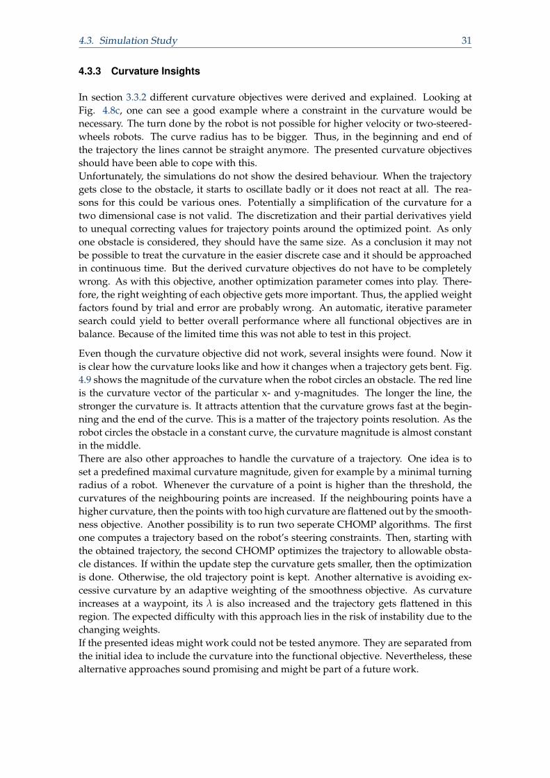
4.3.3 Curvature Insights

In section 3.3.2 different curvature objectives were derived and explained. Looking atFig. 4.8c, one can see a good example where a constraint in the curvature would benecessary. The turn done by the robot is not possible for higher velocity or two-steered-wheels robots. The curve radius has to be bigger. Thus, in the beginning and end ofthe trajectory the lines cannot be straight anymore. The presented curvature objectivesshould have been able to cope with this.Unfortunately, the simulations do not show the desired behaviour. When the trajectorygets close to the obstacle, it starts to oscillate badly or it does not react at all. The rea-sons for this could be various ones. Potentially a simplification of the curvature for atwo dimensional case is not valid. The discretization and their partial derivatives yieldto unequal correcting values for trajectory points around the optimized point. As onlyone obstacle is considered, they should have the same size. As a conclusion it may notbe possible to treat the curvature in the easier discrete case and it should be approachedin continuous time. But the derived curvature objectives do not have to be completelywrong. As with this objective, another optimization parameter comes into play. There-fore, the right weighting of each objective gets more important. Thus, the applied weightfactors found by trial and error are probably wrong. An automatic, iterative parametersearch could yield to better overall performance where all functional objectives are inbalance. Because of the limited time this was not able to test in this project.

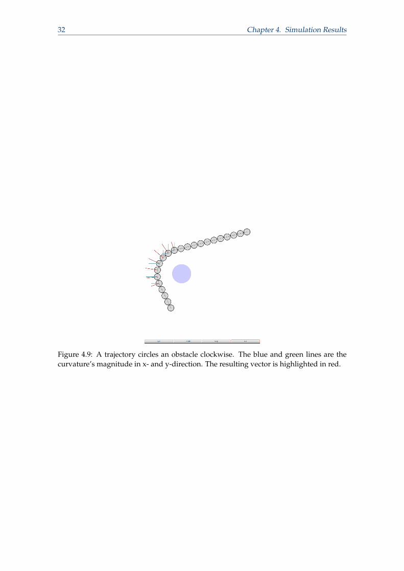
Even though the curvature objective did not work, several insights were found. Now itis clear how the curvature looks like and how it changes when a trajectory gets bent. Fig.4.9 shows the magnitude of the curvature when the robot circles an obstacle. The red lineis the curvature vector of the particular x- and y-magnitudes. The longer the line, thestronger the curvature is. It attracts attention that the curvature grows fast at the begin-ning and the end of the curve. This is a matter of the trajectory points resolution. As therobot circles the obstacle in a constant curve, the curvature magnitude is almost constantin the middle.There are also other approaches to handle the curvature of a trajectory. One idea is toset a predefined maximal curvature magnitude, given for example by a minimal turningradius of a robot. Whenever the curvature of a point is higher than the threshold, thecurvatures of the neighbouring points are increased. If the neighbouring points have ahigher curvature, then the points with too high curvature are flattened out by the smooth-ness objective. Another possibility is to run two seperate CHOMP algorithms. The firstone computes a trajectory based on the robot’s steering constraints. Then, starting withthe obtained trajectory, the second CHOMP optimizes the trajectory to allowable obsta-cle distances. If within the update step the curvature gets smaller, then the optimizationis done. Otherwise, the old trajectory point is kept. Another alternative is avoiding ex-cessive curvature by an adaptive weighting of the smoothness objective. As curvatureincreases at a waypoint, its λ is also increased and the trajectory gets flattened in thisregion. The expected difficulty with this approach lies in the risk of instability due to thechanging weights.If the presented ideas might work could not be tested anymore. They are separated fromthe initial idea to include the curvature into the functional objective. Nevertheless, thesealternative approaches sound promising and might be part of a future work.


Figure 4.9: A trajectory circles an obstacle clockwise. The blue and green lines are thecurvature’s magnitude in x- and y-direction. The resulting vector is highlighted in red.

Chapter 5

Conclusion and Future Work

5.1 Introduction

In this chapter, a conclusion of the presented results from chapter 4 is given. The goalsof the project are reflected again and compared with the obtained results. Additionally,an outlook on possible future work in the field of motion planning and the CHOMPalgorithm in particular is provided.

5.2 Evaluation of the Project

Based on the stated goals in section 1.1 and the simulation results in section 4.3 the workis summarized below.

• In a first step the CHOMP algorithm was successfully adapted to the stated repre-sentation. Therefore, the presented theory in [13] had to be investigated and under-stood. The functional objectives are now given in an adapted form for a 2D planerepresentation. For this, discrete gradient functional objectives and necessary ma-trices and vectors are derived.

• Out of the adapted trajectory optimization technique a graphical representationwas implemented. It represents simple robot motions in a flat terrain. With thisGUI the investigated optimization technique is understood much better. While itis easy to use, simulations and testing can be done with it. Therefore, it serves asa handy platform to investigate new ideas or combinations with other techniques.The results show that CHOMP is highly valuable for use in the underlying projectof this work. This algorithm performs in a fast way and with less computationalcosts than other techniques. It provides smooth and collision free paths while seek-ing for an optimal trajectory.

• An important goal of this thesis was the extension to a multiple robot representa-tion. Therefore the required matrices and vectors were adapted and a new func-tional objective was built directly into the CHOMP algorithm. Two different ap-proaches were derived and tested against each other. While the unit vector ap-proach needs less computational cost to converge to a local minimum, the obstaclefunction approach handles more tricky situations better. As a consequence, the ob-stacle function approach is to prefer if the number of robots is small. For higher

33

34 Chapter 5. Conclusion and Future Work

number of robots this may not be the case anymore. In general the presented tech-nique to deal with robot-to-robot avoidance works very well and is robust as manysimulations have shown. The use of this extended algorithm for future projects canbe highly recommended.

• Various attempts tried to integrate curvature constraints of nonholonomic robots.Even if this did not work, the graphical representations and various simulations ledto a deeper understanding of it. As a result, possible alternatives are presented. Afinal refusal to integrate the curvature into the objective functional should not bedone as long as other approaches still are possible.

In summary, the existing path adaption technique is successfully extended for multiplerobots. A graphical representation is implemented and used for simulation and testing.This GUI can be used for further developments and validations. With the acquired feelingfor curvature behaviour, possibilities and limits are more clear and other approaches aredevised.

5.3 Future Work

During the time of this project, new and interesting questions arose which could not beanswered up to this moment. Possible future work in the field of trajectory optimizationare the following.

• It is desirable to obtain a method which successfully treats curvature constraintsof wheeled robots. The possible approaches presented in section 4.3.3 are ready forimplementation and testing. A new derivation of the functional gradient by solvingthe Lagrangian form of an optimization problem may lead to the desired behaviour.

• So far, for every trajectory the number of trajectory points are the same. As a con-sequence, the robots reach their ending point at the same time. While a robot witha long path drives fast, a robot with a short route has to drive slowly. With a dis-engagement of this constraint the robots could move closer to their velocity andacceleration limits. The goal points are reached faster and the possibility of a col-lision is smaller. Whether one should implement the variable number of trajectorypoints inside CHOMP or deal this as an outer motion planner has to be determined.

• For the simulation always two robots were considered. With this it has been proventhat the algorithm also works for multiple robots. To simulate a variable numberof robots, the established code has to be changed in order to automatically adjustmatrix and vector sizes. The derivations presented in chapter 3 remain the sameand can be directly modified in the explained way.

Appendix

A Partial Derivatives for the 2D Curvature Representation

In section 3.3.2 two different approaches for a possible curvature objective are presented.For the first one, Eq. (3.22) expresses the discrete gradient objective. Within this equationthe gradient∇κt is needed. This appendix presents the partial derivatives which are usedfor the implementation. They have been computed with Mathematica®, a computationalsoftware program.In the discrete case, the velocity and the acceleration are computed via finite differences.For the velocity, one can choose between forward, average or backward velocity. Startingfrom the actual trajectory point qi, the forward velocity would be q

′i =

qi+1−qi∆t , where qi+1

is the trajectory point after qi. This leads to a drift of the trajectory points into the directionof the goal point because only the path in front of qi is regarded and not what is behind qi.Therefore the average velocity and the average acceleration is used for implementation:

q′i =

qi+1 − qi−1

2∆t, (A.1)

q′′i =

q′+i − q

′−i

∆t=

qi+1 − 2qi + qi−1

∆t2 . (A.2)

In Eq. (A.2), q′+i stands for the forward velocity and q

′−i for the backward velocity. This

representation of the velocity and acceleration is used in Eq. (3.20) to form the discretecurvature. First, in Fig. A.1 one can see how the curvature looks like when the expressionis expanded. Out of this, the partial derivatives are computed and presented in Fig. A.2.

35

36 Appendix

��

� = ��((�� - ��) / (� * ��)) * �� - � * �� + �� -

�((�� - ��) / (� * ��)) * �� - � * �� + �� ((�� - ��) / (� * ��))�� + �((�� - ��) / (� * ��))��(� / �)�

- (-� ��+��+��) (-��+��)� �� + (-��+��) (-� ��+��+��)

� ��

� (-��+��)�� + (-��+��)�

� �� /�

��[�]

� �� -�� + �� + �� - �� + �� (-�� + ��)�

�� -� �� +��+(��-��)��

�/�

�� = ��[�� > �]

� �� -�� + �� + �� - �� + �� (-�� + ��)�

�� - � �� + �� + (�� - ��)��/�

��[�]

��

�� (-��+��)�� + (-��+��)�

� �� /�

-��

�� (-��+��)�� + (-��+��)�

� �� /�

-

��

�� (-��+��)�� + (-��+��)�

� �� /�

+��

�� (-��+��)�� + (-��+��)�

� �� /�

+

��

�� (-��+��)�� + (-��+��)�

� �� /�

-��

�� (-��+��)�� + (-��+��)�

� �� /�

��

�[�� ]

� �� - ��

�� - � �� + �� + (�� - ��)��/�-

�� (� �� - � ��) �� -�� + �� + �� - �� + �� (-�� + ��)�

�� - � �� + �� + (�� - ��)��/�

�[�� ]

� (-�� + ��)

�� - � �� + �� + (�� - ��)��/�

�[�� ]

� �-�� + ��

�� - � �� + �� + (�� - ��)��/�-

�� (-� �� + � ��) �� -�� + �� + �� - �� + �� (-�� + ��)��

�� - � �� + �� + (�� - ��)��/�

��

Figure A.1: The 2D curvature representation of Eq. (3.20) is expanded in a first step. "xp1"stands for the first entry in qi+1 and "yp1" the second entry respectively. "xi" and "yi" arethe entries in qi and "xm1" and "ym1" are the entries in qi−1.

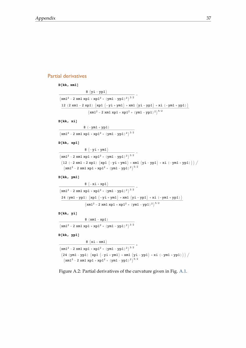
Appendix 37

��

�[�� ]

� �� - ��

�� - � �� + �� + (�� - ��)��/�-

�� (� �� - � ��) �� -�� + �� + �� - �� + �� (-�� + ��)�

�� - � �� + �� + (�� - ��)��/�

�[�� ]

� (-�� + ��)

�� - � �� + �� + (�� - ��)��/�

�[�� ]

� �-�� + ��

�� - � �� + �� + (�� - ��)��/�-

�� (-� �� + � ��) �� -�� + �� + �� - �� + �� (-�� + ��)��

�� - � �� + �� + (�� - ��)��/�

�[�� ]

� �-�� + ��

�� - � �� + �� + (�� - ��)��/�-

�� (�� - ��) �� -�� + �� + �� - �� + �� (-�� + ��)�

�� - � �� + �� + (�� - ��)��/�

�[�� ]

� (�� - ��)

�� - � �� + �� + (�� - ��)��/�

�[�� ]

� �� - ��

�� - � �� + �� + (�� - ��)��/�+

�� (�� - ��) �� -�� + �� + �� - �� + �� (-�� + ��)��

�� - � �� + �� + (�� - ��)��/�

��

Figure A.2: Partial derivatives of the curvature given in Fig. A.1.

38 Appendix

Bibliography

[1] Cargo-ANTs. Poster Cargo-ANTs, 2013 (accessed December 01, 2014). http://cargo-ants.eu/index.php/downloads.

[2] Community Research and Development Information Service (CORDIS). Cargo-Ants, 2013 (accessed November 28, 2014). http://cordis.europa.eu/project/rcn/110967_en.html.

[3] Gaël Guennebaud and Benoît Jacob and others. Eigen v3, 2010 (accessed January 09,2015). http://eigen.tuxfamily.org.

[4] S. Karaman and E. Frazzoli. Sampling-based algorithms for optimal motion plan-ning. International Journal of Robotics Research, 30(7):846–894, June 2011.

[5] Steven M. LaValle. Planning Algorithms. Cambridge University Press, 2006.

[6] Steven M. LaValle, Michael S. Branicky, and Stephen R. Lindemann. On the Relation-ship between Classical Grid Search and Probabilistic Roadmaps. The InternationalJournal of Robotics Research, 23(7-8):673–692, 2004.

[7] Matthias Clasen and others. The GTK+ Project, 2007 (accessed January 09, 2015).http://www.gtk.org.

[8] Roland Philippsen and Roland Yves Siegwart. Smooth and efficient obstacle avoid-ance for a tour guide robot. In ICRA, pages 446–451, 2003.

[9] Sean Quinlan. Real-time modification of collision-free paths. PhD thesis, Stanford Uni-versity, 12 1994.

[10] Roland Siegwart, Illah Reza Nourbakhsh, and Davide Scaramuzza. Introduction toautonomous mobile robots. MIT Press, 2011.

[11] Wikipedia. Curvature — Wikipedia, the free encyclopedia, 2015 (accessed January08, 2015). http://en.wikipedia.org/wiki/Curvature.

[12] Arnold Willemer. Einstieg in C++. Galileo Press, 2009.

[13] Matt Zucker, Nathan Ratliff, Anca D. Dragan, Mihail Pivtoraiko, Matthew Klin-gensmith, Christopher M. Dellin, J. Andrew Bagnell, and Siddhartha S. Srinivasa.CHOMP: Covariant Hamiltonian optimization for motion planning. The Interna-tional Journal of Robotics Research, 32(9-10):1164–1193, 2013.

39

http://cargo-ants.eu/index.php/downloads

http://cargo-ants.eu/index.php/downloads

http://cordis.europa.eu/project/rcn/110967_en.html

http://cordis.europa.eu/project/rcn/110967_en.html

http://eigen.tuxfamily.org

http://www.gtk.org

http://en.wikipedia.org/wiki/Curvature

Documents

Investigation of Trajectory Optimization for Multiple …hh.diva-portal.org/smash/get/diva2:1072005/FULLTEXT01.pdf · Investigation of Trajectory Optimization for Multiple Car-Like