Ionospheric Correction Algorithm for Galileo Single ... · iii ionospheric correction algorithm for galileo single freuenc users, issue 1.2, september 2016 table of contents section

IonospherIc correctIon AlgorIthm for gAlIleo sIngle frequency users

EuropEan GnSS (GalilEo) opEn SErvicENAVIGATION

SOLUTIONS

POWERED BY

E U R O P E

Document subject to terms of use AnD DIsclAImers pAge.i

© european commission, 2016

European GNSS (Galileo) Open Service – Ionospheric Correction

Algorithm for Galileo Single Frequency Users

i

I o n o s p h e r I c c o r r e c t I o n A l g o r I t h m f o r g A l I l e o s I n g l e f r e q u e n c y u s e r s , I s s u e 1 . 2 , s e p t e m b e r 2 0 1 6

TERMS OF USE AND DISCLAIMERS

this document describes the ionospheric model developed for the galileo satellite navigation system, which can be used to determine galileo single-frequency ionospheric corrections. Its content has been prepared and scrutinised by various groups of specialised scientists. the model has been characterised and thoroughly tested and gives encouraging performance improvements compared to other currently used solutions. the physical behaviour of the ionosphere is however such that one cannot produce an algorithm that will systematically deliver fully satisfactory compensation of ionospheric error under all conditions.

the european commission, esA, the author(s) or contributor(s) therefore do not assume any responsibility whatsoever for its use, and do not make any guarantee, expressed or implied, about the quality, reliability, suitability for any particular use or any other characteristic of the algorithm. under no circumstances shall the european commission, european union, esA, the author(s) or contributor(s) be liable for damages resulting directly or indirectly from the use, misuse or inability to use the algorithm.

ACkNOwLEDgEMENTS

the NeQuick electron density model was developed by the Abdus salam International center of theoretical physics (Ictp) and the university of graz. the adaptation of NeQuick for the galileo single-frequency ionospheric correction algorithm (NeQuick g) has been performed by the european space Agency (esA) involving the original authors and other european ionospheric scientists under various esA contracts. the step-by-step algorithmic description of NeQuick for galileo contained in this document has been a collaborative effort of icTp, ESa and the european commission, including jrc.

ii

DOCUMENT ChANgE RECORD

REASON FOR ChANGE ISSUE REvISION DAtE

first Issue 1 0 november 2014

Document ready for publication after revision 1 1 june 2015

Inclusion of errata 1 2 september 2016

iii


TAbLE OF CONTENTS

SECTION 1: INTrOduCTION ...............................................................................................................1

1.1 dOCumENT SCOpE ......................................................................................1

1.2 BaCkgrOuNd..................................................................................................1

SECTION 2: SINglE FrEquENCy IONOSphErIC COrrECTION algOrIThm.........................................................................................................................4

2.1 OvErvIEw ..........................................................................................................5

2.2 Step-by-Stepprocedure .................................................................5

2.3 INpuTS aNd OuTpuTS ...........................................................................6

2.3.1 galIlEO NavIgaTION mESSagE rElEvaNT TO Single-frequencyionoSphericalgorithm ......................6

2.4 mOdIp rEgIONS .............................................................................................6

2.5 NeQuick G IONOSphErIC ElECTrON dENSITy mOdE ......................................................................................................................7

2.5.1 ThE EpSTEIN FuNCTION .................................................................................7

2.5.2 CONSTaNTS uSEd ...............................................................................................8

2.5.3 COmplEmENTary FIlES .................................................................................8

2.5.3.1. MODIP grID ................................................................................................................8

2.5.3.2. CCIr fIles ...................................................................................................................8

2.5.4 auxIlIary paramETErS................................................................................8

2.5.4.1. lOCal TIMe ................................................................................................................9

2.5.4.2. reaD MODIPNeQg_wraPPeD.asC values IN aN array.......................................................................................................................9

2.5.4.3. COMPuTe MODIP .................................................................................................9

2.5.4.4. effeCTIve IONIsaTION level az .................................................10

2.5.4.5. EffEctivESunSpotnumbEr(r12likE) ............................10

2.5.4.6. sOlar DeClINaTION ....................................................................................10

2.5.4.7. sOlar zeNITh aNgle .................................................................................10

2.5.4.8. effeCTIve sOlar zeNITh aNgle .................................................11

2.5.5 mOdEl paramETErS .....................................................................................11

2.5.5.1. foe aND Nme ..........................................................................................................11

2.5.5.2. fof1 aND Nmf1 ....................................................................................................12

2.5.5.3. fof2 aND Nmf2;m(3000)f2 ...............................................................12

2.5.5.4. hMe ....................................................................................................................................15

2.5.5.5. hMf1 ................................................................................................................................15

2.5.5.6. hMf2 ................................................................................................................................16

2.5.5.7. B2BOT, B1TOP, B1BOT, BeTOP, BeBOT ......................................16

2.5.5.8. a1 .........................................................................................................................................16

2.5.5.9. a2 aND a3 ...............................................................................................................17

2.5.5.10. shaPe ParaMeTer k ......................................................................................................17

2.5.5.11. h0 .........................................................................................................................................18

2.5.6 ElECTrON dENSITy COmpuTaTION ..................................................18

2.5.6.1. The BOTTOMsIDe eleCTrON DeNsITy ..................................18

2.5.6.2. The TOPsIDe eleCTrON DeNsITy ...............................................19

2.5.7 auxIlIary rOuTINES ....................................................................................20

2.5.7.1. ThIrD OrDer INTerPOlaTION fuNCTION zx(Z1, z2, z3, z4,x) .............................................................................................20

2.5.8 TEC CalCulaTION ............................................................................................21

2.5.8.1. verTICal TeC CalCulaTION ..............................................................21

2.5.8.2. slaNT TeC CalCulaTION ......................................................................22

2.5.8.3. alTerNaTIve COMPuTaTIONal effICIeNT TeC INTegraTION MeThOD ..............................................................................28

2.5.9 ClarIFICaTION ON COOrdINaTES uSEd IN NeQuick ...............28

2.6 dIFFErENCES BETwEEN Nequick g aNd Nequick 1 aNd Nequick 2 ...................................................................28

2.6.1 Summary OF dIFFErENCES wITh NeQuick 1 .............................29

2.6.2 Summary OF dIFFErENCES wITh NeQuick 2 ............................29

SECTION 3: ImplEmENTaTION guIdElINES FOr uSEr rECEIvErS ............... 30

3.1 Zero-valuedcoefficientSanddefault EFFECTIvE IONISaTION lEvEl ........................................................31

3.2 applICaBIlITy aNd COhErENCE OF BrOadCaST COEFFICIENTS ..............................................................31

3.3 EFFECTIvE IONISaTION lEvEl BOuNdarIES .....................31

3.4 INTEgraTION OF NEquICk g INTO hIghEr lEvEl SOFTwarE .....................................................................................32

3.5 COmpuTaTION raTE OF IONOSphErIC COrrECTIONS ..............................................................................................32

iv

aNNEx a: applICaBlE aNd rEFErENCE dOCumENTS ....................................... 34

a.1. applICaBlE dOCumENTS .................................................................35

a.2. rEFErENCE dOCumENTS ...................................................................35

aNNEx B: aCrONymS aNd dEFINITIONS .........................................................................36

B.1. aCrONymS ......................................................................................................37

B.2. dEFINITIONS ..................................................................................................37

aNNEx C: complementaryfileS(ccirandmodip) ........................................ 40

aNNEx d: NEquICk g pErFOrmaNCE rESulTS .........................................................42

aNNEx E: INpuT/OuTpuT vErIFICaTION daTa ...........................................................48

E.1. azcoefficientS(highSolaractivity) ............................49

E.2. azcoefficientS(mediumSolaractivity) ...................50

E.3. azcoefficientS(lowSolaractivity) ............................51

aNNEx F: Nequick g dETaIlEd prOCESSINg mOdEl ............................................52

F.1. ExTErNal INTErFaCES ........................................................................53

F.1.1 INTrOduCTION ...................................................................................................53

f.1.1.1. INPuTs ...........................................................................................................................53

f.1.1.2. OuTPuTs .....................................................................................................................53

f.1.1.3. INPuT/OuTPuT ...................................................................................................53

F.2. mOdulES ........................................................................................................ 54

F.2.1 INTrOduCTION ...................................................................................................54

F.2.2 FuNCTION OvErvIEw ...................................................................................54

F.2.3 Nequick.c mOdulE ...........................................................................................55

f.2.3.1. fuNCTION ”NeQuick”(mainfunction)................................55

f.2.3.2. NeQuick INTerNal fuNCTION “NeQCheCkINPuTs” ......................................................................................56

f.2.3.3. NeQuick INTerNal fuNCTION “DOTeCINTegraTION” .................................................................................56

F.2.4 NEqCalCmOdIpaz.c mOdulE ................................................................58

f.2.4.1. NeQuick INTerNal fuNCTION “NeQCalCMODIP” ............................................................................................58

f.2.4.2. NeQuick INTerNal fuNCTION “NeQINTerPOlaTe” ........................................................................................59

f.2.4.3. NeQuick INTerNal fuNCTION “NeQMODIPTOaz” .............................................................................................60

F.2.5 NEqgETrayprOpErTIES.c mOdulE .................................................61

f.2.5.1. NeQuick INTerNal fuNCTION “NeQgeTrayPrOPerTIes” .....................................................................61

f.2.5.2. NeQuick INTerNal fuNCTION “NeQCalCrayPrOPerTIes1”...............................................................62

f.2.5.3. NeQuick INTerNal fuNCTION “NeQCalCrayPrOPerTIes2" ..............................................................63

F.2.6 NEqINTEgraTE.c mOdulE ........................................................................64

f.2.6.1. NeQuick INTerNal fuNCTION “NeQINTegraTe” .......64

F.2.7 NEqgETNEONvErTray.c mOdulE .....................................................66

f.2.7.1. NeQuick INTerNal fuNCTION “NeQgeTNeONverTICalray” ............................................................66

F.2.8 NEqgETNEONSlaNTray.c mOdulE .................................................67

f.2.8.1. NeQuick INTerNal fuNCTION “NeQgeTNeONslaNTray” ....................................................................67

f.2.8.2. NeQuick INTerNal fuNCTION “NeQCalCllhONray” ................................................................................ 68

F.2.9 NEqCalCEpSTparamS.c mOdulE .....................................................69

f.2.9.1. NeQuick INTerNal fuNCTION “NeQCalCePsTParaMs” ..........................................................................69

f.2.9.2. NeQuick INTerNal fuNCTION “NeQCalCsPhlegCOeffs” ...................................................................72

f.2.9.3. NeQuick INTerNal fuNCTION “NeQgeTf2freQfrOMCCIr” ...............................................................73

f.2.9.4. NeQuick INTerNal fuNCTION “NeQCrITICalfreQTONe” ......................................................................74

f.2.9.5. NeQuick INTerNal fuNCTION “NeQCalCf2PeakheIghT” ....................................................................75

f.2.9.6. NeQuick INTerNal fuNCTION “NeQePsTeIN”................76

F.2.10 NEqCalCTOpSIdE.c mOdulE .................................................................76

f.2.10.1. NeQuick INTerNal fuNCTION “NeQCalCTOPsIDeNe” ...............................................................................76

F.2.11 NEqCalCBOTTOmSIdENE.c mOdulE ..............................................77

f.2.11.1. NeQuick INTerNal fuNCTION “NeQCalCBOTTOMsIDeNe” ..................................................................77

F.2.12 NEquTIlS.c mOdulE .....................................................................................79

f.2.12.1. NeQuick INTerNal fuNCTION “NeQJOIN” ..........................79

f.2.12.2. NeQuick INTerNal fuNCTION “NeQClIPexP” ................79

f.2.12.3. NeQuick INTerNal fuNCTION “NeQsQuareD” ........... 80

F.3. Nequick FuNCTION daTa STruCTurES ................................. 80

v


LIST OF FIgURES

FiGurE 1. ExamplE oF a Global vTEc map obtAIneD wIth NeQuick ............................................3

fIgure 2. MODiP regIons AssocIAteD to DIfferent IonospherIc chArActerIstIcs ...............................................................7

fIgure 3. geometry of zenIth Angle computAtIon .....................................................................23

fIgure 4. geometry of rAy perIgee computAtIon .....................................................................24

FiGurE 5. ionoSphEric DElay vS. SaTElliTE ElEvaTion (uppEr) anD oF uTc (lowEr) .....................................................................................43

fIgure 6. performAnce of the gAlIleo sIngle frequency IonospherIc correctIon ......................................................................... 44

fIgure 7. globAl DAIly rms IonospherIc rESiDual Error [ml1] aFTEr correctIon wIth gAlIleo NeQuick g AnD gps IcA from AprIl 2013 to mArch 2014. .........................................................................45

FiGurE 8. rmS corrEcTion capabiliTy (%, wiTh a lowEr bounD oF 20 TEcu) of gAlIleo NeQuick g AnD gps IcA correctIon moDels for DAy 127, 2013 AnD DAy 80, 2014 ............................................46

FiGurE 9. rESiDual SinGlE-FrEquEncy rmS error contrIbutIon to uere After corrEcTion wiTh SinGlE-FrEquEncy ionoSphEric alGoriThm [ml1] ..........................47

FiGurE 10. ovErviEw oF NeQuick functIon hIerArchy ..............................................................................54

LIST OF TAbLES

tAble 1. Input pArAmeters ..........................................................6

tAble 2. DefInItIon of constAnts .......................................8

tAble 3. NeQuick functIon Input DAtA ........................53

tAble 4. NeQuick functIon output DAtA ...................53


tAble 6. neqcheckInputs functIon Input DAtA ..............................................................................................56

tAble 7. DotecIntegrAtIon functIon Input DAtA ..............................................................................................57


tAble 9. neqcAlcmoDIp functIon Input DAtA ..............................................................................................58

tAble 10. neqInterpolAte functIon Input DAtA ..............................................................................................59

tAble 11. neqcAlcmoDIp functIon Input DAtA ..............................................................................................60

tAble 12. neqgetrAypropertIes functIon Input/output DAtA ......................................................61

tAble 13. neqgetrAypropertIes functIon output DAtA .......................................................................61

tAble 14. neqcAlcrAypropertIes1 functIon Input/output DAtA ......................................................62

tAble 15. neqcAlcrAypropertIes1 functIon output DAtA .......................................................................62

tAble 16. neqcAlcrAypropertIes2 functIon Input DAtA .............................................................................63

tAble 17. neqcAlcrAypropertIes2 functIon Input/output DAtA ......................................................63

tAble 18. neqcAlcrAypropertIes2 functIon output DAtA .......................................................................63

tAble 19. neqIntegrAte functIon Input DAtA ..............................................................................................64

tAble 20. neqIntegrAte functIon output DAtA ..............................................................................................64

tAble 21. neqIntegrAte functIon Input/ output DAtA .......................................................................65

TablE 22. nEqGETnEonvErTray FuncTion Input DAtA .............................................................................66

TablE 23. nEqGETnEonvErTray FuncTion Input/output DAtA ......................................................67

tAble 24. neqgetneonslAntrAy functIon Input DAtA .............................................................................67

tAble 25. neqgetneonslAntrAy functIon output DAtA .......................................................................67

vi

tAble 26. neqgetneonslAntrAy functIon Input/output DAtA ......................................................67

tAble 27. neqcAlcllhonrAy functIon Input DAtA ..............................................................................................68

tAble 28. neqcAlcllhonrAy functIon output DAtA .......................................................................68

tAble 29. neqcAlcepstpArAms functIon Input DAtA .............................................................................69

tAble 30. neqcAlcepstpArAms functIon output DAtA .......................................................................69

tAble 31. neqcAlcepstpArAms functIon Input/output DAtA ......................................................70

tAble 32. neqcAlcsphlegcoeffs functIon Input DAtA .............................................................................73

tAble 33. neqcAlcsphlegcoeffs functIon Input/output DAtA ......................................................73

tAble 34. neqgetf2freqfromccIr functIon Input DAtA .............................................................................73

tAble 35. neqcrItIcAlfreqtone functIon Input DAtA .............................................................................74

tAble 36. neqcAlcf2peAkheIght functIon Input DAtA .............................................................................75

tAble 37. neqcAlcf2peAkheIght functIon Input DAtA .............................................................................75

tAble 38. neqcAlctopsIDene functIon Input DAtA ..............................................................................................76

tAble 39. neqcAlctopsIDene functIon output DAtA .......................................................................76

tAble 40. neqcAlcbottomsIDe functIon Input DAtA .............................................................................77

tAble 41. neqjoIn functIon Input DAtA ........................79

tAble 42. neqclIpexp functIon Input DAtA ...............80

tAble 43. neqsquAreD functIon Input DAtA ...........80

tAble 44. DefInItIon of NeQuickInputDAtA_st DAtA structure ..............................................................80

tAble 45. DefInItIon of MODiP_st DAtA structure ............................................................................81

tAble 46. DefInItIon of ccIr_st DAtA structure ............................................................................81

tAble 47. DefInItIon of spoInt_st DAtA structure ............................................................................81

tAble 48. DefInItIon of currentccIr_st DAtA structure ............................................................................81

tAble 49. DefInItIon of lAyerpropertIes_st DAtA structure ..............................................................82

tAble 50. DefInItIon of geometry_st DAtA structure ............................................................................82

tAble 51. DefInItIon of IntegrAteDAtA_st DAtA structure ..............................................................82

vii


SECTION 1: INTrOduCTION

1


1.1 DOCUMENT SCOpEthis document complements the galileo os sIs IcD [Annex A[1]] by describing in detail the reference algorithm to be implemented at user receivers to compute ionospheric corrections based on the broadcast coefficients in the navigation message for galileo single-frequency users. the term “galileo” is used to refer to the global navigation satellite system (gnss) established under the european gnss programme.

It also includes the description of a sample implementation of the NeQuick ionospheric model as adapted for the Galileo correction algorithm, and data for the verification of independent implementations.

1.2 bACkgROUNDgalileo is the european global navigation satellite system providing a highly accurate and global positioning service under civilian control. galileo, and in general current gnss, are based on the broadcasting of electromagnetic ranging signals in the l frequency band. Those satellite signals suffer from a number of impairments when propagating through the earth’s atmosphere. In this sense, earth’s atmosphere can be subdivided into:

● the troposphere, whose main effect is a group delay on the navigation signal due to water vapour and the gas components of the dry air. this delay, for microwave frequencies, is non-dispersive (independent of frequency).

● the ionosphere, which is the ionised part of the atmosphere, inducing a dispersive group delay that is several orders of magnitude larger than the one from the troposphere. other ionospheric effects such as scintillations may be also observed.

the ionosphere is a region of weakly ionised gas in the earth’s atmosphere lying between about 50 kilometers up to several thousand kilometers from earth’s surface. solar radiation is responsible for this ionisation producing free electrons and ions. the ionospheric refractive index (the ratio between the speed of propagation in the media and the speed of propagation in vacuum) is related to the number of free electrons through the propagation path. For this purpose, the Total Electron content (TEc) is defined as the electron density in a cross-section of 1m2, integrated along a slant (or vertical) path between two points (e.g. a satellite and a receiver); it is expressed in tec units (tecu) where 1tecu equals 1016 electrons/m2. The ionosphere affects radio wave propagation in various ways such as refraction, absorption, faraday rotation, group delay, time dispersion or scintillations, since most of them are related to TEc in the propagation path. These effects are dispersive, as they depend on the signal frequency.

The ionosphere is classically sub-divided in layers characterised by different properties: D, e, F1 and F2, the latter being largely responsible for the ionospheric effects which typically affect GnSS applications 1.

ionospheric electron density and in general ionospheric effects depend on different factors such as time of the day, location, season, solar activity and the interaction between solar activity and the Earth’s magnetic field or level of disturbance of the ionosphere, such as those happening during geomagnetic storms. on a large time-scale, solar activity follows a periodic 11 – year cycle. the level of solar activity (and hence the solar cycle) is usually represented by solar indices such as the Sun Spot number (SSn) or the solar radio flux at 10.7 cm (F10.7). The equatorial anomaly regions, located at around ±15 – 20 degrees on either side of the magnetic equator, usually present the largest tec values. mid-latitude regions daytime tec values are usually less than half the value found in the equatorial anomaly region. polar and auroral regions present moderate tec values, but larger variability than in mid-latitudes due to the characteristics of the geomagnetic field.

1 ��Historically, the division arose from the successive plateaus of electron density (Ne) observed on records of the time delay (i�e�, virtual height) of radio reflections as the transmitted signal was swept through frequency. The E layer was the first to be detected and was so labeled as being the atmospheric layer reflecting the E vector of the radio signal. Later the lower D and higher F layers were discovered. Thus the four main ionospheric regions can be associated with different governing physical processes, and this physics (rather than simple height differentiation) is the basis for labeling the ionospheric regions as a D, e, F1, or F2 [16]�

2

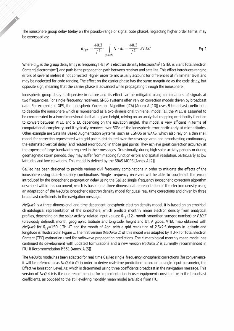
the ionosphere group delay (delay on the pseudo-range or signal code phase), neglecting higher order terms, may be expressed as:

where dIgr is the group delay [m], f is frequency [hz], N is electron density [electrons/m3], stec is slant total electron content [electrons/m2], and path is the propagation path between receiver and satellite. This effect introduces ranging errors of several meters if not corrected. higher order terms usually account for differences at millimeter level and may be neglected for code ranging. The effect on the carrier phase has the same magnitude as the code delay, but opposite sign, meaning that the carrier phase is advanced while propagating through the ionosphere.

ionospheric group delay is dispersive in nature and its effect can be mitigated using combinations of signals at two frequencies. For single-frequency receivers, GnSS systems often rely on correction models driven by broadcast data. For example, in GpS, the ionospheric correction algorithm (ica) [annex a [10]] uses 8 broadcast coefficients to describe the ionosphere which is represented as a two-dimensional thin-shell model (all the vTEc is assumed to be concentrated in a two-dimensional shell at a given height, relying on an analytical mapping or obliquity function to convert between vTEc and STEc depending on the elevation angle). This model is very efficient in terms of computational complexity and it typically removes over 50% of the ionospheric error particularly at mid-latitudes. other example are satellite based Augmentation systems, such as egnos or wAAs, which also rely on a thin shell model for correction represented with grid points distributed over the coverage area and broadcasting continuously the estimated vertical delay (and related error bound) in those grid points. they achieve great correction accuracy at the expense of large bandwidth required in their messages. occasionally, during high solar activity periods or during geomagnetic storm periods, they may suffer from mapping function errors and spatial resolution, particularly at low latitudes and low elevations. This model is defined by the SbaS mopS [annex a [2]].

Galileo has been designed to provide various civil frequency combinations in order to mitigate the effects of the ionosphere using dual-frequency combinations. single frequency receivers will be able to counteract the errors introduced by the ionospheric propagation delay using the galileo single-frequency ionospheric correction algorithm described within this document, which is based on a three dimensional representation of the electron density using an adaptation of the NeQuick ionospheric electron density model for quasi-real-time corrections and driven by three broadcast coefficients in the navigation message.

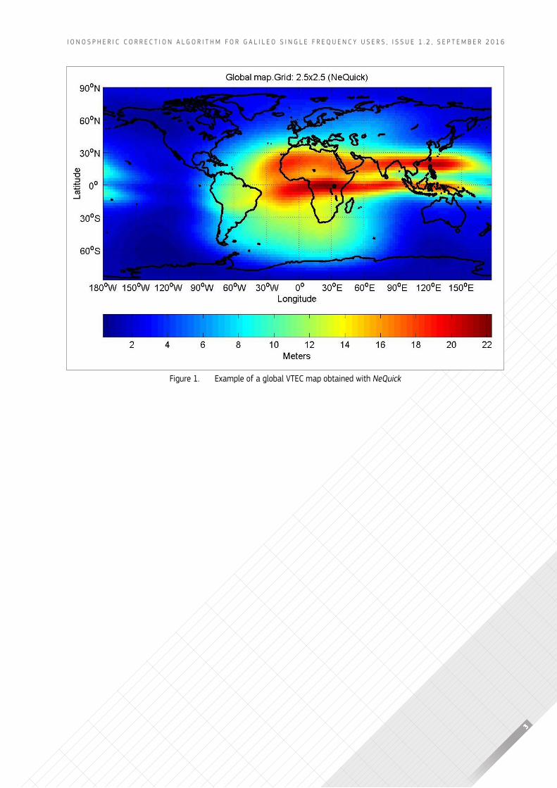
NeQuick is a three-dimensional and time dependent ionospheric electron density model. It is based on an empirical climatological representation of the ionosphere, which predicts monthly mean electron density from analytical profiles, depending on the solar activity-related input values: R12 (12 – month smoothed sunspot number) or F10�7 (previously defined), month, geographic latitude and longitude, height and uT. a global vTEc map obtained with NeQuick for R12=150, 13h ut and the month of April with a grid resolution of 2.5x2.5 degrees in latitude and longitude is illustrated in Figure 1. The first version (NeQuick 1) of this model was adapted by Itu-r for total electron content (tec) estimation used for radiowave propagation predictions. the climatological monthly mean model has continued its development with updated formulations and a new version NeQuick 2 is currently recommended in Itu-r recommendation p.531 [Annex A [3]].

the NeQuick model has been adapted for real-time galileo single-frequency ionospheric corrections (for convenience, it will be referred to as NeQuick G) in order to derive real-time predictions based on a single input parameter, the Effective ionisation level, Az, which is determined using three coefficients broadcast in the navigation message. This version of NeQuick is the one recommended for implementation in user equipment consistent with the broadcast coefficients, as opposed to the still evolving monthly mean model available from iTu.

𝑑𝑑𝐼𝐼𝐼𝐼𝐼𝐼 =40.3𝑓𝑓2 ∙ ∫ 𝑁𝑁 ∙ 𝑑𝑑𝑑𝑑

𝑝𝑝𝑝𝑝𝑝𝑝ℎ= 40.3

𝑓𝑓2 ∙ 𝑆𝑆𝑆𝑆𝑆𝑆𝑆𝑆 eq. 1

figure 1. Example of a global vTEc map obtained with NeQuick

3


the ionosphere group delay (delay on the pseudo-range or signal code phase), neglecting higher order terms, may be expressed as:

where dIgr is the group delay [m], f is frequency [hz], N is electron density [electrons/m3], stec is slant total electron content [electrons/m2], and path is the propagation path between receiver and satellite. This effect introduces ranging errors of several meters if not corrected. higher order terms usually account for differences at millimeter level and may be neglected for code ranging. The effect on the carrier phase has the same magnitude as the code delay, but opposite sign, meaning that the carrier phase is advanced while propagating through the ionosphere.

ionospheric group delay is dispersive in nature and its effect can be mitigated using combinations of signals at two frequencies. For single-frequency receivers, GnSS systems often rely on correction models driven by broadcast data. For example, in GpS, the ionospheric correction algorithm (ica) [annex a [10]] uses 8 broadcast coefficients to describe the ionosphere which is represented as a two-dimensional thin-shell model (all the vTEc is assumed to be concentrated in a two-dimensional shell at a given height, relying on an analytical mapping or obliquity function to convert between vTEc and STEc depending on the elevation angle). This model is very efficient in terms of computational complexity and it typically removes over 50% of the ionospheric error particularly at mid-latitudes. other example are satellite based Augmentation systems, such as egnos or wAAs, which also rely on a thin shell model for correction represented with grid points distributed over the coverage area and broadcasting continuously the estimated vertical delay (and related error bound) in those grid points. they achieve great correction accuracy at the expense of large bandwidth required in their messages. occasionally, during high solar activity periods or during geomagnetic storm periods, they may suffer from mapping function errors and spatial resolution, particularly at low latitudes and low elevations. This model is defined by the SbaS mopS [annex a [2]].

Galileo has been designed to provide various civil frequency combinations in order to mitigate the effects of the ionosphere using dual-frequency combinations. single frequency receivers will be able to counteract the errors introduced by the ionospheric propagation delay using the galileo single-frequency ionospheric correction algorithm described within this document, which is based on a three dimensional representation of the electron density using an adaptation of the NeQuick ionospheric electron density model for quasi-real-time corrections and driven by three broadcast coefficients in the navigation message.

NeQuick is a three-dimensional and time dependent ionospheric electron density model. It is based on an empirical climatological representation of the ionosphere, which predicts monthly mean electron density from analytical profiles, depending on the solar activity-related input values: R12 (12 – month smoothed sunspot number) or F10�7 (previously defined), month, geographic latitude and longitude, height and uT. a global vTEc map obtained with NeQuick for R12=150, 13h ut and the month of April with a grid resolution of 2.5x2.5 degrees in latitude and longitude is illustrated in Figure 1. The first version (NeQuick 1) of this model was adapted by Itu-r for total electron content (tec) estimation used for radiowave propagation predictions. the climatological monthly mean model has continued its development with updated formulations and a new version NeQuick 2 is currently recommended in Itu-r recommendation p.531 [Annex A [3]].

the NeQuick model has been adapted for real-time galileo single-frequency ionospheric corrections (for convenience, it will be referred to as NeQuick G) in order to derive real-time predictions based on a single input parameter, the Effective ionisation level, Az, which is determined using three coefficients broadcast in the navigation message. This version of NeQuick is the one recommended for implementation in user equipment consistent with the broadcast coefficients, as opposed to the still evolving monthly mean model available from iTu.

𝑑𝑑𝐼𝐼𝐼𝐼𝐼𝐼 =40.3𝑓𝑓2 ∙ ∫ 𝑁𝑁 ∙ 𝑑𝑑𝑑𝑑

𝑝𝑝𝑝𝑝𝑝𝑝ℎ= 40.3

𝑓𝑓2 ∙ 𝑆𝑆𝑆𝑆𝑆𝑆𝑆𝑆 eq. 1

figure 1. Example of a global vTEc map obtained with NeQuick

SECTION 2: SINglE FrEquENCy IONOSphErIC COrrECTION algOrIThm

5


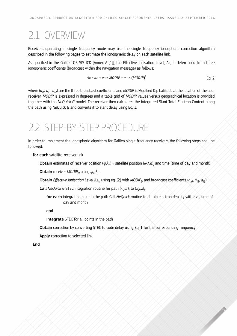
2.1 OvERvIEwreceivers operating in single frequency mode may use the single frequency ionospheric correction algorithm described in the following pages to estimate the ionospheric delay on each satellite link.

as specified in the Galileo oS SiS icD [annex a [1]], the Effective ionisation level, az, is determined from three ionospheric coefficients (broadcast within the navigation message) as follows:

where (ai0, ai1, ai2) are the three broadcast coefficients and MODiP is modified Dip latitude at the location of the user receiver. MODiP is expressed in degrees and a table grid of MODiP values versus geographical location is provided together with the NeQuick G model. the receiver then calculates the integrated slant total electron content along the path using NeQuick G and converts it to slant delay using eq. 1.

2.2 Step-by-Step procedureIn order to implement the ionospheric algorithm for galileo single frequency receivers the following steps shall be followed:

for each satellite-receiver link

Obtain estimates of receiver position (φ,λ,h)i, satellite position (φ,λ,h)j and time (time of day and month)

Obtain receiver MODiPu using φi, λi.

Obtain Effective Ionisation Level AzU using eq. (2) with MODiPu and broadcast coefficients (ai0, ai1, ai2)

Call NeQuick G stec integration routine for path (x,y,z)i to (x,y,z)j,

for each integration point in the path call NeQuick routine to obtain electron density with AzU, time of day and month

end

Integrate stec for all points in the path

Obtain correction by converting stec to code delay using eq. 1 for the corresponding frequency

Apply correction to selected link

End

Az = ai0 + ai1 × MODIP + ai2 × (MODIP)2 eq. 2

6

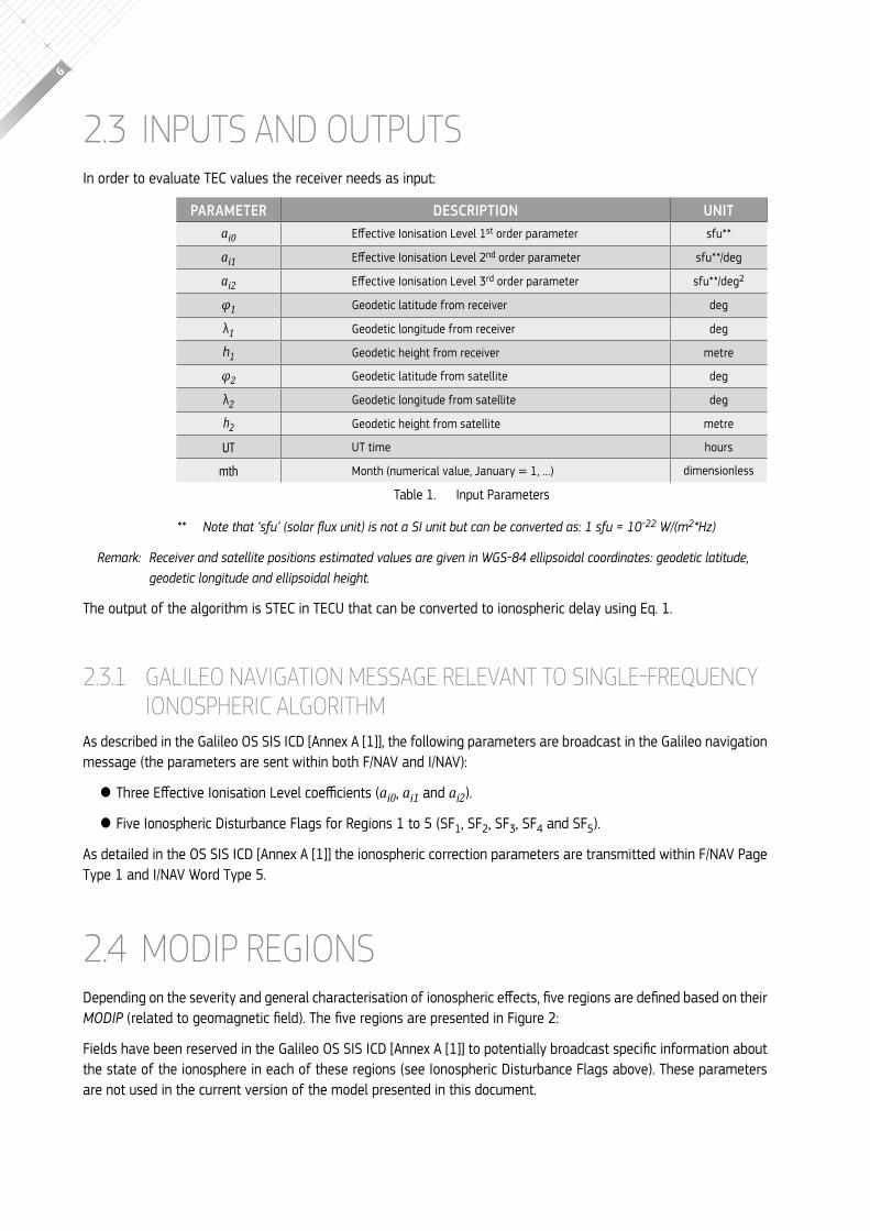
2.3 INpUTS AND OUTpUTS In order to evaluate tec values the receiver needs as input:

** Note that ‘sfu’ (solar flux unit) is not a SI unit but can be converted as: 1 sfu = 10-22 W/(m2*Hz)

Remark: Receiver and satellite positions estimated values are given in WGS-84 ellipsoidal coordinates: geodetic latitude, geodetic longitude and ellipsoidal height�

the output of the algorithm is stec in tecu that can be converted to ionospheric delay using eq. 1.

2.3.1 Galileo naviGation meSSaGe relevant to SinGle-frequency IONOSphERIC ALgORIThM

As described in the galileo os sIs IcD [Annex A [1]], the following parameters are broadcast in the galileo navigation message (the parameters are sent within both F/nav and i/nav):

● Three Effective ionisation level coefficients (ai0, ai1 and ai2).

● five Ionospheric Disturbance flags for regions 1 to 5 (sf1, sf2, sf3, sf4 and sf5).

as detailed in the oS SiS icD [annex a [1]] the ionospheric correction parameters are transmitted within F/nav page Type 1 and i/nav word Type 5.

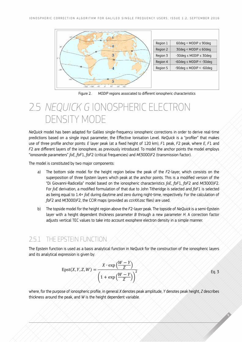
2.4 MODIp REgIONSDepending on the severity and general characterisation of ionospheric effects, five regions are defined based on their MODiP (related to geomagnetic field). The five regions are presented in Figure 2:

Fields have been reserved in the Galileo oS SiS icD [annex a [1]] to potentially broadcast specific information about the state of the ionosphere in each of these regions (see Ionospheric Disturbance flags above). these parameters are not used in the current version of the model presented in this document.

PARAmEtER DESCRIPtION UNItai0 Effective ionisation level 1st order parameter sfu**

ai1 Effective ionisation level 2nd order parameter sfu**/deg

ai2 Effective ionisation level 3rd order parameter sfu**/deg2

φ1 geodetic latitude from receiver deg

λ1 geodetic longitude from receiver deg

h1 geodetic height from receiver metre

φ2 geodetic latitude from satellite deg

λ2 geodetic longitude from satellite deg

h2 geodetic height from satellite metre

UT ut time hours

mth month (numerical value, january = 1, …) dimensionless

table 1. Input parameters

region 1 60deg < moDip ≤ 90deg


region 3 -30deg ≤ moDip ≤ 30deg

region 4 -60deg ≤ moDip < -30deg


figure 2. MODiP regions associated to different ionospheric characteristics

7


2.3 INpUTS AND OUTpUTS In order to evaluate tec values the receiver needs as input:

** Note that ‘sfu’ (solar flux unit) is not a SI unit but can be converted as: 1 sfu = 10-22 W/(m2*Hz)

Remark: Receiver and satellite positions estimated values are given in WGS-84 ellipsoidal coordinates: geodetic latitude, geodetic longitude and ellipsoidal height�

the output of the algorithm is stec in tecu that can be converted to ionospheric delay using eq. 1.

2.3.1 Galileo naviGation meSSaGe relevant to SinGle-frequency IONOSphERIC ALgORIThM

As described in the galileo os sIs IcD [Annex A [1]], the following parameters are broadcast in the galileo navigation message (the parameters are sent within both F/nav and i/nav):

● Three Effective ionisation level coefficients (ai0, ai1 and ai2).

● five Ionospheric Disturbance flags for regions 1 to 5 (sf1, sf2, sf3, sf4 and sf5).

as detailed in the oS SiS icD [annex a [1]] the ionospheric correction parameters are transmitted within F/nav page Type 1 and i/nav word Type 5.

2.4 MODIp REgIONSDepending on the severity and general characterisation of ionospheric effects, five regions are defined based on their MODiP (related to geomagnetic field). The five regions are presented in Figure 2:

Fields have been reserved in the Galileo oS SiS icD [annex a [1]] to potentially broadcast specific information about the state of the ionosphere in each of these regions (see Ionospheric Disturbance flags above). these parameters are not used in the current version of the model presented in this document.

PARAmEtER DESCRIPtION UNItai0 Effective ionisation level 1st order parameter sfu**

ai1 Effective ionisation level 2nd order parameter sfu**/deg

ai2 Effective ionisation level 3rd order parameter sfu**/deg2

φ1 geodetic latitude from receiver deg

λ1 geodetic longitude from receiver deg

h1 geodetic height from receiver metre

φ2 geodetic latitude from satellite deg

λ2 geodetic longitude from satellite deg

h2 geodetic height from satellite metre

UT ut time hours

mth month (numerical value, january = 1, …) dimensionless

table 1. Input parameters



region 3 -30deg ≤ moDip ≤ 30deg



figure 2. MODiP regions associated to different ionospheric characteristics

2.5 NeQuick G IONOSphERIC ELECTRON denSity mode

NeQuick model has been adapted for galileo single-frequency ionospheric corrections in order to derive real-time predictions based on a single input parameter, the Effective ionisation level. NeQuick is a “profiler” that makes use of three profile anchor points: e layer peak (at a fixed height of 120 km), F1 peak, F2 peak, where e, F1 and F2 are different layers of the ionosphere, as previously introduced. To model the anchor points the model employs “ionosonde parameters” foe, foF1, foF2 (critical frequencies) and M(3000)F2 (transmission factor).

the model is constituted by two major components:

a) the bottom side model for the height region below the peak of the F2-layer, which consists on the superposition of three Epstein layers which peak at the anchor points. This is a modified version of the “Di giovanni-radicella” model based on the ionospheric characteristics foe, foF1, foF2 and M(3000)F2. for foe derivation, a modified formulation of that due to John Titheridge is selected and foF1 is selected as being equal to 1.4× foe during daytime and zero during night-time, respectively. for the calculation of foF2 and M(3000)F2, the ccIr maps (provided as ccirXX�asc files) are used.

b) the topside model for the height region above the F2-layer peak. the topside of NeQuick is a semi-epstein layer with a height dependent thickness parameter B through a new parameter H. A correction factor adjusts vertical tec values to take into account exosphere electron density in a simple manner.

2.5.1 ThE EpSTEIN FUNCTIONthe epstein function is used as a basis analytical function in NeQuick for the construction of the ionospheric layers and its analytical expression is given by:

where, for the purpose of ionospheric profile, in general X denotes peak amplitude, Y denotes peak height, Z describes thickness around the peak, and W is the height dependent variable.

Epst(𝑋𝑋, 𝑌𝑌, 𝑍𝑍,𝑊𝑊) =𝑋𝑋 ∙ exp (𝑊𝑊 − 𝑌𝑌

𝑍𝑍 )

(1 + exp (𝑊𝑊 − 𝑌𝑌𝑍𝑍 ))

2 eq. 3

8

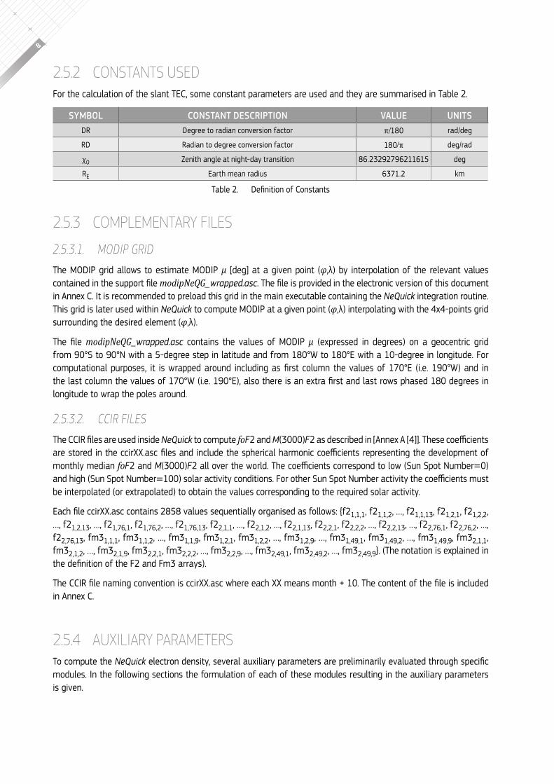
2.5.2 CONSTANTS USEDfor the calculation of the slant tec, some constant parameters are used and they are summarised in table 2.

2.5.3 complementary fileS

2.5.3.1. MODiP GriDthe moDIp grid allows to estimate moDIp μ [deg] at a given point (φ,λ) by interpolation of the relevant values contained in the support file modipNeQG_wrapped.asc. The file is provided in the electronic version of this document in Annex c. It is recommended to preload this grid in the main executable containing the NeQuick integration routine. this grid is later used within NeQuick to compute moDIp at a given point (φ,λ) interpolating with the 4x4-points grid surrounding the desired element (φ,λ).

The file modipNeQG_wrapped.asc contains the values of moDIp μ (expressed in degrees) on a geocentric grid from 90°s to 90°n with a 5-degree step in latitude and from 180°w to 180°e with a 10-degree in longitude. for computational purposes, it is wrapped around including as first column the values of 170°E (i.e. 190°w) and in the last column the values of 170°w (i.e. 190°E), also there is an extra first and last rows phased 180 degrees in longitude to wrap the poles around.

2.5.3.2. ccir files The ccir files are used inside NeQuick to compute foF2 and M(3000)F2 as described in [annex a [4]]. These coefficients are stored in the ccirxx.asc files and include the spherical harmonic coefficients representing the development of monthly median foF2 and M(3000)F2 all over the world. The coefficients correspond to low (Sun Spot number=0) and high (sun spot number=100) solar activity conditions. For other Sun Spot number activity the coefficients must be interpolated (or extrapolated) to obtain the values corresponding to the required solar activity.

Each file ccirxx.asc contains 2858 values sequentially organised as follows: {f21,1,1, f21,1,2, …, f21,1,13, f21,2,1, f21,2,2, …, f21,2,13, …, f21,76,1, f21,76,2, …, f21,76,13, f22,1,1, …, f22,1,2, …, f22,1,13, f22,2,1, f22,2,2, …, f22,2,13, …, f22,76,1, f22,76,2, …, f22,76,13, fm31,1,1, fm31,1,2, …, fm31,1,9, fm31,2,1, fm31,2,2, …, fm31,2,9, …, fm31,49,1, fm31,49,2, …, fm31,49,9, fm32,1,1, fm32,1,2, …, fm32,1,9, fm32,2,1, fm32,2,2, …, fm32,2,9, …, fm32,49,1, fm32,49,2, …, fm32,49,9}. (the notation is explained in the definition of the F2 and Fm3 arrays).

The ccir file naming convention is ccirxx.asc where each xx means month + 10. The content of the file is included in Annex c.

2.5.4 auxiliary parameterSto compute the NeQuick electron density, several auxiliary parameters are preliminarily evaluated through specific modules. In the following sections the formulation of each of these modules resulting in the auxiliary parameters is given.

SymbOl CONStANt DESCRIPtION vAlUE UNItSDr Degree to radian conversion factor π ⁄180 rad/deg

rD radian to degree conversion factor 180⁄π deg/rad

χ0 zenith angle at night-day transition 86.23292796211615 deg

re earth mean radius 6371.2 km

table 2. Definition of constants

9


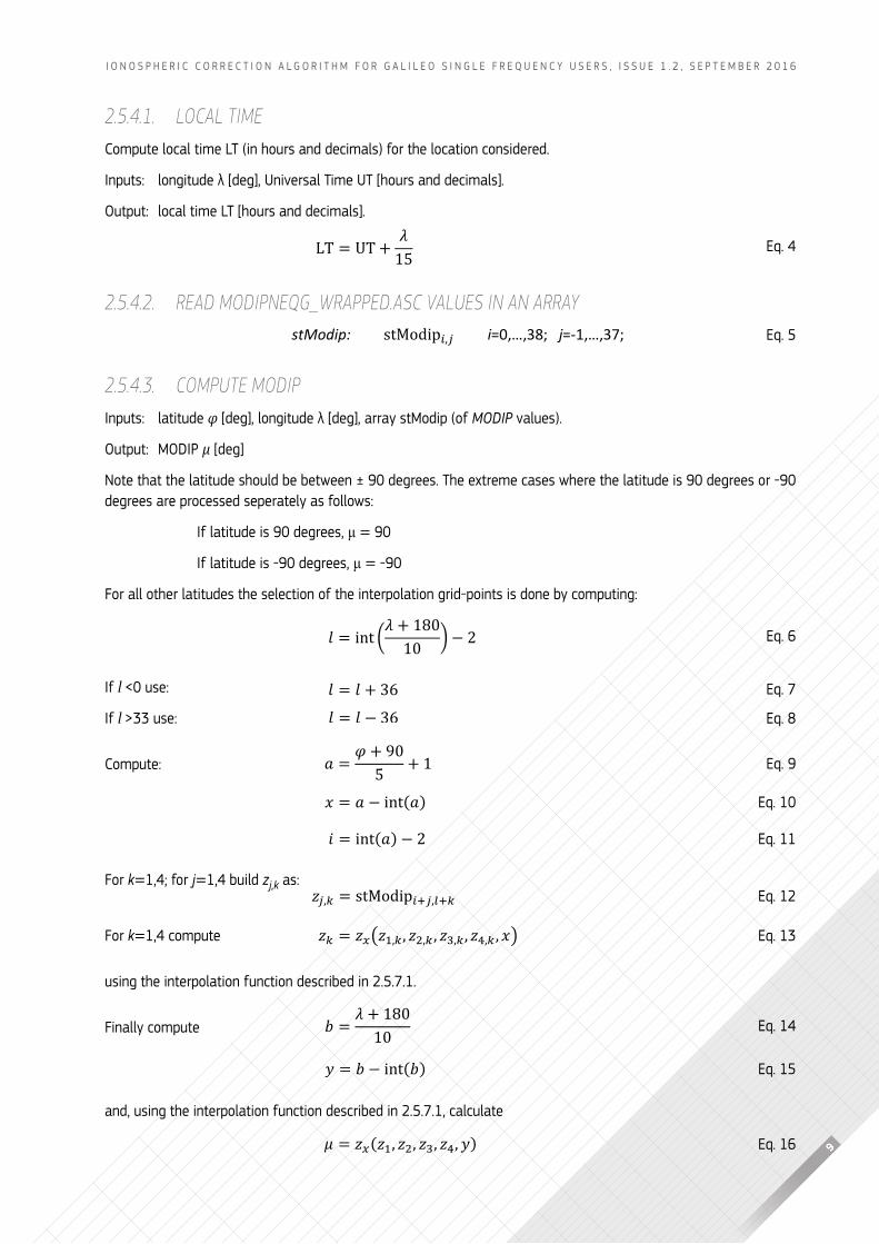
2.5.4.1. lOcal TiMecompute local time lt (in hours and decimals) for the location considered.

inputs: longitude λ [deg], universal Time uT [hours and decimals].

output: local time lt [hours and decimals].

2.5.4.2. reaD MODiPNeQG_wraPPeD.asc values iN aN array

2.5.4.3. cOMPuTe MODiPInputs: latitude φ [deg], longitude λ [deg], array stmodip (of MODiP values).

output: moDIp μ [deg]

note that the latitude should be between ± 90 degrees. the extreme cases where the latitude is 90 degrees or -90 degrees are processed seperately as follows:

If latitude is 90 degrees, μ = 90

If latitude is -90 degrees, μ = -90

for all other latitudes the selection of the interpolation grid-points is done by computing:

If l <0 use:

If l >33 use:

compute:

for k=1,4; for j=1,4 build zj,k as:

for k=1,4 compute

using the interpolation function described in 2.5.7.1.

finally compute

and, using the interpolation function described in 2.5.7.1, calculate

LT = UT + 𝜆𝜆15 eq. 4

stModip: stModip𝑖𝑖,𝑗𝑗 i=0,…,38; j=-1,…,37; eq. 5

𝑙𝑙 = int (𝜆𝜆 + 18010 ) − 2 eq. 6

𝑙𝑙 = 𝑙𝑙 + 36 eq. 7

𝑙𝑙 = 𝑙𝑙 − 36 eq. 8

𝑎𝑎 = 𝜑𝜑 + 905 + 1 eq. 9

𝑥𝑥 = 𝑎𝑎 − int(𝑎𝑎) eq. 10

𝑖𝑖 = int(𝑎𝑎) − 2 eq. 11

eq. 12 𝑧𝑧𝑗𝑗,𝑘𝑘 = stModip𝑖𝑖+𝑗𝑗,𝑙𝑙+𝑘𝑘

eq. 13 𝑧𝑧𝑘𝑘 = 𝑧𝑧𝑥𝑥(𝑧𝑧1,𝑘𝑘, 𝑧𝑧2,𝑘𝑘, 𝑧𝑧3,𝑘𝑘, 𝑧𝑧4,𝑘𝑘, 𝑥𝑥)

eq. 14 𝑏𝑏 = 𝜆𝜆 + 18010

eq. 15 𝑦𝑦 = 𝑏𝑏 − int(𝑏𝑏)

𝜇𝜇 = 𝑧𝑧𝑥𝑥(𝑧𝑧1, 𝑧𝑧2, 𝑧𝑧3, 𝑧𝑧4, 𝑦𝑦) eq. 16

10

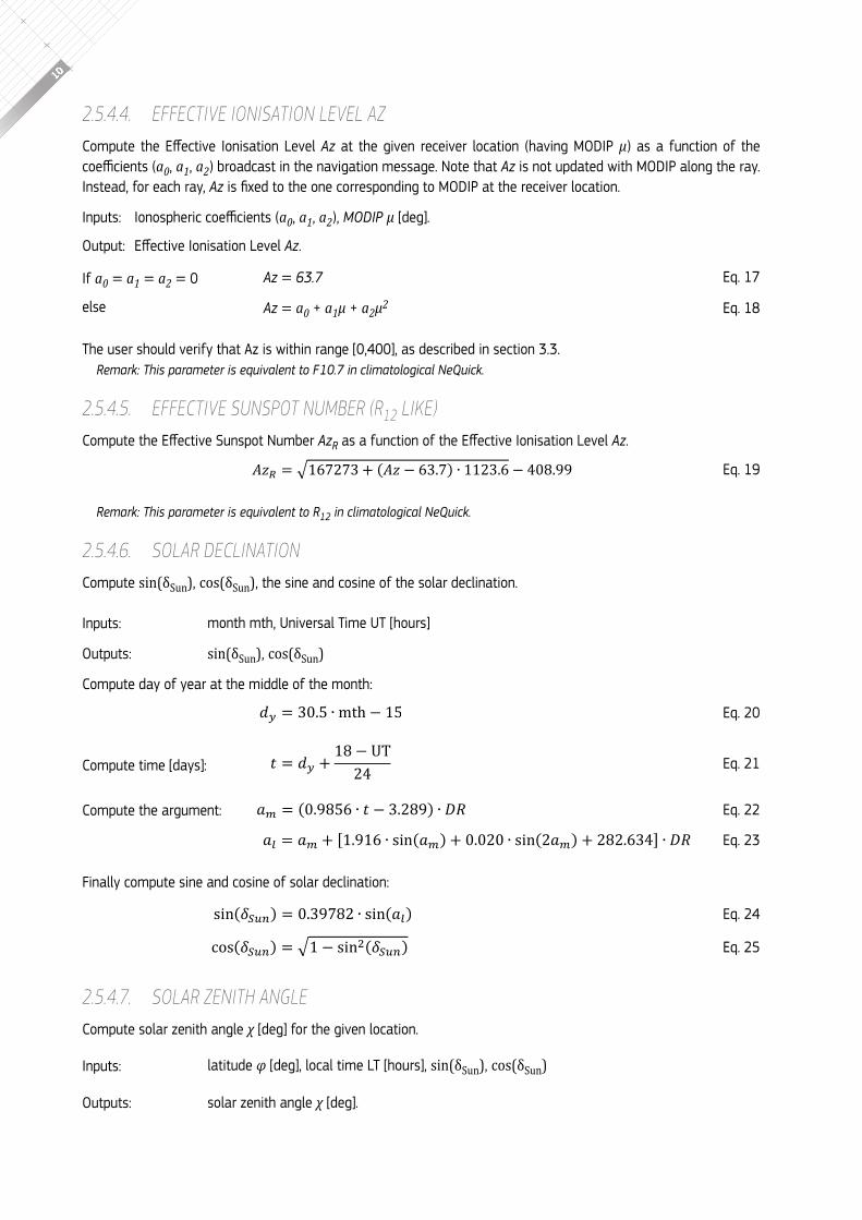
2.5.4.4. effecTive iONisaTiON level azcompute the Effective ionisation level Az at the given receiver location (having moDIp μ) as a function of the coefficients (a0, a1, a2) broadcast in the navigation message. note that Az is not updated with moDIp along the ray. Instead, for each ray, Az is fixed to the one corresponding to moDip at the receiver location.

inputs: ionospheric coefficients (a0, a1, a2), MODiP μ [deg].

output: Effective ionisation level Az.

If a0 = a1 = a2 = 0

else

the user should verify that Az is within range [0,400], as described in section 3.3.Remark: This parameter is equivalent to F10.7 in climatological NeQuick.

2.5.4.5. EffEctivE SunSpot numbEr (r12 likE)compute the Effective Sunspot number AzR as a function of the Effective ionisation level Az.

Remark: This parameter is equivalent to R12 in climatological NeQuick�

2.5.4.6. sOlar DecliNaTiONcompute sin(δSun), cos(δSun), the sine and cosine of the solar declination.

Inputs:

outputs:

compute day of year at the middle of the month:

compute time [days]:

compute the argument:

finally compute sine and cosine of solar declination:

2.5.4.7. sOlar zeNiTh aNGlecompute solar zenith angle χ [deg] for the given location.

Inputs:

outputs:

Az = 63�7 eq. 17

Az = a0 + a1μ + a2μ2 eq. 18

𝐴𝐴𝐴𝐴𝑅𝑅 = √167273 + (𝐴𝐴𝐴𝐴 − 63.7) ∙ 1123.6 − 408.99 eq. 19

month mth, universal time ut [hours]

sin(δSun), cos(δSun)

𝑑𝑑𝑦𝑦 = 30.5 ∙ mth − 15 eq. 20

𝑡𝑡 = 𝑑𝑑𝑦𝑦 +18 − UT24 eq. 21

𝑎𝑎𝑚𝑚 = (0.9856 ∙ 𝑡𝑡 − 3.289) ∙ 𝐷𝐷𝐷𝐷 eq. 22

𝑎𝑎𝑙𝑙 = 𝑎𝑎𝑚𝑚 + [1.916 ∙ sin(𝑎𝑎𝑚𝑚) + 0.020 ∙ sin(2𝑎𝑎𝑚𝑚) + 282.634] ∙ 𝐷𝐷𝐷𝐷 eq. 23

sin(𝛿𝛿𝑆𝑆𝑆𝑆𝑆𝑆) = 0.39782 ∙ sin(𝑎𝑎𝑙𝑙) eq. 24

cos(𝛿𝛿𝑆𝑆𝑆𝑆𝑆𝑆) = √1 − sin2(𝛿𝛿𝑆𝑆𝑆𝑆𝑆𝑆) eq. 25

latitude φ [deg], local time lt [hours], sin(δSun), cos(δSun)

solar zenith angle χ [deg].

11


compute

2.5.4.8. effecTive sOlar zeNiTh aNGlecompute the effective solar zenith angle χeff [deg] as a function of the solar zenith angle χ [deg] and the solar zenith angle at day night transition χ0 [deg].

Inputs:

output:

set

then

2.5.5 MODEL pARAMETERSIn the following sections model peak parameter and auxiliary parameter values are calculated.

2.5.5.1. foe aND Nmeto compute the e layer critical frequency foe [mhz] at a given location, in addition to the effective solar zenith angle χeff, a season dependent parameter has to be computed.

Inputs:

output:

Define the seas parameter as a function of the month of the year as follows:

Introduce the latitudinal dependence:

cos(𝜒𝜒) = sin(𝜑𝜑 ∙ 𝐷𝐷𝐷𝐷) ∙ sin(𝛿𝛿𝑆𝑆𝑆𝑆𝑆𝑆) + cos(𝜑𝜑 ∙ 𝐷𝐷𝐷𝐷) ∙ cos(𝛿𝛿𝑆𝑆𝑆𝑆𝑆𝑆) ∙ cos (𝜋𝜋12 (12 − 𝐿𝐿𝐿𝐿)) eq. 26

𝜒𝜒 = 𝑅𝑅𝑅𝑅 ∙ atan2 (√1 − cos2(𝜒𝜒) , cos(𝜒𝜒)) eq. 27

solar zenith angle χ [deg], χ0 [deg]

effective solar zenith angle χeff [deg].

χ0 = 86.23292796211615° eq. 28

𝜒𝜒𝑒𝑒𝑒𝑒𝑒𝑒 = 𝜒𝜒 + [90 − 0.24 ∙ exp(20 − 0.2 ∙ 𝜒𝜒)] ∙ exp(12(𝜒𝜒 − 𝜒𝜒0))1 + exp(12(𝜒𝜒 − 𝜒𝜒0))

eq. 29

latitude φ [deg], Effective ionisation level Az,

effective solar zenith angle χeff [deg], month mth.

foe [mhz].

Nme [1011 m-3]

eq. 31

eq. 32

If mth = 1,2,11,12 then seas = -1

If mth = 3,4,9,10 then seas = 0

if mth = 5,6,7,8 then seas = 1

eq. 30

𝑒𝑒𝑒𝑒 = exp(0.3 ∙ 𝜑𝜑) eq. 33

𝑠𝑠𝑠𝑠𝑠𝑠𝑠𝑠𝑠𝑠 = 𝑠𝑠𝑠𝑠𝑠𝑠𝑠𝑠 ∙ 𝑠𝑠𝑠𝑠 − 1𝑠𝑠𝑠𝑠 + 1 eq. 34

𝑓𝑓𝑓𝑓𝑓𝑓 = √(1.112 − 0.019 ∙ 𝑠𝑠𝑠𝑠𝑠𝑠𝑠𝑠𝑠𝑠)2 ∙ √𝐴𝐴𝐴𝐴 ∙ [cos(𝜒𝜒𝑒𝑒𝑒𝑒𝑒𝑒 ∙ 𝐷𝐷𝐷𝐷)]0.6 + 0.49 eq. 35

12

the e layer maximum density Nme [1011 m-3] as a function of foe [mhz] is computed as:

2.5.5.2. fof1 aND Nmf1the F1 layer critical frequency foF1 [mhz] is computed as:

Inputs:

outputs:

Note: The implementation of this calculation in Annex F takes into account the need to ensure continuity and derivability over the full range of f0F1, by making use of the NeqJoin function defined in F.2.12.1.

the F1 layer maximum density NmF1 [1011 m-3] as a function of foF1 [mhz] is computed as:

2.5.5.3. fof2 aND Nmf2; m(3000)f2

2.5.5.3.1. READ CcirXX.Asc vALUES

Input: month mth

outputs F2, Fm3

Select the file name to read: XX = mth + 10

(e.g. ccir21.asc for november) and store the file content in the two arrays of coefficients:

coefficients for fof2

F2: f 2i,j,k i=1,2; j=1,…,76; k=1,…,13

coefficients for M(3000)F2

Fm3: fm3i,j,k i=1,2; j=1,…,49; k=1,…,9

2.5.5.3.2. interpolate itu-r coefficientS for azr

compute AF2, the array of interpolated coefficients for foF2 and Am3, the array of interpolated coefficients for M(3000)F2

Inputs: F2, Fm3, AzR

outputs: AF2, Am3

𝑁𝑁𝑁𝑁𝑁𝑁 = 0.124 ∙ 𝑓𝑓𝑓𝑓𝑁𝑁2 eq. 36

e layer critical frequency foe [mhz], fof2 [mhz]

foF1 = 1.4* foe if foe ≥ 2.0 mhz,

foF1 = 0 if foe < 2.0 mhz,

foF1 is reduced by 15% if too close to foF2

if foF1 < 10-6 then foF1 = 0

eq. 37

foF1 [mhz], NmF1 [1011 m-3]

𝑁𝑁𝑁𝑁𝑁𝑁1 = 0.124 ∙ (𝑓𝑓𝑓𝑓𝑓𝑓 + 0.5)2 if foF1 ≤ 0 and foe > 2 eq. 38

𝑁𝑁𝑁𝑁𝑁𝑁1 = 0.124 ∙ 𝑓𝑓𝑓𝑓𝑁𝑁12 otherwise eq. 39

eq. 40

eq. 41

eq. 42

13


compute the array of interpolated coefficients for foF2

Af2: af2j,k j=1,…,76; k=1,…,13

AF2 elements are calculated by linear combination of the elements of F2:

compute the array of interpolated coefficients for M(3000)F2:

Am3: am3j,k j=1,…,49; k=1,…,9

Am3 elements are calculated by linear combination of the elements of Fm3:

2.5.5.3.3. COMpUTE FOURIER TIME SERIES FOR fof2 AND M(3000)f2

inputs: universal Time uT [hours], arrays of interpolated iTu-r coefficients AF2, Am3

outputs: cF2, cm3, vectors of coefficients for legendre calculation for foF2 and M(3000)F2

the vector cf2 has 76 elements:

the vector cm3 has 49 elements:

compute the time argument:

T = ( 15∙UT-180) • DR

for i=1,..,76 calculate the fourier time series for foF2:

for i=1,..,49 calculate the fourier time series for M(3000)F2:

2.5.5.3.4. COMpUTE fof2 AND M(3000)f2 by leGendre calculation

Inputs:

outputs:

eq. 43

𝑎𝑎𝑎𝑎2𝑗𝑗,𝑘𝑘 = 𝑎𝑎21,𝑗𝑗,𝑘𝑘 (1 −𝐴𝐴𝐴𝐴𝑅𝑅100) + 𝑎𝑎22,𝑗𝑗,𝑘𝑘

𝐴𝐴𝐴𝐴𝑅𝑅100 j=1,…,76; k=1,…,13 eq. 44

eq. 45

𝑎𝑎𝑎𝑎3𝑗𝑗,𝑘𝑘 = 𝑓𝑓𝑎𝑎31,𝑗𝑗,𝑘𝑘 (1 −𝐴𝐴𝐴𝐴𝑅𝑅100) + 𝑓𝑓𝑎𝑎32,𝑗𝑗,𝑘𝑘

𝐴𝐴𝐴𝐴𝑅𝑅100 j=1,…,49; k=1,…,9 eq. 46

cF2: cf 2l l=1,…,76 eq. 47

cm3: cm3l l=1,…,49 eq. 48

eq. 49

𝑐𝑐𝑐𝑐2𝑖𝑖 = 𝑎𝑎𝑐𝑐2𝑖𝑖,1 +∑[𝑎𝑎𝑐𝑐2𝑖𝑖,2𝑘𝑘 sin(𝑘𝑘𝑘𝑘) + 𝑎𝑎𝑐𝑐2𝑖𝑖,2𝑘𝑘+1 cos(𝑘𝑘𝑘𝑘)]6

𝑘𝑘=1 eq. 50

eq. 51 𝑐𝑐𝑐𝑐3𝑖𝑖 = 𝑎𝑎𝑐𝑐3𝑖𝑖,1 +∑[𝑎𝑎𝑐𝑐3𝑖𝑖,2𝑘𝑘 sin(𝑘𝑘𝑘𝑘) + 𝑎𝑎𝑐𝑐3𝑖𝑖,2𝑘𝑘+1 cos(𝑘𝑘𝑘𝑘)]4

𝑘𝑘=1

moDIp μ [deg], latitude φ [deg], longitude λ [deg], vector cF2 of the coefficients for legendre combination for foF2, vector cm3 of the coefficients for legendre combination for M(3000)F2

foF2 [mhz], M(3000)F2

14

Define vectors containing sine and cosine of the coordinates:

Compute MODIP coefficientsm1 = 1

and for k=2,…,12

Compute latitude and longitude coefficients

for n=2,…,9

Compute foF2

order 0 term:

having the increased legendre grades for foF2 in a vector:

for computational efficiency, define also:

k: kn n = 1,...,9

k1 = –q1

and for n=2,…,9

for n=2,…,9 compute the higher order terms:

finally sum the terms to obtain foF2:

M: mk k = 1,…,12 eq. 52

P: pn n = 2,…,9 eq. 53

S: sn n = 2,…,9 eq. 54

C: cn n = 2,…,9 eq. 55

eq. 56

𝑚𝑚𝑘𝑘 = sin𝑘𝑘−1(𝜇𝜇 ∙ 𝐷𝐷𝐷𝐷) eq. 57

𝑝𝑝𝑛𝑛 = cos𝑛𝑛−1(𝜑𝜑 ∙ 𝐷𝐷𝐷𝐷) eq. 58

𝑠𝑠𝑛𝑛 = sin((𝑛𝑛 − 1) ∙ 𝜆𝜆 ∙ 𝐷𝐷𝐷𝐷) eq. 59

𝑐𝑐𝑛𝑛 = cos((𝑛𝑛 − 1) ∙ 𝜆𝜆 ∙ 𝐷𝐷𝐷𝐷) eq. 60

𝑓𝑓𝑓𝑓𝑓𝑓21 = ∑𝑐𝑐𝑓𝑓2𝑘𝑘𝑚𝑚𝑘𝑘

12

𝑘𝑘=1 eq. 61

Q: qn n = 1,…,9 eq. 62

Q = (12,12,9,5,2,1,1,1,1) eq. 63

eq. 64

eq. 65

𝑘𝑘𝑛𝑛 = 𝑘𝑘𝑛𝑛−1 + 2𝑞𝑞𝑛𝑛−1 eq. 66

𝑓𝑓𝑓𝑓𝑓𝑓2𝑛𝑛 = ∑(𝑐𝑐𝑓𝑓2𝑘𝑘𝑛𝑛+2𝑘𝑘−1𝑐𝑐𝑛𝑛 + 𝑐𝑐𝑓𝑓2𝑘𝑘𝑛𝑛+2𝑘𝑘𝑠𝑠𝑛𝑛)𝑚𝑚𝑘𝑘𝑝𝑝𝑛𝑛𝑞𝑞𝑛𝑛

𝑘𝑘=1 eq. 67

𝑓𝑓𝑓𝑓𝑓𝑓2 = ∑𝑓𝑓𝑓𝑓𝑓𝑓2𝑛𝑛9

𝑛𝑛=1 eq. 68

15


Compute M(3000)F2

order 0 term:

having the increased legendre grades for M(3000)F2 in a vector:

R: rn n = 1,…,7

R = (7,8,6,3,2,1,1)

for computational efficiency, define also:

H: hn n = 1,…,7

h1 = –r1

and for n=2,…,7

for n=2,…7, compute the higher order terms

finally sum the terms:

to compute NmF2 use:

where NmF2 is in [1011m-3].

2.5.5.4. hMethe e layer maximum density height hme [km] is defined as a constant:

hme = 120

2.5.5.5. hMf1compute the F1 layer maximum density height hmF1 [km]:

Inputs: hmF2 [km], hme [km]

output: hmF1 [km]

𝑀𝑀(3000)𝐹𝐹21 = �𝑐𝑐𝑐𝑐3𝑘𝑘𝑐𝑐𝑘𝑘

7

𝑘𝑘=1

eq. 69

eq. 70

eq. 71

eq. 72

eq. 73

ℎ𝑛𝑛 = ℎ𝑛𝑛−1 + 2𝑟𝑟𝑛𝑛−1 eq. 74

𝑀𝑀(3000)𝐹𝐹2𝑛𝑛 = ∑(𝑐𝑐𝑐𝑐3ℎ𝑛𝑛+2𝑘𝑘−1𝑐𝑐𝑛𝑛 + 𝑐𝑐𝑐𝑐3ℎ𝑛𝑛+2𝑘𝑘𝑠𝑠𝑛𝑛)𝑐𝑐𝑘𝑘𝑝𝑝𝑛𝑛𝑟𝑟𝑛𝑛

𝑘𝑘=1 eq. 75

𝑀𝑀(3000) = ∑𝑀𝑀(3000)𝐹𝐹2𝑛𝑛7

𝑛𝑛=1 eq. 76

𝑁𝑁𝑁𝑁𝑁𝑁2 = 0.124 ∙ 𝑓𝑓𝑓𝑓𝑁𝑁22 eq. 77

eq. 78

ℎ𝑚𝑚𝑚𝑚1 = ℎ𝑚𝑚𝑚𝑚2 + ℎ𝑚𝑚𝑚𝑚2 eq. 79

16

2.5.5.6. hMf2compute the F2 layer maximum density height hmF2 [km].

Inputs: foe [mhz], foF2 [mhz], M(3000)F2

output: hmF2 [km]

whereM = M(3000)F2

∆M = ― 0.012 if foE < 10-30

if foE ≥ 10-30

and the ratio ρ is computed as:

2.5.5.7. B2BOT, B1TOP, B1BOT, BeTOP, BeBOTcompute the thickness parameters B2bot, B1top, B1bot, Betop, Bebot [km]

2.5.5.8. a1compute the F2 layer amplitude A1 [1011 m-3].

Inputs: NmF2 [1011 m-3]

output: A1 [1011 m-3]

A1 = 4 • NmF2

ℎ𝑚𝑚𝑚𝑚2 =1490 ∙ 𝑀𝑀 ∙ √0.0196 ∙ 𝑀𝑀

2 + 11.2967 ∙ 𝑀𝑀2 − 1

𝑀𝑀 + ∆𝑀𝑀 − 176 eq. 80

eq. 81

eq. 82

∆𝑀𝑀 = 0.253𝜌𝜌 − 1.215 − 0.012 eq. 83

𝜌𝜌 =

𝑓𝑓𝑓𝑓𝑓𝑓2𝑓𝑓𝑓𝑓𝑓𝑓 ∙ exp(20 ∙ (𝑓𝑓𝑓𝑓𝑓𝑓2𝑓𝑓𝑓𝑓𝑓𝑓 − 1.75)) + 1.75

exp(20 ∙ (𝑓𝑓𝑓𝑓𝑓𝑓2𝑓𝑓𝑓𝑓𝑓𝑓 − 1.75)) + 1 eq. 84

𝐵𝐵2𝑏𝑏𝑏𝑏𝑏𝑏 = 0.385 ∙ 𝑁𝑁𝑁𝑁𝑁𝑁20.01 ∙ exp(−3.467 + 0.857 ∙ ln(𝑓𝑓𝑏𝑏𝑁𝑁22) + 2.02 ∙ ln(𝑀𝑀))

INPUtS OUtPUtS DEFINItION

NmF2 [1011 m-3]

foF2 [mhz]

M(3000)F2

B2bot [km]eq. 85

where M=M(3000)F2

hmF1 [km]

hmF2[km]B1top [km] B1top = 0.3 • (hmF2 ― hmF1) eq. 86

hmF1 [km]

hme [km]B1bot [km] B1bot = 0.5 • (hmF1 ― hmE) eq. 87

B1bot [km] Betop [km] BEtop = max[B1bot, 7] eq. 88

Bebot [km] BEbot = 5 eq. 89

eq. 90

17


2.5.5.9. a2 aND a3 compute the F1 layer amplitude A2 [1011 m-3] and the e layer amplitude A3 [1011 m-3].

Inputs: Nme [1011 m-3], NmF1 [1011 m-3], A1[1011 m-3], hmF2 [km], hmF1 [km], hme [km], Betop [km], B1bot [km], B2bot [km], foF1 [mhz]

output: A2 [1011 m-3], A3 [1011 m-3]

if foF1 < 0.5: A2 = 0

A3 = 4.0 • [NmE ― Epst(A1, hmF2, B2bot, hmE)]

if foF1 ≥ 0.5: A3a = 4.0 • NmE

repeat 5 times the iterations below:

where the function Epst is defined in 2.5.1. Then compute

A2 = A2a

2.5.5.10. shaPe ParaMeTer kcompute the shape parameter k.

Inputs: mth, NmF2 [1011 m-3], hmF2 [km], B2bot [km], Azr

output: k

first compute the auxiliary parameter ka:

If mth = 4,5,6,7,8,9

ka = 6.705 ― 0.014 • AzR ― 0.008 • hmF2

if mth = 1,2,3,10,11,12

compute the auxiliary parameter kb:

then compute:

eq. 91

eq. 92

eq. 93

𝐴𝐴2𝑎𝑎 = 4.0 ∙ [𝑁𝑁𝑁𝑁𝑁𝑁1 − Epst(𝐴𝐴1,ℎ𝑁𝑁𝑁𝑁2,𝐵𝐵2𝑏𝑏𝑏𝑏𝑏𝑏,ℎ𝑁𝑁𝑁𝑁1) − Epst(𝐴𝐴3𝑎𝑎,ℎ𝑁𝑁𝑚𝑚,𝐵𝐵𝑚𝑚𝑏𝑏𝑏𝑏𝐵𝐵,ℎ𝑁𝑁𝑁𝑁1)] eq. 94

𝐴𝐴2𝑎𝑎 =𝐴𝐴2𝑎𝑎 ∙ exp(𝐴𝐴2𝑎𝑎 − 0.80 ∙ 𝑁𝑁𝑁𝑁𝑁𝑁1) + 0.80 ∙ 𝑁𝑁𝑁𝑁𝑁𝑁1

1 + exp(𝐴𝐴2𝑎𝑎 − 0.80 ∙ 𝑁𝑁𝑁𝑁𝑁𝑁1) eq. 95

𝐴𝐴3𝑎𝑎 = 4.0 ∙ [𝑁𝑁𝑁𝑁𝑁𝑁 − Epst(𝐴𝐴2𝑎𝑎, ℎ𝑁𝑁𝑚𝑚1, 𝐵𝐵1𝑏𝑏𝑏𝑏𝑏𝑏, ℎ𝑁𝑁𝑁𝑁) − Epst(𝐴𝐴1, ℎ𝑁𝑁𝑚𝑚2, 𝐵𝐵2𝑏𝑏𝑏𝑏𝑏𝑏, ℎ𝑁𝑁𝑁𝑁)] eq. 96

eq. 97

𝐴𝐴3 = 𝐴𝐴3𝑎𝑎 ∙ exp(60 ∙ (𝐴𝐴3𝑎𝑎 − 0.005)) + 0.051 + exp(60 ∙ (𝐴𝐴3𝑎𝑎 − 0.005))

eq. 98

eq. 99

𝑘𝑘𝑘𝑘 = −7.77 + 0.097 ∙ (ℎ𝑚𝑚𝑚𝑚2𝐵𝐵2𝑏𝑏𝑏𝑏𝑏𝑏)2+ 0.153 ∙ 𝑁𝑁𝑚𝑚𝑚𝑚2 eq. 100

eq. 101 𝑘𝑘𝑘𝑘 = 𝑘𝑘𝑘𝑘 ∙ exp(𝑘𝑘𝑘𝑘 − 2) + 21 + exp(𝑘𝑘𝑘𝑘 − 2)

eq. 102 𝑘𝑘 = 8 ∙ exp(𝑘𝑘𝑘𝑘 − 8) + 𝑘𝑘𝑘𝑘1 + exp(𝑘𝑘𝑘𝑘 − 8)

18

2.5.5.11. h0

compute the topside thickness parameter H0 [km].

Inputs: B2bot [km], k

output: H0 [km]

first compute the auxiliary parameter Ha:

Ha = k • B2bot

compute the auxiliary parameters x and v as follows:

then compute

2.5.6 electron denSity computationto compute the electron density N = N(h, φ, λ, a0, a1, a2, mth,UT) at a given point (identified by the coordinates h, φ, λ) at a given time (mth, uT) and using a given set of Effective ionisation level Az derived with the Effective ionisation level coefficients (ai0, ai1, ai2) and the moDIp at the receiver location, all NeQuick parameters have to be evaluated for the given point. nevertheless 2 different modules have to be used accordingly to the height considered. In particular

if h ≤ hmF2

the bottomside electron density has to be computed using the algorithm illustrated in 2.5.6.1, while

if h > hmF2

the topside electron density has to be computed using the algorithm illustrated in 2.5.6.2.

2.5.6.1. The BOTTOMsiDe elecTrON DeNsiTycompute the electron density N of the bottomside (case h ≤ hmF2).

Inputs: height h [km], A1 [1011 m-3], A2 [1011 m-3], A3 [1011 m-3], hmF2 [km], hmF1 [km], hme [km], B2bot [km], B1top [km], B1bot [km], Betop [km], Bebot [km].

output: (bottomside) electron density N [m-3].

select the relevant B parameters for the current height:

eq. 103

𝑥𝑥 = 𝐻𝐻𝑎𝑎 − 150100 eq. 104

𝑣𝑣 = (0.041163 ∙ 𝑥𝑥 − 0.183981) ∙ 𝑥𝑥 + 1.424472 eq. 105

𝐻𝐻0 =𝐻𝐻𝑎𝑎𝑣𝑣 eq. 106

eq. 107

eq. 108

𝐵𝐵𝐵𝐵 = {𝐵𝐵𝐵𝐵𝐵𝐵𝐵𝐵𝐵𝐵 if ℎ > ℎ𝑚𝑚𝐵𝐵𝐵𝐵𝐵𝐵𝐵𝐵𝐵𝐵𝐵𝐵 if ℎ ≤ ℎ𝑚𝑚𝐵𝐵 eq. 109

𝐵𝐵𝐵𝐵1 = �𝐵𝐵1𝑡𝑡𝑡𝑡𝑡𝑡 if ℎ > ℎ𝑚𝑚𝐵𝐵1𝐵𝐵1𝑏𝑏𝑡𝑡𝑡𝑡 if ℎ ≤ ℎ𝑚𝑚𝐵𝐵1 eq. 110

19


compute the exponential arguments for each layer:

Note: If h < 100km, use the value h = 100km in equations 111 to 113.

for each i = 1,3 compute:

If h ≥ 100 km compute the electron density as:

If h < 100 km compute also the corrective terms:

and the chapman parameters:

then compute the electron density as:

2.5.6.2. The TOPsiDe elecTrON DeNsiTycompute the electron density N of the topside (case h > hmF2).

Inputs: height h [km], NmF2 [1011 m-3], hmF2 [km], H0 [km]

output: (topside) electron density N [m-3]

𝛼𝛼1 =ℎ − ℎ𝑚𝑚𝑚𝑚2𝐵𝐵2𝑏𝑏𝑏𝑏𝑏𝑏 eq. 111

𝛼𝛼2 =ℎ − ℎ𝑚𝑚𝑚𝑚1

𝐵𝐵𝑚𝑚1 exp ( 101 + |ℎ − ℎ𝑚𝑚𝑚𝑚2|) eq. 112

𝛼𝛼3 =ℎ − ℎ𝑚𝑚𝑚𝑚

𝐵𝐵𝑚𝑚 exp ( 101 + |ℎ − ℎ𝑚𝑚𝐹𝐹2|) eq. 113

𝑠𝑠𝑖𝑖 = {0 if |𝛼𝛼𝑖𝑖| > 25

𝐴𝐴𝑖𝑖exp(𝛼𝛼𝑖𝑖)

(1 + exp(𝛼𝛼𝑖𝑖))2 if |𝛼𝛼𝑖𝑖| ≤ 25 eq. 114

𝑁𝑁 = (𝑠𝑠1 + 𝑠𝑠2 + 𝑠𝑠3) × 1011 eq. 115

𝑑𝑑𝑠𝑠1 = {0 if |𝛼𝛼1| > 25

1𝐵𝐵2𝑏𝑏𝑏𝑏𝑏𝑏

1 − exp(𝛼𝛼1)1 + exp(𝛼𝛼1) if |𝛼𝛼1| ≤ 25 eq. 116

𝑑𝑑𝑠𝑠2 = {0 if |𝛼𝛼2| > 25

1𝐵𝐵𝐵𝐵1


𝑑𝑑𝑠𝑠3 = {0 if |𝛼𝛼3| > 25

1𝐵𝐵𝐵𝐵


𝐵𝐵𝐵𝐵 = 1 − 10∑ 𝑠𝑠𝑖𝑖𝑑𝑑𝑠𝑠𝑖𝑖3𝑖𝑖=1∑ 𝑠𝑠𝑖𝑖3𝑖𝑖=1

eq. 119

𝑧𝑧 = ℎ − 10010 eq. 120

𝑁𝑁 = (𝑠𝑠1 + 𝑠𝑠2 + 𝑠𝑠3) ∙ exp(1 − 𝐵𝐵𝐵𝐵 ∙ 𝑧𝑧 − exp(−𝑧𝑧)) × 1011 eq. 121

20

Define the constant parameters g and r as:

g = 0.125

r = 100

compute the arguments ∆h and z as:

compute the exponential:

then compute

2.5.7 auxiliary routineS

2.5.7.1. ThirD OrDer iNTerPOlaTiON fuNcTiON zx(Z1, z2, z3, z4, x)be P1=(-1,z1), P2=(0,z2), P3=(1,z3), P4=(2,z4). If P=(x,zx), to compute the interpolated value zx at the position x, with x∈[0,1], the following algorithm is applied.

Inputs: z1, z2, z3, z4, x

Outputs: zx

If |2x| < 10-10 zx = z2

otherwise compute

eq. 122

eq. 123

∆ℎ = ℎ − ℎ𝑚𝑚𝑚𝑚2 eq. 124

𝑧𝑧 = ∆ℎ𝐻𝐻0 [1 +

𝑟𝑟𝑟𝑟∆ℎ𝑟𝑟𝐻𝐻0 + 𝑟𝑟∆ℎ]

eq. 125

eq. 126 𝑒𝑒𝑎𝑎 = exp(𝑧𝑧)

eq. 127 𝑁𝑁 ={

4 ∙ 𝑁𝑁𝑁𝑁𝑁𝑁2

𝑒𝑒𝑎𝑎× 1011 if 𝑒𝑒𝑎𝑎 > 1011

4 ∙ 𝑁𝑁𝑁𝑁𝑁𝑁2 𝑒𝑒𝑎𝑎(1 + 𝑒𝑒𝑎𝑎)2

× 1011 if 𝑒𝑒𝑎𝑎 ≤ 1011

eq. 128

δ= 2x ― 1 eq. 129

g1 = z3 + z2 eq. 130

g2 = z3 ― z2 eq. 131

g3 = z4 + z1 eq. 132

eq. 133

a0 = 9g1 ― g3 eq. 134

a1 = 9g2 ― g4 eq. 135

a2 = g3 ― g1 eq. 136

a3 = g4 ― g2 eq. 137

eq. 138

𝑔𝑔4 =𝑧𝑧4 − 𝑧𝑧1

3

𝑧𝑧𝑥𝑥 =1

16(𝑎𝑎0 + 𝑎𝑎1𝛿𝛿 + 𝑎𝑎2𝛿𝛿2 + 𝑎𝑎3𝛿𝛿3)

21


2.5.8 TEC CALCULATIONto compute the slant tec along a straight line between a point P1 and a point P2, the NeQuick electron density N has to be evaluated on a point P defined by the coordinates {h, φ, λ} along the ray-path. it is a choice depending on receiver computation capabilities to identify the number of points where N is to be evaluated, in order to obtain a sufficient accuracy for a subsequent integration, leading to slant TEc. This may be driven directly by the integration routine.

the earth is assumed to be a sphere with a radius of 6371.2 km, as indicated in table 2.

For computational efficiency, if the latitude and the longitude of P1 and P2 are close to each other (if ray perigee radius rp < 0.1 km), the vertical integration algorithm has to be used, as described in section 2.5.8.1; otherwise, the slant integration algorithm to be used is the one described in section 2.5.8.2. when performing the tec computation, the electron density at the point P has to be evaluated as indicated in 2.5.6, while the calculation of the coordinates of the point P along the ray-path is described in 2.5.8.1.1, in the case a vertical ray-path is considered, and in 2.5.8.2.6, if a slant ray-path is considered.

2.5.8.1. verTical Tec calculaTiONto compute NeQuick vertical TEc, first compute all profile parameters hme, hmF1, hmF2, A1, A2, A3, B2bot, B1top B1bot, Betop, Bebot, NmF2, H0, then compute the integration of the electron density (bottomside or topside) as function of height:

where: h1 = r1 ― RE

h2 = r2 ― RE

2.5.8.1.1. vERTICAL TEC NUMERICAL INTEgRATION

Inputs: ● Integration endpoints h1 [km], h2 [km]

● target integration accuracy ε - relative difference between two integration steps, recommended maximum value ε= 10-3.

● model parameters A1 [1011 m-3], A2 [1011 m-3], A3 [1011 m-3], hmf2 [km], hmf1 [km], hme [km], B2bot [km], B1top [km], B1bot [km], Betop [km], Bebot [km], NmF2 [m-3], H0 [km]

output: tec [tecu]

As φ, λ, and all model parameters are fixed during the integration, in the following a simplified notation is used:

N(h) is computed using the algorithms described in 2.5.6.

start the calculation using 8 points: n = 8

repeat the following computations until the target integration accuracy (ε) is obtained (default tolerance (ε) values are 0.001 below 1000 km and 0.01 above 1000 km. Increasing tolerance increases integration speed at the expense of accuracy):

𝑇𝑇𝑇𝑇𝑇𝑇 = ∫ 𝑁𝑁(ℎ)dℎℎ2

ℎ1

eq. 139

eq. 140

eq. 141

𝑁𝑁(ℎ) = {bottomside 𝑁𝑁 if ℎ ≤ ℎ𝑚𝑚𝑚𝑚2topside 𝑁𝑁 if ℎ > ℎ𝑚𝑚𝑚𝑚2 eq. 142

eq. 143

22

calculate the integration intervals:

Double the number of points: n = 2n

and define GN1 = GN2

repeating the steps above it is now possible to compare the two values obtained to see if the target integration accuracy ε is achieved:

if

then continue increasing the number of points, redefine GN1 and repeat again.

when the test fails, the required accuracy has been reached, and the value of the integral is obtained by:

2.5.8.2. slaNT Tec calculaTiONto compute the electron density at a point P along the slant ray-path defined by the points P1 and P2 the following specific geometrical configuration is considered.

2.5.8.2.1. gEOMETRICAL CONFIgURATION

to simplify the formulation we assume that if α is an angle in [deg], ᾶ is the same angle in [rad]:

ᾶ = α • DR

2.5.8.2.2. ZENITh ANgLE COMpUTATION

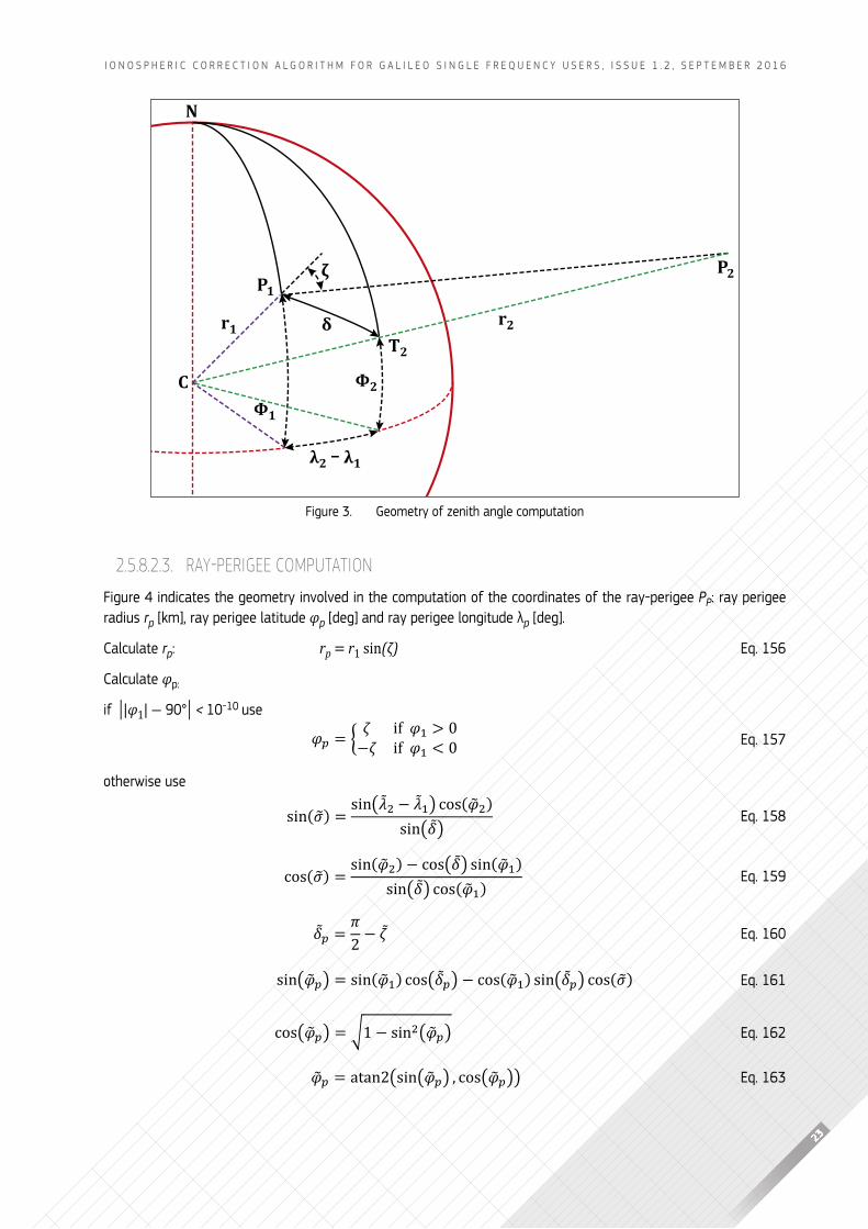
figure 3 indicates the geometry involved in the computation of the zenith angle ζ at P1. calculate:

δ being the earth angle on the great circle connecting the receiver (P1) and the satellite (P2). the symbol atan2(y,x) indicates the function that computes the arctangent of y/x with a range of (-π,π).

eq. 144

eq. 145

eq. 146

eq. 147

eq. 148

eq. 149

|𝐺𝐺𝐺𝐺1 − 𝐺𝐺𝐺𝐺2| > 𝜀𝜀|𝐺𝐺𝐺𝐺1| eq. 150

𝑇𝑇𝑇𝑇𝑇𝑇 = (𝐺𝐺𝐺𝐺2 +𝐺𝐺𝐺𝐺2 − 𝐺𝐺𝐺𝐺1

15 ) × 10−13 eq. 151

eq. 152

N

C

P2P1

T2

r2r1

λ2 � λ1

Φ1 Φ2

δ

ζ

figure 3. geometry of zenith angle computation

cos(𝛿𝛿) = sin(�̃�𝜑1) sin(�̃�𝜑2) + cos(�̃�𝜑1) cos(�̃�𝜑2) cos(�̃�𝜆2 − �̃�𝜆1) eq. 153

sin(𝛿𝛿) = √1 − cos2(𝛿𝛿) eq. 154

𝜁𝜁 = atan2 (sin(𝛿𝛿) , cos(𝛿𝛿) − 𝑟𝑟1𝑟𝑟2) eq. 155

∆𝑛𝑛=ℎ2 − ℎ1

𝑛𝑛

𝑔𝑔 = 0.5773502691896 ∙ ∆𝑛𝑛

𝑦𝑦 = 𝑔𝑔1 +∆𝑛𝑛 − 𝑔𝑔2

𝐺𝐺𝐺𝐺2 =∆𝑛𝑛2 ∙ ∑[𝐺𝐺(𝑦𝑦 + 𝑖𝑖∆𝑛𝑛) + 𝐺𝐺(𝑦𝑦 + 𝑖𝑖∆𝑛𝑛 + 𝑔𝑔)]

𝑛𝑛−1

𝑖𝑖=0

23





repeating the steps above it is now possible to compare the two values obtained to see if the target integration accuracy ε is achieved:

if

then continue increasing the number of points, redefine GN1 and repeat again.


2.5.8.2. slaNT Tec calculaTiONto compute the electron density at a point P along the slant ray-path defined by the points P1 and P2 the following specific geometrical configuration is considered.

2.5.8.2.1. gEOMETRICAL CONFIgURATION

to simplify the formulation we assume that if α is an angle in [deg], ᾶ is the same angle in [rad]:

ᾶ = α • DR

2.5.8.2.2. ZENITh ANgLE COMpUTATION

figure 3 indicates the geometry involved in the computation of the zenith angle ζ at P1. calculate:

δ being the earth angle on the great circle connecting the receiver (P1) and the satellite (P2). the symbol atan2(y,x) indicates the function that computes the arctangent of y/x with a range of (-π,π).

eq. 144

eq. 145

eq. 146

eq. 147

eq. 148

eq. 149



15 ) × 10−13 eq. 151

eq. 152

N

C

P2P1

T2

r2r1

λ2 � λ1

Φ1 Φ2

δ

ζ

figure 3. geometry of zenith angle computation

cos(𝛿𝛿) = sin(�̃�𝜑1) sin(�̃�𝜑2) + cos(�̃�𝜑1) cos(�̃�𝜑2) cos(�̃�𝜆2 − �̃�𝜆1) eq. 153

sin(𝛿𝛿) = √1 − cos2(𝛿𝛿) eq. 154

𝜁𝜁 = atan2 (sin(𝛿𝛿) , cos(𝛿𝛿) − 𝑟𝑟1𝑟𝑟2) eq. 155

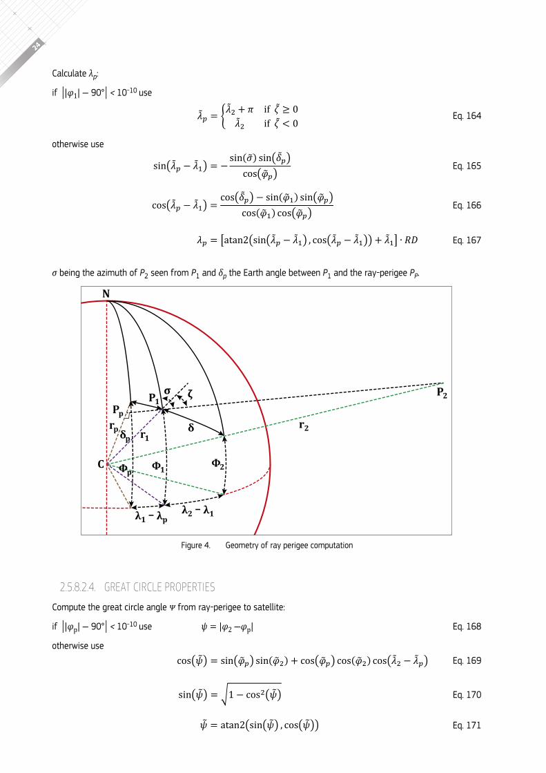
2.5.8.2.3. ray-periGee computation

figure 4 indicates the geometry involved in the computation of the coordinates of the ray-perigee PP: ray perigee radius rp [km], ray perigee latitude φp [deg] and ray perigee longitude λp [deg].

calculate rp: rp = r1 sin(ζ)

calculate φp:

if │|φ1| ― 90°│ < 10-10 use

otherwise use

eq. 156

𝜑𝜑𝑝𝑝 = { 𝜁𝜁 if 𝜑𝜑1 > 0−𝜁𝜁 if 𝜑𝜑1 < 0 eq. 157

sin(�̃�𝜎) = sin(�̃�𝜆2 − �̃�𝜆1) cos(�̃�𝜑2)sin(𝛿𝛿)

eq. 158

cos(�̃�𝜎) = sin(�̃�𝜑2) − cos(𝛿𝛿) sin(�̃�𝜑1)sin(𝛿𝛿) cos(�̃�𝜑1)

eq. 159

𝛿𝛿𝑝𝑝 =𝜋𝜋2 − 𝜁𝜁 eq. 160

sin(�̃�𝜑𝑝𝑝) = sin(�̃�𝜑1) cos(𝛿𝛿𝑝𝑝) − cos(�̃�𝜑1) sin(𝛿𝛿𝑝𝑝) cos(�̃�𝜎) eq. 161

cos(�̃�𝜑𝑝𝑝) = √1 − sin2(�̃�𝜑𝑝𝑝) eq. 162

�̃�𝜑𝑝𝑝 = atan2(sin(�̃�𝜑𝑝𝑝) , cos(�̃�𝜑𝑝𝑝)) eq. 163

24

calculate λp:

if │|φ1| ― 90°│ < 10-10 use

otherwise use

σ being the azimuth of P2 seen from P1 and δp the earth angle between P1 and the ray-perigee PP.

2.5.8.2.4. gREAT CIRCLE pROpERTIES

compute the great circle angle � from ray-perigee to satellite:

if │|φp| ― 90°│ < 10-10 use ψ = |φ2 ―φp|

otherwise use

�̃�𝜆𝑝𝑝 = {�̃�𝜆2 + 𝜋𝜋 if 𝜁𝜁 ≥ 0�̃�𝜆2 if 𝜁𝜁 < 0 eq. 164

sin��̃�𝜆𝑝𝑝 − �̃�𝜆1� = −sin(𝜎𝜎�) sin�𝛿𝛿𝑝𝑝�

cos�𝜑𝜑�𝑝𝑝� eq. 165

cos��̃�𝜆𝑝𝑝 − �̃�𝜆1� =cos�𝛿𝛿𝑝𝑝� − sin(𝜑𝜑�1) sin�𝜑𝜑�𝑝𝑝�

cos(𝜑𝜑�1) cos�𝜑𝜑�𝑝𝑝� eq. 166

𝜆𝜆𝑝𝑝 = �atan2�sin��̃�𝜆𝑝𝑝 − �̃�𝜆1� , cos��̃�𝜆𝑝𝑝 − �̃�𝜆1�� + �̃�𝜆1� ∙ 𝑅𝑅𝑅𝑅 eq. 167

N

C

P2P1Pp

r2r1rp

λ2 � λ1 λ1 � λp

Φ1 Φp Φ2

δ δp

ζ σ

figure 4. geometry of ray perigee computation

eq. 168

cos(�̃�𝜓) = sin(�̃�𝜑𝑝𝑝) sin(�̃�𝜑2) + cos(�̃�𝜑𝑝𝑝) cos(�̃�𝜑2) cos(�̃�𝜆2 − �̃�𝜆𝑝𝑝) eq. 169

sin(�̃�𝜓) = √1 − cos2(�̃�𝜓) eq. 170

�̃�𝜓 = atan2(sin(�̃�𝜓) , cos(�̃�𝜓)) eq. 171

25


compute sine and cosine of azimuth σ of satellite as seen from ray-perigee Pp:

if │|φp| ― 90°│ < 10-10 use sin(σ͂ p) = 0

otherwise use

2.5.8.2.5. INTEgRATION ENDpOINTS:

Indicating with s1 and s2 the distances of P1 and P2 respectively from the ray perigee compute:

2.5.8.2.6. COORDINATES ALONg ThE INTEgRATION pATh: c(hs, φs, λs)

with s [km] being the distance of a point P from the ray perigee PP, (rp, φp, λp) the ray perigee coordinates and sin σp, cos σp the sine and cosine of the azimuth of the satellite as seen from the ray-perigee, the coordinates of the point P are calculated by the function c as follows.

Inputs: Distance s [km], ray perigee coordinates (rp, φp, λp), sine and cosine of azimuth of satellite as seen from ray-perigee sin(σ͂ p), cos(σ͂ p)

outputs: coordinates of point P: hs [km], φs [deg], λs [deg]

to compute the geocentric coordinates of any point P (having distance s from the ray perigee PP) along the integration path, the following formulae have to be applied:

calculate hs:

where RE is the earth mean radius.

calculate the great circle parameters:

eq. 172

cos(�̃�𝜎𝑝𝑝) = {−1 if 𝜑𝜑𝑝𝑝 > 01 if 𝜑𝜑𝑝𝑝 < 0 eq. 173

sin�𝜎𝜎�𝑝𝑝� =cos(𝜑𝜑�2) sin��̃�𝜆2 − �̃�𝜆𝑝𝑝�

sin�𝜓𝜓�� eq. 174

cos�𝜎𝜎�𝑝𝑝� =sin(𝜑𝜑�2) − sin�𝜑𝜑�𝑝𝑝� cos�𝜓𝜓��

cos�𝜑𝜑�𝑝𝑝� sin�𝜓𝜓�� eq. 175

𝑠𝑠1 = √𝑟𝑟12 − 𝑟𝑟𝑝𝑝2 eq. 176

𝑠𝑠2 = √𝑟𝑟22 − 𝑟𝑟𝑝𝑝2 eq. 177

ℎ𝑠𝑠 = √𝑠𝑠2 + 𝑟𝑟𝑝𝑝2 − 𝑅𝑅𝐸𝐸 eq. 178

tan 𝛿𝛿𝑠𝑠 =𝑠𝑠𝑟𝑟𝑝𝑝

eq. 179

cos(𝛿𝛿𝑠𝑠) =1

√1 + tan2(𝛿𝛿𝑠𝑠)

eq. 180

sin(𝛿𝛿𝑠𝑠) = tan(𝛿𝛿𝑠𝑠) cos(𝛿𝛿𝑠𝑠) eq. 181

26

calculate φs:

calculate λs:

2.5.8.2.7. SLANT TEC NUMERICAL INTEgRATION

To compute slant TEc along a ray-path defined by its perigee coordinates, direction and end-point, a numerical integration algorithm is used. In NeQuick 1, a gauss integration is used and is described as follows.

Inputs: h1, height of point P1 [km]

φ1, latitude of point P 1 [deg]

λ1, longitude of point P1 [deg]

h2, height of point P2 [km]

φ2, latitude of point P2 [deg]

λ2, longitude of point P2 [deg]

Az coefficients: a0, a1, a2

month mth

UT [hours]

output: slant tec [tecu]

one possible numerical algorithm for slant tec calculation is the following.

In the case of integration from ground to satellite (h1<1000 km and h2>2000 km) it is convenient to divide the integration path in three parts defining intermediate points sa, sb:

we have that (RE + 1000)2 = 54334589.44 and (RE + 2000)2 = 70076989.44.

the slant tec becomes therefore:

sin(�̃�𝜑𝑠𝑠) = sin(�̃�𝜑𝑝𝑝) cos(𝛿𝛿𝑠𝑠) + cos(�̃�𝜑𝑝𝑝) sin(𝛿𝛿𝑠𝑠) cos(�̃�𝜎𝑝𝑝) eq. 182

cos(�̃�𝜑𝑠𝑠) = √1 − sin2(�̃�𝜑𝑠𝑠) eq. 183

eq. 184 atan2(sin(�̃�𝜑𝑠𝑠) , cos(�̃�𝜑𝑠𝑠)) ∙ 𝑅𝑅𝑅𝑅 φs =

sin(�̃�𝜆𝑠𝑠 − �̃�𝜆𝑝𝑝) = sin(𝛿𝛿𝑠𝑠) sin(�̃�𝜎𝑝𝑝) cos(�̃�𝜑𝑝𝑝) eq. 185

cos(�̃�𝜆𝑠𝑠 − �̃�𝜆𝑝𝑝) = cos(𝛿𝛿𝑠𝑠) − sin(�̃�𝜑𝑝𝑝) sin(�̃�𝜑𝑠𝑠) eq. 186

𝜆𝜆𝑠𝑠 = [atan2(sin(�̃�𝜆𝑠𝑠 − �̃�𝜆𝑝𝑝) , cos(�̃�𝜆𝑠𝑠 − �̃�𝜆𝑝𝑝)) + �̃�𝜆𝑝𝑝] ∙ 𝑅𝑅𝑅𝑅 eq. 187

𝑠𝑠𝑎𝑎 = √(𝑅𝑅𝐸𝐸 + 1000)2 − 𝑟𝑟𝑝𝑝2 eq. 188

𝑠𝑠𝑏𝑏 = √(𝑅𝑅𝐸𝐸 + 2000)2 − 𝑟𝑟𝑝𝑝2 eq. 189

𝑇𝑇𝑇𝑇𝑇𝑇 = ∫ 𝑁𝑁(𝑠𝑠)d𝑠𝑠𝑠𝑠𝑎𝑎

𝑠𝑠1

+ ∫ 𝑁𝑁(𝑠𝑠)d𝑠𝑠𝑠𝑠𝑏𝑏

𝑠𝑠𝑎𝑎

+ ∫ 𝑁𝑁(𝑠𝑠)d𝑠𝑠𝑠𝑠2

𝑠𝑠𝑏𝑏

eq. 190

27


to compute each integral, the algorithm described in section 2.5.8.2.8 can be used as

where the parameter ε indicates the integration accuracy. here we assume:

ε = 0.001 for the integration between s1 and sa

ε = 0.01 for the integrations between sa and sb and between sb and s2

2.5.8.2.8. gAUSS ALgORIThM

inputs: distances from the ray perigee of the first integration endpoint: g1 [km]

distances from the ray perigee of the second integration endpoint: g2 [km]

target integration accuracy ε - relative difference between two integration steps, recommended maximum value ε = 10-3

ray-perigee parameters: rp [km], sin(φp), cos(φp),sin(σ͂ p), cos(σ͂ p), λp [deg]

Az coefficients: a0, a1, a2

month mth

ut [hours]

output: tec [tecu]

to be able to compute NeQuick electron density, in all the following computations it is necessary to calculate the coordinates of the point P along the ray-path using the algorithm illustrated in 2.5.8.2.6:

and with a0, a1, a2, mth, uT fixed during the integration, in the following a simplified notation is used:

start the calculation using 8 points: n = 8

repeat the following computations until the target integration accuracy (ε) is obtained as follows:


∫ 𝑁𝑁(𝑠𝑠)d𝑠𝑠𝑔𝑔2

𝑔𝑔1

= 𝐺𝐺𝑁𝑁(𝑔𝑔1, 𝑔𝑔2, 𝜀𝜀, 𝑟𝑟𝑝𝑝, sin(�̃�𝜑𝑝𝑝) , cos(�̃�𝜑𝑝𝑝) , sin(�̃�𝜎𝑝𝑝) , cos(�̃�𝜎𝑝𝑝) , 𝜆𝜆𝑝𝑝, 𝑎𝑎0, 𝑎𝑎1, 𝑎𝑎2,mth, UT) eq. 191

῀ ῀

(ℎ(𝑠𝑠), 𝜑𝜑(𝑠𝑠), 𝜆𝜆(𝑠𝑠)) = 𝑐𝑐(𝑠𝑠, sin(�̃�𝜑𝑝𝑝) , cos(�̃�𝜑𝑝𝑝) , sin(�̃�𝜎𝑝𝑝) , cos(�̃�𝜎𝑝𝑝) , 𝜆𝜆𝑝𝑝) eq. 192

𝑓𝑓(𝑠𝑠):= 𝑁𝑁(ℎ(𝑠𝑠), 𝜑𝜑(𝑠𝑠), 𝜆𝜆(𝑠𝑠), 𝑎𝑎0, 𝑎𝑎1, 𝑎𝑎2,mth, UT) eq. 193

eq. 194

∆𝑛𝑛=𝑔𝑔2 − 𝑔𝑔1

𝑛𝑛 eq. 195

𝑔𝑔 = 0.5773502691896 ∙ ∆𝑛𝑛 eq. 196

𝑦𝑦 = 𝑔𝑔1 +∆𝑛𝑛 − 𝑔𝑔2 eq. 197

𝐺𝐺𝐺𝐺2 =∆𝑛𝑛2 ∙ ∑[𝑓𝑓(𝑦𝑦 + 𝑖𝑖∆𝑛𝑛) + 𝑓𝑓(𝑦𝑦 + 𝑖𝑖∆𝑛𝑛 + 𝑔𝑔)]

𝑛𝑛−1

𝑖𝑖=0 eq. 198

28



repeating steps above it is now possible to compare the two values obtained to see if the target accuracy is achieved:

if

then continue increasing the number of points, redefine GN1 and repeat again the steps above.


2.5.8.3. alTerNaTive cOMPuTaTiONal efficieNT Tec iNTeGraTiON MeThODin Section F.2.6 an alternative more computationally efficient integration method for calculating TEc along rays based on kronrod G7-k15 adaptive quadrature method is presented. this method involves sampling values at 15 points and calculating the integration from them.

2.5.9 CLARIFICATION ON COORDINATES USED IN NeQuickThe moDip table grid file used by NeQuick is calculated using the iGrF model for the Earth’s magnetic field. Strictly speaking, the coordinates derived from such a model are defined as corrected Geomagnetic coordinates (cGm), as defined in annex b.

Typical geomagnetic coordinates are those derived from a dipole approximation of the Earth’s magnetic field. in this sense, parameters that depend on dipole latitude, such as the magnetic dip i or MODiP, were defined based on geomagnetic coordinates and not cgm.

thereby, when NeQuick applies equations 204 and 205 given in Annex b for i and MODiP using cgm coordinates instead of the dipole geomagnetic coordinates, those concepts should be referred as corrected magnetic Dip (i’) and corrected modified Dip latitude (MODiP’) respectively. this distinction is usually not found on NeQuick references and is given here solely for the user’s knowledge, having no impact on the performance of the model.

2.6 DIFFERENCES bETwEEN Nequick g AND Nequick 1 AND Nequick 2

This section summarises, for information, the main algorithmic differences between the NeQuick implementation within NeQuick G and the one within Itu-r NeQuick 1 and NeQuick 2.

The most important difference between NeQuick G and versions 1 and 2 is related to the driving input parameter: for NeQuick G the driving parameter is the Effective ionisation level “Az”, based on optimisation of global observations for real-time usage and broadcast in galileo navigation message through three parameters; for NeQuick 1 and 2, the input is the monthly mean or 12 – month running solar flux (intended for climatological usage).

eq. 199

eq. 200



15 ) × 10−13 eq. 202

29


2.6.1 Summary of differenceS with NeQuick 1The main differences between NeQuick G and the Itu-r NeQuick 1 are:

● the MODiP file provided with the NeQuick G (see Annex D) and the diplats file provided with the iTu-r Fortran code correspond to different generations of the international Geomagnetic reference Field (iGrF) model, with the one in NeQuick G being newer;

● the location within the algorithm of the mapping from DIplAts to MODiP has a small effect on the computed MODiP value for the location. the impact on computed stec value can reach large values (maximum of ~5 tecu but rms of ~0.15 tecu);

● the change that has the greatest impact on computed stec values is the calculation of epstein amplitudes, e and f1 layer bottom and top thickness, and peak height. this change is accurately described in [Annex A [5]]. the reason to change the calculation of peak plasma frequency for f1 layer is also introduced in [Annex A [5]];

● The change to numerical integration method affects all STEc values to some extent (below 0.1 TEcu rms). The rationale for this change is described within [Annex A [6]];

2.6.2 Summary of differenceS with NeQuick 2The main differences between NeQuick G and NeQuick 2, included in Itu-r recommendation p.681-13, are the following:

● the revision of the topside shape parameter k:

● the Itu-r version in [Annex A [3]] incorporates a MODiP file obtained with an iGrF geomagnetic field consistent with the field when the ccir files (used internally in the model in the same manner as for NeQuick 1) were generated. that means that the MODiP file is consistent with the diplats file from NeQuick 1 and it is based on Igrf from the 1970s whereas NeQuick G is based on a MODiP file from a recent iGrF generation. NeQuick 2 authors often use also MODiP files from newer iGrF generations for other applications such as data assimilation.

𝐵𝐵𝑡𝑡𝑡𝑡𝑡𝑡𝐹𝐹2 = 𝑘𝑘 ∙ 𝐵𝐵𝑏𝑏𝑡𝑡𝑡𝑡

𝐹𝐹2

𝑘𝑘 = 3.22− 0.0538 ∙ 𝑓𝑓0𝐹𝐹2 − 0.00664 ∙ ℎ𝑚𝑚𝐹𝐹2 + 0.113ℎ𝑚𝑚𝐹𝐹2𝐵𝐵𝑏𝑏𝑏𝑏𝑏𝑏𝐹𝐹2

+ 0.00257 ∙ 𝑅𝑅12

𝑘𝑘 ≥ 1

SECTION 3: ImplEmENTaTION guIdElINES FOr uSEr rECEIvErS

31


this section describes practical guidelines for the implementation of the single-frequency ionospheric model previously described within galileo user receivers.

3.1 Zero-valued coefficientS and default EFFECTIvE IONISATION LEvEL

when all the Effective ionisation level ionospheric broadcast coefficients are set to zero:

ai0 = ai1 = ai2 =0

the coefficients shall noT be used for single-frequency ionospheric correction. in those cases, a default value shall be used for correction in the receiver:

ai0 = 63.7; ai1 = ai2 =0

this default value represents the lowest solar flux value in average conditions that NeQuick is expected to operate on. In terms of the analytical expression relating 12-month running sun spot number and solar flux (see eq. 206 within section 5.2), it corresponds to a sun spot number of 0. this value is considered adequate when no other solution is available, while still being able to correct for a significant contribution of the ionospheric delay error.

3.2 applicability and coherence of bROADCAST COEFFICIENTS

In nominal conditions, a galileo user receiver decoding the galileo navigation message from N galileo satellites simultaneously, with N >1, would receive at a given epoch, the same broadcast ionospheric coefficients for all N satellites. however, when the ionospheric parameters are updated, given that the message up-link to different satellites is not necessarily synchronised due to satellite visibility to up-link stations (uls), it may happen that some satellites broadcast the recently updated coefficients while others still broadcast the previous batch of coefficients. In such situation, any given user decoding the navigation message at any given moment does not have means to identify, which coefficients are newer and which are older. also, it has no means to decide which coefficients to apply for correction of pseudo-ranges of different satellites (either each satellite applying corrections broadcast on its own navigation message or one single set of coefficients used for correcting all satellites). nevertheless, the correction capability will still be achieved on statistical sense, independently of the adopted solution.

3.3 EFFECTIvE IONISATION LEvEL bOUNDARIESDue to the fact that the Effective ionisation level is represented simply by a second-order degree polynomial as a function of MODiP, it may exceptionally happen that for some MODiP values, the Effective ionisation parameter becomes out of range. The operational range for the Effective ionisation parameter is between 0 and 400 sfu and the following condition for out of range values should be used:

given a user receiver u with MODiP = μ

and broadcast coefficients (ai0, ai1, ai2)

32

calculate Effective ionisation level:

Azu = ai0 + ai1×μ + ai2×μ2

if Azu<0 Azu = 0

if Azu>400 Azu = 400

3.4 inteGration of nequick G into hiGher LEvEL SOFTwARE

NeQuick G requires data from 13 files, as indicated in 2.5.3 and annex c. although the convenience of integrating NeQuick G as a library with clear interfaces is convenient for many reasons, the loading of those 13 files for each Slant Delay computation introduces an unnecessary burden in terms of computation time. therefore it is recommended to integrate the pre-loading of those files outside NeQuick G in the main target software at initialisation. all the rest can be separated into a library.

3.5 COMpUTATION RATE OF IONOSphERIC CORRECTIONS

the ionosphere variations in nominal conditions are fairly slow and for the majority of applications it is not required to re-compute the delay correction at high rates. for example, in most cases, for stationary receivers or pedestrian users, it may suffice to re-compute the corrections every 30 seconds.

33


1.1.1. E5 Signal1.1.1.1. Modulation Scheme

The diagram in Figure 3 provides a generic view of the E5 signal AltBOC modulation

generation.

The E5 signal components are generated according to the following: eE5a-I from the F/NAV navigation data stream D

E5a-I modulated with the unencrypted

ranging code CE5a-I eE5a-Q (pilot component) from the unencrypted ranging code C

E5

eE5b-I from the I/NAV navigation data stream DE5b-I modulated with the unencrypted

ranging code CE5b-I eE5b-Q (pilot component) from the unencrypted ranging code C

E5b-Q

-

The ionosphere is a region of weakly ionised gas in the Earth’s atmosphere lying between about 50 kilometers up to several thousand kilome-ters from Earth’s surface. Solar radiation is responsible for this ionisation producing free electrons and ions. The iono-spheric refractive index (the ratio between the speed of propagation in the media and the speed of propagation in vacuum) is related to the number of free electrons through the propagation path. For this purpose, the Total Electron Content (TEC) is

in a cross-section of 1m2, integrated along a slant (or vertical) path between two points (e.g. a satellite and a receiver); it is expressed in TEC units (TECU) where 1TECU equals 1016 electrons/m2. The

propagation in various ways such as refraction, absorption, Faraday rotation, group delay, time dispersion or scintillations, being most of them related to TEC in the propagation path.

they depend on the signal frequency.

The ionosphere is classically sub-divided in layers character-

E, F1 and F2, the latter being largely responsible for the

-tions.

N

C

P2P1Pp

r2r1rp

λ2 � λ1 λ1 � λp

Φ1 Φp Φ2

δ δp

ζ σ

AltBOCMUX

CE5a-I

DE5a-ICE5a-Q

eE5a-I

eE5a-Q

CE5b-I

sE5

DE5b-ICE5b-Q

eE5b-I

eE5b-Q

3 , = 31, , ( 1 −100

) + 32, , 100

aNNEx a: applICaBlE aNd rEFErENCE dOCumENTS

35


A.1. AppLICAbLE DOCUMENTS[1] European GNSS (Galileo) Open Service Signal In Space Interface Control Document (OS SIS

icD), Issue 1.2, european union, 2015

A.2. REFERENCE DOCUMENTS[2] Minimal Operational Performance Standards for GPS/WAAS Airborne Equipment, rtcA-Do

229 c, november. 2001.

[3] ITU-R, Ionospheric propagation data and prediction methods required for the design of satellite services and systems, rec. Itu-r p. 531-11, january 2012.

[4] ITU-R, choices if indices for long-term ionospheric predictions, rec. Itu-r p.371-8, 1999.

[5] Leitinger, r.; zhang, m.-l.; radicella, s.m., An improved bottomside for the ionospheric electron density model NeQuick, ann. Geophys., vol. 48, no. 3, p. 525-534, 2005.

[6] knezevich, m.; radicella, s.m., Development of an ionospheric NeQuick model algorithm for GNSS receivers, in naviTEc 2004, noordwijk, 2004.

[7] corrected Geomagnetic coordinates, [online], naSa vitmo models, http://omniweb.gsfc.nasa.gov/vitmo/cgmm_des.html, 12th september 2013

[8] Rawer, k., Meteorological and Astronomical influences on Radio Wave Propagation, b. landmark (ed.), chapter 11. propagation of Decameter waves (h.f. band), p. 221, Academic press new york, 1963

[9] international Geomagnetic Reference Field, [online], IAgA geomagnetic field modeling, http://www.ngdc.noaa.gov/IAgA/vmod/igrf.html, 12th september 2013

[10] klobuchar, j., An Ionospheric Time-Delay Algorithm for Single-Frequency GPS Users, Ieee transactions on Aerospace and electronic systems, Aes-23 (3), 325–331, 1987

[11] r. prieto-cerdeira, r. orus-perez, e. breeuwer, r. lucas-rodriguez, m. falcone, The European Way: Assessment of NeQuick Ionospheric Model for Galileo Single-Frequency Users, gps world, vol. 25, no. 6, pp. 53–58, 2014.

[12] mosert de gonzalez, m.; radicella, s.m., On a characteristic point at the base of F2 layer in the ionosphere, adv. Space res., vol. 10, iss. 11, 1990

[13] Di giovanni, g.; radicella, s.m., An analytical model of the electron density profile in the ionosphere, adv. Space res., vol. 10, no. 11, p. 27-30, 1990.

[14] radicella, s.m.; zhang, m.-l., The improved DGR analytical model of electron density height profile and total electron content in the ionosphere, ann. Geofis, vol. xxxviii, no. 1, p. 35-41, 1995

[15] radicella, s.m., leitinger, r., The evolution of the DGR approach to model electron density profiles, Adv. space res�, vol. 27, no. 1, p. 35-40, 2001.

[16] http://utd500.utdallas.edu/ionosphere.htm

http://omniweb.gsfc.nasa.gov/vitmo/cgmm_des.html

http://omniweb.gsfc.nasa.gov/vitmo/cgmm_des.html

http://www.ngdc.noaa.gov/IAGA/vmod/igrf.html

http://www.ngdc.noaa.gov/IAGA/vmod/igrf.html

aNNEx B: aCrONymS aNd dEFINITIONS

37


b.1. acronymSec european commission

esA european space Agency

foc full operational capability

GiovE Galileo in orbit validation Element

gnss global navigation satellite system

gsA european gnss Agency

Ictp Abdus salam International center of theoretical physics

iov in orbit validation

Igrf International geomagnetic reference field

Igs International gnss service

MODiP modified Dip latitude

nSl nottingham Scientific ltd

os open service

rms root mean square

sIsIcD signal In space Interface control Document

sfIono galileo single frequency Ionospheric Algorithm

sfu solar flux units

stec slant total electron content

tec total electron content

uere user equivalent ranging error

b.2. DEFINITIONSCCIR files: numerical grid maps which describe the regular variation of the ionosphere. they are used to derive other variables such as critical frequencies and transmission factors. In NeQuick, foF2 and M(3000)F2 are derived from R12 and the ccir files.

Corrected Geomagnetic Coordinates (CGM): coordinates relative to Earth’s magnetic field when this is not approximated from a dipole but instead calculated from a model, usually the International geomagnetic reference field (Igrf) model [Annex A [7]].

Critical frequency (fo): maximum frequency for which an electromagnetic wave is reflected at vertical incidence. It is usually referred to a particular layer, e.g., foe, foF1 and foF2. At frequencies larger than the critical frequency, the radio wave penetrates the layer. It is expressed in hz.

Effective Ionisation Level (Az): index that represents solar activity in the same fashion as F10�7. It is used to drive NeQuick model for a daily use in galileo, instead of the monthly mean original behaviour when using F10�7. It is also expressed in sfu this parameter is valid for the whole world. the Az parameter is a continuous function of the MODiP at the receiver location. Az is expressed by three coefficients:

Az = ai0 + ai1 × MODiP + ai2 × (MODiP)2

The three coefficients, ai0, ai1 and ai2 are transmitted to the users in the galileo navigation broadcast message.

Geomagnetic Coordinates: coordinates relative to Earth’s magnetic field when this is approximated by a dipole. for the dipole approximation, the centred dipole axis cuts the earth’s surface at the south and north dipole poles. the dipole axis is inclined at about 11deg to the axis of rotation [Annex A [7]]. the plane through earth’s centre perpendicular to the dipole axis is called the dipole equator. the geomagnetic coordinates or dipole coordinates (dipole latitude and dipole longitude) are reckoned relative to the dipole axis, dipole poles and dipole equator. the relation between dipole and geographic coordinates can be found in [Annex A [7]].

eq. 203

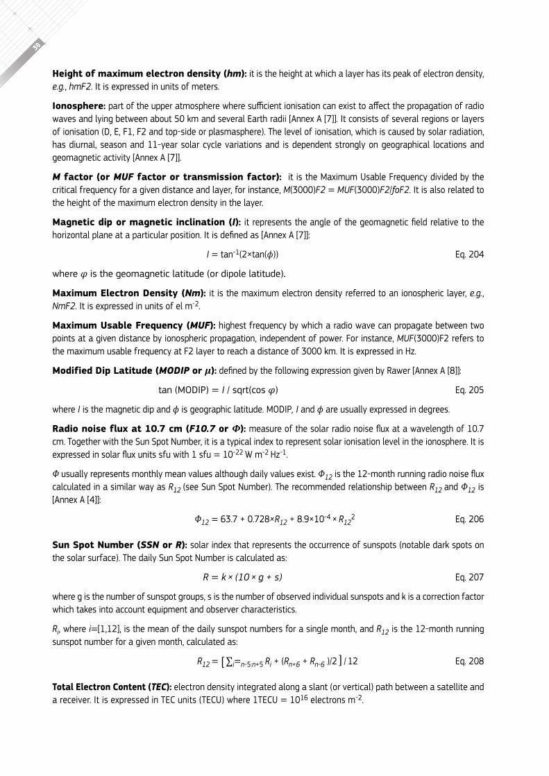
38

Height of maximum electron density (hm): it is the height at which a layer has its peak of electron density, e�g�, hmF2. It is expressed in units of meters.

Ionosphere: part of the upper atmosphere where sufficient ionisation can exist to affect the propagation of radio waves and lying between about 50 km and several earth radii [Annex A [7]]. It consists of several regions or layers of ionisation (D, e, f1, f2 and top-side or plasmasphere). the level of ionisation, which is caused by solar radiation, has diurnal, season and 11-year solar cycle variations and is dependent strongly on geographical locations and geomagnetic activity [Annex A [7]].

M factor (or MUF factor or transmission factor): it is the maximum usable frequency divided by the critical frequency for a given distance and layer, for instance, M(3000)F2 = MuF(3000)F2/foF2. It is also related to the height of the maximum electron density in the layer.

Magnetic dip or magnetic inclination (I): it represents the angle of the geomagnetic field relative to the horizontal plane at a particular position. it is defined as [annex a [7]]:

i = tan-1(2×tan(φ))

where φ is the geomagnetic latitude (or dipole latitude).

Maximum Electron Density (Nm): it is the maximum electron density referred to an ionospheric layer, e�g�, NmF2. It is expressed in units of el m-2.

Maximum Usable Frequency (MUF): highest frequency by which a radio wave can propagate between two points at a given distance by ionospheric propagation, independent of power. for instance, MuF(3000)f2 refers to the maximum usable frequency at f2 layer to reach a distance of 3000 km. It is expressed in hz.

Modified Dip Latitude (MODIP or μ): defined by the following expression given by rawer [annex a [8]]:

tan (moDIp) = i / sqrt(cos φ)

where i is the magnetic dip and φ is geographic latitude. moDIp, i and φ are usually expressed in degrees.

Radio noise flux at 10.7 cm (F10.7 or Φ): measure of the solar radio noise flux at a wavelength of 10.7 cm. together with the sun spot number, it is a typical index to represent solar ionisation level in the ionosphere. It is expressed in solar flux units sfu with 1 sfu = 10-22 w m-2 hz-1.

Φ usually represents monthly mean values although daily values exist. Φ12 is the 12-month running radio noise flux calculated in a similar way as R12 (see sun spot number). the recommended relationship between R12 and Φ12 is [Annex A [4]]:

Φ12 = 63.7 + 0.728×R12 + 8.9×10-4 × R122

Sun Spot Number (SSN or R): solar index that represents the occurrence of sunspots (notable dark spots on the solar surface). the daily sun spot number is calculated as:

R = k × (10 × g + s)

where g is the number of sunspot groups, s is the number of observed individual sunspots and k is a correction factor which takes into account equipment and observer characteristics.

Ri, where i=[1,12], is the mean of the daily sunspot numbers for a single month, and R12 is the 12-month running sunspot number for a given month, calculated as:

R12 = [ ∑i=n-5:n+5 Ri + (Rn+6 + Rn-6 )/2 ] / 12

Total Electron Content (TEC): electron density integrated along a slant (or vertical) path between a satellite and a receiver. It is expressed in tec units (tecu) where 1tecu = 1016 electrons m-2.

eq. 204

eq. 205

eq. 206

eq. 207

eq. 208

39


aNNEx C: COmplEmENTary fileS(ccirandmodip)

41


These files are only provided in the electronic version of this document, which can be found at http://www.gsc-europa.eu/system/files/galileo_documents/galileo_Ionospheric_model.pdf

This annex contains the complementary files required by NeQuick G. There are 12 ccir files and one MODiP grid file.

aNNEx d: NEquICk g pErFOrmaNCE rESulTS

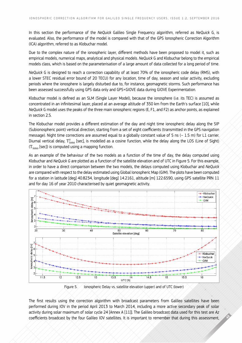
43


In this section the performance of the NeQuick galileo single frequency algorithm, referred as NeQuick g, is evaluated. Also, the performance of the model is compared with that of the gps Ionospheric correction Algorithm (IcA) algorithm, referred to as klobuchar model.

Due to the complex nature of the ionospheric layer, different methods have been proposed to model it, such as empirical models, numerical maps, analytical and physical models. NeQuick g and klobuchar belong to the empirical models class, which is based on the parameterisation of a large amount of data collected for a long period of time.

NeQuick G is designed to reach a correction capability of at least 70% of the ionospheric code delay (rmS), with a lower stec residual error bound of 20 tecu) for any location, time of day, season and solar activity, excluding periods where the ionosphere is largely disturbed due to, for instance, geomagnetic storms. such performance has been assessed successfully using GpS data only and GpS+GiovE data during GiovE Experimentation.

Klobuchar model is defined as an Slm (Single layer model), because the ionosphere (i.e. its TEc) is assumed as concentrated in an infinitesimal layer, placed at an average altitude of 350 km from the Earth's surface [10], while NeQuick g model uses the peaks of the three main ionospheric regions (e, f1, and f2) as anchor points, as explained in section 2.5.

The Klobuchar model provides a different estimation of the day and night time ionospheric delay along the Sip (Subionospheric point) vertical direction, starting from a set of eight coefficients (transmitted in the GpS navigation message). night time corrections are assumed equal to a globally constant value of 5 ns (~ 1.5 m) for l1 carrier. Diurnal vertical delay, T viono [sec], is modelled as a cosine function, while the delay along the los (line of sight) (T iono [sec]) is computed using a mapping function.

As an example of the behaviour of the two models as a function of the time of day, the delay computed using klobuchar and NeQuick G are plotted as a function of the satellite elevation and of utc in figure 5. for this example, in order to have a direct comparison between the two models, the delays computed using klobuchar and NeQuick are compared with respect to the delay estimated using global Ionospheric map (gIm). the plots have been computed for a station in latitude [deg] 40.8234, longitude [deg] 14.2161, altitude [m] 122.6590, using gps satellite prn 11 and for day 16 of year 2010 characterised by quiet geomagnetic activity.

The first results using the correction algorithm with broadcast parameters from Galileo satellites have been performed during iov in the period april 2013 to march 2014, including a more active secondary peak of solar activity during solar maximum of solar cycle 24 [Annex A [11]]. the galileo broadcast data used for this test are Az coefficients broadcast by the four Galileo iov satellites. it is important to remember that during this assessment,

figure 5. Ionospheric Delay vs. satellite elevation (upper) and of utc (lower)

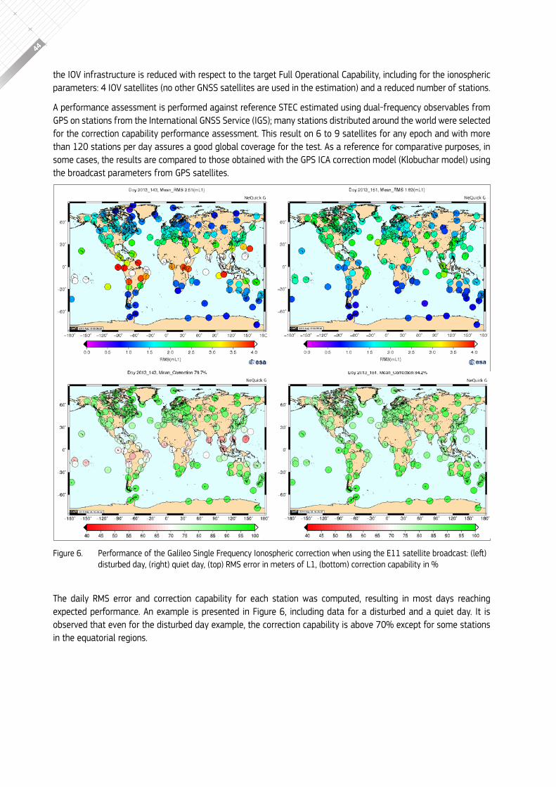
44

the iov infrastructure is reduced with respect to the target Full operational capability, including for the ionospheric parameters: 4 iov satellites (no other GnSS satellites are used in the estimation) and a reduced number of stations.

A performance assessment is performed against reference stec estimated using dual-frequency observables from gps on stations from the International gnss service (Igs); many stations distributed around the world were selected for the correction capability performance assessment. this result on 6 to 9 satellites for any epoch and with more than 120 stations per day assures a good global coverage for the test. As a reference for comparative purposes, in some cases, the results are compared to those obtained with the gps IcA correction model (klobuchar model) using the broadcast parameters from gps satellites.

the daily rms error and correction capability for each station was computed, resulting in most days reaching expected performance. An example is presented in figure 6, including data for a disturbed and a quiet day. It is observed that even for the disturbed day example, the correction capability is above 70% except for some stations in the equatorial regions.

figure 6. performance of the Galileo Single Frequency ionospheric correction when using the E11 satellite broadcast: (left) disturbed day, (right) quiet day, (top) rmS error in meters of l1, (bottom) correction capability in %

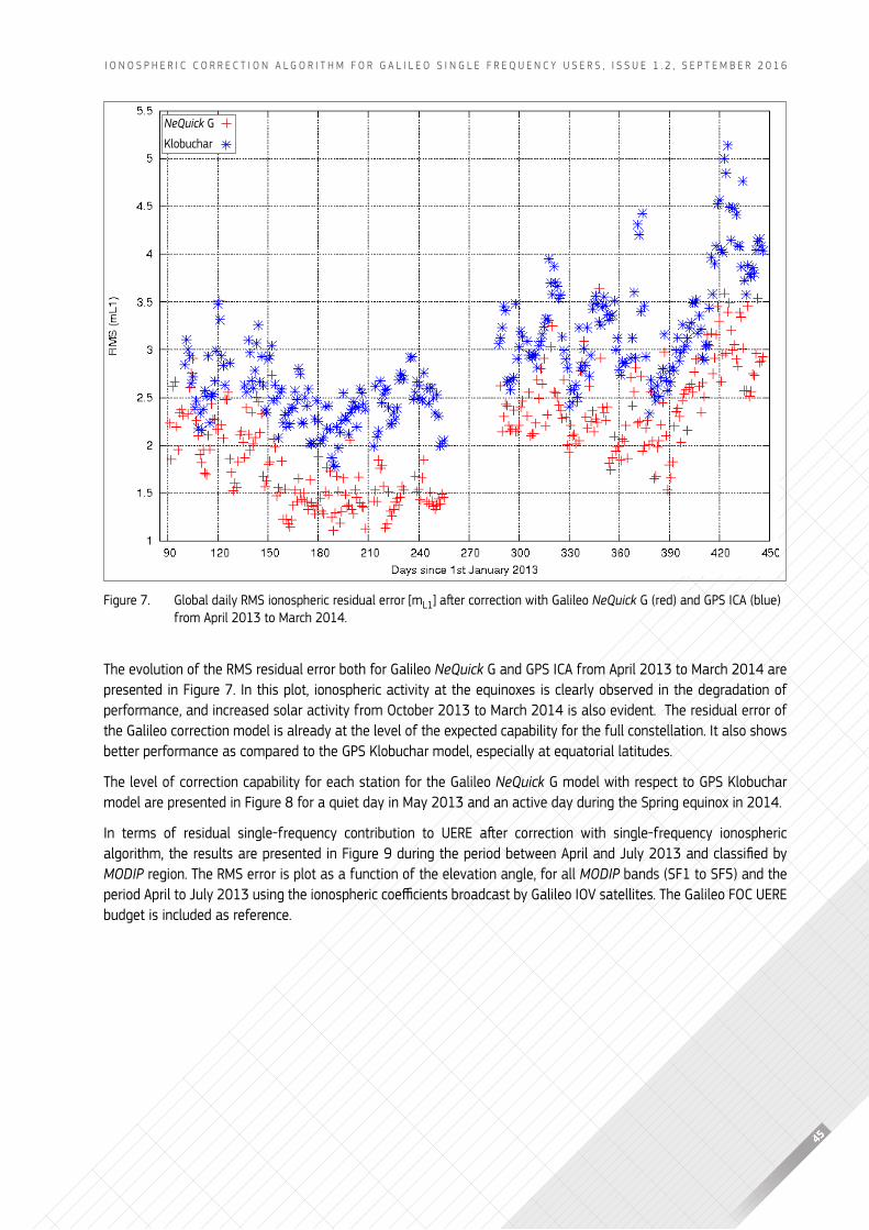
45


the evolution of the rms residual error both for galileo NeQuick g and gps IcA from April 2013 to march 2014 are presented in figure 7. In this plot, ionospheric activity at the equinoxes is clearly observed in the degradation of performance, and increased solar activity from october 2013 to march 2014 is also evident. the residual error of the galileo correction model is already at the level of the expected capability for the full constellation. It also shows better performance as compared to the gps klobuchar model, especially at equatorial latitudes.

the level of correction capability for each station for the galileo NeQuick g model with respect to gps klobuchar model are presented in figure 8 for a quiet day in may 2013 and an active day during the spring equinox in 2014.

in terms of residual single-frequency contribution to uErE after correction with single-frequency ionospheric algorithm, the results are presented in Figure 9 during the period between april and July 2013 and classified by MODiP region. the rms error is plot as a function of the elevation angle, for all MODiP bands (sf1 to sf5) and the period april to July 2013 using the ionospheric coefficients broadcast by Galileo iov satellites. The Galileo Foc uErE budget is included as reference.

NeQuick g

klobuchar

figure 7. global daily rms ionospheric residual error [ml1] after correction with Galileo NeQuick g (red) and gps IcA (blue) from April 2013 to march 2014.

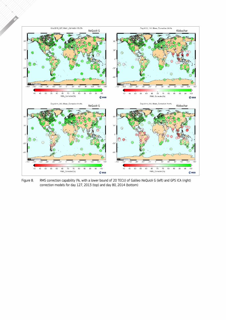
46

figure 8. rmS correction capability (%, with a lower bound of 20 TEcu) of Galileo NeQuick G (left) and GpS ica (right) correction models for day 127, 2013 (top) and day 80, 2014 (bottom)

NeQuick g

NeQuick g

klobuchar

klobuchar

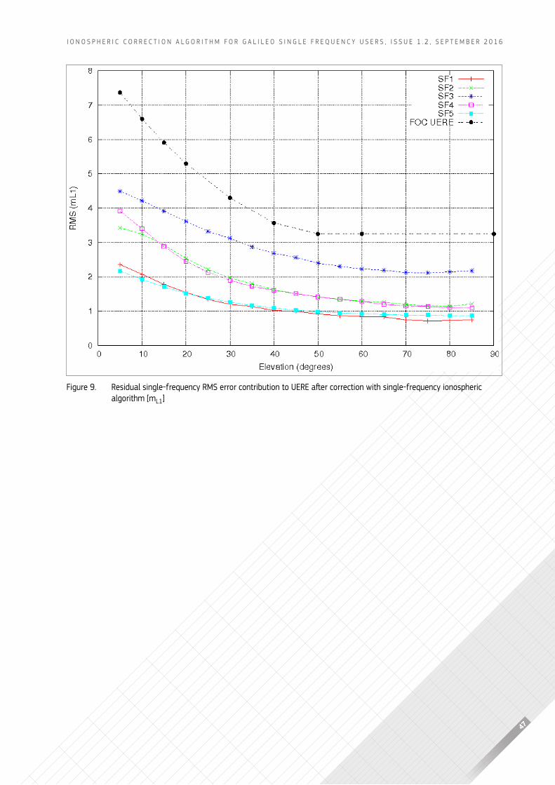
47


figure 9. residual single-frequency rmS error contribution to uErE after correction with single-frequency ionospheric algorithm [ml1]

aNNEx E: INpuT/OuTpuT vErIFICaTION daTa

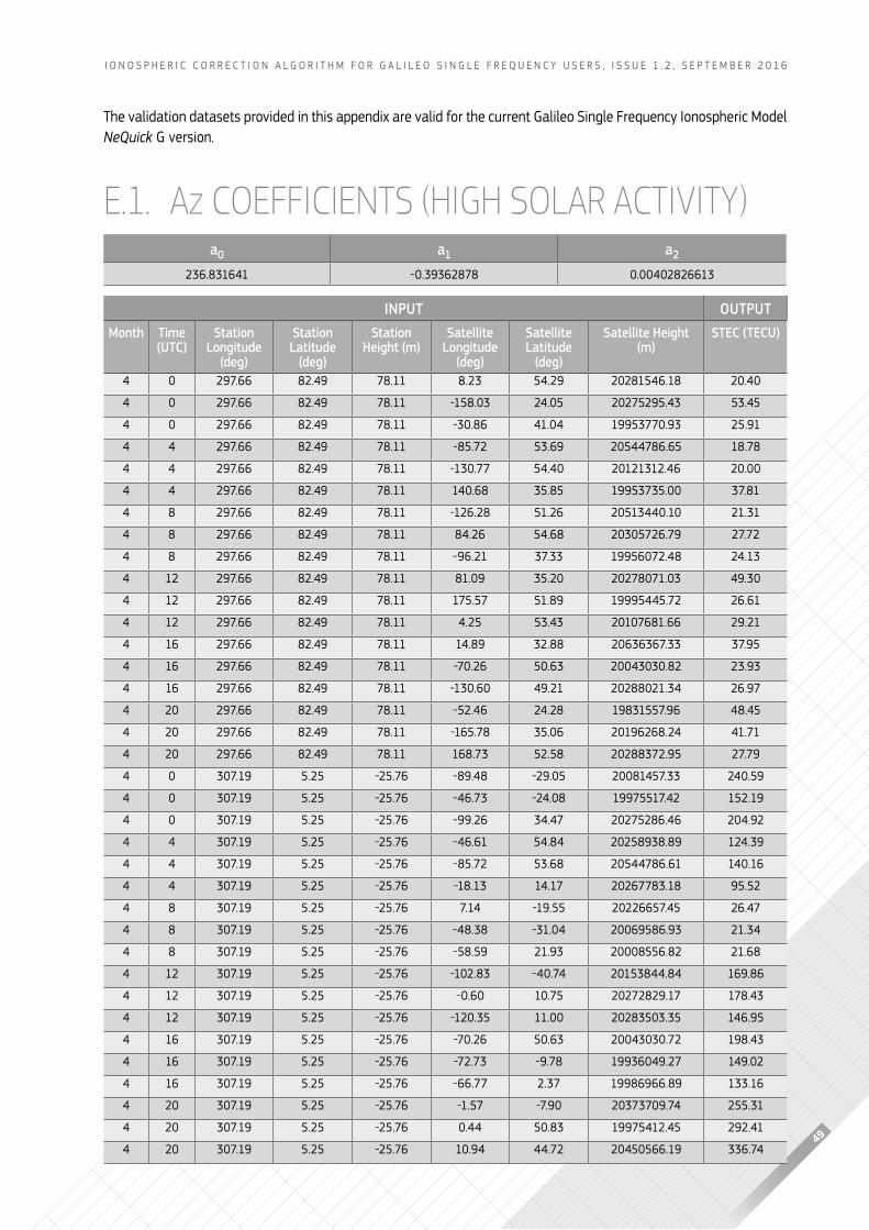
49


the validation datasets provided in this appendix are valid for the current galileo single frequency Ionospheric model NeQuick g version.

E.1. Az coefficientS (hiGh Solar activity)

INPUt OUtPUtmonth time

(UtC)Station

longitude (deg)

Station latitude

(deg)

Station height (m)

Satellite longitude

(deg)

Satellite latitude

(deg)

Satellite height (m)

StEC (tECU)

4 0 297.66 82.49 78.11 8.23 54.29 20281546.18 20.40

4 0 297.66 82.49 78.11 -158.03 24.05 20275295.43 53.45

4 0 297.66 82.49 78.11 -30.86 41.04 19953770.93 25.91

4 4 297.66 82.49 78.11 -85.72 53.69 20544786.65 18.78

4 4 297.66 82.49 78.11 -130.77 54.40 20121312.46 20.00

4 4 297.66 82.49 78.11 140.68 35.85 19953735.00 37.81

4 8 297.66 82.49 78.11 -126.28 51.26 20513440.10 21.31

4 8 297.66 82.49 78.11 84.26 54.68 20305726.79 27.72

4 8 297.66 82.49 78.11 -96.21 37.33 19956072.48 24.13

4 12 297.66 82.49 78.11 81.09 35.20 20278071.03 49.30

4 12 297.66 82.49 78.11 175.57 51.89 19995445.72 26.61

4 12 297.66 82.49 78.11 4.25 53.43 20107681.66 29.21

4 16 297.66 82.49 78.11 14.89 32.88 20636367.33 37.95

4 16 297.66 82.49 78.11 -70.26 50.63 20043030.82 23.93

4 16 297.66 82.49 78.11 -130.60 49.21 20288021.34 26.97

4 20 297.66 82.49 78.11 -52.46 24.28 19831557.96 48.45

4 20 297.66 82.49 78.11 -165.78 35.06 20196268.24 41.71

4 20 297.66 82.49 78.11 168.73 52.58 20288372.95 27.79

4 0 307.19 5.25 -25.76 -89.48 -29.05 20081457.33 240.59

4 0 307.19 5.25 -25.76 -46.73 -24.08 19975517.42 152.19

4 0 307.19 5.25 -25.76 -99.26 34.47 20275286.46 204.92

4 4 307.19 5.25 -25.76 -46.61 54.84 20258938.89 124.39

4 4 307.19 5.25 -25.76 -85.72 53.68 20544786.61 140.16

4 4 307.19 5.25 -25.76 -18.13 14.17 20267783.18 95.52

4 8 307.19 5.25 -25.76 7.14 -19.55 20226657.45 26.47

4 8 307.19 5.25 -25.76 -48.38 -31.04 20069586.93 21.34

4 8 307.19 5.25 -25.76 -58.59 21.93 20008556.82 21.68

4 12 307.19 5.25 -25.76 -102.83 -40.74 20153844.84 169.86

4 12 307.19 5.25 -25.76 -0.60 10.75 20272829.17 178.43

4 12 307.19 5.25 -25.76 -120.35 11.00 20283503.35 146.95

4 16 307.19 5.25 -25.76 -70.26 50.63 20043030.72 198.43

4 16 307.19 5.25 -25.76 -72.73 -9.78 19936049.27 149.02

4 16 307.19 5.25 -25.76 -66.77 2.37 19986966.89 133.16

4 20 307.19 5.25 -25.76 -1.57 -7.90 20373709.74 255.31

4 20 307.19 5.25 -25.76 0.44 50.83 19975412.45 292.41

4 20 307.19 5.25 -25.76 10.94 44.72 20450566.19 336.74

a0 a1 a2

236.831641 -0.39362878 0.00402826613

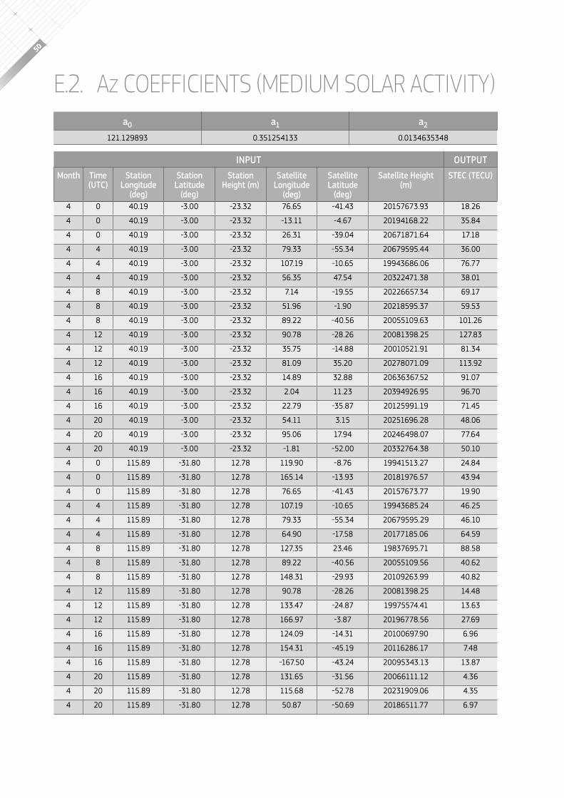
50

E.2. Az coefficientS (medium Solar activity)


(UtC)Station

longitude (deg)

Station latitude

(deg)

Station height (m)

Satellite longitude

(deg)

Satellite latitude

(deg)


StEC (tECU)

4 0 40.19 -3.00 -23.32 76.65 -41.43 20157673.93 18.26

4 0 40.19 -3.00 -23.32 -13.11 -4.67 20194168.22 35.84

4 0 40.19 -3.00 -23.32 26.31 -39.04 20671871.64 17.18

4 4 40.19 -3.00 -23.32 79.33 -55.34 20679595.44 36.00

4 4 40.19 -3.00 -23.32 107.19 -10.65 19943686.06 76.77

4 4 40.19 -3.00 -23.32 56.35 47.54 20322471.38 38.01

4 8 40.19 -3.00 -23.32 7.14 -19.55 20226657.34 69.17

4 8 40.19 -3.00 -23.32 51.96 -1.90 20218595.37 59.53

4 8 40.19 -3.00 -23.32 89.22 -40.56 20055109.63 101.26

4 12 40.19 -3.00 -23.32 90.78 -28.26 20081398.25 127.83

4 12 40.19 -3.00 -23.32 35.75 -14.88 20010521.91 81.34

4 12 40.19 -3.00 -23.32 81.09 35.20 20278071.09 113.92

4 16 40.19 -3.00 -23.32 14.89 32.88 20636367.52 91.07

4 16 40.19 -3.00 -23.32 2.04 11.23 20394926.95 96.70

4 16 40.19 -3.00 -23.32 22.79 -35.87 20125991.19 71.45

4 20 40.19 -3.00 -23.32 54.11 3.15 20251696.28 48.06

4 20 40.19 -3.00 -23.32 95.06 17.94 20246498.07 77.64

4 20 40.19 -3.00 -23.32 -1.81 -52.00 20332764.38 50.10

4 0 115.89 -31.80 12.78 119.90 -8.76 19941513.27 24.84

4 0 115.89 -31.80 12.78 165.14 -13.93 20181976.57 43.94

4 0 115.89 -31.80 12.78 76.65 -41.43 20157673.77 19.90

4 4 115.89 -31.80 12.78 107.19 -10.65 19943685.24 46.25

4 4 115.89 -31.80 12.78 79.33 -55.34 20679595.29 46.10

4 4 115.89 -31.80 12.78 64.90 -17.58 20177185.06 64.59

4 8 115.89 -31.80 12.78 127.35 23.46 19837695.71 88.58

4 8 115.89 -31.80 12.78 89.22 -40.56 20055109.56 40.62

4 8 115.89 -31.80 12.78 148.31 -29.93 20109263.99 40.82

4 12 115.89 -31.80 12.78 90.78 -28.26 20081398.25 14.48

4 12 115.89 -31.80 12.78 133.47 -24.87 19975574.41 13.63

4 12 115.89 -31.80 12.78 166.97 -3.87 20196778.56 27.69

4 16 115.89 -31.80 12.78 124.09 -14.31 20100697.90 6.96

4 16 115.89 -31.80 12.78 154.31 -45.19 20116286.17 7.48

4 16 115.89 -31.80 12.78 -167.50 -43.24 20095343.13 13.87

4 20 115.89 -31.80 12.78 131.65 -31.56 20066111.12 4.36

4 20 115.89 -31.80 12.78 115.68 -52.78 20231909.06 4.35

4 20 115.89 -31.80 12.78 50.87 -50.69 20186511.77 6.97

a0 a1 a2

121.129893 0.351254133 0.0134635348

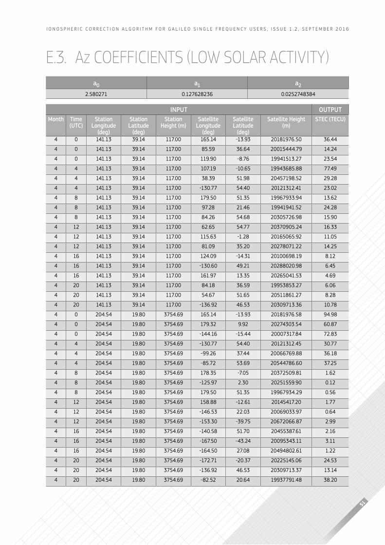
51


E.3. Az coefficientS (low Solar activity)a0 a1 a2

2.580271 0.127628236 0.0252748384


(UtC)Station

longitude (deg)

Station latitude

(deg)

Station height (m)

Satellite longitude

(deg)

Satellite latitude

(deg)


StEC (tECU)

4 0 141.13 39.14 117.00 165.14 -13.93 20181976.50 36.44

4 0 141.13 39.14 117.00 85.59 36.64 20015444.79 14.24

4 0 141.13 39.14 117.00 119.90 -8.76 19941513.27 23.54

4 4 141.13 39.14 117.00 107.19 -10.65 19943685.88 77.49

4 4 141.13 39.14 117.00 38.39 51.98 20457198.52 29.28

4 4 141.13 39.14 117.00 -130.77 54.40 20121312.41 23.02

4 8 141.13 39.14 117.00 179.50 51.35 19967933.94 13.62

4 8 141.13 39.14 117.00 97.28 21.46 19941941.52 24.28

4 8 141.13 39.14 117.00 84.26 54.68 20305726.98 15.90

4 12 141.13 39.14 117.00 62.65 54.77 20370905.24 16.33

4 12 141.13 39.14 117.00 115.63 -1.28 20165065.92 11.05

4 12 141.13 39.14 117.00 81.09 35.20 20278071.22 14.25

4 16 141.13 39.14 117.00 124.09 -14.31 20100698.19 8.12

4 16 141.13 39.14 117.00 -130.60 49.21 20288020.98 6.45

4 16 141.13 39.14 117.00 161.97 13.35 20265041.53 4.69

4 20 141.13 39.14 117.00 84.18 36.59 19953853.27 6.06

4 20 141.13 39.14 117.00 54.67 51.65 20511861.27 8.28

4 20 141.13 39.14 117.00 -136.92 46.53 20309713.36 10.78

4 0 204.54 19.80 3754.69 165.14 -13.93 20181976.58 94.98

4 0 204.54 19.80 3754.69 179.32 9.92 20274303.54 60.87

4 0 204.54 19.80 3754.69 -144.16 -15.44 20007317.84 72.83

4 4 204.54 19.80 3754.69 -130.77 54.40 20121312.45 30.77

4 4 204.54 19.80 3754.69 -99.26 37.44 20066769.88 36.18

4 4 204.54 19.80 3754.69 -85.72 53.69 20544786.60 37.25

4 8 204.54 19.80 3754.69 178.35 -7.05 20372509.81 1.62

4 8 204.54 19.80 3754.69 -125.97 2.30 20251559.90 0.12

4 8 204.54 19.80 3754.69 179.50 51.35 19967934.29 0.56

4 12 204.54 19.80 3754.69 158.88 -12.61 20145417.20 1.77

4 12 204.54 19.80 3754.69 -146.53 22.03 20069033.97 0.64

4 12 204.54 19.80 3754.69 -153.30 -39.75 20672066.87 2.99

4 16 204.54 19.80 3754.69 -140.58 51.70 20455387.61 2.16

4 16 204.54 19.80 3754.69 -167.50 -43.24 20095343.11 3.11

4 16 204.54 19.80 3754.69 -164.50 27.08 20494802.61 1.22

4 20 204.54 19.80 3754.69 -172.71 -20.37 20225145.06 24.53

4 20 204.54 19.80 3754.69 -136.92 46.53 20309713.37 13.14

4 20 204.54 19.80 3754.69 -82.52 20.64 19937791.48 38.20

aNNEx F: Nequick g dETaIlEd prOCESSINg mOdEl

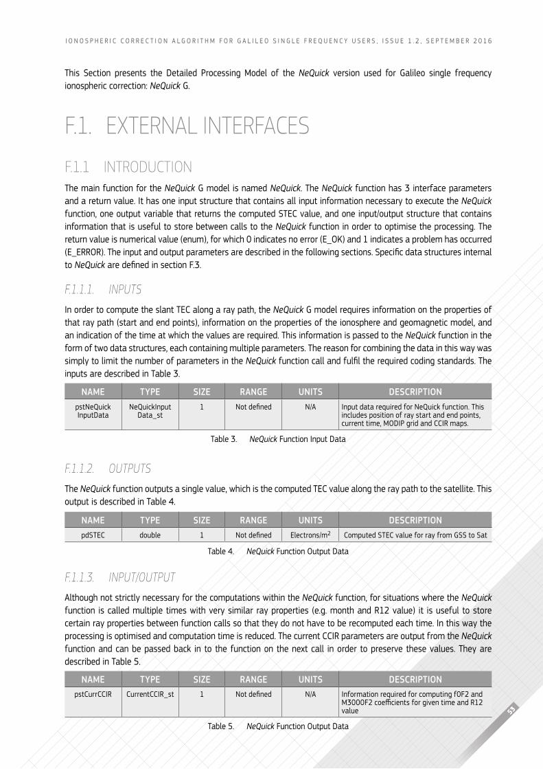
53


this section presents the Detailed processing model of the NeQuick version used for galileo single frequency ionospheric correction: NeQuick g.

F.1. EXTERNAL INTERFACES

F.1.1 INTRODUCTIONthe main function for the NeQuick g model is named NeQuick. the NeQuick function has 3 interface parameters and a return value. It has one input structure that contains all input information necessary to execute the NeQuick function, one output variable that returns the computed stec value, and one input/output structure that contains information that is useful to store between calls to the NeQuick function in order to optimise the processing. the return value is numerical value (enum), for which 0 indicates no error (e_ok) and 1 indicates a problem has occurred (E_Error). The input and output parameters are described in the following sections. Specific data structures internal to NeQuick are defined in section F.3.

f.1.1.1. iNPuTsIn order to compute the slant tec along a ray path, the NeQuick g model requires information on the properties of that ray path (start and end points), information on the properties of the ionosphere and geomagnetic model, and an indication of the time at which the values are required. this information is passed to the NeQuick function in the form of two data structures, each containing multiple parameters. the reason for combining the data in this way was simply to limit the number of parameters in the NeQuick function call and fulfil the required coding standards. The inputs are described in table 3.

f.1.1.2. OuTPuTsthe NeQuick function outputs a single value, which is the computed tec value along the ray path to the satellite. this output is described in table 4.

f.1.1.3. iNPuT/OuTPuT Although not strictly necessary for the computations within the NeQuick function, for situations where the NeQuick function is called multiple times with very similar ray properties (e.g. month and r12 value) it is useful to store certain ray properties between function calls so that they do not have to be recomputed each time. In this way the processing is optimised and computation time is reduced. the current ccIr parameters are output from the NeQuick function and can be passed back in to the function on the next call in order to preserve these values. they are described in table 5.

NAmE tyPE SIzE RANGE UNItS DESCRIPtIONpstnequick InputData

nequickInput Data_st

1 not defined n/A Input data required for nequick function. this includes position of ray start and end points, current time, moDIp grid and ccIr maps.

table 3. NeQuick function Input Data

NAmE tyPE SIzE RANGE UNItS DESCRIPtIONpdstec double 1 not defined electrons/m2 computed stec value for ray from gss to sat

table 4. NeQuick function output Data

NAmE tyPE SIzE RANGE UNItS DESCRIPtIONpstcurrccIr currentccIr_st 1 not defined n/A Information required for computing f0f2 and

m3000F2 coefficients for given time and r12 value


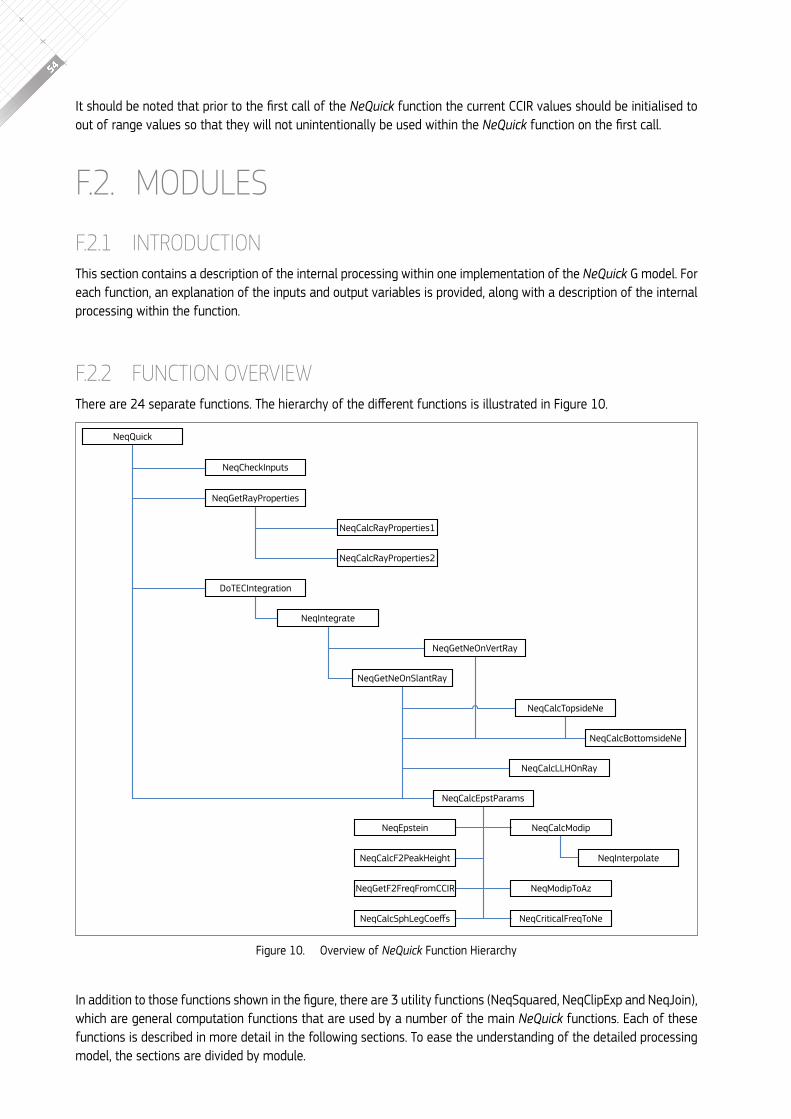
54

it should be noted that prior to the first call of the NeQuick function the current ccIr values should be initialised to out of range values so that they will not unintentionally be used within the NeQuick function on the first call.

F.2. MODULES

F.2.1 INTRODUCTIONthis section contains a description of the internal processing within one implementation of the NeQuick g model. for each function, an explanation of the inputs and output variables is provided, along with a description of the internal processing within the function.

F.2.2 FUNCTION OvERvIEwThere are 24 separate functions. The hierarchy of the different functions is illustrated in Figure 10.

in addition to those functions shown in the figure, there are 3 utility functions (neqSquared, neqclipExp and neqJoin), which are general computation functions that are used by a number of the main NeQuick functions. each of these functions is described in more detail in the following sections. to ease the understanding of the detailed processing model, the sections are divided by module.

NeqCalcF2PeakHeight NeqInterpolate

NeqEpstein

NeqGetF2FreqFromCCIR

NeqCalcSphLegCoeffs

NeqCalcModip

NeqCalcEpstParams

NeqCalcLLHOnRay

NeqCalcBottomsideNe

NeqCalcTopsideNe

NeqGetNeOnSlantRay

NeqGetNeOnVertRay

NeqIntegrate

DoTECIntegration

NeqCalcRayProperties2

NeqCalcRayProperties1

NeqGetRayProperties

NeqCheckInputs

NeqQuick

NeqModipToAz

NeqCriticalFreqToNe

figure 10. overview of NeQuick function hierarchy

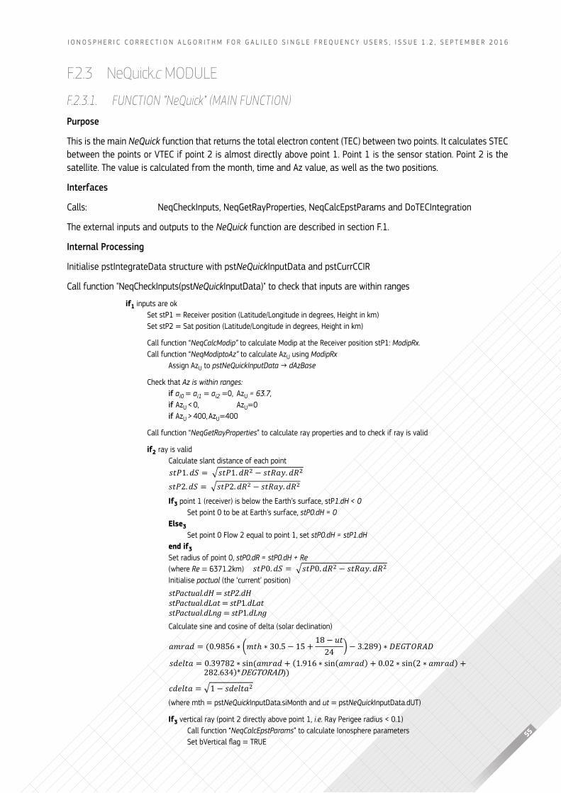
55


F.2.3 Nequick.c MODULE

f.2.3.1. fuNcTiON ”NeQuick” (main function)Purpose

this is the main NeQuick function that returns the total electron content (tec) between two points. It calculates stec between the points or vTEc if point 2 is almost directly above point 1. point 1 is the sensor station. point 2 is the satellite. the value is calculated from the month, time and Az value, as well as the two positions.

Interfaces

calls: neqcheckInputs, neqgetrayproperties, neqcalcepstparams and DotecIntegration

the external inputs and outputs to the NeQuick function are described in section f.1.

Internal Processing

Initialise pstIntegrateData structure with pstNeQuickInputData and pstcurrccIr

call function "neqcheckInputs(pstNeQuickInputData)" to check that inputs are within ranges

if1 inputs are okset stp1 = receiver position (latitude/longitude in degrees, height in km)set stp2 = sat position (latitude/longitude in degrees, height in km)

call function “NeqCalcModip” to calculate modip at the receiver position stp1: ModipRx.call function “NeqModiptoAz” to calculate Azu using ModipRx

Assign Azu to pstNeQuickinputData → dAzBase

check that Az is within ranges:if ai0 = ai1 = ai2 =0, Azu = 63.7,if Azu < 0, Azu=0if Azu > 400, Azu=400

call function “NeqGetRayProperties” to calculate ray properties and to check if ray is valid

if2 ray is validcalculate slant distance of each point

If3 point 1 (receiver) is below the earth’s surface, stp1�dH < 0set point 0 to be at earth’s surface, stP0.dH = 0

Else3 set point 0 flow 2 equal to point 1, set stP0.dH = stP1.dH

end if3set radius of point 0, stP0.dR = stP0.dH + Re(where Re = 6371.2km)Initialise pactual (the ‘current’ position)

calculate sine and cosine of delta (solar declination)

(where mth = pstNeQuickInputData.simonth and ut = pstNeQuickInputData.dut)

If3 vertical ray (point 2 directly above point 1, i�e� ray perigee radius < 0.1)call function “NeqCalcEpstParams” to calculate Ionosphere parametersSet bvertical flag = true

𝑠𝑠𝑠𝑠𝑠𝑠1. 𝑑𝑑𝑑𝑑 = √𝑠𝑠𝑠𝑠𝑠𝑠1. 𝑑𝑑𝑑𝑑2 − 𝑠𝑠𝑠𝑠𝑑𝑑𝑠𝑠𝑠𝑠. 𝑑𝑑𝑑𝑑2 𝑠𝑠𝑠𝑠𝑠𝑠2.𝑑𝑑𝑑𝑑 = �𝑠𝑠𝑠𝑠𝑠𝑠2.𝑑𝑑𝑑𝑑2 − 𝑠𝑠𝑠𝑠𝑑𝑑𝑠𝑠𝑠𝑠.𝑑𝑑𝑑𝑑2

𝑠𝑠𝑠𝑠𝑠𝑠0. 𝑑𝑑𝑑𝑑 = √𝑠𝑠𝑠𝑠𝑠𝑠0. 𝑑𝑑𝑑𝑑2 − 𝑠𝑠𝑠𝑠𝑑𝑑𝑠𝑠𝑠𝑠. 𝑑𝑑𝑑𝑑2

stPactual.dH = stP2.dHstPactual.dLat = stP1.dLatstPactual.dLng = stP1.dLng

𝑠𝑠𝑠𝑠𝑠𝑠𝑠𝑠𝑠𝑠𝑠𝑠 = 0.39782 ∗ sin (𝑠𝑠𝑎𝑎𝑎𝑎𝑠𝑠𝑠𝑠 + (1.916 ∗ sin(𝑠𝑠𝑎𝑎𝑎𝑎𝑠𝑠𝑠𝑠) + 0.02 ∗ sin(2 ∗ 𝑠𝑠𝑎𝑎𝑎𝑎𝑠𝑠𝑠𝑠) + 282.634) ∗ 𝐷𝐷𝐷𝐷𝐷𝐷𝐷𝐷𝐷𝐷𝐷𝐷𝐷𝐷𝐷𝐷)) 282.634)*DEGTORAD))

𝑎𝑎𝑎𝑎𝑎𝑎𝑎𝑎𝑎𝑎 = (0.9856 ∗ (𝑎𝑎𝑚𝑚ℎ ∗ 30.5 − 15 + 18 − 𝑢𝑢𝑚𝑚24 ) − 3.289) ∗ 𝐷𝐷𝐷𝐷𝐷𝐷𝐷𝐷𝐷𝐷𝐷𝐷𝐷𝐷𝐷𝐷

𝑐𝑐𝑐𝑐𝑐𝑐𝑐𝑐𝑐𝑐𝑐𝑐 = √1 − 𝑠𝑠𝑐𝑐𝑐𝑐𝑐𝑐𝑐𝑐𝑐𝑐2

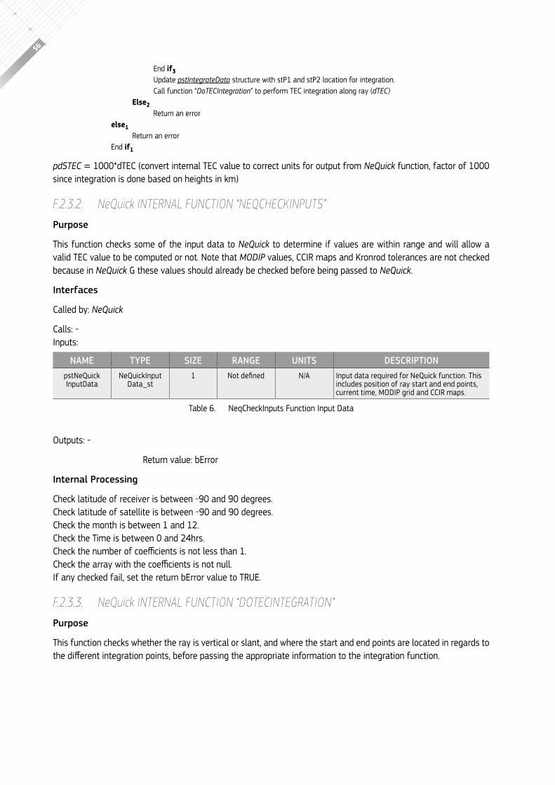
56

end if3update pstintegrateData structure with stp1 and stp2 location for integration.call function “DoTECIntegration” to perform tec integration along ray (dTEC)

Else2return an error

else1return an error

end if1

pdSTEC = 1000*dtec (convert internal tec value to correct units for output from NeQuick function, factor of 1000 since integration is done based on heights in km)

f.2.3.2. NeQuick iNTerNal fuNcTiON “NeQcheckiNPuTs”Purpose

this function checks some of the input data to NeQuick to determine if values are within range and will allow a valid tec value to be computed or not. note that MODiP values, ccIr maps and kronrod tolerances are not checked because in NeQuick g these values should already be checked before being passed to NeQuick.

Interfaces

called by: NeQuick

calls: -Inputs:

outputs: -

return value: berror

Internal Processing

check latitude of receiver is between -90 and 90 degrees.check latitude of satellite is between -90 and 90 degrees.check the month is between 1 and 12.check the time is between 0 and 24hrs.check the number of coefficients is not less than 1.check the array with the coefficients is not null.If any checked fail, set the return berror value to true.

f.2.3.3. NeQuick iNTerNal fuNcTiON “DOTeciNTeGraTiON”Purpose

this function checks whether the ray is vertical or slant, and where the start and end points are located in regards to the different integration points, before passing the appropriate information to the integration function.

NAmE tyPE SIzE RANGE UNItS DESCRIPtIONpstnequick InputData

nequickInput Data_st

1 not defined n/A Input data required for nequick function. this includes position of ray start and end points, current time, moDIp grid and ccIr maps.

table 6. neqcheckInputs function Input Data

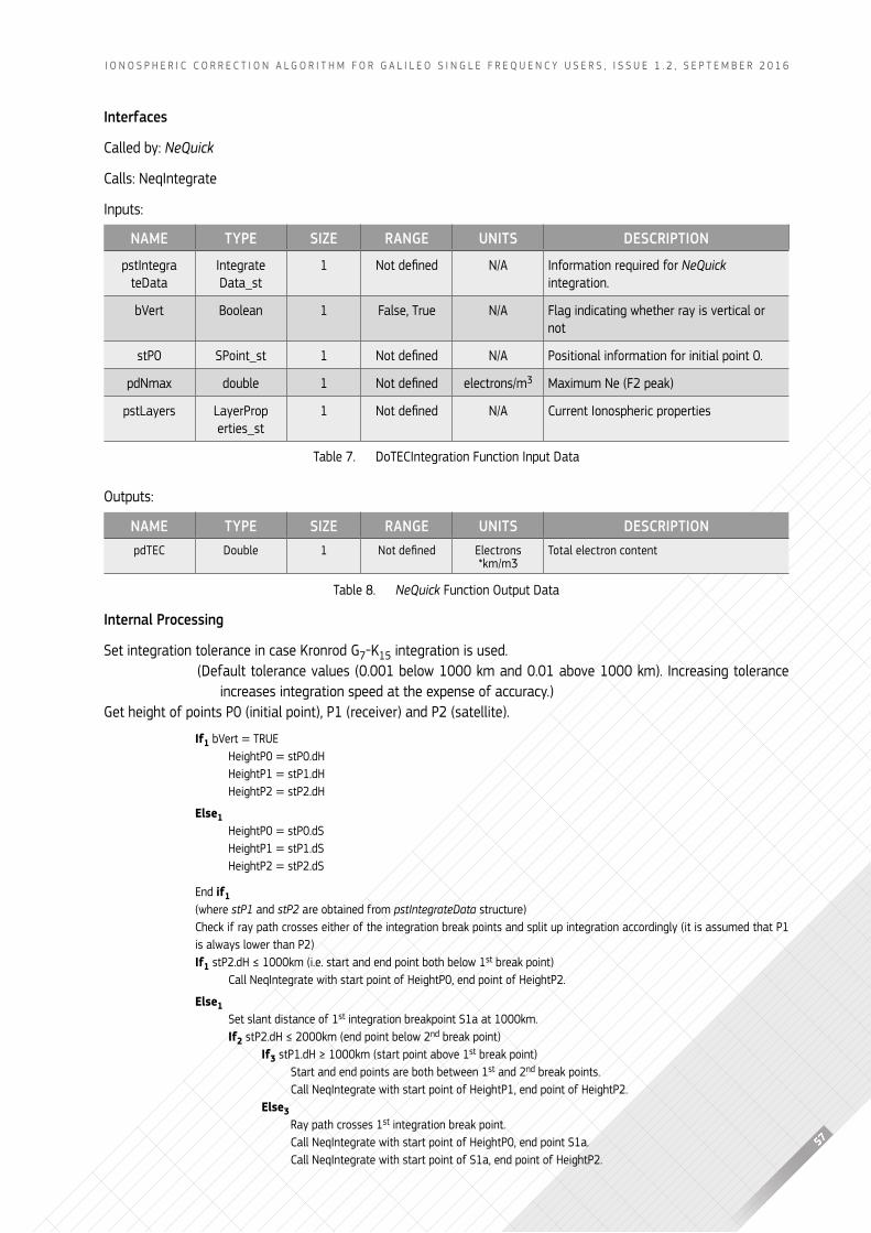
57


Interfaces

called by: NeQuick

calls: neqIntegrate

Inputs:

outputs:

Internal Processing

set integration tolerance in case kronrod g7-k15 integration is used. (Default tolerance values (0.001 below 1000 km and 0.01 above 1000 km). Increasing tolerance

increases integration speed at the expense of accuracy.)get height of points p0 (initial point), p1 (receiver) and p2 (satellite).

If1 bvert = trueheightp0 = stp0.dhheightp1 = stp1.dhheightp2 = stp2.dh

Else1heightp0 = stp0.dsheightp1 = stp1.dsheightp2 = stp2.ds

end if1(where stP1 and stP2 are obtained from pstintegrateData structure)check if ray path crosses either of the integration break points and split up integration accordingly (it is assumed that p1 is always lower than p2)If1 stp2.dh ≤ 1000km (i.e. start and end point both below 1st break point)

call neqIntegrate with start point of heightp0, end point of heightp2.

Else1set slant distance of 1st integration breakpoint s1a at 1000km.If2 stp2.dh ≤ 2000km (end point below 2nd break point)

If3 stp1.dh ≥ 1000km (start point above 1st break point)start and end points are both between 1st and 2nd break points.call neqIntegrate with start point of heightp1, end point of heightp2.

Else3 ray path crosses 1st integration break point. call neqIntegrate with start point of heightp0, end point s1a. call neqIntegrate with start point of s1a, end point of heightp2.

NAmE tyPE SIzE RANGE UNItS DESCRIPtION

pstIntegra teData

Integrate Data_st

1 not defined n/A Information required for NeQuick integration.

bvert boolean 1 false, true n/A flag indicating whether ray is vertical or not

stp0 spoint_st 1 not defined n/A positional information for initial point 0.

pdnmax double 1 not defined electrons/m3 maximum ne (f2 peak)

pstlayers layerprop erties_st

1 not defined n/A current Ionospheric properties

table 7. DotecIntegration function Input Data

NAmE tyPE SIzE RANGE UNItS DESCRIPtIONpdtec Double 1 not defined electrons

*km/m3total electron content


58

sum the tec values from the two neqIntegrate calls end if3

Else2If3 stp1.dh >= 2000km (start point above 2nd break point)

start and end points are both above 2nd break point.call neqIntegrate with start point of heightp1, end point of heightp2.

Else3 set slant distance of 2nd integration breakpoint s1b at 2000kmIf4 stp1.dh >= 1000km (start point above 1st break point)

ray path crosses 2nd integration break point. call neqIntegrate with start point of heightp1, end point of s1b. call neqIntegrate with start point of s1b, end point of heightp2.sum the tec values from the two neqIntegrate calls

Else4ray path crosses 1st and 2nd integration break points. call neqIntegrate with start point of heightp0, end point of s1a. call neqIntegrate with start point of s1a, end point of s1b. call neqIntegrate with start point of s1b, end point of heightp2.sum the tec values from the three neqIntegrate calls

end if4end if3

end if2end if1

F.2.4 neqcalcmodipaz.c MODULE

f.2.4.1. NeQuick iNTerNal fuNcTiON “NeQcalcMODiP”Purpose

This function uses the current latitude and longitude to calculate the corresponding modified dip latitude (MODiP) value. the MODiP grip should be ‘pre-wrapped’ at edges and poles.

Interfaces

called by: NeQuick, neqcalcepstparams

calls: neqInterpolate

Inputs:

return value: dreturn – calculated MODiP value at given location

Internal Processing

check latitude is within ±90 degrees

NAmE tyPE SIzE RANGE UNItS DESCRIPtIONdlat double 1 -90 to 90 deg latitude of point

dlng double 1 -180 to 180 deg longitude of point

pstmodip moDIp_st 1 not defined n/A Structure containing grid of modified dip latitude values.

table 9. neqcalcmodip function Input Data

59


if1 dlat ≤ -90set computed modip value dReturn = -90

else if1 dlat ≥ 90set computed modip value dReturn = 90

elseDefine properties of MODiP grid (lat step = 5 deg, lon step = 10 deg)constants describing grid lngp = 36,dlatp = 5,dlngp = 10

obtain lon grid square (sj) and position in that square (dj)

lng1 = (dLng + 180) / dlngpsj = floor(lng1) - 2dj=lng1 – floor(lng1)

Adjust for sign and wrap to grid if requiredIf2 (sj < 0)

sj = sj + lngpend if2if2 (sj > (lngp - 3))

sj = sj - lngp;end if2

obtain lat grid square (si) and position in that square (di)

lat1 = (dLat + 90) / dlatp + 1si = floor(lat1 - 1e-6) - 2di = lat1 - si - 2

Interpolate across lat grid to obtain values at 4 lon points on lat lineFor2 k = 1;k ≤ 4;++k

For3 j = 1;j ≤ 4;++jz1[j - 1] = pstmodip[si + j][sj + k + 1]

end for3z[k - 1] = neqInterpolate (z1,di)

end for2

Interpolate for lon value using these 4 points using neqInterpolate (z,dj);set computed modip value dReturn

end if1

f.2.4.2. NeQuick iNTerNal fuNcTiON “NeQiNTerPOlaTe”Purpose

This function performs third order interpolation. it is used when calculating the modified dip latitude value. input z [Annex A [4]] is -1,0,1,2 point values, x is position to interpolate to.

Interfaces

called by: neqcalcmodip

calls: none

Inputs:

NAmE tyPE SIzE RANGE UNItS DESCRIPtIONpdz double [Annex A

[4]]not defined n/A Array containing the -1, 0, 1 and 2 point values

dDeltax double 1 not defined n/A position to interpolate to (offset from 0pt to 1pt)

pstmodip moDIp_st 1 not defined n/A Structure containing grid of modified dip latitude values.

table 10. neqInterpolate function Input Data

60

return value: dIntz – the interpolated value at the point

Internal Processing

if1 dDeltax is small,return = zero point, pdz[1]1

else1Interpolate

g0 = pdZ[2] + pdZ[1]g1 = pdZ[2] - pdZ[1]g2 = pdZ[3] + pdZ[0]g3 = (pdZ[3] - pdZ[0]) / 3

a0 = 9*g0 - g2a1 = 9*g1 - g3a2 = g2 - g0a3 = g3 - g1

Δx = 2*dDeltax – 1

return =

end if1

f.2.4.3. NeQuick iNTerNal fuNcTiON “NeQMODiPTOaz”Purpose

This function calculates az from the provided coefficients and modified dip latitude value (μ). If only one non-zero coefficient (a0) is provided then Az = a0 (no dependency with MODiP). this function evaluates:

If Az < 0 then Az=0

Interfaces

called by: NeQuick

calls: none

Inputs:

return value: dFlx – the computed az value at the given modified dip latitude

Internal Processing

return (or zero if Az<0),

where:

i = sinumcoeff ai = pdcoeff μ = dmodip

116∑𝑎𝑎𝑗𝑗

3

𝑗𝑗=0∆𝑥𝑥𝑗𝑗

𝐴𝐴𝐴𝐴 =∑𝑎𝑎𝑖𝑖𝜇𝜇𝑖𝑖𝑖𝑖

NAmE tyPE SIzE RANGE UNItS DESCRIPtIONdmodip double 1 -90 to 90 deg modified dip latitude of point

sinumcoeff double 1 ≥1 n/A number of az coefficients

pdcoeff double [numcoeffs] >0 flux units/deg^j az coefficients

table 11. neqcalcmodip function Input Data

𝐴𝐴𝐴𝐴 =∑𝑎𝑎𝑖𝑖−1𝜇𝜇𝑖𝑖−1𝑖𝑖

61


F.2.5 neqGetraypropertieS.c MODULE

f.2.5.1. NeQuick iNTerNal fuNcTiON “NeQGeTrayPrOPerTies”Purpose

this function obtains the properties of the ray and checks if it is a valid ray. ‘ray’ is straight line passing through p1 and p2. pstRay→dLat, pstRay→dLng and pstRay→dR are co-ordinates of ray perigee, i.e. point on ray closest to centre of earth.

Interfaces

called by: main function

calls: neqcalcrayproperties1, neqcalcrayproperties2

Inputs/outputs:

outputs:

return value: berror – set to fAlse if no error and true if there is an error.

Internal Processing

check if ray is verticalif1 point 2 is directly above point 1, |pstP2→dLat – pstP1→dLat |<10-5 and | pstP2→dLng – pstP1→dLng |<10-5

set point 2 longitude to be exactly the same as point 1 longitude:pstP2→dLng = pstP1→dLng

end if1

calculate ranges of points 1 and 2 from the centre of the earthpstP1→dR = pstP1→dH + Re pstP2→dR = pstP2→dH + Re (Re = 6371.2km)

call function “neqcalcrayproperties1” to calculate properties of the ray itself.

if1 invalid ray, i.e. |pdZeta| > 90.0 and pstRay→dR < Reset return value berror to true

end if1

if1 ray is not vertical, pstRay→dR ≥ 0�1call function “neqcalcrayproperties2” to calculate additional ray properties.

end if1

return berror = fAlse

NAmE tyPE SIzE RANGE UNItS DESCRIPtIONpstp1 spoint_st 1 not defined n/A positional information for point 1 (receiver)

pstp2 spoint_st 1 not defined n/A positional information for point 2 (satellite)

table 12. neqgetrayproperties function Input/output Data

NAmE tyPE SIzE RANGE UNItS DESCRIPtIONpstray spoint_st 1 not defined n/A positional information for ray perigee

pdzeta double 1 -90 to 90 deg zenith angle of point 2 seen from point 1

pdsinsig double 1 -1 to 1 n/A sine of ray azimuth

pdcossig double 1 -1 to 1 n/A cosine of ray azimuth

table 13. neqgetrayproperties function output Data

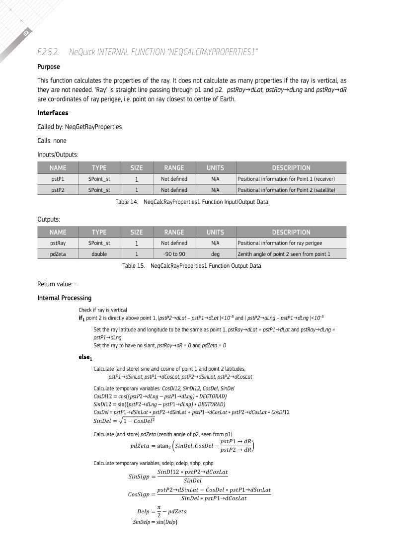
62

f.2.5.2. NeQuick iNTerNal fuNcTiON “NeQcalcrayPrOPerTies1”Purpose

this function calculates the properties of the ray. It does not calculate as many properties if the ray is vertical, as they are not needed. ‘ray’ is straight line passing through p1 and p2. pstRay→dLat, pstRay→dLng and pstRay→dR are co-ordinates of ray perigee, i.e. point on ray closest to centre of earth.

Interfaces

called by: neqgetrayproperties

calls: none

Inputs/outputs:

outputs:

return value: -

Internal Processing

check if ray is verticalif1 point 2 is directly above point 1, |pstP2→dLat – pstP1→dLat |<10-5 and | pstP2→dLng – pstP1→dLng |<10-5

set the ray latitude and longitude to be the same as point 1, pstray→dLat = pstP1→dLat and pstray→dLng = pstP1→dLngset the ray to have no slant, pstRay→dR = 0 and pdZeta = 0

else1

calculate (and store) sine and cosine of point 1 and point 2 latitudes, pstP1→dSinLat, pstP1→dCosLat, pstP2→dSinLat, pstP2→dCosLat

calculate temporary variables: CosDl12, SinDl12, CosDel, SinDelCosDl12 = cos((pstP2→dLng ― pstP1→dLng) * DEGTORAD)SinDl12 = sin((pstP2→dLng ― pstP1→dLng) * DEGTORAD)CosDel = pstP1→dSinLat * pstP2→dSinlat + pstP1→dCosLat * pstP2→dCosLat * CosDl12

calculate (and store) pdZeta (zenith angle of p2, seen from p1)

calculate temporary variables, sdelp, cdelp, sphp, cphp

SinDelp = sin(Delp)


pstp2 spoint_st 1 not defined n/A positional information for point 2 (satellite)

table 14. neqcalcrayproperties1 function Input/output Data


pdzeta double 1 -90 to 90 deg zenith angle of point 2 seen from point 1

table 15. neqcalcrayproperties1 function output Data

𝑆𝑆𝑆𝑆𝑆𝑆𝑆𝑆𝑆𝑆𝑆𝑆 = √1 − 𝐶𝐶𝐶𝐶𝐶𝐶𝑆𝑆𝑆𝑆𝑆𝑆2

𝑝𝑝𝑝𝑝𝑝𝑝𝑝𝑝𝑝𝑝𝑝𝑝 = atan2 (𝑆𝑆𝑆𝑆𝑆𝑆𝑆𝑆𝑝𝑝𝑆𝑆, 𝐶𝐶𝐶𝐶𝐶𝐶𝑆𝑆𝑝𝑝𝑆𝑆 −𝑝𝑝𝐶𝐶𝑝𝑝𝑝𝑝1 → 𝑝𝑝𝑑𝑑𝑝𝑝𝐶𝐶𝑝𝑝𝑝𝑝2 → 𝑝𝑝𝑑𝑑)

𝐶𝐶𝐶𝐶𝐶𝐶𝐶𝐶𝐶𝐶𝐶𝐶𝐶𝐶 = 𝐶𝐶𝐶𝐶𝑝𝑝𝑝𝑝2→𝑑𝑑𝐶𝐶𝐶𝐶𝑑𝑑𝑑𝑑𝑑𝑑𝑝𝑝 − 𝐶𝐶𝐶𝐶𝐶𝐶𝐶𝐶𝐶𝐶𝐶𝐶 ∗ 𝐶𝐶𝐶𝐶𝑝𝑝𝑝𝑝1→𝑑𝑑𝐶𝐶𝐶𝐶𝑑𝑑𝑑𝑑𝑑𝑑𝑝𝑝𝐶𝐶𝐶𝐶𝑑𝑑𝐶𝐶𝐶𝐶𝐶𝐶 ∗ 𝐶𝐶𝐶𝐶𝑝𝑝𝑝𝑝1→𝑑𝑑𝐶𝐶𝐶𝐶𝐶𝐶𝑑𝑑𝑑𝑑𝑝𝑝

𝑆𝑆𝑆𝑆𝑆𝑆𝑆𝑆𝑆𝑆𝑆𝑆𝑆𝑆 = 𝑆𝑆𝑆𝑆𝑆𝑆𝑆𝑆𝑆𝑆12 ∗ 𝑆𝑆𝑝𝑝𝑝𝑝𝑝𝑝2→𝑑𝑑𝑑𝑑𝑑𝑑𝑝𝑝𝑑𝑑𝑑𝑑𝑝𝑝𝑆𝑆𝑆𝑆𝑆𝑆𝑆𝑆𝑆𝑆𝑆𝑆

𝐷𝐷𝐷𝐷𝐷𝐷𝐷𝐷 = 𝜋𝜋2 − 𝐷𝐷𝑝𝑝𝑝𝑝𝐷𝐷𝑝𝑝𝑝𝑝

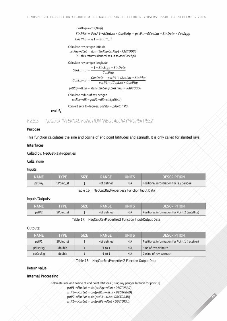
63


CosDelp = cos(Delp)

calculate ray perigee latitudepstRay→dLat = atan2(SinPhp,CosPhp) * RADTODEG

(nb this returns identical result to asin(SinPhp))

calculate ray perigee longitude

pstRay→dLng = atan2(SinLamp,CosLamp) * RADTODEG

calculate radius of ray perigeepstRay→dR = pstP1→dR * sin(pdZeta)

convert zeta to degrees, pdZeta = pdZeta * RDend if1

f.2.5.3. NeQuick iNTerNal fuNcTiON “NeQcalcrayPrOPerTies2"Purpose

this function calculates the sine and cosine of end point latitudes and azimuth. It is only called for slanted rays.

Interfaces

called by: neqgetrayproperties

calls: none

Inputs:

Inputs/outputs:

outputs:

return value: -

Internal Processing

calculate sine and cosine of end point latitudes (using ray perigee latitude for point 1)pstP1→dSinLat = sin(pstRay→dLat * DEGTORAD)pstP1→dCosLat = cos(pstRay→dLat * DEGTORAD)pstP2→dSinLat = sin(pstP2→dLat * DEGTORAD)pstP2→dCosLat = cos(pstP2→dLat * DEGTORAD)

𝑆𝑆𝑆𝑆𝑆𝑆𝑆𝑆ℎ𝑝𝑝 = 𝑆𝑆𝑃𝑃𝑃𝑃𝑆𝑆1→𝑑𝑑𝑆𝑆𝑆𝑆𝑆𝑆𝑑𝑑𝑑𝑑𝑃𝑃 ∗ 𝐶𝐶𝐶𝐶𝑃𝑃𝐶𝐶𝐶𝐶𝐶𝐶𝑝𝑝 − 𝑝𝑝𝑃𝑃𝑃𝑃𝑆𝑆1→𝑑𝑑𝐶𝐶𝐶𝐶𝑃𝑃𝑑𝑑𝑑𝑑𝑃𝑃 ∗ 𝑆𝑆𝑆𝑆𝑆𝑆𝐶𝐶𝐶𝐶𝐶𝐶𝑝𝑝 ∗ 𝐶𝐶𝐶𝐶𝑃𝑃𝑆𝑆𝑆𝑆𝐶𝐶𝑝𝑝 𝐶𝐶𝐶𝐶𝐶𝐶𝑃𝑃ℎ𝑝𝑝 = √1 − 𝑆𝑆𝑆𝑆𝑆𝑆𝑃𝑃ℎ𝑝𝑝2

𝑆𝑆𝑆𝑆𝑆𝑆𝑆𝑆𝑆𝑆𝑆𝑆𝑆𝑆 = −1 ∗ 𝑆𝑆𝑆𝑆𝑆𝑆𝑆𝑆𝑆𝑆𝑆𝑆𝑆𝑆 ∗ 𝑆𝑆𝑆𝑆𝑆𝑆𝑆𝑆𝑆𝑆𝑆𝑆𝑆𝑆𝐶𝐶𝐶𝐶𝐶𝐶𝐶𝐶ℎ𝑆𝑆

𝐶𝐶𝐶𝐶𝐶𝐶𝐶𝐶𝐶𝐶𝐶𝐶𝐶𝐶 = 𝐶𝐶𝐶𝐶𝐶𝐶𝐶𝐶𝐶𝐶𝐶𝐶𝐶𝐶 − 𝐶𝐶𝐶𝐶𝑝𝑝𝑝𝑝1→𝑑𝑑𝑑𝑑𝑑𝑑𝑑𝑑𝐶𝐶𝐶𝐶𝑝𝑝 ∗ 𝑑𝑑𝑑𝑑𝑑𝑑𝑝𝑝ℎ𝐶𝐶𝐶𝐶𝐶𝐶𝑝𝑝𝑝𝑝1→𝑑𝑑𝐶𝐶𝐶𝐶𝐶𝐶𝐶𝐶𝐶𝐶𝑝𝑝 ∗ 𝐶𝐶𝐶𝐶𝐶𝐶𝑝𝑝ℎ𝐶𝐶


table 16. neqcalcrayproperties2 function Input Data

NAmE tyPE SIzE RANGE UNItS DESCRIPtIONpstp2 spoint_st 1 not defined n/A positional information for point 2 (satellite)

table 17. neqcalcrayproperties2 function Input/output Data


pdsinsig double 1 -1 to 1 n/A sine of ray azimuth

pdcossig double 1 -1 to 1 n/A cosine of ray azimuth

table 18. neqcalcrayproperties2 function output Data

64

calculate difference in longitude of ray end pointsDeltaLong = (pstP2→dLng ― pstRay→dLng) * DEGTORAD

check if latitude of lower end point is ±90 degrees – would cause divide by zero error later onif1 ||pstRay→dLat| – 90| < 10-10

set sine of azimuth, pdSinSig = 0If2 positive latitude, pstRay→dLat > 0

set cosine of azimuth, pdCosSig = -1else2

set cosine of azimuth, pdCosSig = 1end if2

else1 calculate sine and cosine of angular distance between ends of ray (psi)

CosPsi = pstP1→dSinLat * pstP2→dSinLat + pstP1→dCosLat * pstP2→dCosLat * cos(DeltaLong)

calculate sine and cosine of azimuth

end if1

F.2.6 neqinteGrate.c MODULE

f.2.6.1. NeQuick iNTerNal fuNcTiON “NeQiNTeGraTe”Purpose

Integration function for calculating tec along rays using kronrod g7-k15 adaptive quadrature method. this method involves sampling values at 15 points and calculating the integration from them. At the same time it misses out half of the points to see what difference it makes and therefore the likely error contained in the result, before deciding whether to accept the result, or to split the portion into two and try again in order to improve accuracy.

note that this method is recursive but has appropriate safeguards in the form of the recursion limit passed in from configuration.

Interfaces

called by: DotecIntegration

calls: self (recursive), neqGetneonvertray, neqGetneonSlantray

Inputs:

outputs:

𝑆𝑆𝑆𝑆𝑆𝑆𝑆𝑆𝑆𝑆𝑆𝑆 = √1 − 𝐶𝐶𝐶𝐶𝑆𝑆𝑆𝑆𝑆𝑆𝑆𝑆2

𝑝𝑝𝑝𝑝𝑝𝑝𝑝𝑝𝑝𝑝𝑝𝑝𝑝𝑝𝑝𝑝 = 𝑝𝑝𝑝𝑝𝑝𝑝𝑝𝑝2→𝑝𝑝𝑑𝑑𝑑𝑑𝑝𝑝𝑑𝑑𝑑𝑑𝑝𝑝 ∗ sin(𝐷𝐷𝐷𝐷𝐷𝐷𝑝𝑝𝑑𝑑𝑑𝑑𝑑𝑑𝑝𝑝𝑝𝑝)𝑝𝑝𝑝𝑝𝑝𝑝𝑝𝑝𝑝𝑝𝑝𝑝

𝑝𝑝𝑝𝑝𝑝𝑝𝑝𝑝𝑝𝑝𝑝𝑝𝑝𝑝𝑝𝑝 = 𝑝𝑝𝑝𝑝𝑝𝑝𝑝𝑝2→𝑝𝑝𝑝𝑝𝑝𝑝𝑑𝑑𝑑𝑑𝑑𝑑𝑝𝑝 − 𝑝𝑝𝑝𝑝𝑝𝑝𝑝𝑝1→𝑝𝑝𝑝𝑝𝑝𝑝𝑑𝑑𝑑𝑑𝑑𝑑𝑝𝑝 ∗ 𝑝𝑝𝑝𝑝𝑝𝑝𝑝𝑝𝑝𝑝𝑝𝑝𝑝𝑝𝑝𝑝𝑑𝑑𝑝𝑝𝑝𝑝𝑝𝑝 ∗ 𝑝𝑝𝑝𝑝𝑝𝑝𝑝𝑝1→𝑝𝑝𝑝𝑝𝑝𝑝𝑝𝑝𝑑𝑑𝑑𝑑𝑝𝑝

NAmE tyPE SIzE RANGE UNItS DESCRIPtIONpstIntegrateData IntegrateData_st 1 not defined n/A Data required for computation of integrated

tec value

dh1 double 1 not defined km height of point 1

dh2 double 1 not defined km height of point 2

sicurrentlevel Integer 1 ≥0 n/A current level of integration recursion

table 19. neqIntegrate function Input Data

NAmE tyPE SIzE RANGE UNItS DESCRIPtIONpstpactual spoint_st 1 not defined n/A positional information for current integration

point.

table 20. neqIntegrate function output Data

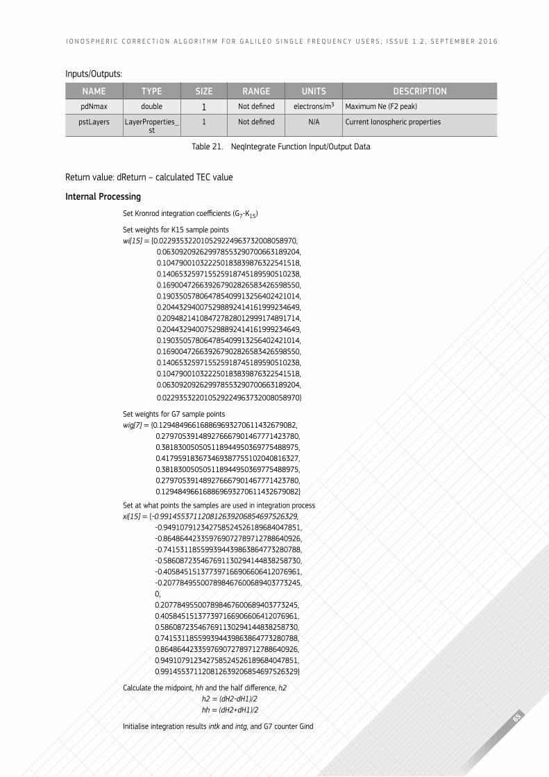
65


Inputs/outputs:

return value: dreturn – calculated tec value

Internal Processing

Set Kronrod integration coefficients (G7-k15)

set weights for k15 sample pointswi[15] = {0.022935322010529224963732008058970,

0.063092092629978553290700663189204, 0.104790010322250183839876322541518, 0.140653259715525918745189590510238, 0.169004726639267902826583426598550, 0.190350578064785409913256402421014, 0.204432940075298892414161999234649, 0.209482141084727828012999174891714, 0.204432940075298892414161999234649, 0.190350578064785409913256402421014, 0.169004726639267902826583426598550, 0.140653259715525918745189590510238, 0.104790010322250183839876322541518, 0.063092092629978553290700663189204,

0.022935322010529224963732008058970}

set weights for g7 sample pointswig[7] = {0.129484966168869693270611432679082,

0.279705391489276667901467771423780, 0.381830050505118944950369775488975, 0.417959183673469387755102040816327, 0.381830050505118944950369775488975, 0.279705391489276667901467771423780, 0.129484966168869693270611432679082}

set at what points the samples are used in integration processxi[15] = {-0.991455371120812639206854697526329,

-0.949107912342758524526189684047851, -0.864864423359769072789712788640926, -0.741531185599394439863864773280788, -0.586087235467691130294144838258730, -0.405845151377397166906606412076961, -0.207784955007898467600689403773245, 0, 0.207784955007898467600689403773245, 0.405845151377397166906606412076961, 0.586087235467691130294144838258730, 0.741531185599394439863864773280788, 0.864864423359769072789712788640926, 0.949107912342758524526189684047851, 0.991455371120812639206854697526329}

calculate the midpoint, hh and the half difference, h2h2 = (dH2-dH1)/2hh = (dH2+dH1)/2

Initialise integration results intk and intg, and g7 counter gind

NAmE tyPE SIzE RANGE UNItS DESCRIPtIONpdnmax double 1 not defined electrons/m3 maximum ne (f2 peak)

pstlayers layerproperties_st


table 21. neqIntegrate function Input/output Data

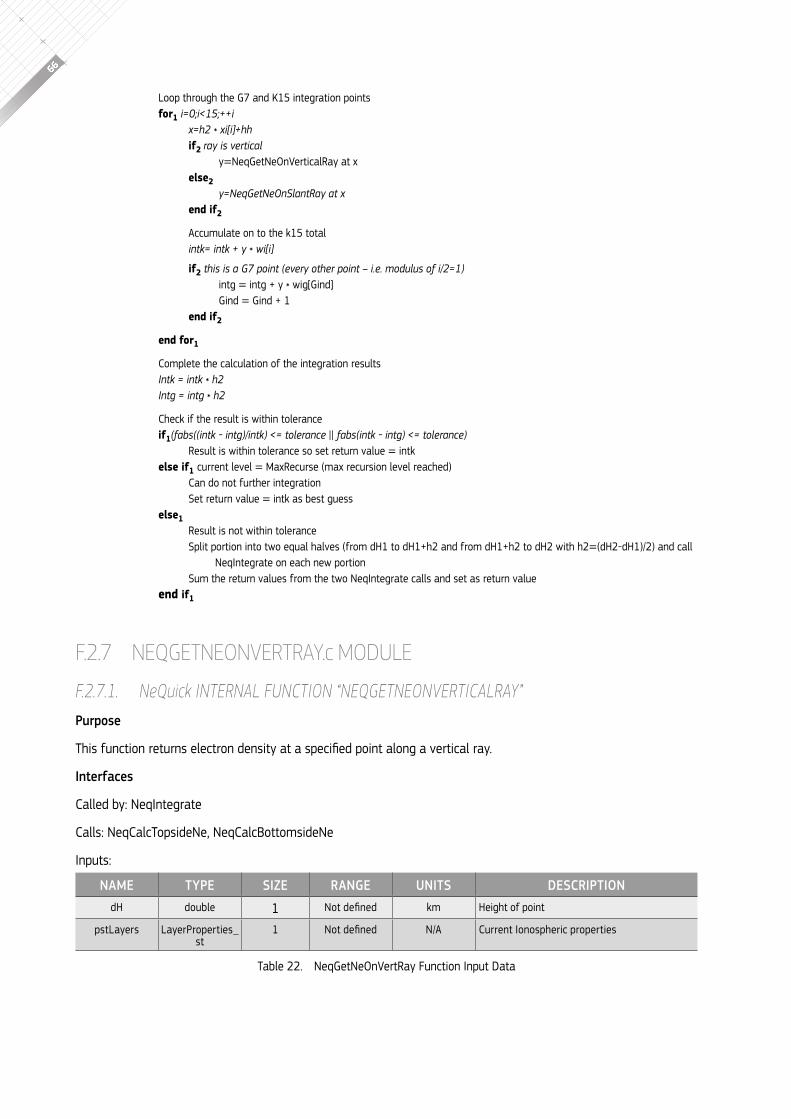
66

loop through the g7 and k15 integration pointsfor1 i=0;i<15;++i

x=h2 * xi[i]+hhif2 ray is vertical

y=neqGetneonverticalray at x else2

y=NeqGetNeOnSlantRay at xend if2

Accumulate on to the k15 totalintk= intk + y * wi[i]

if2 this is a G7 point (every other point – i.e. modulus of i/2=1)intg = intg + y * wig[gind]gind = Gind + 1

end if2

end for1

complete the calculation of the integration resultsIntk = intk * h2Intg = intg * h2

check if the result is within toleranceif1(fabs((intk - intg)/intk) <= tolerance || fabs(intk - intg) <= tolerance)

result is within tolerance so set return value = intk else if1 current level = maxrecurse (max recursion level reached)

can do not further integrationset return value = intk as best guess

else1result is not within toleranceSplit portion into two equal halves (from dh1 to dh1+h2 and from dh1+h2 to dh2 with h2=(dh2-dh1)/2) and call

neqIntegrate on each new portionsum the return values from the two neqIntegrate calls and set as return value

end if1

F.2.7 neqGetneonvertray.c MODULE

f.2.7.1. NeQuick iNTerNal fuNcTiON “NeQGeTNeONverTicalray”Purpose

This function returns electron density at a specified point along a vertical ray.

Interfaces

called by: neqIntegrate

calls: neqcalctopsidene, neqcalcbottomsidene

Inputs:

NAmE tyPE SIzE RANGE UNItS DESCRIPtIONdh double 1 not defined km height of point



table 22. neqGetneonvertray Function input Data

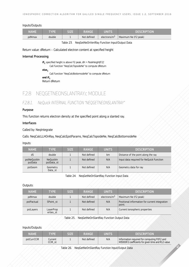
67


Inputs/outputs:

return value: dreturn – calculated electron content at specified height

Internal Processing

if1 specified height is above F2 peak, dh > PeakHeight[F2]call function “NeqCalcTopsideNe” to compute dreturn

else1 call function “NeqCalcBottomsideNe” to compute dreturn

end if1return dreturn

F.2.8 neqGetneonSlantray.c MODULE

f.2.8.1. NeQuick iNTerNal fuNcTiON “NeQGeTNeONslaNTray”Purpose

This function returns electron density at the specified point along a slanted ray.

Interfaces

called by: neqIntegrate

calls: neqcalcllhonray, neqcalcepstparams, neqcalctopsidene, neqcalcbottomsidene

Inputs:

outputs:

Inputs/outputs:


table 23. neqGetneonvertray Function input/output Data

NAmE tyPE SIzE RANGE UNItS DESCRIPtIONds double 1 not defined km Distance of the point along the ray

pstnequickIn putData

nequickIn putData_st

1 not defined n/A Input data required for nequick function

pstgeom geometry Data_st

1 not defined n/A geometry data for ray

table 24. neqgetneonslantray function Input Data


pstpactual spoint_st 1 not defined n/A positional information for current integration point.

pstlayers layerprop erties_st


table 25. neqgetneonslantray function output Data

NAmE tyPE SIzE RANGE UNItS DESCRIPtIONpstcurrccIr current

ccIr_st1 not defined n/A Information required for computing f0f2 and

m3000F2 coefficients for given time and r12 value.

table 26. neqgetneonslantray function Input/output Data

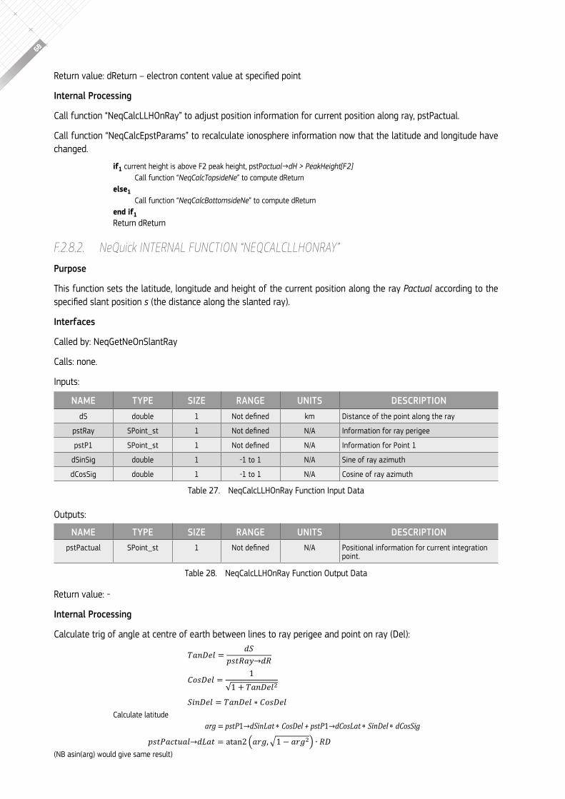
68

return value: dreturn – electron content value at specified point

Internal Processing

call function “neqcalcllhonray” to adjust position information for current position along ray, pstpactual.

call function “neqcalcepstparams” to recalculate ionosphere information now that the latitude and longitude have changed.

if1 current height is above f2 peak height, pstpactual→dH > PeakHeight[F2]call function “NeqCalcTopsideNe” to compute dreturn

else1 call function “NeqCalcBottomsideNe” to compute dreturn

end if1return dreturn

f.2.8.2. NeQuick iNTerNal fuNcTiON “NeQcalcllhONray”Purpose

this function sets the latitude, longitude and height of the current position along the ray Pactual according to the specified slant position s (the distance along the slanted ray).

Interfaces

called by: neqgetneonslantray

calls: none.

Inputs:

outputs:

return value: -

Internal Processing

calculate trig of angle at centre of earth between lines to ray perigee and point on ray (Del):

calculate latitudearg = pstP1→dSinLat ∗ CosDel + pstP1→dCosLat ∗ SinDel ∗ dCosSig

(nb asin(arg) would give same result)

NAmE tyPE SIzE RANGE UNItS DESCRIPtIONds double 1 not defined km Distance of the point along the ray

pstray spoint_st 1 not defined n/A Information for ray perigee

pstp1 spoint_st 1 not defined n/A Information for point 1

dsinsig double 1 -1 to 1 n/A sine of ray azimuth

dcossig double 1 -1 to 1 n/A cosine of ray azimuth

table 27. neqcalcllhonray function Input Data

NAmE tyPE SIzE RANGE UNItS DESCRIPtIONpstpactual spoint_st 1 not defined n/A positional information for current integration

point.

table 28. neqcalcllhonray function output Data

𝑇𝑇𝑇𝑇𝑇𝑇𝑇𝑇𝑇𝑇𝑇𝑇 = 𝑑𝑑𝑑𝑑𝑝𝑝𝑝𝑝𝑝𝑝𝑝𝑝𝑇𝑇𝑝𝑝→𝑑𝑑𝑝𝑝

𝐶𝐶𝐶𝐶𝑝𝑝𝑇𝑇𝑇𝑇𝑇𝑇 = 1√1 + 𝑇𝑇𝑇𝑇𝑇𝑇𝑇𝑇𝑇𝑇𝑇𝑇2

𝑑𝑑𝑆𝑆𝑇𝑇𝑇𝑇𝑇𝑇𝑇𝑇 = 𝑇𝑇𝑇𝑇𝑇𝑇𝑇𝑇𝑇𝑇𝑇𝑇 ∗ 𝐶𝐶𝐶𝐶𝑝𝑝𝑇𝑇𝑇𝑇𝑇𝑇

𝑝𝑝𝑝𝑝𝑝𝑝𝑝𝑝𝑝𝑝𝑝𝑝𝑝𝑝𝑝𝑝𝑝𝑝𝑝𝑝→𝑑𝑑𝑑𝑑𝑝𝑝𝑝𝑝 = atan2 (𝑝𝑝𝑎𝑎𝑎𝑎,√1 − 𝑝𝑝𝑎𝑎𝑎𝑎2) ∙ 𝑅𝑅𝑅𝑅

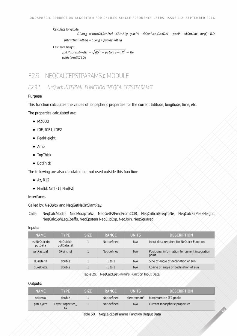
69


calculate longitude

pstPactual→dLng = CLong + pstRay→dLng

calculate height𝑝𝑝𝑝𝑝𝑝𝑝𝑝𝑝𝑝𝑝𝑝𝑝𝑝𝑝𝑝𝑝𝑝𝑝𝑝𝑝→𝑑𝑑𝑑𝑑 = √𝑑𝑑𝑑𝑑2 + 𝑝𝑝𝑝𝑝𝑝𝑝𝑝𝑝𝑝𝑝𝑝𝑝→𝑑𝑑𝑝𝑝2 − 𝑝𝑝𝑅𝑅 (with re=6371.2)

F.2.9 neqcalcepStparamS.c MODULE

f.2.9.1. NeQuick iNTerNal fuNcTiON “NeQcalcePsTParaMs”Purpose

this function calculates the values of ionospheric properties for the current latitude, longitude, time, etc.

the properties calculated are:

● m3000

● f0e, f0f1, f0f2

● peakheight

● Amp

● topthick

● botthick

the following are also calculated but not used outside this function:

● Az, r12,

● nm[e], nm[f1], nm[f2]

Interfaces

called by: NeQuick and neqgetneonslantray.

calls: neqcalcmodip, neqmodiptoAz, neqgetf2freqfromccIr, neqcriticalfreqtone, neqcalcf2peakheight, neqcalcSphlegcoeffs, neqEpstein neqclipExp, neqJoin, neqSquared

Inputs:

outputs:

𝐶𝐶𝐶𝐶𝐶𝐶𝐶𝐶𝐶𝐶 = atan2(𝑆𝑆𝑆𝑆𝐶𝐶𝑆𝑆𝑆𝑆𝑆𝑆 ∙ 𝑑𝑑𝑆𝑆𝑆𝑆𝐶𝐶𝑆𝑆𝑆𝑆𝐶𝐶 ∙ 𝑝𝑝𝑝𝑝𝑝𝑝𝑝𝑝1→𝑑𝑑𝐶𝐶𝐶𝐶𝑝𝑝𝐶𝐶𝑑𝑑𝑝𝑝, 𝐶𝐶𝐶𝐶𝑝𝑝𝑆𝑆𝑆𝑆𝑆𝑆 − 𝑝𝑝𝑝𝑝𝑝𝑝𝑝𝑝1→𝑑𝑑𝑆𝑆𝑆𝑆𝐶𝐶𝐶𝐶𝑑𝑑𝑝𝑝 ∙ 𝑑𝑑𝑎𝑎𝐶𝐶) ∙ 𝑅𝑅𝑆𝑆

NAmE tyPE SIzE RANGE UNItS DESCRIPtIONpstnequickIn

putDatanequickIn putData_st

1 not defined n/A Input data required for nequick function

pstpactual spoint_st 1 not defined n/A positional information for current integration point.

dsinDelta double 1 -1 to 1 n/A sine of angle of declination of sun

dcosDelta double 1 -1 to 1 n/A cosine of angle of declination of sun

table 29. neqcalcepstparams function Input Data




table 30. neqcalcepstparams function output Data

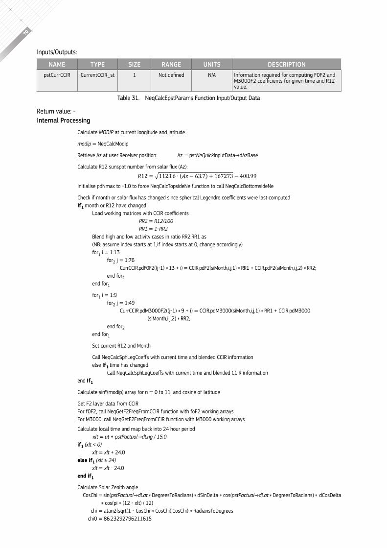
70

Inputs/outputs:

return value: -Internal Processing

calculate MODiP at current longitude and latitude.

modip = neqcalcmodip

retrieve Az at user receiver position: Az = pstNeQuickInputData→dAzbase

calculate r12 sunspot number from solar flux (az):

Initialise pdnmax to -1.0 to force neqcalctopsidene function to call neqcalcbottomsidene

check if month or solar flux has changed since spherical legendre coefficients were last computedIf1 month or r12 have changed

load working matrices with ccir coefficientsRR2 = R12/100RR1 = 1-RR2

blend high and low activity cases in ratio rr2:rr1 as (nb: assume index starts at 1,if index starts at 0, change accordingly)for1 i = 1:13

for2 j = 1:76currccIr.pdf0f2((j-1) * 13 + i) = ccIr.pdf2(simonth,i,j,1) * rr1 + ccir.pdF2(simonth,i,j,2) * rr2;

end for2end for1

for1 i = 1:9for2 j = 1:49

currccIr.pdm3000f2((j-1) * 9 + i) = ccIr.pdm3000(simonth,i,j,1) * rr1 + ccir.pdm3000 (simonth,i,j,2) * rr2;

end for2end for1

set current r12 and month

call neqcalcSphlegcoeffs with current time and blended ccir informationelse If1 time has changed

call neqcalcSphlegcoeffs with current time and blended ccir informationend If1

calculate sinn(modip) array for n = 0 to 11, and cosine of latitude

get f2 layer data from ccIr for f0f2, call neqgetf2freqfromccIr function with fof2 working arraysfor m3000, call neqgetf2freqfromccIr function with m3000 working arrays

calculate local time and map back into 24 hour periodxlt = ut + pstPactual→dLng / 15.0

if1 (xlt < 0)xlt = xlt + 24.0

else if1 (xlt ≥ 24)xlt = xlt - 24.0

end if1

calculate solar zenith anglecoschi = sin(pstPactual→dLat * Degreestoradians) * dSinDelta + cos(pstPactual→dLat * Degreestoradians) * dcosDelta

* cos(pi * (12 - xlt) / 12)chi = atan2(sqrt(1 - coschi * coschi),coschi) * radianstoDegrees

chi0 = 86.23292796211615



table 31. neqcalcepstparams function Input/output Data

𝑅𝑅12 = √1123.6 ∙ (𝐴𝐴𝐴𝐴 − 63.7) + 167273 − 408.99

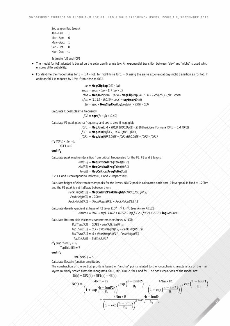
71


Set season flag (seas):jan – feb: -1mar – Apr: 0may – Aug: 1sep – oct: 0nov – Dec: -1

estimate foe and f0f1 ● the model for foe adopted is based on the solar zenith angle law. An exponential transition between “day” and “night” is used which

ensures differentiability.

● for daytime the model takes fof1 = 1.4 * foe, for night-time fof1 = 0, using the same exponential day-night transition as for foe. In addition foF1 is reduced by 15% if too close to foF2.

ee = NeqClipExp(0�3 * lat)seas = seas * (ee - 1) / (ee + 1)chin = NeqJoin(90.0 - 0.24 * NeqClipExp(20�0 - 0�2 * chi),chi,12,chi - chi0)sfac = (1�112 - 0.019 * seas) * sqrt(sqrt(Az))

fa = sfac * NeqClipExp(log(cos(chin * DR)) * 0�3)

calculate e peak plasma frequencyf0e = sqrt(fa * fa + 0.49)

calculate f1 peak plasma frequency and set to zero if negligiblef0F1 = NeqJoin(1.4 * f0e,0,1000�0,f0e - 2) (titheridge’s formula f0f1 = 1.4 f0f2)f0F1 = NeqJoin(0,f0F1,1000�0,f0e - f0F1)f0F1 = NeqJoin(f0F1,0.85 * f0F1,60.0,0.85 * f0F2 - f0F1)

if1 (f0F1 < 1e - 6)f0f1 = 0

end if1

calculate peak electron densities from critical frequencies for the f2, f1 and e layers.Nm[F2] = NeqCriticalFreqToNe(foF2)Nm[F1] = NeqCriticalFreqToNe(foF1)Nm[e] = NeqCriticalFreqToNe(foe)

(f2, f1 and e correspond to indices 0, 1 and 2 respectively)

calculate height of electron density peaks for the layers. nb F2 peak is calculated each time, E layer peak is fixed at 120km and the f1 peak is set halfway between them.

PeakHeight[F2] = NeqCalcF2PeakHeight(M3000, foe, foF2)PeakHeight[e] = 120km

PeakHeight[F1] = (PeakHeight[F2] + PeakHeight[e]) / 2

calculate density gradient at base of f2 layer (109 m-3 km-1) (see Annex A [12])NdHmx = 0�01 * exp(-3.467 + 0.857 * log(f0F2 * f0F2) + 2�02 * log(M3000))

calculate bottom-side thickness parameters (see Annex A [13])BotThick[F2] = 0.385 * Nm[F2] / NdHmxTopThick[F1] = 0�3 * (PeakHeight[F2] – PeakHeight[F1])BotThick[F1] = �5 * (PeakHeight[F1] – PeakHeight[e])TopThick[E] = BotThick[F1]

if1 (TopThick[E] < 7)topthick[e] = 7

end if1BotThick[E] = 5

calculate epstein function amplitudesThe construction of the vertical profile is based on “anchor” points related to the ionospheric characteristics of the main layers routinely scaled from the ionograms: fof2, m(3000)f2, fof1 and foe. the basic equations of the model are:

N(h) = NF2(h) + NF1(h) + NE(h)

N(h) = 4Nm ∗ F2

(1 + exp (h − hmF2B2 ))

2 exp (h − hmF2

B2) + 4Nm ∗ F1

(1 + exp (h − hmF1B1 ))

2 exp (h − hmF1

B1)

+ 4Nm ∗ E

(1 + exp (h − hmEBE ))

2 exp (h − hmE

BE)

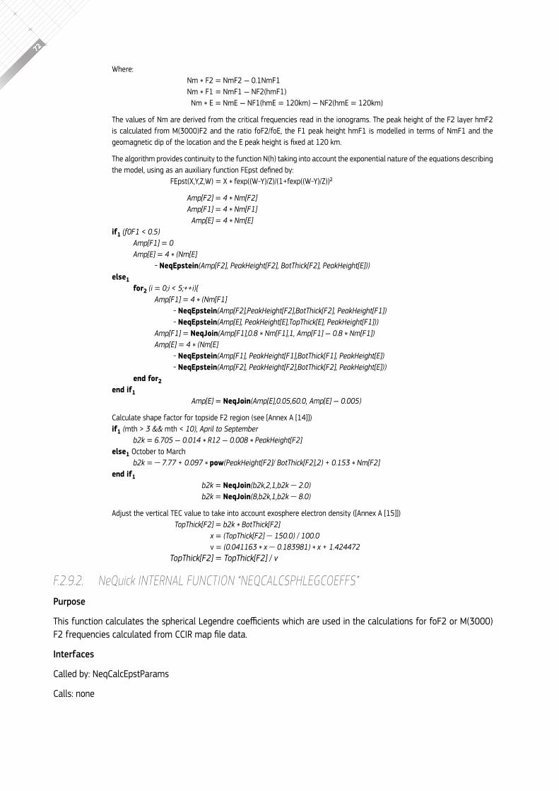
72

where:nm * f2 = nmf2 ― 0.1nmf1nm * f1 = nmf1 ― nf2(hmf1)nm * e = nme ― nf1(hme = 120km) ― nf2(hme = 120km)

the values of nm are derived from the critical frequencies read in the ionograms. the peak height of the f2 layer hmf2 is calculated from m(3000)f2 and the ratio fof2/foe, the f1 peak height hmf1 is modelled in terms of nmf1 and the geomagnetic dip of the location and the E peak height is fixed at 120 km.

the algorithm provides continuity to the function n(h) taking into account the exponential nature of the equations describing the model, using as an auxiliary function FEpst defined by:

fepst(x,y,z,w) = x * fexp((w-y)/Z)/(1+fexp((w-y)/Z))²

Amp[F2] = 4 * Nm[F2]Amp[F1] = 4 * Nm[F1]

Amp[e] = 4 * Nm[e]if1 (f0F1 < 0�5)

Amp[F1] = 0Amp[e] = 4 * (Nm[e]

- NeqEpstein(Amp[F2], PeakHeight[F2], BotThick[F2], PeakHeight[E]))else1

for2 (i = 0;i < 5;++i){Amp[F1] = 4 * (Nm[F1]

- NeqEpstein(Amp[F2],PeakHeight[F2],BotThick[F2], PeakHeight[F1]) - NeqEpstein(Amp[E], PeakHeight[E],TopThick[E], PeakHeight[F1]))

Amp[F1] = NeqJoin(Amp[F1],0.8 * Nm[F1],1, Amp[F1] ― 0.8 * Nm[F1])Amp[e] = 4 * (Nm[e]

- NeqEpstein(Amp[F1], PeakHeight[F1],BotThick[F1], PeakHeight[E]) - NeqEpstein(Amp[F2], PeakHeight[F2],BotThick[F2], PeakHeight[E]))

end for2end if1

Amp[e] = NeqJoin(Amp[e],0�05,60�0, Amp[e] ― 0�005)

calculate shape factor for topside f2 region (see [Annex A [14]])if1 (mth > 3 && mth < 10), April to September

b2k = 6�705 ― 0.014 * R12 ― 0.008 * PeakHeight[F2]else1 october to march

b2k = ― 7�77 + 0.097 * pow(PeakHeight[F2]/ BotThick[F2],2) + 0�153 * Nm[F2]end if1

b2k = NeqJoin(b2k,2,1,b2k ― 2�0)b2k = NeqJoin(8,b2k,1,b2k ― 8.0)

Adjust the vertical tec value to take into account exosphere electron density ([Annex A [15]])TopThick[F2] = b2k * BotThick[F2]

x = (TopThick[F2] ― 150�0) / 100�0v = (0.041163 * x ― 0.183981) * x + 1.424472

TopThick[F2] = TopThick[F2] / v

f.2.9.2. NeQuick iNTerNal fuNcTiON “NeQcalcsPhleGcOeffs”Purpose

This function calculates the spherical legendre coefficients which are used in the calculations for foF2 or m(3000)F2 frequencies calculated from ccir map file data.

Interfaces

called by: neqcalcepstparams

calls: none

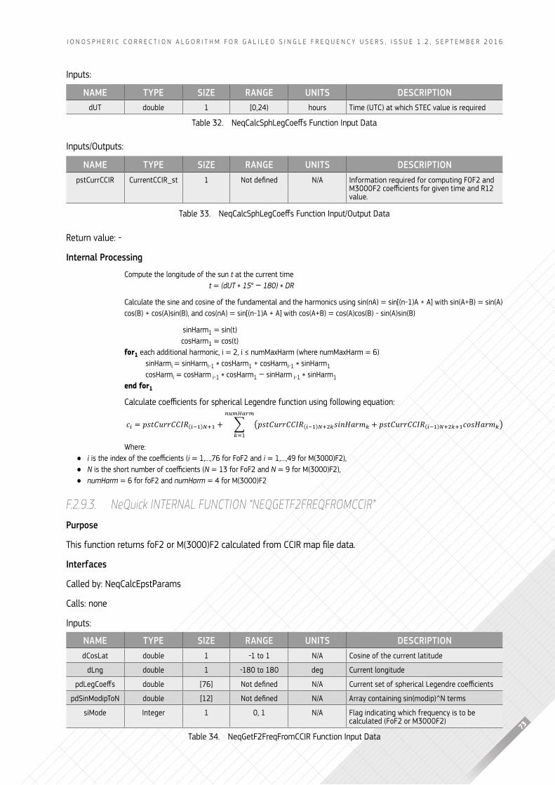
73


Inputs:

Inputs/outputs:

return value: -

Internal Processing

compute the longitude of the sun t at the current timet = (dUT * 15° ― 180) * DR

calculate the sine and cosine of the fundamental and the harmonics using sin(nA) = sin[(n-1)a + a] with sin(a+b) = sin(A)cos(b) + cos(a)sin(b), and cos(na) = sin[(n-1)a + a] with cos(a+b) = cos(A)cos(b) - sin(A)sin(b)

sinharm1 = sin(t)cosharm1 = cos(t)

for1 each additional harmonic, i = 2, i ≤ nummaxharm (where nummaxharm = 6)sinharmi = sinharmi-1 * cosharm1 + cosharmi-1 * sinharm1cosharmi = cosharm i-1 * cosharm1 ― sinharm i-1 * sinharm1

end for1

calculate coefficients for spherical legendre function using following equation:

where: ● i is the index of the coefficients (i = 1,…,76 for fof2 and i = 1,…,49 for m(3000)f2), ● N is the short number of coefficients (N = 13 for fof2 and N = 9 for m(3000)f2), ● numHarm = 6 for fof2 and numHarm = 4 for m(3000)f2

f.2.9.3. NeQuick iNTerNal fuNcTiON “NeQGeTf2freQfrOMccir”Purpose

This function returns foF2 or m(3000)F2 calculated from ccir map file data.

Interfaces


calls: none

Inputs:

NAmE tyPE SIzE RANGE UNItS DESCRIPtIONdut double 1 [0,24) hours time (utc) at which stec value is required

table 32. neqcalcSphlegcoeffs Function input Data



table 33. neqcalcSphlegcoeffs Function input/output Data

𝑐𝑐𝑖𝑖 = 𝑝𝑝𝑝𝑝𝑝𝑝𝑝𝑝𝑝𝑝𝑝𝑝𝑝𝑝𝑝𝑝𝑝𝑝𝑝𝑝𝑝𝑝(𝑖𝑖−1)𝑁𝑁+1 + ∑ (𝑝𝑝𝑝𝑝𝑝𝑝𝑝𝑝𝑝𝑝𝑝𝑝𝑝𝑝𝑝𝑝𝑝𝑝𝑝𝑝𝑝𝑝(𝑖𝑖−1)𝑁𝑁+2𝑘𝑘𝑝𝑝𝑠𝑠𝑠𝑠𝑠𝑠𝑠𝑠𝑝𝑝𝑠𝑠𝑘𝑘 + 𝑝𝑝𝑝𝑝𝑝𝑝𝑝𝑝𝑝𝑝𝑝𝑝𝑝𝑝𝑝𝑝𝑝𝑝𝑝𝑝𝑝𝑝(𝑖𝑖−1)𝑁𝑁+2𝑘𝑘+1𝑐𝑐𝑐𝑐𝑝𝑝𝑠𝑠𝑠𝑠𝑝𝑝𝑠𝑠𝑘𝑘)𝑛𝑛𝑛𝑛𝑛𝑛𝑛𝑛𝑛𝑛𝑛𝑛𝑛𝑛

𝑘𝑘=1

NAmE tyPE SIzE RANGE UNItS DESCRIPtIONdcoslat double 1 -1 to 1 n/A cosine of the current latitude

dlng double 1 -180 to 180 deg current longitude

pdlegcoeffs double [76] not defined n/A current set of spherical legendre coefficients

pdsinmodipton double [12] not defined n/A array containing sin(modip)^n terms

simode Integer 1 0, 1 n/A flag indicating which frequency is to be calculated (fof2 or m3000f2)

table 34. neqgetf2freqfromccIr function Input Data

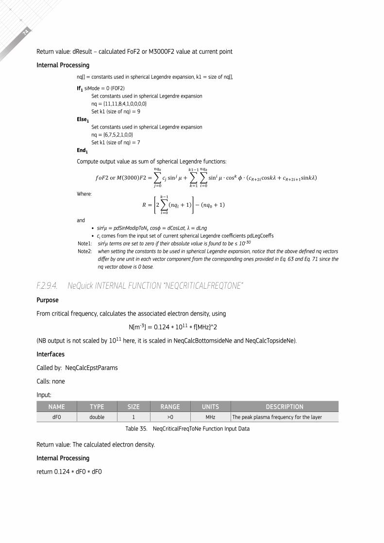
74

return value: dresult – calculated fof2 or m3000f2 value at current point

Internal Processing

nq[] = constants used in spherical legendre expansion, k1 = size of nq[],

If1 simode = 0 (f0f2)set constants used in spherical legendre expansion nq = {11,11,8,4,1,0,0,0,0}set k1 (size of nq) = 9

Else1set constants used in spherical legendre expansion nq = {6,7,5,2,1,0,0}set k1 (size of nq) = 7

End1

compute output value as sum of spherical legendre functions:

where:

and • siniμ = pdSinModipToNi, cosφ = dCosLat, λ = dLng • ci comes from the input set of current spherical legendre coefficients pdlegcoeffs

note1: siniμ terms are set to zero if their absolute value is found to be ≤ 10-30

note2: when setting the constants to be used in spherical Legendre expansion, notice that the above defined nq vectors differ by one unit in each vector component from the corresponding ones provided in Eq. 63 and Eq. 71 since the nq vector above is 0 base.

f.2.9.4. NeQuick iNTerNal fuNcTiON “NeQcriTicalfreQTONe”Purpose

from critical frequency, calculates the associated electron density, using

n[m-3] = 0.124 * 1011 * f[mhz]^2

(nb output is not scaled by 1011 here, it is scaled in neqcalcbottomsidene and neqcalctopsidene).

Interfaces


calls: none

Input:

return value: the calculated electron density.

Internal Processing

return 0.124 * df0 * df0

𝑓𝑓𝑓𝑓𝑓𝑓2 or 𝑀𝑀(3000)𝑓𝑓2 = ∑ 𝑐𝑐𝑗𝑗 sin𝑗𝑗 𝜇𝜇 +𝑛𝑛𝑞𝑞0

𝑗𝑗=0∑ ∑ sin 𝑖𝑖 𝜇𝜇

𝑛𝑛𝑞𝑞𝑘𝑘

𝑖𝑖=0∙ cos 𝑘𝑘 𝜙𝜙 ∙ (𝑐𝑐𝑅𝑅+2𝑖𝑖cos𝑘𝑘𝑘𝑘 + 𝑐𝑐𝑅𝑅+2𝑖𝑖+1sin𝑘𝑘𝑘𝑘)

𝑘𝑘1−1

𝑘𝑘=1

𝑅𝑅 = [2∑(𝑛𝑛𝑛𝑛𝑙𝑙 + 1)𝑘𝑘−1

𝑙𝑙=0] − (𝑛𝑛𝑛𝑛0 + 1)

NAmE tyPE SIzE RANGE UNItS DESCRIPtIONdf0 double 1 >0 mhz the peak plasma frequency for the layer

table 35. neqcriticalfreqtone function Input Data

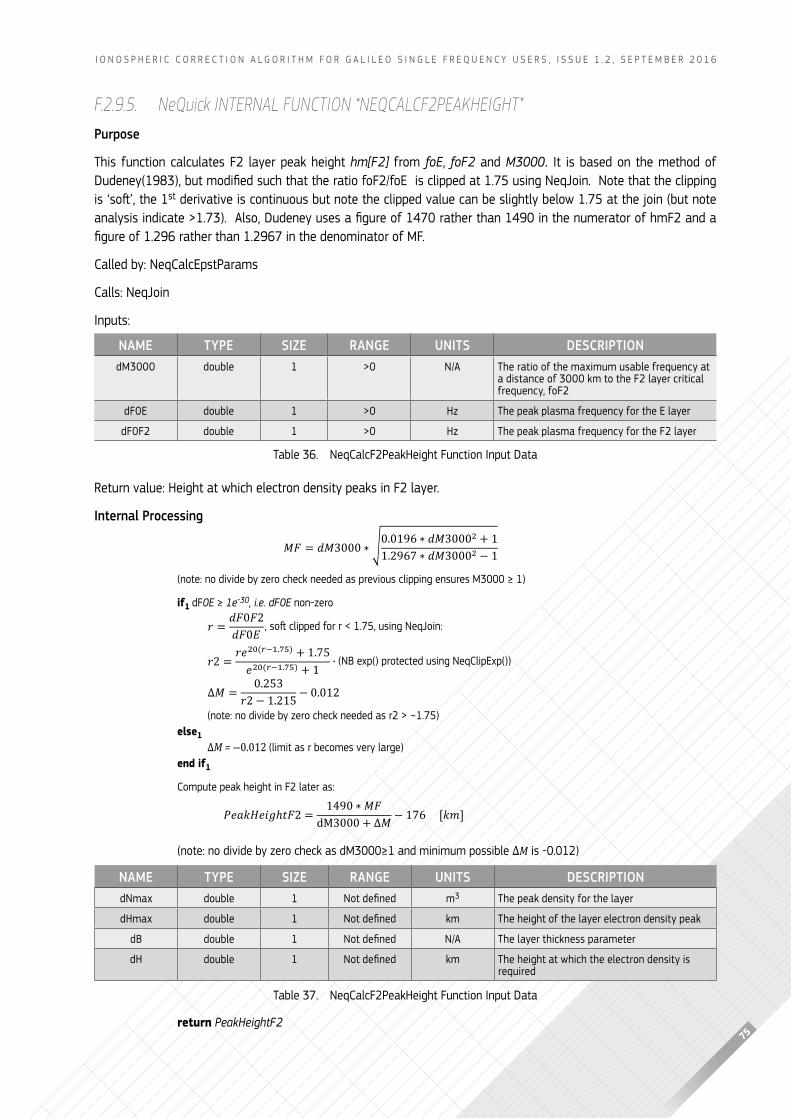
75


f.2.9.5. NeQuick iNTerNal fuNcTiON “NeQcalcf2PeakheiGhT”Purpose

this function calculates f2 layer peak height hm[F2] from foe, foF2 and M3000. It is based on the method of Dudeney(1983), but modified such that the ratio foF2/foE is clipped at 1.75 using neqJoin. note that the clipping is ‘soft’, the 1st derivative is continuous but note the clipped value can be slightly below 1.75 at the join (but note analysis indicate >1.73). also, Dudeney uses a figure of 1470 rather than 1490 in the numerator of hmF2 and a figure of 1.296 rather than 1.2967 in the denominator of mF.


calls: neqjoin

Inputs:

return value: height at which electron density peaks in f2 layer.

Internal Processing

(note: no divide by zero check needed as previous clipping ensures m3000 ≥ 1)

if1 df0e ≥ 1e-30, i�e� dF0e non-zero

𝑟𝑟 = 𝑑𝑑𝑑𝑑0𝑑𝑑2𝑑𝑑𝑑𝑑0𝐸𝐸 , soft clipped for r < 1.75, using neqJoin:

𝑟𝑟2 = 𝑟𝑟𝑟𝑟20(𝑟𝑟−1.75) + 1.75𝑟𝑟20(𝑟𝑟−1.75) + 1 ∙ (nb exp() protected using neqclipexp())

∆𝑀𝑀 = 0.253𝑟𝑟2 − 1.215 − 0.012

(note: no divide by zero check needed as r2 > ~1.75)else1

∆M = ―0.012 (limit as r becomes very large)end if1

compute peak height in f2 later as:

(note: no divide by zero check as dm3000≥1 and minimum possible ∆M is -0.012)

return PeakHeightF2

NAmE tyPE SIzE RANGE UNItS DESCRIPtIONdm3000 double 1 >0 n/A the ratio of the maximum usable frequency at

a distance of 3000 km to the f2 layer critical frequency, fof2

df0e double 1 >0 hz the peak plasma frequency for the e layer

df0f2 double 1 >0 hz the peak plasma frequency for the f2 layer

table 36. neqcalcf2peakheight function Input Data

𝑀𝑀𝑀𝑀 = 𝑑𝑑𝑀𝑀3000 ∗ √0.0196 ∗ 𝑑𝑑𝑀𝑀30002 + 1

1.2967 ∗ 𝑑𝑑𝑀𝑀30002 − 1

𝑃𝑃𝑃𝑃𝑃𝑃𝑃𝑃𝑃𝑃𝑃𝑃𝑃𝑃𝑃𝑃ℎ𝑡𝑡𝑡𝑡2 = 1490 ∗ 𝑀𝑀𝑡𝑡dM3000 + Δ𝑀𝑀 − 176 [𝑃𝑃𝑘𝑘]

NAmE tyPE SIzE RANGE UNItS DESCRIPtIONdnmax double 1 not defined m3 the peak density for the layer

dhmax double 1 not defined km the height of the layer electron density peak

db double 1 not defined n/A the layer thickness parameter

dh double 1 not defined km the height at which the electron density is required

table 37. neqcalcf2peakheight function Input Data

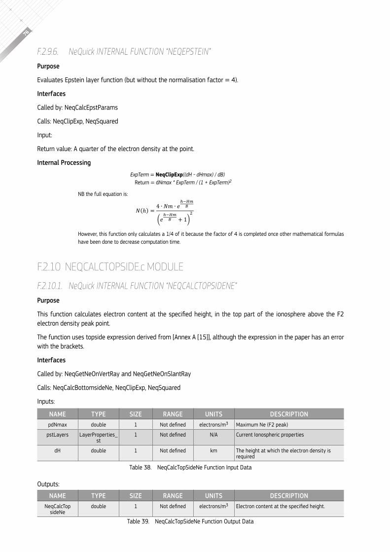
76

f.2.9.6. NeQuick iNTerNal fuNcTiON “NeQePsTeiN”Purpose

evaluates epstein layer function (but without the normalisation factor = 4).

Interfaces


calls: neqclipexp, neqsquared

Input:

return value: A quarter of the electron density at the point.

Internal Processing

ExpTerm = NeqClipExp((dH - dHmax) / dB)return = dNmax * ExpTerm / (1 + ExpTerm)2

nb the full equation is:

however, this function only calculates a 1/4 of it because the factor of 4 is completed once other mathematical formulas have been done to decrease computation time.

f.2.10 neqcalctopSide.c MODULE

f.2.10.1. NeQuick iNTerNal fuNcTiON “NeQcalcTOPsiDeNe”Purpose

This function calculates electron content at the specified height, in the top part of the ionosphere above the F2 electron density peak point.

the function uses topside expression derived from [Annex A [15]], although the expression in the paper has an error with the brackets.

Interfaces

called by: neqGetneonvertray and neqGetneonSlantray

calls: neqcalcbottomsidene, neqclipexp, neqsquared

Inputs:

outputs:

𝑁𝑁(ℎ) = 4 ∙ 𝑁𝑁𝑁𝑁 ∙ 𝑒𝑒ℎ−𝐻𝐻𝐻𝐻𝐵𝐵

(𝑒𝑒ℎ−𝐻𝐻𝐻𝐻𝐵𝐵 + 1)

2




dh double 1 not defined km the height at which the electron density is required

table 38. neqcalctopsidene function Input Data

NAmE tyPE SIzE RANGE UNItS DESCRIPtIONneqcalctop

sidenedouble 1 not defined electrons/m3 Electron content at the specified height.

table 39. neqcalctopsidene function output Data

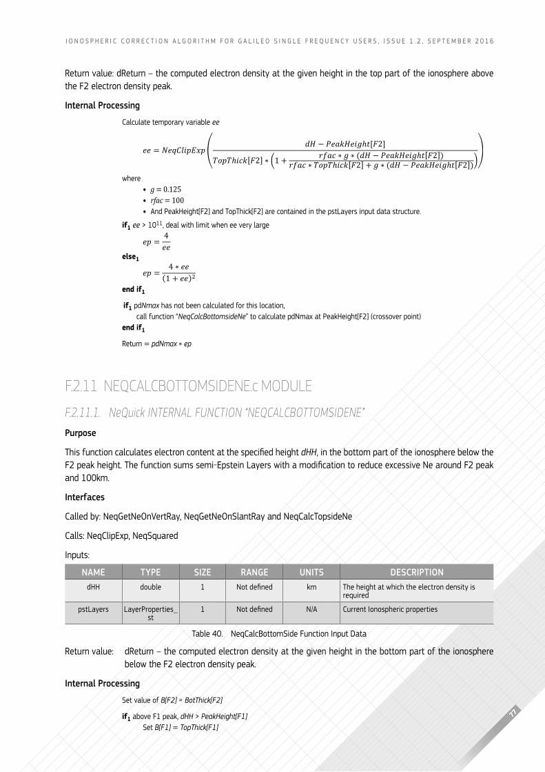
77


return value: dreturn – the computed electron density at the given height in the top part of the ionosphere above the f2 electron density peak.

Internal Processing

calculate temporary variable ee

𝑒𝑒𝑒𝑒 = 𝑁𝑁𝑒𝑒𝑁𝑁𝑁𝑁𝑁𝑁𝑁𝑁𝑁𝑁𝑁𝑁𝑁𝑁𝑁𝑁( 𝑑𝑑𝑑𝑑 − 𝑃𝑃𝑒𝑒𝑃𝑃𝑃𝑃𝑑𝑑𝑒𝑒𝑁𝑁𝑃𝑃ℎ𝑡𝑡[𝐹𝐹2]

𝑇𝑇𝑇𝑇𝑁𝑁𝑇𝑇ℎ𝑁𝑁𝑖𝑖𝑃𝑃[𝐹𝐹2] ∗ (1 + 𝑟𝑟𝑟𝑟𝑃𝑃𝑖𝑖 ∗ 𝑃𝑃 ∗ (𝑑𝑑𝑑𝑑 − 𝑃𝑃𝑒𝑒𝑃𝑃𝑃𝑃𝑑𝑑𝑒𝑒𝑁𝑁𝑃𝑃ℎ𝑡𝑡[𝐹𝐹2])𝑟𝑟𝑟𝑟𝑃𝑃𝑖𝑖 ∗ 𝑇𝑇𝑇𝑇𝑁𝑁𝑇𝑇ℎ𝑁𝑁𝑖𝑖𝑃𝑃[𝐹𝐹2] + 𝑃𝑃 ∗ (𝑑𝑑𝑑𝑑 − 𝑃𝑃𝑒𝑒𝑃𝑃𝑃𝑃𝑑𝑑𝑒𝑒𝑁𝑁𝑃𝑃ℎ𝑡𝑡[𝐹𝐹2]))

)

where • g = 0.125 • rfac = 100 • And peakheight[f2] and topthick[f2] are contained in the pstlayers input data structure.

if1 ee > 1011, deal with limit when ee very large

𝑒𝑒𝑒𝑒 = 4𝑒𝑒𝑒𝑒

else1

𝑒𝑒𝑒𝑒 = 4 ∗ 𝑒𝑒𝑒𝑒(1 + 𝑒𝑒𝑒𝑒)2

end if1

if1 pdNmax has not been calculated for this location, call function “NeqCalcBottomsideNe” to calculate pdnmax at peakheight[f2] (crossover point) end if1

return = pdNmax * ep

F.2.11 neqcalcbottomSidene.c MODULE

f.2.11.1. NeQuick iNTerNal fuNcTiON “NeQcalcBOTTOMsiDeNe”Purpose

This function calculates electron content at the specified height dHH, in the bottom part of the ionosphere below the F2 peak height. The function sums semi-Epstein layers with a modification to reduce excessive ne around F2 peak and 100km.

Interfaces

called by: neqGetneonvertray, neqGetneonSlantray and neqcalcTopsidene

calls: neqclipexp, neqsquared

Inputs:

return value: dreturn – the computed electron density at the given height in the bottom part of the ionosphere below the f2 electron density peak.

Internal Processing

set value of B[F2] = BotThick[F2]

if1 above f1 peak, dHH > PeakHeight[F1]set B[F1] = TopThick[F1]

NAmE tyPE SIzE RANGE UNItS DESCRIPtIONdhh double 1 not defined km the height at which the electron density is

required



table 40. neqcalcbottomside function Input Data

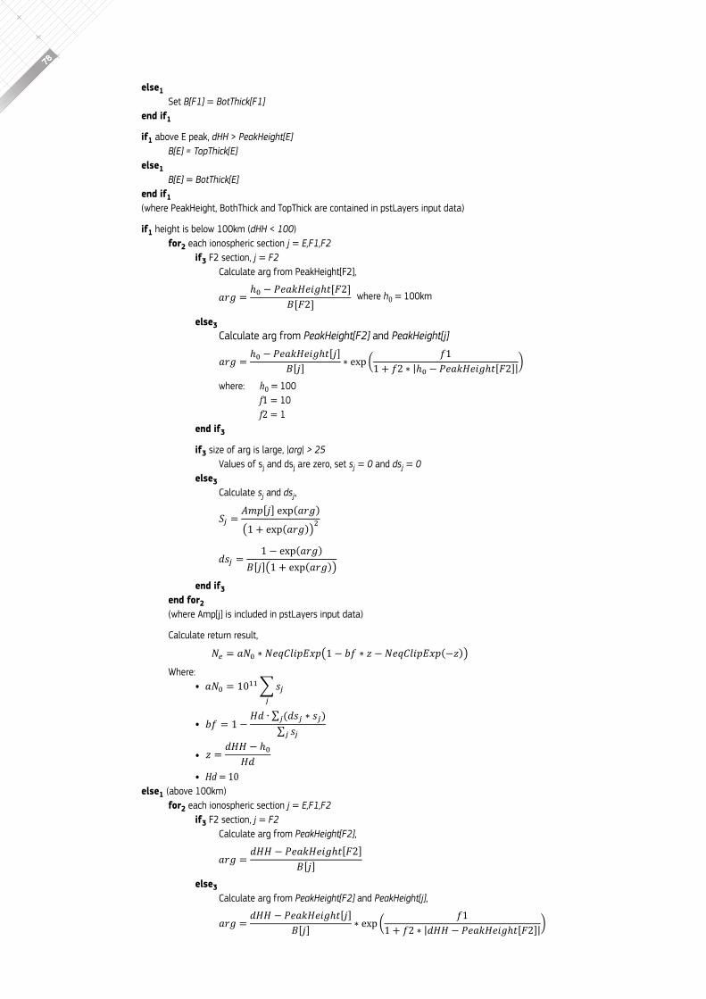
78

else1set B[F1] = BotThick[F1]

end if1

if1 above e peak, dHH > PeakHeight[e]B[E] = TopThick[E]

else1B[e] = BotThick[E]

end if1(where peakheight, boththick and topthick are contained in pstlayers input data)

if1 height is below 100km (dHH < 100)for2 each ionospheric section j = e,F1,F2

if3 f2 section, j = F2calculate arg from peakheight[f2],

𝑎𝑎𝑎𝑎𝑎𝑎 = ℎ0 − 𝑃𝑃𝑃𝑃𝑎𝑎𝑃𝑃𝑃𝑃𝑃𝑃𝑃𝑃𝑎𝑎ℎ𝑡𝑡[𝐹𝐹2]𝐵𝐵[𝐹𝐹2] where h0 = 100km

else3calculate arg from PeakHeight[F2] and PeakHeight[j]

𝑎𝑎𝑎𝑎𝑎𝑎 =ℎ0 − 𝑃𝑃𝑃𝑃𝑎𝑎𝑃𝑃𝑃𝑃𝑃𝑃𝑃𝑃𝑎𝑎ℎ𝑡𝑡[𝑗𝑗]

𝐵𝐵[𝑗𝑗] ∗ exp �𝑓𝑓1

1 + 𝑓𝑓2 ∗ |ℎ0 − 𝑃𝑃𝑃𝑃𝑎𝑎𝑃𝑃𝑃𝑃𝑃𝑃𝑃𝑃𝑎𝑎ℎ𝑡𝑡[𝐹𝐹2]|�

where: h0 = 100 f1 = 10 f2 = 1

end if3

if3 size of arg is large, |arg| > 25values of sj and dsj are zero, set sj = 0 and dsj = 0

else3calculate sj and dsj,

𝑆𝑆𝑗𝑗 = 𝐴𝐴𝐴𝐴𝐴𝐴[𝑗𝑗] exp(𝑎𝑎𝑎𝑎𝑎𝑎)(1 + exp(𝑎𝑎𝑎𝑎𝑎𝑎))2

𝑑𝑑𝑑𝑑𝑗𝑗 =1 − exp(𝑎𝑎𝑎𝑎𝑎𝑎)

𝐵𝐵[𝑗𝑗](1 + exp(𝑎𝑎𝑎𝑎𝑎𝑎))

end if3end for2(where Amp[j] is included in pstlayers input data)

calculate return result,

where: • 𝑎𝑎𝑁𝑁0 = 1011∑𝑠𝑠𝑗𝑗

𝑗𝑗

• 𝑏𝑏𝑏𝑏 = 1 −𝐻𝐻𝐻𝐻 ∙ ∑ (𝐻𝐻𝑑𝑑𝑗𝑗 ∗ 𝑑𝑑𝑗𝑗)𝑗𝑗

∑ 𝑑𝑑𝑗𝑗𝑗𝑗

• 𝑧𝑧 = 𝑑𝑑𝑑𝑑𝑑𝑑 − ℎ0𝑑𝑑𝑑𝑑

• Hd = 10else1 (above 100km)

for2 each ionospheric section j = e,F1,F2if3 f2 section, j = F2

calculate arg from PeakHeight[F2],

𝑎𝑎𝑎𝑎𝑎𝑎 = 𝑑𝑑𝑑𝑑𝑑𝑑 − 𝑃𝑃𝑃𝑃𝑎𝑎𝑃𝑃𝑑𝑑𝑃𝑃𝑃𝑃𝑎𝑎ℎ𝑡𝑡[𝐹𝐹2]𝐵𝐵[𝑗𝑗]

else3calculate arg from PeakHeight[F2] and PeakHeight[j],

𝑎𝑎𝑎𝑎𝑎𝑎 =𝑑𝑑𝑑𝑑𝑑𝑑 − 𝑃𝑃𝑃𝑃𝑎𝑎𝑃𝑃𝑑𝑑𝑃𝑃𝑃𝑃𝑎𝑎ℎ𝑡𝑡[𝑗𝑗]

𝐵𝐵[𝑗𝑗] ∗ exp �𝑓𝑓1

1 + 𝑓𝑓2 ∗ |𝑑𝑑𝑑𝑑𝑑𝑑 − 𝑃𝑃𝑃𝑃𝑎𝑎𝑃𝑃𝑑𝑑𝑃𝑃𝑃𝑃𝑎𝑎ℎ𝑡𝑡[𝐹𝐹2]|�

𝑁𝑁𝑒𝑒 = 𝑎𝑎𝑁𝑁0 ∗ 𝑁𝑁𝑁𝑁𝑁𝑁𝑁𝑁𝑁𝑁𝑁𝑁𝑁𝑁𝑁𝑁𝑁𝑁𝑁𝑁(1 − 𝑏𝑏𝑏𝑏 ∗ 𝑧𝑧 − 𝑁𝑁𝑁𝑁𝑁𝑁𝑁𝑁𝑁𝑁𝑁𝑁𝑁𝑁𝑁𝑁𝑁𝑁𝑁𝑁(−𝑧𝑧))

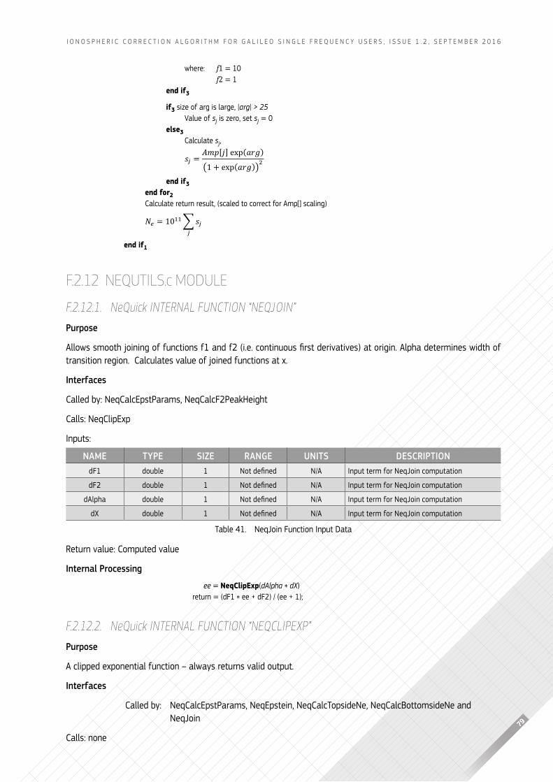
79


where: f1 = 10 f2 = 1

end if3

if3 size of arg is large, |arg| > 25value of sj is zero, set sj = 0

else3calculate sj,

𝑠𝑠𝑗𝑗 = 𝐴𝐴𝐴𝐴𝐴𝐴[𝑗𝑗] exp(𝑎𝑎𝑎𝑎𝑎𝑎)(1 + exp(𝑎𝑎𝑎𝑎𝑎𝑎))2

end if3end for2calculate return result, (scaled to correct for Amp[] scaling)

𝑁𝑁𝑒𝑒 = 1011∑𝑠𝑠𝑗𝑗𝑗𝑗

end if1

F.2.12 nequtilS.c MODULE

f.2.12.1. NeQuick iNTerNal fuNcTiON “NeQJOiN”Purpose

allows smooth joining of functions f1 and f2 (i.e. continuous first derivatives) at origin. alpha determines width of transition region. calculates value of joined functions at x.

Interfaces

called by: neqcalcepstparams, neqcalcf2peakheight

calls: neqclipexp

Inputs:

return value: computed value

Internal Processing

ee = NeqClipExp(dAlpha * dX)return = (df1 * ee + dF2) / (ee + 1);

f.2.12.2. NeQuick iNTerNal fuNcTiON “NeQcliPexP”Purpose

A clipped exponential function – always returns valid output.

Interfaces

called by: neqcalcepstparams, neqepstein, neqcalctopsidene, neqcalcbottomsidene and neqjoin

calls: none

NAmE tyPE SIzE RANGE UNItS DESCRIPtIONdf1 double 1 not defined n/A Input term for neqjoin computation

df2 double 1 not defined n/A Input term for neqjoin computation

dAlpha double 1 not defined n/A Input term for neqjoin computation

dx double 1 not defined n/A Input term for neqjoin computation

table 41. neqjoin function Input Data

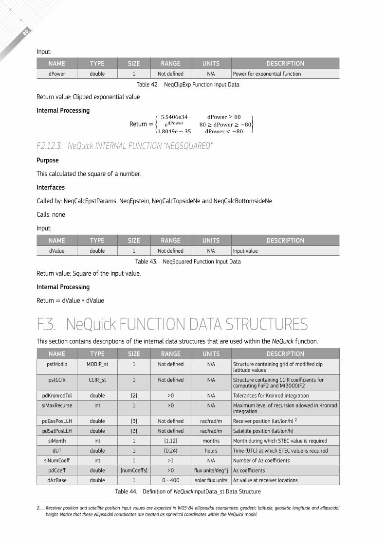
80

Input:

return value: clipped exponential value

Internal Processing

return =

f.2.12.3. NeQuick iNTerNal fuNcTiON “NeQsQuareD”Purpose

this calculated the square of a number.

Interfaces

called by: neqcalcepstparams, neqepstein, neqcalctopsidene and neqcalcbottomsidene

calls: none

Input:

return value: square of the input value.

Internal Processing

return = dvalue * dvalue

F.3. Nequick FUNCTION DATA STRUCTURESthis section contains descriptions of the internal data structures that are used within the NeQuick function.

NAmE tyPE SIzE RANGE UNItS DESCRIPtIONdpower double 1 not defined n/A power for exponential function

table 42. neqclipexp function Input Data

Return = �5.5406e34 dPower > 80

edPower 80 ≥ dPower ≥ −801.8049e− 35 dPower < −80

�

NAmE tyPE SIzE RANGE UNItS DESCRIPtIONdvalue double 1 not defined n/A Input value

table 43. neqsquared function Input Data

NAmE tyPE SIzE RANGE UNItS DESCRIPtIONpstmodip moDIp_st 1 not defined n/A Structure containing grid of modified dip

latitude values

pstccIr ccIr_st 1 not defined n/A Structure containing ccir coefficients for computing fof2 and m(3000)f2

pdkronrodtol double [2] >0 n/A tolerances for kronrod integration

simaxrecurse int 1 >0 n/A maximum level of recursion allowed in kronrod integration

pdgssposllh double [3] not defined rad/rad/m receiver position (lat/lon/h) 2

pdsatposllh double [3] not defined rad/rad/m satellite position (lat/lon/h)

simonth int 1 [1,12] months month during which stec value is required

dut double 1 [0,24) hours time (utc) at which stec value is required

sinumcoeff int 1 ≥1 n/A number of az coefficients

pdcoeff double [numcoeffs] >0 flux units/deg^j az coefficients

dAzbase double 1 0 - 400 solar flux units Az value at receiver locations

2 ��Receiver position and satellite position input values are expected in WGS-84 ellipsoidal coordinates: geodetic latitude, geodetic longitude and ellipsoidal height. Notice that these ellipsoidal coordinates are treated as spherical coordinates within the NeQuick model.

table 44. Definition of NeQuickInputData_st Data structure

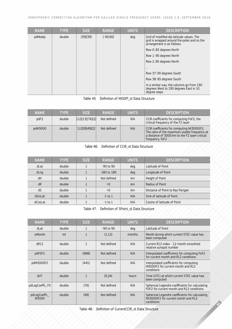
81


NAmE tyPE SIzE RANGE UNItS DESCRIPtIONpdmodip double [39][39] [-90,90] deg Grid of modified dip latitude values. The

grid is wrapped around the poles and so the arrangement is as follows:

row 0: 85 degrees north



…

row 37: 90 degrees south

row 38: 85 degrees south

In a similar way, the columns go from 190 degrees west to 190 degrees east in 10 degree steps

table 45. Definition of MODiP_st Data structure

NAmE tyPE SIzE RANGE UNItS DESCRIPtIONpdf2 double [12][13][76][2] not defined n/A ccir coefficients for computing FoF2, the

critical frequency of the f2 layer

pdm3000 double [12][9][49][2] not defined n/A ccir coefficients for computing m(3000)F2, the ratio of the maximum usable frequency at a distance of 3000 km to the f2 layer critical frequency, fof2

table 46. Definition of ccir_st Data Structure


dlng double 1 -180 to 180 deg longitude of point

dh double 1 not defined km height of point

dr double 1 >0 km radius of point

ds double 1 >0 km Distance of point to ray parigee

dsinlat double 1 -1 to 1 n/A sine of latitude of point

dcoslat double 1 -1 to 1 n/A cosine of latitude of point

table 47. Definition of Spoint_st Data Structure


simonth int 1 [1,12] months month during which current stec value has been computed

dr12 double 1 not defined n/A current r12 index - 12-month smoothed relative sunspot number

pdf0f2 double [988] not defined n/A interpolated coefficients for computing FoF2 for current month and r12 conditions

pdm3000f2 double [441] not defined n/A interpolated coefficients for computing m3000f2 for current month and r12 conditions

dut double 1 [0,24) hours time (utc) at which current stec value has been computed

pdlegcoeffs_F0 double [76] not defined n/A Spherical legendre coefficients for calculating f0f2 for current month and r12 conditions

pdlegcoeffs_m3000

double [49] not defined n/A Spherical legendre coefficients for calculating m(3000)f2 for current month and r12 conditions

table 48. Definition of currentccir_st Data Structure

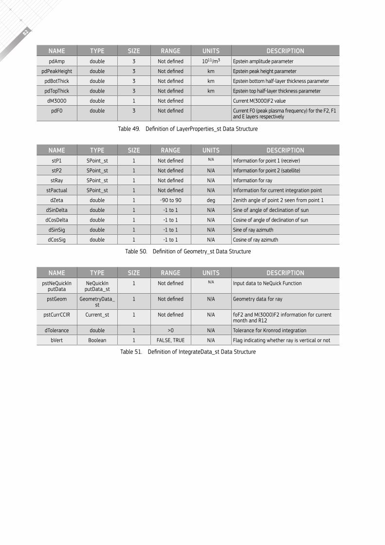
82

NAmE tyPE SIzE RANGE UNItS DESCRIPtIONpdAmp double 3 not defined 1011/m3 epstein amplitude parameter

pdpeakheight double 3 not defined km epstein peak height parameter

pdbotthick double 3 not defined km epstein bottom half-layer thickness parameter

pdtopthick double 3 not defined km epstein top half-layer thickness parameter

dm3000 double 1 not defined current m(3000)f2 value

pdf0 double 3 not defined current f0 (peak plasma frequency) for the f2, f1 and e layers respectively

table 49. Definition of layerproperties_st Data Structure

NAmE tyPE SIzE RANGE UNItS DESCRIPtIONstp1 spoint_st 1 not defined n/A Information for point 1 (receiver)

stp2 spoint_st 1 not defined n/A Information for point 2 (satellite)

stray spoint_st 1 not defined n/A Information for ray

stpactual spoint_st 1 not defined n/A Information for current integration point

dzeta double 1 -90 to 90 deg zenith angle of point 2 seen from point 1

dsinDelta double 1 -1 to 1 n/A sine of angle of declination of sun

dcosDelta double 1 -1 to 1 n/A cosine of angle of declination of sun

dsinsig double 1 -1 to 1 n/A sine of ray azimuth

dcossig double 1 -1 to 1 n/A cosine of ray azimuth

table 50. Definition of Geometry_st Data Structure

NAmE tyPE SIzE RANGE UNItS DESCRIPtIONpstnequickIn

putDatanequickIn putData_st

1 not defined n/A Input data to nequick function

pstgeom geometryData_st

1 not defined n/A geometry data for ray

pstcurrccIr current_st 1 not defined n/A fof2 and m(3000)f2 information for current month and r12

dtolerance double 1 >0 n/A tolerance for kronrod integration

bvert boolean 1 fAlse, true n/A flag indicating whether ray is vertical or not

table 51. Definition of integrateData_st Data Structure

83


Documents

Ionospheric Correction Algorithm for Galileo Single ... · iii ionospheric correction algorithm for galileo single freuenc users, issue 1.2, september 2016 table of contents section