1

Ionospheric Electron Density Profiles Obtained

With the Global Positioning System: Results From

the GPMMET Experiment

George Hajj and Larry Remans

Jet Propulsion Laboratory, California Institute of Technology

2

ABSTRACT

The GPS/MET experiment, which placed a GPS receiver in a low-Earth orbit tracking GPS

satellites setting behind the Earth’s limb, has collected data from several thousands of

occultations since its launch in April 1995. This experiment demonstrated for the first time

the use of GPS in obtaining profiles of electron density and other geophysical variables

such as temperature, pressure and water vapor in the lower atmosphere. This paper

presents a set of ionospheric profiles obtained from GPWMET with the Abel inversion

technique. The effects of the ionosphere on the GPS signal during occultation, such as

bending and scintillation, are examined. Electron density profiles are obtained using the

Abel inversion technique and compared to ones obtained from the Parametrized Ionospheric

Model (PIM) and to ionosonde and incoherent scatter radar measurements. Statistical

comparisons of N~F2 values obtained from GPSM4ET and ionosondes indicate that these

two types of measurements agree to -20% (1 sigma).

.

3

1. INTRODUCTION

In April, 1995, the GPS/MET (for GPS Meteorology) experiment placed a GPS receiver in

a low-Earth orbit (LEO) tracking the global positioning system (GPS) satellites as they set

behind the Earth’s atmosphere. The basic concept of the GPS radio occultation technique

is a simple one. When a signal transmitted by a GPS satellite and received by a LEO

satellite passes through the Earth’s atmosphere in a limb sounding geometry [Fig. 1], its

phase and amplitude are affected in ways that are characteristic of the index of refraction of

the medium along the path of propagation. By applying certain assumptions on the

variability of the index of refraction of the propagating media (e.g. spherical symmetry in

the locality of the occultation), phase change measurements between the transmitter and the

receiver yield refractivity profiles in the ionosphere (-60-1000 km) and lower neutral

atmosphere (0-60 km). The refractivity, in turn, yields electron density in the ionosphere,

temperature and pressure in the neutral stratosphere and upper troposphere, and (with the

aid of independent temperature data) water vapor density in the lower troposphere.

This method has been applied repeatedly in NASA’s planetary occultation

experiments [see e.g. Fjeldbo, 1971 and Tyler, 1987] and was inherited from the area of

geological mapping of the Earth’s interior. However, the application of the technique to

sense the Earth’s neutral atmosphere or ionosphere had to await the development of an

infrastructure built for completely different purposes, namely, the set of 24 GPS satellites

launched and maintained by the Department of Defense for the purpose of navigation.

Once this set of satellites became operational, it became clear to some (e.g. Gurvich and

Kasil’nikova [1987], Yunck et al. [1988]) that placing one receiver in LEO, with a full

360° field of view of the Earth’s limb, will provide about 500 globally distributed

occultations daily at a very low cost. This concept was tested for the first time with the

GPS/MET experiment, managed by the University Corporation for Atmospheric Research

(UCAR) [Ware et al., 1996], consisting of a 2 kg GPS receiver piggybacked on the

4

MicroLab I satellite having a circular orbit of 740 km altitude and 70° inclination. The

GPS receiver is a space qualified TurboRogue [Meehan et al., 1992] capable of tracking up

to 8 GPS satellites simultaneously at both frequencies transmitted by GPS. Due to the

limited field of view of the GPS receiver’s antenna and the onboard memory of the satellite,

the GPWMET collects anywhere between 100-200 globally distributed occultations daily.

Since the start of the GPSIMET experiment in April of 1995, tens of thousands of

occultations have been recorded by GPSIMET, providing a very rich data set to study the

ionosphere and the lower neutral atmosphere.

Due to the abundance of neutral atmospheric data from radiosondes and the

existence of accurate numerical weather models, several studies that examine the accuracies

of temperature and pressure profiles obtain from GPSIMET have been published. For

example, Kursinski et al. (1996) and Ware et al. (1996) demonstrated that GPS/MET

temperature profiles are accurate to better than 1-2 K between -5-30 altitudes, while Leroy

(1997) showed that geopotential heights of pressure levels in the same region are accurate

to better than 20 meters. In the ionosphere, on the other hand, due to the sparsity of data,

comparisons have been somewhat limited. In order to assess the accuracy of ionospheric

electron densities derived from GPS occultations, several investigators have performed

simulated experiments where synthetic data based on ionospheric models have been created

and then inverted (see e.g. Hajj et al., 1994; H@eg et al., 1995; Decker et al., 1996;

Leitinger et al. 1997). Those studies suggested several possible ways of inverting TEC

data obtained from GPS occultations starting from the simplest approach of assuming a

spherically symmetric medium and solving for an electron density profile for each

occultation (e.g. Abel inversion approach presented below), to combining different

occultations along with ground data to obtain 2-D or 3-D images of the ionosphere

(tomographic inversions). While it is obvious that the assumption of spherical symmetry in

the ionosphere is never an accurate one, the Abel inversion approach serves well as a

starting point to understand some of the unique features associated with GPS occultation

5

data. The purpose of this paper is to examine some of these features and to estimate the

accuracy of retrieved electron density profiles obtained with the Abel inversion by

comparing to other independent measurements such as incoherent scatter radar and

ionosondes. The accuracy obtained with this approach will be a lower bound on what can

be achieved with more elaborate inversion methods.

The outline of the paper is as follows. Section two will briefly explain the Abel

inversion technique as applicable to the ionosphere. Section three will examine some of the

effects of the ionosphere on occulting signals, including bending and scintillation. Section

four will present some results of electron density profiles, the coverage obtained with

GPWMET, and some comparisons to ionospheric models and to ionospheric measurements

from incoherent scatter radars and ionosondes. Some conclusions are discussed in section

five.

2. RADIO OCCULTATION TECHNIQUE—THE ABEL INVERSION

The basic observable for each occultation is the phase change between the transmitter and

the receiver as the signal propagates through the ionosphere and the neutral atmosphere

[Fig. 1]. A GPS phase measurement can be modeled as

@ = p + B“”’” - B’”+ An’Utr”l + Ai”n” + b (1)

where p is the geometrical range, Bfr”n’ and B’” are clock biases for the transmitter and the

receiver, respectively, fl’”’r”~ and d“””” are the delays due to the neutral atmosphere and the

ionosphere, and b is a phase ambiguity. In addition to the occulting GPS and LEO

satellites, other measurements, taken from a network of ground receivers tracking GPS and

from the LEO tracking other GPS satellites, are used to obtain precise orbit and clock

6

solutions of the satellites. The details of how the GPS/MET signal is calibrated in order to

isolate the atmospheric effects on the occulting signals are given elsewhere [Hajj et al.,

1995]. Here it suffices to say that through the calibration process the sum of the neutral

and the ionospheric delays is isolated (up to a constant). For the occulting link going

through the ionosphere, the neutral delay is negligible. This extra phase change induced by

the medium is then differentiated (after proper smoothing) to obtain the extra Doppler shift

induced by the medium. This extra Doppler shift can be used to derive the bending of the

signal, et, as a function of the asymptote miss distance, a, [Fig. 1] by assuming a

spherically symmetric atmosphere in the locality of the occultation; the relationship between

the direction of the signal’s propagation and the extra Doppler shift, Af, is then given by

(2)

where~is the operating frequency, c is the speed of light, ~, and;, are the transmitter and

receiver velocity respectively, ~, and ~, are the unit vectors in the direction of the

transmitted and received signal respectively, and ~ is the unit vector in the direction of the

straight line connecting the transmitter to the receiver. Assuming spherical symmetry

introduces the extra constraint

(3)

where ?, and ?, are the coordinates of the transmitter and the receiver respectively, and n

is the index of refraction at the specified coordinate. Eqs. (2) and (3) can be solved

simultaneously in order to estimate the total atmospheric bending. Solving these two

equations ideally requires knowledge of n at the satellites locations; however, in an

appendix we estimate that by setting n= 1 at the transmitter or the receiver (when

receiver is at reasonably high altitude, such as the case for the GPWMET experiment),

7

the

the

solved-for ionospheric bending and the corresponding electron density are overestimated

by no more than 0.5% of their true values. We proceed therefore by setting

n(~) =n(fr)=l.

The spherical symmetry assumption can also be used to relate the signal’s bending

to the medium’s index of refraction, n, via the relation [Born and Wolf, 1980, page 123]:

.

J

din(n) da,a(a) = –2a

~~ da’ ,a (4)

where a = w and r is the radius of the tangent point [Fig. 1]. This integral equation can

then be inverted by using an Abel integral transform given by [see e.g. Tricomi, 1985,

page 39]

ln(n(a)) = –1J- a(a’ ) da!

~am . (5a)

The upper limit of the integral in Eq. (5) requires knowledge of the bending as a function of

a all the way up to the top of the ionosphere. The GPS is above most of the ionosphere;

however, this is not true of the GPS/MET instrument,at7110 km radius (740 km altitude).

In order to obtain u(a) for a > 7110, an exponential extrapolation a(a) based on

information from a c 7110 is used. In order to avoid dealing with the singularity at the

lower bowndary of the integral, Eq. (5a) is rewritten as

8

[

In(n(a)) = –~ a(ain,)ln(ain, + ~~) – cx(a)ln(a) – ~ln(a’+-)d~$)daa 1

1

J

cx(a’ ) da,——?ra,Jm-

,“

(5.b)where ai~, is an intermediate value between a and co and is normally chosen to be slightly

larger than a. The terms in bracket on the right hand side of Eq. (5.b) are the result of

integration by parts.

In the ionosphere, the index of refraction is related to electron density via

n = 1 -40.3x~f2(6)

where n, is the electron density in m-q and~ is the operating frequency in Hz. Eqs. (2)-(6)

constitute the essence of the radio occultation profiling technique as it applies to the

ionosphere. In the next two sections we will examine bending and electron density profiles

derived with this technique.

3. I O N O S P H E R I C B E N D I N G A N D S C I N T I L L A T I O N O F G P S

OCCULTING SIGNALS

Data examined in this section were taken on May 4-5, 1995. During this period (and for

much of the GPS/MET experiment) the L1 and L2 phase measurements for the occulting

link were recorded once every 10 seconds when the tangent point was above -120 km

altitude, and once every 20 msec (50 Hz rate) when the tangent point was below that

height. This is because the GPS/MET experiment’s primary goal is to sense the lower

neutral atmosphere. Therefore, results presented in this and the next section will reflect a

9

rather coarse vertical resolution (-20-30 km) above -120 km and a much finer vertical

resolution (of order 1,5 km, corresponding to l/2-second smoothing in the processing)

below -120 km altitude.

Based on Snell’s law, the bending of the signal locally is in the direction of the

refractivity gradient, In a general and approximate sense, the gradient of refractivity in the

ionosphere is pointing upward above the F2 peak and downward below that peak.

Therefore, the GPS signals will generally bend upward and downward above and below

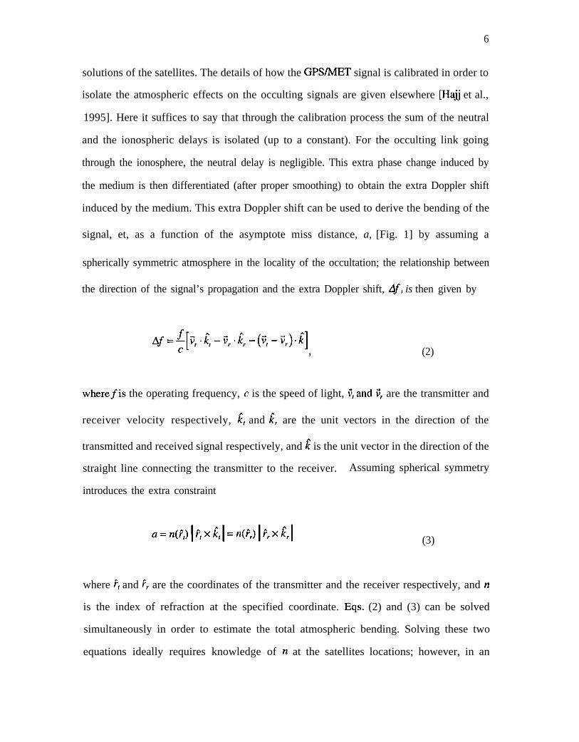
the F2 peak respectively. Examining the bending of the GPS L1 signal for 61 GPS/MET

occultations that took place on May 4, 1995, we observe the following features [Fig. 2]:

1-The bending varies about two orders of magnitude between 0.0001-0.01 degrees (cannot

be seen from the scale of Fig. 2) depending on local time and geographical location of the

occultation. Since 1995 falls near a solar-minimum condition, the largest bending of figure

2 can be an order of magnitude smaller than the corresponding solar-maximum condition,

2-The highest peak in bending, which is associated with the F2 peak, varies in height

between -250-400 km, consistent with F2 peak heights at different

times.

3-With negative bending defined to be toward the earth, the signal

latitudes and local

bends away from

(toward) the Earth above (below) well defined peaks in the ionosphere such as the F2 and

the E peaks. Since the bending of the signal depends on the gradient of the refractivity

(which is vertical, to first order), one expects to see a change of sign in the bending as the

tangent point samples through a peak.

4-Very sharp variations of bending are associated with sporadic E layers. The largest

absolute bending for this particular day is -0.03 degrees, which corresponds to the signal

just descending below a sporadic E-layer. The fact that the bending induced by the

sporadic E is larger than that of the F2 is due to the very short scale height associated with

the sporadic E-layer, which makes the refractivity gradient largest there.

5-The tails at the bottom end of all these curves start to grow in magnitude due to the

neutral atmospheric bending which dominates below about 50 km altitude.

The most striking feature of these data is how sharp the signature is around the E-

(or sporadic E-) layer. Even though determination of the magnitude of the E-peak electron

density might be obscured due to the overlaying layers and the assumption of spherical

symmetry, the height of sharp E-layer appears to be reasonably well determined.

However, no strong conclusion can be drawn on the accuracy of these heights without

further analysis and simulation accounting for the E-layer variability being frequently quite

regional and the effect of spherical symmetry assumption on the retrieval.

Bending for the L2 signal is a factor of 1.65 (= (154/120)2, the square of the ratio

of L1 to L2 frequencies) larger than for L1 (see Eq. (6)). This dispersive nature of the

ionosphere causes the L1 and L2 signals to travel slightly different paths and therefore

sample different regions (as indicated by the solid and dashed lines in Fig. 1). This causes

the tangent points of the two links to be at different heights in the atmosphere at a specific

time. With the Abel inversion technique, the electron density profile and the height of the

tangent point at a particular instant during the occultation can be solved for. Fig. 3 shows

an example of an electron density retrievaJ obtained from GPWMET for an occultation

taking place near -6N latitude and 228E longitude around 20:04 UT of May 4, 1995 (the

corresponding local time is 11:01). Also shown on the figure is the separation between the

L1 and L2 tangent points as a function of altitude. In the neighborhood of the F2 peak, the

relative position of the two signals change due to changing direction of bending. Above the

F2 peak, since the bending is generally upward, the L2 tangent point will always be lower

than the L1 tangent point The situation reverses when the signal tangent point is below the

F2 peak. For this particular profile, the maximum separation is of order 300 meters; this

scales linearly with the amount of bending a signal experiences. Therefore, one can expect

separations that are two orders of magnitude smaller (as seen with the bending) or one

order of magnitude larger during solar-max day-time. A large separation of the two signals

can be a limiting error for neutral atmospheric retrievals at altitudes above -40 km

[Kursinski et al., 1997] unless higher order corrections are applied to calibrate for the

ionosphere.

We now turn our attention to some amplitude data obtained from GPWMET. Fig. 4

shows the flight receiver signal-to-noise ratio of the L1 and L2 signals for four different

occultations, where time = O corresponds to the start of high-rate data at about 120 km

altitude for each occultation. The gradual decrease of SNR starting at about 30-40 seconds

is due to significant atmospheric bending starting at about the tropopause. As the signal

approaches the surface, it bends significantly (up to - 10), defocuses and finally disappears.

Nearly half of the occultation displays a smooth steady SNR while the signal is in the

ionosphere. Figure 4.d is an example of such smooth SNR. However, a good fraction of

them (see Fig. 4a, b and c) show one or several sharp changes in SNR which can be

attributed to sharp layers (e.g. sporadic E) at the bottom of the ionosphere. That these

scintillations are caused by the ionosphere and not the neutral atmosphere can be seen from

the fact that the L2 SNR fluctuation is larger than that of L 1, consistent with its lower

carrier frequency.

The electron density profiles obtained with the Abel inversion corresponding to the

occultations of Fig. 4 are shown in Fig. 5. Fig. 5a, b and c respectively show one,

several and two sharp layers at the bottom of the ionosphere.

4. OCCULTATION COVERAGE AND ELECTRON DENSITY PROFILING

As mentioned above, due to the antenna field-of-view (*30”) and memory limitations on

board the satellite, only 100-200 occultations per day are collected from the GPWMET.

The coverage obtained during 20 days of the mission (April 24 and 25, May 3 and 4, June

21-24 and 27-30, July 1-7 of 1995) is shown in Fig. 6a, where each occultation is

represented by one point (average location of geographic latitude and longitude of the

occultation tangent point). By contrast, the GPS/MET coverage for one day in sun-fixed

coordinate is shown in Fig. 6.b where each line corresponds to one occultation intersecting

the ionospheric shell between 100-400 km altitude.

Since the coverage In Fig. 6.b is shown as a function of sun-fixed longitude (O

sun-fixed longitude corresponds to noon local time), and the occultations are scattered

along the LEO orbit, the occultations are concentrated along the ground track of the

GPWMET satellite. At mid- and low-latitude the LEO samples the ionosphere at about the

same latitude and local time for every revolution of the LEO orbit, This local time will

precess slowly with the precession of the LEO orbit. For GPSIMET, it takes 110 days for

a full precession of the satellite; therefore, it takes half of this period to sample the Earth at

all local times for mid- and low-latitude. On the other hand, at high latitude, the same 12

hour period is sampled for a given hemisphere (e.g. in Fig. 6.b the northern hemisphere is

always sampled between noon and midnight local time whereas the southern hemisphere is

sampled between midnight and noon local time). It takes half of the precession period to

reverse the sampling geomet~.

The width of the spread of occultations around the LEO track is determined by the

width of the field-of-view of the receiving antenna and the distance to the limb. For a 740

km altitude satellite (such as GPWMET) the limb is about 3000 km away from the satellite.

This implies that the tangent point of an occultation falls within a 3000 km radius from the

satellite trajectory during that occultation, setting an upper limit on the width of the spread

of occultations around the LEO track to be -*27 equatorial degrees.

The reoccurrence of occultations at nearby local times and latitudes is illustrated by

showing the retrievals of four equatorial occultations appearing at consecutive orbital

revolutions, each taking place near noon local time. (These four occultations cross the

circle in the middle of Fig. 6. b.) The electron density retrievals for these four occultations

(using the Abel inversion) are shown in Fig. 7a.

13

For comparisons, profiles obtained from the Ionospheric Parametrized Model

(PIM) [Daniell et al., 1995] derived with input parameters suitable for the same day are also

shown. Some of the main features to observe are: (1) the ability to observe the E-, F1 - and

F2-layers that are characteristic of mid- and low-latitude day-time ionosphere. (2) The

ability to observe the evolution of the ionosphere at the same local time and latitude every

-100 minutes (the GPWMET orbital period) for mid- and low-latitude occultations. (3)

Except for the far-left profile shown in 7a, the PIM reproduces F2 peak densities and

heights that are in reasonable agreement with the GPS/MET retrieval. (4) Comparisons

with the PIM is generally better below the F2-peak than at the top-side. (5) The ability of

both the model and the retrievals to reproduce the sharp bottom of the ionosphere. Other

examples of GPS/MET retrieved profiles are shown for high latitude between dusk and

midnight local time in Fig. 7.b. We note the low F2-peak height, the near disappearance of

the F1-peak, and the very low peak density near midnight local time (far-right in Fig. 7 b).

In contrast to the equatorial profiles the comparison with the PIM model appears to be more

favorable at the top-side than below the F2-peak,

Comparisons of GPSLMETprofiles to ISR and ionosonde

In order to assess the accuracy of the GPSIMET retrievals, coincidences of other

types of data such as ionosondes or incoherent scatter radar (ISR) with GPSIMET

occultations have been examined, Fig. 8 .a shows a GPS/MET profile obtain on May 5,

1995, at about 0320 UT, with tangent points coordinates about 41 .9N and 282.3E (the

tangent points for this occultation drifted between 40-43.8N and 281. 1-283.6E during the

4 minutes of the occultation). On the same figure are two ISR measurements of electron

density obtained with a 640 microsecond pulse mode at about the same time and 20 minutes

after the occultation. In Fig. 8.b the same GPWMET profile is compared to an ISR profile

obtained with a 320 microsecond pulse mode about 20 minutes after the occultation.

Millstone Hill is located at 42.6N and 288.5E, which is about 6° east of the occultation

location, The general agreement is fairly good, Discrepancies between the ISR and the

occultation can be ascribed to several factors, including the spatial separation between the

occultation and the ISR measurements, error introduced by the spherical symmetry

assumption when doing the GPS/MET retrieval, and the lower vertical resolution of the

ISR measurements.

A more extensive comparison of N~F2 derived from fOFz ionosonde measurements

and GPS/MET profiles has been performed, with results shown in Fig. 9a. The

comparison is between data obtained from a global network of ionosondes (Fig. 6a) and

GPS occultations that took place within 1 hour and -1100 km radius (corresponding to 10

degrees) from the ionosonde stations. The points shown on the figure correspond to all the

coincidences found for the 20 day period of Fig. (6a). The middle line in Fig. 9.a

corresponds to perfect agreement between these two measurements of N~F2. The upper

and lower lines on the figure correspond to +20% and -20% deviation of GPWMET

derived N~F2 from the ionosonde N~F2 respectively. Differences in these two

measurements are due to (1) error in the spherical symmetry assumption of the GPWMET

retrieval, (2) error in the ionosonde measurement, (3) spatial and temporal mismatch

between the occultation time and location and those of the ionosonde. In order to better

quantify these errors, we examine the fractional difference in N~Fz, defined as

6= N#z(GPS/MET) – Nn,F2(ionosonde)

ZV#z(ionosonde) (7)

as a function of the separation distance between the two measurement, shown in Fig. 9 .b.

There is an obvious growth in 8 for larger separation distance. Limiting ourselves to

measurements that are < 600 km apart (36 measurements out of 99), Fig. 10 shows a

histogram of& which has a mean of 0.01, a standard deviation of 0.2 and a standard error

in the mean of 0.03. The largest 5 is 0.6.

5. DISCUSSION AND CONCLUSION

GPS occultations have been shown to provide a new and complementary vantage point

over ground based measurements for probing the ionosphere. In the work described herein

we have chosen to process bending obtained from a single frequency, which is possible

through modeling the geometry and calibration of the receiver and transmitter clocks in the

data-processing stage. Another approach, which is appropriate for ground-based or

uncalibrated space-based measurements, would be to process the combination L1 -L2 (as

done e.g. in Leitinger et al., 1997); this directly isolates the ionospheric delay, This dual-

frequency approach has the advantages of being much simpler in principle because it

eliminates the need for precise orbits and for transmitter and receiver clocks calibration,

which in turn eliminates the need for simultaneous ground measurements. This simplicity

however is at the cost of lower precision due to the noise added by L2, especially under

conditions when the Department of Defense selective availability (SA) is turned on.

For the period analyzed (near solar minimum), bending in the ionosphere is on the

order of 0.01 deg or less, with occasional stronger bending (up to 0.03 deg) occurring near

sporadic E layers; this amount of bending implies a separation between the L1 and L2

signals of several hundred meters near the tangent point, At a period of solar maximum,

these effects are expected to be an order of magnitude larger.

The strong vertical refractivity gradient at sporadic E layers causes strong

scintillation and relatively large bending, which makes this technique potentially very useful

for detecting the existence of these layers and their heights. However, further analysis that

considers the effect of the spherical symmetry assumption on the retrieved profile is needed

to determine the accuracy of these heights.

We have evaluated the accuracy of N~Fz measurements based on GPWMET

profiles by comparing with nearby ionosondes, when available. Based on the statistics

16

presented in section 4 above, we can conclude that N~F2 independently derived from

GPS/MET retrievals and ionosonde measurements agree to within 20% (at the l-sigma

level), and are essentially unbiased with respect to each other. This level of agreement is

consistent with previous results [Hajj et al., 1994], where a simulation experiment

indicated that N~Fz accuracy can be expected to be in the range of 0-50%, depending on the

degree of non-sphericity encountered in the ionosphere.

With the assumption of spherical symmetry used in

electron density is overestimated or underestimated at the

the Abel transform, the peak

tangent point, depending on

whether the ionosphere at that point is at a relative minimum or a relative maximum,

respectively. Linear (or higher odd) power gradients in the horizontal distribution do not

influence the retrievals when spherical symmetry is assumed, simply because these terms

cancel when integrated across an occultation link; only even terms in the gradient survive

and appear as errors in the retrievals, Hajj et al. [1994] have shown that a significant

improvement can be made to the spherical symmetry assumption by making use of global

ground maps of vertically integrated TEC measurements such as those computed by

Mannucci et al. [1997] The idea introduced there was to impose a horizontal gradient at

each layer identical to that of the TEC map, and then solve for a scale factor for each layer.

In this manner, each occultation is processed individually, but without assuming a

spherically symmetric ionosphere. Alternatively, and more powerfully, one can combine

nearby occultations along with ground links in order to perform 3-D tomography of the

ionosphere [Hoeg et al., 1995; Hajj et al, 1996; Gorbunov et al., 1996; Leitinger et al.,

1997].

Appendix

In this appendix we calculate the error in estimated bending due to setting the index

of refraction to unity at the receiver’s or transmitter’s heights.

Consider the geometry of Fig. A below where the transmitting and receiving

satellites are at radii RI and R, and travel with velocities V, and V, respectively. The signal

is transmitted in the direction of k, and received in the direction of k,. k is in the direction

of the straight line connecting the transmitter and the receiver and corresponds to the

direction that the signal would travel in vacuum. The extra Doppler shift caused by the

intervening medium is then given by

(1)

= -+(vsin(@,)~, + Vsin(4$r)5)

where the angles are defined in Fig. A. In addition, the formula of Bouguer (Born and

Wolf, 1980), valid for spherically symmetric media, implies

n, sin((?, – 6, )8 = n, sin(O, – ~,)Rr

where n, and n, are the index of refraction at the transmitter and receiver

(2)

respectively. Eqs.

(1) and (2) are used to solve for 6, and &

each side of the occultation (see Fig. A).

which correspond to the bending of the signal on

The total bending is the sum of these two terms,

In order to determine the error introduced by setting n, and n, to unity, we write Eq.

(1) and (2) for n,= 1 + e, and n, = 1 + E, (denoting the solution d, and 6, ) and then for

n, = 1 and n, = 1 (denoting the solution ~: and c$j) and then subtract the two sets of

equations. This procedure, after expanding Eqs. (1) and (2) to first order in 6, ,dt and

ignoring the small terms .@, and E,dt, leads to

18

(3)

(4)

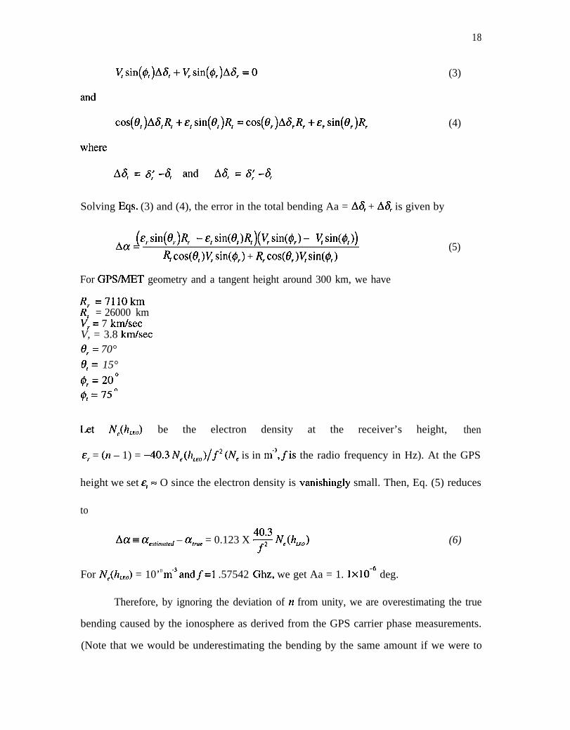
Solving Eqs. (3) and (4), the error in the total bending Aa = Ad + A6, is given by

Aa (~,sin(O,)R, -&,sin(Ot)~)(~sin(@,)- ~sin(@,))= (5)

~ COS(6,)~ sin(or) + R, COS(8,)~ sin(qj)

For GPSIMET geometry and a tangent height around 300 km, we have

R, =7110kmR, = 26000 kmV,= 7 kmfsecV, = 3.8 krn/sece,= 70°

q= 15°

(pr=200q,=75°

Let Zveo’zLEo) be the electron density at the receiver’s height, then

E, = (n – 1) = -40.3 ZVC(/Z~,,0)/~2 (N. is in m“3,~is the radio frequency in Hz). At the GPS

height we set e, = O since the electron density is vanishingly small. Then, Eq. (5) reduces

to

Aa = aev,i~,of,~ – (x,,U, = 0.123 X~ N~(hMO) (6)

For N,(h,KO) = 10’0 m-3 and~=l .57542 Ghz, we get Aa = 1. lxIO-G deg.

Therefore, by ignoring the deviation of n from unity, we are overestimating the true

bending caused by the ionosphere as derived from the GPS carrier phase measurements.

(Note that we would be underestimating the bending by the same amount if we were to

19

derive it from the GPS pseudorange measurements since 8, would have the opposite sign.)

Of importance is the bending error relative to the total bending. This fractional error can be

approximated by using the following simple model for the ionosphere. Let

( ‘-:”)N,(h) = Nnla exp – for h>h~,X and O otherwise,

where h~,u and Nn,~X correspond to the peak height and peak density respectively, H is the

free electron density scale height, Then, to a good approximation, the total bending for a

link with a tangent height h > hn,ax is given by (Melbourne et al., 1994, page 47)

rH’-FN-ex(-’-2)2zRa(h) =

where R~l~x = h~,dx + radius of earth. The fractional bending error is then given by

~(h)= 0“ 1 2 3

( )

h - h

r2nRnax

exp – ’60H

H

(7)

(6)

For hL.o = 740 km, Rn,ax = 6670 km, H = 70 km, we get

~(h) = 0.005expa (-hL’Hh)

Based on this exponential model and the GPWMET geometry, bending is overestimated by

less than 0.5% of the true one. In order to estimate the corresponding error in electron

density, we use the differential form of the Abel transform integral (Eq. (5a) of section 2)

which can be written as

An l“Aa cx da,J

—=——— (7)n n ~ a J=”

using Eq. (6) in (7) it is easy to establish that

(Nc)e~,inldt,d - (Ne),ru, < 0.123

r(Ne),rue - 2zRMAX = 0“ 005

H

(8)

This implies that the derived electron density is overestimated by no more than 0.5% of the

true density.

21

ACKNOWLEDGMENTS

We thank Mike Exner of UCAR for providing the GPS/MET flight data. We thank John

Foster for providing the Millstone Hill ISR data. Ionosonde data were provided by the

National Geophysical Data Center. This research was performed at the Jet Propulsion

Laboratory, California Institute of Technology, under the JPL Director’s Research

Discretionary Fund with partial funding from the National Science Foundation.

22

REFERENCES

Born M. and Wolf E., Principles of Optics, Sixth edition, Pergamon Press, 1980.

Daniell R. E., L, D. Brown, D. N. Anderson, M. W. Fox, P. H. Doherty, D. T. Decher,

J. J. Sojka, R. W. Schunk, “Parametrized Ionospheric Model-A global ionospheric

parametrization based on first principles models,” Radio Science, Vol. 30, No. 5, pp.

1499-1510, 1995.

Dekcer T. D., D. N. Anderson, R. M. Campbell, Simulations of GPS/MET Ionospheric

Observations, Amer. Geophy. Union fall meeting, Dec. 1996.

Fjeldbo G. F., V. R. Eshleman, A. J, Kliore, “The neutral atmosphere of Venus as studied

with the Mariner V radio occultation experiments;’ Astron. J. 76, pp. 123-140, 1971.

Gorbunov M. E., S. V. Sokolovsky, L, Bengtsson, Space Refractive Tomography of the

Atmosphere: Modeling of Direct and Inverse Problems, Max-Planck-Institut fur

Meteorologie, report No. 210, (ISSN 0937-1060), August, 1996.

Gurvich and Krasil’nikova, “Navigation Satellites for Radio Sensing of the Earth’s

Atmosphere”, Sov. J. of Remote Sensing, 7, pp. 1124-1131, 1990.—Russian Original

1987.

Hajj G. A., R. Ibanez-Meier, E. R. Kursinski and L. J. Remans, “Imaging the Ionosphere

with the Global Positioning System”, hzt. J. of Zmaging Sys. and Tech,, Vol. 5, 174-

184, 1994.

Hajj G. A., E. R. Kursinski, W. I. Bertiger, S. S. Leroy, and J. T. Schofield, “Sensing

the Atmosphere From a Low-Earth Orbiter Tracking GPS: Early Results and Lessons

From the GPS/MET Experiment,” Proc. of ION-GPS 95, The 8th International

Technical Meeting of The Satellite Division of The Institute of Navigation, pp 1167-

1174, 1995.

Hajj G. A., L, Remans, W. Bertiger, R. Kursinski and T. Mannucci, “Imaging the

ionosphere with GPS/MET”, proc. of the URSI GPSA14ET Workshop, Tucson,

Arizona, Feb. 21-24, 1996.

23

H@eg P., A. Hauchecorne, G. Kirchengast, S. Syndergaard, B. Belloul, R, Leitinger, W.

Rothleitner, Derivation of Atmospheric Properties Using . a Radio Occultation

Techniques, ESAZESTEC Contract Rep. 11024/94 flL/CN, DA41 Sci. Rep. 95-4,

edited by P. H@eg and S. Syndergaard, Danish Meteorol. Int,t., Copenhagen, 1995.

Kursinski E. R., G. A. Hajj, K. R, Hardy, L. J. Remans, and J. T. Schofield,

“Observing tropospheric water vapor by radio occultation using the global positioning

system,” Geophy. Res. Lett., Vol. 22, No. 17, pp. 2365-2368, 1995.

Kursinski E. R, G. A. Hajj, W. I. Bertiger, S. S. Leroy, T. K. Meehan, L. J. Remans, J.

T. Schofield, D. J. McCleese, W. G. Melbourne, C. L. Thornton, T. P. Yunck, J. R.

Eyre and R, N. Nagatani, “Initial Results of Radio Occultation Observations of Earth’s

Atmosphere Using the Global Positioning System,” Science, Vol. 271, pp. 1107-

1110, 1996.

Kursinski E. R., G. A. Hajj, K. R. Hardy, J. T. Schofield, and R. Linfield, “Observing

Earth’s Atmosphere with Radio Occultation Measurements using GPS,” J. Geophys.

Res., in press, 1997.

Leitinger R., H. P. Ladreiter and G. Kirchengast, “Ionosphere tomography with data from

satellite reception of global navigation satellites signals and ground reception of navy

navigation satellite system signals”, Radio Science, v32 (4), pp1657- 1669, 1997.

Leroy S., “The Measurement of Geopotential Heights by GPS Radio Occultation,”

submitted to J. Geophys. Res., Vol. 102, No. D6, pp. 6971-6986, 1997.

Mannucci A. J., B. D. Wilson, D. N. Yuan, C. M. Ho, U. J. Lindqwister, T. F. Runge,

“A Global Mapping Technique for GPS-Derived Ionospheric TEC Measurements:’

submitted to Radio Science, 1997.

Meehan T.K. et al., “The TurboRogue GPS Receiver”, 6th Int. Geodetic Symp. on

Satellite Positioning, Columbus Ohio, 1992.

Melbourne W. G., E. S. Davis, C. B. Duncan, G. A. Hajj, K. R. Hardy, E. R.

Kursinski, T. K, Meehan, L. E. Young, T. P. Yunck, The Application of Spaceborne

24

GPS to Atmospheric Limb Sounding and Global Change Monitoring, Jet Propulsion

Laboratory publication 94-18, April 1994.

Tricomi F. G., Integral Equations, Dover Publications, Inc., New York, 1985.

Tyler G. L., “Radio propagation experiments in the outer solar system with Voyager,”

Proc. ZEEE, 75:1404-1431, 1987.

Ware R., M. Exner, D. Feng, M. Gorbunov, K. Hardy, B. Herman, Y. Kuo, T. Meehan,

W. Melbourne, C. Rocken, W. Schreiner, S. $okolovskiy, F. Solheim, X. Zou, R.

Anthes, S. Businger, and K. Trenberth. “GPS sounding of the atmosphere from low

earth orbit: preliminary results,” Bulletin of the American Meteorological Society, Vol.

77, No. 1, pp. 19-40, 1996.

Yunck T. P., G. F. Lindal and C, H, Liu, “The Role of GPS in precise earth observation~’

in Proceedings of the IEEE Position, Location and Navigation Symposium, Orlando,

Florida, 1988.

25

FIGURE CAPTIONS

Figure 1: Occultation geometry defining a, r, sand the tangent point and showing the

separation of the L 1 and L2 signals due to the dispersive ionosphere.

Figure 2: Bending induced by the ionosphere and neutral atmosphere on the L1 signal for

61 globally distributed occultations on May 4, 1995. Negative bending is defined to be

toward the Earth’s center.

Figure 3: Electron density retrieved from occultation and the corresponding amount of L1

and L2 signal vertical separation at the tangent point.

Figure 4: Instrumental signal-to-noise ratio as a function of time for L1 and L2 signals for

four different occultations.

Figure 5: GPWMET profiles of electron density corresponding to the occultations of Fig. 4

and indicating the ability of GPS occultations to resolve sharp layers in the ionosphere.

Figure 6. (a) GPWMET coverage in geographic coordinates for 20 days (April 24 and 25,

May 3 and 4, June 21-24 and 27-30, July 1-7 of 1995). Each dot indicates the location of

the tangent point of the occultation when it is at -100 km altitude. The triangles indicate

locations of ionosonde stations used in order to compare to N~Fz derived from GPWMET.

(b) GPSM4ET coverage in sun-fixed coordinates in 24 hours, May 4, 1995. Each

connected line corresponds to the ground projection of an occultation link when the tangent

point (middle of the line) is at 100 km altitude. The ends of the line correspond to points

on that same link at 400 km altitudes. At low latitude, the occultations sample roughly the

same local time and same latitude every orbital revolution. The circle indicates four

26

occultations corresponding to four consecutive orbital revolutions (-100 minutes apart); the

corresponding profiles are shown in Fig. 7a.

Figure 7: Examples of electron density profiles (e/ms) obtained from GPWMET and PIM

for May 4, 1995. (a): low latitudes profiles (b): high latitudes profiles. Indicated on the

top of each profile are universal time, local time, latitude and longitude of each occultation.

Figure 8: Comparisons of an electron density profile obtained from GPWMET on May 5,

1995,0320 UT, with nearby measurements from Millstone Hill ISR. (a): GPSIMET vs.

two ISR measurements with 640 ps pulse mode at 0321 UT and 0340 UT. (b) GPWMET

vs. ISR measurements with 320 ps pulse mode at 0341 UT. The occultation tangent point

is about 6° west and 1° south of Millstone Hill.

Figure 9a: A scatter plot of N~Fz derived from ionosonde measurements of FOFZ, and

GPMMET electron density profiles, showing the degree of correlation between the two.

The middle line corresponds to perfect correlation; the upper and lower lines bound of the

region of 20% deviation in the two measurements.

Figure 9.b: The fractional difference between N~F2 derived from GPS/MET and the

ionosonde (defined in Eq. (7)) as a function of the distance between the station and the

tangent point of the occultation. Differences that are larger than -0.5 can be attributed to

the large distance between the station and the occultation.

Figure 10: Histogram of the fractional difference between N~Fz derived from GPWMET

and the ionosonde for measurements within 1 hour and 600 km from each other. Average

and standard deviation are 0.01 and 0.20 respectively. Based on this histogram, the two

2-I

independent measurements of N~Fz agree to within 209To (1-sigma) and are essential

unbiased.

Figure A: Geometry showing the direct line-of-sight

the asymptotes of transmitted and received signals.

between transmitter and receiver and

L2 Signal

GPS

LEO

29

Ex

700

600

500

400

300

200

100

0

1 I I I I 6

I

LI i 1 1 1 * I n ,

-0.03 -0.02 -0.01 0 0.01 0.02 0.03

Bending, deg

Figure 2

30

Tangent Point Difference, L1 -L2, meters

-400 -300 -200 -100 0 100 200 300600

Tangent Point Diff{ went

500

400

Electron Density

300

200

100

00 0.1 0.2 0.3 0.4 0.5 0.6 0.7

\

Free Electron Density, e/m3xlO’2

Figure 3

31

L1 Signal

600 ~. . ~~ L2 Signal

1 I I I I500 Date: 1995-05-04

UT: 0929400 LT: 0116m

5Lat -34N, Lon 236E

200

0

500400

% 300Co

200100

0

500400

az 300u)200100

0

500400

1000 0 10 20 30 40 50 60

Time, Sec.

Figure 4

32

600 1=-.=. 1. -

500 - Lat -34N, Lon 236E;

400 -Exz- 300 -@+!

200 -

100 -

o~lollo

600

500

400

300

200

100

—l . . . ..~ . . . . . . . . . . .

Date 1995-05-04UT: 1928

Lat -36N, Lon 88E I

-1

Electron density, m-3 Electron density, m-3

600Date 1995-05-04UT: 1125

500 - Lat -55N, Lon 296E~

400 -

E : 5

Q - E. ,Q$ . 2

200 -

100 “

r co~

o 110” 1.510’

Electron density, m-3

500 -

400 -

300 -

200 -

100 -

, o~o 2 1 0 ” 4 1 0 ” 6 1 0 ”

Electron density, m-3

Figure 5

I ,1 I 1 1 1 1

90

60

30

0

-30

-60

-180 -120 -60 0 60 120 180

Geographic Longitude

(a)

-90-1 Ilo -lho -do 6 6’0 140 140

Sun-Fixed Longitude, deg

(b)

Figure 6

34ELECTRON DENSITY PROFILES FROM GPS/MET AND THE

PARAMETRIZED IONOSPHERIC MODELOBTAINED FOR MAY 4, 1995 AT ABOUT THE SAME LATITUDE AND LOCAL TIME

600

500

~ 400xx$ 300I

200

100

— G P S / M E T-----PIM

18:27 UT 20:04 UT11:43 LT 11:12LT

259.1 E,3.5N 227 E, -3.3 N

OLJ—MLuA10’ 0 lo” 10’

10:34 UT 18:53 UT18:34 LT 18:53 LT

0E,67N

xz~ 3oo-

2 2oo- ,/’,.’---------

()~1 09 1 0 ’0 l o ” 109 10’0 1 0 ”

! I UilL

2 10’ 0 10” 10’2

21:46 UT 23:24 UT11:29 LT 11:12LT

208.3 E, 2.8 N 177 E, -1.1 N

2,’

4

1’

10’ 0 10” 1(

Electrot_(~ensity, e/mA3

—-----

13:54 UT19:06 LT

78 E, 68 N

J

‘!‘,

‘,‘!:

..’. .-..

:;:;: ::

319 E,68N

D

‘1;\\‘1

‘1‘1

,’,’.*. . . .

17:16 UT21:06 LT

58 E, 69 N

D

:‘1‘,

‘1

#,’

,’.’. ...---”’

LJAJwLA~1(Y 1010 1011 ld 1010 1011 109 1010 1011

l!.l,l t I2 10’ 0 10” 10’2

07:18 UT ());; :;21:48 LT :

218 E, 70N 263 E, 61 N

\

,

:.

, d d —~ 10’0 l o ” 1(Y 10’0 1 0 ”

(b)

Figure 7

600

500

400

300

200

100

00

600 <

500

400

300[L

200

100

510’0 1 lo” 1.510” 2 1 0 ”

Electron Density (m”3)

(a)

oh 1 , , 1

0 5 1 0 ’0 1 10” 1.510” 210’

Electron Density (m-3)

(b)

Figure 8

36

1.410’2

1.210’2

1 10’2

8 1 0 ”

6 1 0 ”

4 1 0 ”

2 1 0 ”

0o 21011 41011 610fi 81011 1 1012 1.2101 z1.4101z

N~F2 (Ionosonde), e/m3

Fig. 9.a

1.5

1

0.5

0

-0.5

-1

. . . . . . . . . . . . . . . . . . . . .

. . . . . . . . . . . . . . . . . . . . .

●

✎ ✎ ✎ ✎ ✎ ✎ ✎ ✎ ✎ ✎ ✎ ✎ ✎ ✎ ✎ ✎ ✎ ✎ ✎ ✎ ✎

●

✎ ✎ ✎ ✎ ✎ ✎ ✎ ✎ ✎ ✎ ✎ ✎ ✎ ✎ ✎ ✎ ✎ ✎ ✎ ✎ ✎

o 2

:0● ● {*

? r. . . . . . . . . ...+. . . . . . . . . . . . . . . . . . . . . . . . . .@ q● * # ,,

●.;●

● ●

:0

}●

. . . . . . . . . . . . . . . . . . . . . . . . . . . . . . . . . . . . . . . . . . . . . . .

;0●

~

<. . . . . . . . . . . . . . . . . . . . . . . . . . . . . . . . . . . . . . . . . . . . ...!

● i

●

•~.

●

● *!. . ..~ . . . . . . . . . . . . . .. f................... ”....

● :‘ e .* 8

● ● ; :8 ‘● ; ●

● *. ● *% : .

~:”

●

~D 400 600 800 1000 1:

---L---

●

✎ ✎ ✎ ✎ ✎ ✎ ✎ ✎ ✎ ✎ ✎ ✎ ✎ ✎ ✎ ✎ ✎ ✎ ✎ ✎ ✎

✎ ✎ ✎ ✎ ✎ ✎ ✎ ✎ ✎ ✎ ✎ ✎ ✎ ✎ ✎ ✎ ✎ ✎ ✎ ✎ ✎

●

●

✎ ✎ ✎ ✎ ✎ ✎ ✎ ✎ ✎ ✎ ✎ ✎ ✎ ✎ ✎ ✎ ✎ ✎ ✎ ✎ ✎

Bs

●

●

. . . . . . . . . . . . . . . . . . . . .

Separation distance between occultation and ionosonde, km

Fig. 9.b

38

12

10

8

6

4

2

0-0.6 -0.4 -0.2 0 0.2 0.4 0.6

( NmF2(abel) - NmF2(ionosonde) )/NmFp(ionosonde)

Fig. 10

39

AVt @k

@r

Rt

Fig. A