Embed Size (px)
Citation preview
ISTANBUL TECHNICAL UNIVERSITY EARTHQUAKE ENGINEERING AND DISASTER
MANAGEMENT INSTITUTE
M.Sc. THESIS
MAY 2017
ANALYSIS OF DYNAMIC RESPONSE AND INSTABILITY OF A CAISSON
TYPE GRAVITY QUAY WALL – SEABED SYSTEM UNDER WAVES
Thesis Advisor: Assoc. Prof. Dr. Mehmet BarıĢ Can ÜLKER
Hasan Giray BAKSI
Earthquake Engineering and Disaster Management Institute
Earthquake Engineering Program

Earthquake Engineering and Disaster Management Institute
Earthquake Engineering Program
MAY 2017
ISTANBUL TECHNICAL UNIVERSITY EARTHQUAKE ENGINEERING AND DISASTER
MANAGEMENT INSTITUTE
ANALYSIS OF DYNAMIC RESPONSE AND INSTABILITY OF A CAISSON
TYPE GRAVITY QUAY WALL – SEABED SYSTEM UNDER WAVES
M.Sc. THESIS
Hasan Giray BAKSI
(802121017)
Thesis Advisor: Assoc. Prof. Dr. Mehmet BarıĢ Can ÜLKER


Deprem Mühendisliği Anabilim Dalı
Deprem Mühendisliği Programı
MAYIS 2017
ĠSTANBUL TEKNĠK ÜNĠVERSĠTESĠ DEPREM MÜHENDĠSLĠĞĠ VE AFET
YÖNETĠMĠ ENSTĠTÜSÜ
KESON TĠPĠ RIHTIM DUVARI – DENĠZ TABANI SĠSTEMĠNĠN
DALGA ETKĠLERĠ ALTINDAKĠ DĠNAMĠK TEPKĠSĠ VE DURAYSIZLIĞININ
ĠNCELENMESĠ
YÜKSEK LĠSANS TEZĠ
Hasan Giray BAKSI
(802121017)
Tez DanıĢmanı: Doç. Dr. Mehmet BarıĢ Can ÜLKER

v
Thesis Advisor : Assoc. Prof. Dr. Mehmet BarıĢ Can ÜLKER ...................
Istanbul Technical University
Co-advisor : Doç.Dr. Veysel ġadan Özgür KIRCA ..............................
(If exists) ISTANBUL Technical University
Jury Members : Assoc. Prof. Dr. Mehmet BarıĢ Can ÜLKER ...................
Istanbul Technical University
Assoc. Prof. Dr. Veysel ġadan Özgür KIRCA ...................
Istanbul Technical University
Asst. Prof. Dr. Gökçe TÖNÜK ..............................
MEF University
(If exists) Prof. Dr. Name SURNAME ..............................
Hospital
(If exists) Prof. Dr. Name SURNAME ..............................
University
Hasan Giray BAKSI, a M.Sc. student of ITU Earthquake Engineering and Disaster
Management Institute student ID 802121017, successfully defended the thesis
entitled “ANALYSIS OF DYNAMIC RESPONSE AND INSTABILITY OF A
CAISSON TYPE GRAVITY QUAY WALL – SEABED SOIL SYSTEM UNDER
WAVES”, which he prepared after fulfilling the requirements specified in the
associated legislations, before the jury whose signatures are below.
Date of Submission : 04 May 2017
Date of Defense : 17 May 2017

vi

vii
To my family,

viii
ix
FOREWORD
First of all, I would like to express my deep gratitude to Dr. Ulker, my research
advisor, for his patience, guidance and useful critiques during this research work. His
labor was not less than mine to make a high-quality thesis, certainly. I would also
like to thank Dr. Kirca for their critical recommendation and support that made this
research possible.
Especially to Belgin, my wife, thanks for giving me your patience, encouragement
and love even in hard times during this period.
May 2017
Hasan Giray BAKSI
(Civil Engineer)

x
xi
TABLE OF CONTENTS
Page
FOREWORD ............................................................................................................. ix TABLE OF CONTENTS .......................................................................................... xi
ABBREVIATIONS ................................................................................................. xiii SYMBOL LIST ........................................................................................................ xv LIST OF TABLES .................................................................................................. xix
LIST OF FIGURES ................................................................................................ xxi SUMMARY ............................................................................................................ xxv ÖZET ............................................................................................................ xxvii 1. INTRODUCTION .................................................................................................. 1
2. LITERATURE REVIEW ..................................................................................... 5 2.1 Quay Walls as Marine Structures ....................................................................... 5 2.2 Poroelasticity in the Analysis of Coastal and Marine Structures ....................... 5
2.3 Liquefaction Studies. .......................................................................................... 7
3. MATHEMATICAL FORMULATION OF POROELASTICITY:
DYNAMICS OF SATURATED POROUS SEABED ......................... 9 3.1 Governing Equations ........................................................................................ 10
3.2 Simplified Forms .............................................................................................. 12
4. NUMERICAL FORMULATION ....................................................................... 15 4.1 Finite Element Formulations ............................................................................ 15
5. FINITE ELEMENT ANALYSES: DETAILS ................................................... 17 5.1 Spatial Integration ............................................................................................ 17
5.1.1 Gauss quadrature ....................................................................................... 17 5.1.2 Shape functions ......................................................................................... 18
5.2 Temporal Integration ........................................................................................ 21 5.2.1 Implicit Newmark - β Method .................................................................. 21
6. VERIFICATION ANALYSES ........................................................................... 23 6.1 Problem 1: One-Dimensional Soil Column Response under Cyclic Wave ..... 23
6.1.1 Problem definition ..................................................................................... 23 6.1.2 Boundary conditions ................................................................................. 25 6.1.3 Results on the analyses for 1-D soil column ............................................. 25
6.2 Problem 2: Two-Dimensional Seabed Layer Response under Progressive Wave
Loading ................................................................................................................... 27 6.2.1 Problem definition ..................................................................................... 27 6.2.2 Stress calculation ....................................................................................... 27 6.2.3 Boundary conditions ................................................................................. 28
6.2.4 Finite element model ................................................................................. 30
7. DYNAMIC RESPONSE ANALYSIS OF CAISSON TYPE QUAY WALL
(CTQ) - SEABED SYSTEM UNDER STANDING WAVES ........... 35 7.1 Introduction ...................................................................................................... 35 7.2 Finite Element Analyses ................................................................................... 35
xii
7.3 Results of Analyses .......................................................................................... 39 7.3.1 Effect of seabed permeability .................................................................... 39 7.3.2 Effect of seabed soil type .......................................................................... 51 7.3.3 Effect of standing wave period .................................................................. 63
8. INSTABILITY OF CTQ - SEABED SYSTEM UNDER STANDING WAVES
................................................................................................................ 75 8.1 Instantaneous Liquefaction ............................................................................... 76 8.2 Numerical Analysis of Liquefaction ................................................................ 78 8.3 Parametric Study Results .................................................................................. 80
8.3.1 Effect of seabed permeability .................................................................... 81 8.3.2 Effect of seabed soil type .......................................................................... 81 8.3.3 Effect of standing wave period .................................................................. 82
8.4 Shear Stress Variations ..................................................................................... 82 8.4.1 Effect of seabed permeability .................................................................... 82 8.4.2 Effect of seabed soil type .......................................................................... 83 8.4.3 Effect of standing wave period .................................................................. 84
8. CONCLUSIONS................................................................................................... 99 9. FUTURE WORKS ............................................................................................. 101 REFERENCES ....................................................................................................... 103
APPENDICES ........................................................................................................ 109 APPENDIX A The liquefaction hazards at Kobe Port. ........................................ 109 APPENDIX B Views and maps. .......................................................................... 113
CURRICULUM VITAE ........................................................................................ 117

xiii
ABBREVIATIONS
ASTM : American Society for Testing and Materials International
CTQ : Caisson Type Quay Wall
DOF : Degree of Freedom
FD : Fully Dynamic
FE : Finite Elements
FEM : Finite Element Method
GM : Silty Gravel
GW : Well Graded Gravel
MPC : Multi Point Constraint
SP : Poorly Graded Sand
PD : Partly Dynamic
QS : Quasi Static
Q4 : Quadrilateral 4-noded
Q8 : Quadrilateral 8-noded
USCS : Unified Soil Classification System
1-D : One Dimensional
2-D : Two Dimensional
3-D : Three Dimensional

xiv
xv
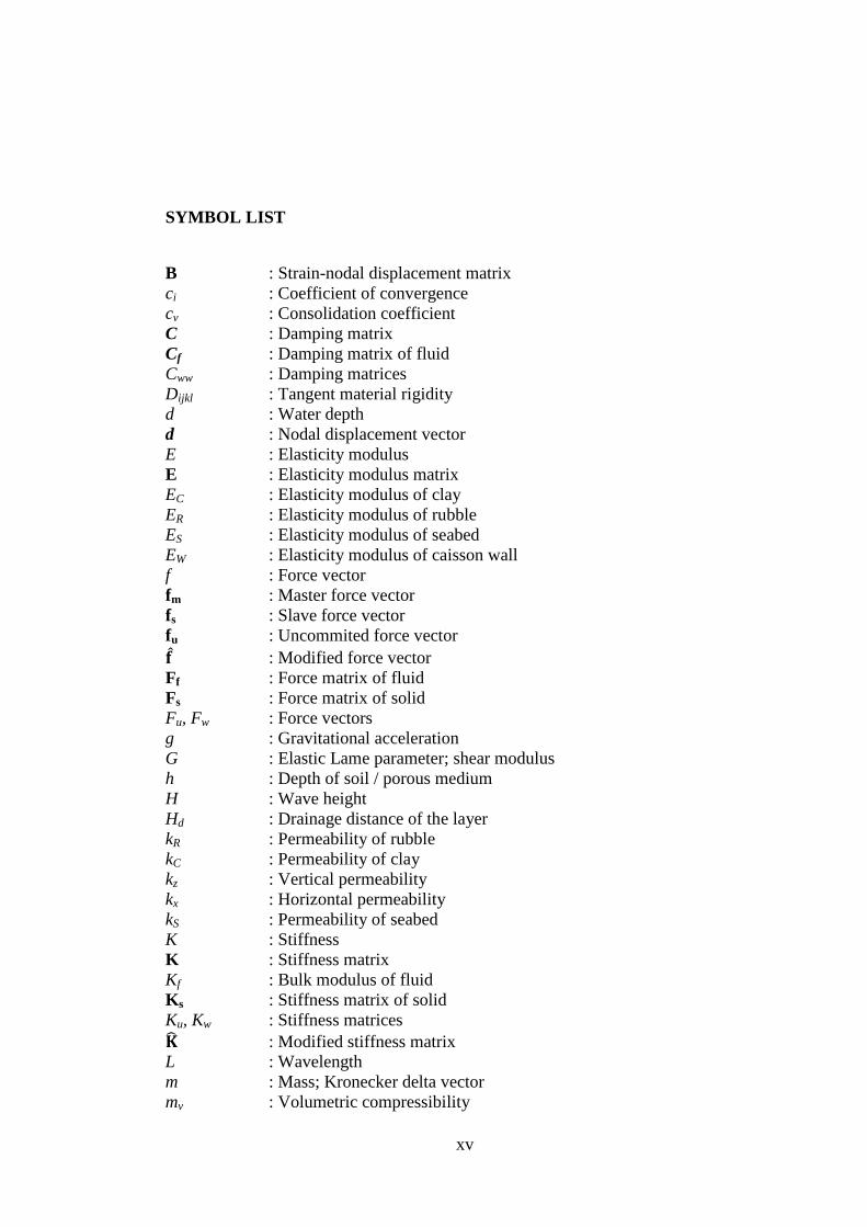
SYMBOL LIST
B : Strain-nodal displacement matrix
ci : Coefficient of convergence
cv : Consolidation coefficient
C : Damping matrix
Cf : Damping matrix of fluid
Cww : Damping matrices
Dijkl : Tangent material rigidity
d : Water depth
d : Nodal displacement vector
E : Elasticity modulus
E : Elasticity modulus matrix
EC : Elasticity modulus of clay
ER : Elasticity modulus of rubble
ES : Elasticity modulus of seabed
EW : Elasticity modulus of caisson wall
f : Force vector
fm : Master force vector
fs : Slave force vector
fu : Uncommited force vector
: Modified force vector
Ff : Force matrix of fluid
Fs : Force matrix of solid
Fu, Fw : Force vectors
g : Gravitational acceleration
G : Elastic Lame parameter; shear modulus
h : Depth of soil / porous medium
H : Wave height
Hd : Drainage distance of the layer
kR : Permeability of rubble
kC : Permeability of clay
kz : Vertical permeability
kx : Horizontal permeability
kS : Permeability of seabed
K : Stiffness
K : Stiffness matrix
Kf : Bulk modulus of fluid
Ks : Stiffness matrix of solid
Ku, Kw : Stiffness matrices
: Modified stiffness matrix
L : Wavelength
m : Mass; Kronecker delta vector
mv : Volumetric compressibility
xvi
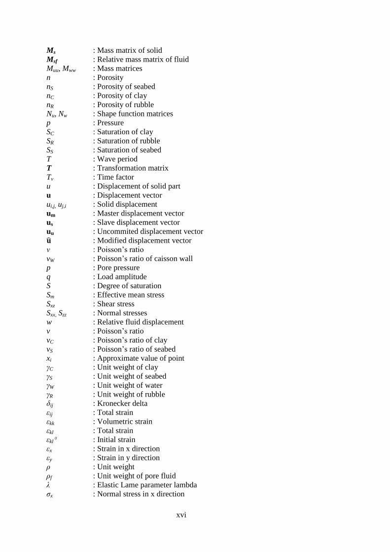
Ms : Mass matrix of solid
Msf : Relative mass matrix of fluid
Muu, Mww : Mass matrices
n : Porosity
nS : Porosity of seabed
nC : Porosity of clay
nR : Porosity of rubble
Nu, Nw : Shape function matrices
p : Pressure
SC : Saturation of clay
SR : Saturation of rubble
SS : Saturation of seabed
T : Wave period
T : Transformation matrix
Tv : Time factor
u : Displacement of solid part
u : Displacement vector
ui,j, uj,i : Solid displacement
um : Master displacement vector
us : Slave displacement vector
uu : Uncommited displacement vector
: Modified displacement vector
ν : Poisson‟s ratio
vW : Poisson‟s ratio of caisson wall
p : Pore pressure
q : Load amplitude
S : Degree of saturation
Sm : Effective mean stress
Sxz : Shear stress
Sxx, Szz : Normal stresses
w : Relative fluid displacement
v : Poisson‟s ratio
vC : Poisson‟s ratio of clay
vS : Poisson‟s ratio of seabed
xi : Approximate value of point
γC : Unit weight of clay
γS : Unit weight of seabed
γW : Unit weight of water
γR : Unit weight of rubble
δij : Kronecker delta
εij : Total strain
εkk : Volumetric strain
εkl : Total strain
εkl 0 : Initial strain
εx : Strain in x direction
εy : Strain in y direction
ρ : Unit weight
ρf : Unit weight of pore fluid
λ : Elastic Lame parameter lambda
ζx : Normal stress in x direction
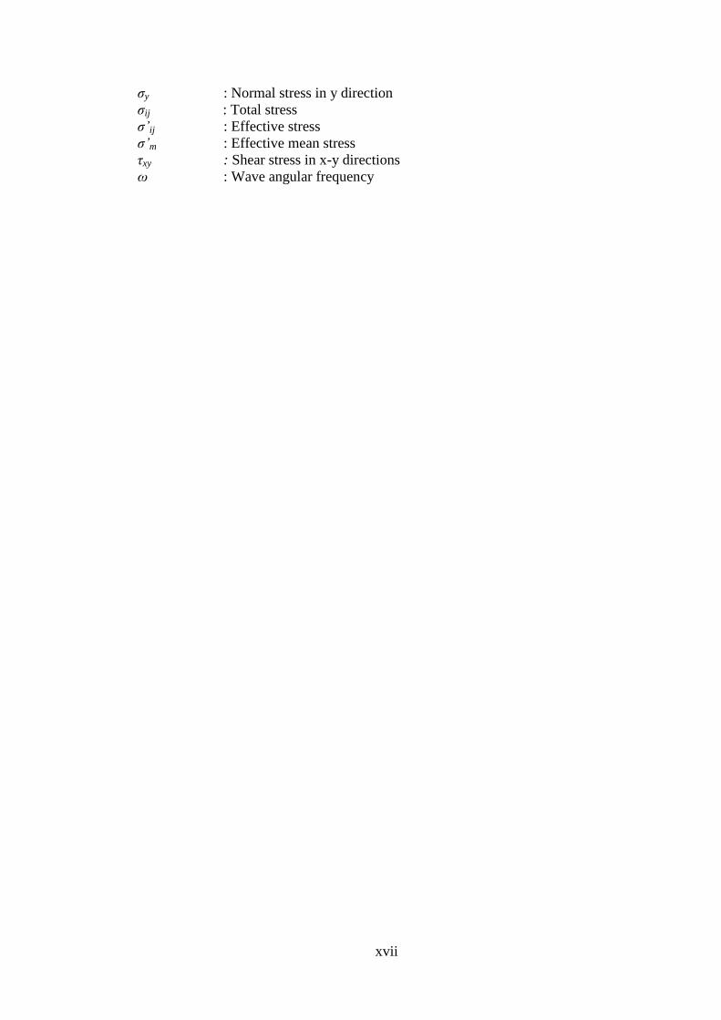
xvii
ζy : Normal stress in y direction
ζij : Total stress
ζ’ij : Effective stress
ζ’m : Effective mean stress
ηxy : Shear stress in x-y directions
ω : Wave angular frequency

xviii
xix
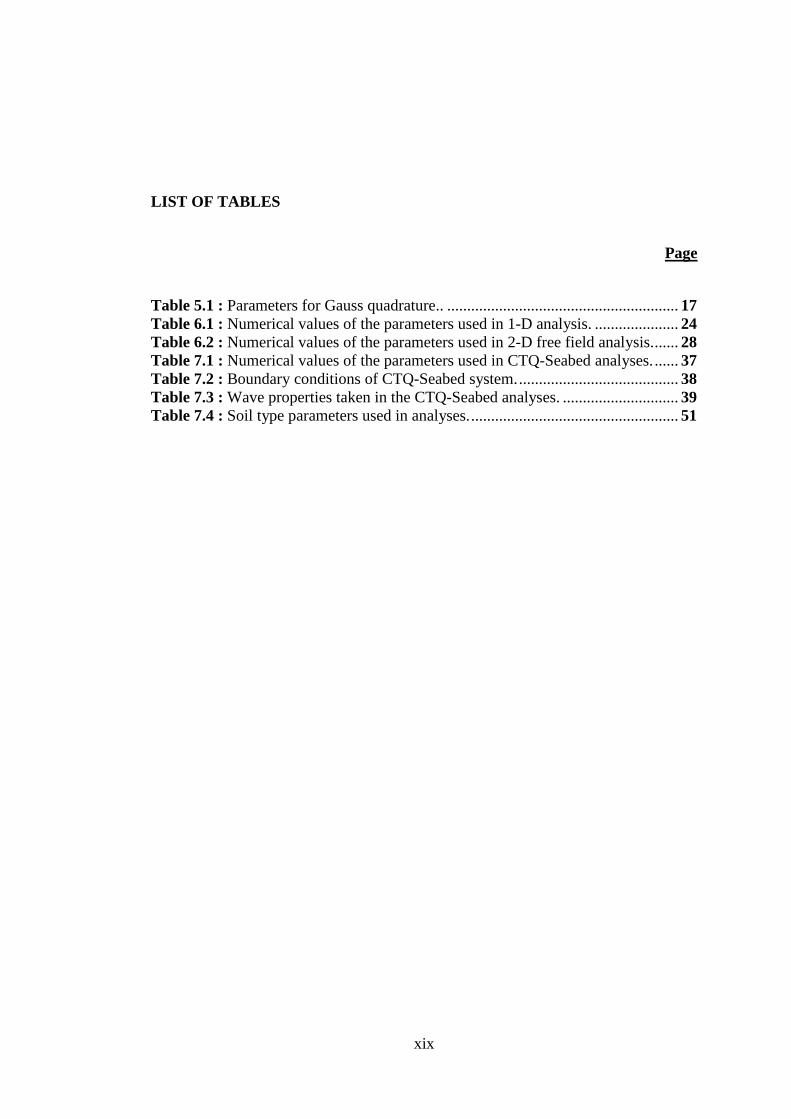
LIST OF TABLES
Page
Table 5.1 : Parameters for Gauss quadrature.. .......................................................... 17
Table 6.1 : Numerical values of the parameters used in 1-D analysis. ..................... 24
Table 6.2 : Numerical values of the parameters used in 2-D free field analysis. ...... 28
Table 7.1 : Numerical values of the parameters used in CTQ-Seabed analyses. ...... 37 Table 7.2 : Boundary conditions of CTQ-Seabed system. ........................................ 38 Table 7.3 : Wave properties taken in the CTQ-Seabed analyses. ............................. 39
Table 7.4 : Soil type parameters used in analyses. .................................................... 51

xx
xxi
LIST OF FIGURES
Page
Figure 5.1 : Quadrilateral 8-noded (Q8) ................................................................... 18
Figure 5.2 : Quadrilateral 4-noded (Q4) ................................................................... 19
Figure 5.3 : Basic FEM features used in analyses .................................................... 20
Figure 6.1 : Reaching steady state for any point on soil column .............................. 24
Figure 6.2 : Boundary conditions for 1-D soil column ............................................. 25
Figure 6.3 : Vertical displacements by elevation for 1-D soil column ..................... 26
Figure 6.4 : Pore pressure by elevation for 1-D soil column .................................... 26 Figure 6.5 : A layer of saturated porous seabed under progressive wave loading .... 27
Figure 6.6 : Progressive wave seabed system with boundary conditions ................. 29
Figure 6.7 : FE mesh ................................................................................................. 31
Figure 6.8 : Convergence check by pore pressure variations in depth ..................... 31
Figure 6.9 : Vertical displacement variation by depth in PD solution. ..................... 32
Figure 6.10 : Pore pressure variation by depth in PD solution. ................................ 32
Figure 6.11 : Effective vertical stress by depth in PD solution................................. 33
Figure 7.1 : Physical model of CTQ at the Kobe Port and relevant sections............ 38 Figure 7.2 : CTQ – Kobe Port FE mesh and material zones ..................................... 38 Figure 7.3 : Effect of permeability on horizontal displacement in section 1-1 ......... 40
Figure 7.4 : Effect of permeability on vertical displacement in section 1-1 ............. 41 Figure 7.5 : Effect of permeability on pore pressure in section 1-1.......................... 41
Figure 7.6 : Effect of permeability on vertical displacement in section 2-2 ............. 42
Figure 7.7 : Effect of permeability on pore pressure in section 2-2.......................... 43
Figure 7.8 : Effect of permeability on horizontal displacement in section 3-3 ......... 45 Figure 7.9 : Effect of permeability on vertical displacement in section 3-3 ............. 45
Figure 7.10 : Effect of permeability on pore pressue in section 3-3 ......................... 46 Figure 7.11 : Effect of permeability on normal stress in x direction in section 1-1 . 46
Figure 7.12 : Effect of permeability on normal stress in z direction in section 1-1 .. 47
Figure 7.13 : Effect of permeability on shear stress in section 1-1 ........................... 47
Figure 7.14 : Effect of permeability on normal stress in x direction in section 2-2 . 48 Figure 7.15 : Effect of permeability on normal stress in z direction in section 2-2 .. 48 Figure 7.16 : Effect of permeability on shear stress in section 2-2 ........................... 49
Figure 7.17 : Effect of permeability on normal stress in x direction in section 3-3 . 49 Figure 7.18 : Effect of permeability on normal stress in z direction in section 3-3 .. 50 Figure 7.19 : Effect of permeability on shear stress in section 3-3 ........................... 50
Figure 7.20 : Effect of soil type on horizontal displacement in section 1-1 ............. 53 Figure 7.21 : Effect of soil type on vertical displacement in section 1-1 ................. 53
Figure 7.22 : Effect of soil type on pore pressure in section 1-1 .............................. 54 Figure 7.23 : Effect of soil type on vertical displacement in section 2-2 ................. 55
Figure 7.24 : Effect of soil type on pore pressure in section 2-2 .............................. 56 Figure 7.25 : Effect of soil type on horizontal displacement in section 3-3 ............. 56 Figure 7.26 : Effect of soil type on vertical displacement in section 3-3 ................. 58
xxii
Figure 7.27 : Effect of soil type on pore pressue in section 3-3 ................................ 58 Figure 7.28 : Effect of soil type on normal stress in x direction in section 1-1 ........ 59 Figure 7.29 : Effect of soil type on normal stress in z direction in section 1-1 ........ 59 Figure 7.30 : Effect of soil type on shear stress in section 1-1 ................................. 60
Figure 7.31 : Effect of soil type on normal stress in x direction in section 2-2 ........ 60 Figure 7.32 : Effect of soil type on normal stress in z direction in section 2-2 ........ 61 Figure 7.33 : Effect of soil type on shear stress in section 2-2 ................................. 61 Figure 7.34 : Effect of soil type on normal stress in x direction in section 3-3 ........ 62 Figure 7.35 : Effect of soil type on normal stress in z direction in section 3-3 ........ 62
Figure 7.36 : Effect of soil type on shear stress in section 3-3 ................................. 63 Figure 7.37 : Effect of wave period on horizontal displacement in section 1-1 ....... 64 Figure 7.38 : Effect of wave period on vertical displacement in section 1-1 ............ 64
Figure 7.39 : Effect of wave period on pore pressure in section 1-1 ........................ 65 Figure 7.40 : Effect of wave period on vertical displacement in section 2-2 ............ 66 Figure 7.41 : Effect of wave period on pore pressure in section 2-2 ........................ 67 Figure 7.42 : Effect of wave period on horizontal displacement in section 3-3 ....... 68
Figure 7.43 : Effect of wave period on vertical displacement in section 3-3 ............ 69 Figure 7.44 : Effect of wave period on pore pressue in section 3-3 .......................... 70 Figure 7.45 : Effect of wave period on normal stress in x direction in section 1-1 .. 70 Figure 7.46 : Effect of wave period on normal stress in z direction in section 1-1 .. 71
Figure 7.47 : Effect of wave period on shear stress in section 1-1 ........................... 71 Figure 7.48 : Effect of wave period on normal stress in x direction in section 2-2 .. 72
Figure 7.49 : Effect of wave period on normal stress in z direction in section 2-2 .. 72 Figure 7.50 : Effect of wave period on shear stress in section 2-2 ........................... 73
Figure 7.51 : Effect of wave period on normal stress in x direction in section 3-3 .. 73 Figure 7.52 : Effect of wave period on normal stress in z direction in section 3-3 .. 74
Figure 7.53 : Effect of wave period on shear stress in section 3-3 ........................... 74 Figure 8.1 : Pore pressure builds up and accumulation ............................................ 76 Figure 8.2 : Instantaneous liquefaction caused by waves (De Groot et al., 2006) .... 78
Figure 8.3 : Time history for loads in wave induced response; hydrostatic load
followed by standing wave applied on seaward boundary ..................... 79
Figure 8.4 : Sm, σ‟m contours for SP, T=5 s, ks=10E-6 m/s, a)QS b)PD ................. 85
Figure 8.5 : Sm, σ‟m contours for SP, T=10 s, ks=10E-2 m/s, a)QS b)PD ............... 86 Figure 8.6 : Sm, σ‟m contours for SP, T=10 s, ks=10E-4 m/s, a)QS b)PD ............... 87
Figure 8.7 : Sm, σ‟m contours for GM, T=10 s, ks=10E-6 m/s, a)QS b)PD ............. 88 Figure 8.8 : Sm, σ‟m contours for SP, T=10 s, ks=10E-6 m/s, a)QS b)PD ............... 89
Figure 8.9 : Sm, σ‟m contours for GW, T=10 s, ks=10E-6 m/s, a)QS b)PD ............. 90 Figure 8.10 : Sm, σ‟m contours for SP, T=15 s, ks=10E-6 m/s, a)QS b)PD ............. 91 Figure 8.11 : σxz contours for SP, T=5 s, ks=10E-6 m/s, a)QS b)PD ........................ 92 Figure 8.12 : σxz contours for SP, T=10 s, ks=10E-2 m/s, a)QS b)PD ...................... 93 Figure 8.13 : σxz contours for SP, T=10 s, ks=10E-4 m/s, a)QS b)PD ...................... 94
Figure 8.14 : σxz contours for GM, T=10 s, ks=10E-6 m/s, a)QS b)PD .................... 95 Figure 8.15 : σxz contours for SP, T=10 s, ks=10E-6 m/s, a)QS b)PD ...................... 96 Figure 8.16 : σxz contours for GW, T=10 s, ks=10E-6 m/s, a)QS b)PD .................... 97 Figure 8.17 : σxz contours for SP, T=15 s, ks=10E-6 m/s, a)QS b)PD ...................... 98 Figure A.1 : Aerial photograph of collapsed crene. ................................................ 109
Figure A.2 : Aerial photograph of Port Island in Kobe ........................................... 109
Figure A.3 : Ferry ramp collapse. ........................................................................... 110 Figure A.4 : Graben behind quay wall. ................................................................... 110 Figure A.5 : Quay wall along channel .................................................................... 111

xxiii
Figure A.6 : Submerged pier. .................................................................................. 112 Figure B.1 : Satellite view of Port Island, Kobe Port.. ........................................... 113 Figure B.2 : Map of Port Island, Kobe Port.. .......................................................... 114 Figure B.3 : Aerial view of Ambarli Port, Istanbul. ............................................... 115

xxiv
xxv
ANALYSIS OF DYNAMIC RESPONSE AND INSTABILITY OF A CAISSON
TYPE GRAVITY QUAY WALL – SEABED SYSTEM UNDER WAVES
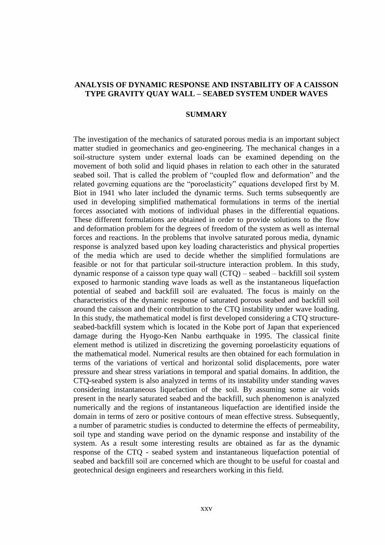
SUMMARY
The investigation of the mechanics of saturated porous media is an important subject
matter studied in geomechanics and geo-engineering. The mechanical changes in a
soil-structure system under external loads can be examined depending on the
movement of both solid and liquid phases in relation to each other in the saturated
seabed soil. That is called the problem of “coupled flow and deformation” and the
related governing equations are the “poroelasticity” equations developed first by M.
Biot in 1941 who later included the dynamic terms. Such terms subsequently are
used in developing simplified mathematical formulations in terms of the inertial
forces associated with motions of individual phases in the differential equations.
These different formulations are obtained in order to provide solutions to the flow
and deformation problem for the degrees of freedom of the system as well as internal
forces and reactions. In the problems that involve saturated porous media, dynamic
response is analyzed based upon key loading characteristics and physical properties
of the media which are used to decide whether the simplified formulations are
feasible or not for that particular soil-structure interaction problem. In this study,
dynamic response of a caisson type quay wall (CTQ) – seabed – backfill soil system
exposed to harmonic standing wave loads as well as the instantaneous liquefaction
potential of seabed and backfill soil are evaluated. The focus is mainly on the
characteristics of the dynamic response of saturated porous seabed and backfill soil
around the caisson and their contribution to the CTQ instability under wave loading.
In this study, the mathematical model is first developed considering a CTQ structure-
seabed-backfill system which is located in the Kobe port of Japan that experienced
damage during the Hyogo-Ken Nanbu earthquake in 1995. The classical finite
element method is utilized in discretizing the governing poroelasticity equations of
the mathematical model. Numerical results are then obtained for each formulation in
terms of the variations of vertical and horizontal solid displacements, pore water
pressure and shear stress variations in temporal and spatial domains. In addition, the
CTQ-seabed system is also analyzed in terms of its instability under standing waves
considering instantaneous liquefaction of the soil. By assuming some air voids
present in the nearly saturated seabed and the backfill, such phenomenon is analyzed
numerically and the regions of instantaneous liquefaction are identified inside the
domain in terms of zero or positive contours of mean effective stress. Subsequently,
a number of parametric studies is conducted to determine the effects of permeability,
soil type and standing wave period on the dynamic response and instability of the
system. As a result some interesting results are obtained as far as the dynamic
response of the CTQ - seabed system and instantaneous liquefaction potential of
seabed and backfill soil are concerned which are thought to be useful for coastal and
geotechnical design engineers and researchers working in this field.

xxvi
xxvii
KESON TĠPĠ RIHTIM DUVARI – DENĠZ TABANI SĠSTEMĠNĠN DALGA
ETKĠLERĠ ALTINDAKĠ DĠNAMĠK TEPKĠSĠNĠN VE DURAYSIZLIĞININ
ĠNCELENMESĠ
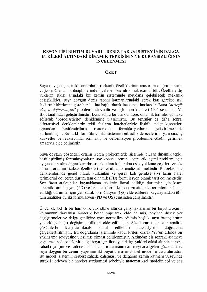
ÖZET
Suya doygun gözenekli ortamların mekanik özelliklerinin araştırılması, jeomekanik
ve jeo-mühendislik disiplinlerinde incelenen önemli konulardan biridir. Özellikle dış
yüklerin etkisi altındaki bir zemin sisteminde meydana gelebilecek mekanik
değişiklikler, suya doygun deniz tabanı katmanlarındaki gerek katı gerekse sıvı
fazların birbirlerine göre hareketine bağlı olarak incelenebilmektedir. Buna "birleşik
akış ve deformasyon" problemi adı verilir ve ilişkili denklemleri 1941 senesinde M.
Biot tarafından geliştirilmiştir. Daha sonra bu denklemlere, dinamik terimler de ilave
edilerek "poroelastisite" denklemine ulaşılmıştır. Bu terimler de daha sonra,
diferansiyel denklemlerde tekil fazların hareketleriyle ilişkili atalet kuvvetleri
açısından basitleştirilmiş matematik formülasyonların geliştirilmesinde
kullanılmıştır. Bu farklı formülasyonlar sistemin serbestlik derecelerinin yanı sıra; iç
kuvvetler ve reaksiyonlar için akış ve deformasyon problemine çözüm getirmek
amacıyla elde edilmiştir.
Suya doygun gözenekli ortamı içeren problemlerde sistemde oluşan dinamik tepki,
basitleştirilmiş formülasyonların söz konusu zemin - yapı etkileşimi problemi için
uygun olup olmadığını kararlaştırmak adına kullanılan esas yükleme çeşitleri ve söz
konusu ortamın fiziksel özellikleri temel alınarak analiz edilmektedir. Poroelastisite
denklemlerinde genel olarak kullanılan ve gerek katı gerekse sıvı fazın atalet
terimlerini de içeren durum tam dinamik (FD) formülasyon olarak tarif edilmektedir.
Sıvı fazın ataletinden kaynaklanan etkilerin ihmal edildiği durumlar için kısmi
dinamik formülasyon (PD) ve hem katı hem de sıvı faza ait atalet terimlerinin ihmal
edildiği durumlar için yarı statik formülasyon (QS) elde edilerek bu çalışmadaki tüm
tüm analizler bu iki formülasyon (PD ve QS) cinsinden çalışılmıştır.
Öncelikle belirli bir harmonik yük etkisi altında çalışmakta olan bir boyutlu zemin
kolonunun davranışı nümerik hesap yapılarak elde edilmiş, böylece düşey yer
değiştirmeler ve dalga genliğine göre normalize edilmiş boşluk suyu basınçlarının
yüksekliğe bağlı değişim grafikleri elde edilmiştir. Söz konusu sonuçlar analitik
çözümlerle karşılaştırılarak kabul edilebilir hassasiyette doğrulama
gerçekleştirilmiştir. Bu doğrulama işleminde kabul kriteri olarak %3‟ün altında bir
yakınsama seviyesine ulaşılmış olması belirlenmiştir. Ardından bir sonraki aşamaya
geçilerek, sadece tek bir dalga boyu için ilerleyen dalga yükleri etkisi altında serbest
sahada çalışan ve sadece tek bir zemin katmanından meydana gelen gözenekli ve
suya doygun bir zemin yapısının iki boyutlu matematiksel modeli oluşturulmuştur.
Bu model, sistemin serbest sahada çalışması ve dalganın zemin katmanı yüzeyinde
sürekli ilerleyen bir hareket sürdürmesi sebebiyle matematiksel modelin sol ve sağ
xxviii
tarafındaki sınır koşulları birbirine doğrusal bir fonksiyonla bağlı olacak şekilde tarif
edilerek sadece tek bir dalga boyu için hazırlanmıştır. Genel olarak bu çalışma
içerisindeki tüm matematiksel modellerde tanımlanan poroelastisite denklemlerinin
ayrıklaştırılması için klasik sonlu elemanlar yöntemi (FEM) kullanılması sebebiyle,
sonlu eleman parçalarının boyutlarında küçülmeye gidilerek bir kaç defa çözüm
gerçekleştirilmiş ve alınan sonuçların %3‟lük kabul edilebilir yakınsama derecesine
ulaşmasının ardından matematiksel modelleme kıstası belirlenmiştir. Bu işlemler
yapılırken de yine bir boyut için gerçekleştirilen çözümde de olduğu gibi nümerik
sonuçlar ile analitik sonuçlar; yakınsama kontrolleri, katı faz için elde edilen düşey
yer değiştirmeler, ilerleyen dalga genliğine göre normalize edilmiş boşluk suyu
basınçları ve efektif normal gerilmelerin derinliğe göre değişimi cinsinden
karşılaştırılmıştır. Sonuçlarda görülen kabul edilebilir yakınsama kriterinin
yakalanmasıyla birlikte harmonik duran dalga yüklerine maruz kalan bir keson tipi
rıhtım duvarı (CTQ) - deniz tabanı - dolgu zemin sisteminin dinamik tepkisi
değerlendirme işlemine geçilmiştir. Açık denizde ilerleyen dalganın rıhtım duvarı
yüzeyinden yansımasıyla birlikte ardındaki dalgalar ile girişimde bulunarak duran
dalga formuna dönüşmesi nedeniyle bu aşamada duran dalga etkisi dikkate
alınmıştır. Bu sistemin matematiksel modelinin temsil ettiği alanın genişliği, farklı
malzeme özelliklerine sahip çok sayıda katmanın bir arada kullanılması ve su
derinliğinin model içerisinde değişkenlik göstermesi sebebiyle elde edilen sonuçların
doğruluğunu kontrol edebilmek adına önceki bölümlerde de olduğu gibi sonlu
eleman parçalarının model alanı içerisindeki boyutu küçültülerek ve dolayısıyla
sayısı da kademeli olarak arttırılarak rıhtım duvarının ön topuk bölgesinden geçen
düşey doğrultudaki bir kesit üzerinden elde edilen sonuçlar karşılaştırılmış ve sistemi
en doğru şekilde temsil edecek sonlu eleman boyutları belirlenmiştir. Bununla
beraber, açık deniz etkisini de sisteme doğru bir şekilde tanımlayabilmek için de
matematiksel modelin açık denizi temsil eden düşey kenarının rıhtım duvarı ile
arasındaki mesafe kademeli olarak arttırılmış ve benzer şekilde en uygun açık deniz
mesafesi, duran dalga boyu cinsinden belirlenerek matematiksel modele aktarılmıştır.
Bu çalışmadaki temel odak noktası ağırlıklı olarak suya doygun gözenekli deniz
tabanının ve dolgunun etrafındaki toprağın dinamik tepkisinin özelliklerine ve
bunların duran dalga yükleri altındaki rıhtım duvarı duraysızlığına olan katkısıdır.
Çalışmada, Japonya'nın Kobe limanında bulunan ve 1995 yılındaki Hyogo-Ken
Nanbu depreminde önemli derecede hasar gören bir rıhtım duvarı - deniz tabanı -
dolgu sistemi dikkate alınmıştır. Bu analizler sırasında, hem PD hem de QS
formülasyonlarında, katı faz için zamansal ve mekansal alanlardaki düşey ve yatay
yer değiştirmeler, duran dalga genliğine göre normalize edilmiş boşluk suyu
basınçları ve kayma gerilmelerinin derinlikle değişim varyasyonları açısından sayısal
sonuçlar elde edilmiş ve karşılaştırılmalı olarak sunulmuştur.
CTQ – deniz tabanı sistemi ayrıca, zemindeki ani sıvılaşma potansiyeli göz önüne
alınarak duran dalga etkisi altında rıhtım duvarı duraysızlığı açısından da
değerlendirilmiştir. Bu analizler sırasında, sistemin dinamik tepkisinin araştırıldığı
bir önceki bölümden farklı olarak mevcut rıhtım duvarının, zemin katmanlarının ve
deniz suyunun kendi ağırlıklarından ötürü oluşan kuvvetler de matematiksel modele
aktarılmıştır. Neredeyse suya doygun deniz tabanı katmanında ve dolgu alanında
küçük hava boşlukları bulunduğunu varsayarak suya doygunluk derecesi deniz tabanı
için S=0.999 olacak şekilde tarif edilmiş, bu olgu sayısal olarak analiz edilmiş ve ani
sıvılaşma bölgeleri hesaplanan ortalama efektif gerilmenin sıfır veya pozitif
konturları cinsinden hesap alanı içerisinde tanımlanmıştır. Daha sonra duran dalga
xxix
yüksekliği sabit tutularak söz konusu sistem içerisinde sadece deniz tabanındaki
farklı geçirgenlik, zemin tipi ve açık denizde meydana gelen duran dalga periyodu
süresindeki (lineer dalga teorisine göre aynı zamanda dalga boyundaki) değişikliklere
göre sistemde oluşan dinamik tepkileri ve rıhtım duvarı duraysızlığı üzerindeki
etkileri belirlemek amacıyla bir takım parametrik çalışmalar yürütülmesinin ardından
her iki formülasyon (PD ve QS) için elde edilen sonuçlara ilişkin karşılaştırma
grafikleri sunulmuştur. Bununla beraber, bu çalışmanın geliştirilmesi için ileriki
zamanlarda yapılması düşünülen ve malzemenin doğrusal olmayan davranışlarının
da hesaba katılması ile birlikte sistemin gerçek tepkisine en yakın sonuçların elde
edilebilmesi adına ön bilgi oluşturabilecek şekilde kritik bölgelerin gösterilebildiği
kayma gerilmesi diyagramları da ayrıca gösterilmiştir. Sonuç olarak, deniz tabanı ve
dolgu toprağının ani sıvılaşma potansiyeline bakıldığında, söz konusu CTQ - deniz
tabanı sisteminin duran dalga etkisi altındaki dinamik tepkisi ve duraysızlığı
üzerinde, bu alanda çalışan kıyı ve jeoteknik tasarım mühendisleri ile diğer
araştırmacılar için yararlı olabileceği düşünülen sonuçlar elde edilmiştir.

xxx

1
1. INTRODUCTION
Today, the use of sea lanes has become very common both in terms of tourism as
well as in passenger transport and shipping for commerce. In this respect, a
significant budget is being spent to build ports worldwide. Therefore, coastal
protection measures are taken for all kinds of hazards that may arise from the sea and
constitute a physical threat to the port. Particularly, these measures are constructing
breakwaters along the coasts of communities and building quay walls along the
coastlines by harbor regions. The main task of these structures is to maintain stability
of coasts against severe wave actions. The idea here is to provide resistance to both
oscillatory and impact loads and other external disastrous effects such as ship strikes.
At the same time, they also provide security for structures on and around the ports.
Quay walls are marine structures that are built as a part of a port to sustain port‟s
integrity and provide protection. They are the most common types of construction for
docks because of their durability, ease of construction and capacity to reach deep
seabed levels. The design of gravity quay walls requires sufficient capacity for three
design criteria; sliding, overturning and allowable bearing capacity under the base of
the wall.
Until today, plenty of studies done by a large number of researchers is at a
satisfactory level to calculate the reaction they have given under static loads.
Unfortunately, since it is not possible to say the same thing under seismic loads,
therefore research studies on this subject are still conducted. In addition, because
these structures are directly connected to the sea, they have to be resistant not only to
structural loads, but also to wave loads. In the ocean, not only the impact of gigantic
waves called tsunamis generated mostly as a result of an an earthquake but waves
caused by large ship transits can also be quite challenging to incorporate their effects
on such protecting systems in these marine structures. In addition, the effects of these
2
waves on the soil layers lying under or at the back of the structures can also bring
about secondary problems.
There are several different ways to build these marine structures. Prefabricated and
L-shaped reinforced concrete structures on rubble fill, the caisson walls formed by
filling the reinforced concrete caisson with soil filling material, facing panels used
reinforcement bars to the walls of the anchorage technique and block walls which are
constructed by stacking reinforced concrete blocks are some of the current
construction techniques. The correct design of these marine structures is vital. As a
consequence of erroneous designs, for example, there may be problems such as wall
experiencing rocking motion that may cause collapse, excessive displacement,
breakage, cracking and insufficient resistance to wave loads to prevent the water
passage to seaport. However, the liquefaction that may occur in other soil layers in
the system to which the wall is attached is a serious hazard for structures located on
or near the shore. Unfortunately, it is not uncommon to see such failures among the
ports of the world coasts in this way.
While breakwaters are mainly used to protect the majority of a port against wave
action, it is safe to say that quay walls act as a secondary measure against coastal
hazards. Thus, it is also not a common practice to evaluate the dynamic response of
quay walls under severe wave conditions as more often than not it is breakwaters‟
job to protect such systems. However, sometimes that is not the case (i.e. the
Ambarli Port or the Asya Port in Turkey) and either there is no breakwater placed at
all or that quay wall acts as a protector while the breakwater is being built. Hence,
conducting such analyses for evaluating the quay wall response becomes a
requirement for us, researchers.
In the former, quay wall needs to be analyzed against severe wave action which is
the primary cause of instability while in the latter; the primary cause of instability
becomes the earthquake excitation. Today, it is possible to see that many researchers
focus on damages experienced by such systems that can occur under earthquake
loads. However, it is not correct to just ascertain such dynamic effects exclusively
3
through earthquake loads. A coastal structure that has not been damaged by
earthquakes or has not been subjected to any previous seismic shaking can suffer
severe damage under the influence of progressive or standing waves. Surprisingly,
just few studies that consider waves as the major cause of failure are made by the
researchers. In these studies, a gravity type quay wall containing several layers of
concrete blocks with a special cross section is generally analyzed under standing
wave effects. On the other hand, in the coastal areas prone to earthquakes, it is
absolutely necessary to examine the dynamic response of the CTQ. For this purpose,
various researchers have worked on such coastal structures which are mentioned
below in the brief literature survey.
It has been common to examine the response of coastal structures under various
types of waves using numerical models frequently used in the solution of geo-
engineering problems. With the increased use of computers and the help of advanced
softwares, finite element (FE) models are created and thus, more accurate results are
achieved.
In this study, following the development of the FE model which models the system
in question, parametric studies are carried out using different soil types, wave periods
and permeability coefficients. The time required for the system to reach steady state
during loading is taken into account. Then, standing wave-induced pore water
pressures, solid soil displacements, shear stresses are evaluated and the instantaneous
liquefaction potential of a real CTQ-rubble-seabed system damaged in the 1995
Hyogoken-Nanbu earthquake in Port Island is computed through classical finite
element analyses.

4
5
2. LITERATURE REVIEW
2.1 Quay Walls as Marine Structures
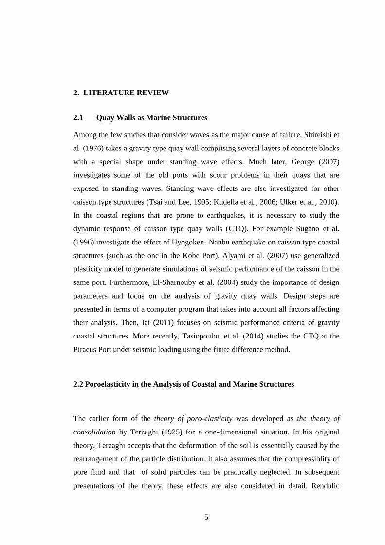
Among the few studies that consider waves as the major cause of failure, Shireishi et
al. (1976) takes a gravity type quay wall comprising several layers of concrete blocks
with a special shape under standing wave effects. Much later, George (2007)
investigates some of the old ports with scour problems in their quays that are
exposed to standing waves. Standing wave effects are also investigated for other
caisson type structures (Tsai and Lee, 1995; Kudella et al., 2006; Ulker et al., 2010).
In the coastal regions that are prone to earthquakes, it is necessary to study the
dynamic response of caisson type quay walls (CTQ). For example Sugano et al.
(1996) investigate the effect of Hyogoken- Nanbu earthquake on caisson type coastal
structures (such as the one in the Kobe Port). Alyami et al. (2007) use generalized
plasticity model to generate simulations of seismic performance of the caisson in the
same port. Furthermore, El-Sharnouby et al. (2004) study the importance of design
parameters and focus on the analysis of gravity quay walls. Design steps are
presented in terms of a computer program that takes into account all factors affecting
their analysis. Then, Iai (2011) focuses on seismic performance criteria of gravity
coastal structures. More recently, Tasiopoulou et al. (2014) studies the CTQ at the
Piraeus Port under seismic loading using the finite difference method.
2.2 Poroelasticity in the Analysis of Coastal and Marine Structures
The earlier form of the theory of poro-elasticity was developed as the theory of
consolidation by Terzaghi (1925) for a one-dimensional situation. In his original
theory, Terzaghi accepts that the deformation of the soil is essentially caused by the
rearrangement of the particle distribution. It also assumes that the compressiblity of
pore fluid and that of solid particles can be practically neglected. In subsequent
presentations of the theory, these effects are also considered in detail. Rendulic
6
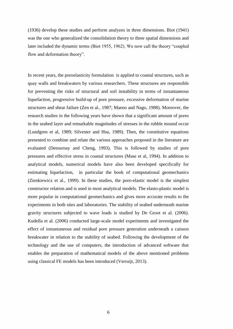
(1936) develop these studies and perform analyzes in three dimensions. Biot (1941)
was the one who generalized the consolidation theory to three spatial dimensions and
later included the dynamic terms (Biot 1955, 1962). We now call the theory “coupled
flow and deformation theory”.
In recent years, the poroelasticity formulation is applied to coastal structures, such as
quay walls and breakwaters by various researchers. These structures are responsible
for preventing the risks of structural and soil instability in terms of instantaneous
liquefaction, progressive build-up of pore pressure, excessive deformation of marine
structures and shear failure (Zen et al., 1987; Maeno and Nago, 1988). Moreover, the
research studies in the following years have shown that a significant amount of pores
in the seabed layer and remarkable magnitudes of stresses in the rubble mound occur
(Lundgren et al, 1989; Silvester and Hsu, 1989). Then, the constitutive equations
presented to combine and relate the various approaches proposed in the literature are
evaluated (Detournay and Cheng, 1993). This is followed by studies of pore
pressures and effective stress in coastal structures (Mase et al, 1994). In addition to
analytical models, numerical models have also been developed specifically for
estimating liquefaction, in particular the book of computational geomechanics
(Zienkiewicz et al., 1999). In these studies, the poro-elastic model is the simplest
constructor relation and is used in most analytical models. The elasto-plastic model is
more popular in computational geomechanics and gives more accurate results to the
experiments in both sites and laboratories. The stability of seabed underneath marine
gravity structures subjected to wave loads is studied by De Groot et al. (2006).
Kudella et al. (2006) conducted large-scale model experiments and investigated the
effect of instantaneous and residual pore pressure generation underneath a caisson
breakwater in relation to the stability of seabed. Following the development of the
technology and the use of computers, the introduction of advanced software that
enables the preparation of mathematical models of the above mentioned problems
using classical FE models has been introduced (Verruijt, 2013).

7
2.3 Liquefaction Studies
In the analysis of the liquefaction potential in the field, "Simplified Liquefaction
Analysis" is widely used at earlier times (Seed and Idriss, 1971). The liquefaction
resistance of soil layers is often correlated with the results of field trials. Although
seabed liquefaction under progressive waves has been extensively investigated, only
a few works have been done on the liquefaction of seabed under standing waves.
Sekiguchi et al. (1995) used a centrifugal wave test to obtain some useful
experimental data. The test set-up by Sassa and Sekiguchi (1999) was designed to
measure pore pressures that indicated that the antinodal section was where the
liquefaction was observed, although the soil did not encounter any shear stresses in
the section. Other study results show that the residual liquefaction causes that blocks
on marine structures sink in such a liquefied soil as a result of their own weight
(Suzuki et al., 1998; Sumer et al., 1999). The latter study examines the damage
caused on coastal structures as a result of wave-induced liquefaction and associated
drifting movement (Kirca, 2013).
In addition, instantaneous liquefaction studies have been the center of attention for
researchers, in the last couple of decades. This mechanism occurs in a seabed having
some air in the voids. Therefore; the major cause of sinking of breakwaters is
investigated in terms of instantansoue liquefaction (Sakai et al., 1995; Sumer and
Fredsøe, 2002; Ulker et al., 2010; Ulker et al., 2012; Ulker 2012). Moreover, studies
on tsunami scour and sedimentation have been carried out with the potential for
instantaneous liquefaction (Yeh and Li, 2008). Then, in a comprehensive study on
instantaneous liquefaction, analytical solutions and numerical models are developed
for the response of plane strain saturated porous media, and wave-induced response
of seabed in free field and around a breakwater under pulsating/breaking waves are
investigated (Ulker, 2009). Recently, the effect of degree of saturation on
instantaneous liquefaction of seabed around a rubble mound breakwater is presented
by (Ulker and Massah Fard, 2016).

8
9
3. MATHEMATICAL FORMULATION OF POROELASTICITY:
DYNAMICS OF SATURATED POROUS SEABED
It is generally undesirable to describe soils as solid materials in geomechanics. Soils
are composed of varying size and shape of solid particles, and often the pore space
between these particles is filled with a fluid (generally water). This multi-phase
structure is called “saturated or partially saturated porous media” in soil mechanics.
The deformation of this porous medium depends on the rigidity of the porous
material and the flow of the fluid in the pores. If the permeability of the material is
negligibly small, rate of deformations decrease due to partly the viscous actions of
the fluid in the pores but mostly due to reduction of the ability for flow to take place
through the small size pores. The simultaneous deformation of a porous medium and
the flow of pore fluid is the main subject matter in geomechanics. Therefore, it is
necessary to analyze the soil response under external loads by using the equations
governing the actual behavior as observed in nature. These equations are derived
considering three basic physical laws namely;
1. Constitutive law
2. Law of conservation of momentum
3. Law of conservation of mass
These laws result in;
The stress-strain relationship
The momentum balance (i.e. equilibrium equations)
The mass balance equation, (i.e. continuity equation)
respectively.
10
3.1 Governing Equations
Saturated poromechanics is described as the „theory of coupled flow and
deformation‟ developed first by Biot (1941, 1955 and 1962) which is also known as
the theory of dynamic consolidation as indicated before. Principle of effective stress,
as introduced by Terzaghi (1925), is defined as the stress developed as the average of
contact stresses along a cross section in the soil skeleton. In developing a general
mathematical formulation governing the behavior of this two-phase soil field, the
following assumptions are made:
(1) The water and the gas phases within the porous medium are considered as a
single compressible fluid.
(2) The effect of gas diffusing through water and movement of water vapor is
neglected.
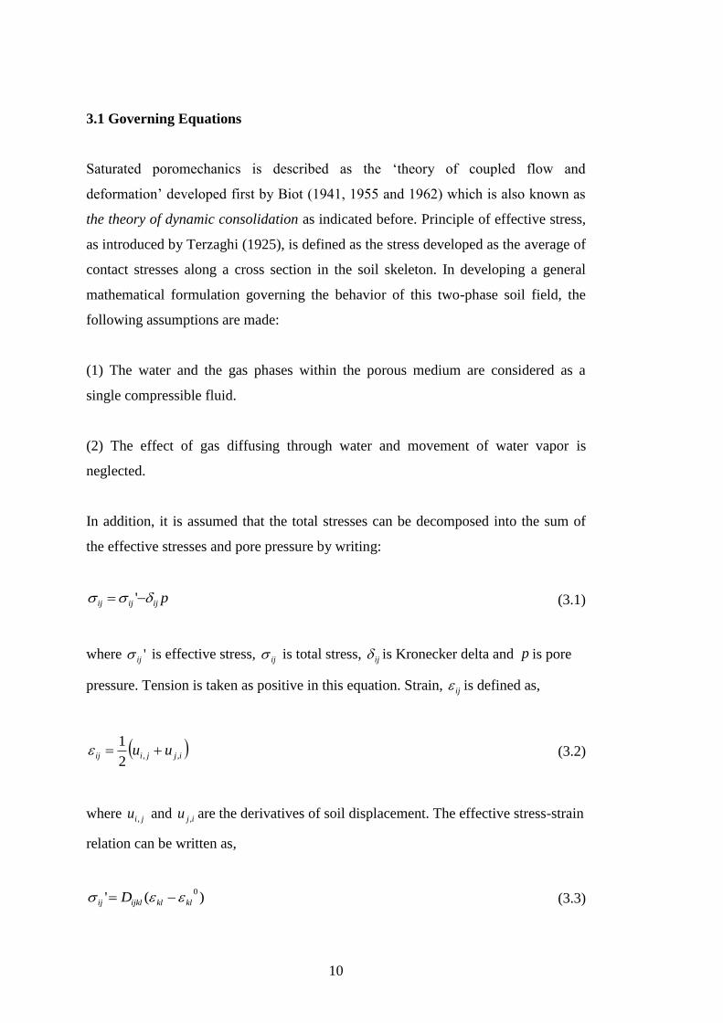
In addition, it is assumed that the total stresses can be decomposed into the sum of
the effective stresses and pore pressure by writing:
(3.1)
where is effective stress, is total stress, is Kronecker delta and is pore
pressure. Tension is taken as positive in this equation. Strain, is defined as,
(3.2)
where and are the derivatives of soil displacement. The effective stress-strain
relation can be written as,
(3.3)
pijijij '
'ij ij ij p
ij
ijjiij uu ,,
2
1
jiu , iju ,
)('0
klklijklij D
11
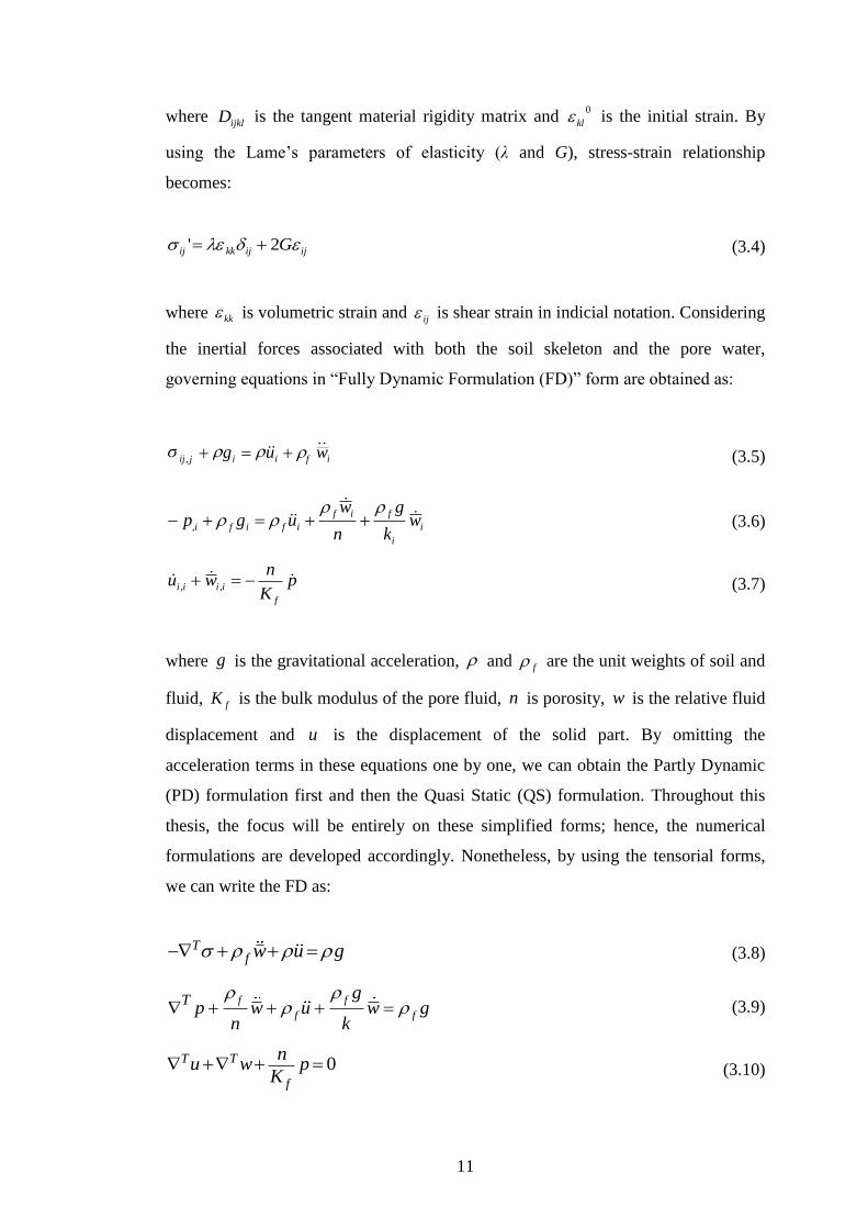
where is the tangent material rigidity matrix and is the initial strain. By
using the Lame‟s parameters of elasticity (λ and G), stress-strain relationship
becomes:
(3.4)
where is volumetric strain and is shear strain in indicial notation. Considering
the inertial forces associated with both the soil skeleton and the pore water,
governing equations in “Fully Dynamic Formulation (FD)” form are obtained as:
(3.5)
(3.6)
(3.7)
where is the gravitational acceleration, and are the unit weights of soil and
fluid, is the bulk modulus of the pore fluid, is porosity, is the relative fluid
displacement and is the displacement of the solid part. By omitting the
acceleration terms in these equations one by one, we can obtain the Partly Dynamic
(PD) formulation first and then the Quasi Static (QS) formulation. Throughout this
thesis, the focus will be entirely on these simplified forms; hence, the numerical
formulations are developed accordingly. Nonetheless, by using the tensorial forms,
we can write the FD as:
(3.8)
(3.9)
(3.10)
ijklD0
kl
ijijkkij G 2'
kkij
i
i
fif
ififi wk
g
n
wugp
,
pK
nwu
f
iiii ,,
g f
fK n w
u
Tf w u g
f f
f f
T gp w u w g
n k
0T T
f
nu w p
K
i f i i j ij w u g ,
12
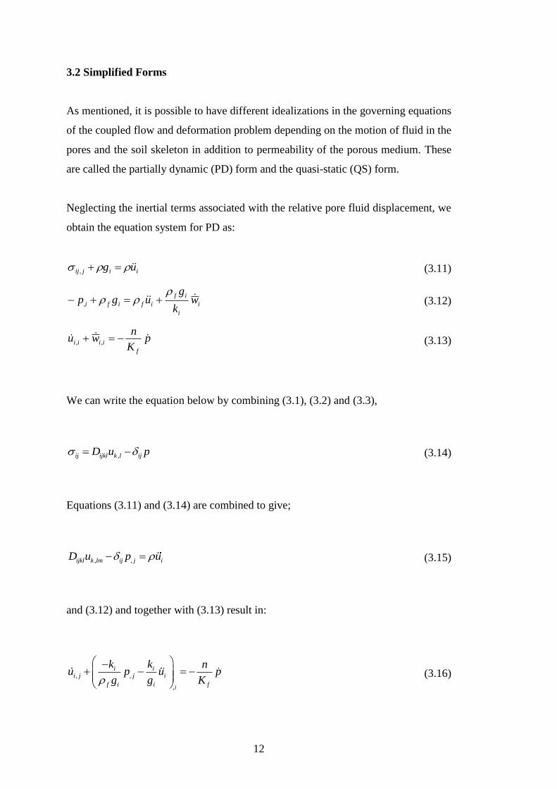
3.2 Simplified Forms
As mentioned, it is possible to have different idealizations in the governing equations
of the coupled flow and deformation problem depending on the motion of fluid in the
pores and the soil skeleton in addition to permeability of the porous medium. These
are called the partially dynamic (PD) form and the quasi-static (QS) form.
Neglecting the inertial terms associated with the relative pore fluid displacement, we
obtain the equation system for PD as:
(3.11)
(3.12)
(3.13)
We can write the equation below by combining (3.1), (3.2) and (3.3),
,ij ijkl k l ijD u p (3.14)
Equations (3.11) and (3.14) are combined to give;
, ,ijkl k lm ij j iD u p u (3.15)
and (3.12) and together with (3.13) result in:
, ,
,
i ii j j i
f i i fi
k k nu p u p
g g K
(3.16)
iijij ug ,
i
i
if
ififi wk
gugp
,
pK
nwu
f
iiii ,,
13
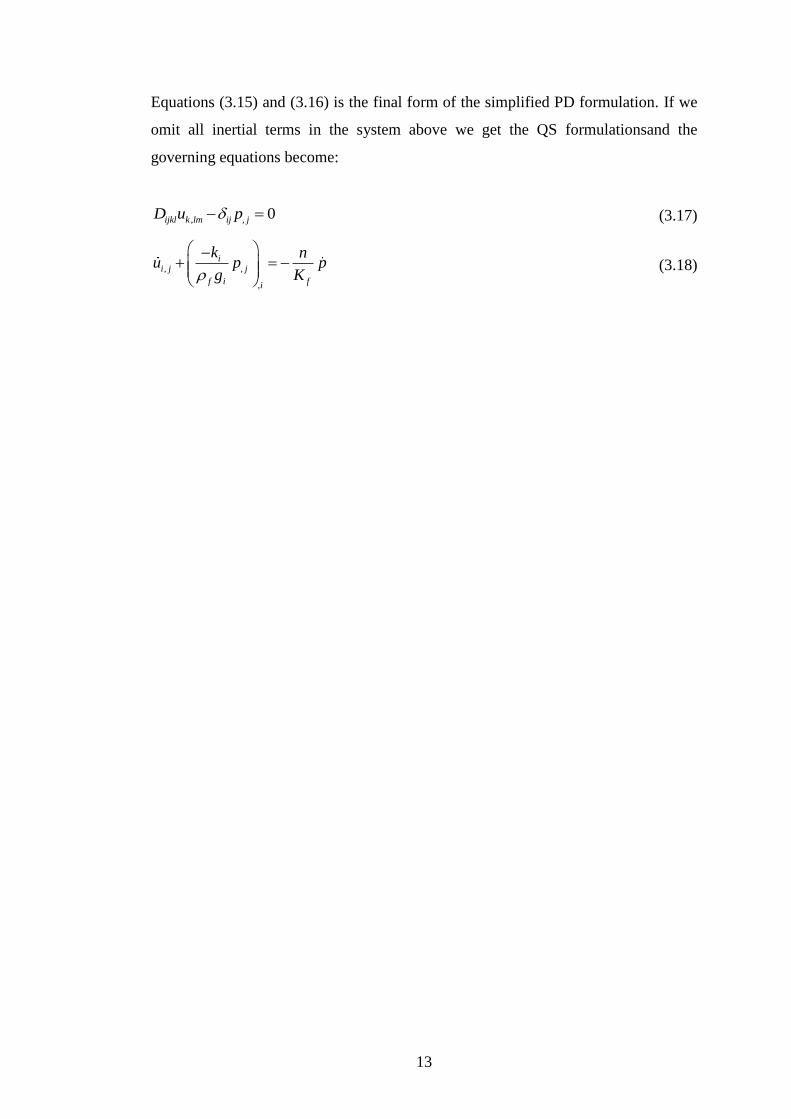
Equations (3.15) and (3.16) is the final form of the simplified PD formulation. If we
omit all inertial terms in the system above we get the QS formulationsand the
governing equations become:
, , 0ijkl k lm ij jD u p (3.17)
, ,
,
ii j j
f i fi
k nu p p
g K
(3.18)

14
15
4. NUMERICAL FORMULATION
As in many engineering branches, it is difficult to describe a problem in geo-
engineering as close to the actual behavior observed in real life as possible and to
determine the natural behavior of engineering systems under dynamic loads. Solving
these difficult problems with the available scientific methods is possible exclusively
through numerical methods implemented in computers that can do many operations
simultaneously in a short amount of time. For that, we need numerical methods to
solve a series of algebraic linear (or nonlinear) system of equations gathered from
actual governing partial differential equations of the physical system. In this thesis,
the classical finite element method (FEM) is used to discretize the governing
equations of poroelasticity as was presented in the previous chapter. Below presents
a summary of the FE formulations in Ulker (2009) and used here.
4.1 Finite Element Formulations
The necessary FE formulation is derived based on the “principal of virtual work”
written in terms of weak formulation of the governing equations followed by the FE
approximation of field variables and their time derivatives within the domain of
interest.
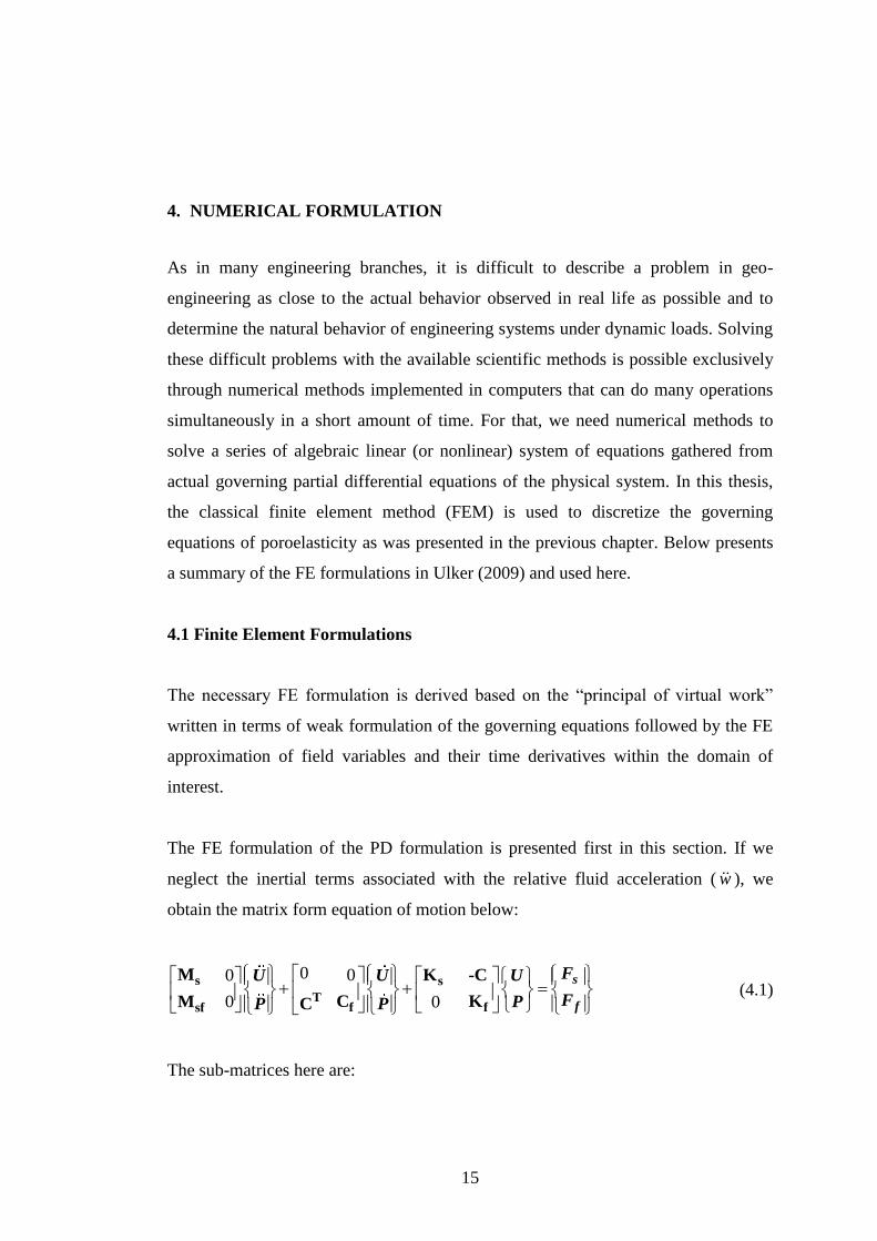
The FE formulation of the PD formulation is presented first in this section. If we
neglect the inertial terms associated with the relative fluid acceleration ( w ), we
obtain the matrix form equation of motion below:
0 00
0 0
s s
Tf fsf
M K -C
C KM C
s
f
FU U U
FPP P (4.1)
The sub-matrices here are:
16
T
u uB D B d
sK
(4.2)
T
p pf
kB B d
g
fK
(4.3)
T
u pB m N d
C
(4.4)
T
p pf
nN N d
K
fC
(4.5)
T
u uN N d
sM
(4.6)
T
p u
kB N d
g
sfM
(4.7)
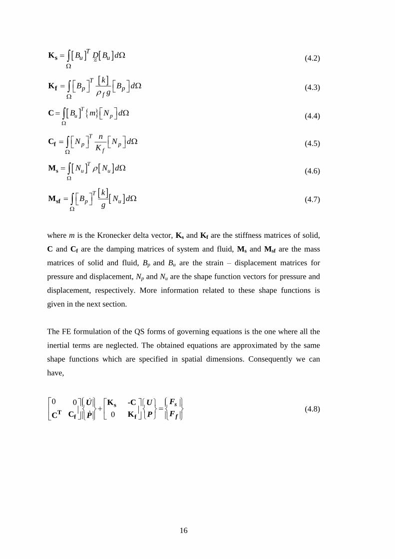
where m is the Kronecker delta vector, Ks and Kf are the stiffness matrices of solid,
C and Cf are the damping matrices of system and fluid, Ms and Msf are the mass
matrices of solid and fluid, Bp and Bu are the strain – displacement matrices for
pressure and displacement, Np and Nu are the shape function vectors for pressure and
displacement, respectively. More information related to these shape functions is
given in the next section.
The FE formulation of the QS forms of governing equations is the one where all the
inertial terms are neglected. The obtained equations are approximated by the same
shape functions which are specified in spatial dimensions. Consequently we can
have,
0 0
0
s
Tf f
K -C
C KC
s
f
FU U
FPP
(4.8)
17
5. FINITE ELEMENT ANALYSES: DETAILS
5.1 Spatial Integration
5.1.1 Gauss quadrature
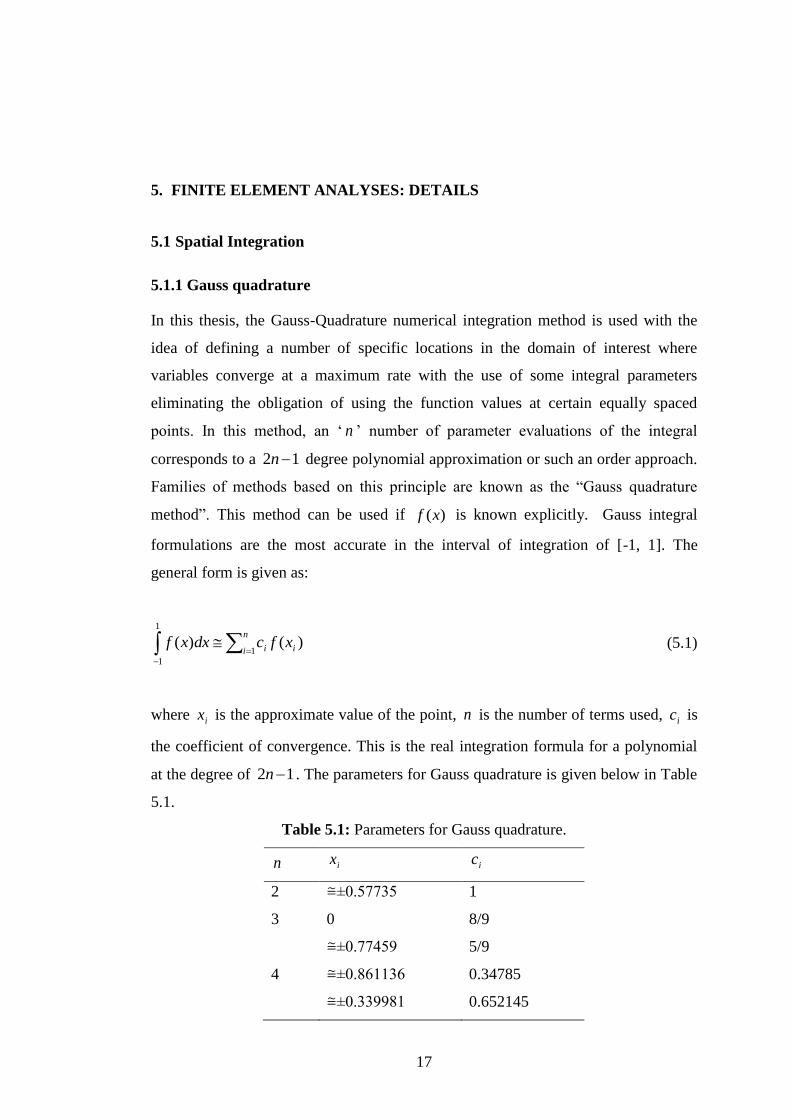
In this thesis, the Gauss-Quadrature numerical integration method is used with the
idea of defining a number of specific locations in the domain of interest where
variables converge at a maximum rate with the use of some integral parameters
eliminating the obligation of using the function values at certain equally spaced
points. In this method, an „ n ‟ number of parameter evaluations of the integral
corresponds to a 12 n degree polynomial approximation or such an order approach.
Families of methods based on this principle are known as the “Gauss quadrature
method”. This method can be used if )(xf is known explicitly. Gauss integral
formulations are the most accurate in the interval of integration of [-1, 1]. The
general form is given as:
1
11
)()(n
i ii xfcdxxf (5.1)
where ix is the approximate value of the point, n is the number of terms used, ic is
the coefficient of convergence. This is the real integration formula for a polynomial
at the degree of 12 n . The parameters for Gauss quadrature is given below in Table
5.1.
Table 5.1: Parameters for Gauss quadrature.
n ix ic
2 ±0.57735 1
3 0 8/9
±0.77459 5/9
4 ±0.861136 0.34785
±0.339981 0.652145
18
5.1.2 Shape functions
The element types are called as Constant Strain Triangle (CST), Linear Strain
Triangle (LST), Linear Quadrilateral (Q4), and Quadratic Quadrilateral (Q8). CST
and Q4 are usually used together in a mesh with linear elements. LST and Q8 are
generally applied in a mesh composed of quadratic elements. Quadratic elements are
preferred for stress analysis because of their high accuracy and the flexibility in
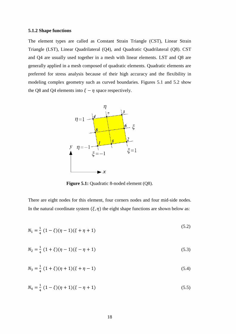
modeling complex geometry such as curved boundaries. Figures 5.1 and 5.2 show
the Q8 and Q4 elements into space respectively.
Figure 5.1: Quadratic 8-noded element (Q8).
There are eight nodes for this element, four corners nodes and four mid‐side nodes.
In the natural coordinate system the eight shape functions are shown below as:
(5.2)
(5.3)
(5.4)
(5.5)
19
(5.6)
(5.7)
(5.8)
(5.9)
We have ∑ at any point inside the element. The displacement field is
given by
[∑ ] (5.10)
[∑ ] (5.11)
which are quadratic functions over the element. Strains and stresses over a quadratic
quadrilateral element are quadratic functions, which are better representations.
The Q8 elements for the u-field integration are generally preferred because of more
accurate modeling of shear and volumetric deformations of the soil and due to spatial
convergence.
The shape functions used for the pressure are preferred as having one order of
polynomial degree less than they are for the displacement DOF, since the rate of
convergence of the pressure is greater than the rate of convergence of the
displacement. Thus, Q8 shape functions for the u-field and Q4 shape functions for
the p-field are used in the finite element analyses. The shape functions for Q4 are
shown below:
(5.12)
20
(5.13)
(5.14)
(5.15)
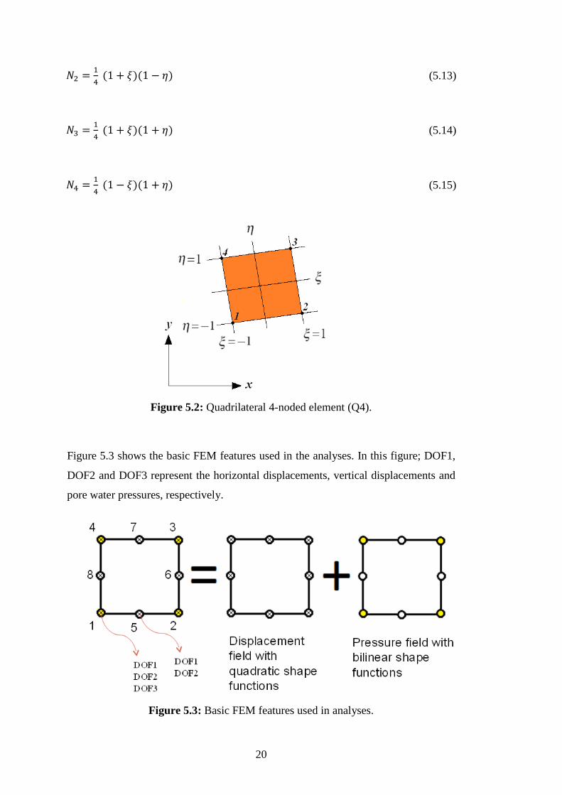
Figure 5.2: Quadrilateral 4-noded element (Q4).
Figure 5.3 shows the basic FEM features used in the analyses. In this figure; DOF1,
DOF2 and DOF3 represent the horizontal displacements, vertical displacements and
pore water pressures, respectively.
Figure 5.3: Basic FEM features used in analyses.

21
5.2 Temporal Integration
5.2.1 Implicit Newmark-β method
Time integration for obtaining the numerical results is carried out by using the
Implicit Newmark-β Method. So, at time step n+1, we have,
1 1 1 1n n n nMX CX KX R (5.16)
For the X vector, the relations for the acceleration, velocity and the displacement are,
1 1n n nX X X (5.17)
1 11n n n nX X t X X (5.18)
2
1 11 2 22
n n n n n
tX X tX X X
(5.19)
Here, and are the Newmark parameters controlling the stability and convergence
of the numerical solution that have a certain range of values to be able to obtain
unconditional stability with certain accuracy. The second order accuracy is attained
for numerically undamped scheme if =0.5 and =0.25. Conversely, if numerical
damping is desired, then the accuracy declines to first order. By solving (5.15) for
1nX , then substituting it into (5.14), we get
nnnnn XXtXXt
X
1
2
11121
(5.20)
nnnnn XtXXXt
X
1
2111
(5.21)
These equations are substituted into (5.12) and then are solved for 1nX . It becomes,
22
12 2
1
1 1 1 11
2
1 12
n n n n
n n n n
M C K X M X X Xt t t t
C X X t X Rt
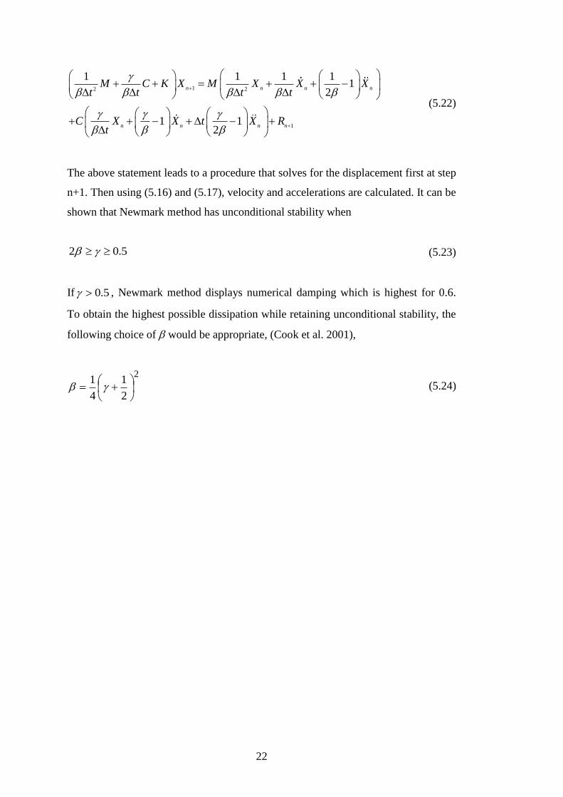
(5.22)
The above statement leads to a procedure that solves for the displacement first at step
n+1. Then using (5.16) and (5.17), velocity and accelerations are calculated. It can be
shown that Newmark method has unconditional stability when
5.02 (5.23)
If 5.0 , Newmark method displays numerical damping which is highest for 0.6.
To obtain the highest possible dissipation while retaining unconditional stability, the
following choice of would be appropriate, (Cook et al. 2001),
2
2
1
4
1
(5.24)
23
6. VERIFICATION ANALYSES
The main purpose of this chapter is that the mathematical formulations presented in
Chapter 4 are implemented in a computer program developed by (Guddati et al.,
2009) and requires verification by solving a number of basic problems in the free
field where there is no coastal structure in the vicinity, which have their analytical
solutions readily available. So, two problems with soil layers in 1-D and 2-D are
picked along with their analytical solutions developed by Ulker (2009). The idea
behind this is that possible FE results matching with their analytical counterparts
provide confidence in both the mathematics of the formulation and their
implementation into a computer as a code.
6.1 Problem 1: One-Dimensional Soil Column Response under Cyclic Wave
6.1.1 Problem definition
In this section the general analytical solutions for 1-D response are presented. The
solution is developed for a soil column that refers a porous media under cyclic wave
loading for PD formulations. The input data for soil material and the numerical
values of the other parameters used in 1-D analysis are presented in Table 6.1. Figure
6.1 presents the 1-D seabed soil under cyclic wave loading. The cyclic wave induced
pressures and forces are applied in terms of time histories evaluated from the
equation below:
).cos(0, iji tqq (6.1)
where jiq , is the pressure, 0q is the wave amplitude and is the wave angular
frequency.
24
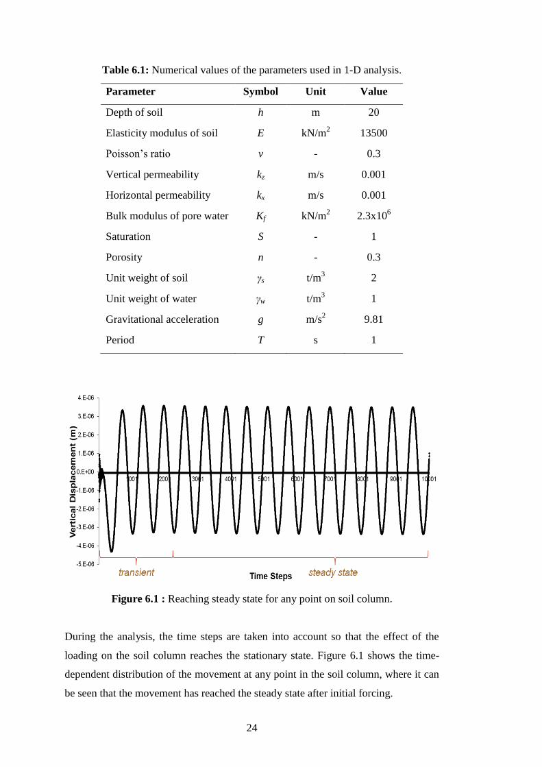
Table 6.1: Numerical values of the parameters used in 1-D analysis.
Parameter Symbol Unit Value
Depth of soil h m 20
Elasticity modulus of soil E kN/m2 13500
Poisson‟s ratio v - 0.3
Vertical permeability kz m/s 0.001
Horizontal permeability kx m/s 0.001
Bulk modulus of pore water Kf kN/m2 2.3x10
6
Saturation S - 1
Porosity n - 0.3
Unit weight of soil γs t/m3 2
Unit weight of water γw t/m3 1
Gravitational acceleration g m/s2 9.81
Period T s 1
Figure 6.1 : Reaching steady state for any point on soil column.
During the analysis, the time steps are taken into account so that the effect of the
loading on the soil column reaches the stationary state. Figure 6.1 shows the time-
dependent distribution of the movement at any point in the soil column, where it can
be seen that the movement has reached the steady state after initial forcing.
25
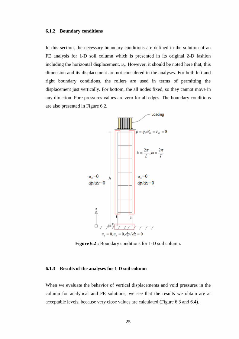
6.1.2 Boundary conditions
In this section, the necessary boundary conditions are defined in the solution of an
FE analysis for 1-D soil column which is presented in its original 2-D fashion
including the horizontal displacement, ux. However, it should be noted here that, this
dimension and its displacement are not considered in the analyses. For both left and
right boundary conditions, the rollers are used in terms of permitting the
displacement just vertically. For bottom, the all nodes fixed, so they cannot move in
any direction. Pore pressures values are zero for all edges. The boundary conditions
are also presented in Figure 6.2.
Figure 6.2 : Boundary conditions for 1-D soil column.
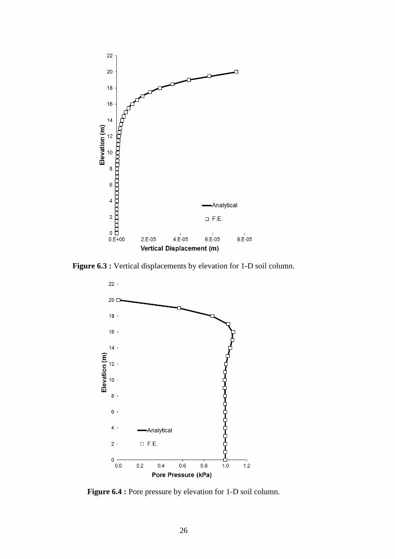
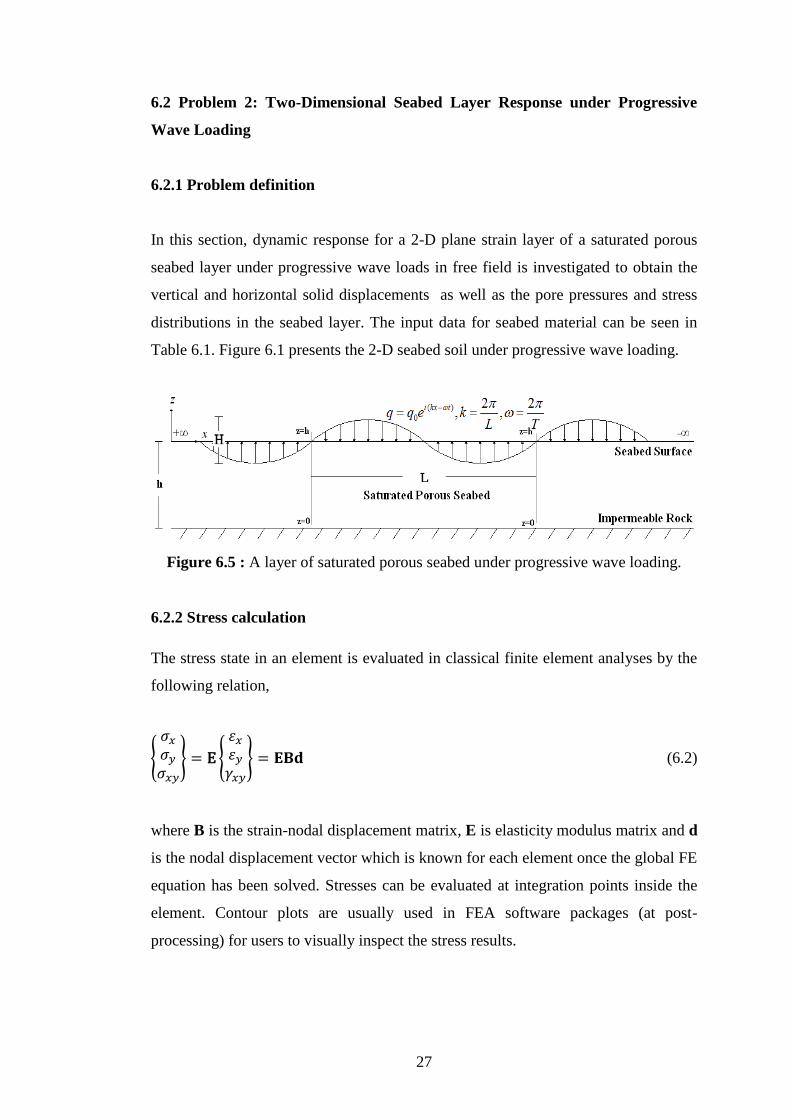
6.1.3 Results of the analyses for 1-D soil column
When we evaluate the behavior of vertical displacements and void pressures in the
column for analytical and FE solutions, we see that the results we obtain are at
acceptable levels, because very close values are calculated (Figure 6.3 and 6.4).
26
Figure 6.3 : Vertical displacements by elevation for 1-D soil column.
Figure 6.4 : Pore pressure by elevation for 1-D soil column.
27
6.2 Problem 2: Two-Dimensional Seabed Layer Response under Progressive
Wave Loading
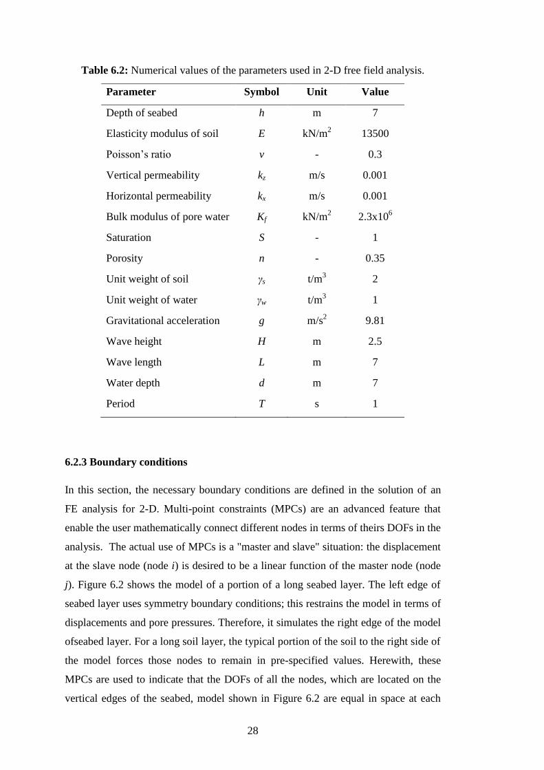
6.2.1 Problem definition
In this section, dynamic response for a 2-D plane strain layer of a saturated porous
seabed layer under progressive wave loads in free field is investigated to obtain the
vertical and horizontal solid displacements as well as the pore pressures and stress
distributions in the seabed layer. The input data for seabed material can be seen in
Table 6.1. Figure 6.1 presents the 2-D seabed soil under progressive wave loading.
Figure 6.5 : A layer of saturated porous seabed under progressive wave loading.
6.2.2 Stress calculation
The stress state in an element is evaluated in classical finite element analyses by the
following relation,
{
} {
} (6.2)
where B is the strain-nodal displacement matrix, E is elasticity modulus matrix and d
is the nodal displacement vector which is known for each element once the global FE
equation has been solved. Stresses can be evaluated at integration points inside the
element. Contour plots are usually used in FEA software packages (at post-
processing) for users to visually inspect the stress results.
28
Table 6.2: Numerical values of the parameters used in 2-D free field analysis.
Parameter Symbol Unit Value
Depth of seabed h m 7
Elasticity modulus of soil E kN/m2 13500
Poisson‟s ratio v - 0.3
Vertical permeability kz m/s 0.001
Horizontal permeability kx m/s 0.001
Bulk modulus of pore water Kf kN/m2 2.3x10
6
Saturation S - 1
Porosity n - 0.35
Unit weight of soil γs t/m3 2
Unit weight of water γw t/m3 1
Gravitational acceleration g m/s2 9.81
Wave height H m 2.5
Wave length L m 7
Water depth d m 7
Period T s 1
6.2.3 Boundary conditions
In this section, the necessary boundary conditions are defined in the solution of an
FE analysis for 2-D. Multi-point constraints (MPCs) are an advanced feature that
enable the user mathematically connect different nodes in terms of theirs DOFs in the
analysis. The actual use of MPCs is a "master and slave" situation: the displacement
at the slave node (node i) is desired to be a linear function of the master node (node
j). Figure 6.2 shows the model of a portion of a long seabed layer. The left edge of
seabed layer uses symmetry boundary conditions; this restrains the model in terms of
displacements and pore pressures. Therefore, it simulates the right edge of the model
ofseabed layer. For a long soil layer, the typical portion of the soil to the right side of
the model forces those nodes to remain in pre-specified values. Herewith, these
MPCs are used to indicate that the DOFs of all the nodes, which are located on the
vertical edges of the seabed, model shown in Figure 6.2 are equal in space at each
29
time step. In addition, with this feature, it is possible to calculate the wave effect of
the whole seabed system by modeling for only a single wavelength of the progressive
wave.
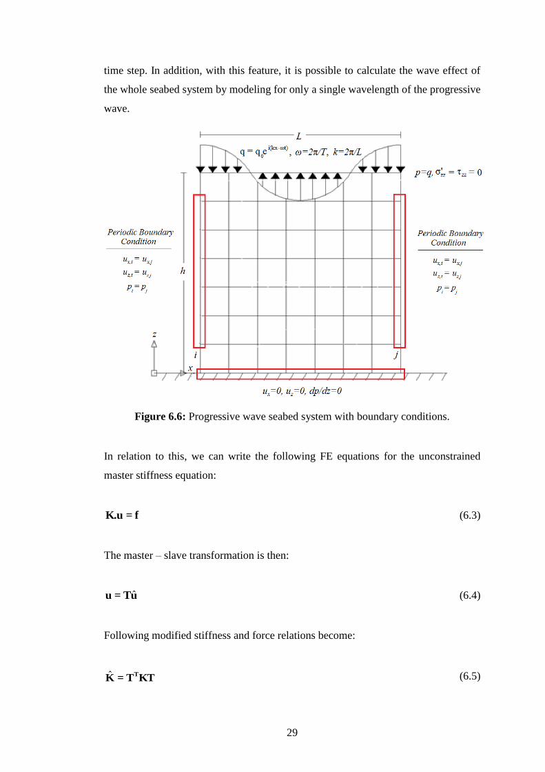
Figure 6.6: Progressive wave seabed system with boundary conditions.
In relation to this, we can write the following FE equations for the unconstrained
master stiffness equation:
f=K.u (6.3)
The master – slave transformation is then:
uT=u ˆ (6.4)
Following modified stiffness and force relations become:
KTT=KTˆ (6.5)
30
fT=fTˆ (6.6)
where K is stiffness matrix, u is displacement matrix, f is force matrix, T is
transformation matrix, K is modified stiffness matrix, f is modified force matrix, u
is modified displacement matrix. As a final point the modified stiffness equation is
obtained as:
f=uKˆˆ (6.7)
The DOFs are classified into three types: independent or uncommitted, masters and
slaves. Including these DOFs, equation (5.6) can be rewritten as:
[
] [
] [
] (6.8)
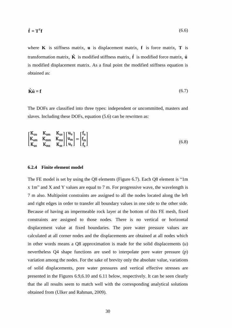
6.2.4 Finite element model
The FE model is set by using the Q8 elements (Figure 6.7). Each Q8 element is “1m
x 1m” and X and Y values are equal to 7 m. For progressive wave, the wavelength is
7 m also. Multipoint constraints are assigned to all the nodes located along the left
and right edges in order to transfer all boundary values in one side to the other side.
Because of having an impermeable rock layer at the bottom of this FE mesh, fixed
constraints are assigned to those nodes. There is no vertical or horizontal
displacement value at fixed boundaries. The pore water pressure values are
calculated at all corner nodes and the displacements are obtained at all nodes which
in other words means a Q8 approximation is made for the solid displacements (u)
nevertheless Q4 shape functions are used to interpolate pore water pressure (p)
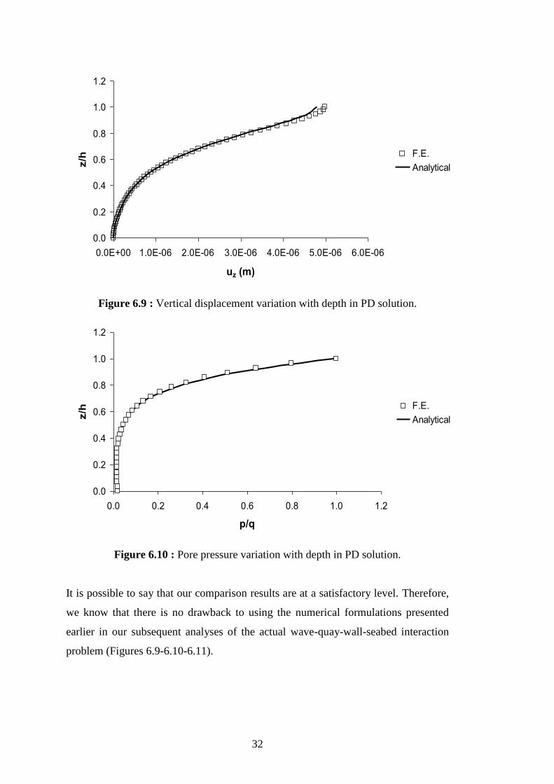
variation among the nodes. For the sake of brevity only the absolute value, variations
of solid displacements, pore water pressures and vertical effective stresses are
presented in the Figures 6.9,6.10 and 6.11 below, respectively. It can be seen clearly
that the all results seem to match well with the corresponding analytical solutions
obtained from (Ulker and Rahman, 2009).
31
Figure 6.7 : FE mesh.
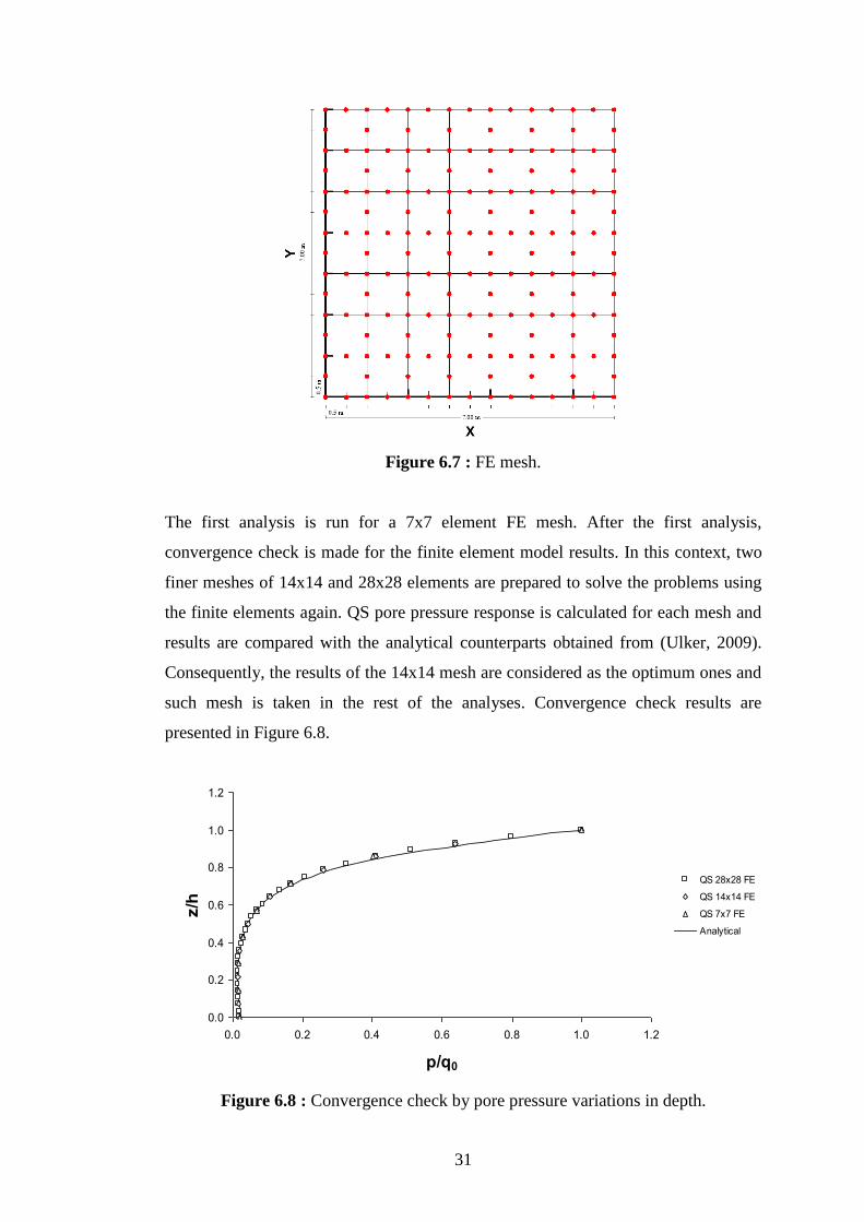
The first analysis is run for a 7x7 element FE mesh. After the first analysis,
convergence check is made for the finite element model results. In this context, two
finer meshes of 14x14 and 28x28 elements are prepared to solve the problems using
the finite elements again. QS pore pressure response is calculated for each mesh and
results are compared with the analytical counterparts obtained from (Ulker, 2009).
Consequently, the results of the 14x14 mesh are considered as the optimum ones and
such mesh is taken in the rest of the analyses. Convergence check results are
presented in Figure 6.8.
Figure 6.8 : Convergence check by pore pressure variations in depth.
0.0
0.2
0.4
0.6
0.8
1.0
1.2
0.0 0.2 0.4 0.6 0.8 1.0 1.2
p/q0
z/h
QS 28x28 FE
QS 14x14 FE
QS 7x7 FE
Analytical
32
Figure 6.9 : Vertical displacement variation with depth in PD solution.
Figure 6.10 : Pore pressure variation with depth in PD solution.
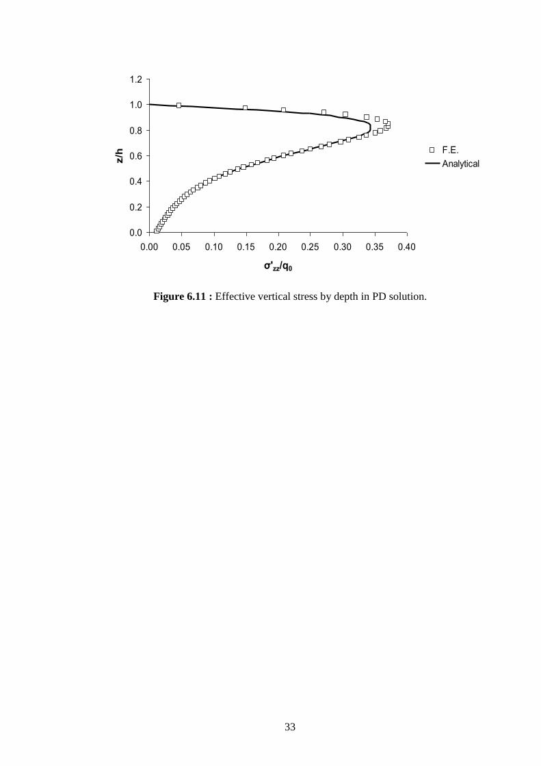
It is possible to say that our comparison results are at a satisfactory level. Therefore,
we know that there is no drawback to using the numerical formulations presented
earlier in our subsequent analyses of the actual wave-quay-wall-seabed interaction
problem (Figures 6.9-6.10-6.11).
0.0
0.2
0.4
0.6
0.8
1.0
1.2
0.0E+00 1.0E-06 2.0E-06 3.0E-06 4.0E-06 5.0E-06 6.0E-06
uz (m)
z/h F.E.
Analytical
0.0
0.2
0.4
0.6
0.8
1.0
1.2
0.0 0.2 0.4 0.6 0.8 1.0 1.2
p/q
z/h F.E.
Analytical
33
Figure 6.11 : Effective vertical stress by depth in PD solution.
0.0
0.2
0.4
0.6
0.8
1.0
1.2
0.00 0.05 0.10 0.15 0.20 0.25 0.30 0.35 0.40
σ'zz/q0
z/h F.E.
Analytical

34

35
7. DYNAMIC RESPONSE ANALYSIS OF CAISSON TYPE QUAY WALL
(CTQ) – SEABED SYSTEM UNDER STANDING WAVES
7.1 Introduction
In coastal engineering, though atypical, it is possible that quay-walls are subjected to
considerable wave forces. The reason for that to be atypical is that most of the time
they serve the purpose of protecting coastal regions against severe wave action as a
secondary measure while it is breakwaters‟ job to provide such protection. However,
sometimes during the construction of breakwaters it becomes necessary to maintain a
certain level of coastal integrity particularly against ocean waves. This is made
possible by gravity quay walls and thus, it is not uncommon to analyze gravity quay-
walls against standing wave motion as opposed to seismic excitations, which is a
more common hazard as far as analysis considerations are concerned. In this study,
the dynamic response of a caisson type gravity quay wall (CTQ) under standing
waves is analyzed. FE solutions of the quay wall-seabed system are obtained by
using the poroelasticity formulation. Standing wave form is integrated into the FE
model as a natural boundary condition in terms of force – time and pressure – time
histories using the linear wave theory. The dynamic response of the system is
obtained in terms of pore pressure, solid displacements and stress distributions in the
seabed around the quay wall and in the foundation and backfill soil.
7.2 Finite Element Analyses
In this chapter, a plane strain FE model is built using the actual structural and
material properties based on the cross sections of the CTQ at the Kobe Port (Figure
7.1). The material zones are as follows: 1- Saturated back fill material, 2-Seabed soil,
3- Backfill, 4 and 5- Rubble mound fill, 6 and 7- Clay layer and 8- Caisson type quay
wall. The 2-D cross-section considered in the analyses is seen in Figure 7.1 and the
actual zone numbering in Figure 7.2 where the FE mesh is also presented. In making
the model, boundary conditions play a key role. That is, on the left seabed lateral
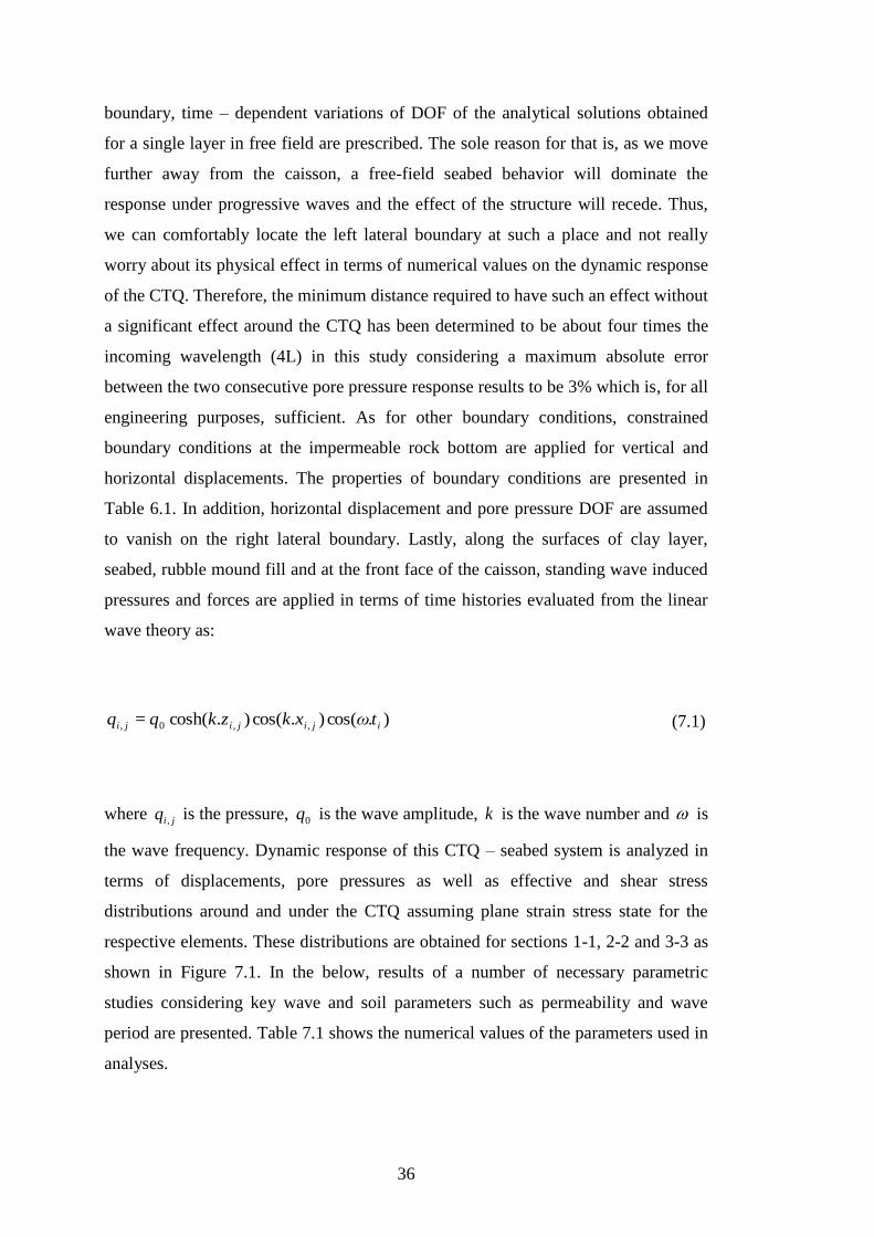
36
boundary, time – dependent variations of DOF of the analytical solutions obtained
for a single layer in free field are prescribed. The sole reason for that is, as we move
further away from the caisson, a free-field seabed behavior will dominate the
response under progressive waves and the effect of the structure will recede. Thus,
we can comfortably locate the left lateral boundary at such a place and not really
worry about its physical effect in terms of numerical values on the dynamic response
of the CTQ. Therefore, the minimum distance required to have such an effect without
a significant effect around the CTQ has been determined to be about four times the
incoming wavelength (4L) in this study considering a maximum absolute error
between the two consecutive pore pressure response results to be 3% which is, for all
engineering purposes, sufficient. As for other boundary conditions, constrained
boundary conditions at the impermeable rock bottom are applied for vertical and
horizontal displacements. The properties of boundary conditions are presented in
Table 6.1. In addition, horizontal displacement and pore pressure DOF are assumed
to vanish on the right lateral boundary. Lastly, along the surfaces of clay layer,
seabed, rubble mound fill and at the front face of the caisson, standing wave induced
pressures and forces are applied in terms of time histories evaluated from the linear
wave theory as:
).cos().cos().cosh(= ,,0, ijijiji tωxkzkqq (7.1)
where jiq , is the pressure, 0q is the wave amplitude, k is the wave number and is
the wave frequency. Dynamic response of this CTQ – seabed system is analyzed in
terms of displacements, pore pressures as well as effective and shear stress
distributions around and under the CTQ assuming plane strain stress state for the
respective elements. These distributions are obtained for sections 1-1, 2-2 and 3-3 as
shown in Figure 7.1. In the below, results of a number of necessary parametric
studies considering key wave and soil parameters such as permeability and wave
period are presented. Table 7.1 shows the numerical values of the parameters used in
analyses.

37
Table 7.1 : Numerical values of the parameters used in CTQ-Seabed analyses.
Properties Symbol Value (Unit)
Seabed Density γS 1.72 – 2.07 (t/m3)
Seabed Young‟s Modulus ES 16000-260000 (kPa)
Seabed Poisson‟s Ratio vS 0.3–0.33
Seabed Permeability kS 10-6
– 10-4
– 10-2
(m/s)
Seabed Porosity nS 0.28
Seabed Saturation SS 1
Clay Density γC 1.7 (t/m3)
Clay Young‟s Modulus EC 10330 (kPa)
Clay Poisson‟s Ratio vC 0.4
Clay Permeability kC 10-8
(m/s)
Clay Porosity nC 0.5
Clay Saturation SC 1
Rubble Density γR 2.00 (t/m3)
Rubble Young‟s Modulus ER 160000 (kPa)
Rubble Poisson‟s Ratio vR 0.33
Rubble Permeability kR 0.1 (m/s)
Rubble Porosity nR 0.25
Rubble Saturation SR 1
Caisson Density γW 2.5 (t/m3)
Caisson Young‟s Modulus EW 2x10⁷
(kPa)
Caisson Poisson‟s Ratio vW 0.18
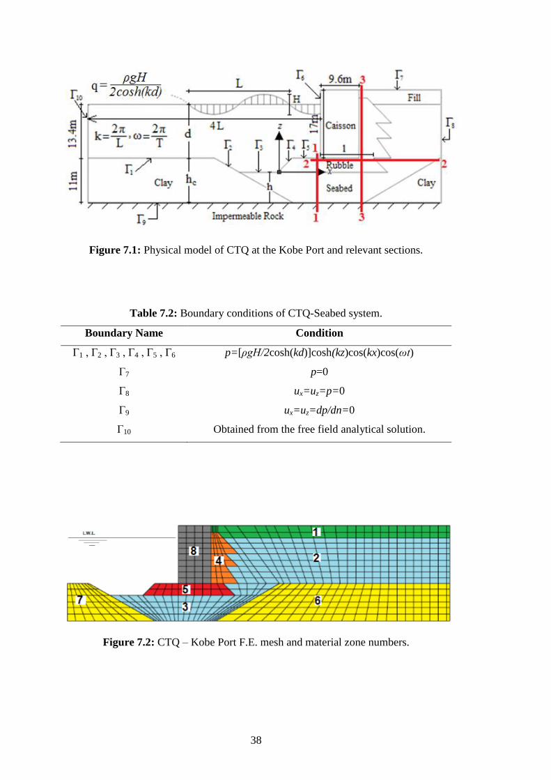
38
Figure 7.1: Physical model of CTQ at the Kobe Port and relevant sections.
Table 7.2: Boundary conditions of CTQ-Seabed system.
Boundary Name Condition
Г1 , Г2 , Г3 , Г4 , Г5 , Г6 p=[ρgH/2cosh(kd)]cosh(kz)cos(kx)cos(ωt)
Г7 p=0
Г8 ux=uz=p=0
Г9 ux=uz=dp/dn=0
Г10 Obtained from the free field analytical solution.
Figure 7.2: CTQ – Kobe Port F.E. mesh and material zone numbers.
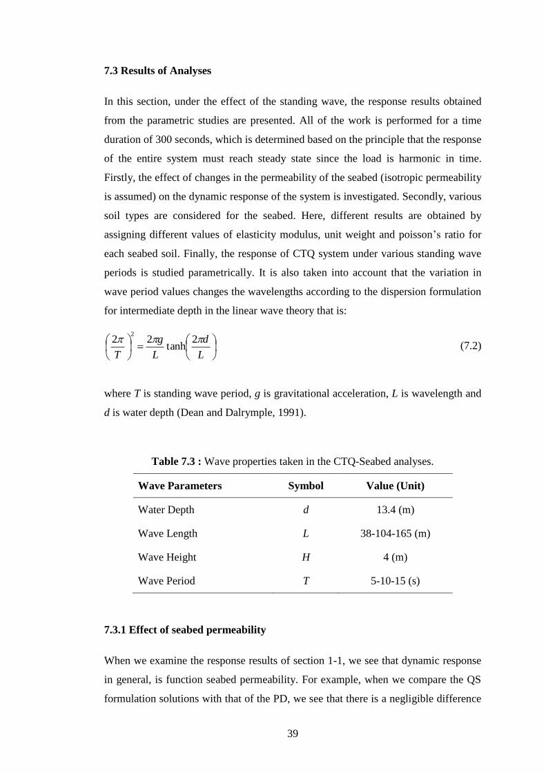
39
7.3 Results of Analyses
In this section, under the effect of the standing wave, the response results obtained
from the parametric studies are presented. All of the work is performed for a time
duration of 300 seconds, which is determined based on the principle that the response
of the entire system must reach steady state since the load is harmonic in time.
Firstly, the effect of changes in the permeability of the seabed (isotropic permeability
is assumed) on the dynamic response of the system is investigated. Secondly, various
soil types are considered for the seabed. Here, different results are obtained by
assigning different values of elasticity modulus, unit weight and poisson‟s ratio for
each seabed soil. Finally, the response of CTQ system under various standing wave
periods is studied parametrically. It is also taken into account that the variation in
wave period values changes the wavelengths according to the dispersion formulation
for intermediate depth in the linear wave theory that is:
L
d
L
g
T
2tanh
222
(7.2)
where T is standing wave period, g is gravitational acceleration, L is wavelength and
d is water depth (Dean and Dalrymple, 1991).
Table 7.3 : Wave properties taken in the CTQ-Seabed analyses.
Wave Parameters Symbol Value (Unit)
Water Depth d 13.4 (m)
Wave Length L 38-104-165 (m)
Wave Height H 4 (m)
Wave Period T 5-10-15 (s)
7.3.1 Effect of seabed permeability
When we examine the response results of section 1-1, we see that dynamic response
in general, is function seabed permeability. For example, when we compare the QS
formulation solutions with that of the PD, we see that there is a negligible difference
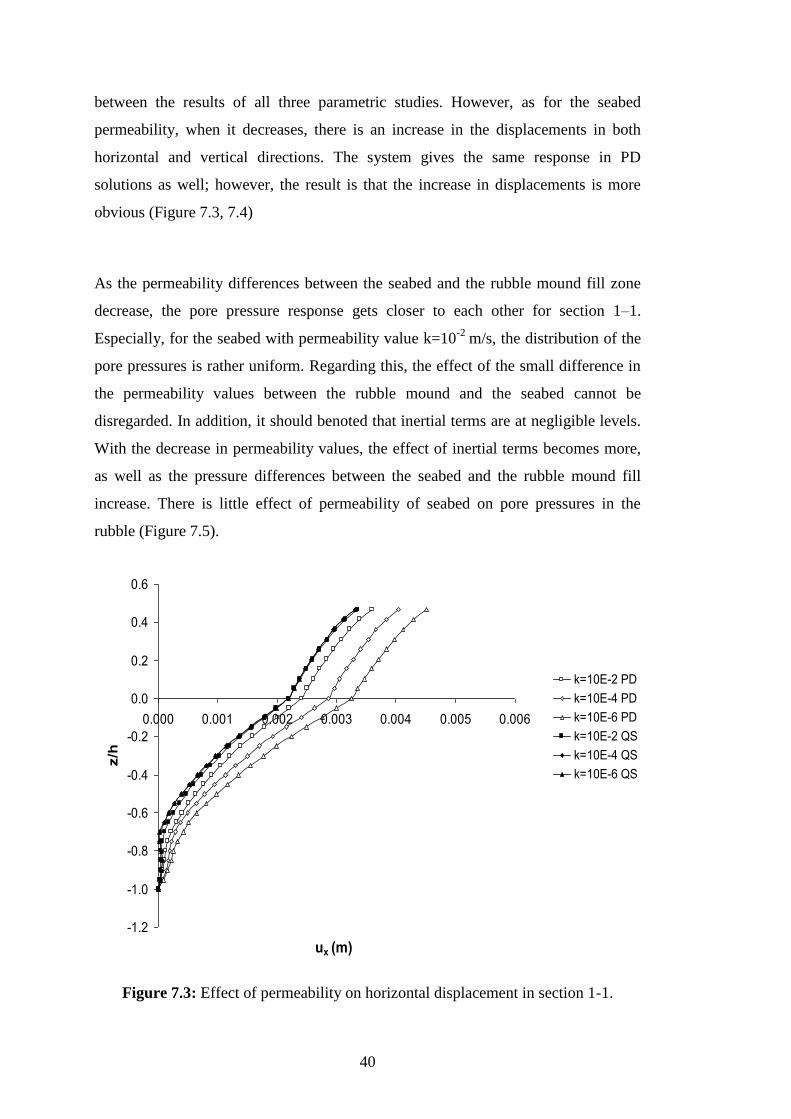
40
between the results of all three parametric studies. However, as for the seabed
permeability, when it decreases, there is an increase in the displacements in both
horizontal and vertical directions. The system gives the same response in PD
solutions as well; however, the result is that the increase in displacements is more
obvious (Figure 7.3, 7.4)
As the permeability differences between the seabed and the rubble mound fill zone
decrease, the pore pressure response gets closer to each other for section 1–1.
Especially, for the seabed with permeability value k=10-2
m/s, the distribution of the
pore pressures is rather uniform. Regarding this, the effect of the small difference in
the permeability values between the rubble mound and the seabed cannot be
disregarded. In addition, it should benoted that inertial terms are at negligible levels.
With the decrease in permeability values, the effect of inertial terms becomes more,
as well as the pressure differences between the seabed and the rubble mound fill
increase. There is little effect of permeability of seabed on pore pressures in the
rubble (Figure 7.5).
Figure 7.3: Effect of permeability on horizontal displacement in section 1-1.
-1.2
-1.0
-0.8
-0.6
-0.4
-0.2
0.0
0.2
0.4
0.6
0.000 0.001 0.002 0.003 0.004 0.005 0.006
ux (m)
z/h
k=10E-2 PD
k=10E-4 PD
k=10E-6 PD
k=10E-2 QS
k=10E-4 QS
k=10E-6 QS
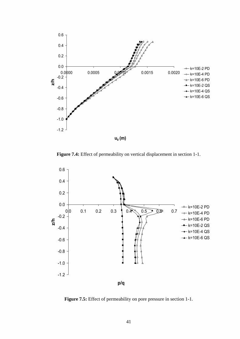
41
Figure 7.4: Effect of permeability on vertical displacement in section 1-1.
Figure 7.5: Effect of permeability on pore pressure in section 1-1.
-1.2
-1.0
-0.8
-0.6
-0.4
-0.2
0.0
0.2
0.4
0.6
0.0000 0.0005 0.0010 0.0015 0.0020
uz (m)
z/h
k=10E-2 PD
k=10E-4 PD
k=10E-6 PD
k=10E-2 QS
k=10E-4 QS
k=10E-6 QS
-1.2
-1.0
-0.8
-0.6
-0.4
-0.2
0.0
0.2
0.4
0.6
0.0 0.1 0.2 0.3 0.4 0.5 0.6 0.7
p/q
z/h
k=10E-2 PD
k=10E-4 PD
k=10E-6 PD
k=10E-2 QS
k=10E-4 QS
k=10E-6 QS
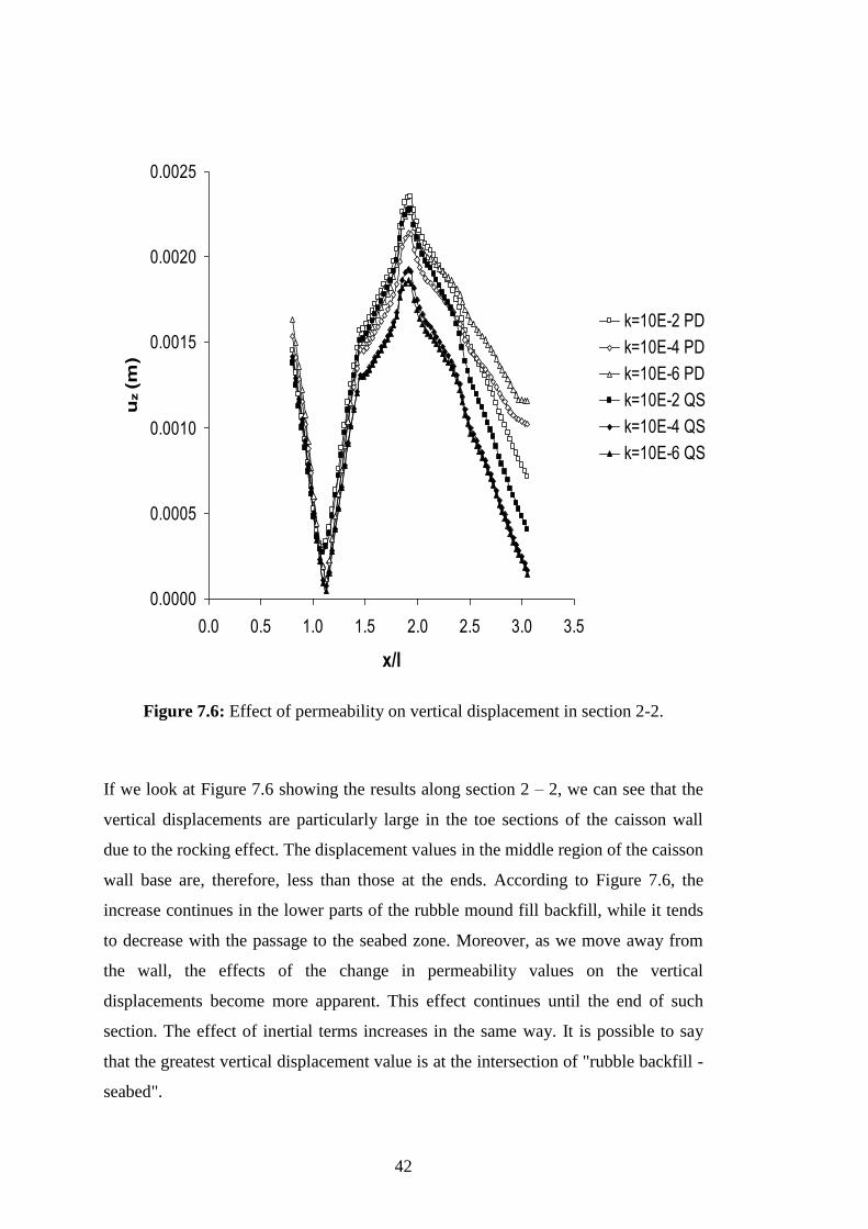
42
Figure 7.6: Effect of permeability on vertical displacement in section 2-2.
If we look at Figure 7.6 showing the results along section 2 – 2, we can see that the
vertical displacements are particularly large in the toe sections of the caisson wall
due to the rocking effect. The displacement values in the middle region of the caisson
wall base are, therefore, less than those at the ends. According to Figure 7.6, the
increase continues in the lower parts of the rubble mound fill backfill, while it tends
to decrease with the passage to the seabed zone. Moreover, as we move away from
the wall, the effects of the change in permeability values on the vertical
displacements become more apparent. This effect continues until the end of such
section. The effect of inertial terms increases in the same way. It is possible to say
that the greatest vertical displacement value is at the intersection of "rubble backfill -
seabed".
0.0000
0.0005
0.0010
0.0015
0.0020
0.0025
0.0 0.5 1.0 1.5 2.0 2.5 3.0 3.5
x/l
uz (m
)
k=10E-2 PD
k=10E-4 PD
k=10E-6 PD
k=10E-2 QS
k=10E-4 QS
k=10E-6 QS
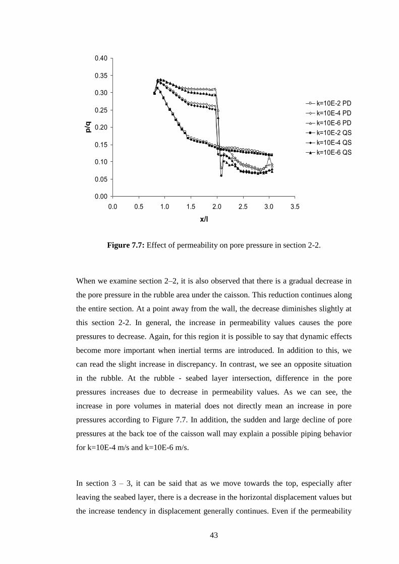
43
Figure 7.7: Effect of permeability on pore pressure in section 2-2.
When we examine section 2–2, it is also observed that there is a gradual decrease in
the pore pressure in the rubble area under the caisson. This reduction continues along
the entire section. At a point away from the wall, the decrease diminishes slightly at
this section 2-2. In general, the increase in permeability values causes the pore
pressures to decrease. Again, for this region it is possible to say that dynamic effects
become more important when inertial terms are introduced. In addition to this, we
can read the slight increase in discrepancy. In contrast, we see an opposite situation
in the rubble. At the rubble - seabed layer intersection, difference in the pore
pressures increases due to decrease in permeability values. As we can see, the
increase in pore volumes in material does not directly mean an increase in pore
pressures according to Figure 7.7. In addition, the sudden and large decline of pore
pressures at the back toe of the caisson wall may explain a possible piping behavior
for k=10E-4 m/s and k=10E-6 m/s.
In section 3 – 3, it can be said that as we move towards the top, especially after
leaving the seabed layer, there is a decrease in the horizontal displacement values but
the increase tendency in displacement generally continues. Even if the permeability
0.00
0.05
0.10
0.15
0.20
0.25
0.30
0.35
0.40
0.0 0.5 1.0 1.5 2.0 2.5 3.0 3.5
x/l
p/q
k=10E-2 PD
k=10E-4 PD
k=10E-6 PD
k=10E-2 QS
k=10E-4 QS
k=10E-6 QS
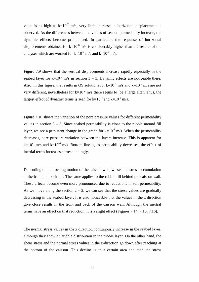
44
value is as high as k=10-2
m/s, very little increase in horizontal displacement is
observed. As the differences between the values of seabed permeability increase, the
dynamic effects become pronounced. In particular, the response of horizontal
displacements obtained for k=10-6
m/s is considerably higher than the results of the
analyses which are worked for k=10-4
m/s and k=10-2
m/s.
Figure 7.9 shows that the vertical displacements increase rapidly especially in the
seabed layer for k=10-2
m/s in section 3 – 3. Dynamic effects are noticeable there.
Also, in this figure, the results in QS solutions for k=10-4
m/s and k=10-6
m/s are not
very different, nevertheless for k=10-2
m/s there seems to be a large alter. Thus, the
largest effect of dynamic terms is seen for k=10-4
and k=10-6
m/s.
Figure 7.10 shows the variation of the pore pressure values for different permeability
values in section 3 – 3. Since seabed permeability is close to the rubble mound fill
layer, we see a persistent change in the graph for k=10-2
m/s. When the permeability
decreases, pore pressure variation between the layers increase. This is apparent for
k=10-4
m/s and k=10-6
m/s. Bottom line is, as permeability decreases, the effect of
inertial terms increases correspondingly.
Depending on the rocking motion of the caisson wall, we see the stress accumulation
at the front and back toe. The same applies to the rubble fill behind the caisson wall.
These effects become even more pronounced due to reductions in soil permeability.
As we move along the section 2 – 2, we can see that the stress values are gradually
decreasing in the seabed layer. It is also noticeable that the values in the z direction
give close results in the front and back of the caisson wall. Although the inertial
terms have an effect on that reduction, it is a slight effect (Figures 7.14, 7.15, 7.16).
The normal stress values in the x direction continuously increase in the seabed layer,
although they show a variable distribution in the rubble layer. On the other hand, the
shear stress and the normal stress values in the z-direction go down after reaching at
the bottom of the caisson. This decline is in a certain area and then the stress

45
responses ascend again towards the fill. Then, it suddenly gets reduced again.
Furthermore, in the rubble layer, there is no effect on the shear stresses of the soil
permeability (Figures 7.17, 7.18, 7.19).
Figure 7.8: Effect of permeability on horizontal displacement in section 3-3.
Figure 7.9: Effect of permeability on vertical displacement in section 3-3.
-1.5
-1.0
-0.5
0.0
0.5
1.0
1.5
2.0
2.5
3.0
-0.001 0.000 0.001 0.002 0.003 0.004 0.005 0.006
ux (m)
z/h
k=10E-2 PD
k=10E-4 PD
k=10E-6 PD
k=10E-2 QS
k=10E-4 QS
k=10E-6 QS
-1.5
-1.0
-0.5
0.0
0.5
1.0
1.5
2.0
2.5
3.0
0.0000 0.0004 0.0008 0.0012 0.0016 0.0020
uz (m)
z/h
k=10E-2 PD
k=10E-4 PD
k=10E-6 PD
k=10E-2 QS
k=10E-4 QS
k=10E-6 QS
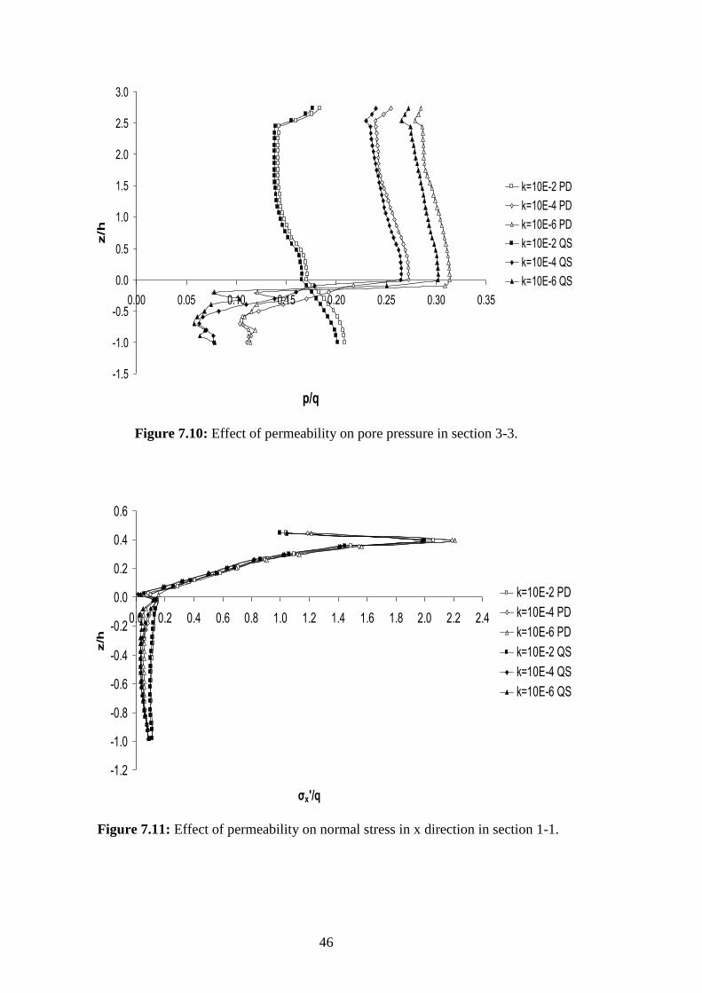
46
Figure 7.10: Effect of permeability on pore pressure in section 3-3.
Figure 7.11: Effect of permeability on normal stress in x direction in section 1-1.
-1.5
-1.0
-0.5
0.0
0.5
1.0
1.5
2.0
2.5
3.0
0.00 0.05 0.10 0.15 0.20 0.25 0.30 0.35
p/q
z/h
k=10E-2 PD
k=10E-4 PD
k=10E-6 PD
k=10E-2 QS
k=10E-4 QS
k=10E-6 QS
-1.2
-1.0
-0.8
-0.6
-0.4
-0.2
0.0
0.2
0.4
0.6
0.0 0.2 0.4 0.6 0.8 1.0 1.2 1.4 1.6 1.8 2.0 2.2 2.4
σx'/q
z/h
k=10E-2 PD
k=10E-4 PD
k=10E-6 PD
k=10E-2 QS
k=10E-4 QS
k=10E-6 QS
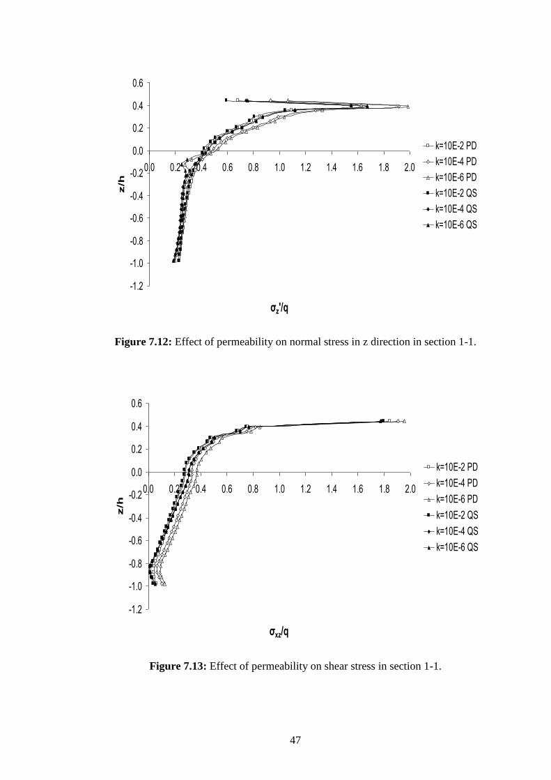
47
Figure 7.12: Effect of permeability on normal stress in z direction in section 1-1.
Figure 7.13: Effect of permeability on shear stress in section 1-1.
-1.2
-1.0
-0.8
-0.6
-0.4
-0.2
0.0
0.2
0.4
0.6
0.0 0.2 0.4 0.6 0.8 1.0 1.2 1.4 1.6 1.8 2.0
σz'/q
z/h
k=10E-2 PD
k=10E-4 PD
k=10E-6 PD
k=10E-2 QS
k=10E-4 QS
k=10E-6 QS
-1.2
-1.0
-0.8
-0.6
-0.4
-0.2
0.0
0.2
0.4
0.6
0.0 0.2 0.4 0.6 0.8 1.0 1.2 1.4 1.6 1.8 2.0
σxz/q
z/h
k=10E-2 PD
k=10E-4 PD
k=10E-6 PD
k=10E-2 QS
k=10E-4 QS
k=10E-6 QS
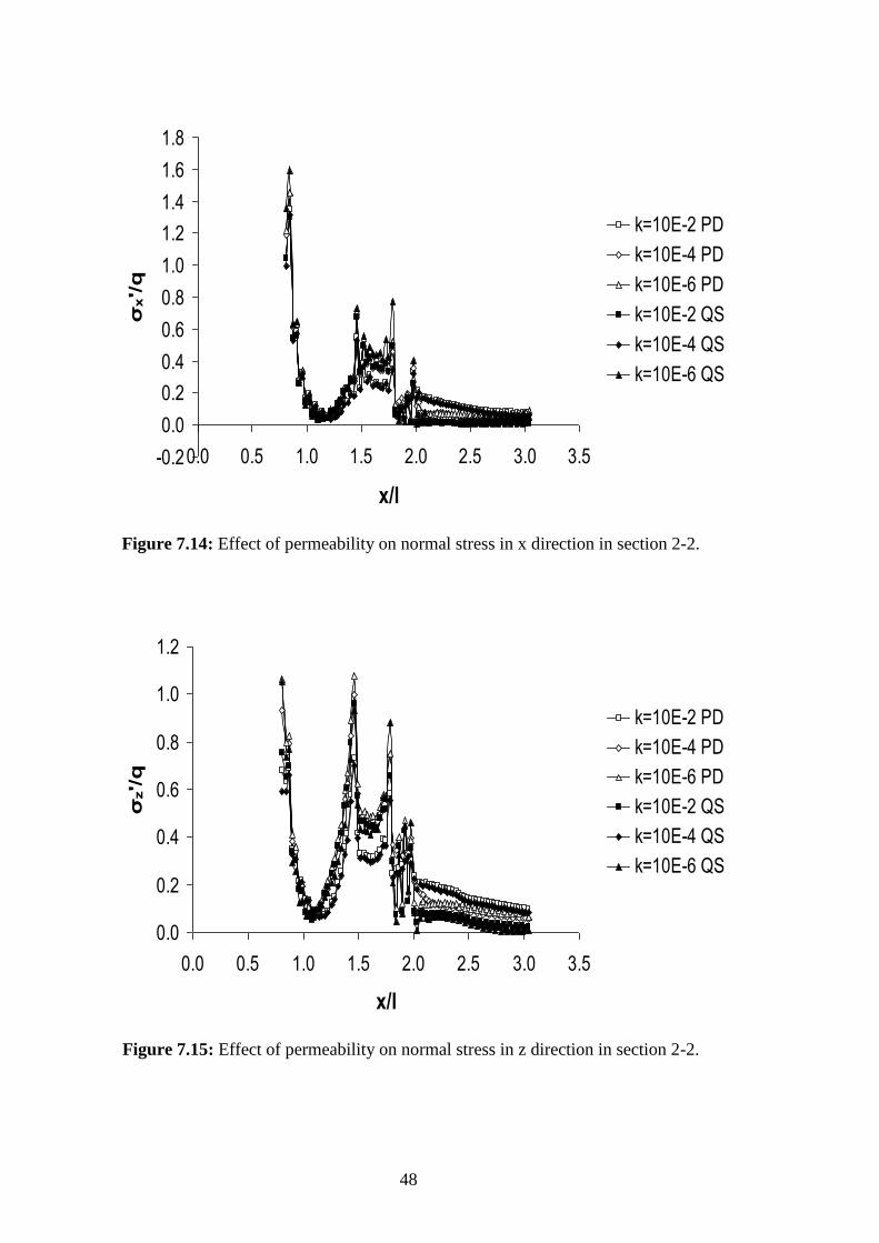
48
Figure 7.14: Effect of permeability on normal stress in x direction in section 2-2.
Figure 7.15: Effect of permeability on normal stress in z direction in section 2-2.
-0.2
0.0
0.2
0.4
0.6
0.8
1.0
1.2
1.4
1.6
1.8
0.0 0.5 1.0 1.5 2.0 2.5 3.0 3.5
x/l
σx'/q
k=10E-2 PD
k=10E-4 PD
k=10E-6 PD
k=10E-2 QS
k=10E-4 QS
k=10E-6 QS
0.0
0.2
0.4
0.6
0.8
1.0
1.2
0.0 0.5 1.0 1.5 2.0 2.5 3.0 3.5
x/l
σz'/q
k=10E-2 PD
k=10E-4 PD
k=10E-6 PD
k=10E-2 QS
k=10E-4 QS
k=10E-6 QS
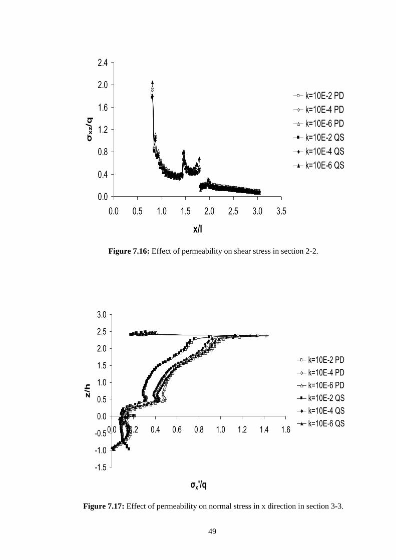
49
Figure 7.16: Effect of permeability on shear stress in section 2-2.
Figure 7.17: Effect of permeability on normal stress in x direction in section 3-3.
0.0
0.4
0.8
1.2
1.6
2.0
2.4
0.0 0.5 1.0 1.5 2.0 2.5 3.0 3.5
x/l
σx
z/q
k=10E-2 PD
k=10E-4 PD
k=10E-6 PD
k=10E-2 QS
k=10E-4 QS
k=10E-6 QS
-1.5
-1.0
-0.5
0.0
0.5
1.0
1.5
2.0
2.5
3.0
0.0 0.2 0.4 0.6 0.8 1.0 1.2 1.4 1.6
σx'/q
z/h
k=10E-2 PD
k=10E-4 PD
k=10E-6 PD
k=10E-2 QS
k=10E-4 QS
k=10E-6 QS
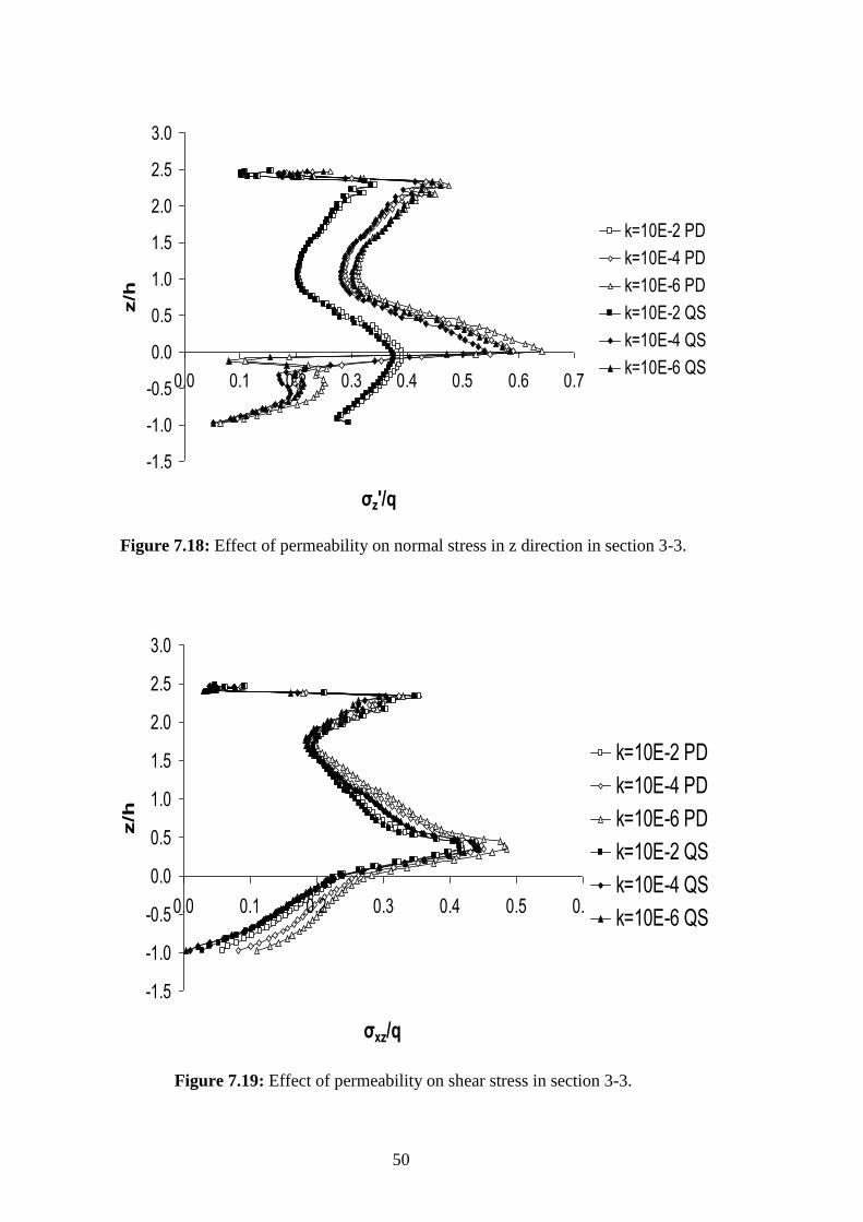
50
Figure 7.18: Effect of permeability on normal stress in z direction in section 3-3.
Figure 7.19: Effect of permeability on shear stress in section 3-3.
-1.5
-1.0
-0.5
0.0
0.5
1.0
1.5
2.0
2.5
3.0
0.0 0.1 0.2 0.3 0.4 0.5 0.6 0.7
σz'/q
z/h
k=10E-2 PD
k=10E-4 PD
k=10E-6 PD
k=10E-2 QS
k=10E-4 QS
k=10E-6 QS
-1.5
-1.0
-0.5
0.0
0.5
1.0
1.5
2.0
2.5
3.0
0.0 0.1 0.2 0.3 0.4 0.5 0.6
σxz/q
z/h
k=10E-2 PD
k=10E-4 PD
k=10E-6 PD
k=10E-2 QS
k=10E-4 QS
k=10E-6 QS
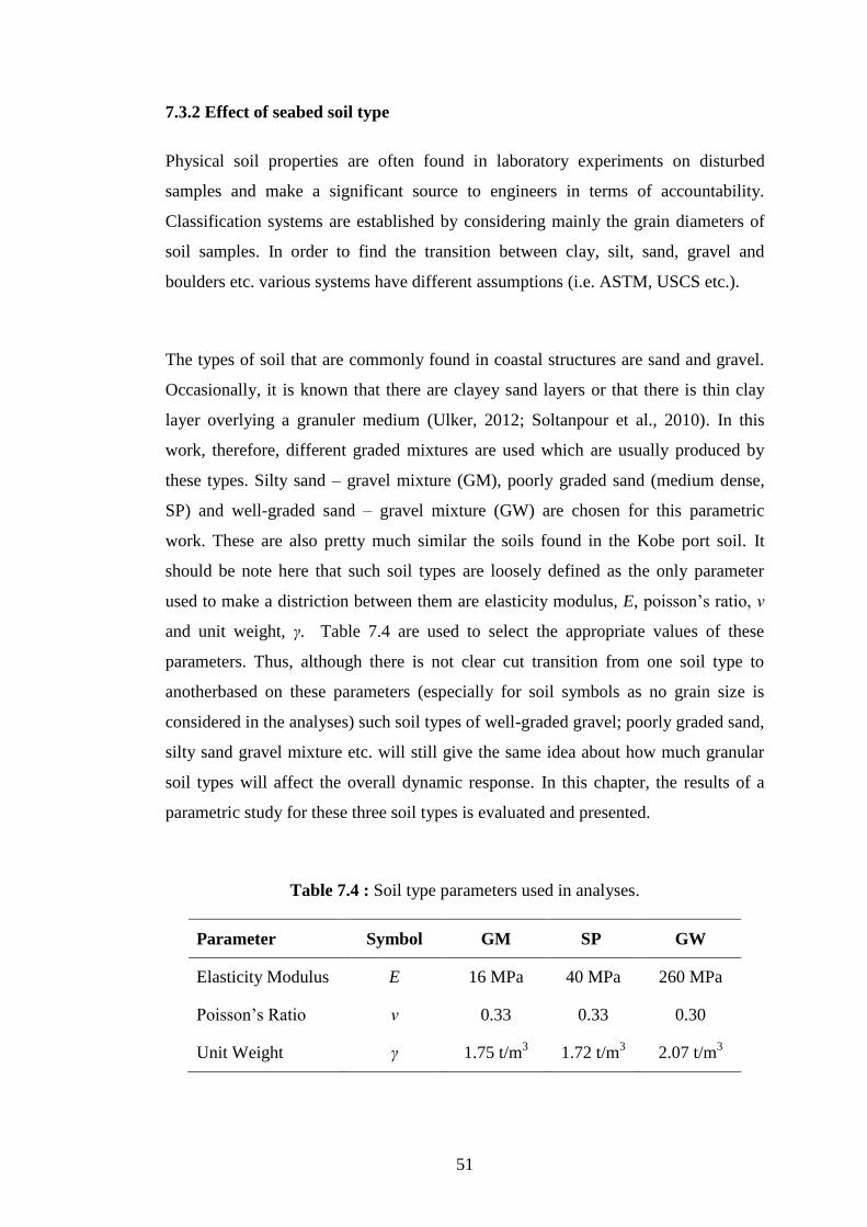
51
7.3.2 Effect of seabed soil type
Physical soil properties are often found in laboratory experiments on disturbed
samples and make a significant source to engineers in terms of accountability.
Classification systems are established by considering mainly the grain diameters of
soil samples. In order to find the transition between clay, silt, sand, gravel and
boulders etc. various systems have different assumptions (i.e. ASTM, USCS etc.).
The types of soil that are commonly found in coastal structures are sand and gravel.
Occasionally, it is known that there are clayey sand layers or that there is thin clay
layer overlying a granuler medium (Ulker, 2012; Soltanpour et al., 2010). In this
work, therefore, different graded mixtures are used which are usually produced by
these types. Silty sand – gravel mixture (GM), poorly graded sand (medium dense,
SP) and well-graded sand – gravel mixture (GW) are chosen for this parametric
work. These are also pretty much similar the soils found in the Kobe port soil. It
should be note here that such soil types are loosely defined as the only parameter
used to make a distriction between them are elasticity modulus, E, poisson‟s ratio, ν
and unit weight, γ. Table 7.4 are used to select the appropriate values of these
parameters. Thus, although there is not clear cut transition from one soil type to
anotherbased on these parameters (especially for soil symbols as no grain size is
considered in the analyses) such soil types of well-graded gravel; poorly graded sand,
silty sand gravel mixture etc. will still give the same idea about how much granular
soil types will affect the overall dynamic response. In this chapter, the results of a
parametric study for these three soil types is evaluated and presented.
Table 7.4 : Soil type parameters used in analyses.
Parameter Symbol GM SP GW
Elasticity Modulus E 16 MPa 40 MPa 260 MPa
Poisson‟s Ratio ν 0.33 0.33 0.30
Unit Weight γ 1.75 t/m3 1.72 t/m
3 2.07 t/m
3

52
When the displacements are examined, the effect of inertial terms in the PD solution
becomes more pronounced with the change of soil types. In section 1 – 1, between
PD and QS solutions, low differences occur in the response for well-graded dense
sand – gravel mixture (GW). It can be said that the reason for this is that the GW
contains less space than other types of soil, although the permeability values are the
same. According to the results from analyses made specifically for poorly graded
sand (SP) and silty sand – gravel mixture (GM), inertial terms play an effective role
on both horizontal and vertical displacements. In addition, the increase in
discrepancy, especially in vertical displacements, can be emphasized and is more
pronounced in the variation of horizontal displacement. Another result that can be
deduced from these figures is the observable decrease in displacement when moving
to the rubble zone (Figure 7.20 and 7.21).
Figure 7.22 shows the changes in pore pressure normalized by the standing wave
amplitude in the rubble mound fill and seabed layers compared to the different soil
types in section 1 – 1. In view of that, changes in soil types do not lead to a
significant difference in the rubble mound layer. In this context, it can be said that
what is important for the rubble mound layer is its granulometry. So, no matter how
much the soil type in the lower layer varies, the upper rubble layer is not affected by
this, considering the pore pressure differences. In addition, the dynamic terms have
little effect in that section also. Alternatively, the effect of these terms is apparent in
the seabed layer.
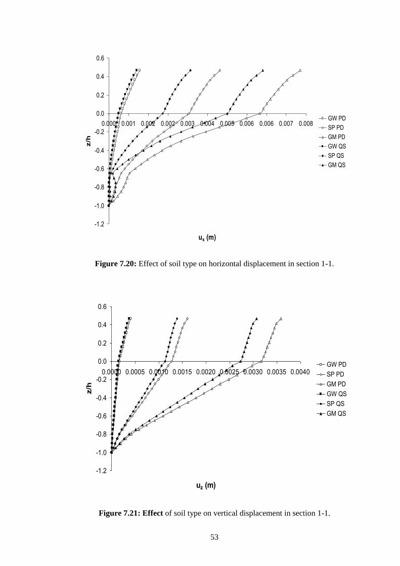
53
Figure 7.20: Effect of soil type on horizontal displacement in section 1-1.
Figure 7.21: Effect of soil type on vertical displacement in section 1-1.
-1.2
-1.0
-0.8
-0.6
-0.4
-0.2
0.0
0.2
0.4
0.6
0.000 0.001 0.002 0.002 0.003 0.004 0.005 0.006 0.006 0.007 0.008
ux (m)
z/h
GW PD
SP PD
GM PD
GW QS
SP QS
GM QS
-1.2
-1.0
-0.8
-0.6
-0.4
-0.2
0.0
0.2
0.4
0.6
0.0000 0.0005 0.0010 0.0015 0.0020 0.0025 0.0030 0.0035 0.0040
uz (m)
z/h
GW PD
SP PD
GM PD
GW QS
SP QS
GM QS
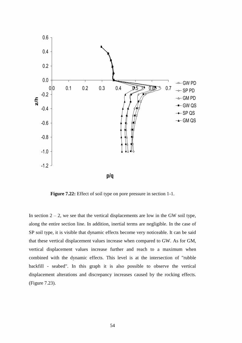
54
Figure 7.22: Effect of soil type on pore pressure in section 1-1.
In section 2 – 2, we see that the vertical displacements are low in the GW soil type,
along the entire section line. In addition, inertial terms are negligible. In the case of
SP soil type, it is visible that dynamic effects become very noticeable. It can be said
that these vertical displacement values increase when compared to GW. As for GM,
vertical displacement values increase further and reach to a maximum when
combined with the dynamic effects. This level is at the intersection of "rubble
backfill - seabed". In this graph it is also possible to observe the vertical
displacement alterations and discrepancy increases caused by the rocking effects.
(Figure 7.23).
-1.2
-1.0
-0.8
-0.6
-0.4
-0.2
0.0
0.2
0.4
0.6
0.0 0.1 0.2 0.3 0.4 0.5 0.6 0.7
p/q
z/h
GW PD
SP PD
GM PD
GW QS
SP QS
GM QS
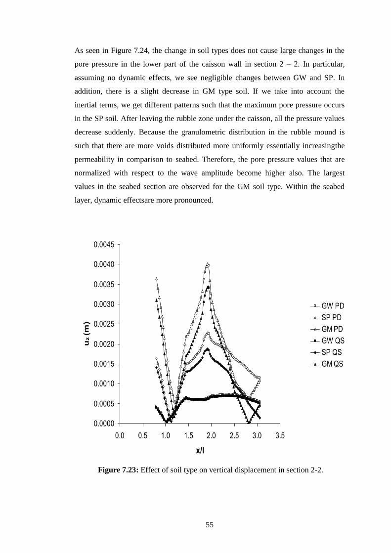
55
As seen in Figure 7.24, the change in soil types does not cause large changes in the
pore pressure in the lower part of the caisson wall in section 2 – 2. In particular,
assuming no dynamic effects, we see negligible changes between GW and SP. In
addition, there is a slight decrease in GM type soil. If we take into account the
inertial terms, we get different patterns such that the maximum pore pressure occurs
in the SP soil. After leaving the rubble zone under the caisson, all the pressure values
decrease suddenly. Because the granulometric distribution in the rubble mound is
such that there are more voids distributed more uniformly essentially increasingthe
permeability in comparison to seabed. Therefore, the pore pressure values that are
normalized with respect to the wave amplitude become higher also. The largest
values in the seabed section are observed for the GM soil type. Within the seabed
layer, dynamic effectsare more pronounced.
Figure 7.23: Effect of soil type on vertical displacement in section 2-2.
0.0000
0.0005
0.0010
0.0015
0.0020
0.0025
0.0030
0.0035
0.0040
0.0045
0.0 0.5 1.0 1.5 2.0 2.5 3.0 3.5
x/l
uz (m
)
GW PD
SP PD
GM PD
GW QS
SP QS
GM QS
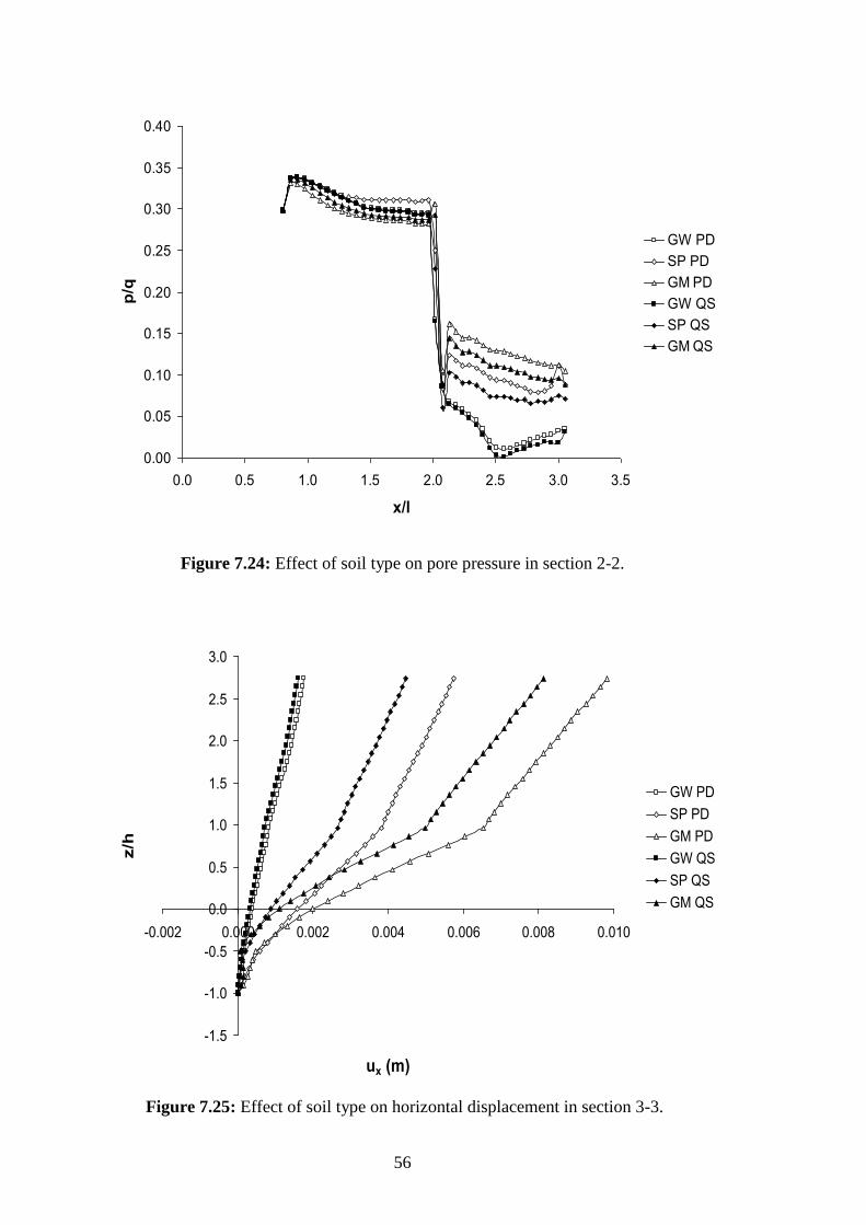
56
Figure 7.24: Effect of soil type on pore pressure in section 2-2.
Figure 7.25: Effect of soil type on horizontal displacement in section 3-3.
0.00
0.05
0.10
0.15
0.20
0.25
0.30
0.35
0.40
0.0 0.5 1.0 1.5 2.0 2.5 3.0 3.5
x/l
p/q
GW PD
SP PD
GM PD
GW QS
SP QS
GM QS
-1.5
-1.0
-0.5
0.0
0.5
1.0
1.5
2.0
2.5
3.0
-0.002 0.000 0.002 0.004 0.006 0.008 0.010
ux (m)
z/h
GW PD
SP PD
GM PD
GW QS
SP QS
GM QS
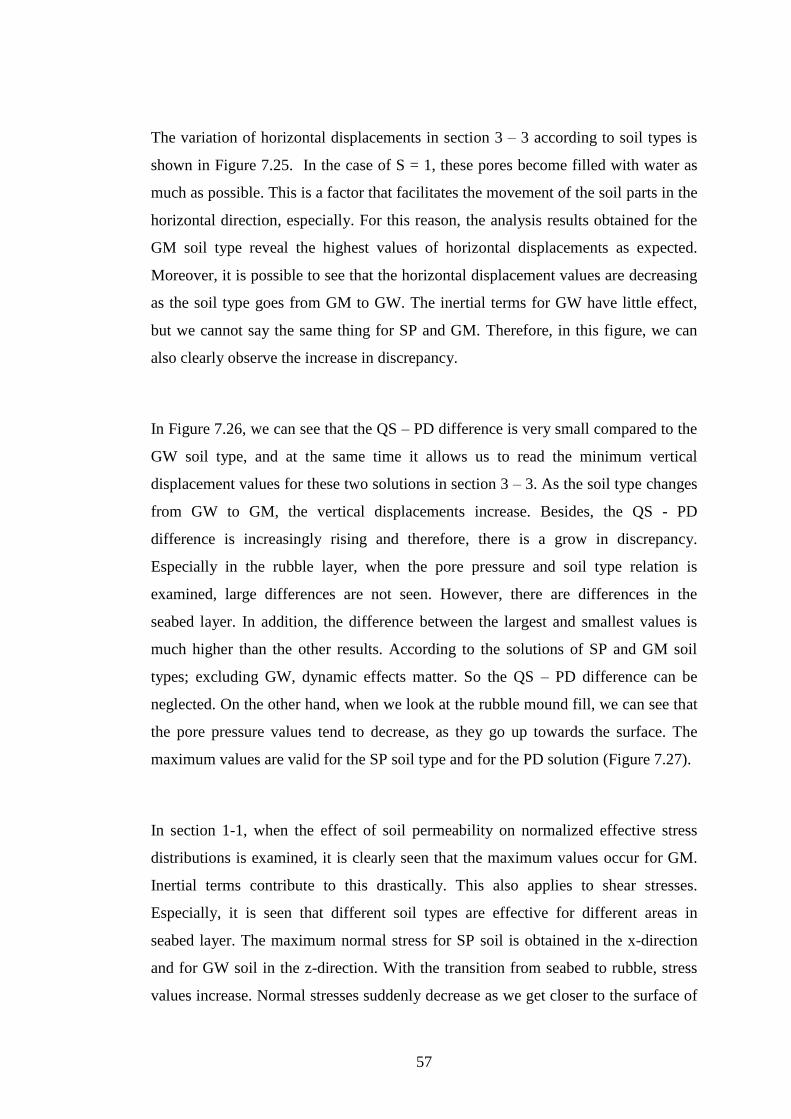
57
The variation of horizontal displacements in section 3 – 3 according to soil types is
shown in Figure 7.25. In the case of S = 1, these pores become filled with water as
much as possible. This is a factor that facilitates the movement of the soil parts in the
horizontal direction, especially. For this reason, the analysis results obtained for the
GM soil type reveal the highest values of horizontal displacements as expected.
Moreover, it is possible to see that the horizontal displacement values are decreasing
as the soil type goes from GM to GW. The inertial terms for GW have little effect,
but we cannot say the same thing for SP and GM. Therefore, in this figure, we can
also clearly observe the increase in discrepancy.
In Figure 7.26, we can see that the QS – PD difference is very small compared to the
GW soil type, and at the same time it allows us to read the minimum vertical
displacement values for these two solutions in section 3 – 3. As the soil type changes
from GW to GM, the vertical displacements increase. Besides, the QS - PD
difference is increasingly rising and therefore, there is a grow in discrepancy.
Especially in the rubble layer, when the pore pressure and soil type relation is
examined, large differences are not seen. However, there are differences in the
seabed layer. In addition, the difference between the largest and smallest values is
much higher than the other results. According to the solutions of SP and GM soil
types; excluding GW, dynamic effects matter. So the QS – PD difference can be
neglected. On the other hand, when we look at the rubble mound fill, we can see that
the pore pressure values tend to decrease, as they go up towards the surface. The
maximum values are valid for the SP soil type and for the PD solution (Figure 7.27).
In section 1-1, when the effect of soil permeability on normalized effective stress
distributions is examined, it is clearly seen that the maximum values occur for GM.
Inertial terms contribute to this drastically. This also applies to shear stresses.
Especially, it is seen that different soil types are effective for different areas in
seabed layer. The maximum normal stress for SP soil is obtained in the x-direction
and for GW soil in the z-direction. With the transition from seabed to rubble, stress
values increase. Normal stresses suddenly decrease as we get closer to the surface of
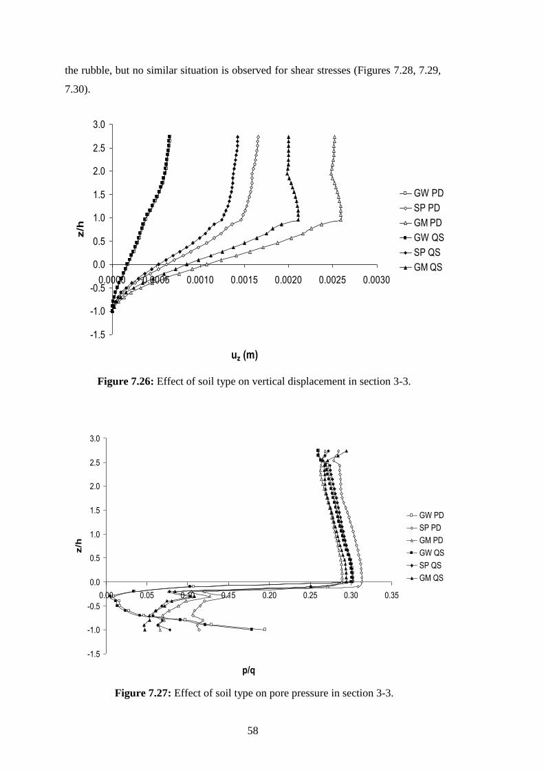
58
the rubble, but no similar situation is observed for shear stresses (Figures 7.28, 7.29,
7.30).
Figure 7.26: Effect of soil type on vertical displacement in section 3-3.
Figure 7.27: Effect of soil type on pore pressure in section 3-3.
-1.5
-1.0
-0.5
0.0
0.5
1.0
1.5
2.0
2.5
3.0
0.0000 0.0005 0.0010 0.0015 0.0020 0.0025 0.0030
uz (m)
z/h
GW PD
SP PD
GM PD
GW QS
SP QS
GM QS
-1.5
-1.0
-0.5
0.0
0.5
1.0
1.5
2.0
2.5
3.0
0.00 0.05 0.10 0.15 0.20 0.25 0.30 0.35
p/q
z/h
GW PD
SP PD
GM PD
GW QS
SP QS
GM QS
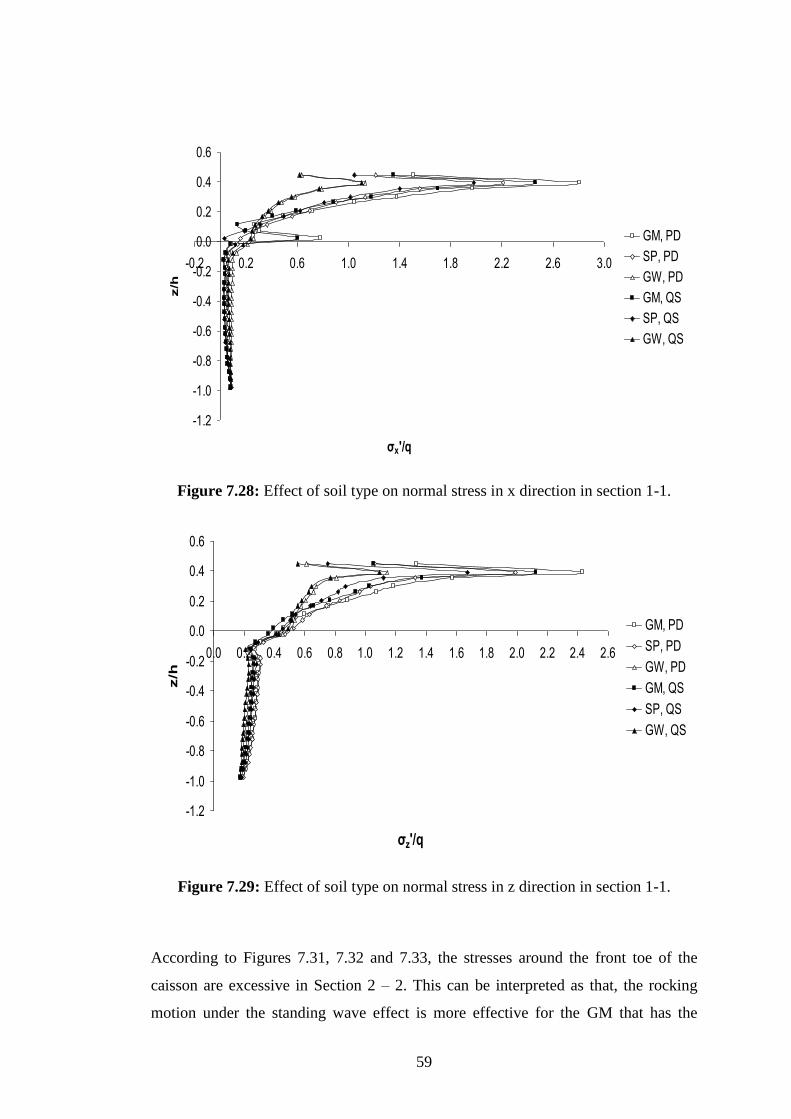
59
Figure 7.28: Effect of soil type on normal stress in x direction in section 1-1.
Figure 7.29: Effect of soil type on normal stress in z direction in section 1-1.
According to Figures 7.31, 7.32 and 7.33, the stresses around the front toe of the
caisson are excessive in Section 2 – 2. This can be interpreted as that, the rocking
motion under the standing wave effect is more effective for the GM that has the
-1.2
-1.0
-0.8
-0.6
-0.4
-0.2
0.0
0.2
0.4
0.6
-0.2 0.2 0.6 1.0 1.4 1.8 2.2 2.6 3.0
σx'/q
z/h
GM, PD
SP, PD
GW, PD
GM, QS
SP, QS
GW, QS
-1.2
-1.0
-0.8
-0.6
-0.4
-0.2
0.0
0.2
0.4
0.6
0.0 0.2 0.4 0.6 0.8 1.0 1.2 1.4 1.6 1.8 2.0 2.2 2.4 2.6
σz'/q
z/h
GM, PD
SP, PD
GW, PD
GM, QS
SP, QS
GW, QS
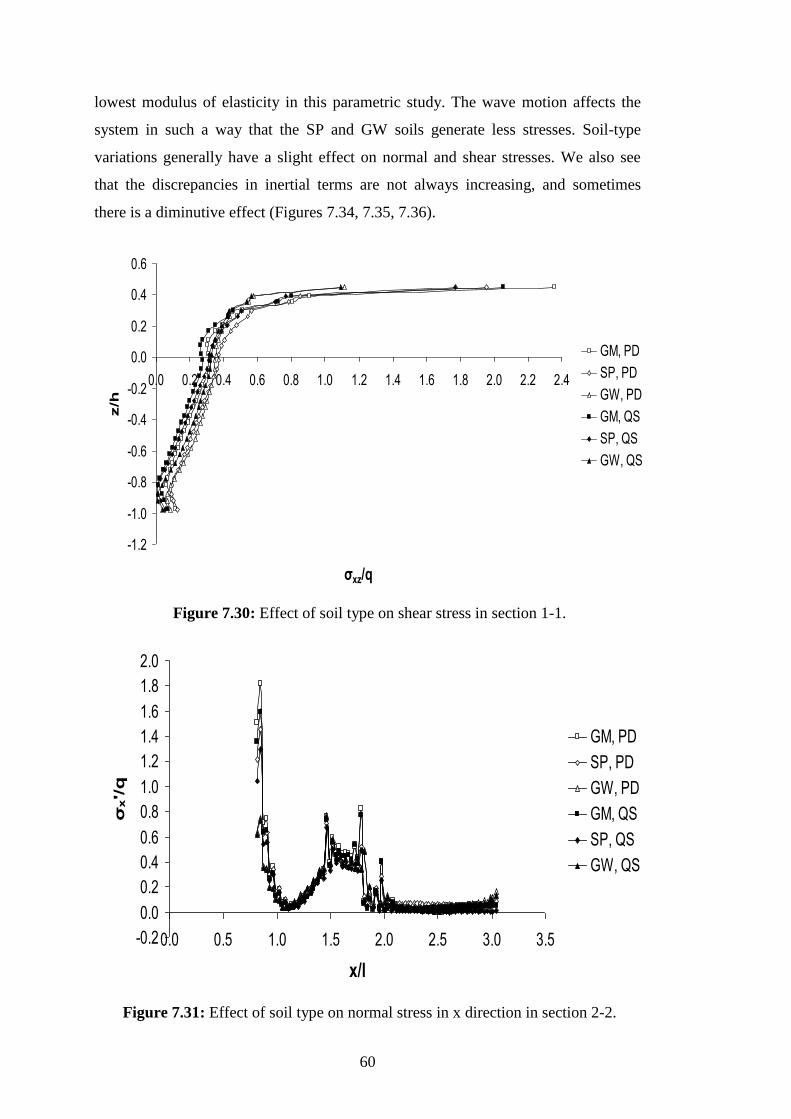
60
lowest modulus of elasticity in this parametric study. The wave motion affects the
system in such a way that the SP and GW soils generate less stresses. Soil-type
variations generally have a slight effect on normal and shear stresses. We also see
that the discrepancies in inertial terms are not always increasing, and sometimes
there is a diminutive effect (Figures 7.34, 7.35, 7.36).
Figure 7.30: Effect of soil type on shear stress in section 1-1.
Figure 7.31: Effect of soil type on normal stress in x direction in section 2-2.
-1.2
-1.0
-0.8
-0.6
-0.4
-0.2
0.0
0.2
0.4
0.6
0.0 0.2 0.4 0.6 0.8 1.0 1.2 1.4 1.6 1.8 2.0 2.2 2.4
σxz/q
z/h
GM, PD
SP, PD
GW, PD
GM, QS
SP, QS
GW, QS
-0.2
0.0
0.2
0.4
0.6
0.8
1.0
1.2
1.4
1.6
1.8
2.0
0.0 0.5 1.0 1.5 2.0 2.5 3.0 3.5
x/l
σx'/q
GM, PD
SP, PD
GW, PD
GM, QS
SP, QS
GW, QS
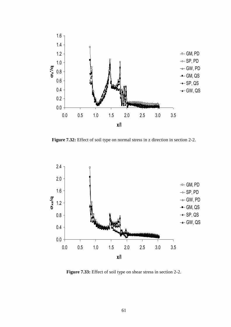
61
Figure 7.32: Effect of soil type on normal stress in z direction in section 2-2.
Figure 7.33: Effect of soil type on shear stress in section 2-2.
0.0
0.2
0.4
0.6
0.8
1.0
1.2
1.4
1.6
0.0 0.5 1.0 1.5 2.0 2.5 3.0 3.5
x/l
σz'/q
GM, PD
SP, PD
GW, PD
GM, QS
SP, QS
GW, QS
0.0
0.4
0.8
1.2
1.6
2.0
2.4
0.0 0.5 1.0 1.5 2.0 2.5 3.0 3.5
x/l
σx
z/q
GM, PD
SP, PD
GW, PD
GM, QS
SP, QS
GW, QS
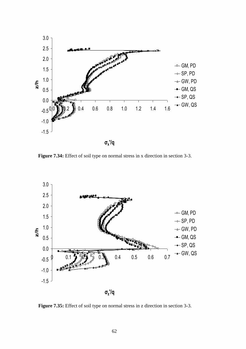
62
Figure 7.34: Effect of soil type on normal stress in x direction in section 3-3.
Figure 7.35: Effect of soil type on normal stress in z direction in section 3-3.
-1.5
-1.0
-0.5
0.0
0.5
1.0
1.5
2.0
2.5
3.0
0.0 0.2 0.4 0.6 0.8 1.0 1.2 1.4 1.6
σx'/q
z/h
GM, PD
SP, PD
GW, PD
GM, QS
SP, QS
GW, QS
-1.5
-1.0
-0.5
0.0
0.5
1.0
1.5
2.0
2.5
3.0
0 0.1 0.2 0.3 0.4 0.5 0.6 0.7
σz'/q
z/h
GM, PD
SP, PD
GW, PD
GM, QS
SP, QS
GW, QS
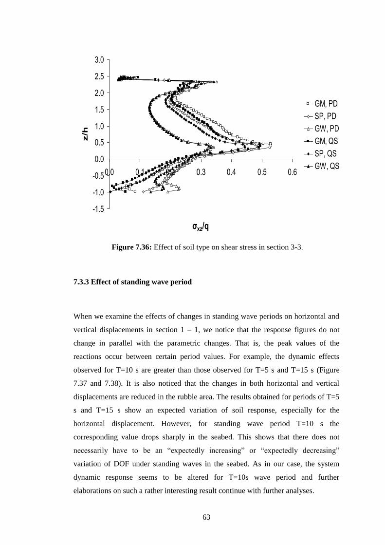
63
Figure 7.36: Effect of soil type on shear stress in section 3-3.
7.3.3 Effect of standing wave period
When we examine the effects of changes in standing wave periods on horizontal and
vertical displacements in section 1 – 1, we notice that the response figures do not
change in parallel with the parametric changes. That is, the peak values of the
reactions occur between certain period values. For example, the dynamic effects
observed for T=10 s are greater than those observed for T=5 s and T=15 s (Figure
7.37 and 7.38). It is also noticed that the changes in both horizontal and vertical
displacements are reduced in the rubble area. The results obtained for periods of T=5
s and T=15 s show an expected variation of soil response, especially for the
horizontal displacement. However, for standing wave period T=10 s the
corresponding value drops sharply in the seabed. This shows that there does not
necessarily have to be an “expectedly increasing” or “expectedly decreasing”
variation of DOF under standing waves in the seabed. As in our case, the system
dynamic response seems to be altered for T=10s wave period and further
elaborations on such a rather interesting result continue with further analyses.
-1.5
-1.0
-0.5
0.0
0.5
1.0
1.5
2.0
2.5
3.0
0.0 0.1 0.2 0.3 0.4 0.5 0.6
σxz/q
z/h
GM, PD
SP, PD
GW, PD
GM, QS
SP, QS
GW, QS
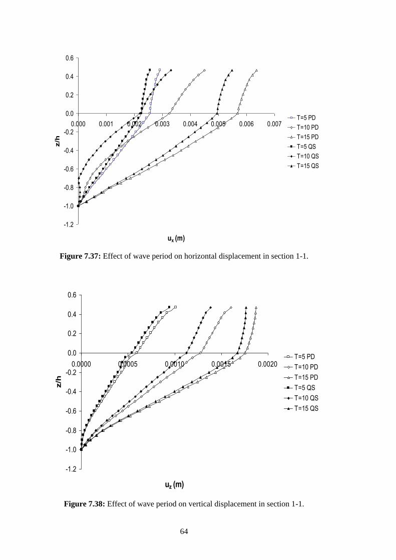
64
Figure 7.37: Effect of wave period on horizontal displacement in section 1-1.
Figure 7.38: Effect of wave period on vertical displacement in section 1-1.
-1.2
-1.0
-0.8
-0.6
-0.4
-0.2
0.0
0.2
0.4
0.6
0.000 0.001 0.002 0.003 0.004 0.005 0.006 0.007
ux (m)
z/h
T=5 PD
T=10 PD
T=15 PD
T=5 QS
T=10 QS
T=15 QS
-1.2
-1.0
-0.8
-0.6
-0.4
-0.2
0.0
0.2
0.4
0.6
0.0000 0.0005 0.0010 0.0015 0.0020
uz (m)
z/h
T=5 PD
T=10 PD
T=15 PD
T=5 QS
T=10 QS
T=15 QS
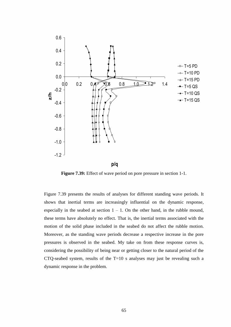
65
Figure 7.39: Effect of wave period on pore pressure in section 1-1.
Figure 7.39 presents the results of analyses for different standing wave periods. It
shows that inertial terms are increasingly influential on the dynamic response,
especially in the seabed at section 1 – 1. On the other hand, in the rubble mound,
these terms have absolutely no effect. That is, the inertial terms associated with the
motion of the solid phase included in the seabed do not affect the rubble motion.
Moreover, as the standing wave periods decrease a respective increase in the pore
pressures is observed in the seabed. My take on from these response curves is,
considering the possibility of being near or getting closer to the natural period of the
CTQ-seabed system, results of the T=10 s analyses may just be revealing such a
dynamic response in the problem.
-1.2
-1.0
-0.8
-0.6
-0.4
-0.2
0.0
0.2
0.4
0.6
0.0 0.2 0.4 0.6 0.8 1.0 1.2 1.4
p/q
z/h
T=5 PD
T=10 PD
T=15 PD
T=5 QS
T=10 QS
T=15 QS
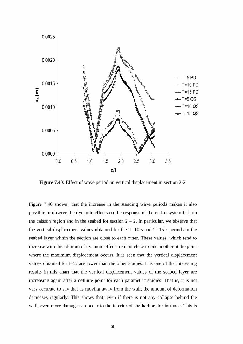
66
Figure 7.40: Effect of wave period on vertical displacement in section 2-2.
Figure 7.40 shows that the increase in the standing wave periods makes it also
possible to observe the dynamic effects on the response of the entire system in both
the caisson region and in the seabed for section 2 – 2. In particular, we observe that
the vertical displacement values obtained for the T=10 s and T=15 s periods in the
seabed layer within the section are close to each other. These values, which tend to
increase with the addition of dynamic effects remain close to one another at the point
where the maximum displacement occurs. It is seen that the vertical displacement
values obtained for t=5s are lower than the other studies. It is one of the interesting
results in this chart that the vertical displacement values of the seabed layer are
increasing again after a definite point for each parametric studies. That is, it is not
very accurate to say that as moving away from the wall, the amount of deformation
decreases regularly. This shows that; even if there is not any collapse behind the
wall, even more damage can occur to the interior of the harbor, for instance. This is
0.0000
0.0005
0.0010
0.0015
0.0020
0.0025
0.0 0.5 1.0 1.5 2.0 2.5 3.0 3.5
x/l
uz (m
)
T=5 PD
T=10 PD
T=15 PD
T=5 QS
T=10 QS
T=15 QS
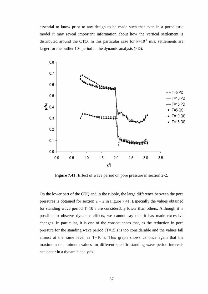
67
essential to know prior to any design to be made such that even in a poroelastic
model it may reveal important information about how the vertical settlement is
distributed around the CTQ. In this particular case for k=10-6
m/s, settlements are
larger for the outlier 10s period in the dynamic analysis (PD).
Figure 7.41: Effect of wave period on pore pressure in section 2-2.
On the lower part of the CTQ and in the rubble, the large difference between the pore
pressures is obtained for section 2 – 2 in Figure 7.41. Especially the values obtained
for standing wave period T=10 s are considerably lower than others. Although it is
possible to observe dynamic effects, we cannot say that it has made excessive
changes. In particular, it is one of the consequences that, as the reduction in pore
pressure for the standing wave period (T=15 s is too considerable and the values fall
almost at the same level as T=10 s. This graph shows us once again that the
maximum or minimum values for different specific standing wave period intervals
can occur in a dynamic analysis.
0.0
0.1
0.2
0.3
0.4
0.5
0.6
0.7
0.8
0.0 0.5 1.0 1.5 2.0 2.5 3.0 3.5
x/l
p/q
T=5 PD
T=10 PD
T=15 PD
T=5 QS
T=10 QS
T=15 QS
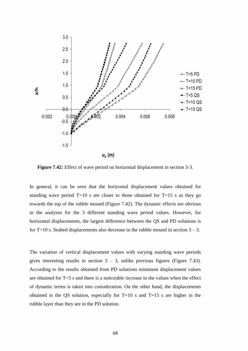
68
Figure 7.42: Effect of wave period on horizontal displacement in section 3-3.
In general, it can be seen that the horizontal displacement values obtained for
standing wave period T=10 s are closer to those obtained for T=15 s as they go
towards the top of the rubble mound (Figure 7.42). The dynamic effects are obvious
in the analyses for the 3 different standing wave period values. However, for
horizontal displacements, the largest difference between the QS and PD solutions is
for T=10 s. Seabed displacements also decrease in the rubble mound in section 3 – 3.
The variation of vertical displacement values with varying standing wave periods
gives interesting results in section 3 – 3, unlike previous figures (Figure 7.43).
According to the results obtained from PD solutions minimum displacement values
are obtained for T=5 s and there is a noticeable increase in the values when the effect
of dynamic terms is taken into consideration. On the other hand, the displacements
obtained in the QS solution, especially for T=10 s and T=15 s are higher in the
rubble layer than they are in the PD solution.
-1.5
-1.0
-0.5
0.0
0.5
1.0
1.5
2.0
2.5
3.0
-0.002 0.000 0.002 0.004 0.006 0.008
ux (m)
z/h
T=5 PD
T=10 PD
T=15 PD
T=5 QS
T=10 QS
T=15 QS
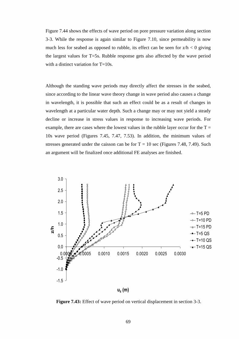
69
Figure 7.44 shows the effects of wave period on pore pressure variation along section
3-3. While the response is again similar to Figure 7.10, since permeability is now
much less for seabed as opposed to rubble, its effect can be seen for z/h < 0 giving
the largest values for T=5s. Rubble response gets also affected by the wave period
with a distinct variation for T=10s.
Although the standing wave periods may directly affect the stresses in the seabed,
since according to the linear wave theory change in wave period also causes a change
in wavelength, it is possible that such an effect could be as a result of changes in
wavelength at a particular water depth. Such a change may or may not yield a steady
decline or increase in stress values in response to increasing wave periods. For
example, there are cases where the lowest values in the rubble layer occur for the T =
10s wave period (Figures 7.45, 7.47, 7.53). In addition, the minimum values of
stresses generated under the caisson can be for T = 10 sec (Figures 7.48, 7.49). Such
an argument will be finalized once additional FE analyses are finished.
Figure 7.43: Effect of wave period on vertical displacement in section 3-3.
-1.5
-1.0
-0.5
0.0
0.5
1.0
1.5
2.0
2.5
3.0
0.0000 0.0005 0.0010 0.0015 0.0020 0.0025 0.0030
uz (m)
z/h
T=5 PD
T=10 PD
T=15 PD
T=5 QS
T=10 QS
T=15 QS
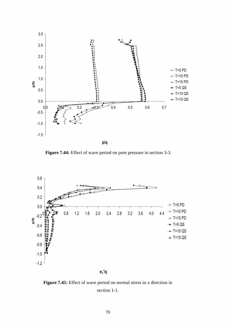
70
Figure 7.44: Effect of wave period on pore pressure in section 3-3.
Figure 7.45: Effect of wave period on normal stress in x direction in
section 1-1.
-1.5
-1.0
-0.5
0.0
0.5
1.0
1.5
2.0
2.5
3.0
0.0 0.1 0.2 0.3 0.4 0.5 0.6 0.7
p/q
z/h
T=5 PD
T=10 PD
T=15 PD
T=5 QS
T=10 QS
T=15 QS
-1.2
-1.0
-0.8
-0.6
-0.4
-0.2
0.0
0.2
0.4
0.6
0.0 0.4 0.8 1.2 1.6 2.0 2.4 2.8 3.2 3.6 4.0 4.4
σx'/q
z/h
T=5 PD
T=10 PD
T=15 PD
T=5 QS
T=10 QS
T=15 QS
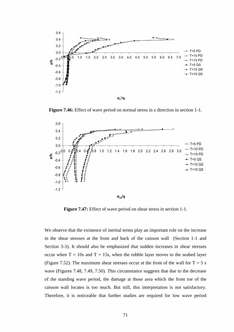
71
Figure 7.46: Effect of wave period on normal stress in z direction in section 1-1.
Figure 7.47: Effect of wave period on shear stress in section 1-1.
We observe that the existence of inertial terms play an important role on the increase
in the shear stresses at the front and back of the caisson wall (Section 1-1 and
Section 3-3). It should also be emphasized that sudden increases in shear stresses
occur when T = 10s and T = 15s, when the rubble layer moves to the seabed layer
(Figure 7.52). The maximum shear stresses occur at the front of the wall for T = 5 s
wave (Figures 7.48, 7.49, 7.50). This circumstance suggests that due to the decrease
of the standing wave period, the damage at those area which the front toe of the
caisson wall locates is too much. But still, this interpretation is not satisfactory.
Therefore, it is noticeable that further studies are required for low wave period
-1.2
-1.0
-0.8
-0.6
-0.4
-0.2
0.0
0.2
0.4
0.6
0.0 0.5 1.0 1.5 2.0 2.5 3.0 3.5 4.0 4.5 5.0 5.5 6.0 6.5 7.0
σz'/q
z/h
T=5 PD
T=10 PD
T=15 PD
T=5 QS
T=10 QS
T=15 QS
-1.2
-1.0
-0.8
-0.6
-0.4
-0.2
0.0
0.2
0.4
0.6
0.0 0.2 0.4 0.6 0.8 1.0 1.2 1.4 1.6 1.8 2.0 2.2 2.4 2.6 2.8 3.0
σxz/q
z/h
T=5 PD
T=10 PD
T=15 PD
T=5 QS
T=10 QS
T=15 QS

72
values. In some cases, as the wave periods increase, it is another important result that
the inertial terms lose their effect (Figure 7.51).
Figure 7.48: Effect of wave period on normal stress in x direction in section 2-2.
Figure 7.49: Effect of wave period on normal stress in z direction in section 2-2.
0.0
0.5
1.0
1.5
2.0
2.5
3.0
3.5
4.0
0.0 0.5 1.0 1.5 2.0 2.5 3.0 3.5
x/l
σx'/q
T=5 PD
T=10 PD
T=15 PD
T=5 QS
T=10 QS
T=15 QS
0
1
2
3
4
5
6
0.0 0.5 1.0 1.5 2.0 2.5 3.0 3.5
x/l
σz'/q
T=5 PD
T=10 PD
T=15 PD
T=5 QS
T=10 QS
T=15 QS
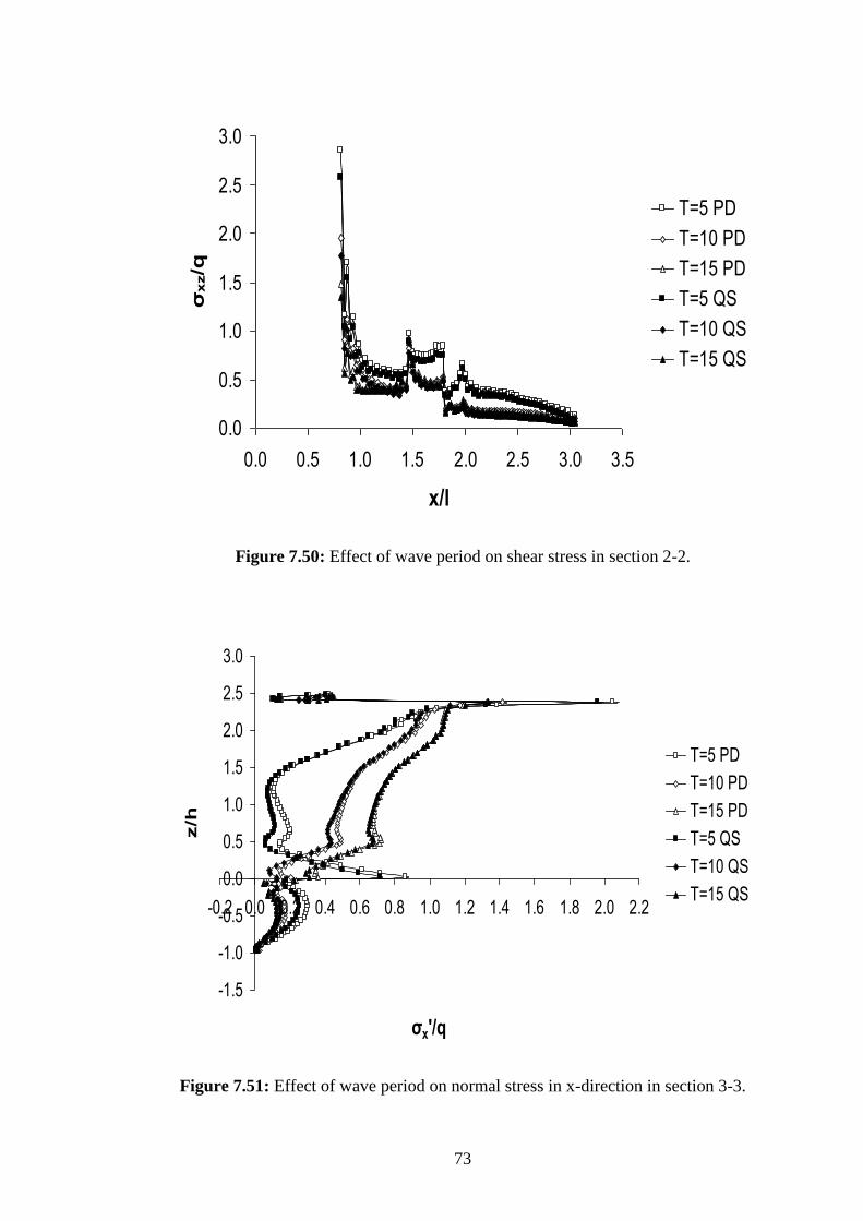
73
Figure 7.50: Effect of wave period on shear stress in section 2-2.
Figure 7.51: Effect of wave period on normal stress in x-direction in section 3-3.
0.0
0.5
1.0
1.5
2.0
2.5
3.0
0.0 0.5 1.0 1.5 2.0 2.5 3.0 3.5
x/l
σx
z/q
T=5 PD
T=10 PD
T=15 PD
T=5 QS
T=10 QS
T=15 QS
-1.5
-1.0
-0.5
0.0
0.5
1.0
1.5
2.0
2.5
3.0
-0.2 0.0 0.2 0.4 0.6 0.8 1.0 1.2 1.4 1.6 1.8 2.0 2.2
σx'/q
z/h
T=5 PD
T=10 PD
T=15 PD
T=5 QS
T=10 QS
T=15 QS
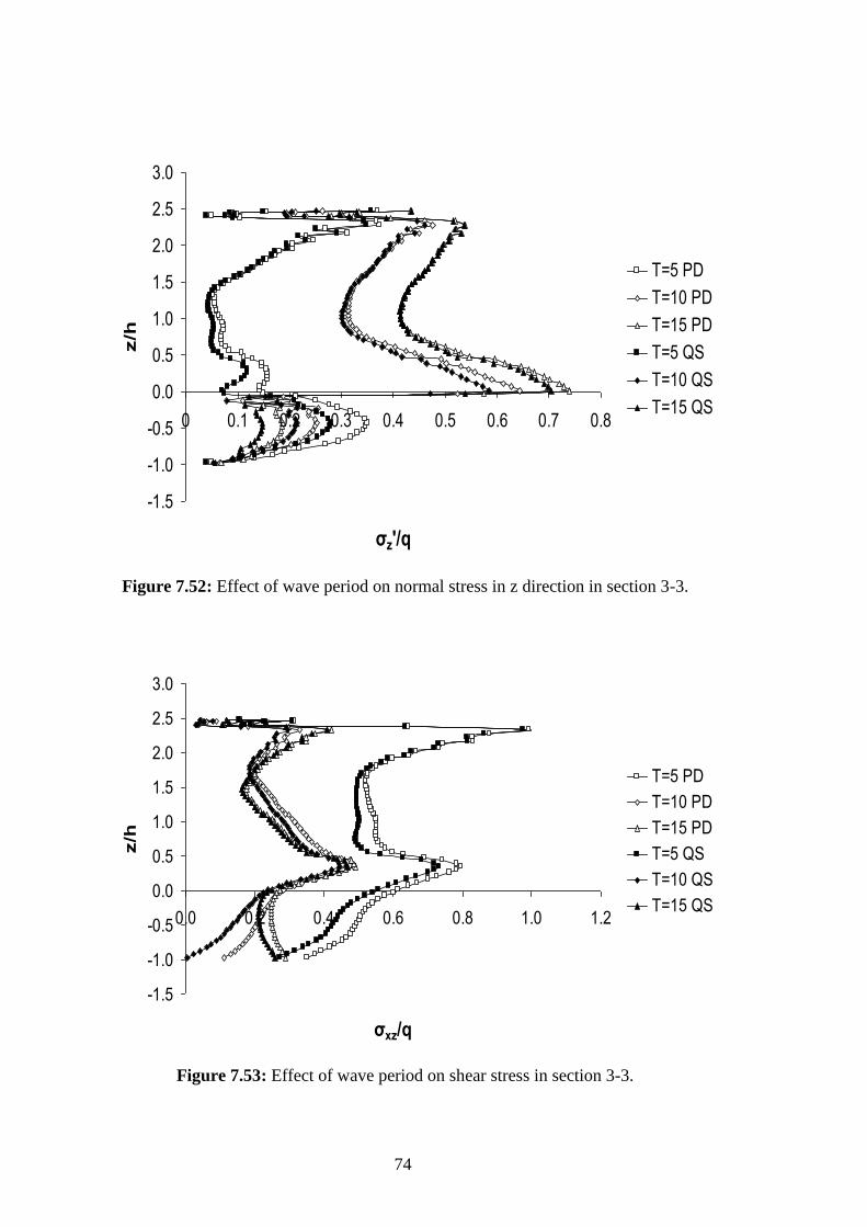
74
Figure 7.52: Effect of wave period on normal stress in z direction in section 3-3.
Figure 7.53: Effect of wave period on shear stress in section 3-3.
-1.5
-1.0
-0.5
0.0
0.5
1.0
1.5
2.0
2.5
3.0
0 0.1 0.2 0.3 0.4 0.5 0.6 0.7 0.8
σz'/q
z/h
T=5 PD
T=10 PD
T=15 PD
T=5 QS
T=10 QS
T=15 QS
-1.5
-1.0
-0.5
0.0
0.5
1.0
1.5
2.0
2.5
3.0
0.0 0.2 0.4 0.6 0.8 1.0 1.2
σxz/q
z/h
T=5 PD
T=10 PD
T=15 PD
T=5 QS
T=10 QS
T=15 QS
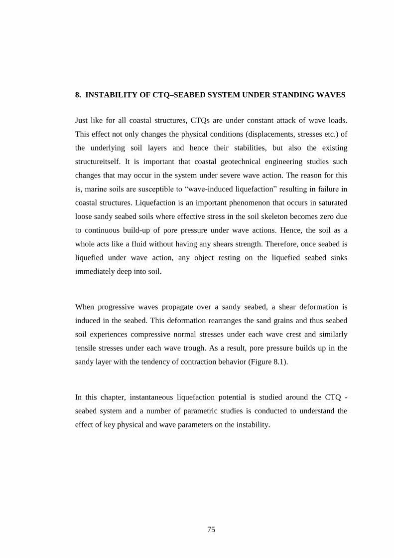
75
8. INSTABILITY OF CTQ–SEABED SYSTEM UNDER STANDING WAVES
Just like for all coastal structures, CTQs are under constant attack of wave loads.
This effect not only changes the physical conditions (displacements, stresses etc.) of
the underlying soil layers and hence their stabilities, but also the existing
structureitself. It is important that coastal geotechnical engineering studies such
changes that may occur in the system under severe wave action. The reason for this
is, marine soils are susceptible to “wave-induced liquefaction” resulting in failure in
coastal structures. Liquefaction is an important phenomenon that occurs in saturated
loose sandy seabed soils where effective stress in the soil skeleton becomes zero due
to continuous build-up of pore pressure under wave actions. Hence, the soil as a
whole acts like a fluid without having any shears strength. Therefore, once seabed is
liquefied under wave action, any object resting on the liquefied seabed sinks
immediately deep into soil.
When progressive waves propagate over a sandy seabed, a shear deformation is
induced in the seabed. This deformation rearranges the sand grains and thus seabed
soil experiences compressive normal stresses under each wave crest and similarly
tensile stresses under each wave trough. As a result, pore pressure builds up in the
sandy layer with the tendency of contraction behavior (Figure 8.1).
In this chapter, instantaneous liquefaction potential is studied around the CTQ -
seabed system and a number of parametric studies is conducted to understand the
effect of key physical and wave parameters on the instability.
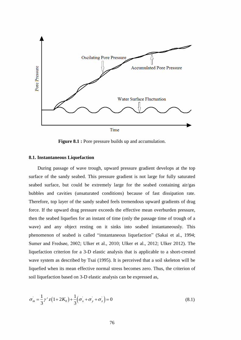
76
Figure 8.1 : Pore pressure builds up and accumulation.
8.1. Instantaneous Liquefaction
During passage of wave trough, upward pressure gradient develops at the top
surface of the sandy seabed. This pressure gradient is not large for fully saturated
seabed surface, but could be extremely large for the seabed containing air/gas
bubbles and cavities (unsaturated conditions) because of fast dissipation rate.
Therefore, top layer of the sandy seabed feels tremendous upward gradients of drag
force. If the upward drag pressure exceeds the effective mean overburden pressure,
then the seabed liquefies for an instant of time (only the passage time of trough of a
wave) and any object resting on it sinks into seabed instantaneously. This
phenomenon of seabed is called “instantaneous liquefaction” (Sakai et al., 1994;
Sumer and Fredsøe, 2002; Ulker et al., 2010; Ulker et al., 2012; Ulker 2012). The
liquefaction criterion for a 3-D elastic analysis that is applicable to a short-crested
wave system as described by Tsai (1995). It is perceived that a soil skeleton will be
liquefied when its mean effective normal stress becomes zero. Thus, the criterion of
soil liquefaction based on 3-D elastic analysis can be expressed as,
0
1 11 2 0
3 3
' ' ' 'm x y z' z K
(8.1)
77
where K0 is the coefficient of lateral earth pressure at rest and ' ' 'x y z
is the
sum of normal effective stresses induced by wave on the sea floor. Elastic
equilibrium requires,
01
K
(8.2)
where is the Poisson‟s ratio. If we write ' ' 'y x z for plane strain, the
relation (5.4) is written as,
0
11 2 1 0
3
' ' 'm x z' z K
(8.3)
In this study, the comparison of the instability of seabed is made with the
available results in the literature for a seabed layer based on the effective mean stress
criterion described in (8.3) to predict the region of instantaneous liquefaction. Then
the actual seabed instability around and underneath the caisson is evaluated based on
the total (i.e. including the in-situ effective mean stress of soil) effective mean
stresses in the seabed due to wave-action are calculated. This criterion simply states
that when the effective mean normal stress in the seabed under wave load becomes
zero, the soil liquefies. Most of the time seabed will have some air in its voids due to
deposition characteristics as well as grain size distribution but there are some studies
that suggest that some air/gas may also be produced by marine micro-organisms in
the seabed such as bacteria (Sumer and Fredsøe, 2002). It should be noted here that
instantaneous liquefaction occurs even if there is not permanent deformations in the
soil. That is, pore water pressure oscillates in time (either harmonically or in the case
of irregular waves following closely the induced wave pattern) without any
accumulation essentially carried by pore water. However, in order for instantaneous
liquefaction to exist, there must be some air present in the voids of the porous seabed
such that any upward gradient of induced wave motion will not be balanced by
gradual rise of corresponding pore pressure but it will basically overcome the
effective stress of the soil. Therefore degree of saturation, S<1 must hold. When that
happens, the soil cannot resist the tension induced by wave trough and the soil
78
liquefies. In this chapter, the potential of instantaneous liquefaction is investigated
through FE analyses for the CTQ – seabed system.
Figure 8.2: Instantaneous liquefaction caused by waves (after de Groot et al., 2006)
8.2 Numerical Analysis of Liquefaction
Numerical results are obtained by using the FEM the basics of which are outlined in
Chapter 4. Plane-strain analyses are performed and the linear elastic behavior for the
deformation of the soil skeleton and the quay wall is assumed. The FE model of the
CTQ-seabed-rubble system is same as the one used previously for the standing wave
action. The QS and PD formulations require the horizontal and vertical
displacements, xu and zu and the pressure, p specified as DOFs at the nodal points.
However, now the numerical aspects of the FE analyses in terms of the duration and
time history of loads as well as output parameters are different. In the case of wave-
induced hydrodynamic pressures caused by standing wave loads, the seabed and
rubble boundary is under hydrostatic wave load followed by standing pressures
(Figure 8.3). The standing wave amplitude, 0q and wave pressure, p are calculated
as:
).cosh(20
dk
gHq w (8.1)
)cos()cos()cosh(+= 0 wtkxkzqdγp w (8.2)
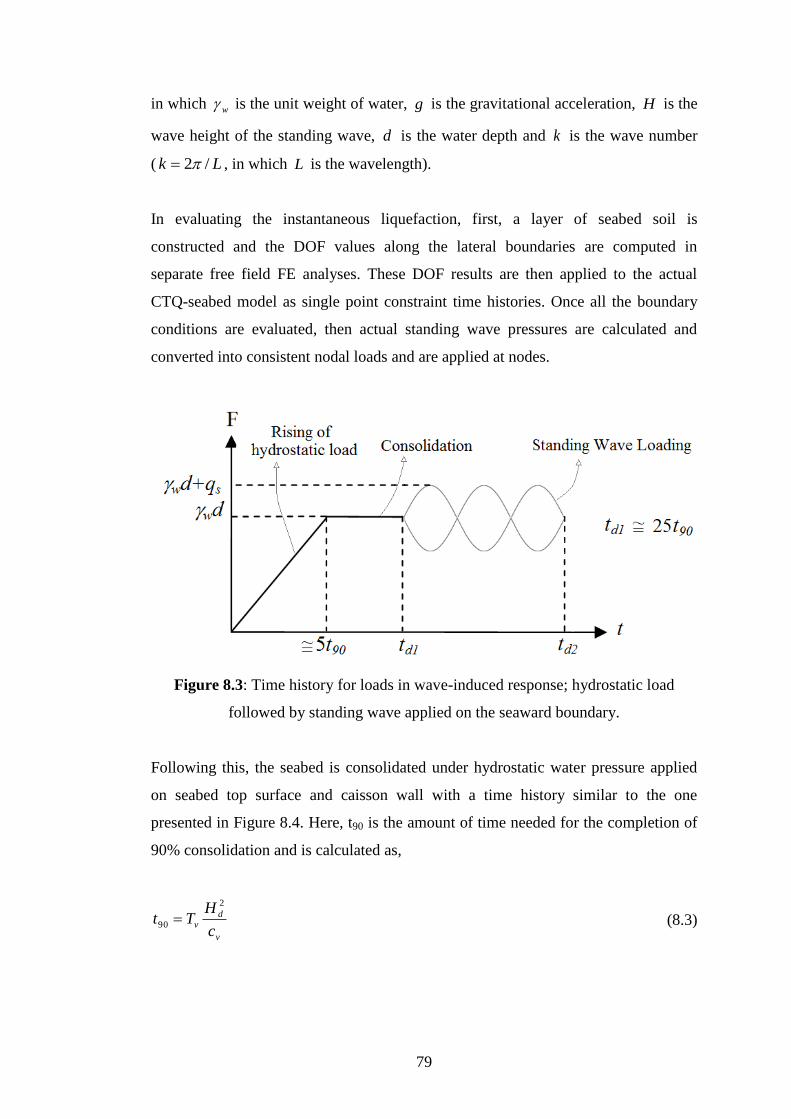
79
in which w is the unit weight of water, g is the gravitational acceleration, H is the
wave height of the standing wave, d is the water depth and k is the wave number
( Lk /2 , in which L is the wavelength).
In evaluating the instantaneous liquefaction, first, a layer of seabed soil is
constructed and the DOF values along the lateral boundaries are computed in
separate free field FE analyses. These DOF results are then applied to the actual
CTQ-seabed model as single point constraint time histories. Once all the boundary
conditions are evaluated, then actual standing wave pressures are calculated and
converted into consistent nodal loads and are applied at nodes.
Figure 8.3: Time history for loads in wave-induced response; hydrostatic load
followed by standing wave applied on the seaward boundary.
Following this, the seabed is consolidated under hydrostatic water pressure applied
on seabed top surface and caisson wall with a time history similar to the one
presented in Figure 8.4. Here, t90 is the amount of time needed for the completion of
90% consolidation and is calculated as,
v
d
vc
HTt
2
90 (8.3)
80
where cv is the consolidation coefficient, Hd is the drainage distance of the layer and
the time factor, Tv, is 0.848 corresponding to 90% consolidation. The consolidation
coefficient, cv is calculated from,
wv
zv
m
kc
(8.4)
where kz is the vertical permeability, w is the unit weight of water and vm is the
volumetric compressibility coefficient and is found from,
)1(2
21
Gmv (8.5)
where G is the shear modulus. The pore pressure values in the soil layer are
dissipated imitating the condition actualising in the field by taking rise time of about
4-5 times the t90. Hydrodynamic wave loads caused by standing waves for the cyclic
response of seabed are applied to the seaward boundary after the completion of
consolidation under hydrostatic pressure. The dynamic response of the system is
attained until arriving steady state (Ulker, 2009).
8.3 Parametric Study Results
In this section, the results of a parametric study investigating the effect of some key
wave and seabed parameters to the standing wave-induced liquefaction potential are
presented. The results are presented in terms of the contour plots of effective mean
normal stresses (Sm, '
m ) inside the domain. This way it is possible to identify the
regions where it becomes zero, hence the instantaneous liquefaction. The analyses
were carried out by using QS formulation where all the inertial terms are neglected
and by PD formulation where only the inertial terms associated with the relative pore
fluid displacement are excluded to examine the effect of the inertial terms on the
instantaneous liquefaction. In addition, S 0.999 is chosen for Kf=2GPa to identify
the locations that may possibly liquefy even for a very small unsaturation.
81
8.3.1 Effect of seabed permeability
When the form of the system is evaluated by permeability changes, the first thing to
notice is that the width of the instantaneous liquefaction area, including the seabed-
landfill layers, locates at the back of the caisson type quay wall for k=10-4
m/s
(Figure 8.6). The upper half of the seabed layer and fill just above it reaches positive
Sm values together. This indicates that there is instantaneous liquefaction in the
region. We see that instantaneous liquefaction values do not show a direct or inverse
proportion with seabed permeability, because the widest liquefactive zones are
obtained for k=10E-4 m/s. However, since the rocking effect is somewhat greater for
the k=10E-6 m/s study, the maximum Sm value is obtained in the rubble mound layer
of the front toe region of the CTQ (Figure 8.8). Accordingly, an increase in the
liquefied area is observed due to accumulation of tensile stresses during the wave
motion behind the caisson in the upper part of the the fill. Results obtained according
to all three different permeability values indicate that the inertial terms have
negligible effect for reaching instantaneous liquefaction potential at the bottom of the
caisson, system-wide. This does not apply to the back top of the CTQ. The presence
of dynamic effects has greatly expanded the area of instantaneous liquefaction in this
zone (Figures 8.5-8.6-8.8).
8.3.2 Effect of seabed soil type
We see a concentration of instantaneous liquefaction zones at seabed layer below the
rubble (Figure 8.7). This, however, is not a result observed in this region in other
cases. The poor grading of the soil is a triggering factor for reaching the positive
pressure values. The main result of the other graphs is also seen here; the upper
corner of the seabed layer under the sea has undergone instantaneous liquefaction. In
addition, we can see this result for all seabed surfaces. It is possible to say that the
rocking effect is lower for GW, which has a smaller amount of void space because of
its well gradation in comparison to GP or GM. At the back of the caisson, there is
some considerable liquefaction in the alluvial clay layer (Figure 8.9).
82
8.3.3 Effect of standing wave period
There is no significant effect of the wave period change on the instantaneous
liquefaction potential, except for a few small locations in the seabed under the rubble
and in the upper small area of the rubble mound (Figures 8.4, 8.8 and 8.10).
However, some results indicate that for the period of T = 15 s, the PD solution result
in the areas where negative pressure values are obtained in the back toe of the rubble
mound in a decreasing manner and accordingly the instantaneous liquefaction
behavior increases in the landfill layer. Some liquefaction response is also observed
in the seabed layer behind the caisson (Figure 8.10).
8.4 Shear Stress Variations
In this study, the actual variations of shear stresses as developed along the cross
sections of concerns are also computed. These are plotted in terms of their contours
across the entire problem domain (i.e. CTQ-seabed-backfill). What we mean by
“actual shear” here is that the shear stresses are calculated in this section while
considering the body forces (i.e. weights) as well as the hydrostatic and more
importantly hydrodynamic standing wave forces acting at the surface of the domain.
Therefore, such calculations of the shear stresses are more realistic as opposed to the
“excess” values where no body forces or hydrostatic forces are included. In the
below, effects of seabed permeability, the soil type and the wave period on the
variations of shear stresses are briefly presented. This way, it is possible to identify
the locations of high shear concentrations that may possibly lead to shear failure
around the CTQ in the soil.
8.4.1 Effect of seabed permeability
We note that there is some increase in shear stresses obtained in the seabed layer
below the caisson corresponding to some decrease in permeability. Excessive water
flow in the seabed somewhat reduces the soil shear resistance. The result we have
obtained confirms this. It can be also said that the values obtained in PD solutions are
slightly lower than QS. With the study of inertial terms, it can be thought that the
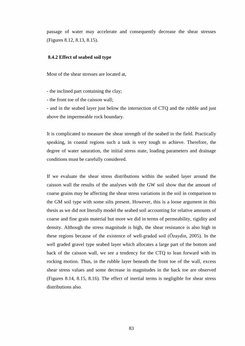
83
passage of water may accelerate and consequently decrease the shear stresses
(Figures 8.12, 8.13, 8.15).
8.4.2 Effect of seabed soil type
Most of the shear stresses are located at,
- the inclined part containing the clay;
- the front toe of the caisson wall;
- and in the seabed layer just below the intersection of CTQ and the rubble and just
above the impermeable rock boundary.
It is complicated to measure the shear strength of the seabed in the field. Practically
speaking, in coastal regions such a task is very tough to achieve. Therefore, the
degree of water saturation, the initial stress state, loading parameters and drainage
conditions must be carefully considered.
If we evaluate the shear stress distributions within the seabed layer around the
caisson wall the results of the analyses with the GW soil show that the amount of
coarse grains may be affecting the shear stress variations in the soil in comparison to
the GM soil type with some silts present. However, this is a loose argument in this
thesis as we did not literally model the seabed soil accounting for relative amounts of
coarse and fine grain material but more we did in terms of permeability, rigidity and
density. Although the stress magnitude is high, the shear resistance is also high in
these regions because of the existence of well-graded soil (Özaydin, 2005). In the
well graded gravel type seabed layer which allocates a large part of the bottom and
back of the caisson wall, we see a tendency for the CTQ to lean forward with its
rocking motion. Thus, in the rubble layer beneath the front toe of the wall, excess
shear stress values and some decrease in magnitudes in the back toe are observed
(Figures 8.14, 8.15, 8.16). The effect of inertial terms is negligible for shear stress
distributions also.
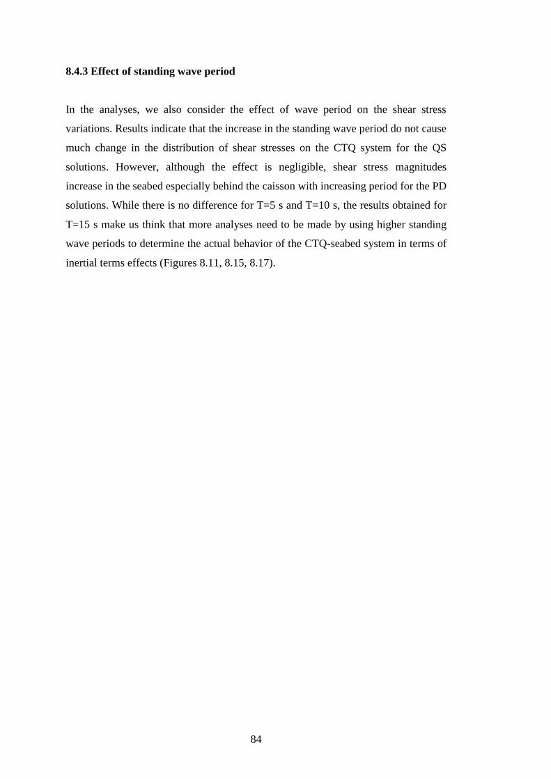
84
8.4.3 Effect of standing wave period
In the analyses, we also consider the effect of wave period on the shear stress
variations. Results indicate that the increase in the standing wave period do not cause
much change in the distribution of shear stresses on the CTQ system for the QS
solutions. However, although the effect is negligible, shear stress magnitudes
increase in the seabed especially behind the caisson with increasing period for the PD
solutions. While there is no difference for T=5 s and T=10 s, the results obtained for
T=15 s make us think that more analyses need to be made by using higher standing
wave periods to determine the actual behavior of the CTQ-seabed system in terms of
inertial terms effects (Figures 8.11, 8.15, 8.17).
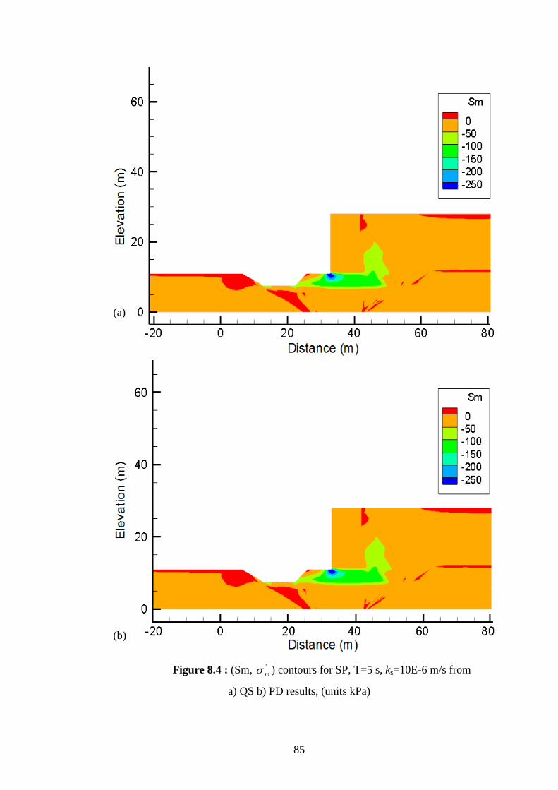
85
Figure 8.4 : (Sm, '
m ) contours for SP, T=5 s, ks=10E-6 m/s from
a) QS b) PD results, (units kPa)
(a)
(b)
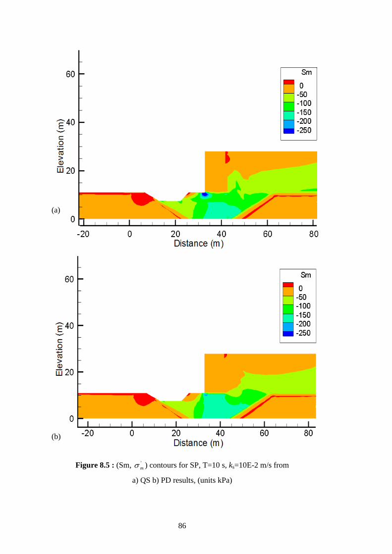
86
Figure 8.5 : (Sm, '
m ) contours for SP, T=10 s, ks=10E-2 m/s from
a) QS b) PD results, (units kPa)
(a)
(b)
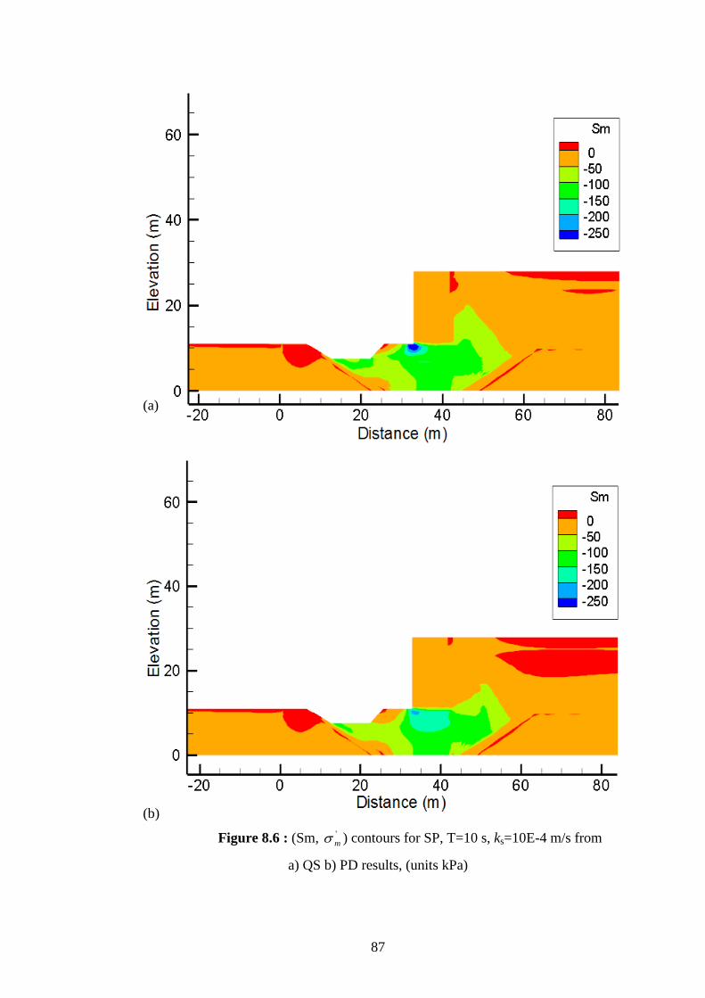
87
Figure 8.6 : (Sm, '
m ) contours for SP, T=10 s, ks=10E-4 m/s from
a) QS b) PD results, (units kPa)
(a)
(b)
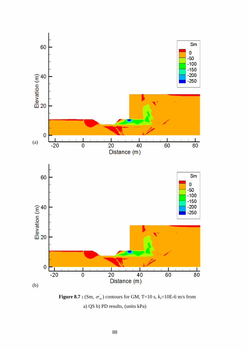
88
Figure 8.7 : (Sm, '
m ) contours for GM, T=10 s, ks=10E-6 m/s from
a) QS b) PD results, (units kPa)
(a)
(b)
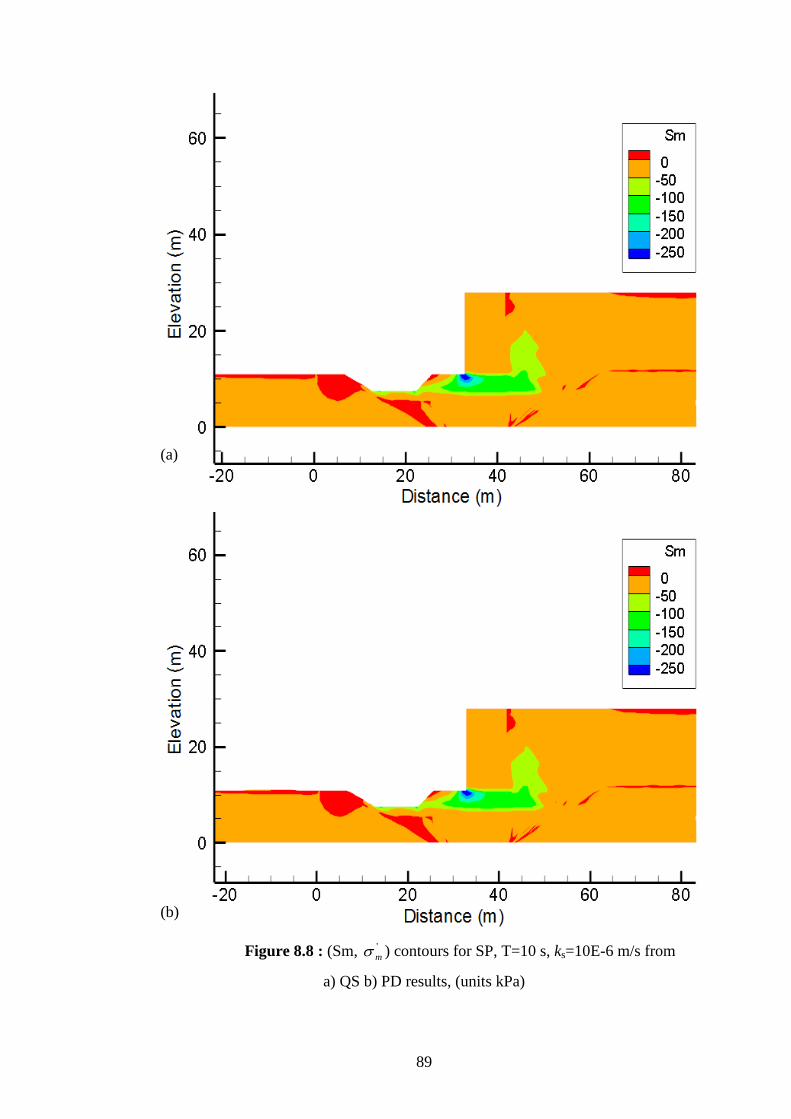
89
Figure 8.8 : (Sm, '
m ) contours for SP, T=10 s, ks=10E-6 m/s from
a) QS b) PD results, (units kPa)
(a)
(b)
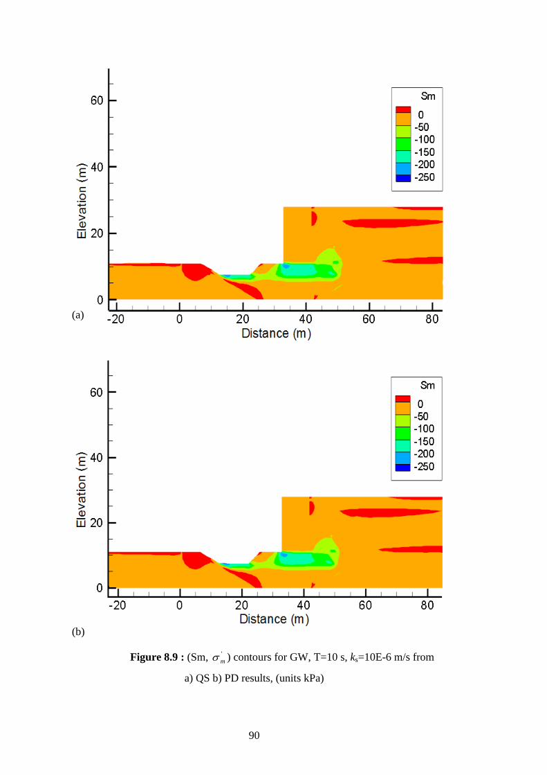
90
Figure 8.9 : (Sm, '
m ) contours for GW, T=10 s, ks=10E-6 m/s from
a) QS b) PD results, (units kPa)
(a)
(b)
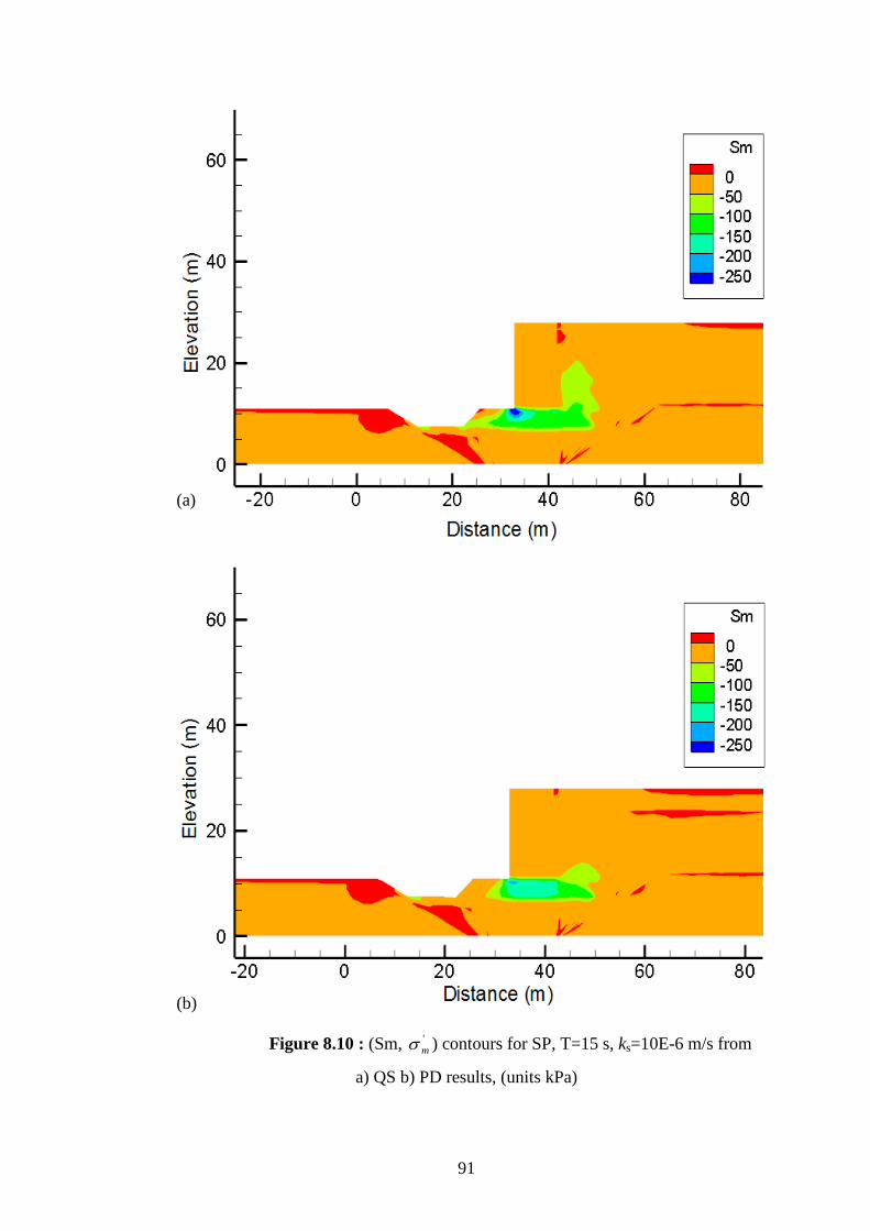
91
Figure 8.10 : (Sm, '
m ) contours for SP, T=15 s, ks=10E-6 m/s from
a) QS b) PD results, (units kPa)
(a)
(b)
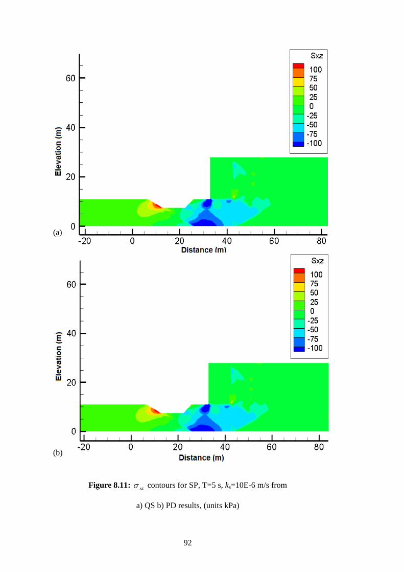
92
Figure 8.11: xz contours for SP, T=5 s, ks=10E-6 m/s from
a) QS b) PD results, (units kPa)
(a)
(b)
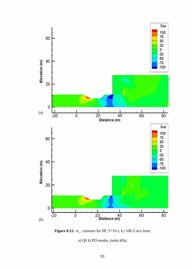
93
Figure 8.12: xz contours for SP, T=10 s, ks=10E-2 m/s from
a) QS b) PD results, (units kPa)
(a)
(b)
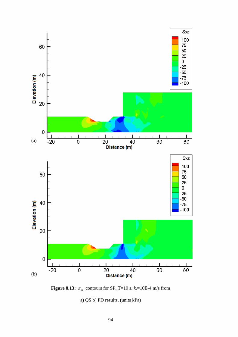
94
Figure 8.13: xz contours for SP, T=10 s, ks=10E-4 m/s from
a) QS b) PD results, (units kPa)
(a)
(b)
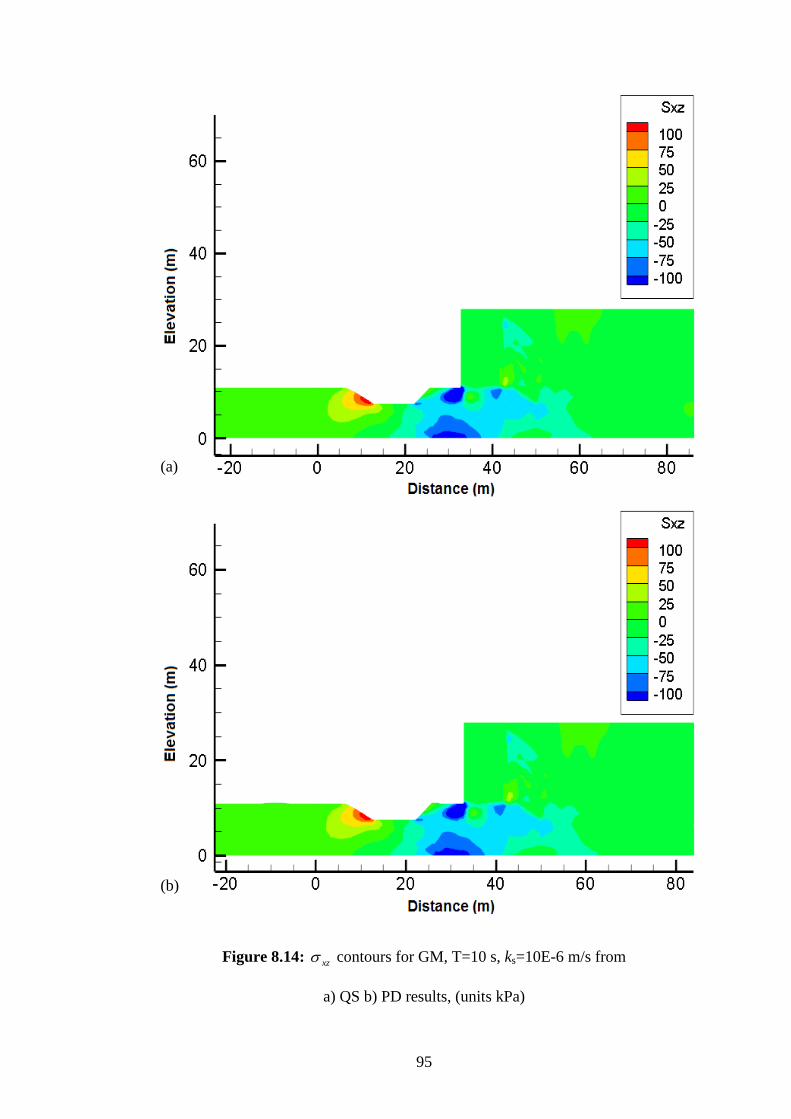
95
Figure 8.14: xz contours for GM, T=10 s, ks=10E-6 m/s from
a) QS b) PD results, (units kPa)
(a)
(b)

96
Figure 8.15: xz contours for SP, T=10 s, ks=10E-6 m/s from
a) QS b) PD results, (units kPa)
(a)
(b)
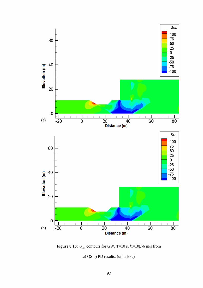
97
Figure 8.16: xz contours for GW, T=10 s, ks=10E-6 m/s from
a) QS b) PD results, (units kPa)
(a)
(b)
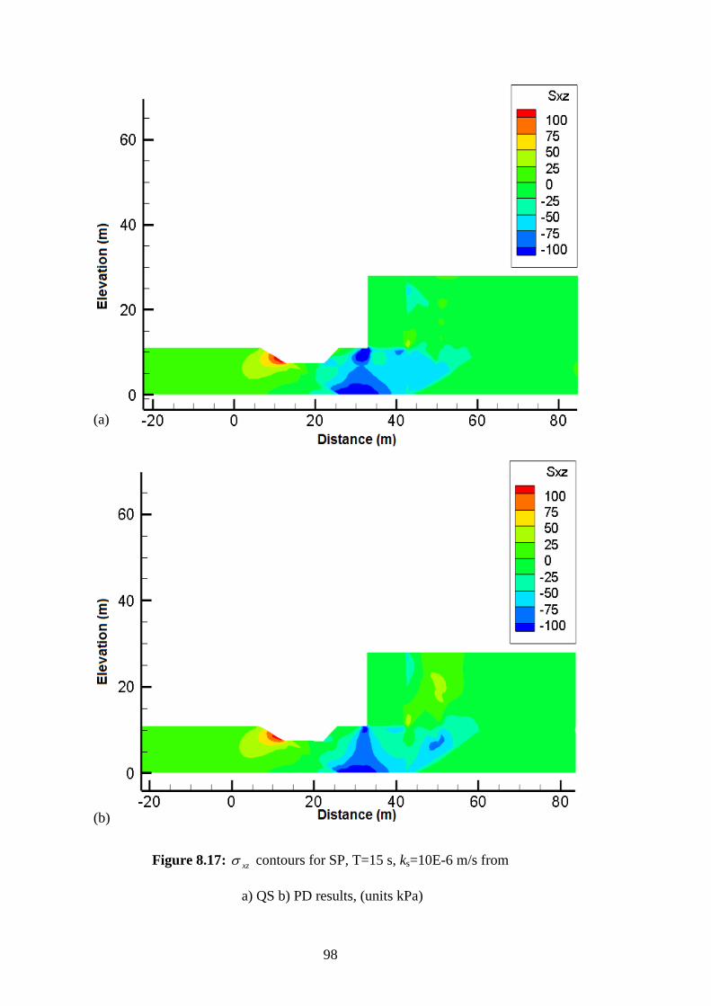
98
Figure 8.17: xz contours for SP, T=15 s, ks=10E-6 m/s from
a) QS b) PD results, (units kPa)
(a)
(b)

99
9. CONCLUSIONS
In this study, dynamic response and instability of a caisson type quay wall (CTQ)-
seabed-backfill system is modeled against standing wave action. The CTQ studied
actually exist in reality and the one that experienced some damage at the Kobe Port
in Japan was selected as a case study. Although it is not a common practice to
evaluate the dynamic response of quay walls under severe wave conditions as more
often than not breakwaters are built to protect such structures and the communities
behind, sometimes that is not the case as in the case of Ambarli port in Istanbul and
hence, it makes conducting such analyses a requirement for researchers. That is why
we have carried out a set of parametric studies for understanding the factors
contributing to the actual dynamic response of an existing CTQ under standing
waves. So we believe that this study has some merit in the state-of-the-art of coastal
geotechnical engineering in that regards.
In our model, CTQ is assumed to behave linear elastically and the seabed soil, the
backfilland the rubble are all modeled using the poroelastic formulation developed
by Biot in terms of the theory of coupled flow and deformation. The mathematical
formulation is first written in terms of the governing partial differential equations
considering the physical laws behind. Then they are combined to give the final forms
in terms of the degrees of freedom of the soil, in this case solid grain displacement
and pore water pressure, by neglecting the inertial terms associated with the relative
motion of pore water. This leads to the simplified formulations namely the partially
dynamic (PD) and the quasi-static forms (QS). These two formulations were used
throughout this thesis in the numerical analyses. Classical finite elements are used to
discretize the governing equations and dynamic analyses are carried out in time
domain until the system has reached steady state response. We, then, focus our
attention on the vertical displacements, pore water pressure and shear stress
variations in time and 2-D space in the CTQ-seabed-rubble system. Their variations
100
in temporal and spatial domains are evaluated for changing seabed permeability and
wave period. These are the key parameters chosen here to study the system behavior.
Other important soil and wave parameters such as soil rigidity and the wavelength
are of part of an ongoing study.
Based on the results of our study, we find that response parameters mostly increase
in magnitude particularly in the rubble as the permeability of the seabed decreases.
However, for varying values of wave period, the picture is not that clear and may
sometimed yield unexpected behavior as T=10s wave yields as an outlier among
others. For example, in some cases it gives the largest vertical displacements. While
our work continues in comparing the response with that of the one around the natural
period of the combined wall-seabed-rubble system, provided that we know the
natural period, it seems that further analyses are required around close proximity of
10s wave. It should also be noted that as the quay wall does its rocking motion under
incoming waves, it actually transfers its movement into the stiff rubble backfill
behind it which results in significant stress concentrations not just at the toes of the
caisson but at the interface between the rubble and the seabed as well. Also, sudden
pore pressure dissipations in the seabed, seemingly an interesting result of this study,
might be associated with this behavior as there is surely many locations in the seabed
where more drained conditions than others exist along the cross sections of interest
which are the vertical sections in front of and behind the caisson and a horizontal
section underneath it along the interface between the caisson and the rubble.
Instability of the CTQ-seabed system is also studied. For that, standing wave-induced
instantaneous liquefaction potential inside the soil around the CTQ is considered.
Liquefaction is observed not only at the upper corners of the clay soil and the rubble,
but also around the boundaries of the clay layer and the seabed and backfill soil of
the CTQ. In general, the liquefaction results are intriguing for k=10E-4 m/s seabed
permeabilityin areas close to the seabed surface andbehind the wall. It is also worth
mentioning that inertial terms assocaited with the solid motion are not of a major
effect on the liquefaction potential of the whole system. Last but not least, the next
section summarizes the ongoing study.
101
10. FUTURE WORKS
Standing wave-induced CTQ-seabed system response is studied in details
considering key wave and soil parameters determining the dynamic response of the
system. Moreover, instability analyses are made to determine the liquefaction
potential. Adding material nonlinearity to FE analyses, further research will be done
to draw a complete picture of the actual observed liquefaction behavior of seabed as
well as permanent deformations of the soil leading potentially to the failure of the
CTQ. Here the liquefaction behavior of seabed is the liquefaction caused by
progressive build-up of pore pressure due to cyclic shear stresses under wave
loading. Another work to be investigated further is the use of the linear wave theory,
to identify exactly what seabed parameter (wavelength of wave period) is causing the
real effect on the response in the dynamic analyses. Since the period increment
means increasing the wavelength value also and there is a need to do more research
on how this affects DOF‟s exactly. In addition, the response spectrum can be
obtained by analyzing under the effects of variable standing wave period values in
subsequent studies.

102
103
REFERENCES
Alyami, M., Wilkinson S.M., Rouainia, M. and Cai, F. (2007), “Simulation of
Seismic Behaviour of Gravity Quay Wall Using a Generalized
Plasticity Model”, Pros. of the 4th
Int. Conf. on Earthquake
Geotechnical Engineering, Thessaloniki, Greece.
Biot, M.A. (1941). “General Theory of Three Dimensional Consolidation”, J Applied
Physics, 12, 155-164.
Biot, M.A. (1955). “Theory of Elasticity and Consolidation for a Porous Anisotropic
Solid”, J Applied Physics, 26, 182-185.
Biot, M.A. (1962). “Generalized Theory of Acoustic Propagation in Porous
Dissipative Media”, J Acoustical Society of America, 34(5), 1254-
1264.
Cheng, A.H.D. (2016), “Poroelasticity”, Vol. 27. Springer.
Cook, R.D., Malkus, D.S., Plesha, M.E. and Witt, R.J. (2001), “SConcepts and
applications of finite element analysis”, Fourth Edition, John Wiley
and Sons, New York.
Dakoulas, P. and Gazetas, G. (2005), “Seismic effective-stress analysis of cassion
quay walls: Application to Kobe”, Journal of Soils and Foundations,
45, 133-147.
De Gijt, J. G., and Broeken, M. L. (2005), “Handbook of Quay Walls”, CRC Press.
De Groot, M.B., Bolton, M.D., Foray, P., Meijers, P., Palmer, A.C., Sandven,
R., Sawicki, A. and Teh, T.C. (2006), “Physics of Liquefaction
Phenomena under marine structures”, Journal of Waterway, Port,
Coastal and Ocean Engineering, ASCE Vol.132, No.4, 227-243.
Dean, R. G., and Dalrymple, R. A. (1991). “Water wave mechanics for engineers
and scientists”, World Scientific Publishing Co Inc. Vol.2 p.58
Detournay, E. and Cheng, A. H. D. (1993), “Fundamentals of poroelasticity,
comprehensive rock engineering: principles, practice and projects.
Analysis and design method”.
El-Sharnouby, B., El-Kamhawy, H., and Al-Yami, M. (2004), “Analysis of
gravity quay walls”, Alexandria Engineering Journal, 43(5), 663-669.

104
George, N. (2007), “Quays Impacted by Strong Waves and Ways of Strengthening
Old Quays Damaged by Waves or from Propeller Induced Scours”,
Doctoral Dissertation, Tei Piraeus – Kingston University, Athens,
Greece.
Guddati, M. N., Savadatti, S., Ulker, M.B.C., Thirunavukkarasu, S., (2009),
“FIONA 3D: A General Purpose Object – Oriented Nonlinear Finite
Element Program in C++”, North Carolina State University, Raleigh,
NC, USA.
Gumucio, J. L. (2013), “Design of Quay Walls using the Finite Element Method”.
Master Thesis, Technische Universiteit Delft, Rotterdam, Nederland.
Iai, S. (2011), “Seismic Performance of Port Structures: Assessment and
Remediation”, 7th
National Conference on Earthquake Engineering,
Istanbul, Turkey.
Iai, S. (1998), “Seismic analysis and performance of retaining structures”,
Proceedings of the 1998. Conference on Geotechnical Earthquake
Engineering and Soil Dynamics III, Part 2 (of 2), ASCE, 1020-1044,
1998.
Inagaki, H., Iai, S., Sugano, T., Yamazaki, H. and Inatomi, T. (1996),
“Performance of cassion type quay walls at Kope Port”, Special issue
of soils and foundations, 119-136.
Karakus, H. (2007), “New seismic design approaches for block type quay walls”,
Master Thesis, Middle East Technical University, Ankara, Turkey.
Khan-Mozahedy, A. B. M. (2015), “Subsidence phenomena of the coastal structures
into offshore sandy seabed: a review”. Int. J. Sci. Eng. Res., 6(7),
1600-1611.
Kirca, V. S. O., Sumer, B. M. and Fredsøe, J. (2013), “Residual liquefaction of
seabed under standing waves”. Journal of Waterway, Port, Coastal,
and Ocean Engineering, 139(6), 489-501.
Kudella, M., Oumeraci, H., De Groot., M.B. and Meijers, P. (2006), “Large-Scale
Experiments on Pore Pressure Generation Underneath a Caisson
Breakwater”, J Waterway, Port, Coast. Ocean Engineering, ASCE
132(4), 310-324.
Liquefaction and Ports: Kobe. (2017), Retrieved April 22, 2017, from
https://research.engineering.ucdavis.edu/gpa/earthquakehazards/liqu
efaction-ports “Civil and Environmental Engineering”, University of
California.
Liu, X. (2008), “Numerical models for scour and liquefaction around object under
currents and waves”, Doctoral Dissertation, University of Illinois,
Urbana-Champaign, USA.
105
Lundgren, H., Lindhardt Jacobsen, H.C., Romhild, C.J., (1989), “Stability of
breakwaters on porous foundations”. In: Proceedings of the 12th
International Conference on Soil Mechanics and Foundation
Engineering, pp. 451–454.
Maeno, S., and Nago, H. (1988), “Settlement of a concrete block into a sand bed
under water pressure variation”. In Proceedings of the International
Symposium on Modelling Soil-Water-Structure Interactions (pp.67-
76).
Mase, H., Sakai, T. and Sakamoto, M., (1994), “Wave-induced pore water
pressures and effective stresses around breakwater”. Ocean
Engineering 21 (4), 361–379.
Okusa, S. (1985), “Wave induced stresses in unsaturated submarine sediments”,
Geotechnique 35 (4), 517–532.
Ozaydin, K. (2005). “Soil Mechanics”,. Birsen Publishing, İstanbul. p 203 (in
Turkish).
Port of Kobe. (2010), Retrieved April 22, 2017, from http://www.city.kobe.lg.jp/life/
access/harbor/english/shisetsu_e.html “City of Kobe”, United Nations
Educational, Scientific and Cultural Organization, Kobe City, Japan.
Rendulic, L. (1936), “Relation between void ratio and effective principal stresses for
a remoulded silty clay". In Proc. of 1st International Conference on
Soil Mechanics and Foundation Engineering (Vol. 3, pp. 48-51).
Sakai, T., Gotoh, H., and Yamamoto, T. (1995), “Block subsidence under pressure
and flow”. In Coastal Engineering 1994 (pp. 1541-1552).
Sassa, S. and Sekiguchi, H. (1999), “Wave-induced liquefaction of beds of sand in a
centrifuge” Geotechnique, 49 (5), pp. 621–638
Seed H. B. and Idriss, I. M. (1971), “Simplified Procedure for Evaluating Soil
Liquefaction Potential” Journal of the Soil Mechanics and
Foundations Division, ASCE, Vol.97(9), pp. 1249-1273.
Sekiguchi, H., Kita, K. and Okamoto, O. (1995), “Response of Poro-Elastoplastic
Beds to Standing Waves”, Soils and Foundations, Vol.35, No. 3, 31-
42. Japanese Technical Society.
Shiraishi, N., Palmer, R. Q. and Okamoto, H. (1976), “Quay Wall with Wave
Absorber „Igloo‟ ”, Proc. Of the 15th
Coastal Engineering Conf.,
Honolulu, Hawaii, 2677-2696.
Silvester, R. and Hsu, J. R. C. (1989), “Sines revisited. Journal of Waterway, Port,
Coast”, Ocean Engineering, ASCE 115, 327–344.
106
Soltanpour, M., Samsami, F., and Sorourian, S. (2010). “Wave-flume experiments
of dissipating waves on soft mud.” Proc., 32nd
Int. Conf. on Coastal
Engineering, Coastal Engineering Research Council of the COPRI
(Coasts, Oceans, Ports, Rivers Institute) of the ASCE, Reston, VA.
Sugano, T., Morita, T., Mito, M., Sasaki, T. and Inagaki, H. (1996), “Case
Studies of Caisson Type Quay Wall Damage by 1995 Hyogoken-
Nanbu Earthquake”, 11th
World Conference on Earthquake
Engineering, Acapulco, Mexico.
Sumer, B. M., Fredsøe, S., Christensen, S. and Lind, M.T. (1999),
“Sinking/Floatation of Pipelines and Other Objects in Liquefied Soil
under Waves”. Coastal Engineering 38, 53-90.
Sumer, B. M. and Fredsøe, J. (2002), “The Mechanics of Scour in the Marine
Environment”, Advanced series on Ocean Engineering, Vol.17, World
Scientific Press, Singapore
Sumer, B. M. (2014), “Liquefaction around Marine Structures: (With CD-ROM)”,
World Scientific, Vol.39. New Jersey, Singapore, London, Hong
Kong.
Suzuki, K., Takahashi, S. and Kang, Y. (1998), “Experimental Analysis of Wave –
Induced Liquefaction in a Fine Sandbed”. Coastal Engineering 3643-
3654.
Tasiopoulou, P., Gerolymos, N. and Gazetas, G. (2014), “Seismic Effective Stress
Analysis of Gravity Block Type Quay Walls: Application to Piraeus
Port” 2nd
European Conference on Earthquake Engineering and
Seismology, Istanbul, Turkey.
Terzaghi, K. (1923), “Die Berechnung der Durchlassigkeitsziffer des Tones aus dem
Verlauf der hydrodynamische Spannungserscheinungen”, Sitzber.
Akad. Wiss. Wien, Abt. IIa, 132, 125-138 (in German).
Terzaghi, K. (1925), “Erdbaumechanik auf bodenphysikalischer Grundlage”,
Deuticke, Wien (in German).
Tsai, C. P. and Lee, T. L. (1995), “Standing Wave-Induced Pore Pressure in a
Porous Seabed”, Ocean Engineering, 22(6), 505-517.
Ulker, M. B. C. (2009), “Dynamic Response of Saturated Porous Media: Wave
Induced Response and Instability of Seabed”, Doctoral Dissertation,
North Carolina State University, Raleigh, NC, USA.
Ulker, M. B. C. and Rahman, M. S. (2009), “Response of Saturated Porous Media:
Different Formulations and Their Validity”, Int J Numer. Anal. Meth.
Geomechanics., 33(5), 633-664.

107
Ulker, M. B. C., Rahman, M. S. and Guddati M. N. (2010), “Wave-Induced
Dynamic Response and Instability of Seabed around Caisson
Breakwater”, Ocean Engineering, 37(17-18), 1522-1545.
Ulker, M. B. C. (2012), “Pore Pressure, stress distributions, and instantaneous
liquefaction of two-layer soil under waves”, Journal of Waterway,
Port, Coastal, and Ocean Engineering, Vol. 138, No. 6, 435-450.
Ulker, M. B. C. Rahman, M. S. and Guddati, M. N. (2012), “Breaking wave-
induced impact response of rubble mound and seabed around a
caisson breakwater”, Int. J. Anal. Numer. Mthds in Geomech. Vol. 36,
No. 3, pp. 362-390.
Ulker, M. B. C. and Massah Fard, M. (2016), “Instantaneous Liquefaction of
Seabed around Rubble Mound Breakwater under Waves” Proc 26th
International Society Offshore and Polar Engineering Conf, Rhodes,
Greece, ISOPE, 3, 1479-1486.
Verruijt, A. (2013), “Theory and Problems of Poroelasticity”, Delft University of
Technology.
Yeh, H. and Li, W. (2008), “Tsunami Scour and Sedimentation”,4th International
Conference on Scour and Erosion, Tokyo, Japan, ISCE.
Zen, K., Yamaguchi, H. and Watanabe, A. (1987), “Wave-Induced Liquefaction
and Densification in Seabed”, Rept Port Harbour Res. Inst., Nagase,
Yokohama, Japan 26, 125-180 (in Japanese).
Zienkiewicz, O. C., Chan A. H. C., Pastor M., Schrefler B. A. and Shiomi T. (1999), “Computational Geomechanics with Special Reference to
Earthquake Engineering”, John Wiley and Sons, England.
Zienkiewicz, O. C., Chang, C. T., and Bettess, P. (1980). “Drained, undrained,
consolidating and dynamic behavior assumptions in soils.”
Geotechnique, 30(4), 385-395, John Wiley and Sons, England.

108
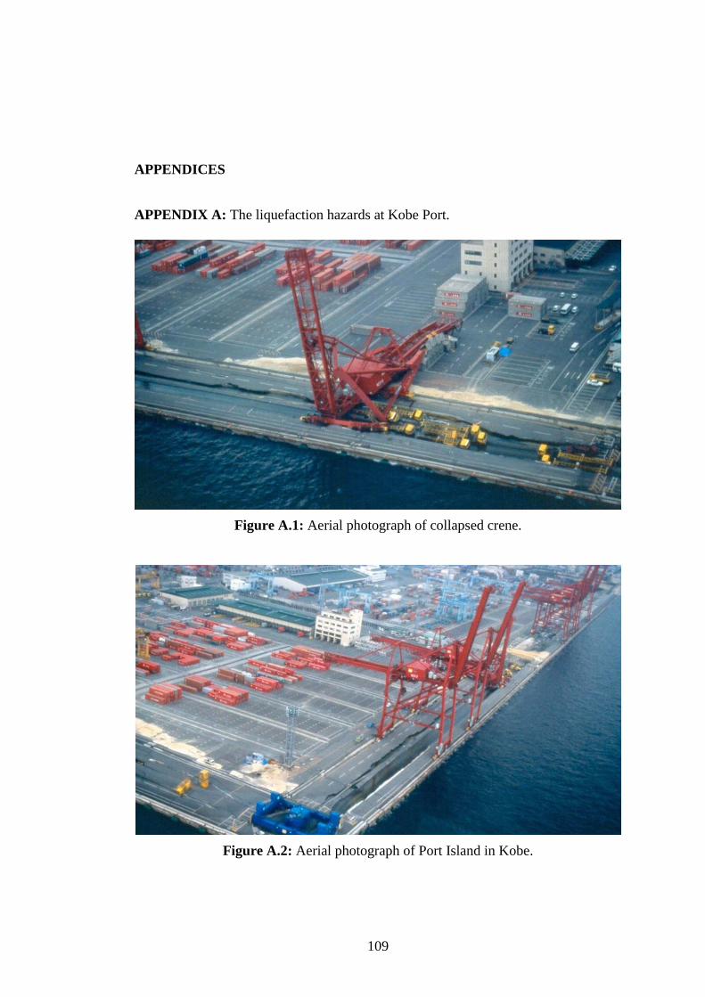
109
APPENDICES
APPENDIX A: The liquefaction hazards at Kobe Port.
Figure A.1: Aerial photograph of collapsed crene.
Figure A.2: Aerial photograph of Port Island in Kobe.
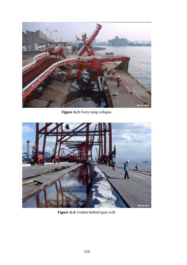
110
Figure A.3: Ferry ramp collapse.
Figure A.4: Graben behind quay wall.
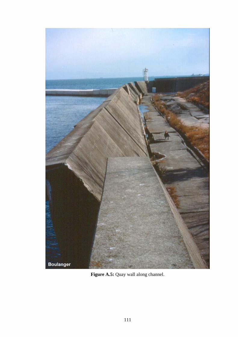
111
Figure A.5: Quay wall along channel.
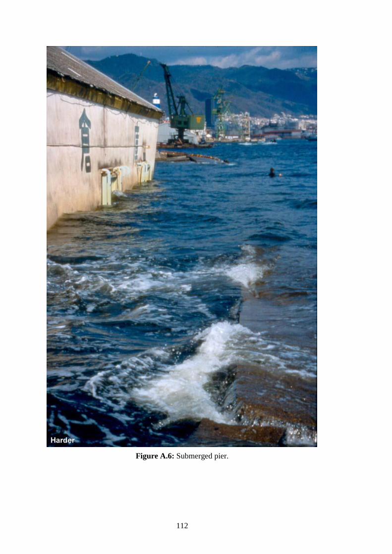
112
Figure A.6: Submerged pier.

113
APPENDIX B: Views and maps.
Figure B.1: Satellite View of Port Island, Kobe Port.
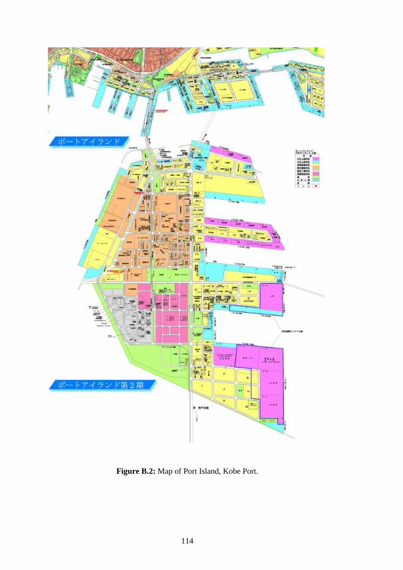
114
Figure B.2: Map of Port Island, Kobe Port.
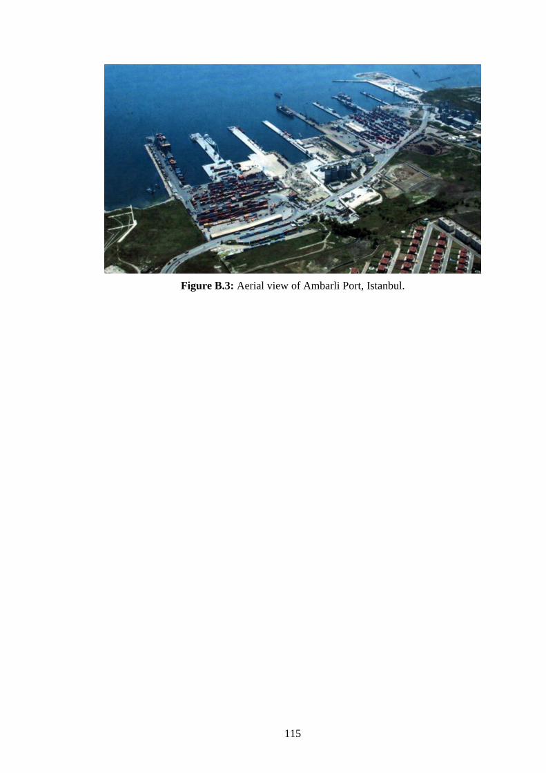
115
Figure B.3: Aerial view of Ambarli Port, Istanbul.

116

117
CURRICULUM VITAE
Name Surname : Hasan Giray BAKSI
Place and Date of Birth : ISTANBUL / 11.12.1982
E-Mail : [email protected]
EDUCATION :
2001: Haydarpaşa Lisesi (High School)
2008: Istanbul Technical University / Civil Engineering Program (Licence)
COMPUTER SKILLS :
SAP2000: Integrated Structural Analysis and Design, CSI, USA.
ETABS: Integrated Analysis, Design and Drafting of Building Systems,
CSI, USA.
SAFE: Slab Analysis using Finite Elements, CSI, USA.
PERFORM 3D: Nonlinear Analysis and Performance Assessment of 3-D
Structures, CSI America, USA.
AutoCAD: Computer-Aided Design Software, Autodesk, USA.
IdeCAD: Structural Analysis Software, IdeYapı, Turkey.
FIONA 3D: A General Purpose Object – Oriented Nonlinear FiniteElement
Program in C++”, North Carolina State University, Raleigh, NC, USA.
LANGUAGE :
English: Upper Intermediate.
Italian: Elementary.
118
PROFESSIONAL EXPERIENCE:
2009: BUYAKA Shopping Mall and Towers (Reinforced Concrete). Static
Project Drawing, Ümraniye, Istanbul, Turkey.
2010: Piri Reis University Campus (Reinforced Concrete). Static Project,
Modelling, Computing and Design, Tuzla, İstanbul, Turkey.
2011: Lasagrada Hotel (Reinforced Concrete), Retrofitting Static Project,
Modelling, Computing and Design, Şişli, İstanbul, Turkey.
2012: ETİ Management Center (Reinforced Concrete). Static Project
Modelling, Computing and Design, Eskişehir, Turkey.
2013: Dumankaya Ritim 44-Story Towers (Reinforced Concrete).
Modelling and Computing of Nonlinear Time History Analysis, Maltepe,
Istanbul, Turkey.
2014: Eren Holding Factory Building (Steel and Reinforced Concrete),
Modelling, Computing and Design, Eskişehir, Turkey.
2014: Park34 Residences and Penthouses Tower (Reinforced Concrete),
Static Project, Modelling, Computing and Design, Pendik, İstanbul, Turkey.
2015: Batı-Göz, Hospital (Reinforced Concrete). Retrofitting Project,
Üsküdar, İstanbul, Turkey.
2015: Cavit Paşa Kiosk (Timber). Restitution, Üsküdar, İstanbul.
2016: 3-Story Underground Car Park (Reinforced Concrete). Modelling,
Computing and Design, Kütahya, Turkey.
2016: Celalettin Bey Kiosk (Timber). Restitution, Üsküdar, İstanbul.
2016: Eryaman Stadium (Steel and Reinforced Concrete). Modelling,
Computing and Design, Ankara, Turkey.
2016: Sıraevler Project (Masonry). Retrofitting Project. Şişli, İstanbul,
Turkey.
2017: Model School. Vehbi KOC Foundation (Reinforced Concrete). Static
Project, Beykoz, İstanbul, Turkey.
2017: Büyükyalı Shopping Mall and Residences (Timber, Masonry, Steel
and Reinforced Concrete). Retrofitting Historical Buildings, Static Project and
Computing of Nonlinear Time History Analysis. Zeytinburnu, İstanbul, Turkey.
PUBLICATIONS, PRESENTATIONS AND PATENTS ON THE THESIS:
Baksı H. G. and Ülker M. B. C. (2017), “Analysis of Dynamic Response of a
Caisson Type Gravity Quay Wall – Seabed Soil System” Proc 27th International
Society Offshore and Polar Engineering Conference, San Francisco, USA ISOPE
(accepted).