Ivona Cetinić, Charles R. McClain, and P. Jeremy Werdell

NASA/TM–2018-219027/ Vol. 5

December 2018

National Aeronautics and Space Administration

Goddard Space Flight Center Greenbelt, Maryland 20771

PACE Technical Report Series, Volume 5Ivona Cetinić, Charles R. McClain, and P. Jeremy Werdell, Editors

Mission Formulation Studies

Paula Bontempi, Brian Cairns, Susanne E. Craig, André Dress, Bryan Franz, Robert Lossing, Antonio Mannino, Lachlan I. W. McKinna, Nima Pahlevan, Frederick S. Patt, Robert Schweiss, and Jeremy Werdell

Since its founding, NASA has been dedicated to the advancement of aeronautics and space science. The NASA scientific and technical information (STI) pro-gram plays a key part in helping NASA maintain this important role.

The NASA STI program operates under the auspices of the Agency Chief Information Officer. It collects, organizes, provides for archiving, and disseminates NASA’s STI. The NASA STI program provides access to the NASA Aeronautics and Space Database and its public interface, the NASA Technical Report Server, thus providing one of the largest collections of aero-nautical and space science STI in the world. Results are published in both non-NASA channels and by NASA in the NASA STI Report Series, which includes the following report types:

• TECHNICAL PUBLICATION. Reports of completed research or a major significant phase of research that present the results of NASA Programs and include extensive data or theoretical analysis. Includes compilations of significant scientific and technical data and information deemed to be of continuing reference value. NASA counterpart of peer-reviewed formal professional papers but has less stringent limitations on manuscript length and extent of graphic presentations.

• TECHNICAL MEMORANDUM. Scientific and technical findings that are preliminary or of specialized interest, e.g., quick release reports, working papers, and bibliographies that contain minimal annotation. Does not contain extensive analysis.

• CONTRACTOR REPORT. Scientific and technical findings by NASA-sponsored contractors and grantees.

• CONFERENCE PUBLICATION. Collected papers from scientific and technical conferences, symposia, seminars, or other meetings sponsored or co-sponsored by NASA.

• SPECIAL PUBLICATION. Scientific, technical, or historical information from NASA programs, projects, and missions, often concerned with subjects having substantial public interest.

• TECHNICAL TRANSLATION. English-language translations of foreign scientific and technical material pertinent to NASA’s mission.

Specialized services also include organizing and publishing research results, distributing specialized research announcements and feeds, providing help desk and personal search support, and enabling data exchange services. For more information about the NASA STI program, see the following:

• Access the NASA STI program home page at http://www.sti.nasa.gov

• E-mail your question via the Internet to [email protected]

• Phone the NASA STI Information Desk at 757-864-9658

• Write to: NASA STI Information Desk Mail Stop 148 NASA’s Langley Research CenterHampton, VA 23681-2199

NASA STI Program ... in Profile

NASA/TM–2018-219027/ Vol. 5

December 2018

PACE Technical Report Series, Volume 5Editors:Ivona Cetinić GESTAR/Universities Space Research Association, Columbia, Maryland Charles R. McClain Science Applications International Corporation, Reston, VirginiaP. Jeremy WerdellNASA Goddard Space Flight Center, Greenbelt, Maryland

Mission Formulation StudiesPaula Bontempi NASA Headquarters, Washington, DCBrian Cairns NASA Goddard Institute for Space Studies, New York, NYSusanne E. Craig GESTAR/Universities Space Research Association, Columbia, MDAndré Dress NASA Goddard Space Flight Center, Greenbelt, MDBryan Franz NASA Goddard Space Flight Center, Greenbelt, MDRobert Lossing Science Applications International Corporation, Reston, VA Antonio Mannino NASA Goddard Space Flight Center, Greenbelt, MD Lachlan I. W. McKinna Go2Q Pty Ltd, Buderim, AustraliaNima Pahlevan Science Systems and Applications Inc, Lanham, MD Frederick S. Patt Science Applications International Corporation, Reston, VARobert Schweiss NASA Goddard Space Flight Center, Greenbelt, MDJeremy Werdell NASA Goddard Space Flight Center, Greenbelt, MD

National Aeronautics and Space Administration

Goddard Space Flight Center Greenbelt, Maryland 20771

Notice for Copyrighted Information

This manuscript has been authored by employees of GESTAR/Universities Space Research Association, and Science Applications International Corporation, and Go2Q Pty Ltd (Buderim, Australia) with the National Oceanic and Atmospheric Administration and the National Aeronautics and Space Administration. The United States Government has a nonexclusive, irrevocable, worldwide license to prepare derivative works, publish or reproduce this manuscript for publication acknowledges that the United States Government retains such a license in any published form of this manuscript. All other rights are retained by the copyright owner.

NASA STI ProgramMail Stop 148 NASA’s Langley Research CenterHampton, VA 23681-2199

National Technical Information Service5285 Port Royal RoadSpringfield, VA 22161703-605-6000

Level of Review: This material has been technically reviewed by technical management.

Trade names and trademarks are used in this report for identification only. Their usage does not constitute an official endorsement, either expressed or implied, by the National Aeronautics and Space Administration.

Available from

Available in electronic form at http://

i

INTRODUCTION Introduction to Volume 5: Mission Formulation Studies

The Plankton, Aerosol, Cloud, ocean Ecosystem (PACE; https://pace.gsfc.nasa.gov) mission represents

NASA’s next great investment in satellite ocean color and the combined study of Earth’s ocean-

atmosphere system. At its core, PACE builds upon NASA’s multi-decadal legacies of the Coastal Zone

Color Scanner (1978-1986), Sea-viewing Wide Field-of-view Sensor (SeaWiFS; 1997-2010), Moderate

Resolution Imaging Spectroradiometers (MODIS) onboard Terra (1999-present) and Aqua (2002-

present), and Visible Infrared Imaging Spectroradiometer (VIIRS) onboard Suomi NPP (2012-present)

and JPSS-1 (2017-present; to be renamed NOAA-20). The ongoing, combined climate data record from

these instruments changed the way we view our planet and – to this day – offers an unparalleled

opportunity to expand our senses into space, compress time, and measure life itself.

This volume presents PACE Project scientific studies related to the general formulation of the mission

and PACE observatory – that is, those studies that influenced preliminary mission design during its Pre-

phase A (2014-2016; pre-formulation: define a viable and affordable concept) and Phase A (2016-2017;

concept and technology development). The volume begins with a history of the direction of the mission to

NASA Goddard Space Flight Center, then proceeds with topical summaries of various aspects of the

ocean color instrument (OCI) concept design and general observatory behavior (e.g., the need to tilt OCI

to mitigate contamination by Sun glint and the altitude at which it should be flown). Many of these

studies were integral in shaping an amorphous observatory concept into something viable and

scientifically meaningful. Subsequent volumes will capture more specific details related to fine-tuning of

the mission and the design of OCI.

I would like to congratulate the full PACE Project for maintaining the required bandwidth and enthusiasm

to whittle broad mission ideas and expectations into a viable mission concept, particularly under the

relentless reminders of being cost-capped. I would also like to thank the Project Science team for their

pursuit of these studies – and their subsequent documentation in this Technical Report series – that share

our experiences and lessons learned. We hope the user community enjoys and benefits from our sharing

of this journey.

P. J. Werdell

PACE Project Scientist

March 2018

ii

Contents

PACE Mission Formulation and Architecture ........................................................................................... 1

Executive Summary .................................................................................................................................. 1

Scientific Background ................................................................................................................. 1

Realizing the PACE Mission ....................................................................................................... 3

Mission Organization and Management ...................................................................................... 4

Mission Infrastructure.................................................................................................................. 5

Instrument Management and Organization ................................................................................. 9

Integration and Testing and Mission Operations ....................................................................... 10

Concluding Remarks ................................................................................................................. 11

Analysis of PACE OCI Coverage Loss from Glint and Tilt Change ....................................................... 12

Executive Summary ................................................................................................................................ 12

Introduction ............................................................................................................................... 12

Analysis Methods ...................................................................................................................... 13

2.2.1. PACE Geolocation Simulation .................................................................................................. 13

2.2.2. Tilt Change Strategy .................................................................................................................. 14

2.2.3. Sun Glint Simulation ................................................................................................................. 15

2.2.4. Global Coverage Analysis ......................................................................................................... 15

Results ....................................................................................................................................... 16

Conclusion ................................................................................................................................. 19

Case Study on the Science Data Completeness Requirement for PACE ................................................. 20


Introduction ............................................................................................................................... 20

Analysis ..................................................................................................................................... 20

3.2.1. A Review of Global Ocean Color Retrievals ............................................................................ 20

3.2.2. Analysis of Data Completeness ................................................................................................. 21

Discussion and Conclusion ........................................................................................................ 24

Appendix A. .............................................................................................................................. 26

Assessment of Hyperspectral Pushbroom Image Striping Artifacts in Ocean Color Products............... 28


Introduction ............................................................................................................................... 28

Heritage Instrument Data........................................................................................................... 29

Pushbroom Conceptual Model .................................................................................................. 32

iii

Example of Synthesized Pushbroom Striping ........................................................................... 34

Impact of Striping on Derived Products .................................................................................... 35

Impact of Striping on Deriviative Spectroscopy ....................................................................... 36

Case Study of Destriping Method ............................................................................................. 37

Summary and Conclusion .......................................................................................................... 39

Analysis of Potential PACE Altitude Reduction ....................................................................................... 43


Introduction ............................................................................................................................... 43

Considerations for Altitude Reduction ...................................................................................... 43

5.2.1. Mission Science ......................................................................................................................... 43

5.2.2. Global Coverage ........................................................................................................................ 44

5.2.3. Orbit Maintenance ..................................................................................................................... 48

5.2.4. OCI Impacts ............................................................................................................................... 48

5.2.5. Spacecraft Impacts ..................................................................................................................... 49

Conclusion ................................................................................................................................. 50

PACE OCI Proxy Data Development ........................................................................................................ 51


Introduction ............................................................................................................................... 51

PACE OCI Assumed Spectral Channels ................................................................................... 51

PACE OCI Assumed Level-1B Format ..................................................................................... 51

PACE OCI Proxy Data Derived from AVIRIS Classic (OCIA) ............................................... 52

PACE Instrument Design Lab Studies – Summary and Overview on Meeting Science Requirements . 56

Introduction ............................................................................................................................... 56

OCI Study Parameters and Requirements ................................................................................. 59

Multi-Angle Polarimeter............................................................................................................ 63

Coastal Camera .......................................................................................................................... 64

Appendix A: PACE Program Science Trades and Feasibility Study Document ...................... 66

7.5.1. Trade Studies on PACE. ............................................................................................................ 66

Appendix B: Coastal Camera Request for Information (RFI) ................................................... 70

Case for the Addition of a Coastal Ocean Color Imager (COCI) to PACE ............................................. 74


Introduction ............................................................................................................................... 74

Science Justification .................................................................................................................. 75

8.2.1. Ocean Color Measurements ....................................................................................................... 76

8.2.2. Atmospheric Measurements ...................................................................................................... 77

iv

Science Questions Addressed by COCI .................................................................................... 78

COCI Applied Science Objectives: ........................................................................................... 79

Summary .................................................................................................................................... 79

Appendix A ............................................................................................................................... 84

Appendix B. PACE Mission Applications White Papers pertaining to COCI .......................... 85

Analysis of a Pushbroom Ocean Color Instrument Lunar Calibration ................................................... 86


Introduction ............................................................................................................................... 86

9.1.1. Inputs ......................................................................................................................................... 87

9.1.2. Maneuver Sequence ................................................................................................................... 87

Analysis ..................................................................................................................................... 88

9.2.1. Timing ....................................................................................................................................... 88

9.2.2. Maneuver Accuracy and Stability ............................................................................................. 89

9.2.3. Geometry and Viewing .............................................................................................................. 89

9.2.4. Lunar Disk Sampling Analysis .................................................................................................. 90

Mission Impacts ......................................................................................................................... 91

Summary of Key Requirements ................................................................................................ 91

References .................................................................................................................................................. 92

1

Chapter 1

PACE Mission Formulation and Architecture

Jeremy Werdell, NASA Goddard Space Flight Center, Greenbelt, Maryland1

Paula Bontempi, NASA Headquarters, Washington, DC

Andre’ Dress, NASA Goddard Space Flight Center, Greenbelt, Maryland

Bryan Franz, NASA Goddard Space Flight Center, Greenbelt, Maryland

Robert Schweiss, NASA Goddard Space Flight Center, Greenbelt, Maryland

1.

Executive Summary

This chapter summarizes the mission architecture for the Plankton, Aerosol, Cloud, ocean Ecosystem

(PACE) mission, ranging from its scientific rationale to the history of its realized conception to its

present-day organization and management. This volume in the PACE Technical Report series focuses on

trade studies that informed the formulation of the mission in its pre-Phase A (2014-2016; pre-formulation:

define a viable and affordable concept) and Phase A (2016-2017; concept and technology development).

With that in mind, this chapter serves to introduce the mission by providing: (1) a brief summary of the

science drivers for the mission; (2) a history of the direction of the mission to NASA’s Goddard Space

Flight Center (GSFC); (3) a synopsis of the mission’s and instruments’ management and development

structures; and (4) a brief description of the primary components and elements that form the foundation of

the mission, encompassing the major mission segments (space, ground, and science data processing) and

their roles in integration, testing, and operations.

Scientific Background

Global ocean color measurements are essential for understanding ocean ecology and the global carbon

cycle and how it affects and is affected by climate change. A key step toward helping scientists

understand how the Earth has responded to its changing climate over time – and how it may respond in

the future – is through the establishment of high-quality, long-term, global time series of various

geophysical parameters. Given the nature of the phenomena and the timescales needed to distinguish

trends, such measurements will require combining data from several missions. These climate-quality time

series are called climate data records (CDRs), and are being generated for a variety of geophysical

parameters, including ocean color. Additionally, the mission seeks to move beyond heritage sensor

capabilities and data products to allow measurements of new biogeochemical properties, such as

phytoplankton community contribution (that is, the discrimination of different classes of phytoplankton

and their global distributions).

Dissolved and suspended organic and inorganic material within the upper layer of ocean water

provide the basis for ocean color science. Many particulate and dissolved constituents of the near-surface

water column absorb and scatter light differently in the ultraviolet (UV) and visible (VIS) regions of the

electromagnetic spectrum (these are the colors that humans see). At its most fundamental level, ocean

1 Cite as: Werdell, P. J., P. Bontempi, A. Dress, B. Franz, and R. Schweiss (2018), PACE Mission Formulation and Architecture,

in PACE Technical Report Series, Volume 5: Mission Formulation Studies (NASA/TM-2018 – 2018-219027/ Vol. 5), edited by

I. Cetinić, C. R. McClain and P. J. Werdell, NASA Goddard Space Flight Space Center Greenbelt, MD.

2

color science is about relating the spectral variations in the UV-VIS marine light field (that is, differences

in the ocean’s color) to the concentrations of the various constituents residing in the sunlit, near-surface

water column.

The requirements for PACE’s primary instrument, the Ocean Color Instrument (OCI), predominantly

focus on improving our ability to observe phytoplankton. These microscopic algae form the base of the

marine food chain and produce some of the oxygen we breathe. They also play an important role in

converting inorganic carbon in carbon dioxide (CO2) to organic compounds, fueling global ocean

ecosystems and driving oceanic biogeochemical cycles through grazing (i.e., they provide a food source

for zooplankton) and their degradation products via the microbial loop (where bacteria reintroduce

dissolved organic carbon and nutrients to the water, effectively recycling both back into the food web).

Phytoplankton are therefore a critical part of the ocean’s biological carbon pump, whereby atmospheric

CO2 gets sequestered to the deep ocean, and are responsible for roughly half of Earth’s net primary

production. Phytoplankton growth, however, is highly sensitive to variations in ocean and atmospheric

physical properties, such as upper-ocean stratification, nutrient concentrations (e.g., nitrate and iron) and

light availability within this mixed layer. They also vary greatly in their size, function, response to

ecosystem changes or stresses, and nutritional value for species higher in the food web. Hence,

measurements of phytoplankton community composition and their distributions remain essential for

understanding global carbon cycles and how living marine resources are responding to Earth’s changing

climate.

While PACE is predominantly an ocean color mission, it will also have secondary objectives and two

secondary instruments, both multi-angle polarimeters. An additional overarching goal for the mission is to

help determine the roles of the ocean and atmosphere in global biogeochemical cycling and how

perturbations to Earth’s energy balance both affect and are affected by rising atmospheric CO2 levels and

Earth’s changing climate. The PACE mission will contribute to the continuation of atmospheric CDRs as

well as those for ocean color. The OCI will allow continuation of heritage aerosol measurements made

using MODIS onboard Terra and Aqua and the Ozone Monitoring Instrument (OMI) onboard Aura. It

will also provide additional characterization of aerosol particles because its spectral range will include

shortwave infrared wavelengths. This will enable continuation of MODIS-like and OMI-like

characterization of aerosol properties, MODIS-like measurements of water vapor, and MODIS-like

retrievals of some cloud optical properties. These are the key atmospheric components affecting our

ability to predict climate change as they contribute the largest uncertainties in our understanding of

climate forcings and cloud feedbacks in an increasingly warmer planet. The interactions between these

species are key to such understanding, as aerosols, water vapor, and clouds remain intertwined within the

hydrologic cycle because most cloud droplets are seeded by small aerosol particles called cloud

condensation nuclei. Changes in the amount, type, and distribution of aerosols, therefore, can alter the

micro- and macro-physical characteristics of clouds. Furthermore, natural and anthropogenic changes to

the aerosol system may affect clouds and precipitation, which can alter where, when, and how much

precipitation may fall.

A summary of PACE science objectives are as follows:

• Extending key systematic ocean biological, ecological, and biogeochemical data records and

cloud and aerosol data records;

• Making global measurements of ocean color data products that are essential for understanding the

global carbon cycle and ocean ecosystem responses to a changing climate, as well as managing

marine fisheries and water quality;

3

• Collecting global observations of aerosol and cloud properties, focusing on reducing the largest

uncertainties in climate and radiative forcing models of the Earth system; and,

• Improving our understanding of how aerosols influence ocean ecosystems and biogeochemical

cycles and how ocean biological and photochemical processes affect the atmosphere, as well as

understanding air quality.

Volumes 1 and 2 of this Technical Memorandum series (ACE Ocean Working Group

recommendations and instrument requirements for an advanced ocean ecology mission [2018] and The

PACE Science Definition Team Report [2018]) expand on the rationale for PACE.

Realizing the PACE Mission

The PACE mission is a strategic climate continuity mission that was formally first defined in the 2010

document Responding to the Challenge of Climate and Environmental Change: NASA’s Plan for Climate-

Centric Architecture for Earth Observations and Applications from Space

(http://science.nasa.gov/media/medialibrary/2010/07/01/Climate_Architecture_Final.pdf). This Climate

Initiative complements NASA’s implementation of the National Research Council’s 2007 Decadal

Survey of Earth Science at NASA, the National Oceanic and Atmospheric Administration (NOAA), and

the United States Geological Survey (USGS), entitled Earth Science and Applications from Space:

National Imperatives for the Next Decade and Beyond. From 2011-2012, NASA HQ convened a PACE

Science Definition Team, whose report provides overall scientific guidance for the mission during its

formulation and execution (see [PACE Science Definition Team, 2018]).

NASA HQ directed the PACE mission to GSFC in January 2014. The scope of this direction included

overall mission management (e.g., budget and schedule), safety and mission assurance, acquisition of the

spacecraft and launch vehicle, integration and testing of all mission elements, mission operations and

ground systems, development of the ocean color instrument (OCI), day-to-day scientific guidance related

to mission formulation and execution, and science data processing. NASA HQ specifically assigned

science data processing to the GSFC Ocean Biology Processing Group (OBPG;

https://oceancolor.gsfc.nasa.gov). NASA HQ allocated a not-to-be-exceeded $805M to the mission –

$705M to be managed by GSFC and $100M to be managed independently by HQ’s Earth Science

Division (ESD). The GSFC $705M encompasses all elements listed above with the exception of science

data processing. The ESD $100M encompasses science data processing, calibration and validation

systems (including a vicarious calibration instrument system), and all competed community science

teams. NASA HQ also directed GSFC to explore acquisition of a polarimeter as an optional secondary

instrument within their $705M allocation, to be obtained from the NASA Jet Propulsion Laboratory

(JPL), procured commercially, or contributed by entity external to GSFC.

In addition, NASA HQ directed mission development to be guided by a Design-to-Cost (DTC)

process. Within DTC, all elements of the mission other than the cost are in a tradeable space guided by

mission studies that are performed across all mission elements. In practice, mission studies result in

definition of approaches within and across elements that maximize science capabilities at a high cost

confidence. Volumes 3 (this volume) through 5 of this Technical Report series document scientific

mission studies that guided mission formulation.

4

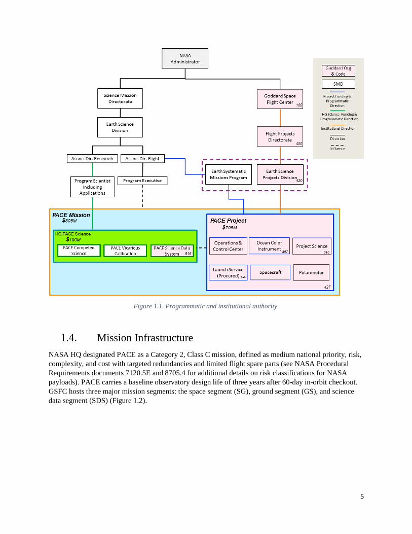
Mission Organization and Management

Project implementation authority is delegated from the NASA Associate Administrator for the Science

Mission Directorate to ESD, with mission execution directed to GSFC (Figure 1.1). The GSFC directed

work falls under the Earth Systematic Missions Program, which is administratively located within the

Flight Projects Directorate at GSFC. The PACE Project (Figure 1.1; lower right pink box; $705M) and

HQ Program Science (Figure 1.1; lower left green box; $100M) work collaboratively through the life of

the mission to ensure its scientific value and ultimate mission success. Briefly, Project responsibilities at

GSFC include design, development, manufacturing, integration and test, verification, documentation, and

mission operations. Key roles not described elsewhere in this chapter include:

• A Project Manager that is responsible and accountable for technical, cost, schedule management,

and performance;

• A Project Scientist that is responsible for the ongoing scientific output through all phases of the

mission (data and, by extension, sensor characteristics and performance, as well as ongoing

instrument calibration and science product validation);

• A Mission System Engineer that provides ultimate engineering technical authority for all mission

systems and elements; and,

• A Chief Safety and Mission Assurance Officer that provides independent technical authority for

all flight assurance and safety disciplines of the Project.

Briefly, HQ Program Science responsibilities include establishment of competed science teams, provision

of the vicarious calibration and validation system(s), and supporting the science data segment (SDS)

located within the OBPG. Key roles within PACE include:

• A Program Scientist that is responsible for ensuring maximization of science output of the

mission, in particular verifying that important areas of science are not neglected; and,

• A Program Executive that is responsible for ensuring the Project successfully passes all HQ gate

reviews, obtaining HQ concurrence on Project plans, and development of Project budget

guidelines.

5

Figure 1.1. Programmatic and institutional authority.

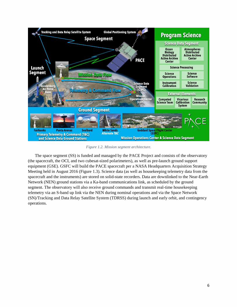
Mission Infrastructure

NASA HQ designated PACE as a Category 2, Class C mission, defined as medium national priority, risk,

complexity, and cost with targeted redundancies and limited flight spare parts (see NASA Procedural

Requirements documents 7120.5E and 8705.4 for additional details on risk classifications for NASA

payloads). PACE carries a baseline observatory design life of three years after 60-day in-orbit checkout.

GSFC hosts three major mission segments: the space segment (SG), ground segment (GS), and science

data segment (SDS) (Figure 1.2).

6

Figure 1.2. Mission segment architecture.

The space segment (SS) is funded and managed by the PACE Project and consists of the observatory

(the spacecraft, the OCI, and two cubesat-sized polarimeters), as well as pre-launch ground support

equipment (GSE). GSFC will build the PACE spacecraft per a NASA Headquarters Acquisition Strategy

Meeting held in August 2016 (Figure 1.3). Science data (as well as housekeeping telemetry data from the

spacecraft and the instruments) are stored on solid-state recorders. Data are downlinked to the Near-Earth

Network (NEN) ground stations via a Ka-band communications link, as scheduled by the ground

segment. The observatory will also receive ground commands and transmit real-time housekeeping

telemetry via an S-band up link via the NEN during nominal operations and via the Space Network

(SN)/Tracking and Data Relay Satellite System (TDRSS) during launch and early orbit, and contingency

operations.

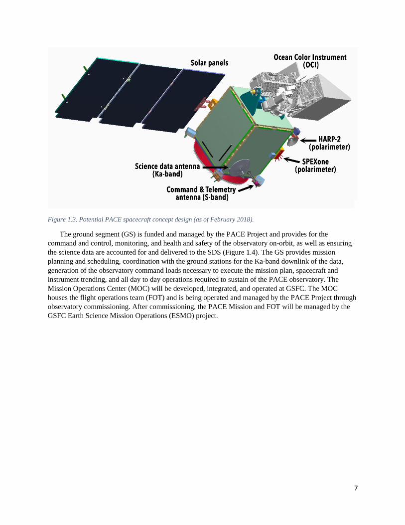
7

Figure 1.3. Potential PACE spacecraft concept design (as of February 2018).

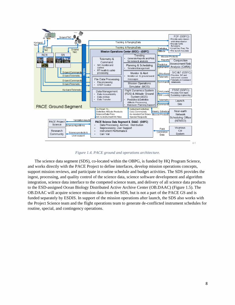
The ground segment (GS) is funded and managed by the PACE Project and provides for the

command and control, monitoring, and health and safety of the observatory on-orbit, as well as ensuring

the science data are accounted for and delivered to the SDS (Figure 1.4). The GS provides mission

planning and scheduling, coordination with the ground stations for the Ka-band downlink of the data,

generation of the observatory command loads necessary to execute the mission plan, spacecraft and

instrument trending, and all day to day operations required to sustain of the PACE observatory. The

Mission Operations Center (MOC) will be developed, integrated, and operated at GSFC. The MOC

houses the flight operations team (FOT) and is being operated and managed by the PACE Project through

observatory commissioning. After commissioning, the PACE Mission and FOT will be managed by the

GSFC Earth Science Mission Operations (ESMO) project.

8

Figure 1.4. PACE ground and operations architecture.

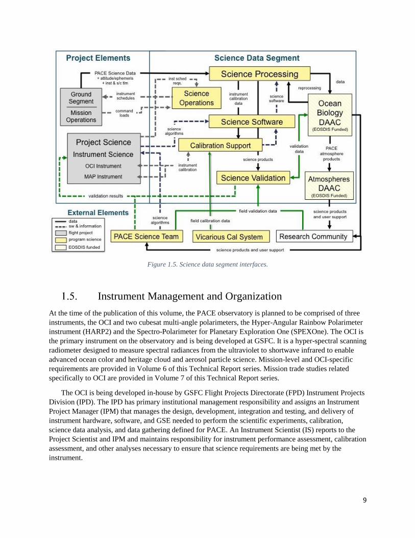
The science data segment (SDS), co-located within the OBPG, is funded by HQ Program Science,

and works directly with the PACE Project to define interfaces, develop mission operations concepts,

support mission reviews, and participate in routine schedule and budget activities. The SDS provides the

ingest, processing, and quality control of the science data, science software development and algorithm

integration, science data interface to the competed science team, and delivery of all science data products

to the ESD-assigned Ocean Biology Distributed Active Archive Center (OB.DAAC) (Figure 1.5). The

OB.DAAC will acquire science mission data from the SDS, but is not a part of the PACE GS and is

funded separately by ESDIS. In support of the mission operations after launch, the SDS also works with

the Project Science team and the flight operations team to generate de-conflicted instrument schedules for

routine, special, and contingency operations.

9

Figure 1.5. Science data segment interfaces.

Instrument Management and Organization

At the time of the publication of this volume, the PACE observatory is planned to be comprised of three

instruments, the OCI and two cubesat multi-angle polarimeters, the Hyper-Angular Rainbow Polarimeter

instrument (HARP2) and the Spectro-Polarimeter for Planetary Exploration One (SPEXOne). The OCI is

the primary instrument on the observatory and is being developed at GSFC. It is a hyper-spectral scanning

radiometer designed to measure spectral radiances from the ultraviolet to shortwave infrared to enable

advanced ocean color and heritage cloud and aerosol particle science. Mission-level and OCI-specific

requirements are provided in Volume 6 of this Technical Report series. Mission trade studies related

specifically to OCI are provided in Volume 7 of this Technical Report series.

The OCI is being developed in-house by GSFC Flight Projects Directorate (FPD) Instrument Projects

Division (IPD). The IPD has primary institutional management responsibility and assigns an Instrument

Project Manager (IPM) that manages the design, development, integration and testing, and delivery of

instrument hardware, software, and GSE needed to perform the scientific experiments, calibration,

science data analysis, and data gathering defined for PACE. An Instrument Scientist (IS) reports to the

Project Scientist and IPM and maintains responsibility for instrument performance assessment, calibration

assessment, and other analyses necessary to ensure that science requirements are being met by the

instrument.

10

Both the HARP2 and SPEXOne are acquired outside of GSFC and will be described in detail in a

subsequent volume in this series. The HARP2 is a contribution to PACE by the University of Maryland

Baltimore County (UMBC) and the SPEXOne is a contribution to PACE from the Netherlands Institute

for Space Research (SRON). These instruments will be developed and qualified at the developer’s home

institution. Following a successful Pre-ship Review, where requirements will be verified by the Project,

each instrument will be formally delivered to the PACE Project. The instruments will be integrated on to

the spacecraft at the GSFC. Project Science will work with the instrument providers through the life of the

mission.

Integration and Testing and Mission Operations

The Integration and Testing (I&T) effort will be managed by the PACE Project and executed by the I&T

team, spacecraft subsystem teams, instrument teams, and ground system teams at GSFC. This effort will

demonstrate that the flight hardware and ground system hardware comply with the mission requirements.

All components will be fully qualified, including environmental testing, prior to delivery to I&T. The

OCI Team is responsible for the integration, performance testing, and environmental testing of the OCI at

GSFC. The Polarimeter providers are responsible for the integration, performance testing, and

environmental testing of the polarimeter instruments at the provider facilities. Upon completion, the

instruments will be delivered to the spacecraft at GSFC for spacecraft integration and testing. Prior to the

instrument integration onto the spacecraft, interface simulators will be used to verify the interfaces and

software.

Once the PACE observatory is fully integrated and configured, observatory testing will be performed

including comprehensive performance tests. Observatory tests will include environmental tests that are

appropriate at the observatory level including thermal vacuum, vibration, acoustics, electromagnetic

interference/compatibility, and magnetics. Observatory testing will also include mission simulations and

end-to-end testing with the ground system to ensure command and telemetry capability with the mission

and science control centers. These mission simulation exercises will also validate nominal and

contingency mission operations procedures and provide operator training. Recorded and real-time satellite

data will be relayed through the operational ground system to verify data compatibility with the ground

system and data processing facility. At the completion of the observatory performance, environmental,

and mission test program, the Project will ship the observatory to the launch site. The observatory will be

processed at the payload processing facility and integrated onto the launch vehicle.

All PACE operations will be located at GSFC. The observatory flight operations will be conducted

from the GSFC MOC. The MOC will perform all real-time operations and off-line operations functions,

including planning and scheduling, orbit and attitude analysis, housekeeping telemetry data processing,

monitoring/managing the spacecraft and instruments, first line health/safety for the instruments, and

housekeeping archiving and analysis. In support of the mission operations, the SDS works with the

Project Science team and the flight operations team to generate de-conflicted instrument activity

schedules for routine, special, and contingency operations. This instrument activity schedule is provided

to the mission operations team, located at the MOC, for mission planning and integration with

observatory activities and ground contact schedules.

11

Concluding Remarks

The PACE mission represents NASA’s next great investment in satellite ocean color and the combined

study of Earth’s ocean-atmosphere system. This chapter serves as an introduction to this volume by

summarizing the mission architecture, ranging from its scientific rationale to the history of its realized

conception to its present-day organization and management. The remainder of this volume provides

topical summaries of various aspects of the OCI concept design and general observatory behavior. Many

of these studies were integral in shaping an amorphous observatory concept into something viable and

scientifically meaningful.

12

Chapter 2

Analysis of PACE OCI Coverage Loss from Glint and

Tilt Change

Frederick S. Patt, Science Applications International Corporation, Reston, Virginia2

2.

Executive Summary

The Phytoplankton, Aerosol, Cloud, ocean Ecosystem (PACE) Ocean Color Instrument (OCI) is required

to mitigate Sun glint from the ocean surface. This mitigation is performed by tilting the instrument field-

of-regard along-track, aft prior to the spacecraft subsolar point in the orbit and forward after this point. A

capability has been developed to model the combined effects of the glint and tilt change on global

coverage. This paper describes the methods and presents sample results. The results have been used to

arrive at a mission requirement to perform the tilt change in 60 seconds to limit the combined global

coverage loss from high glint and the tilt change.

Introduction

The Plankton, Aerosol, Cloud, ocean Ecosystem (PACE) mission is a polar-orbiting, Earth remote

sensing mission that is planned to launch in 2022. The primary instrument on the PACE observatory is

the Ocean Color Instrument (OCI). The OCI is a hyper-spectral scanning (HSS) radiometer designed to

measure radiances continuously in the ultraviolet to near-infrared spectral region over the range 350 to

800 nm, and in the near-infrared to short wave infrared (SWIR) spectral region. The OCI threshold spatial

resolution is approximately 1 km-squared at nadir with 2-day global coverage. The OCI design has a

scanning telescope with a field of regard of +/- 56.5 degrees across track. PACE will be launched into a

Sun-synchronous orbit at an altitude of 676.5 nm and an ascending node crossing local time of 13:00.

A significant contaminant of ocean remote-sensing data is sunlight reflected from the ocean surface,

known as Sun glint. The magnitude and extent of Sun glint is a function of viewing geometry, solar

illumination and wind speed [Cox and Munk, 1954]. The effects of glint can be modelled and corrected up

to a point, but severe (“high”) glint, which occurs close to the specular reflection geometry, degrades the

science data quality and therefore reduces effective coverage, i.e, it is “masked” and not used to derive

data products.

The most effective glint mitigation strategy is to rotate, or tilt, the sensor view along-track, thereby

shifting the sensor view away from specular reflection angles and reducing the glint magnitude. Tilting

can be performed by either the sensor or the spacecraft; in the latter case, the tilt is performed by a pitch

maneuver. Past sensors designed specifically for ocean color remote sensing, including the Coastal Zone

Color Scanner (CZCS), Ocean Color and Temperature Scanner (OCTS) and Sea-viewing Wide Field-of-

view Sensor (SeaWiFS), had a tilt capability included in the sensor design.

2 Cite as: Patt, F. S. (2018), Analysis of PACE OCI Coverage Loss from Glint and Tilt Change, in PACE Technical Report

Series, Volume 5: Mission Formulation Studies (NASA/TM-2018 – 2018-219027/ Vol. 5), edited by I. Cetinić, C. R. McClain and

P. J. Werdell, NASA Goddard Space Flight Space Center Greenbelt, MD.

13

The most commonly used tilt angle is 20 degrees. CZCS had a commandable range for the tilt angle

of the scanning mirror (not the entire instrument), and while in the beginning of the mission tilt angles

less than 20 degrees were used, soon after was decided to always command the tilt to 20 degrees. Both

OCTS (scan mirror) and SeaWiFS (spacecraft pitch) had commandable tilt angles of +/- 20 degrees and 0

(i.e., nadir).

In order to effectively reduce Sun glint, the sensor must be tilted away from the orbit subsolar point

(the point in the orbit where the subsatellite track is closest to the Earth subsolar location). This requires

that the tilt angle be changed from aft to forward at or near the subsolar point. The tilt change results in a

gap in sensor coverage, resulting from the combination of the change in viewing geometry and the time

required for the change. Although the sensor does not stop collecting data during the tilt change, the

pointing knowledge is less accurate, so the data are flagged. At the PACE altitude, the change in the tilt

angle results in a gap of about 4.5 degrees latitude, plus 0.061 seconds for each second of tilt change time

plus settling.

Although tilting the sensor is effective at reducing the glint, some amount of data will be lost to high

glint even at a tilt angle of 20 degrees. This, plus the tilt change coverage loss, results in a net loss of

coverage that depends on the tilt angle and change time. The method used to analyze the loss in coverage

and the results for a range of tilt angles and change times are presented in the following sections.

Analysis Methods

The PACE Level 1 requirement (when this chapter was written) is to achieve two-day coverage for OCI

within the solar zenith angle limit of 75 degrees. This analysis was structured to determine the impact of

high glint and the tilt change as they relate to data losses within this two-day coverage. The analysis

consisted of the following stages:

A. Simulate PACE geolocation for the mission orbit and OCI viewing geometry.

B. Develop a tilt change strategy to maximize two-day coverage for a given tilt angle and change

time.

C. Simulate the Sun glint based on the sensor geolocation.

D. Determine the loss in global coverage over a two-day period.

Each of these steps is described in the following sections.

2.2.1. PACE Geolocation Simulation

The simulation of PACE geolocation involves the following steps:

1. Simulate the PACE orbit

2. Construct the OCI view vectors

3. Compute the OCI geolocation for each desired time sample

To reduce the time required for the analysis runs, it was decided to subsample the PACE geolocation for

the simulation. Specifically, the scan period was set to 2 seconds and the scan angle interval to 0.5 degree,

compared to 1/6 second and 0.085 degree for OCI. These settings correspond to a maximum GSD of 18

km. As will be explained below, the coverage analysis used a spatial resolution coarser than this GSD, so

the subsampling had no effect on the results.

14

The PACE orbit was simulated for March 24 and 25, 2020. The simulation was performed using a set

of two-line elements (TLEs) and the SGP4 orbit model software. The TLEs were based on a set provided

by the Flight Dynamics Facility (FDF), representing the PACE orbit described in the Introduction, and

modified for an epoch of 00:00 UTC on March 24, 2020. The SGP4 model was run with a 1-minute

sample interval, and the output was then interpolated to 2-second intervals using the method of Patt

[2002]. Only the ascending orbit samples were used, corresponding to the daylit part of the orbit.

The OCI view vectors were based on a simple, planar scan model, representing the ideal sensor scan

geometry; in the sensor reference frame, the vectors lie in the Y-Z plane, where +Z is the scan center. The

vectors were constructed, as stated above, at 0.5-degree intervals over the scan angle range of +/-56.5

degrees, or 227 samples per scan.

The geolocation calculations were performed using the method of Patt and Gregg [1994]. The tilt

angle was set as the pitch angle for the sensor attitude (the roll and yaw were set to zero). The tilt change

strategy is described in the following section. The output of the geolocation includes the viewed location

(geodetic longitude and latitude) for each sample, sensor zenith and azimuth and solar zenith and azimuth;

the zenith and azimuth angles are used for the glint calculation and also for data selection during the

coverage analysis.

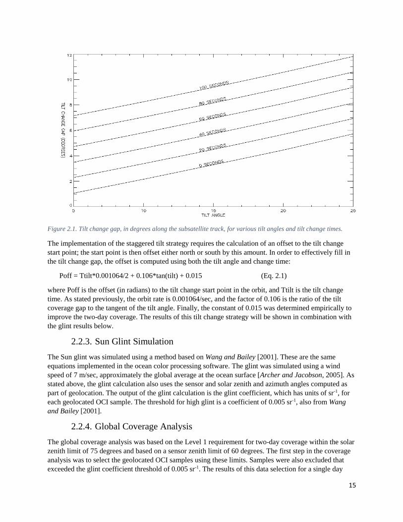
2.2.2. Tilt Change Strategy

The tilt change results in a gap in the science data; the size of the gap depends on the tilt angle and change

time. The size of the gap vs. tilt angle and change time is illustrated in Figure 2.1. If the tilt change is

always performed at the subsolar point each orbit, a persistent gap in global coverage around this latitude

range will result. Although the subsolar point moves north and south during the year, on shorter time

scales this gap would be present in global data.

For SeaWiFS, a strategy was developed to stagger the tilt change point in the orbit in order to fill in

the coverage gap [Gregg and Patt, 1994]. The strategy was to shift the tilt change latitude north of the

subsolar point for two consecutive days, and then south for the next two days. Thus, over a four-day

period the high glint and tilt change gaps were largely filled in.

For the OCI tilt analysis, a two-day tilt stagger strategy was developed. This was based on two

factors: 1) the period used for the analysis was two days, based on the Level 1 requirement; 2) the

difference between the PACE and SeaWiFS orbits results in a shift in the glint pattern off-center for OCI

and a difference in the day-to-day shift in the orbit tracks for PACE compared to SeaWiFS. It was

confirmed using the simulations that the two-day strategy resulted in better two-day coverage for the

PACE orbit.

As stated above, the subsolar point in the orbit is the point where the orbit track is closest to the

subsolar point on the Earth. For the PACE orbit (13:00 local time ascending node) this point will be

slightly north of the subsolar latitude. During actual OCI scheduling the subsolar point will be computed

each orbit using the actual orbit track and Sun vector; however, given the limited duration of this

simulation, the subsolar point was estimated to be 0.035 above the solar latitude (all angles in radians).

The nominal (non-staggered) tilt change start point was determined using the orbit rate (0.001064/sec)

and the tilt change time; the start point was shifted south by half of the tilt change time.

15

Figure 2.1. Tilt change gap, in degrees along the subsatellite track, for various tilt angles and tilt change times.

The implementation of the staggered tilt strategy requires the calculation of an offset to the tilt change

start point; the start point is then offset either north or south by this amount. In order to effectively fill in

the tilt change gap, the offset is computed using both the tilt angle and change time:

Poff = Ttilt*0.001064/2 + 0.106*tan(tilt) + 0.015 (Eq. 2.1)

where Poff is the offset (in radians) to the tilt change start point in the orbit, and Ttilt is the tilt change

time. As stated previously, the orbit rate is 0.001064/sec, and the factor of 0.106 is the ratio of the tilt

coverage gap to the tangent of the tilt angle. Finally, the constant of 0.015 was determined empirically to

improve the two-day coverage. The results of this tilt change strategy will be shown in combination with

the glint results below.

2.2.3. Sun Glint Simulation

The Sun glint was simulated using a method based on Wang and Bailey [2001]. These are the same

equations implemented in the ocean color processing software. The glint was simulated using a wind

speed of 7 m/sec, approximately the global average at the ocean surface [Archer and Jacobson, 2005]. As

stated above, the glint calculation also uses the sensor and solar zenith and azimuth angles computed as

part of geolocation. The output of the glint calculation is the glint coefficient, which has units of sr-1, for

each geolocated OCI sample. The threshold for high glint is a coefficient of 0.005 sr-1, also from Wang

and Bailey [2001].

2.2.4. Global Coverage Analysis

The global coverage analysis was based on the Level 1 requirement for two-day coverage within the solar

zenith limit of 75 degrees and based on a sensor zenith limit of 60 degrees. The first step in the coverage

analysis was to select the geolocated OCI samples using these limits. Samples were also excluded that

exceeded the glint coefficient threshold of 0.005 sr-1. The results of this data selection for a single day

16

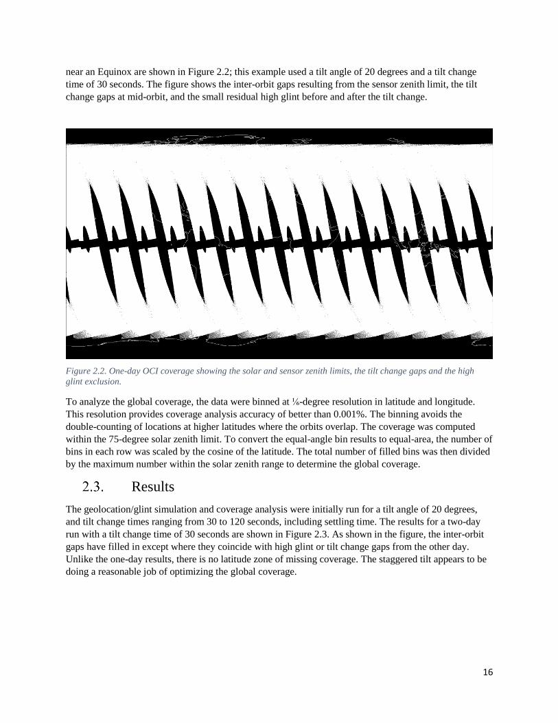
near an Equinox are shown in Figure 2.2; this example used a tilt angle of 20 degrees and a tilt change

time of 30 seconds. The figure shows the inter-orbit gaps resulting from the sensor zenith limit, the tilt

change gaps at mid-orbit, and the small residual high glint before and after the tilt change.

Figure 2.2. One-day OCI coverage showing the solar and sensor zenith limits, the tilt change gaps and the high

glint exclusion.

To analyze the global coverage, the data were binned at ⅙-degree resolution in latitude and longitude.

This resolution provides coverage analysis accuracy of better than 0.001%. The binning avoids the

double-counting of locations at higher latitudes where the orbits overlap. The coverage was computed

within the 75-degree solar zenith limit. To convert the equal-angle bin results to equal-area, the number of

bins in each row was scaled by the cosine of the latitude. The total number of filled bins was then divided

by the maximum number within the solar zenith range to determine the global coverage.

Results

The geolocation/glint simulation and coverage analysis were initially run for a tilt angle of 20 degrees,

and tilt change times ranging from 30 to 120 seconds, including settling time. The results for a two-day

run with a tilt change time of 30 seconds are shown in Figure 2.3. As shown in the figure, the inter-orbit

gaps have filled in except where they coincide with high glint or tilt change gaps from the other day.

Unlike the one-day results, there is no latitude zone of missing coverage. The staggered tilt appears to be

doing a reasonable job of optimizing the global coverage.

17

Figure 2.3. Two-day OCI coverage showing the residual tilt change gaps and high glint for 20 degrees tilt and 30

seconds tilt change time.

The results for a 60-second tilt change time are shown in Figure 2.4. This figure shows the larger tilt

change gaps resulting from the longer change time.

Figure 2.4. Two-day OCI coverage for a tilt change time of 60 seconds.

18

The simulation and analysis were repeated for dates near the Summer and Winter solstices as well as the

Equinox, and also for the no-tilt case for comparison. The coverage loss results for all cases are shown in

Table 2.1.

Table 2.1. Global and Tropical Coverage Loss vs. Tilt Change Time for a 20-degree Tilt

Tilt Change Time

(seconds)

Global Coverage Loss (%)

Summer Solstice Equinox Winter Solstice

30 5.689 6.828 6.305

60 6.538 7.879 7.073

80 7.115 8.603 7.612

100 7.665 9.315 8.184

120 8.151 9.996 8.742

No tilt 9.261 12.641 10.589

Based on the results of this analysis, the mission requirement for the tilt change time was set to 60

seconds, including settling time.

Following the initial analysis, a more extensive analysis was performed to consider a range of tilt

angles as well as tilt change times. The range of tilt angles included was 0 to 25 degrees at 5-degree

increments, and the range of tilt change times was 0 to 100 seconds (including settling) at 20-second

increments (except for 0 degrees tilt, which does not require a tilt change). Although a tilt change time of

0 seconds is not possible for a non-zero tilt, this was included to illustrate the geometric effect of the tilt

change.

The geolocation simulation and coverage analysis were performed for each combination of tilt angle

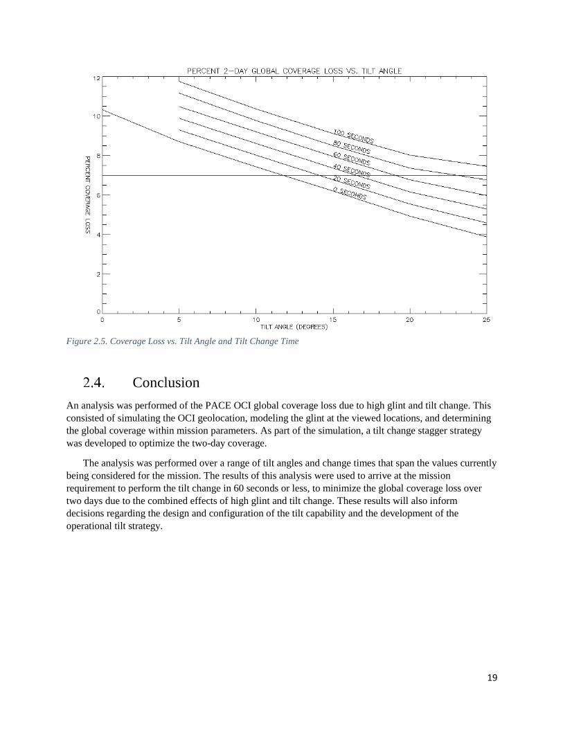
and change time, following the same steps as described in Section II. The results are shown in Figure 2.5;

coverage loss of 7%, approximately the annual average for a 60-second tilt change time, is shown as the

horizontal line on the plot.

The figure shows that the time allowed for the tilt change decreases rapidly as the tilt angle decreases,

in order to maintain a given coverage loss. This is due to the rapid increase in the area affected by high

glint at lower tilt angles, even though the tilt change gap is also reduced. The figure also shows an

additional reduction in coverage loss for a tilt angle of 25 degrees, although the improvement is less than

that seen between 15 and 20 degrees.

19

Figure 2.5. Coverage Loss vs. Tilt Angle and Tilt Change Time

Conclusion

An analysis was performed of the PACE OCI global coverage loss due to high glint and tilt change. This

consisted of simulating the OCI geolocation, modeling the glint at the viewed locations, and determining

the global coverage within mission parameters. As part of the simulation, a tilt change stagger strategy

was developed to optimize the two-day coverage.

The analysis was performed over a range of tilt angles and change times that span the values currently

being considered for the mission. The results of this analysis were used to arrive at the mission

requirement to perform the tilt change in 60 seconds or less, to minimize the global coverage loss over

two days due to the combined effects of high glint and tilt change. These results will also inform

decisions regarding the design and configuration of the tilt capability and the development of the

operational tilt strategy.

20

Chapter 3

Case Study on the Science Data Completeness

Requirement for PACE

Jeremy Werdell, NASA Goddard Space Flight Center, Greenbelt, Maryland3

3.

Executive Summary

This case study defines the science data completeness requirement for the Plankton, Aerosol, Cloud,

ocean Ecosystem (PACE) Ocean Color Instrument (OCI). The mission adopted a >93.33% data

completeness requirement, with data completeness defined as normal operations of the OCI (e.g., versus

time spent in safe hold) and held separately from the Level-1 requirement for two-day global coverage.

The 99.33% corresponds to allowing <2-days of data loss per month on average, which is sufficient to

meet PACE Level-1 requirements related to data product generation and their associated uncertainties.

Introduction

Resolving critical ocean basin- and climate-scale science questions requires complete global maps on

weekly and monthly time scales, respectively. Note that other regional science questions (e.g., upwelling

zones, at frontal boundaries, and in tidal estuaries) require much finer temporal resolution, but do not

drive the prime science of this mission and do not appear as considerations in this study (see, e.g., the

PACE Science Definition Team report [2018]) An instrument that avoids contamination by Sun glint

(normally accomplished by tilting) with two-day global coverage and a ground sample distance (GSD) of

no more than 1000 m at nadir provides the best-known polar-orbiter configuration for achieving the

temporal and spatial scales required to address basin- and climate-scale science questions. OCI will likely

achieve this configuration, however, the question remains as to how often it can fail to collect data and

still meet the science requirements for the mission.

Analysis

3.2.1. A Review of Global Ocean Color Retrievals

The case study presented here defines the science data completeness requirement for OCI in terms of

allowable days lost each month. In this study, two heritage satellite instruments are considered: (1)

SeaWiFS, which tilted to avoid Sun glint and provided 9-km global maps; and (2) MODISA, which does

not tilt and provides 4-km global maps.

3 Cite as: Werdell, P. J. (2018), Case study on the science data completeness requirement for PACE, in PACE Technical Report



21

Figure 3.1: Two days of SeaWiFS data and their two-day composite (9-km). Black pixels indicate either land or

missing data due to clouds, atmospheric aerosols, and Sun glint.

Despite the truncation of SeaWiFS Global Area Coverage (GAC) data at ±45o (unlike MODISA and

OCI, which will provide data to ~58o), SeaWiFS provides the best example to illustrate the anticipated

OCI coverage because it tilted to avoid Sun glint (Figure 3.1). While SeaWiFS had two-day coverage (all

Earth pixels were viewed at least once every two days) and minimized the loss of pixels due to Sun glint,

ocean retrievals were still missed. Ocean color retrievals are limited by the presence of clouds, substantial

atmospheric aerosols, and Sun glint. PACE is a multi-discipline mission encompassing clouds, aerosols,

and ocean color, however, cloud or aerosol retrievals have fewer limiting factors. As such, ocean

retrievals are considered to be the driving requirement for data completeness within this study.

3.2.2. Analysis of Data Completeness

MODISA is used in the remainder of this analysis, as it provides a GSD similar to OCI and, therefore,

best illustrates the 4-km spatial compositing expected to be applied to PACE. Figure 3.2 shows

chlorophyll-a (a standard ocean color product) from MODISA composited to 7, 14, 21, and 31 days.

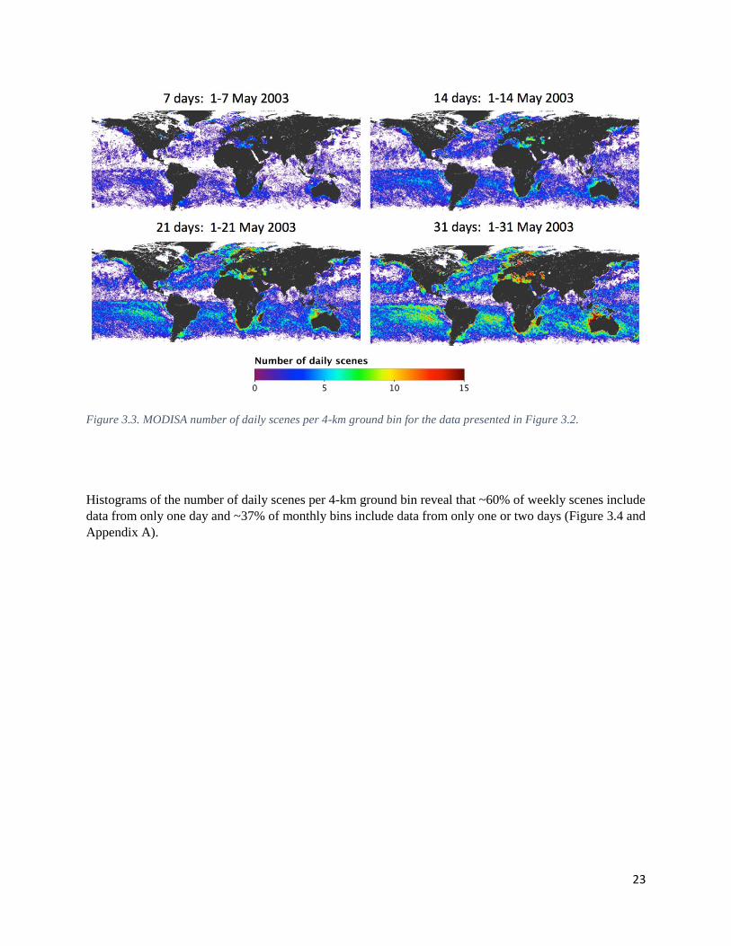
Figure 3.3 shows the number of daily scenes (N) included in each 4-km ground bin.

22

Figure 3.2. MODISA 4-km chlorophyll-a composites. Black pixels defined as in Figure 3.1.

Spatially, the monthly composites are not completely filled and many monthly bins include data from

only one or two days. Many of the losses near the Equator are due to Sun glint. OCI is expected to

recover those pixels by tilting and the number of observations shown in Figure 3.3 near the Equator will

mimic those at higher latitudes. That is, in most cases N=1 will become N>1 and the maps will fill

similarly to what is shown for SeaWiFS in Figure 3.1. While not the primary purpose of this study, the

use of MODISA in this analysis also illustrates the data completeness impacts of not tilting to avoid Sun

glint.

23

Figure 3.3. MODISA number of daily scenes per 4-km ground bin for the data presented in Figure 3.2.

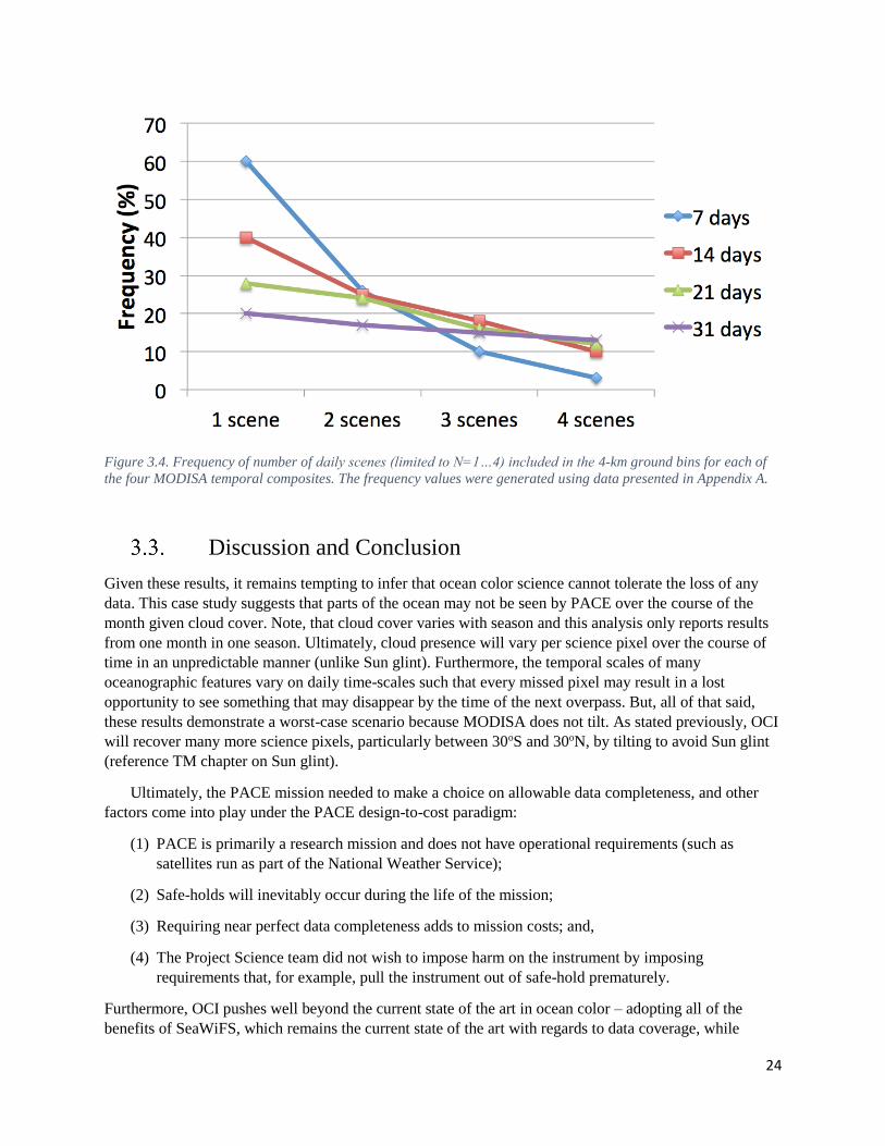
Histograms of the number of daily scenes per 4-km ground bin reveal that ~60% of weekly scenes include

data from only one day and ~37% of monthly bins include data from only one or two days (Figure 3.4 and

Appendix A).

24

Figure 3.4. Frequency of number of daily scenes (limited to N=1…4) included in the 4-km ground bins for each of

the four MODISA temporal composites. The frequency values were generated using data presented in Appendix A.

Discussion and Conclusion

Given these results, it remains tempting to infer that ocean color science cannot tolerate the loss of any

data. This case study suggests that parts of the ocean may not be seen by PACE over the course of the

month given cloud cover. Note, that cloud cover varies with season and this analysis only reports results

from one month in one season. Ultimately, cloud presence will vary per science pixel over the course of

time in an unpredictable manner (unlike Sun glint). Furthermore, the temporal scales of many

oceanographic features vary on daily time-scales such that every missed pixel may result in a lost

opportunity to see something that may disappear by the time of the next overpass. But, all of that said,

these results demonstrate a worst-case scenario because MODISA does not tilt. As stated previously, OCI

will recover many more science pixels, particularly between 30oS and 30oN, by tilting to avoid Sun glint

(reference TM chapter on Sun glint).

Ultimately, the PACE mission needed to make a choice on allowable data completeness, and other

factors come into play under the PACE design-to-cost paradigm:

(1) PACE is primarily a research mission and does not have operational requirements (such as

satellites run as part of the National Weather Service);

(2) Safe-holds will inevitably occur during the life of the mission;

(3) Requiring near perfect data completeness adds to mission costs; and,

(4) The Project Science team did not wish to impose harm on the instrument by imposing

requirements that, for example, pull the instrument out of safe-hold prematurely.

Furthermore, OCI pushes well beyond the current state of the art in ocean color – adopting all of the

benefits of SeaWiFS, which remains the current state of the art with regards to data coverage, while

25

increasing its composited spatial resolution from 9-km to 4-km. OCI is expected to ultimately provide the

best ever global data coverage for the ocean color community.

Given the above and with conscientious consideration of mission costs, the PACE mission adopted

the data completeness requirement of >93.33%, which translates to an allowable data loss of <2-days per

month. While this recommendation does not strictly follow the results presented in this case study,

increasing this requirement to 95% would have added substantial financial burden that could not be

tolerated under design-to-cost.

The recommended data completeness requirement does not substantially impact the PACE mission’s

ability to meet any Level-1 science requirement. The most relevant Level-1 requirement to this study

remains the uncertainties assigned to science data products. Achievement of these uncertainties will be

verified using coincident satellite-to-in situ match-ups using satellite data processed only to Level-2 (daily

science data products from Level-1B; neither spatially or temporally composited). Following, data

completeness only comes in to play by potentially extending the time period over which one accumulates

a statistically relevant number of satellite-to-in situ match-ups. Given that many in situ data sources

collect data autonomously on daily scales, extending this time period is not expected to substantially deter

accumulating match-ups over the 18-month threshold mission life. As a thought exercise, consider that

MODISA achieved ~240 match-ups in 2007, or roughly 20 match-ups per month. If only 90% of these

match-ups were possible because of 10% loss of MODISA data, we would be left with an average of 18

match-ups per month, or 216 total, a sufficiently robust sample size for evaluation of instrument

performance.

Finally, this recommended data completeness requirement is not intended to compete with or violate

the Level-1 requirement for 2-day global coverage, the intent for which is to offer an opportunity to

retrieve a valid ocean color, aerosol, or cloud data product globally every 2-days under normal operating

conditions.

26

Appendix A.

This appendix provides frequency and cumulative distributions of the number of daily scenes per 4-km

ground bin for four MODISA temporal composites, used to generate Figure 3.4.

27

28

Chapter 4

Assessment of Hyperspectral Pushbroom Image Striping

Artifacts in Ocean Color Products

Lachlan I. W. McKinna, Go2Q Pty Ltd, Buderim, Australia 4

Robert Lossing, Science Applications International Corporation, Reston, VA

Jeremy Werdell, NASA Goddard Space Flight Center, Greenbelt, Maryland

4.

Executive Summary

For pushbroom imaging spectroradiometers, detector-to-detector miscalibration error can cause along-

track image striping artifacts. During the pre-Phase A period of the Plankton, Aerosol, Cloud, ocean

Ecosystem (PACE) mission, a pushbroom imager design concept was considered for the Ocean Color

Instrument (OCI). In this chapter, striping artifacts in the MERIS pushbroom ocean color data were

examined, the affects striping artifacts have on science data products were assessed, and the feasibility of

‘destriping’ pushbroom imagery was considered. Collectively these analyses indicate that a pushbroom

instrument would propagate striping artifacts through to ocean color data products causing unwanted

uncertainty that may not be easily corrected out using destriping algorithms.

Introduction

The pushbroom sensor design is common in passive optical remote sensing. The sensor comprises a linear

array of photodetectors that simultaneously image m cross-track pixels as the spacecraft progresses

forward [McClain et al., 2014]. For hyperspectral observations, an optical dispersion element (e.g. a

grating) is typically used to split the observed optical beam into n spectral bands that are then projected

onto the focal plane. Thus, a pushbroom sensor with m spatial pixels and n spectral bands requires a focal

plane with n x m individual detectors.

Each individual pushbroom detector requires characterization and its own calibration coefficients. For

a given spectral band, miscalibration of one or more detector elements can lead to those detectors

recording cross-track radiances at intensities different to adjacent cross track pixels. This effect causes

distinct along-track lines in imagery commonly referred to as “image striping” as shown in Figure 4.1.

Similar to noise, striping artifacts are propagated through data processing algorithms, including

atmospheric correction, into derived data products such as water-leaving reflectances (ρw) and inherent

optical properties (IOPs).

Amongst early design guidelines for the OCI during the PACE Mission’s pre-Phase A period was the

following criteria for top-of-atmosphere radiometry:

4 Cite as: McKinna, L. I. W., R. Lossing, and J. Werdell (2018), Assessment of hyperspectral pushbroom image striping artifacts

in ocean color products, in PACE Technical Report Series, Volume 5: Mission Formulation Studies (NASA/TM-2018 – 2018-

219027/ Vol. 5), edited by I. Cetinić, C. R. McClain and P. J. Werdell, NASA Goddard Space Flight Space Center Greenbelt,

MD.

29

Image striping artifacts, which result from uncharacterized differences in detector responsivity,

that are <0.5% and correctable to noise levels

Accordingly, a study was scoped to assist in determining the likely impact pushbroom striping

artifacts would have upon derived science data products. This chapter is a collection of four case studies:

(i) investigating the magnitude of striping artifacts in heritage MERIS pushbroom sensor data, (ii)

assessing the impact of striping artifacts on derived science data products, (iii) assessing the impact of

striping artifacts on a novel derivative spectroscopy method, and (iv) considering the effectiveness of

destriping methods at correcting striping to sensor noise levels. The latter three analyses relied on a

simplified model for a hyperspectral pushbroom sensor in which detector miscalibration error could be

defined.

Figure 4.1: MERIS imagery of the Gulf of Mexico region captured on 13 December 2004. (A.) A quasi-true color

image in which distinct vertical contrast boundaries are visible associated with where the sensor’s five individual

cameras overlap. (B.) An image of derived remote sensing reflectances at 413 nm, Rrs(413), with a red zoom box.

(C.) The zoomed-in region shows vertical along-track image striping in Rrs(413) which are delineated more clearly

in (D.) using vertical red lines.

Heritage Instrument Data

The MERIS instrument, flown aboard ESA’s ENVISAT (2002-2012), comprised five separate

pushbroom cameras, each with a backlit silicon frame transfer charge coupled device (CCD) focal plane

having 740 spatial pixels and 520 spectral pixels [Bézy et al., 2000]. Thus, the number of total detectors

elements on the MERIS pushbroom system was 1.924x106 (5 x 520 x 740). The MERIS sensor exhibited

three distinct along-track striping artifacts:

30

Detector-to-detector miscalibration

Miscalibrations cause pixel-to-pixel contrast variations and appear as along-track stripe artifacts as

the scene is built up due to the push broom motion.

Between-camera discontinuities

The radiometric contrast between the sensor’s five separate cameras varies. This causes distinct

vertical boundaries where each sub-image overlaps.

Dead detector interpolation

Non-functional, or “dead”, detectors on the CCD focal plane can occur due to aging and/or

manufacturer fault. Once identified, dead pixels are replaced by interpolating between adjacent detectors.

These appear as along-track stripes similar to those caused by detector-to-detector miscalibration.

A cursory evaluation of along-track striping artifacts in MERIS imagery was performed using an

image of the South Atlantic Gyre captured on 12 March 2009. Near-surface waters within a sub-tropical

gyre are oligotrophic and can be treated quasi-homogenous at local horizontal scales. Such a region was

thus useful for evaluating along-track striping artifacts in spectral top-of-atmosphere radiances, Ltoa(λ), as

the magnitude of an identified stripe can be compared with adjacent pixels to ascertain its deviation from

the neighborhood value.

Ltoa(λ) stripes occurring at cross-track pixel number 229 and 645 were evaluated. For each stripe, a 60

pixel-long along-track region-of-interest was considered. Immediately either side of the stripe two boxes

20 pixels wide and 60 pixels long (see Figure 4.2) were averaged and then compared with the average of

the 60 pixel-long image stripe. The metric used for comparison was the relative percent difference.

Similarly, the difference between cameras 3 and 4 and cameras 4 and 5 were computed. Specifically, two

boxes 40 pixels wide and 60 pixels (see Figure 4.2) were averaged either side of each camera seam and

then the relative percent difference (RPD) was calculated.

Figure 4.2A shows a striping artifact in top-of-atmosphere radiances at 443 nm, Ltoa(443), for cross-

track pixel number 229. The RPD between this stripe and neighboring pixels was 0.50%. The spectral

results detailed in Table 4.1 and shown in Figure 4.2 indicate that image striping artifacts in Ltoa differed

from neighborhood values by ±0.5% or more on five occasions. Figure 4.2B shows the difference

between cameras 4 and 5 in top-of-atmosphere radiances at 443 nm, Ltoa(443). The relative percent

difference between cameras was 0.18% with full spectral results presented in Table 4.2 and shown in

Figure 4.4 indicating.

The results shown in Figures 4.2 and 4.3 and summarized in Tables 4.1 and 4.2 indicate that striping

artifacts exceeded the ±0.5% error threshold on four occasions. Whereas, cameras seam edges exceeded

the ±0.5% threshold on twelve occasions. We note that these results comes after much post-processing to

remove detector-to-detector artifacts by Bouvet and Ramino [2009].

31

Figure 4.2: Subplots from a MERIS image captured over the South Atlantic Gyre on 12 March 2009. (A) An

example of a miscalibration stripe in Ltoa(443) occurring at cross track pixel number 229. The magnitude of the

stripe was compared with adjacent pixels for a box 20 pixels wide and 60 pixels long. (B) Comparison of MERIS

cameras 4 and 5 at Ltoa(443). The magnitude of the difference between adjacent cameras was calculated by

comparing the average pixel values either side of the seam for a test region 40 pixels wide and 60 pixels long.

Figure 4.3: For miscalibration stripes occurring at cross-track pixels 229 and 645, the relative percent difference

(RPD) between the stripe and the neighboring region was calculated for each spectral band. The shaded grey box

represents ±0.5% difference.

32

Figure 4.4: The relative percent difference (RPD) was computed at the seams of cameras 3 and 4 and cameras 4

and 5. RPD were calculated for each spectral band. The shaded grey box represents ±0.5% difference.

Pushbroom Conceptual Model

A basic model was developed to conceptualize image striping in a contiguous multispectral pushbroom

ocean color sensor analogous to MERIS with 14-bit digitization resolution. The theoretical CCD focal

plane had n=740 spatial pixels and m=83 spectral bands (340 - 750 nm, 5 nm resolution). Within the

scope of this study, the theoretical sensor was assumed to be ideal (i.e. no other artifacts) with at-launch

noise levels as determined from prescribed signal-to-noise ratios (SNRs) in the PACE Science Definition

Team (SDT) Report and random calibration uncertainties that were adjustable.

The model first calculates hypothetical top-of-atmosphere sensor-observed digital counts for the ith

spatial and jth spectral detector, DNi,j, as follows:

1. A simple bio-optical model was used to generate spectral remote sensing reflectance for each

spatial pixel, Rrsi,j, as a function of chlorophyll-a, Chli, concentration.

2. Theoretical Rrsi,j was converted to water leaving radiances, Lwi,j, by multiplying by an idealized

down-welling spectral irradiance constant, Edj.

3. An idealized atmospheric spectral radiance constant, Latmj, was added to Lwi,j to generate top-of-

atmosphere radiances, Ltoai,j. Based on Sea-Viewing Wide-Field-of-View Sensor (SeaWiFS) data

captured over the North Pacific Ocean near Hawaii, the following power law relationship was

used to approximate Latmj

Latmj= Latm

555

555

lj

æ

èç

ö

ø÷

4

. (Eq. 4.1)

where, λj, is jth sensor spectral band center wavelength and the atmospheric radiance at 555,

Latm555, was set to 2.5 mW cm-2 um-1 sr-1.

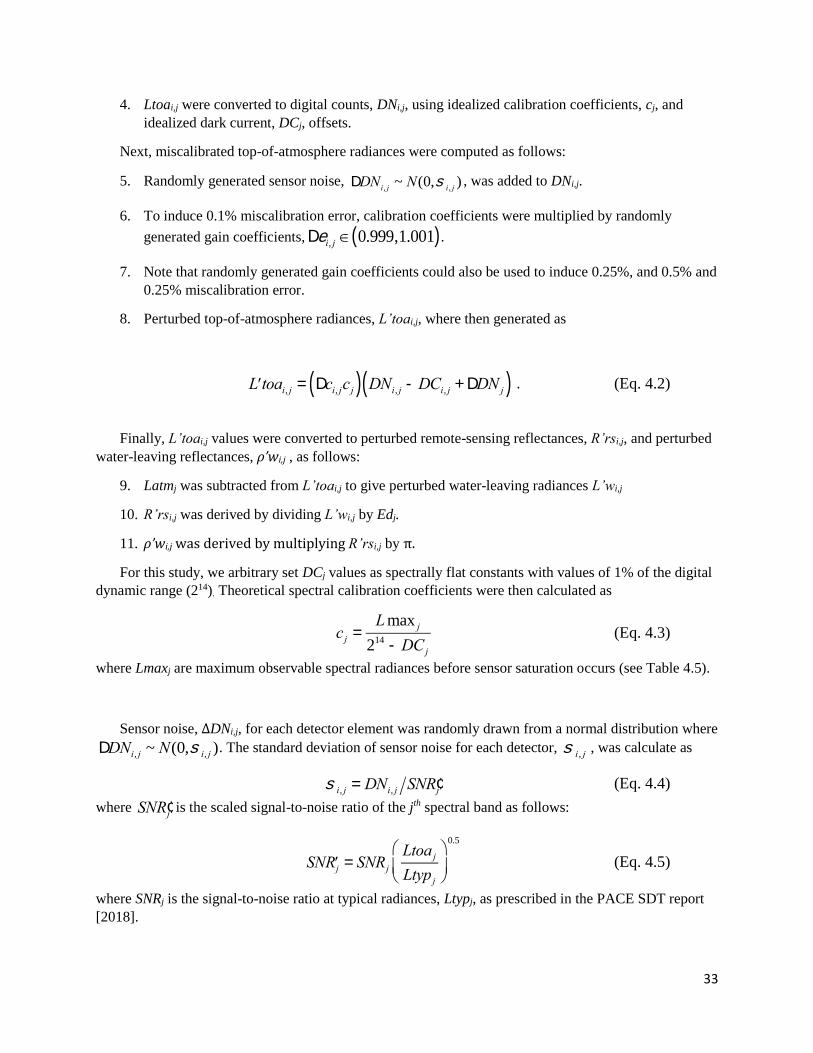
33

4. Ltoai,j were converted to digital counts, DNi,j, using idealized calibration coefficients, cj, and

idealized dark current, DCj, offsets.

Next, miscalibrated top-of-atmosphere radiances were computed as follows:

5. Randomly generated sensor noise, DDNi, j

~ N(0,si, j

) , was added to DNi,j.

6. To induce 0.1% miscalibration error, calibration coefficients were multiplied by randomly

generated gain coefficients, Dei, j Î 0.999,1.001( ).

7. Note that randomly generated gain coefficients could also be used to induce 0.25%, and 0.5% and

0.25% miscalibration error.

8. Perturbed top-of-atmosphere radiances, L’toai,j, where then generated as

¢L toai, j = Dci, jc j( ) DNi, j - DCi, j + DDN j( ) . (Eq. 4.2)

Finally, L’toai,j values were converted to perturbed remote-sensing reflectances, R’rsi,j, and perturbed

water-leaving reflectances, ρ’wi,j , as follows:

9. Latmj was subtracted from L’toai,j to give perturbed water-leaving radiances L’wi,j

10. R’rsi,j was derived by dividing L’wi,j by Edj.

11. ρ’wi,j was derived by multiplying R’rsi,j by π.

For this study, we arbitrary set DCj values as spectrally flat constants with values of 1% of the digital

dynamic range (214). Theoretical spectral calibration coefficients were then calculated as

c j =L max j

214 - DC j

(Eq. 4.3)

where Lmaxj are maximum observable spectral radiances before sensor saturation occurs (see Table 4.5).

Sensor noise, ΔDNi,j, for each detector element was randomly drawn from a normal distribution where

DDNi, j ~ N(0,s i, j ). The standard deviation of sensor noise for each detector, s i, j , was calculate as

s i, j = DNi, j SN ¢Rj(Eq. 4.4)

where SN ¢Rjis the scaled signal-to-noise ratio of the jth spectral band as follows:

SN ¢Rj = SNRj

Ltoa j

Ltyp j

æ

èç

ö

ø÷

0.5

(Eq. 4.5)

where SNRj is the signal-to-noise ratio at typical radiances, Ltypj, as prescribed in the PACE SDT report

[2018].

34

The quasi-single scattering approximation of Gordon et al. [1988] was used to simulate Rrsi,j. For the

ith spatial pixel, the spectral sub-surface remote sensing reflectance was modeled as

rrs j = 0.089u j + 0.125u j

2 . (Eq. 4.6)

Subsurface to above-water values were converted following Lee et al. [2002] as

Rrs j =0.52rrs j

(1-1.7rrs j ) . (Eq. 4.7)

The spectral parameter uj is a function of the total spectral absorption coefficient, aj, and the total

spectral backscattering coefficient, bb,j, expressed as

u j =a j

a j + bb, j

. (Eq. 4.8)

Values of aj and bb,j were modeled as functions of Chl following IOCCG [2006]. However, unlike

IOCCG [2006], the spectral absorption coefficient of phytoplankton, a,j, was parameterized according to

Bricaud et al. [1998].

Example of Synthesized Pushbroom Striping

Simulated ρw(440) images that are 740 pixels (cross-track) wide and 500 pixels (along-track) long are

shown in Figures 4.5A and 4.5B. The two images represent a uniform ocean with Chl value of 0.1 mg m-3

“imaged” by the conceptual pushbroom model. Figure 4.5A is modeled with 0.1% miscalibration error

whilst Figure 4.5B is modeled with 0.1% miscalibration error and sensor noise. Along-track striping

artifacts are clearly visible in both subplots. The addition of noise to the model introduces a speckle

characteristic that qualitatively appears similar to MERIS imagery.

Figures 4.5C and 4.5D show cross-track transects of ρw(440) corresponding to scanline 100 (denoted

as red lines in Figure 5A and 5B). Relative percent difference (RPD) values in Figure 4.5C indicate that

0.1% miscalibration error causes values of ρw(440) to vary ±0.8% from the mean value. Whereas,

Figure 4.5D shows that miscalibration error and sensor noise cause values of ρw(440) to vary ±3%

from the mean value.

Figures 4.5E and 4.5F show the actual spectral value of ρw(λ) for the simulated scene. The gray

shaded area surrounding ρw(λ) represents ±1σ(λ) computed from all ρw(λ) in the simulated image. The

blue line represents the spectral mean absolute percent difference (MAPD) deviation from true

ρw(λ) and the horizontal dashed lines represents a 0.5% MAPD. Here, MAPD was calculated as:

MAPD =¢rw

- rw

¢rw

æ

èç

ö

ø÷ ´100% (Eq. 4.9)

where, 𝜌𝑤′ is the miscalibrated water leaving reflectance value (wavelength has been omitted for brevity).

We note that in this study, atmospheric correction was treated as an exact subtraction of modeled

Latm(λ) from Ltoa(λ). In practice, however, atmospheric correction uses near-infrared channels to estimate

atmospheric parameters. Accordingly, this study did not capture how striping artifacts from near-infrared

channels might propagate through to shorter wavelengths during the atmospheric correction procedure.

35

Figure 4.5: Subplots (A) and (B) show simulated pushbroom images of ρw(440) for a uniform ocean: (A) is modeled

with 0.1% miscalibration error, and (B) is modeled with 0.1% miscalibration error in the presence of noise.

Subplots (C) and (D) show variability in ρw(440) along a cross-track transect for scan number 100 (denoted as

redlines in subplots (A) and (B)). Subplots (E) and (F) show the true ρw(λ) and the transect-averaged spectral mean

absolute percent differences (MAPD).

Impact of Striping on Derived Products

The impact of miscalibration error upon derived ocean color data products was explored using a

synthesized ocean scene of a bio-optical gradient. Four hyperspectral pushbroom images were simulated:

(i) for a well-calibrated sensor, (ii) for a sensor with 0.1% miscalibration error, (iii) for a sensor with

0.25%, and (iv) for a sensor with 0.5% miscalibration. Further, identical sensor noise characteristics were

used for all three scenarios. The relative error, δDP, between the value of the data product derived from

the perfectly calibrated sensor, DP, and the data product derived from the miscalibrated sensor, DP’, was

calculated as follows:

d Dp =D ¢P - DP

DP

é

ëê

ù

ûú ´100% . (Eq. 4.10)

Chl values were derived using the OC4 band ratio-type algorithm [O'Reilly et al., 1998] and inherent

optical properties (IOPs) at 440 nm were derived using the default configuration of the Generalized

Inherent Optical Properties algorithm framework (GIOP) [Werdell et al., 2013]. In this study, the IOPs

derived at 440 nm were the absorption coefficient of phytoplankton, aϕ(440), the absorption coefficient of

colored dissolved and detrital matter, adg(440), and the particulate backscattering coefficient, bbp(440).

Figure 4.6A and 4.6B shows aϕ(440) derived for a perfectly calibrated sensor and a sensor with 0.1%

miscalibration error, respectively. In Figure 4.6B, along-track (vertical) miscalibration striping can be

seen in derived aϕ(440). Figure 4.6C is a histogram of δaϕ(440) and shows that 0.1% miscalibration

imparts approximately ±1% 1σ uncertainty in derived aϕ(440). Figure 4.6D is an image of the relative

difference in which along-track (vertical) striping artifacts can be seen.

Table 4.6 summarizes the first standard deviation (1σ) values of δChl, δ aϕ(440), δ adg(440), and

δbbp(440) for the 0.1%, 0.25% and 0.5% miscalibration error scenarios. The results indicate that 1σ

36

uncertainty in derived data products scales nearly linearly with sensor miscalibration (striping) error.

Notably, at the 0.5% miscalibration level the 1σ uncertainty in Chl approaches 10%.

Figure 4.6: Derived aϕ(440) from a simulated hyperspectral pushbroom image of a synthesized non-uniform ocean.

(A) aϕ(440) derived from a well-calibrated sensor, while (B) shows perturbed a’ϕ(440) derived from sensor with

0.1% miscalibration errors and noise. (C) A histogram shows the distribution of the relative difference between (A)

and (B). (D) Shows and image of the relative difference between (A) and (B).

Impact of Striping on Deriviative Spectroscopy

One novel aspect of a hyperspectral OCI is applying analytical spectroscopy methods common to

chemometrics to ocean color data. In particular, derivative spectroscopy methods may lend themselves to

hyperspectral ocean color radiometry for discerning subtle phytoplankton accessory pigment absorption

peaks e.g. [Craig et al., 2006; Lubac et al., 2008; Xi et al., 2015]. Here we briefly considered how

miscalibration error in a pushbroom sensor might impact derivative spectroscopy of hyperspectral ρw(λ).

37

Using the pushbroom conceptual model, a hyperspectral ρw(λ) image was simulated for uniform

ocean with Chl of 1 mg m-1. An image 740 pixels (cross-track) wide and 500 pixels (along-track) long

was simulated for a noiseless sensor with 0.1% miscalibration error. For comparison purposes, ρw(λ) was

modeled again for a noiseless perfectly calibrated sensor.

Figure 4.7A shows an image of the second derivative of ρw(λ) at 513 nm, d2ρw(513)/dλ2. The mean

value of d2ρw(513)/dλ2 is 5.6E-4 nm-2 and ranges from -4.9E-5 to 1.1E-3 nm-2 with a standard deviation of

2.0E-4 nm-2. Figure 4.7B shows the relative comparison of d2ρw(513)/dλ2 values in Figure 4.7A with

d2ρw(513)/dλ2 modeled for a perfect sensor. The results demonstrate that between-pixel variability due to

image striping can be as much as ±120%.

A cross-track sample of spectral d2ρw/dλ2 is shown in Figure 4.7C as well as the true value for ρw(λ).

Second derivative features correspond as expected to spectral curvature features in ρw(λ). It is clear that

absolute uncertainty in ρw(λ) associated with miscalibration error increases as wavelength decreases.

Figure 4.7: (A) An image of d2ρw(515)/dλ2 for a hypothetical uniform ocean. d2ρw(515)/dλ2 was calculated from a

synthesized hyperspectral ρw(λ) image modeled for a noiseless pushbroom sensor with 0.1% miscalibration error.

The horizontal red line denote a cross-track transect at scanline number 50. (B) An image of the relative percent

difference between ideal d2ρw(515)/dλ2 and d2ρw(515)/dλ2 shown in (A). (C) A cross-track sample of d2ρw(515)/dλ2 is plotted showing 1σ variability. The ideal ρw(λ) spectrum for the uniform is also plotted.

Case Study of Destriping Method

A number of destriping algorithms have been developed to suppress along-track striping artifacts in

pushboroom sensors (see examples in Table 4.5). Destriping methodologies vary in complexity and apart

from efforts to suppress detector-to-detector striping artifacts in MERIS Level-1B data by Bouvet and

Ramino [2009] none, to the best of our knowledge, have been implemented in routine global ocean color

processing. We evaluated the wavelet-based method of Pande-Chhetri and Abd-Elrahman [2011] to

ascertain how a computationally efficient destriping algorithm might suppress striping artifacts in modeled

pushbroom ρw(λ).

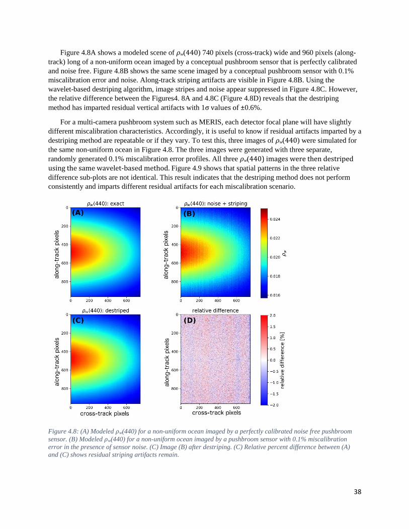
38

Figure 4.8A shows a modeled scene of ρw(440) 740 pixels (cross-track) wide and 960 pixels (along-

track) long of a non-uniform ocean imaged by a conceptual pushbroom sensor that is perfectly calibrated

and noise free. Figure 4.8B shows the same scene imaged by a conceptual pushbroom sensor with 0.1%

miscalibration error and noise. Along-track striping artifacts are visible in Figure 4.8B. Using the

wavelet-based destriping algorithm, image stripes and noise appear suppressed in Figure 4.8C. However,

the relative difference between the Figures4. 8A and 4.8C (Figure 4.8D) reveals that the destriping

method has imparted residual vertical artifacts with 1σ values of ±0.6%.

For a multi-camera pushbroom system such as MERIS, each detector focal plane will have slightly

different miscalibration characteristics. Accordingly, it is useful to know if residual artifacts imparted by a

destriping method are repeatable or if they vary. To test this, three images of ρw(440) were simulated for

the same non-uniform ocean in Figure 4.8. The three images were generated with three separate,

randomly generated 0.1% miscalibration error profiles. All three ρw(440) images were then destriped

using the same wavelet-based method. Figure 4.9 shows that spatial patterns in the three relative

difference sub-plots are not identical. This result indicates that the destriping method does not perform

consistently and imparts different residual artifacts for each miscalibration scenario.

Figure 4.8: (A) Modeled ρw(440) for a non-uniform ocean imaged by a perfectly calibrated noise free pushbroom

sensor. (B) Modeled ρw(440) for a non-uniform ocean imaged by a pushbroom sensor with 0.1% miscalibration

error in the presence of sensor noise. (C) Image (B) after destriping. (C) Relative percent difference between (A)

and (C) shows residual striping artifacts remain.

39

Figure 4.9: The relative percent difference between and destriped and exact values of ρw(440). The subplots

correspond to three separate detector-to-detector 0.1% miscalibration error scenarios.

Summary and Conclusion

In this study we investigated along-track striping in ocean color imagery caused by detector-to-detector

miscalibration in a pushbroom imager. We found that despite much post-launch effort, along-track image

striping artifacts in heritage MERIS imagery can exceed 0.5% in Ltoa. This finding indicates that

calibration and characterization of a multi-camera pushbroom imager is highly challenging.

A conceptual pushbroom model was used to simulate the impact of pushbroom striping on derived

science data products. Using simulated data, we found 0.1% miscalibration error led to 1σ uncertainties in

derived products in the order of ±1%. Uncertainties were also found to scale linearly with miscalibration

error. These uncertainties are directly related to multi-detector miscalibration error and may be reduced

by pursuing a sensor design concept with fewer detectors.

Examination of second derivative spectroscopy found the method was highly sensitive to image

striping. The results showed that image striping imparted by 0.1% miscalibration error led to ±120%

uncertainty in the second derivative of ρw(513). This result suggests that a pushbroom imager concept

may limit the application of novel spectroscopy-type methods.

An algorithm for removing image striping was evaluated. The approach was found to cosmetically

remove along-track image stripes, however, on closer inspection the method imparted residual artifacts. It

was also ascertained that the destriping method did not impart residual artifacts in a repeatable way. This

study suggests that for a pushbroom imager concept, significant effort would need to be expended on

developing a robust destriping methodology suitable for global ocean color processing.

40

Table 4.1: Relative percent difference (RPD) in top-of-atmosphere radiometric quantities between along-track

MERIS stripe artifacts and the immediate neighborhood. Two stripes were considered from an image of the South

Atlantic Gyre captured on 12 March 2009. Test stripes correspond to cross-track pixels 229 and 645.

Band Ltoa RPD at pixel

229 [%]

Ltoa RPD at pixel

645 [%]

413 -0.33 0.21

443 -0.50 0.63

490 -0.31 0.16

510 -0.28 0.13

560 -0.51 0.26

620 -0.34 0.31

665 -0.06 0.21

681 -0.73 -0.05

709 -0.55 -0.26

754 -0.45 -0.04

762 -0.35 0.27

779 -0.27 0.17

865 -0.15 0.08

885 0.38 0.14

900 -0.03 -0.48

Table 4.2: Relative percent difference (RPD) in top-of-atmosphere radiometric quantities calculated at MERIS

camera seams. RPD between cameras 4 and 3, and 5 and 4 were considered for a test image of the South Atlantic

Gyre captured n the 12 March 2009.

Band Ltoa Cameras 4-3

[%]

Ltoa Cameras 5-4

[%]

413 0.71 -0.81

443 0.23 0.18

490 -0.01 -0.26

510 0.23 -0.62

560 0.05 -0.07

620 0.28 -0.04

665 0.38 -0.37

681 0.47 -0.78

709 0.33 -0.99

754 0.20 -0.30

762 -0.84 0.59

779 0.58 -0.98

865 -0.15 -0.17

885 -0.94 -0.19

900 -0.95 0.59

41

Table 4.3: Spectral parameters used for image striping model

Nominal band

center [nm]

Band width

[nm]

SNR Ed

[mW m-2

um-1]

Latm

[mW cm-2

um-1 sr-1]

Ltyp

[mW cm-2

um-1 sr-1]

Lmax

[mW cm-2

um-1 sr-1]

350 15 300 61.05 15.81 7.46 35.5

360 15 1000 65.80 14.12 7.22 37.6

385 15 1000 63.81 10.79 6.11 38.1

412 15 1000 118.66 8.23 7.86 60.2

425 15 1000 112.63 7,27 6.95 58.5

443 15 1000 128.15 6.16 7.02 66.4

460 15 1000 136.88 5.30 6.83 72.4

475 15 1000 143.91 4.66 6.19 72.2

490 15 1000 145.69 4.11 5.31 68.6

510 15 1000 137.50 3.51 4.58 66.3

532 15 1000 137.96 2.96 3.92 65.1

555 15 1000 136.31 2.50 3.39 64.3

583 15 1000 134.71 2.05 2.81 62.4

617 15 1000 121.26 1.63 2.19 58.2

640 10 1000 120.65 1.41 1.90 56.4

655 15 1000 111.94 1.29 1.67 53.5

665 10 1000 117.47 1.21 1.60 53.6

678 10 1000 115.62 1.12 1.45 51.9

710 10 1000 104.50 0.93 1.19 48.9

748 15 600 99.47 0.76 0.93 44.7

Table 4.4: Relative error in derived bio-optical data products imparted by miscalibration error in the conceptual

pushbroom imager model.

Pushbroom

miscalibration

error [%]

1-σ relative percent error [%]

δChl δaϕ(440) δadg(440) δbbp(440)

0.1 1.7 1.1 1.2 0.7

0.25 4.5 2.7 3.0 1.9

0.5 8.9 5.6 6.2 3.9

42

Table 4.5: Selection of along-track destriping methodologies for pushbroom imagery

Technique

Evidence of use

in automated

operational

processing

Residual

striping/artifacts

Algorithm

complexity Test sensor/s Reference

Polynomial

fitting ✖ ✔ Low

MOS Franz [1998]

Heterogeneous

single image-

based band

equalization

✖ ✔ Low OCM Lyon [2009]

2D Wavelet

Fourier-

adaptive

filtering

✖ ✔ Moderate Hyperion

Pande-Chhetri and Abd-

Elrahman [2011]

Pande-Chhetri and Abd-

Elrahman [2013]

Homogenous

multiple image-

based band

equalization

✖ ✔ Moderate-to-high MOS

MERIS

Corsini et al. [2000]

Bouvet and Ramino

[2009]

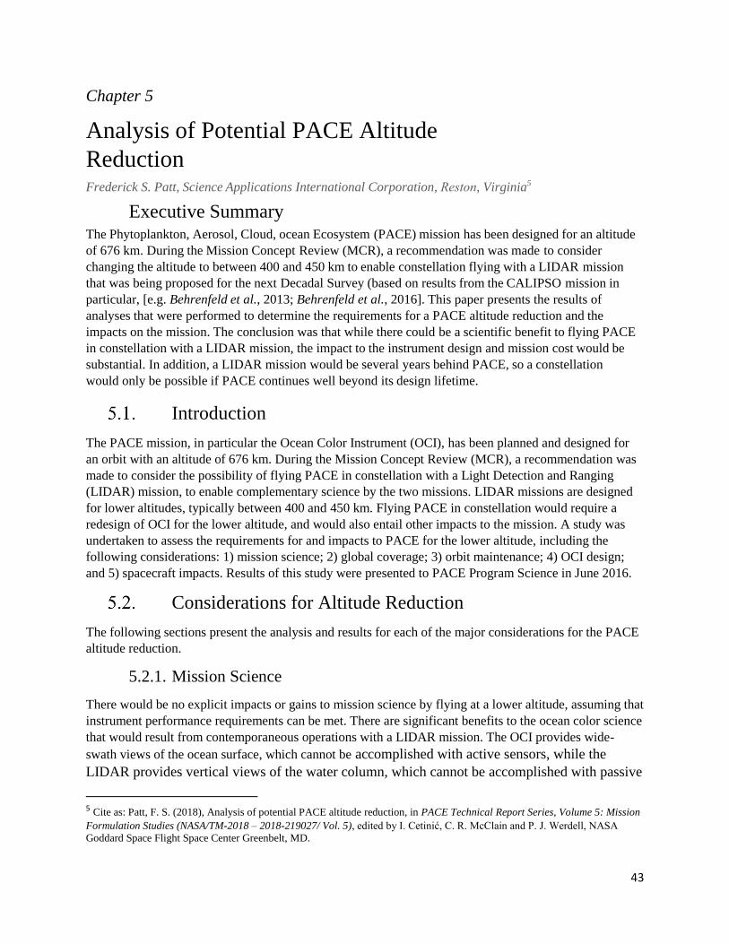
43

Chapter 5

Analysis of Potential PACE Altitude

Reduction Frederick S. Patt, Science Applications International Corporation, Reston, Virginia5

Executive SummaryThe Phytoplankton, Aerosol, Cloud, ocean Ecosystem (PACE) mission has been designed for an altitude

of 676 km. During the Mission Concept Review (MCR), a recommendation was made to consider

changing the altitude to between 400 and 450 km to enable constellation flying with a LIDAR mission

that was being proposed for the next Decadal Survey (based on results from the CALIPSO mission in

particular, [e.g. Behrenfeld et al., 2013; Behrenfeld et al., 2016]. This paper presents the results of

analyses that were performed to determine the requirements for a PACE altitude reduction and the

impacts on the mission. The conclusion was that while there could be a scientific benefit to flying PACE

in constellation with a LIDAR mission, the impact to the instrument design and mission cost would be

substantial. In addition, a LIDAR mission would be several years behind PACE, so a constellation

would only be possible if PACE continues well beyond its design lifetime.

Introduction

The PACE mission, in particular the Ocean Color Instrument (OCI), has been planned and designed for

an orbit with an altitude of 676 km. During the Mission Concept Review (MCR), a recommendation was

made to consider the possibility of flying PACE in constellation with a Light Detection and Ranging

(LIDAR) mission, to enable complementary science by the two missions. LIDAR missions are designed

for lower altitudes, typically between 400 and 450 km. Flying PACE in constellation would require a

redesign of OCI for the lower altitude, and would also entail other impacts to the mission. A study was

undertaken to assess the requirements for and impacts to PACE for the lower altitude, including the

following considerations: 1) mission science; 2) global coverage; 3) orbit maintenance; 4) OCI design;

and 5) spacecraft impacts. Results of this study were presented to PACE Program Science in June 2016.

Considerations for Altitude Reduction

The following sections present the analysis and results for each of the major considerations for the PACE

altitude reduction.

5.2.1. Mission Science

There would be no explicit impacts or gains to mission science by flying at a lower altitude, assuming that

instrument performance requirements can be met. There are significant benefits to the ocean color science

that would result from contemporaneous operations with a LIDAR mission. The OCI provides wide-

swath views of the ocean surface, which cannot be accomplished with active sensors, while the

LIDAR provides vertical views of the water column, which cannot be accomplished with passive

5 Cite as: Patt, F. S. (2018), Analysis of potential PACE altitude reduction, in PACE Technical Report Series, Volume 5: Mission

Formulation Studies (NASA/TM-2018 – 2018-219027/ Vol. 5), edited by I. Cetinić, C. R. McClain and P. J. Werdell, NASA

Goddard Space Flight Space Center Greenbelt, MD.

44

sensors. Wide-swath views of surface processes (OCI) combined with narrow views of vertical

processes (LIDAR) would combine to form a three-dimensional view of the upper ocean (up to 3

optical depths).

However, there are also potential benefits to operating the two missions at the same equator

crossing time but different altitudes. Flying in constellation would result in the LIDAR always

sampling the center of the OCI swath. There may be advantages to having LIDAR measurements

across the full range of OCI scan angles, which would result from different altitudes and orbit

periods. Further study would be required to determine which configuration would provide the

greatest advantages in terms of complementary science.

5.2.2. Global Coverage

PACE has a Level 1 requirement for two-day coverage [Werdell, 2018], within the limit of 60 degrees

sensor zenith angle. Note, this limit only provides a definition for two-day coverage; the OCI will collect

data at larger zenith angles. Note also that data gaps created by OCI tilt maneuvers are not considered in

the definition of global coverage. The 60 degree limit primarily constrains coverage near the equator,

where the one-day inter-orbit gaps are largest. The one-day equatorial coverage is equal to the ratio of the

useful swath width to the orbit track spacing. At the design altitude of 676 km, this coverage is 71.9%.

The coverage changes monotonically with altitude; in the study altitude range of 400 to 450 km, this

figure ranges from 48.9 to 53.6%.

The two-day coverage depends on both the one-day coverage and the overlap between swaths on

successive days. The latter is determined by the number of orbits per day. When this number is an exact

integer, the overlap is 100%, resulting in permanent gaps at the equator, and the two-day coverage is a

minimum. For example, an altitude of about 560 km results in 15 orbits per day. When the number is an

odd number of half-orbits (i.e., a two-day repeat cycle) the coverage from the second day tends to fill the

gaps from the first, and the overall coverage is maximized.

Because the one-day coverage within the study range is close to 50%, maximizing two-day coverage

requires that the orbit be close to a two-day repeat. The orbits per day range from 15.54 at 400 km to

15.37 at 450 km, with 15.5 orbits at 412 km. This suggests that the best two-day coverage will occur close

to 412 km altitude. It should be noted that the data gaps along the equator would be filled by staggering

the times of tilt on successive days as was done during the SeaWiFS mission.

A simulation was performed of two-day coverage within the study altitude range. Two-line elements

(TLEs) were generated for Sun-synchronous polar orbits with a 1:00 pm equator crossing time, for

altitudes from 400 to 450 km at 10-km increments. Orbit ephemeris data were generated for two days

(days 84 and 85 of 2020) at each altitude. OCI geolocation was simulated for the ascending (daylight) part

of the orbit, including a 20-degree fore/aft tilt with a tilt change at the Equator.

Using the simulated geolocation data, the two-day coverage was analyzed for ocean color products.

The useful data were identified based on the mission-specified sensor and solar zenith limits of 60 and 75

degrees, respectively. The viewed locations were then binned at SeaWiFS resolution (9.27 km bins) to

determine global coverage. The two-day coverage for the range of altitudes is illustrated in Figures 5.1

through 5.5.

The simulation confirms that the two-day coverage is maximized between 410 and 420 km altitude. The

global and equatorial coverage is summarized in Table 5.1. (Note that global coverage is also affected by

45

the tilt change data gap.) Within the 410 – 420 km altitude range, the equatorial coverage could be

increased to 100% by redefining the sensor zenith angle limit from 60 to 62 degrees.

It should be noted that a repeat cycle of exactly two days is undesirable for PACE. With this orbit, a given

location will always be viewed at the same scan angle. The science data quality for OCI is improved by

viewing locations at a variety of atmospheric scattering phase angles, particularly when generating Level-

3 temporal composites. Within the study range, an altitude chosen for PACE would represent a

compromise between coverage and the repeat cycle. At the design altitude of 676 km, the orbit repeat

cycle is approximately 11 days.

Figure 5.1. OCI two-day coverage at 400 km altitude.

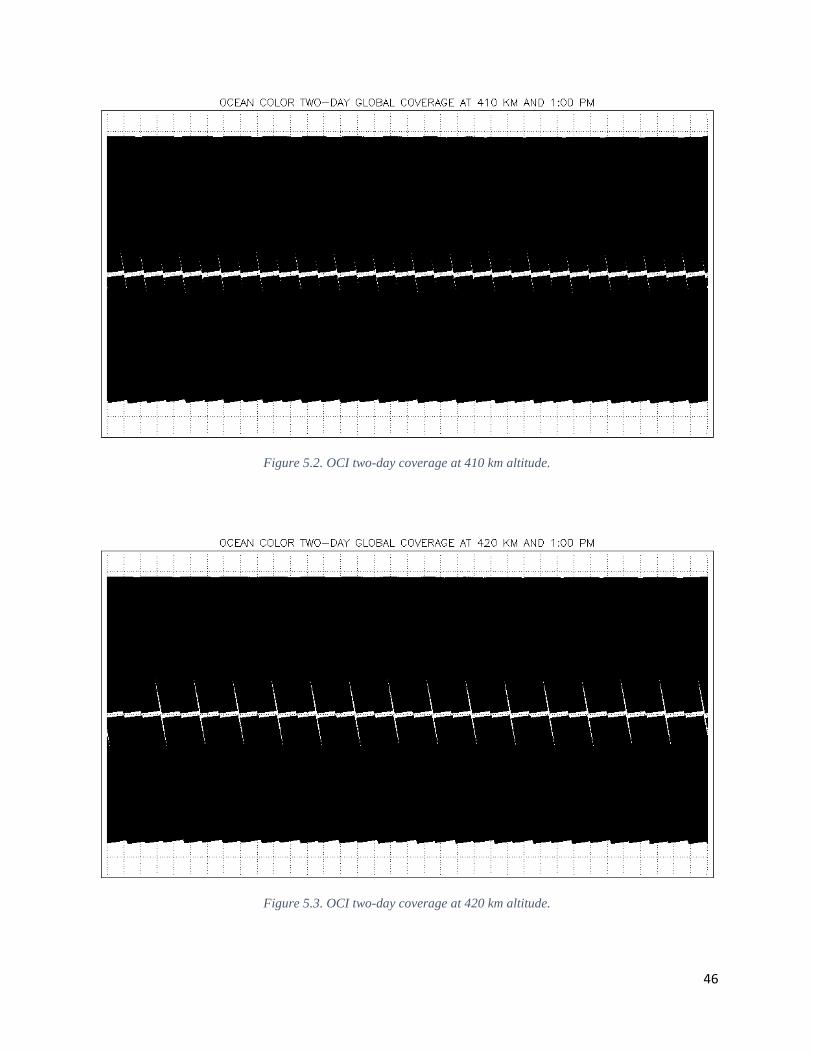
46



47


Figure 5. 5. OCI two-day coverage at 450 km altitude.

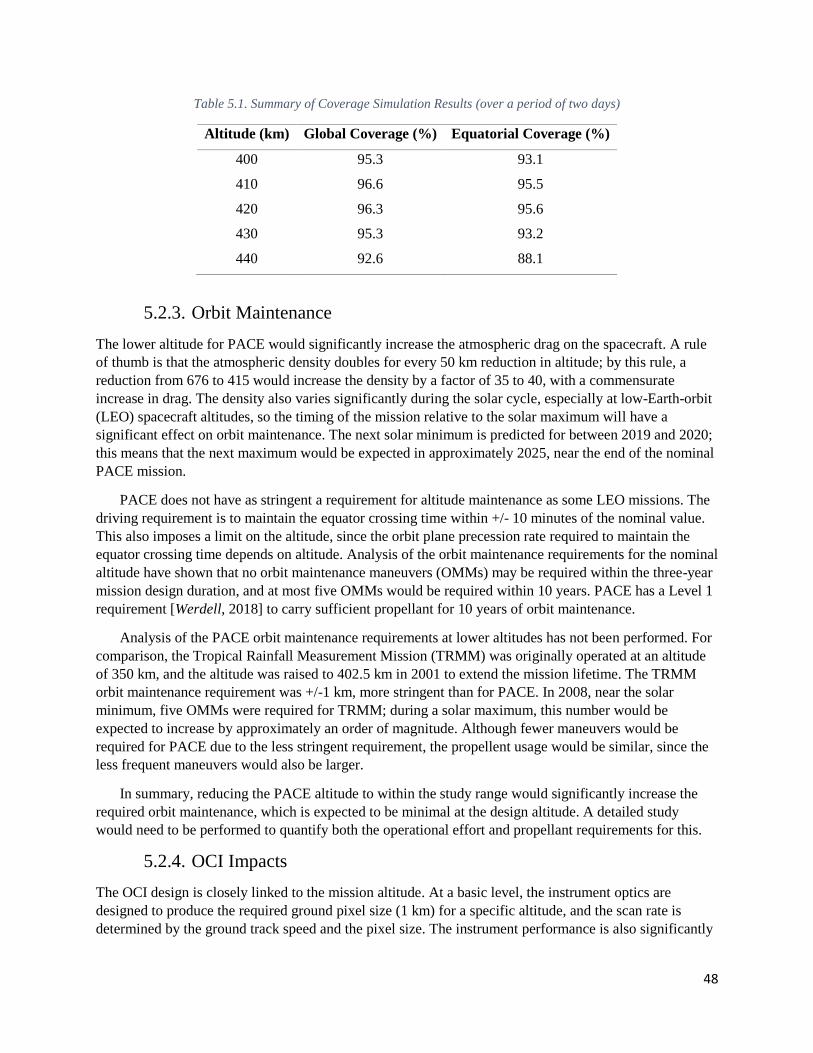
48

Table 5.1. Summary of Coverage Simulation Results (over a period of two days)

Altitude (km) Global Coverage (%) Equatorial Coverage (%)

400 95.3 93.1

410 96.6 95.5

420 96.3 95.6

430 95.3 93.2

440 92.6 88.1

5.2.3. Orbit Maintenance

The lower altitude for PACE would significantly increase the atmospheric drag on the spacecraft. A rule

of thumb is that the atmospheric density doubles for every 50 km reduction in altitude; by this rule, a

reduction from 676 to 415 would increase the density by a factor of 35 to 40, with a commensurate

increase in drag. The density also varies significantly during the solar cycle, especially at low-Earth-orbit

(LEO) spacecraft altitudes, so the timing of the mission relative to the solar maximum will have a

significant effect on orbit maintenance. The next solar minimum is predicted for between 2019 and 2020;

this means that the next maximum would be expected in approximately 2025, near the end of the nominal

PACE mission.

PACE does not have as stringent a requirement for altitude maintenance as some LEO missions. The

driving requirement is to maintain the equator crossing time within +/- 10 minutes of the nominal value.

This also imposes a limit on the altitude, since the orbit plane precession rate required to maintain the

equator crossing time depends on altitude. Analysis of the orbit maintenance requirements for the nominal

altitude have shown that no orbit maintenance maneuvers (OMMs) may be required within the three-year

mission design duration, and at most five OMMs would be required within 10 years. PACE has a Level 1

requirement [Werdell, 2018] to carry sufficient propellant for 10 years of orbit maintenance.

Analysis of the PACE orbit maintenance requirements at lower altitudes has not been performed. For

comparison, the Tropical Rainfall Measurement Mission (TRMM) was originally operated at an altitude

of 350 km, and the altitude was raised to 402.5 km in 2001 to extend the mission lifetime. The TRMM

orbit maintenance requirement was +/-1 km, more stringent than for PACE. In 2008, near the solar

minimum, five OMMs were required for TRMM; during a solar maximum, this number would be

expected to increase by approximately an order of magnitude. Although fewer maneuvers would be

required for PACE due to the less stringent requirement, the propellent usage would be similar, since the

less frequent maneuvers would also be larger.

In summary, reducing the PACE altitude to within the study range would significantly increase the

required orbit maintenance, which is expected to be minimal at the design altitude. A detailed study

would need to be performed to quantify both the operational effort and propellant requirements for this.

5.2.4. OCI Impacts

The OCI design is closely linked to the mission altitude. At a basic level, the instrument optics are

designed to produce the required ground pixel size (1 km) for a specific altitude, and the scan rate is

determined by the ground track speed and the pixel size. The instrument performance is also significantly

49

dependent on the optics and other design parameters that would need to be changed to accommodate an

altitude change.

A preliminary assessment was performed of impacts to the hyperspectral scanning OCI concept due to a

change to a 415 km orbit. The goals were to explore development of a modified OCI concept to support

flying at this altitude, and assess the impact on the signal-to-noise ratio (SNR), a key instrument

performance parameter. These studies were incorporated into an ongoing broader trade on ground sample

distance (GSD) vs SNR.

A specific OCI design, simply placed in a lower orbit without any design modifications, performs

significantly worse in terms of SNR. If the IFOV is not changed, the resulting decrease in GSD results in

decreased signal and decreased SNR. To maintain the baseline SNR, the instantaneous field-of-view

(IFOV) would need to be increased, growing GSD somewhat. The selected GSD was 850 meters. This

would require significant changes to the OCI optical design that, at a minimum, would have resulted in

greater aberration, i.e., an increase in image blurriness. The lower orbit would also require a faster

telescope rotation rate (order ~ 5-6%), increasing loads on the telescope and making alignment more

difficult.

The assessment determined that an additional 4-6 weeks would be required to complete a detailed study

of the optics, opto-mechanical, and mechanism changes required for the lower orbit. Additional technical

obstacles could be uncovered, and study is needed to accurately estimate the additional time required to

perform required design modifications and to understand risks. The OCI engineering team has moved

forward with the baseline 676 km design since the completion of this preliminary assessment.

5.2.5. Spacecraft Impacts

A preliminary assessment was performed of the impacts to the spacecraft design of the lower altitude. In

addition to the orbit maintenance impact, the following potential impacts were noted:

• Increase atomic oxygen (AO) influence: All external surfaces must be AO-resistant. This will

require additional AO blanketing for the backs of solar arrays and other exposed surfaces, and the

use of AO-resistant thermal blanketing, all of which will have mass and cost impacts.

• External optics (e.g, star trackers): Requires additional study to ensure there are no impacts.

• RF communications: The lower orbit will require modification to the earth coverage antenna

(ECA) design and temperature requirements.

• Thermal control: The lower orbit will require an increase in the radiator sizes, which will increase

the cost and mass.

• Guidance, navigation, and control: Higher aerodynamic torques could have minor impact on

some components.

• Mechanical design: Some modification to structure will be required to account for additional

mass.

In addition to the impacts on the spacecraft, it was noted that the reduced altitude could significantly

affect the selection or design of a second instrument, specifically the Multi-Angle Polarimeter (MAP) that

has been proposed for PACE. Existing polarimeter designs that the project understands best are optimized

50

for operation at higher orbits. A 400-450 km orbit could inject significant programmatic risk into the

polarimeter selection.

Conclusion

A study was undertaken of the required changes and potential impacts to the PACE mission of reducing

the mission altitude to 400 – 450 km to operate in constellation with a LIDAR mission. The study

included assessments of mission science, global coverage, orbit maintenance, the OCI design and

performance and the spacecraft design. The following conclusions were reached:

• The direct effect of the altitude change on mission science is neutral. There would be a significant

benefit to contemporaneous operation with a LIDAR mission, but this may also be obtained by

missions at different altitudes.

• Two-day global coverage is marginal at the lower altitude, and limits the altitude range to

between 410 and 420 km.

• Orbit maintenance requirements would be significantly increased at the lower altitude.

• Significant redesign of OCI would be required to meet performance requirements at the lower

altitude, and there are significant risks involved.

• There are multiple potential impacts to the spacecraft; these are manageable but have cost and

possibly schedule impacts.

• The selection of additional instruments (e.g., MAP) will be affected.

In the absence of further direction, the mission design has continued for the 676 km orbit.

51

Chapter 6

PACE OCI Proxy Data Development

Bryan Franz, NASA Goddard Space Flight Center, Greenbelt, Maryland6

6. h

Executive Summary

Prior to the availability of real data from the Ocean Color Instrument (OCI) on PACE, it is useful to have

a source of proxy data for software and algorithm development and testing, e.g., the ocean color

atmospheric correction algorithm and bio-optical property retrieval capabilities. Proxy data is defined

here as real data from another airborne or spaceborne instrument that approximates the OCI spectral

range, such that viable OCI geophysical retrieval algorithms can be operated on the data with minimal

modifications. Data from the hyperspectral AVIRIS instrument [Vane et al., 1993] has been utilized for

this purpose.

Introduction

This document describes the derivation and format of a dataset that may be useful as a proxy for

calibrated top-of-atmosphere radiances that are expected to be provided by the PACE Ocean Color

Instrument (OCI). The proxy data are derived from past airborne campaigns of the Airborne Visible /

Infrared Imaging Spectrometer (AVIRIS) hyperspectral instrument [Vane et al., 1993] and have been

reformatted to match the expected format of a PACE OCI Level-1B file, with the primary difference

being the specific band centers or spectral band sampling. A primary driving consideration in the

conversion from native instrument observation to OCI-like observation is to minimize any modification

of the observed radiometry that might erroneously alter the influence of higher spectral resolution features

(e.g., oxygen or water-vapor absorption). As such, no resampling or interpolation has been applied to the

hyperspectral observations of the source data. Only aggregation has been performed, where necessary, to

better match the expected band widths of the OCI instrument. Such aggregations were performed using a

weighted mean, where the weights correspond to the native band widths.

PACE OCI Assumed Spectral Channels

The OCI instrument design has not yet been finalized. It is here assumed to be a hyperspectral instrument

spanning the range from 325 nm to 885 nm at 5-nm intervals, with additional spectral bands (band

widths) in nm of 940 (45), 1038 (75), 1250(30), 1378 (15), 1615 (75), 2130 (50), and 2250 (75).

PACE OCI Assumed Level-1B Format

It is anticipated that OCI Level-1A and higher data products will be produced in a netCDF4 format with

CF and ISO-compliant meta-data similar to that currently produced by the Ocean Biology Processing

Group (OBPG) for all standard Level-2 ocean color products. The proxy Level-1B files produced here

thus follow that general structure. The data fields in the Level-1B file include per-pixel longitude and

6 Cite as: Franz, B. (2018), PACE OCI Proxy Data Development, in PACE Technical Report Series, Volume 5: Mission

Formulation Studies (NASA/TM-2018 – 2018-219027/ Vol. 5), edited by I. Cetinić, C. R. McClain and P. J. Werdell, NASA

Goddard Space Flight Space Center Greenbelt, MD.

52

latitude, solar and view zenith and azimuth angles, and the observed radiances pixel, line, and band in the

form of a data cube. Examples of the full data structure are provided for each proxy data source in the

sections that follow.

PACE OCI Proxy Data Derived from AVIRIS Classic

(OCIA)

AVIRIS Classic is an airborne hyperspectral instrument with 224 bands spanning the 360nm to 2500nm

spectral range at 10-nm spectral sampling. AVIRIS has been flown on the ER-2 high altitude aircraft

during a multitude of field campaigns spanning several decades. As such, there are many existing datasets

readily available that may be useful for PACE algorithm development and testing. Table 6.1 shows the

spectral band centers and band widths of AVIRIS Classic, and the corresponding 62 spectral band centers

and band widths of the OCI proxy data derived from AVIRIS (OCIA). Note that the mapping is one for

one over the 360 to 890nm spectral range, with the wider AVIRIS band widths maintained. At the longer

wavelengths, the 10-nm AVIRIS bands are aggregated to match the wider spectral bands of OCI.

Unfortunately, AVIRIS does not cover the shortest (ultraviolet, UV) wavelength range of OCI, and

there is no existing imaging spectrometer that spans the full spectral range expected from OCI. Also,

AVIRIS radiometric performance below 400-nm is poor (Vane et al. 1993). Thus, testing of advanced

algorithms that utilize the UV spectral range will not be possible with this proxy dataset. Such testing will

require simulated data, or additional efforts to connect UV imaging instruments with AVIRIS or another

visible-to-SWIR spectrometer.

Table 6.1: AVIRIS Classic Band Centers and Widths and Mapping to OCIA Bands

AVIRIS

Band

Wavelength Width OCI

Band

Wavelength Width

1 365.92981 9.852108 1 365.92981 9.852108

2 375.59399 9.796976 2 375.59399 9.796976 3 385.26254 9.744104 3 385.26254 9.744104

4 394.93552 9.693492 4 394.93552 9.693492

5 404.61288 9.64514 5 404.61288 9.64514 6 414.29462 9.599048 6 414.29462 9.599048

7 423.98077 9.555216 7 423.98077 9.555216 8 433.6713 9.513644 8 433.6713 9.513644

9 443.36621 9.474332 9 443.36621 9.474332

10 453.06552 9.43728 10 453.06552 9.43728 11 462.7692 9.402488 11 462.7692 9.402488

12 472.47729 9.369956 12 472.47729 9.369956

13 482.18976 9.339684 13 482.18976 9.339684 14 491.90665 9.311672 14 491.90665 9.311672

15 501.6279 9.28592 15 501.6279 9.28592

16 511.35355 9.262428 16 511.35355 9.262428 17 521.08356 9.241196 17 521.08356 9.241196

18 530.81799 9.222224 18 530.81799 9.222224

19 540.55682 9.205512 19 540.55682 9.205512 20 550.30005 9.19106 20 550.30005 9.19106

21 560.04767 9.178868 21 560.04767 9.178868

22 569.79962 9.168936 22 569.79962 9.168936 23 579.55603 9.161264 23 579.55603 9.161264

24 589.31677 9.155852 24 589.31677 9.155852

25 599.08191 9.1527 25 599.08191 9.1527 26 608.8515 9.151808 26 608.8515 9.151808

27 618.62543 9.153176 27 618.62543 9.153176

28 628.40375 9.156804 28 628.40375 9.156804 29 638.18646 9.162692 29 638.18646 9.162692

30 647.97357 9.17084 30 647.97357 9.17084

31 657.76508 9.181248 31 657.76508 9.181248 34 664.59937 9.8487076 32 664.59937 9.8487076

53

35 674.40125 9.7987116 33 674.40125 9.7987116

36 684.19794 9.7584824 34 684.19794 9.7584824

37 693.98938 9.72802 35 693.98938 9.72802

38 703.77563 9.7073244 36 703.77563 9.7073244 39 713.55664 9.6963956 37 713.55664 9.6963956

40 723.33252 9.6952336 38 723.33252 9.6952336

41 733.10309 9.7038384 39 733.10309 9.7038384 42 742.86853 9.72221 40 742.86853 9.72221

43 752.62872 9.7503484 41 752.62872 9.7503484

44 762.38373 9.7882536 42 762.38373 9.7882536 45 772.13348 9.8359256 43 772.13348 9.8359256

46 781.87805 9.8933644 44 781.87805 9.8933644

47 791.61743 9.96057 45 791.61743 9.96057 48 801.35156 10.0375424 46 801.35156 10.0375424

49 811.08051 10.1242816 47 811.08051 10.1242816

50 820.80426 10.2207876 48 820.80426 10.2207876 51 830.52277 10.3270604 49 830.52277 10.3270604

52 840.23608 10.4431 50 840.23608 10.4431

53 849.94415 10.5689064 51 849.94415 10.5689064

54 859.64709 10.7044796 52 859.64709 10.7044796

55 869.34479 10.8498196 53 869.34479 10.8498196

56 879.03723 11.0049264 54 879.03723 11.0049264 57 888.72449 11.1698 55 888.72449 11.1698

61 927.42145 11.9269624 56 936.436901 32.47029665

62 937.0827 10.78153 63 946.73871 9.76180425

69 1004.56531 9.76637025 57 1038.234675 78.306347

70 1014.18488 9.770633 71 1023.79919 9.77589625

72 1033.40833 9.78216

73 1043.01221 9.78942425 74 1052.61096 9.797689

75 1062.20447 9.80695425

76 1071.79272 9.81722 94 1243.49097 10.173089 58 1252.996974 30.60809325

95 1252.98022 10.20236425

96 1262.46436 10.23264

110 1382.39978 10.77621301 59 1382.39978 10.77621301

131 1591.71082 10.7250623 60 1616.619561 64.33927434

132 1601.67529 10.72413901 133 1611.63965 10.72335321

134 1621.60364 10.72270491

135 1631.5675 10.72219411 136 1641.53101 10.7218208

186 2236.70459 10.63353648 61 2246.639718 53.06395905

187 2246.68066 10.61310867 188 2256.65454 10.592364

189 2266.62622 10.57130247

198 2236.70459 10.63353648 62 2261.579439 63.48846453 199 2246.68066 10.61310867

200 2256.65454 10.592364 201 2266.62622 10.57130247

202 2276.59546 10.54992408

203 2286.5625 10.52822883

The full structure of PACE OCI proxy netCDF4 data file produced from AVIRIS is shown for one sample

scene (OA2011281160543.L1B_LAC) in Table 6.2.

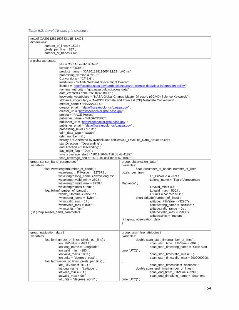
54

Table 6.2: Level-1B data file structure

netcdf OA2011281160543.L1B_LAC { dimensions: number_of_lines = 1502 ; pixels_per_line = 837 ; number_of_bands = 62 ;

// global attributes: :title = "OCIA Level-1B Data" ; :sensor = "OCIA" ; :product_name = "OA2011281160543.L1B_LAC.nc" ; :processing_version = "V1.0" ; :Conventions = "CF-1.6" ; :institution = "NASA Goddard Space Flight Center" ; :license = "http://science.nasa.gov/earth-science/earth-science-data/data-information-policy/"; :naming_authority = "gov.nasa.gsfc.sci.oceandata" ; :date_created = "2016266163258000" ; :keywords_vocabulary = "NASA Global Change Master Directory (GCMD) Science Keywords" ; :stdname_vocabulary = "NetCDF Climate and Forecast (CF) Metadata Convention" ; :creator_name = "NASA/GSFC" ; :creator_email = "[email protected]" ; :creator_url = "http://oceancolor.gsfc.nasa.gov" ; :project = "PACE Project" ; :publisher_name = "NASA/GSFC" ; :publisher_url = "http://oceancolor.gsfc.nasa.gov" ; :publisher_email = "[email protected]" ; :processing_level = "L1B" ; :cdm_data_type = "swath" ; :orbit_number = 0 ; :history = "Generated by avirisbil2oci; cdlfile=OCI_Level-1B_Data_Structure.cdl"; :startDirection = "Descending" ; :endDirection = "Descending" ; :day_night_flag = "Day" ; :time_coverage_start = "2011-10-08T16:05:43.418Z" ; :time_coverage_end = "2011-10-08T16:07:57.108Z" ;

group: sensor_band_parameters { variables: float wavelength(number_of_bands) ; wavelength:_FillValue = -32767.f ; wavelength:long_name = "wavelengths" ; wavelength:valid_min = 350.f ; wavelength:valid_max = 2250.f ; wavelength:units = "nm" ; float fwhm(number_of_bands) ; fwhm:_FillValue = -32767.f ; fwhm:long_name = "fwhm" ; fwhm:valid_min = 0.f ; fwhm:valid_max = 100.f ; fwhm:units = "nm" ; } // group sensor_band_parameters

group: observation_data { variables: float Lt(number_of_bands, number_of_lines, pixels_per_line) ; Lt:_FillValue = -999.f ; Lt:long_name = "Top of Atmosphere Radiance" ; Lt:valid_min = 0.f ; Lt:valid_max = 500.f ; Lt:units = "W m-2 sr-1" ; short altitude(number_of_lines) ; altitude:_FillValue = -32767s ; altitude:long_name = "altitude" ; altitude:valid_range = 0s ; altitude:valid_max = 25000s ; altitude:units = "meters" ; } // group observation_data

}

group: navigation_data { variables: float lon(number_of_lines, pixels_per_line) ; lon:_FillValue = -999.f ; lon:long_name = "Longitude" ; lon:valid_min = -180.f ; lon:valid_max = 180.f ; lon:units = "degrees_east" ; float lat(number_of_lines, pixels_per_line) ; lat:_FillValue = -999.f ; lat:long_name = "Latitude" ; lat:valid_min = -0.f ; lat:valid_max = 90.f ; lat:units = "degrees_north" ;

group: scan_line_attributes { variables: double scan_start_time(number_of_lines) ; scan_start_time:_FillValue = -999. ; scan_start_time:long_name = "Scan start time (UTC)" ; scan_start_time:valid_min = 0. ; scan_start_time:valid_max = 2000000000. ; scan_start_time:units = "seconds" ; double scan_end_time(number_of_lines) ; scan_end_time:_FillValue = -999. ; scan_end_time:long_name = "Scan end time (UTC)" ;

http://science.nasa.gov/earth-science/earth-science-data/data-information-policy/

mailto:[email protected]

http://oceancolor.gsfc.nasa.gov/

http://oceancolor.gsfc.nasa.gov/


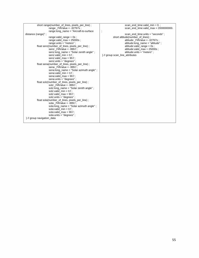
55

short range(number_of_lines, pixels_per_line) ; range:_FillValue = -32767s ; range:long_name = "Aircraft-to-surface distance (range)" ; range:valid_range = 0s ; range:valid_max = 25000s ; range:units = "meters" ; float senz(number_of_lines, pixels_per_line) ; senz:_FillValue = -999.f ; senz:long_name = "Solar zenith angle" ; senz:valid_min = 0.f ; senz:valid_max = 90.f ; senz:units = "degrees" ; float sena(number_of_lines, pixels_per_line) ; sena:_FillValue = -999.f ; sena:long_name = "Solar azimuth angle" ; sena:valid_min = 0.f ; sena:valid_max = 90.f ; sena:units = "degrees" ; float solz(number_of_lines, pixels_per_line) ; solz:_FillValue = -999.f ; solz:long_name = "Solar zenith angle" ; solz:valid_min = 0.f ; solz:valid_max = 90.f ; solz:units = "degrees" ; float sola(number_of_lines, pixels_per_line) ; sola:_FillValue = -999.f ; sola:long_name = "Solar azimuth angle" ; sola:valid_min = 0.f ; sola:valid_max = 90.f ; sola:units = "degrees" ; } // group navigation_data

scan_end_time:valid_min = 0. ; scan_end_time:valid_max = 2000000000. ; scan_end_time:units = "seconds" ; short altitude(number_of_lines) ; altitude:_FillValue = -32767s ; altitude:long_name = "altitude" ; altitude:valid_range = 0s ; altitude:valid_max = 25000s ; altitude:units = "meters" ; } // group scan_line_attributes

56

Chapter 7

PACE Instrument Design Lab Studies – Summary and

Overview on Meeting Science Requirements

Antonio Mannino, NASA Goddard Space Flight Center, Greenbelt, Maryland

Brian Cairns, NASA Goddard Institute for Space Studies, New York, New York

7.

Introduction

The PACE Project conducted a series of Instrument Design Lab (IDL) studies at GSFC, as part of the pre-

Phase A trade studies, to evaluate various instrument concepts to accomplish the mission science

objectives and to meet science requirements while optimizing the PACE instrument capabilities under the

design-to-cost constraints. These IDL studies also addressed many of the science requirement trade

studies that NASA PACE Program Science directed the project to conduct during pre-Phase A

(summarized in Tables 7.1-7.2; see section 7.5 Appendix A for the complete Program Science Trades and

Feasibility Study document). The vast majority of the IDL studies focused on the Ocean Color Instrument

(OCI), since this instrument would be designed to meet and exceed all of the PACE threshold science

requirements. In addition, the project conducted an IDL study for a Multi-Angle Polarimeter (MAP) to

address the Program Scientists’ trade and feasibility recommendations (Table 7.2) and to inform the

project on what could be expected in terms of resources required and performance achieved for an

instrument similar to the MAP described in the PACE SDT report (i.e., CNES-developed Multi-viewing,

Multi-channel, Multi-polarisation Imager or 3MI sensor) in preparation for a formal request for

information (RFI) and a request for proposal (RFP) from industry and other institutions. In addition, the

PACE Program Scientists requested the PACE project to conduct a trade and feasibility study on a high

spatial resolution coastal ocean color sensor (Table 7.3). Therefore, the project conducted a dedicated

coastal camera IDL study and issued an RFI seeking input from industry on potential performance, cost

and size of a coastal camera. The PACE project coordinator for the OCI and coastal camera IDL studies

was Eric Gorman (currently OCI instrument systems engineer). Because the PACE OCI management and

systems engineering team anticipated challenges in meeting the OCI threshold requirements in

conjunction with achieving the goal requirements of 500 m to 250 m or better spatial resolution from a

single instrument, the project decided to separate the higher spatial resolution goal requirements into a

second instrument called the Coastal Camera (CC), which was consistent with the Program Science

Trades and Feasibility Study.

57

Table 7.1: Summary of the Ocean Color Instrument (OCI) trades and feasibility study requested by NASA Program

Science.

Global Ocean Color Sensor (OCI) Design Drivers

Global Coverage 2-day

Lunar Calibration through Earth viewing port that illuminates all detectors at the same time

Spectral range & resolution hyperspectral (5 nm) UV-VIS-NIR

Signal-to-Noise ratio (SNR) consistent with PACE SDT document

Spectral subsampling ~1-2 nm resolution from 655 to 710 nm

Spectral artifacts spectral degradation tracking involving the minimum number of detector

elements possible to minimize striping, cross-talk, and other artifacts in

instrument level data

Driver Consequences

Fore-optics Meeting all design drivers requires a Sea-WiFS-like fore-optics system such that

all ground pixels are observed with the same set of detector elements, which

represents the minimum number of detectors that must be calibrated and tracked

for degradation.

Drawbacks Fast telescope spin rates to enable all science pixels with the same minimum

GSD result in short dwell times on detectors, so increasing spin rate can translate

to decreasing signal or lower SNR

Trade Recommendations

Ground Sample Distance

Baseline 1 km at nadir

(1) evaluate what the highest achievable resolution is that still meets SNR and

other requirements, (2) evaluate what design options/approaches are available to

achieve this resolution at all scan angles

Spectral Range

Baseline resolution of 5 nm

from 350 – 800 nm

evaluate design modifications, risks, and costs for (1) expanding the spectral

range (a) below 350 nm or (b) up to 900 nm, (2) improving resolution to < 5 nm

at either all wavelengths or for specific spectral regions.

SWIR bands Evaluate low-risk instrument modifications required to add the mission threshold

and baseline SWIR measurement requirements onto OCI and determine the

changes in mission risk and changes in total cost to the mission.

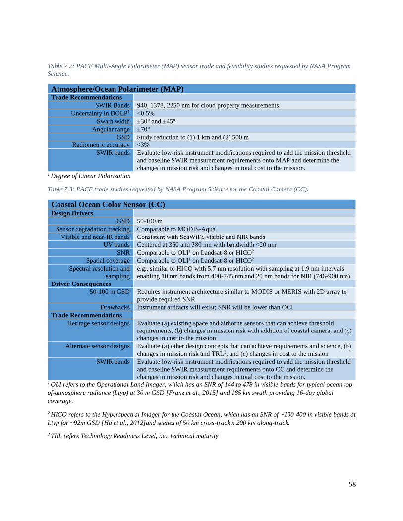
58

Table 7.2: PACE Multi-Angle Polarimeter (MAP) sensor trade and feasibility studies requested by NASA Program

Science.

Atmosphere/Ocean Polarimeter (MAP) Trade Recommendations

SWIR Bands 940, 1378, 2250 nm for cloud property measurements

Uncertainty in DOLP1 <0.5%

Swath width ±30° and ±45°

Angular range ±70°

GSD Study reduction to (1) 1 km and (2) 500 m

Radiometric accuracy <3%


and baseline SWIR measurement requirements onto MAP and determine the

changes in mission risk and changes in total cost to the mission. 1 Degree of Linear Polarization

Table 7.3: PACE trade studies requested by NASA Program Science for the Coastal Camera (CC).

Coastal Ocean Color Sensor (CC) Design Drivers

GSD 50-100 m

Sensor degradation tracking Comparable to MODIS-Aqua

Visible and near-IR bands Consistent with SeaWiFS visible and NIR bands

UV bands Centered at 360 and 380 nm with bandwidth ≤20 nm

SNR Comparable to OLI1 on Landsat-8 or HICO2

Spatial coverage Comparable to OLI1 on Landsat-8 or HICO2

Spectral resolution and

sampling

e.g., similar to HICO with 5.7 nm resolution with sampling at 1.9 nm intervals

enabling 10 nm bands from 400-745 nm and 20 nm bands for NIR (746-900 nm)

Driver Consequences

50-100 m GSD Requires instrument architecture similar to MODIS or MERIS with 2D array to

provide required SNR

Drawbacks Instrument artifacts will exist; SNR will be lower than OCI

Trade Recommendations

Heritage sensor designs Evaluate (a) existing space and airborne sensors that can achieve threshold

requirements, (b) changes in mission risk with addition of coastal camera, and (c)

changes in cost to the mission

Alternate sensor designs Evaluate (a) other design concepts that can achieve requirements and science, (b)

changes in mission risk and TRL3, and (c) changes in cost to the mission


and baseline SWIR measurement requirements onto CC and determine the

changes in mission risk and changes in total cost to the mission. 1 OLI refers to the Operational Land Imager, which has an SNR of 144 to 478 in visible bands for typical ocean top-

of-atmosphere radiance (Ltyp) at 30 m GSD [Franz et al., 2015] and 185 km swath providing 16-day global

coverage.

2 HICO refers to the Hyperspectral Imager for the Coastal Ocean, which has an SNR of ~100-400 in visible bands at

Ltyp for ~92m GSD [Hu et al., 2012]and scenes of 50 km cross-track x 200 km along-track.

3 TRL refers Technology Readiness Level, i.e., technical maturity

59

OCI Study Parameters and Requirements

The project conducted a detailed architecture study on what instrument concepts would be capable of

achieving and exceeding the threshold science requirements attributed to OCI. The team concluded that

three instrument concepts would be worth pursuing in more detail within the GSFC Instrument Design

Lab: HyperSpectral Scanner (HSS), HyperSpectral Pushbroom (HSP), and multi-band scanner (MBS)

(Fig. 7.1).

Figure 7.1. Schematic of the Ocean Color Instrument concepts considered as part of the architecture design study.

Diagram courtesy of Ulrik Gliese, Eric Gorman and Bryan Monosmith.

Over the course of several weeks to several months, a subset of the IDL team worked with the project

to develop a first order optical-mechanical design for each of the three instrument concepts. The maturity

of this preliminary design concept largely determines the level of detail that the IDL team can provide in

their one-week focused study that involves all relevant engineering disciplines (systems, mechanical,

optical, electrical, thermal, radiometry [signal-to-noise determination], detectors, contamination,

reliability, flight software, and cost modeling). The project and OCI systems engineering and instrument

science teams provided the IDL optical and mechanical engineering designers with the starting

parameters for the optical-mechanical design such as platform altitude, instrument ground sample

distance (GSD, spatial resolution), aperture diameter, spectral range, spectral sampling and resolution,

swath width, and field-of-view (FOV). The OCI instrument architecture and science team computed the

aperture diameter based on the PACE OCI signal-to-noise ratio (SNR) science requirements

recommended in the PACE Science Definition Team report [2018]. The GSD for each instrument concept

was based on science requirements and presumed technical feasibility. The IDL pre-work team developed

the following optical-mechanical designs: HSP at 260 m GSD, HSS at 500 m GSD, and MBS at 500 m

GSD. It was well understood that an HSP would be the most capable concept (presumed lowest technical

Ocean Color

Spectrographs

Hyperspectral

Spectrographs

Multiband

Spectrographs

Dispersive Slit

Spectrographs

Interferometric Filter

Spectrographs

Across-track

Slit

Filter

Spectrographs

Along-track

Slit

Multi-Detector

Push Broom

Whisk Broom

Single-Detector

TDI Scanner

Whisk Broom

Multi-Detector

Scanner

Rotating

Multi-Detector

Scanner

Rotating

Single-Detector

TDI Scanner

Multi-Detector

Push Broom

Multi-Detector

Push Broom

Rotating

Multi-Detector

Scanner

Whisk Broom

Multi-Detector

Scanner

Rotating

Single-Detector

TDI Scanner

Whisk Broom

Single-Detector

TDI Scanner

2.2.3

HeritageNone

StudiedNo

HeritageOCM 1 & 2

StudiedCC

HeritageLandsat-5

StudiedNo

HeritageOCTS

MODIS

VIIRSABI

StudiedMBS

HeritageHyperion

MERIS

HICOLandsat-8

OLCI(PRISM –

on aircraft)

StudiedHSP

HeritageNone

StudiedNo

HeritageCZCS

SeaWiFS

(ORCA –lab demo)

StudiedHSS

Heritage(Aerial

Demo by

Aerospace)

StudiedHSW

HeritageLISA

StudiedNo

HeritageNone

StudiedNo

1 2

1.1

1.1.1 1.1.21.1.3

2.2

2.2.1 2.2.2

2.1.1

2.1

2.1.2

2.1.2.12.1.1.32.1.1.1 2.1.1.2

2D

Single-Detector

TDI Scanner

IssuesSimilar to 2.1.1.3 but

more challenging

momentum control.

HeritageNone

StudiedNo

HeritageNone

StudiedNo

IssuesVery complicated

while providing no

benefit over 2.1.1.2 and 2.1.1.3.

IssuesRequires slip ring or

other complicated

harness connection.

2.1.2.2

IssuesRequires slow optics (large f-number) to achieve shallow angles to ensure

good interferometric performance. This results in either increased physical

pixels size or decreased SNR both of which pose performance problems.

IssuesNot hyperspectral and

has more striping than

MBS.

IssuesSimilar to MBS but

more challenging

momentum control.

2.1.2.3

Studied

concepts Hyperspectral

and no stripingSee backup for

details/issues description

60

risk) to achieve the GSD goal requirement while meeting and exceeding the SNR requirements but could

yield image artifacts that would exceed OCI threshold requirements. OCI systems engineering and

management took the lead for the IDL studies from the PACE project perspective. Project science and

OCI instrument science personnel actively participated in each of the IDL studies along with project

management. OCI engineering staff worked closely with the IDL team and in several instances the IDL

team was staffed or otherwise supported by OCI engineers.

For each instrument concept, the IDL team provided to the project the technical resource

requirements (mass, power, data rate, volume, master equipment list (MEL)), parametric instrument cost,

and assessments on performance (SNR, image quality, polarization sensitivity, etc.), technical feasibility,

and risk. Starting from the optical-mechanical design pre-work, the full IDL engineering team developed

a complete first-order design for each of the three OCI concepts over the course of a 5-day study week.

Next, the IDL team and OCI engineers conducted subsequent instrument scaling studies to determine the

technical resource requirements, feasibility, risk, cost, and estimated performance for alternate OCI GSD.

The IDL team studied multiple spatial resolution cases for each concept ranging in GSD from ~250 m to

500 m. Table 7.4 lists the science requirements for each possible sensor concept and GSD case. The color

code in the table denotes whether an instrument concept would be capable of meeting each science

requirement. Technical resource requirements determined from the IDL studies were utilized by the

project to obtain independent cost estimates (Table 7.6) for the various instrument concepts. It should be

noted that GSFC had been studying the HSS concept since 2001 under the name Ocean Radiometer for

Carbon Assessment (ORCA) including two Instrument Incubator Program-funded projects and several

IDL studies over the course of about 10 years [McClain et al., 2012]. Thus, this concept was by far the

best understood.

The HSS concept draws its heritage from the earliest ocean color satellite sensors, the Coastal Zone

Color Scanner (CZCS) and the Sea-Viewing Wide Field-of-View Sensor (SeaWiFS). The front-end optics

of the HSS concept is composed of a rotating telescope similar to SeaWiFS. This rotating telescope

sweeps the slit across the flight track onto effectively a single detector time-delay integration (TDI)

system. This is the concept that the project ultimately selected as the most capable for meeting the

mission science requirements.

The MBS concept possesses similarities in design to VIIRS, SeaWiFS, and MODIS. Like VIIRS and

SeaWiFS, the front-end optics of the MBS concept is composed of a rotating telescope assembly.

Multiple detectors are employed to accomplish measurements for 39 spectral bands between 350 nm to

2250 nm band centers. This approach is similar to MODIS and VIIRS, which enables the heritage sensors

to collect observations at 250 m and 375 m GSD, respectively.

The HSP concept is a pushbroom sensor composed of multiple cameras to achieve the desired cross-

track field-of-view. Heritage pushbroom instruments include MERIS, Hyperion, OLI, HICO, and OLCI.

The 260 m GSD concept was comprised of 6 cameras each with a 28 mm pupil diameter, which was

oversized due to an erroneous calculation by an OCI team member during the optical design development.

This resulted in too much light entering the focal planes of each camera requiring the incoming signal to

be attenuated by a factor of 2 with neutral density filters (implemented in the design to prevent saturation

of the detectors). A more appropriate pupil diameter would have yielded a smaller instrument concept.

The HSP 500 m version was a 5-camera system with a properly sized 12 mm pupil diameter.

The technical resource requirements and SNR performance results from the IDL study illustrate

significant differences among the three sensor concepts. MBS concepts are by far the largest in mass and

volume and HSS was generally smaller and lighter than the other two concepts except for the HSP 500 m

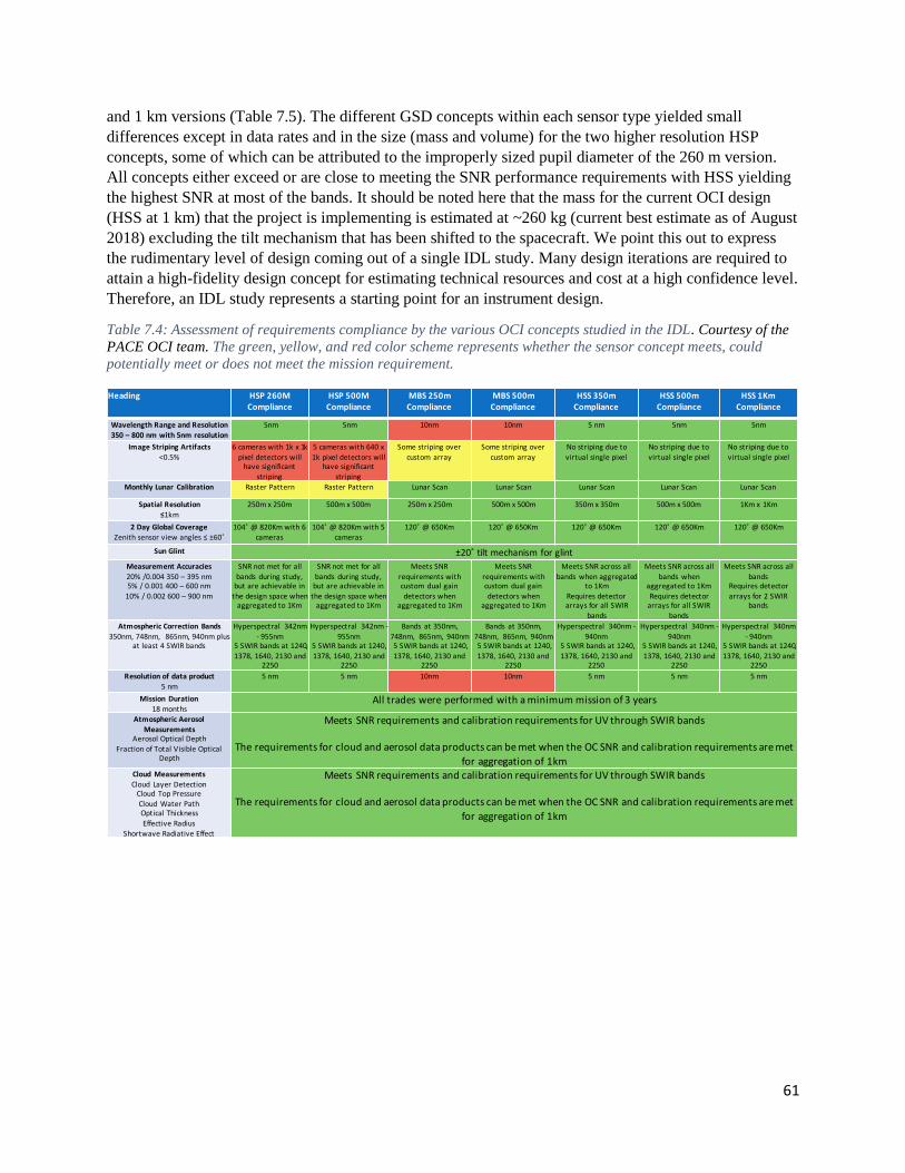
61

and 1 km versions (Table 7.5). The different GSD concepts within each sensor type yielded small

differences except in data rates and in the size (mass and volume) for the two higher resolution HSP

concepts, some of which can be attributed to the improperly sized pupil diameter of the 260 m version.

All concepts either exceed or are close to meeting the SNR performance requirements with HSS yielding

the highest SNR at most of the bands. It should be noted here that the mass for the current OCI design

(HSS at 1 km) that the project is implementing is estimated at ~260 kg (current best estimate as of August

2018) excluding the tilt mechanism that has been shifted to the spacecraft. We point this out to express

the rudimentary level of design coming out of a single IDL study. Many design iterations are required to

attain a high-fidelity design concept for estimating technical resources and cost at a high confidence level.

Therefore, an IDL study represents a starting point for an instrument design.

Table 7.4: Assessment of requirements compliance by the various OCI concepts studied in the IDL. Courtesy of the

PACE OCI team. The green, yellow, and red color scheme represents whether the sensor concept meets, could

potentially meet or does not meet the mission requirement.

Heading HSP260MCompliance

HSP500MCompliance

MBS250mCompliance

MBS500mCompliance

HSS350mCompliance

HSS500mCompliance

HSS1KmCompliance

WavelengthRangeandResolution

350– 800nmwith5nmresolution

5nm 5nm 10nm 10nm 5nm 5nm 5nm

ImageStripingArtifacts

<0.5%

6cameraswith1kx1k

pixeldetectorswillhavesignificant

striping

5cameraswith640x

1kpixeldetectorswillhavesignificant

striping

Somestripingover

customarray

Somestripingover

customarray

Nostripingdueto

virtualsinglepixel

Nostripingdueto

virtualsinglepixel

Nostripingdueto

virtualsinglepixel

MonthlyLunarCalibration RasterPattern RasterPattern LunarScan LunarScan LunarScan LunarScan LunarScan

SpatialResolution

≤1km

250mx250m 500mx500m 250mx250m 500mx500m 350mx350m 500mx500m 1Kmx1Km

2DayGlobalCoverage

Zenithsensorviewangles≤±60˚

104˚@820Kmwith6

cameras

104˚@820Kmwith5

cameras

120˚@650Km 120˚@650Km 120˚@650Km 120˚@650Km 120˚@650Km

SunGlint ±20˚tiltmechanismforglint

MeasurementAccuracies

20%/0.004350– 395nm5%/0.001400– 600nm

10%/0.002600– 900nm

SNRnotmetforall

bandsduringstudy,butareachievablein

thedesignspacewhenaggregatedto1Km

SNRnotmetforall

bandsduringstudy,butareachievablein

thedesignspacewhenaggregatedto1Km

MeetsSNR

requirementswithcustomdualgain

detectorswhenaggregatedto1Km

MeetsSNR

requirementswithcustomdualgain

detectorswhenaggregatedto1Km

MeetsSNRacrossall

bands whenaggregatedto1Km

RequiresdetectorarraysforallSWIR

bands

MeetsSNRacrossall

bandswhenaggregatedto1Km

RequiresdetectorarraysforallSWIR

bands

MeetsSNRacrossall

bandsRequiresdetector

arraysfor2SWIRbands

AtmosphericCorrectionBands

350nm,748nm,865nm,940nmplusatleast4SWIRbands

Hyperspectral342nm

- 955nm5SWIRbandsat1240,

1378,1640,2130and2250

Hyperspectral342nm-

955nm5SWIRbandsat1240,

1378,1640,2130and2250

Bandsat350nm,

748nm,865nm,940nm5SWIRbandsat1240,

1378,1640,2130and2250

Bandsat350nm,

748nm,865nm,940nm5SWIRbandsat1240,

1378,1640,2130and2250

Hyperspectral340nm-


1378,1640,2130and2250

Hyperspectral340nm-


1378,1640,2130and2250

Hyperspectral340nm

- 940nm5SWIRbandsat1240,

1378,1640,2130and2250

Resolutionofdataproduct

5nm

5nm 5nm 10nm 10nm 5nm 5nm 5nm

MissionDuration

18monthsAlltradeswereperformedwithaminimummissionof3years

AtmosphericAerosol

MeasurementsAerosolOpticalDepth

FractionofTotalVisibleOpticalDepth

MeetsSNRrequirementsand calibrationrequirementsforUVthroughSWIRbands

TherequirementsforcloudandaerosoldataproductscanbemetwhentheOCSNRandcalibrationrequirementsaremet

foraggregationof1kmCloudMeasurements

CloudLayerDetectionCloudTopPressure

CloudWaterPathOpticalThickness

EffectiveRadius

ShortwaveRadiativeEffect

MeetsSNRrequirementsand calibrationrequirementsforUVthroughSWIRbands

TherequirementsforcloudandaerosoldataproductscanbemetwhentheOCSNRandcalibrationrequirementsaremet

foraggregationof1km

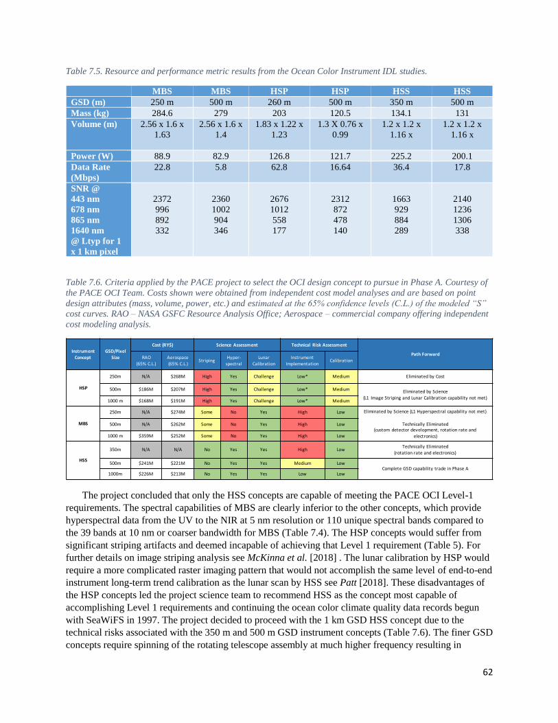
62

Table 7.5. Resource and performance metric results from the Ocean Color Instrument IDL studies.

MBS MBS HSP HSP HSS HSS

GSD (m) 250 m 500 m 260 m 500 m 350 m 500 m

Mass (kg) 284.6 279 203 120.5 134.1 131

Volume (m) 2.56 x 1.6 x

1.63

2.56 x 1.6 x

1.4

1.83 x 1.22 x

1.23

1.3 X 0.76 x

0.99

1.2 x 1.2 x

1.16 x

1.2 x 1.2 x

1.16 x

Power (W) 88.9 82.9 126.8 121.7 225.2 200.1

Data Rate

(Mbps)

22.8 5.8 62.8 16.64 36.4 17.8

SNR @

443 nm

678 nm

865 nm

1640 nm

@ Ltyp for 1

x 1 km pixel

2372

996

892

332

2360

1002

904

346

2676

1012

558

177

2312

872

478

140

1663

929

884

289

2140

1236

1306

338

Table 7.6. Criteria applied by the PACE project to select the OCI design concept to pursue in Phase A. Courtesy of

the PACE OCI Team. Costs shown were obtained from independent cost model analyses and are based on point

design attributes (mass, volume, power, etc.) and estimated at the 65% confidence levels (C.L.) of the modeled “S”

cost curves. RAO – NASA GSFC Resource Analysis Office; Aerospace – commercial company offering independent

cost modeling analysis.

The project concluded that only the HSS concepts are capable of meeting the PACE OCI Level-1

requirements. The spectral capabilities of MBS are clearly inferior to the other concepts, which provide

hyperspectral data from the UV to the NIR at 5 nm resolution or 110 unique spectral bands compared to

the 39 bands at 10 nm or coarser bandwidth for MBS (Table 7.4). The HSP concepts would suffer from

significant striping artifacts and deemed incapable of achieving that Level 1 requirement (Table 5). For

further details on image striping analysis see McKinna et al. [2018] . The lunar calibration by HSP would

require a more complicated raster imaging pattern that would not accomplish the same level of end-to-end

instrument long-term trend calibration as the lunar scan by HSS see Patt [2018]. These disadvantages of

the HSP concepts led the project science team to recommend HSS as the concept most capable of

accomplishing Level 1 requirements and continuing the ocean color climate quality data records begun

with SeaWiFS in 1997. The project decided to proceed with the 1 km GSD HSS concept due to the

technical risks associated with the 350 m and 500 m GSD instrument concepts (Table 7.6). The finer GSD

concepts require spinning of the rotating telescope assembly at much higher frequency resulting in

Instrument

Concept

GSD/Pixel

Size

Cost(RY$) ScienceAssessment TechnicalRiskAssessment

Path ForwardRAO

(65%C.L.)

Aerospace

(65% C.L.)Striping

Hyper-

spectral

Lunar

Calibration

Instrument

ImplementationCalibration

HSP

250m N/A $268M High Yes Challenge Low* Medium EliminatedbyCost

500m $186M $207M High Yes Challenge Low* Medium Eliminated byScience

(L1ImageStripingandLunarCalibrationcapabilitynotmet)1000m $168M $191M High Yes Challenge Low* Medium

MBS

250m N/A $274M Some No Yes High Low EliminatedbyScience(L1Hyperspectralcapabilitynotmet)

TechnicallyEliminated(customdetectordevelopment,rotation rateand

electronics)

500m N/A $262M Some No Yes High Low

1000m $359M $252M Some No Yes High Low

HSS

350m N/A N/A No Yes Yes High LowTechnicallyEliminated

(rotation rateandelectronics)

500m $241M $221M No Yes Yes Medium LowCompleteGSDcapabilitytradeinPhaseA

1000m $226M $213M No Yes Yes Low Low

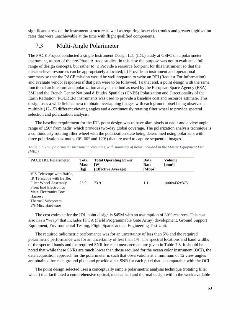
63

significant stress on the instrument structure as well as requiring faster electronics and greater digitization

rates that were unachievable at the time with flight qualified components.

Multi-Angle Polarimeter

The PACE Project conducted a single Instrument Design Lab (IDL) study at GSFC on a polarimeter

instrument, as part of the pre-Phase A trade studies. In this case the purpose was not to evaluate a full

range of design concepts, but rather to: i) Provide a resource footprint for this instrument so that the

mission-level resources can be appropriately allocated; ii) Provide an instrument and operational

summary so that the PACE mission would be well prepared to write an RFI (Request For Information)

and evaluate vendor responses if that path were to be followed. To that end, a point design with the same

functional architecture and polarization analysis method as used by the European Space Agency (ESA)

3MI and the French Centre National d’Etudes Spatiales (CNES) Polarization and Directionality of the

Earth Radiation (POLDER) instruments was used to provide a baseline cost and resource estimate. This

design uses a wide field camera to obtain overlapping images with each ground pixel being observed at

multiple (12-15) different viewing angles and a continuously rotating filter wheel to provide spectral

selection and polarization analysis.

The baseline requirement for the IDL point design was to have 4km pixels at nadir and a view angle

range of ±50° from nadir, which provides two-day global coverage. The polarization analysis technique is

a continuously rotating filter wheel with the polarization state being determined using polarizers with

three polarization azimuths (0°, 60° and 120°) that are used to capture sequential images.

Table 7.7. IDL polarimeter instrument resources, with summary of items included in the Master Equipment List

(MEL).

PACE IDL Polarimeter Total

Mass

[kg]

Total Operating Power

[W]

(Effective Average)

Data

Rate

[Mbps]

Volume

[mm3]

VIS Telescope with Baffle,

IR Telescope with Baffle,

Filter Wheel Assembly

Front End Electronics

Main Electronics Box

Harness

Thermal Subsystem

5% Misc Hardware

25.9

73.9

1.1

1000x432x375

The cost estimate for the IDL point design is $45M with an assumption of 30% reserves. This cost

also has a “wrap” that includes FPGA (Field Programmable Gate Array) development, Ground Support

Equipment, Environmental Testing, Flight Spares and an Engineering Test Unit.

The required radiometric performance was for an uncertainty of less than 5% and the required

polarimetric performance was for an uncertainty of less than 1%. The spectral locations and band widths

of the spectral bands and the required SNR for each measurement are given in Table 7.8. It should be

noted that while these SNRs are much lower than those required for the ocean color instrument (OCI), the

data acquisition approach for the polarimeter is such that observations at a minimum of 12 view angles

are obtained for each ground pixel and provide a net SNR for each pixel that is comparable with the OCI.

The point design selected uses a conceptually simple polarimetric analysis technique (rotating filter

wheel) that facilitated a comprehensive optical, mechanical and thermal design within the week available

64

for the study. The wide field of view camera implementation with two-day global coverage is a good

match to the required global coverage for the OCI sensor.

Table 7.8. Specification of spectral bands and signal to noise ratio (SNR) for the IDL polarimeter design. Bands

with a * include polarization measurements.

Center

Wavelength

(nm)

Band Width

(nm)

SNR

412* 20 100

443* 20 100

490* 20 100

555* 20 100

670* 20 100

763 10 100

765 40 100

865* 39 100

910 20 70

1378* 35 50

1610* 60 100

2130* 75 100

The sequential polarization analysis technique provides no guaranteed polarimetric accuracy over

heterogeneous scenes, since changes in total radiance between sequential measurements can be aliased

into apparent changes in polarization. While this would not be an issue for clear scenes over ocean, it

would present challenges in analyzing the data over land.

The point design based on a 3MI/POLDER type sensor that the IDL analyzed provided useful

information on likely resource requirements. It also allowed the feasibility of meeting performance

requirements with a simple, compact sensor to be assessed and helped to define the scope of the

information that would be required in an RFI/RFP if the project were to procure a polarimeter.

Coastal Camera

The PACE SDT Report identified a scientific goal for multi- to hyperspectral ocean color observations at

a ground sample distance (GSD) of 250 m or better and identified advantages of similar GSD capability

for cloud and aerosol studies. PACE Program Scientists recommended the project study the feasibility of

a 50-100 m spatial resolution Coastal Camera for ocean color observations at the land-water interface and

for detection of events such as oil spills and harmful algal blooms (see section 7.5 Appendix A). In

coastal ecosystems, physical processes regulate the spatial-temporal dynamics of biological and

biogeochemical processes and constituent distributions. High spatial resolution capability is necessary to

resolve the spatial variability of these processes and constituents. A sensor on the order of 100 m GSD on

PACE would spatially resolve the biogeochemical properties and their responses to physical processes

within coastal ocean, estuarine and inland waters including phytoplankton blooms, water quality, and

gradients of materials across coastal plumes, and further our understanding of the role of continental

margins in carbon export. Hence as part of the pre-phase A trade studies, the project explored concepts

65

for a high spatial resolution coastal camera through an RFI (see section 7.6 Appendix B) and an IDL

study. The information obtained from the RFI is proprietary and thus not included in this document. The

aim for the CC IDL study was to determine whether a low-cost (~$10M) do-no-harm instrument would be

feasible for accomplishing PACE science goals. The IDL Coastal Camera uses a simple refractive optical

design (a single pushbroom camera) and a butcher-block filter assembly to image 12 bands onto a single

off the shelf detector. An additional two spectral bands could be added with little to no impact on the

design and cost. Several innovative design ideas allowed for incorporation of advanced features such as

the cross-track rotation mechanism (leadscrew stepper motor) and the solar calibration capability at the 0

tilt position using a stationary Spectralon reflective diffuser; science observations would be conducted at

the 20 tilt positions. In addition, the estimated SNR performance for the specified OCI Ltyp values and

bandwidths are in-line with OCI requirements (Table 7.9). In summary, the IDL study produced a

complete and technically viable coastal camera concept that could provide scientific value to PACE.

However, the in-house and independent cost estimates exceeded the available project resources. Thus, the

project decided that it could not pursue either an in-house or procured coastal camera.

Table 7.9. Specifications, resource and performance metric results from the Coastal Camera IDL studies.

Coastal Camera

GSD (m) 100 m

Spectral Band Centers

and Bandwidth (nm)

Band Bandwidth

360 15

412 10

443 10

490 10

510 10

555 10

617 10

665 10

678 10

710 10

748 10

865 15

FOV

cross-track 12.7 15 with rotation mechanism

Swath 160 km

Sun glint 20 tilt

with mechanism

Solar Cal Daily stationary Spectralon diffuser

Lunar Cal Monthly

Mass (kg) 23.7

Volume (m) 0.763 m x 0.61 m diameter

MEB: 0.018 x 0.024 x 0.015m

Power (W) 42.9

Data Rate (Mbps) 15.2

SNR @

443 nm

555 nm

678 nm

865 nm

@ Ltyp for 100 x 100 m

pixel

1667

1237

798

533

66

Appendix A: PACE Program Science Trades and Feasibility

Study Document (Version 5 – May 8, 2015)

7.5.1. Trade Studies on PACE.

The PACE mission is intended to serve multiple science disciplines, including supporting observations

for ocean, aerosol, and cloud investigations. A variety of configurations can be envisioned for the mission

payload, but the funding framework is ‘design to cost’. To optimize science returns from the mission, it is

desired that focused studies be conducted regarding potential measurement trades/feasibility. This

document outlines three sets of specific desired trade/feasibility studies, with a requirement that due

diligence is documented regarding the evaluation of each. The framework assumed here is that of a

‘modular’ instrument configuration for the mission sensors (in the sense that a combination of more than

two separate instruments could be considered), with the desired studies organized with respect to a

module. It is recommended that these studies follow a series of milestones, in the order: (1) evaluate the

technical feasibility of the various options (and if it is not technically feasible, document why), (2) report

out, (3) provide a cost estimate on the technically feasible options, and (4) conduct the cost delta

evaluation relative to the baseline configuration.

Module 1: Global Ocean Color Sensor (GOCS)

Design drivers – (1) Lunar calibration through Earth viewing port that illuminates all detectors at the

same time, (2) Spectral system degradation tracking involving the minimum number of ‘detector

elements’ possible to minimize striping, cross-talk, and other artifacts in instrument level data, (2)

hyperspectral (5 nm) UV-VIS-NIR resolution, (4) SNR’s consistent with SDT document, (5) 2-day global

coverage, (6) pectral subsampling at ~1-2 nm resolution from 655 to 710 nm (to enable refined

characterization of the chlorophyll fluorescence spectrum).

Driver consequences – Meeting the above design drivers (particularly 1 & 2) with a demonstrated

approach requires that the GOCS falls into the SeaWiFS-like category of sensor types, in the sense of

fore-optics. In other words, all ground pixels are observed with the same set of detector elements, which

represents the minimum number of detectors that must be calibrated and tracked for degradation.

Drawbacks of this approach are that telescope spin rates are fast and all science pixels have the same

minimum ground dimension. Rapid spin rates equate to short dwell times on detectors, so increasing spin

rate can translate to decreasing signal or lower SNR, which can jeopardize key science aspects of the

mission, including continuity of fluorescence retrievals.

Trade/feasibility Recommendations –

(1) If the baseline ground resolution for GOCS is 1 km at nadir, evaluate what the highest achievable

resolution is that still meets SNR (and other) requirements. This evaluation needs to consider (a)

modifications to the baseline design, such as increasing detector-detector integration to increase SNR, (b)

changes in mission risk due to higher resolution (e.g., sensor lifetime, increased complexity/optical or

electrical components), and (c) changes in cost due to increased data download/handling, design and

construction, mass, etc.

67

(2) For a given design for the spatial resolution identified in (1) above, evaluate what design

options/approaches are available to achieve this resolution at all scan angles. This evaluation needs to

consider changes in design, risk, and cost (as above),

(3) If the baseline UV-VIS-NIR resolution for GOCS is 5 nm from 350 – 800 nm, evaluate design

modifications, risks, and costs for (a) expanding this range below 350 nm or to 900 nm and (b) improving

resolution to < 5 nm at either all wavelengths or for specific spectral regions.

Module 2: Coastal Ocean Color Sensor (COCS)

Design drivers – (1) Ocean color measurements near land-ocean interfaces and for specific events (e.g.,

oil spills, cruise support) at 50 – 100 meter resolution, (2) Sensor degradation tracking comparable to

MODIS Aqua, (3) ≤20 nm bandwidth spectral measurement bands with center wavelengths at 360 and

380 nm and additional bands consistent with the SeaWiFS at visible and NIR wavelengths, (4) SNR’s and

spatial coverage comparable to OLI on Landsat-8 or HICO. With respect to spectral resolution, one

example of an overall approach that might be considered is something similar to HICO (As an example,

HICO provided data at 5.7 nm spectral resolution, with spectral data collected at 1.9 nm resolution. To

increase the signal to noise ratio, three bands were combined on the detector to produce wavelength

centers 5.7 nm apart. A smoothing filter (Gaussian) was then applied to the uncalibrated spectral data to

fix etaloning at the longer wavelengths. The size of the filter is 1Hi0 nm for the shorter wavelengths (400

- 745 nm) and 20 nm for the longer wavelengths (746 - 900 nm). Thus the data are 10 (or 20) nm width

data centered on 5.7 nm wavelength centers.)

Driver consequences – Meeting the above design drivers (particularly 1) with a demonstrated approach

requires that the COCS falls into the MODIS-like or MERIS-like category of sensor types, in the sense

that (a) 2-dimensional detector array(s) is (are) required for sufficient dwell time to achieve appropriate

SNR’s. Drawbacks of these approaches are that instrument artifacts are likely to exist in, even up to Level

3, retrieved products and SNR’s will be lower than for the GOCS. A SeaWiFS-type sensor will not work

for this module.


(1) Evaluate existing sensor designs (space or aircraft heritage) that can achieve instrument/science

requirements for COCS. This evaluation needs to consider (a) simplifications to heritage designs that

reduce cost or complexity while achieving threshold requirements, (b) changes in mission risk associated

with Module 2 and its addition to the mission payload, and (c) changes in cost due to increased data

download/handling, design & construction, mass, etc.

(2) Evaluate alternative sensor designs (i.e., different than heritage sensors) that can achieve

instrument/science requirements for COCS. This evaluation needs to consider (a) minimum sensor design

requirements to achieve science threshold requirements, (b) changes in mission risk due to addition of the

instrument to the mission payload and TRL, and (c) changes in cost due to increased data

download/handling, design & construction, mass, etc.

68

Module 3: Atmosphere/Ocean Polarimeter (AOP)

Design drivers –

Driver consequences –


Recommended Cost Trade Studies

(1) Inclusion / Addition of bands at 940, 1378, 2250 for cloud property measurements

(2) Reduction of the uncertainty in DOLP to 0.5%

(3) Increase swath width to ±30° and ±45°

(4) Increase the number of measurement angles to 50 and 100

(5) Increase in angular range to ±70°

(6) Reduce pixel size to 1 km and 500 m

(7) Improve radiometric accuracy to 3%

Additional Trade/Feasibility Studies

Mission observations at specific short-wave infrared bands (SWIR) are desirable for multiple coastal and

atmospheric science applications. However, the platform instrument module used to achieve these

measurements is flexible. The ocean science application for the SWIR data is for improved atmospheric

corrections in highly turbid (e.g., coastal, estuarine) waters, where water leaving radiances in the NIR are

non-negligible. Accordingly, inclusion of the SWIR bands on the COCS, rather than GOCS, may be

preferable. A disadvantage of integrating the SWIR bands into the COCS instrument is its likely narrower

swath width and the GOCS instrument, which may diminish atmospheric science returns. Alternatively, it

may be advantageous to make the SWIR measurements from the AOP. Given the ‘design to cost’

framework for the PACE mission, it is desired that trade/feasibility studies be conducted to evaluate these

three SWIR integration options (i.e., as part of the GOCS, COCS, and AOP modules). These evaluations

allow informed decisions regarding the SWIR measurements for various mission scenarios involving one,

two, or three modules.

Design drivers – Threshold and baseline SWIR measurements with bandwidths, band centers, and SNR

requirements as defined by the mission SDT.


(1) Evaluate instrument designs modifications necessary to include the threshold and baseline SWIR

measurement requirements into the COCS module. This evaluation needs to consider (a) low-risk

instrument design options to achieve requirements, (b) changes in mission risk due to addition of the

SWIR measurement capability, and (c) changes in cost due to increased data download/handling, design

& construction, mass, etc.


measurement requirements into the GOCS module. This evaluation needs to consider (a) low-risk




69


measurement requirements into the AOP module. This evaluation needs to consider (a) low-risk




70

Appendix B: Coastal Camera Request for Information (RFI)

REQUEST FOR INFORMATION (RFI)

Pre-Aerosol, Clouds and Oceans Ecosystem (PACE) mission

THIS IS *NOT* A REQUEST FOR PROPOSAL OR INVITATION TO BID NOTICE.

The Pre-Aerosol, Clouds and Oceans Ecosystem (PACE) Project is considering the purchase of multi-

band high spatial resolution camera to complement its primary ocean color instrument. The PACE

mission is primarily being conducted to collect global measurements of ocean color. These measurements

will extend contemporary data records of ocean ecological and marine biogeochemical parameters. The

multi-band high spatial resolution camera will collect additional data at high spatial resolution when the

PACE observatory is in sight of coastal regions. This data will be combined with hyperspectral data from

the primary ocean color instrument with lower spatial resolution.

PACE will enable advanced research on:

• Plankton Stocks – Distinguish living phytoplankton from other optically-active water column

constituents, such as re-suspended sediments and dissolved carbon;

• Plankton Diversity – Identify phytoplankton community structure;

• Ocean Carbon – Assess changes in carbon stocks, primary production, net community

production, and carbon export to the deep sea;

• Human Impacts – Evaluate changes in land-ocean interactions and water quality;

• Forecasting Futures – Resolve mechanistic linkages between biology and environmental physical

forcings to support of process-based predictive modeling.

The purpose of this RFI is to identify potential interest in providing a multi-band high spatial resolution

camera for the PACE Project. This is for information and planning purposes and to allow industry the

opportunity to verify reasonableness and feasibility of the requirements and to promote competition.

While our intent may be to team with industrial partner(s), we are not bound by this RFI to do so. This is

not a Request for Proposal, nor a Request for Quotation, nor an Invitation to Bid. Therefore, this RFI is

not to be construed as a commitment by the Government to enter into a contract nor will the Government

pay for information provided in response to this RFI.

The desired characteristics for the multi-band high spatial resolution camera are the following:

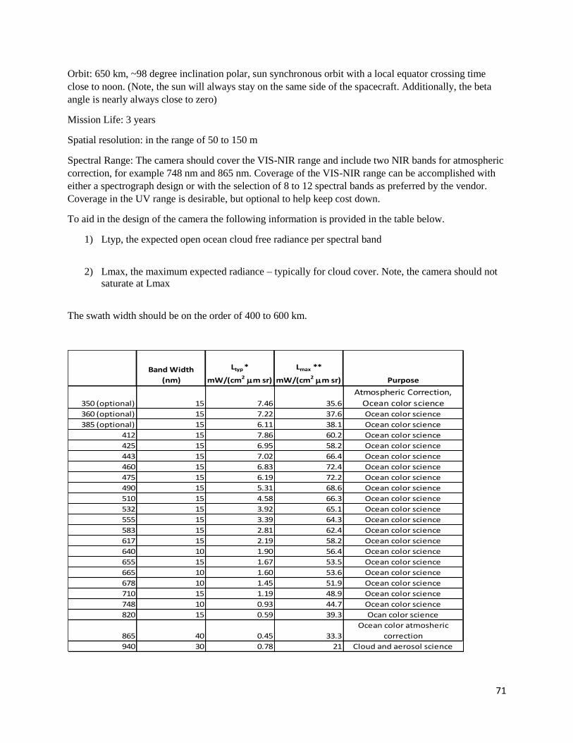
71

Orbit: 650 km, ~98 degree inclination polar, sun synchronous orbit with a local equator crossing time

close to noon. (Note, the sun will always stay on the same side of the spacecraft. Additionally, the beta

angle is nearly always close to zero)

Mission Life: 3 years

Spatial resolution: in the range of 50 to 150 m

Spectral Range: The camera should cover the VIS-NIR range and include two NIR bands for atmospheric

correction, for example 748 nm and 865 nm. Coverage of the VIS-NIR range can be accomplished with

either a spectrograph design or with the selection of 8 to 12 spectral bands as preferred by the vendor.

Coverage in the UV range is desirable, but optional to help keep cost down.

To aid in the design of the camera the following information is provided in the table below.

1) Ltyp, the expected open ocean cloud free radiance per spectral band

2) Lmax, the maximum expected radiance – typically for cloud cover. Note, the camera should not

saturate at Lmax

The swath width should be on the order of 400 to 600 km.

Band Width

(nm)

Ltyp *

mW/(cm2 mm sr)

Lmax **

mW/(cm2 mm sr) Purpose

350 (optional) 15 7.46 35.6

Atmospheric Correction,

Ocean color science360 (optional) 15 7.22 37.6 Ocean color science

385 (optional) 15 6.11 38.1 Ocean color science

412 15 7.86 60.2 Ocean color science

















820 15 0.59 39.3 Ocan color science

865 40 0.45 33.3

Ocean color atmosheric

correction

940 30 0.78 21 Cloud and aerosol science

72

This RFI is to solicit specific capability information from industry and promote competition. For planning

purposes, we are requesting that the responses to this RFI include the following information:

1) A brief description of the technical capabilities, key interfaces, and heritage of the camera.

2) Provide the expected Signal to Noise Ratios that can be achieved with the camera.

3) The approximate mass, power and volume requirements for a single camera. How do these

requirements change with the addition of a second and/or third camera?

4) A brief description of company capabilities, applicable facilities, and experience designing and

building cameras.

5) Notional schedule for instrument implementation through delivery to the project. The vendor

should assume an authority to proceed data of April 2017.

6) The approximate cost of a single camera design and the cost of adding a second and/or possibly a

third camera. Costs should be in real year dollars.

7) Description of key technical, schedule, and price drivers and options to mitigate risks and/or

reduce schedule.

To consolidate our planning, responses from industry are requested by Friday, August 14, 2015, in the

form of written and illustrated concepts, estimates for development costs and schedule, assumptions used

for cost and schedule estimates including interface and design assumptions, and descriptions of

capabilities. Responses can be submitted via email. The subject line of the submission should be "RFI for

Multi-band Camera,” and attachments should be in Microsoft WORD, POWERPOINT, or PDF format.

The email text must give a point-of-contact and provide his/her name, address, telephone/fax numbers,

and email address. The information is requested for planning purposes only, subject to FAR Clause

52.215-3, entitled "Solicitation for Information for Planning Purposes."

It is not NASA's intent to publicly disclose vendor proprietary information obtained during this

solicitation. To the full extent that it is protected pursuant to the Freedom of Information Act and other

laws and regulations, information identified by a respondent as "Proprietary or Confidential" will be kept

confidential.

It is emphasized that this RFI is for planning and information purposes only and is NOT to be construed

as a commitment by the Government to enter into a contractual agreement, nor will the Government pay

for information solicited.

No solicitation exists; therefore, do not request a copy of the solicitation. If a solicitation is released, it

will be synopsized in FedBizOpps and on the NASA Acquisition Internet Service. It is the potential

offeror’s responsibility to monitor these sites for the release of any solicitation or synopsis.

Technical questions should be directed to: Leslie Hartz at [email protected] or Eric Gorman at

[email protected]. Procurement related questions should be directed to: Ayana Briscoe at

[email protected]

Interested offerors shall address the requirements of this RFI in written format as described in the

previous paragraphs by electronic mail to: Leslie Hartz at [email protected], no later than 5:00

PM EST on Friday, August 14, 2015.

An ombudsman has been appointed -- See NASA Specific Note "B".





73

The solicitation and any documents related to this procurement will be available over the Internet. These

documents will be in Microsoft Office 97 format and will reside on a World Wide Web (WWW) server,

which may be accessed using a WWW browser application. The Internet site, or URL, for the

NASA/GSFC Business Opportunities home page is http://prod.nais.nasa.gov/cgi-

bin/eps/bizops.cgi?gr=C&pin=51. It is the offeror's responsibility to monitor the Internet site for the

release of the solicitation and amendments (if any). Potential offerors will be responsible for downloading

their own copy of the solicitation and amendments, if any. Any referenced notes may be viewed at the

following URLs linked below.

http://prod.nais.nasa.gov/cgi-bin/eps/bizops.cgi?gr=C&pin=51

http://prod.nais.nasa.gov/cgi-bin/eps/bizops.cgi?gr=C&pin=51

74

Chapter 8

Case for the Addition of a Coastal Ocean Color Imager

(COCI) to PACE

Antonio Mannino, NASA Goddard Space Flight Center, Greenbelt, Maryland7

Susanne E. Craig, GESTAR/Universities Space Research Association, Columbia, Maryland

Nima Pahlevan, Science Systems and Applications Inc, Lanham, MD

8.

Executive Summary

This chapter describes the scientific justifications for the addition of a hyperspectral coastal ocean color

imager (COCI) to the PACE mission. COCI was specifically designed to image small-scale to mesoscale

processes in the coastal ocean, estuarine, and inland waters. This pushbroom sensor has a nominal ground

sample distance of 100 m, and spectral characteristics equivalent to the PACE Ocean Color Instrument

(OCI). The information acquired from such a sensor is highly complementary to ocean color and

atmospheric measurements from OCI and polarimeters. Principally, COCI would substantially enhance

the capabilities of PACE to reveal ecological and biogeochemical processes in these important, but

vulnerable, waters. Many individuals contributed to defining the PACE-relevant science and requirements

associated with COCI (see Tables 8.2 and 8.3 for a complete list).

Introduction

The NASA Climate-Centric Architecture document included an objective for the PACE ocean color

instrument to quantify water quality in coastal regions with “new, high quality information on the

biogeochemical properties of coastal waters and their implications for ecosystem and human health”

[NASA, 2010, p. 20]. The PACE Science Definition Team (SDT) Report [PACE Science Definition Team,

2018] identified a scientific goal for multi- to hyperspectral ocean color observations at a ground sample

distance (GSD) of 250 m and identified advantages of similar GSD capability for cloud and aerosol

studies. The Report described several benefits that would result if PACE met these goal requirements

[NASA, 2010, p. xvii]:

• “Increase the area of inland waters that can be studied using remote

sensing, including increased coverage of the Great Lakes and a large

number of smaller water bodies

• Increase temporal resolution by reducing interference from clouds

• Improve satellite product validation in coastal areas where large spatial

gradients in observable variables are expected

7 Cite as: Mannino, A., S. E. Craig, and N. Pahlevan (2018), Case for the Addition of a Coastal Ocean Color Imager (COCI) to

PACE, in PACE Technical Report Series, Volume 5: Mission Formulation Studies (NASA/TM-2018 – 2018-219027/ Vol. 5),

edited by I. Cetinić, C. R. McClain and P. J. Werdell, NASA Goddard Space Flight Space Center Greenbelt, MD.

75

• Increase the use of satellite ocean color observations in coastal research

and management applications globally

• Develop and implement applications to advance assessments of critical

ocean ecosystem services [that] affect human health and welfare”

Under Design-to-Cost (DTC) constraints, the PACE Project determined that it could not achieve both

the threshold requirements and the high spatial resolution goal recommended by the PACE SDT with a

single sensor. The Program Scientists requested the Project explore the feasibility of including a high

spatial resolution instrument for coastal environments (i.e., coastal camera) as a tertiary instrument on the

PACE mission. The Project released a Request for Information (RFI) in July 2015 and conducted an

Instrument Design Lab (IDL) study in October 2015 to define the range of capabilities and associated

costs for implementing a low-cost coastal camera on PACE. Coastal camera sensors with two levels of

capabilities and implementation costs were identified ranging from class D to C instruments. The Project

determined that a coastal camera could not be accommodated within the DTC constraints and could only

be implemented with additional funds from NASA [see Mannino and Cairns, 2018 – Ch. 7].

The Canadian Space Agency (CSA) and the U.S. Naval Research Lab (NRL) proposed to contribute a

class C hyperspectral coastal camera designated the Coastal Ocean Color Imager (COCI) to NASA’s

PACE mission. An ad hoc NASA PACE COCI science team (Table 8.2) was assembled to provide input

on the recommended instrument capabilities and high priority science questions that COCI would aim to

resolve. A joint NASA-CSA-NRL COCI user and science team meeting was convened at GSFC on June

1-2, 2016 to discuss the science and application priorities, sensor capabilities, and a range of

implementation topics.

In July 2016, the Canadian government designated COCI for implementation on PACE as its highest

priority mission with final approval planned by April 2017. CSA and Fisheries and Oceans Canada

(DFO) convened a 2nd COCI user and science team meeting in Ottawa on July 21-22, 2016, which

focused on the science and application priorities of Canadian government and academic stakeholders.

Representatives from U.S. EPA, U.S. Fish and Wildlife Service and the PACE project participated in this

meeting.

CSA, in collaboration with the NRL team that built HICO, and PACE Project personnel have defined

a design and concept of operations that will meet the desired PACE COCI capabilities (Table 8.1) and

high priority science questions and application objectives defined by the ad hoc NASA PACE COCI

science team (see below).

Science Justification

With the inclusion of COCI, the PACE mission would be able to spatially resolve, in the most dynamic

regions of the Earth, the cycling of elements critical to life and climate, the effects of fluxes of terrigenous

materials and pollutants into vital aquatic ecosystems, and the development of harmful algal blooms

(HABs) and other threats to human health and security, and the health of our coastal ecosystems and the

economies that depend on them. Specifically, COCI would significantly augment PACE’s capability to

spatially resolve the biogeochemical properties and their responses to physical processes within open

ocean, coastal ocean, nearshore waters, estuaries, rivers, lakes and reservoirs. These include

phytoplankton dynamics, sub-mesoscale processes, water quality and clarity, and gradients of materials

across riverine and coastal plumes, thus furthering our understanding of the role of continental margins in

carbon export and sequestration (Figure 8.1). COCI can also address PACE aerosol and cloud science

76

objectives, which include the characterization of aerosol gradients in the coastal zone for both urban and

rural regions, investigation of aerosol-cloud interactions including the transition region between aerosols

and clouds, the determination of air quality, and examination of aerosol-ocean interactions at the land-

water interface. It is proposed that COCI would collect ocean and atmospheric information coincident

with that collected by PACE OCI, but at a spatial resolution of ~0.01 km2 that is two orders of magnitude

finer than the planned PACE OCI (~1 km2). The resulting data would greatly add to our knowledge of

OCI sub-pixel variability as a function of physical province and biogeochemical process. Convolving

datasets from the narrow-swath COCI with the wide-swath OCI and polarimeter would greatly enhance

the breadth of science that can be accomplished with PACE. OCI and polarimeters provide the greater

temporal frequency and spatial coverage context to COCI observations while COCI would contribute the

fine spatial and spectral resolution for synergistic use with OCI and polarimeter data.

8.2.1. Ocean Color Measurements

Fine scale ocean color satellite observations are required to observe and quantify impacts of natural

and human induced hazards on ocean biology, biodiversity and ecosystem functioning [IOCCG, 1999].

For example, spatial resolution of 50-150 m is recommended for oil-spill detection by satellite remote

sensing [Brekke and Solberg, 2005]. High-spatial resolution is key for observing and studying coastal

shallow habitats [Lee et al., 2010] due to strong patchiness and spatial gradients.

Analyses of extensive datasets acquired from in situ measurements and air- and space-borne

hyperspectral imagers (e.g. AVIRIS, PHILLS, PRISM, Hyperion, HICO) have demonstrated the utility of

and need for ~100 m to 200 m GSD hyperspectral ocean color observations to adequately resolve the

dynamics and scope of events in coastal and open ocean, estuaries, rivers, and lakes that would otherwise

be masked by OCI. Dierssen et al. [2015] captured the spatial distribution and unique spectral signature

of a Mesodinium rubrum bloom with HICO’s 100 m hyperspectral data, which could not be captured in

the 1 km MODIS imagery (Figure 8.2). Numerous other HICO images illustrate the diversity of blooms,

sediment plumes, and coastal and lake features that require ~100 m hyperspectral data for visualization

(http://hico.coas.oregonstate.edu).

Factors such as the small size of many water bodies (e.g., reservoirs and water supplies), land-

adjacency, and ice-adjacency effects significantly constrain the utilization of moderate resolution ocean

color sensors to characterize water quality, ecosystem function, and biogeochemical gradients and rate

processes [Hestir et al., 2015; Mouw et al., 2015]. Approximately 20 million water bodies fall within the

COCI to OCI pixel size range of 0.01 to 1 km2 [Verpoorter et al., 2014]. Ocean color observations from

OCI will be limited in nearshore coastal and inland waters due to land adjacency effects [Bulgarelli et al.,

2014]. Adjacency effects are also present in biologically active marginal ice zone where OCI

measurements will mostly be invalid in commonly cloudy polar regions [Bélanger et al., 2007]. Ocean

color data from OCI will be limited to science-quality data no closer than ~3 km from shore or ice margin

due to bright target adjacency effects. This results in significant gaps in data along the shores throughout

the globe and waters surrounding sea ice in polar regions. The maturity and level of preparedness of the

scientific community will ensure full exploitation of COCI data. While COCI will provide valid

observations in such dynamic coastal regions, coincident COCI-OCI-polarimetry data will enable better

understanding of the complexity of radiometric measurements at the land-water-air interface.

Field observations in estuarine and coastal environments have demonstrated that satellite sensors with

finer spatial sampling (i.e. generally finer than 200 m GSD) are needed to resolve the steep gradients of

carbon pools, phytoplankton communities, suspended sediments and nutrients observed at the land-ocean

and sea-ice margins such as within 1 km of tidal wetlands [e.g. Tzortziou et al., 2011] and waters adjacent

http://hico.coas.oregonstate.edu/

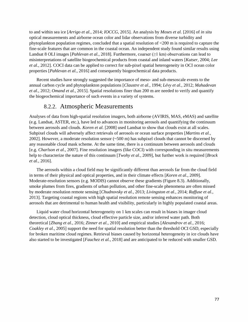
77

to and within sea ice [Arrigo et al., 2014; IOCCG, 2015]. An analysis by Moses et al. [2016] of in situ

optical measurements and airborne ocean color and lidar observations from diverse turbidity and

phytoplankton population regimes, concluded that a spatial resolution of <200 m is required to capture the

fine-scale features that are common in the coastal ocean. An independent study found similar results using

Landsat 8 OLI images [Pahlevan et al., 2018]. Furthermore, coarser (≥1 km) observations can lead to

misinterpretations of satellite biogeochemical products from coastal and inland waters [Kutser, 2004; Lee

et al., 2012]. COCI data can be applied to correct for sub-pixel spatial heterogeneity in OCI ocean color

properties [Pahlevan et al., 2016] and consequently biogeochemical data products.

Recent studies have strongly suggested the importance of meso- and sub-mesoscale events to the

annual carbon cycle and phytoplankton populations [Claustre et al., 1994; Lévy et al., 2012; Mahadevan

et al., 2012; Omand et al., 2015]. Spatial resolutions finer than 200 m are needed to verify and quantify

the biogeochemical importance of such events in a variety of systems.

8.2.2. Atmospheric Measurements

Analyses of data from high-spatial resolution imagers, both airborne (AVIRIS, MAS, eMAS) and satellite

(e.g. Landsat, ASTER, etc.), have led to advances in monitoring aerosols and quantifying the continuum

between aerosols and clouds. Koren et al. [2008] used Landsat to show that clouds exist at all scales.

Subpixel clouds will adversely affect retrievals of aerosols or ocean surface properties [Martins et al.,

2002]. However, a moderate resolution sensor (~500 m) has subpixel clouds that cannot be discerned by

any reasonable cloud mask scheme. At the same time, there is a continuum between aerosols and clouds

[e.g. Charlson et al., 2007]. Fine resolution imagers (like COCI) with corresponding in situ measurements

help to characterize the nature of this continuum [Twohy et al., 2009], but further work is required [Brock

et al., 2016].

The aerosols within a cloud field may be significantly different than aerosols far from the cloud field

in terms of their physical and optical properties, and in their climate effects [Koren et al., 2009].

Moderate-resolution sensors (e.g. MODIS) cannot observe these gradients (Figure 8.3). Additionally,

smoke plumes from fires, gradients of urban pollution, and other fine-scale phenomena are often missed

by moderate resolution remote sensing [Chudnovsky et al., 2013; Livingston et al., 2014; Raffuse et al.,

2013]. Targeting coastal regions with high spatial resolution remote sensing enhances monitoring of

aerosols that are detrimental to human health and visibility, particularly in highly populated coastal areas.

Liquid water cloud horizontal heterogeneity on 1 km scales can result in biases in imager cloud

detection, cloud optical thickness, cloud effective particle size, and/or inferred water path. Both

theoretical [Zhang et al., 2016; Zinner et al., 2010] and empirical studies [Alexandrov et al., 2016;

Coakley et al., 2005] support the need for spatial resolution better than the threshold OCI GSD, especially

for broken maritime cloud regimes. Retrieval biases caused by horizontal heterogeneity in ice clouds have

also started to be investigated [Fauchez et al., 2018] and are anticipated to be reduced with smaller GSD.

78

Science Questions Addressed by COCI

Top priority science questions that can be addressed with COCI data

• What are the spatial scales, composition, magnitudes and successional patterns of phytoplankton

populations, including blooms, in inland waters, estuaries, coastal ocean and open ocean, and how

are these phytoplankton populations driven by natural and human-induced change?

• How do the fine-scale (100-200 m) features of oceanic and coastal and inland water interfaces

(oceanic fronts, land-ocean, sea-ice margins, wetlands-estuary, river plumes, land-freshwater,)

contribute to regional and synoptic scale biogeochemical processes and associated distributions of

carbon, nutrients and sediments?

• How are water quality, water clarity, ecological integrity and trophic status being altered in

response to natural and human-induced change within inland waters, estuaries, nearshore and

coastal ocean waters both in managed and unmanaged systems?

• What are the spatial scales of variability of aerosols in the coastal zone and adjoining urban

centers and what are the implications for improving atmospheric correction in these zones and

understanding the impact on air quality and human health?

Other priority PACE-relevant science questions that can be addressed with COCI:

• How can data assimilation of high spatial resolution ocean color observations into models

improve model predictions of ocean physical and biogeochemical processes?

• Does the high productivity often observed in coastal, inland and estuarine waters alter aerosol

assemblages? If so, how significant are contributions from these waters to global inventories of

climate-relevant trace reactive gases and their radiative forcing?

• What are the characteristics of aerosols within a cloud field? Can we identify and then quantify

the radiative impacts of hydrated aerosols, cloud fragments versus adjacency effects? Can we

observe new particle generation in cloud fields? How do we quantify the continuum region, and

its associated effect on the radiative budget of Earth’s climate?

• How do fine-scale features of aerosol affect air quality in coastal urban environments, and how

does this play out in terms of public health and social justice?

• What fine-scale features of aerosol plumes can be linked to their sources, injection height and

transport predictability?

• What are the global areal extent, distribution, composition, status, and change in marshes,

mangrove forests, coral reefs and sea grass meadows? Climate change and intensifying pressures

of a growing human population are strongly impacting these ecosystems. Given large

uncertainties for the areal extent, distribution and loss rates of these vital habitats, it is critical and

urgent to establish an accurate baseline and to quantify change of coastal and inland aquatic

communities (emergent and benthic).

• What are the structural and biochemical characteristics of plant canopies? How are these

characteristics related to carbon, water, and energy fluxes? Can these characteristics describe plant

species and plant functional type diversity?

79

COCI Applied Science Objectives:

While the goal of COCI is to address these fundamental science questions the data will also be valuable

for NASA, NOAA, EPA, USGS, USFWS, BOEM, the U.S. Navy, numerous state and local agencies, as

well as Canadian and other international stakeholders to address key coastal and water resource

management objectives including:

• Identification of quantification of harmful algal blooms (HABs) and nuisance algal blooms

• Quantification and monitoring of water quality and clarity

• Enhanced precision/accuracy in water-quality products (e.g., phytoplankton abundance) in

lakes/reservoirs compared to that those from existing multispectral missions (e.g., Landsat)

• Determination of variability in phytoplankton biomass and community structure that are key to

developing improved ecosystem-based water quality and resource management strategies

• Understand spatio-temporal dynamics of lakes/reservoirs and plans for minimizing the

occurrences of major ecosystem disasters like fish-kill events

• Investigation of the link between terrestrial exports to eutrophication, HABs and hypoxia in

coastal zones

• Detection of changes in ice coverage, phytoplankton populations and associated biogeochemical

properties within coastal polynyas

• Detection and tracking of oil spills and seeps

• Development of indicators of water-borne pathogens

• Detection and quantification of event-scale features (responses to storms, upwelling, volcanic

eruptions, etc.) that impact annual primary productivity and biogeochemical cycles

• Mapping of marine protected areas and ecologically and biologically significant areas

• Mapping of preferred habitat for invasive species

• Characterization of fine-scale aerosol variability in urban and coastal zones that affect air quality

and impact human health

• Characterization of point source aerosol plumes (e.g., smoke)

• Characterization of terrestrial ecosystem diversity, biochemistry, and function

Summary

While PACE will continue our monitoring of the global ocean and atmosphere for the impacts of climate

change, COCI, with similar spectral capabilities and a spatial resolution that is 100 times finer (~0.01

km2) than OCI, takes us further into the near-shore ocean, estuaries, rivers and large lakes and reservoirs

where we are already seeing the impacts of human populations on a large scale on the water supply,

fisheries, air quality, recreational activities and human health for the majority of the world’s population

that lives near the coast.

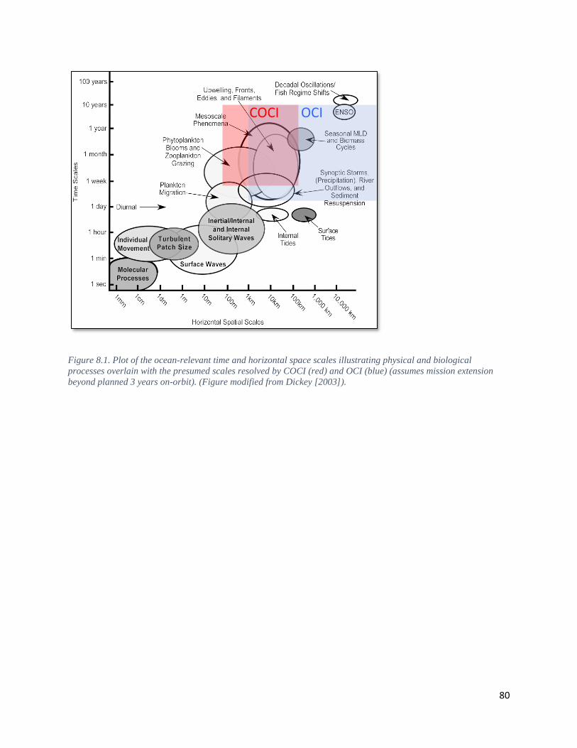
80

Figure 8.1. Plot of the ocean-relevant time and horizontal space scales illustrating physical and biological

processes overlain with the presumed scales resolved by COCI (red) and OCI (blue) (assumes mission extension

beyond planned 3 years on-orbit). (Figure modified from Dickey [2003]).

COCI OCI

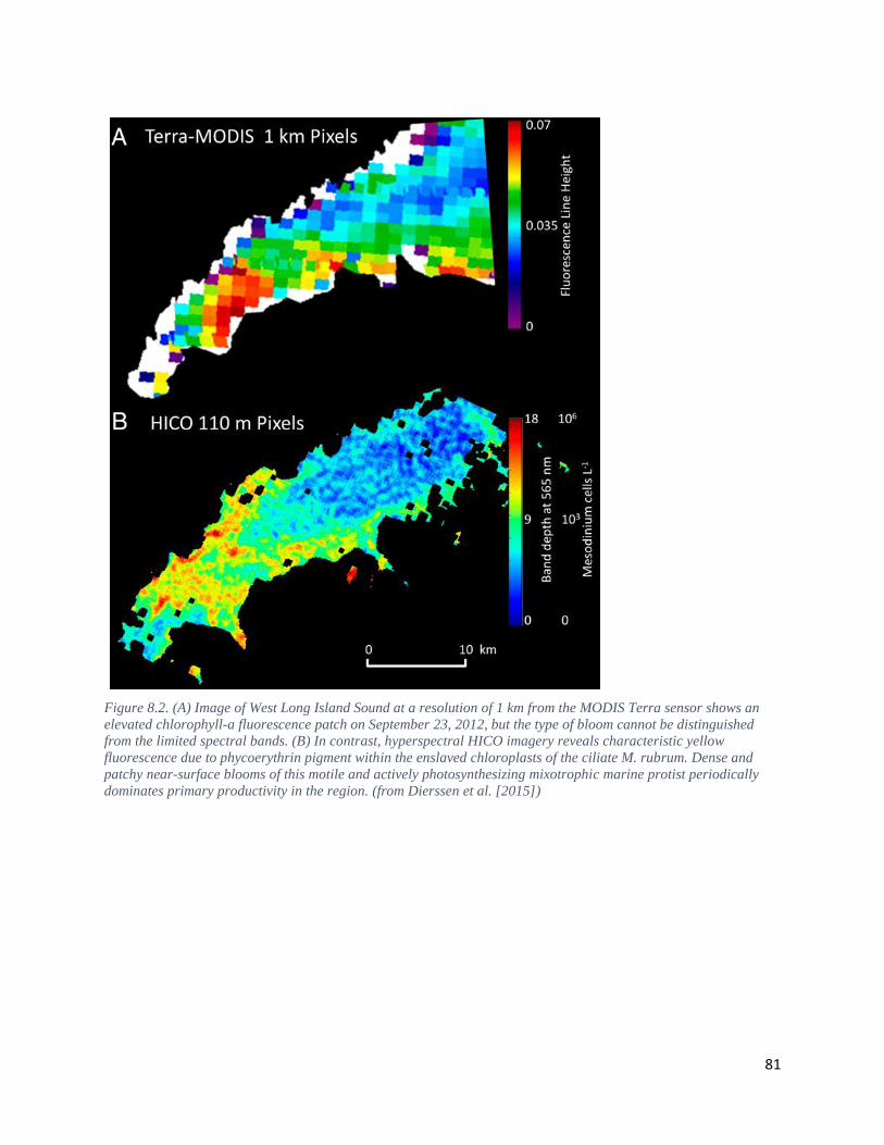
81

Figure 8.2. (A) Image of West Long Island Sound at a resolution of 1 km from the MODIS Terra sensor shows an

elevated chlorophyll-a fluorescence patch on September 23, 2012, but the type of bloom cannot be distinguished

from the limited spectral bands. (B) In contrast, hyperspectral HICO imagery reveals characteristic yellow

fluorescence due to phycoerythrin pigment within the enslaved chloroplasts of the ciliate M. rubrum. Dense and

patchy near-surface blooms of this motile and actively photosynthesizing mixotrophic marine protist periodically

dominates primary productivity in the region. (from Dierssen et al. [2015])

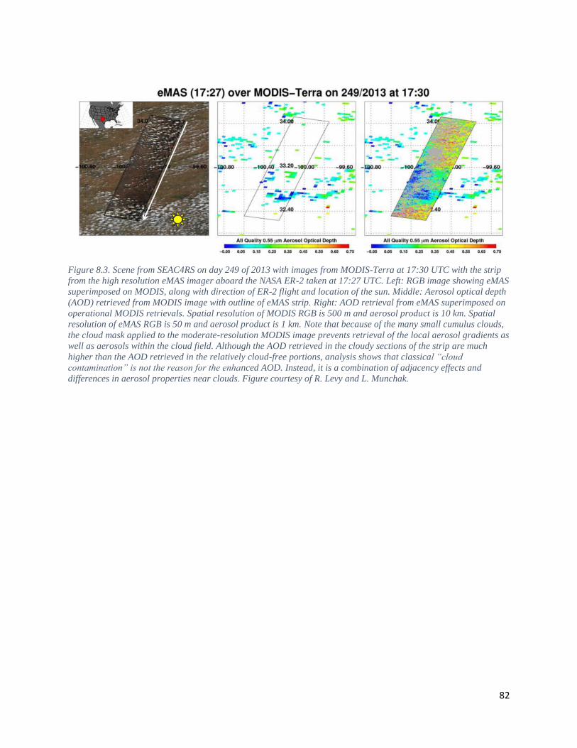
82

Figure 8.3. Scene from SEAC4RS on day 249 of 2013 with images from MODIS-Terra at 17:30 UTC with the strip

from the high resolution eMAS imager aboard the NASA ER-2 taken at 17:27 UTC. Left: RGB image showing eMAS

superimposed on MODIS, along with direction of ER-2 flight and location of the sun. Middle: Aerosol optical depth

(AOD) retrieved from MODIS image with outline of eMAS strip. Right: AOD retrieval from eMAS superimposed on

operational MODIS retrievals. Spatial resolution of MODIS RGB is 500 m and aerosol product is 10 km. Spatial

resolution of eMAS RGB is 50 m and aerosol product is 1 km. Note that because of the many small cumulus clouds,

the cloud mask applied to the moderate-resolution MODIS image prevents retrieval of the local aerosol gradients as

well as aerosols within the cloud field. Although the AOD retrieved in the cloudy sections of the strip are much

higher than the AOD retrieved in the relatively cloud-free portions, analysis shows that classical “cloud

contamination” is not the reason for the enhanced AOD. Instead, it is a combination of adjacency effects and

differences in aerosol properties near clouds. Figure courtesy of R. Levy and L. Munchak.

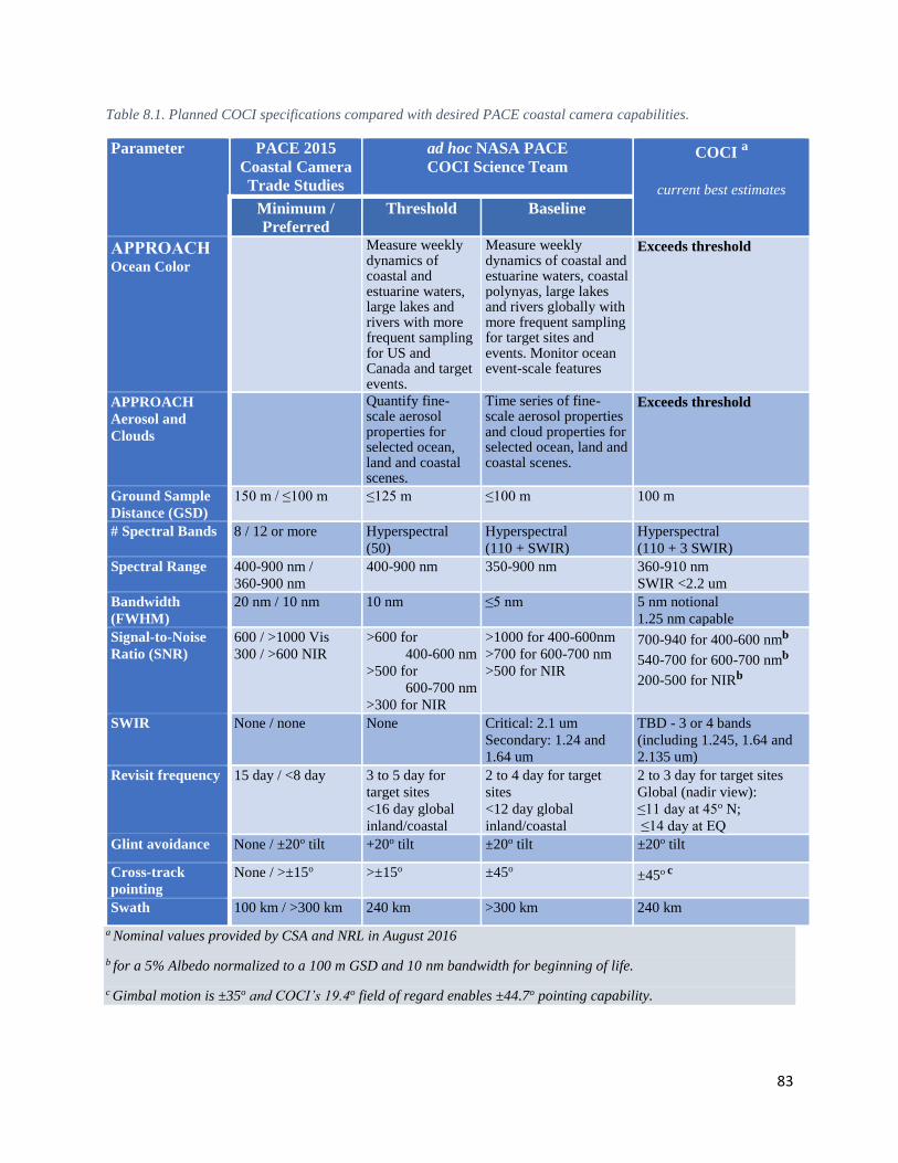
83

Table 8.1. Planned COCI specifications compared with desired PACE coastal camera capabilities.

Parameter PACE 2015

Coastal Camera

Trade Studies

ad hoc NASA PACE

COCI Science Team COCI

a

current best estimates

Minimum /

Preferred

Threshold Baseline

APPROACH Ocean Color

Measure weekly dynamics of coastal and estuarine waters, large lakes and rivers with more frequent sampling for US and Canada and target events.

Measure weekly dynamics of coastal and estuarine waters, coastal polynyas, large lakes and rivers globally with more frequent sampling for target sites and events. Monitor ocean event-scale features

Exceeds threshold

APPROACH

Aerosol and

Clouds

Quantify fine-scale aerosol properties for selected ocean, land and coastal scenes.

Time series of fine-scale aerosol properties and cloud properties for selected ocean, land and coastal scenes.

Exceeds threshold

Ground Sample

Distance (GSD)

150 m / ≤100 m ≤125 m ≤100 m 100 m

# Spectral Bands 8 / 12 or more Hyperspectral

(50)

Hyperspectral

(110 + SWIR)

Hyperspectral

(110 + 3 SWIR)

Spectral Range 400-900 nm /

360-900 nm

400-900 nm 350-900 nm 360-910 nm

SWIR <2.2 um

Bandwidth

(FWHM)

20 nm / 10 nm 10 nm ≤5 nm 5 nm notional

1.25 nm capable

Signal-to-Noise

Ratio (SNR)

600 / >1000 Vis

300 / >600 NIR

>600 for

400-600 nm

>500 for

600-700 nm

>300 for NIR

>1000 for 400-600nm

>700 for 600-700 nm

>500 for NIR

700-940 for 400-600 nmb

540-700 for 600-700 nmb

200-500 for NIRb

SWIR None / none None Critical: 2.1 um

Secondary: 1.24 and

1.64 um

TBD - 3 or 4 bands

(including 1.245, 1.64 and

2.135 um)

Revisit frequency 15 day / <8 day 3 to 5 day for

target sites

<16 day global

inland/coastal

2 to 4 day for target

sites

<12 day global

inland/coastal

2 to 3 day for target sites

Global (nadir view):

≤11 day at 45o N;

≤14 day at EQ

Glint avoidance None / ±20o tilt +20o tilt ±20o tilt ±20o tilt

Cross-track

pointing

None / >±15o >±15o ±45o ±45o c

Swath 100 km / >300 km 240 km >300 km 240 km

a Nominal values provided by CSA and NRL in August 2016

b for a 5% Albedo normalized to a 100 m GSD and 10 nm bandwidth for beginning of life.

c Gimbal motion is ±35o and COCI’s 19.4o field of regard enables ±44.7o pointing capability.

84

Appendix A

Table 8.2. Ad hoc NASA PACE COCI Science Team members.

NASA PACE COCI

Science Team Members

Affiliation Participated in 1st

COCI User and

Science Team

(June 1-2, 2016)

Brian Cairns NASA GSFC/GISS Yes

Curt Davis Oregon State University Yes (remotely)

Liane Guild NASA Ames No

Steven Lohrenz University of Massachusetts Dartmouth Yes

Antonio Mannino NASA GSFC Yes

Matthew Oliver University of Delaware Yes

Hans Paerl University of North Carolina Yes

Lorraine Remer University of Maryland Baltimore County Yes

Blake Schaeffer U.S. EPA Yes

Walker Smith Virginia Institute of Marine Science No

Rick Stumpf NOAA No

Maria Tzortziou City College of New York Yes

Jeremy Werdell NASA GSFC Yes

Richard Zimmerman Old Dominion University No

85

Table 8.3. Other contributors to science talking points white paper

Contributors Affiliation Member of PACE

Science Team

Steven Ackleson Narval Research Lab D.C. Yes

Martin Bergeron Canadian Space Agency No

Emmanuel Boss University of Maine Yes

Susanne Craig Dalhousie University Yes

Emmanuel Devred Fisheries and Oceans Canada No

Robert Frouin Scripps Institution of Oceanography Yes

Fred Huemmrich UMBC/NASA GSFC No

Zhongping Lee University of Massachusetts Yes

Rob Levy NASA GSFC Yes

Charles McClain Oregon State University No

Steve Platnick NASA GSFC Yes

Christopher Sioris Environment and Climate Change Canada No

Kevin Turpie UMBC/NASA GSFC No

Appendix B. PACE Mission Applications White Papers

pertaining to COCI

Harmful Algal Blooms (https://pace.oceansciences.org/docs/pace_oceans_white_paper_habs.pdf)

Air Quality (https://pace.oceansciences.org/docs/pace_atmos_white_paper_air_quality.pdf)

Marine ecosystem resources: Fisheries

(https://pace.oceansciences.org/docs/pace_oceans_white_paper_fisheries.pdf)

https://pace.oceansciences.org/docs/pace_oceans_white_paper_habs.pdf

https://pace.oceansciences.org/docs/pace_atmos_white_paper_air_quality.pdf

https://pace.oceansciences.org/docs/pace_oceans_white_paper_fisheries.pdf

86

Chapter 9

Analysis of a Pushbroom Ocean Color Instrument Lunar

Calibration

Frederick S. Patt, Science Applications International Corporation, Reston, Virginia8

9.

Executive Summary

During the PACE Pre-Phase A period, a study was performed of various instrument concepts for the

Ocean Color Instrument (OCI). One of the concepts studied was a pushbroom radiometer. PACE has a

Level 1 requirement to perform at least monthly lunar calibrations to track the temporal response of the

OCI. This paper presents an analysis of the requirements for performing a lunar calibration for the

pushbroom instrument concept for the OCI.

Introduction

The lunar calibration has been an integral element of the radiometric calibration methodology for every

NASA ocean color sensor since it was first used for the Sea-viewing Wide Field-of-view Sensor

(SeaWiFS) in 1997 [Eplee et al., 2012; Woodward et al., 1993]. Based on this highly successful track

record, PACE has a Level-1 requirement to perform OCI lunar calibrations. The threshold requirement is:

PACE shall provide:

g) Monthly characterizations of OCI instrument detector and optical component temporal stability. This

will include lunar observations through the earth viewing port that illuminate all detector elements

The baseline requirement is for two lunar calibrations per month, and is otherwise identical.

A pushbroom sensor has a linear array of detectors that view in the cross-track direction, imaging a

swath as the sensor (mounted on a spacecraft) moves in orbit. The OCI pushbroom concept instrument

had several thousand detectors in the array. This creates difficulties in performing a lunar calibration

operation to “illuminate all detector elements.”

The model of the lunar irradiance is provided by the Robotic Lunar Observatory (ROLO) model

developed by the U. S. Geological Survey [Kieffer and Stone, 2005]. The ROLO model provides the disk-

integrated irradiance (DII) to compare with the instrument observations of the Moon; this requires that the

instrument observations also be used to generate a DII. To satisfy the Level 1 requirement, a separate DII

would need to be generated for each detector in the pushbroom array, a very challenging requirement to

meet.

While pushbroom instruments have been used successfully for other disciplines (Land and

Atmosphere), they have not had the same calibration requirements as Ocean Color, and in general on-

8 Cite as: Patt, F. S. (2018), Analysis of a Pushbroom Ocean Color Instrument Lunar Calibration, in PACE Technical Report



87

orbit calibration approaches for existing pushbroom sensors do not address the requirements for Ocean

Color.

The following sections present the inputs that were used in this analysis; describe a maneuver

sequence that would meet the Level 1 requirement for all of the pushbroom detectors; discuss the analysis

that was performed to determine the requirements for the maneuvers; present the impacts to the mission;

and summarize the key requirements.

9.1.1. Inputs

The objective of the maneuver sequence is to collect a full-disk lunar image for every cross-track IFOV

(i.e., detector) of the instrument, with an accuracy and consistency that meets the overall requirements for

temporal calibration response (0.1%).

The diameter of the Moon is 3475 km, and the Earth-Moon distance ranges from about 356,000 to

414,000 km. Since the lunar measurements will be performed during the orbit nighttime, the spacecraft-

Moon distance will be less than this by up to the orbit radius, 7193 km.

The total cross-track FOV of the instrument is 104 degrees.

The IFOV is 297.48 μradian (0.017044 degree, about 1 arcminute). The sample interval is 0.039

seconds. The same sampling will be used for the lunar measurements as for the Earth data collection.

The orbit altitude is 815 km, corresponding to an orbit period of 6072 seconds.

The Earth data collection will be performed to cover the solar zenith angle range to 75 degrees,

corresponding to 2530 seconds of the orbit. This leaves 3542 seconds, or about 59 minutes, for the lunar

calibration operations during each orbit. If the maneuvers are timed to the terminator crossings, then 50.5

minutes is available.

The spacecraft is capable of inertial slew rates of up to 2 degree/sec. It takes 180 seconds to achieve

that rate starting from 0, corresponding to an angular acceleration of 2/180 (~0.01111111) degree/sec2.

The acceleration is assumed to be linear. Note that while accelerating from 0 to 2 degree/sec, the

spacecraft would rotate by 180 degrees, so for smaller maneuvers the maximum rate would not be

achieved; the ADCS would accelerate at the maximum rate up to the midpoint of the maneuver and

decelerate to the end.

The estimated control accuracy is about 1.2 arcminutes (1 sigma), approximately equivalent to 1

IFOV.

9.1.2. Maneuver Sequence

The proposed maneuver sequence is as follows:

1. After the end of Earth data collection, the spacecraft is pitched to position the pushbroom FOV just

above the Moon, and rolled to position it to one side of the Moon.

2. The spacecraft begins a roll/pitch raster maneuver sequence, to cause the entire pushbroom array to

view successive "slices" of the Moon. For each slice, the spacecraft is held at a constant inertial pitch and

maneuvered in roll to cause the entire array to view the Moon. The roll maneuver is then stopped, the

pitch is incremented by one IFOV, and the roll maneuver is repeated in the opposite direction. This

sequence is illustrated in Figure 9.1.

88

3. As the spacecraft approaches the start of Earth data collection, it is pitched to nadir, with time for

settling before the start of collection.

4. This sequence is repeated for successive orbits to view the entire Moon. At the start of each orbit's

raster sequence, the pushbroom FOV is positioned to perform the raster for the next slice after the last one

from the previous orbit.

Figure 9.1. Sequence of Raster Maneuvers

Analysis

The key elements of the proposed lunar calibration maneuver sequence are: the time required; the

maneuver accuracy and stability; geometry and viewing conditions that can affect the observations; and

the non-uniformity of the lunar disk. Each of these is discussed below.

9.2.1. Timing

If the pitch maneuver is started immediately after the end of Earth data collection (15 degrees before the

terminator crossing), the average pitch maneuver will be 75 degrees. Based on the angular acceleration

rate, this would take 165 seconds. This maneuver would also be performed before the start of the next

Earth data collection, for a total of 330 seconds. This allows 53.5 minutes between the maneuvers.

If the maneuver is delayed to the terminator crossing, the average pitch would be 90 degrees, which

would take 180 seconds. This allows 47.5 minutes between pitch maneuvers.

The required roll rate during the raster maneuver is one IFOV per sample period, which corresponds

to 0.437 degree/sec. To view the lunar disk using the 104-deg FOV at that rate will require 4 minutes. The

time required to reverse the roll rate will be 79 seconds, so the total time for each raster is about 5 minutes

20 seconds.

Moon

89

The time available to perform the rasters depends on the timing of the pitch maneuvers, and also

whether there is a requirement to perform the lunar observations in eclipse. The eclipse period is 35

minutes per orbit. The number of rasters per orbit for each case is as follows:

53.5 minutes 10 rasters

47.5 minutes 9 rasters

35 minutes 6 rasters

The maximum size of the lunar disk is 0.00993 radian (0.569 degree). This means that it will require

up to 34 rasters to view the entire disk. At 9 rasters/orbit, four orbits will be required; this will also allow

one raster above and below the disk to ensure that a full-disk image is collected. At 6 rasters per orbit, six

orbits will be required.

9.2.2. Maneuver Accuracy and Stability

The requirement is to collect full-disk images for every detector with high consistency places stringent

requirements on the raster maneuver accuracy and stability. The Moon is a significantly non-uniform

source, which is why the approach using full-disk images has been used for heritage missions.

Given the duration of each raster, the roll rate will need to be either maintained or measured to the

required consistency (0.1%). At the roll rate of 0.437 degree/sec, or 1573 arcsecond/sec, the required

stability or knowledge is 1.6 arcsecond/sec. While it is probably difficult to maintain the roll rate at that

accuracy, it should be possible to measure it using gyro data, and correct the lunar disk images for each

detector using the gyro data.

Pointing control during the maneuvers is more problematic. The lunar disk is not a uniform source,

and therefore variations in the pointing control during the maneuvers will cause variations in the

radiometric measurements among the detectors. Potential error sources are:

1. Pitch and yaw deviations. To collect uniform slices of the Moon, the pitch angle increments between

rasters need to be equally uniform, and the yaw angle needs to be controlled as well. Deviations in the

pitch angle increments will cause nonuniform sampling of the disk across all of the rasters, and deviations

in yaw will cause variations among detectors during a raster. The specific control requirements will more

stringent than the requirements for Earth data collection, which allow control errors of about 2 IFOV. The

effects of these deviations on lunar disk sampling are illustrated in Figure 9.2.

2. Pitch and yaw stability. Variations in the pitch or yaw angles during a raster would also result in

nonuniform sampling of the disk among the detectors.

3. Maneuver axis variations. Deviations of the raster maneuver axis from the spacecraft roll axis would

cause variations in the effective pitch and/or yaw angles during the raster.

Note that for any of these, pointing knowledge cannot be used to rectify the lunar disk images to

account for pointing control errors.

9.2.3. Geometry and Viewing

There are three issues that arise in the geometry of the lunar view during the maneuvers, due to the time

required.

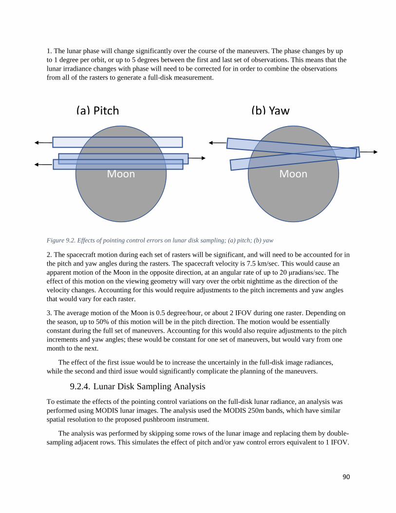
90

1. The lunar phase will change significantly over the course of the maneuvers. The phase changes by up

to 1 degree per orbit, or up to 5 degrees between the first and last set of observations. This means that the

lunar irradiance changes with phase will need to be corrected for in order to combine the observations

from all of the rasters to generate a full-disk measurement.

Figure 9.2. Effects of pointing control errors on lunar disk sampling; (a) pitch; (b) yaw

2. The spacecraft motion during each set of rasters will be significant, and will need to be accounted for in

the pitch and yaw angles during the rasters. The spacecraft velocity is 7.5 km/sec. This would cause an

apparent motion of the Moon in the opposite direction, at an angular rate of up to 20 μradians/sec. The

effect of this motion on the viewing geometry will vary over the orbit nighttime as the direction of the

velocity changes. Accounting for this would require adjustments to the pitch increments and yaw angles

that would vary for each raster.

3. The average motion of the Moon is 0.5 degree/hour, or about 2 IFOV during one raster. Depending on

the season, up to 50% of this motion will be in the pitch direction. The motion would be essentially

constant during the full set of maneuvers. Accounting for this would also require adjustments to the pitch

increments and yaw angles; these would be constant for one set of maneuvers, but would vary from one

month to the next.

The effect of the first issue would be to increase the uncertainly in the full-disk image radiances,

while the second and third issue would significantly complicate the planning of the maneuvers.

9.2.4. Lunar Disk Sampling Analysis

To estimate the effects of the pointing control variations on the full-disk lunar radiance, an analysis was

performed using MODIS lunar images. The analysis used the MODIS 250m bands, which have similar

spatial resolution to the proposed pushbroom instrument.

The analysis was performed by skipping some rows of the lunar image and replacing them by double-

sampling adjacent rows. This simulates the effect of pitch and/or yaw control errors equivalent to 1 IFOV.

Moon Moon

(a) Pitch (b) Yaw

91

The results of the analysis showed variations in the disk-integrated radiances of up to 1%. If the

average value was about 0.5%, this analysis indicates that in order to reduce the variations to 0.1%, the

control accuracy would need to be equivalent to 0.2 IFOV, or about 0.2 arcminute (12 arcseconds).

Mission Impacts

The performance of the pushbroom lunar calibration would result in both technical and cost impacts to the

mission.

There were two proposals for performing the raster maneuvers:

• The spacecraft ADCS performs all pitch and roll maneuvers required. This would require

significant augmentation of the ADCS to achieve the required accuracy.

• The instrument could be mounted on a two-axis gimbal, which would perform the pitch and roll

rasters. The spacecraft would perform pitch maneuver to point nadir axis at Moon. This would

require real-time feedback of pointing errors to gimbal controls to maintain pointing accuracy,

and might also require a dedicated star tracker to maintain pointing knowledge during rasters.

Both of these would have cost impacts, which were not estimated as part of this study.

The maneuvers would also require significant operational efforts, resulting in further cost impact.

Each calibration requires a complicated sequence of pitch and raster maneuvers and up to six orbits per

monthly calibration event. This would require a significant planning and operations effort each month to

carry out the required set of maneuvers. It was estimated that at least one additional FTE per year would

be required to plan and execute the monthly calibration maneuvers, compared to the effort required for a

scanning instrument. In addition, at least two additional FTEs per year would be required to perform

additional data analyses (~6000 detectors).

Summary of Key Requirements

The proposed lunar calibration activity for the ocean color pushbroom instrument is designed to obtain

full-disk images for every detector in the pushbroom array. The combination of pitch and raster

maneuvers that are required to accomplish this are complicated, and would take four to six orbits per

monthly calibration event.

The requirement for 0.1% consistency across all of the detectors places very stringent requirements

on the pointing control accuracy during the raster maneuvers. An analysis based on MODIS lunar

calibration images indicates that control accuracy of 0.2 arcminute would be required to meet the

radiometric requirement.

In addition, the geometric viewing conditions will change significantly during each orbit (due to the

spacecraft velocity) and for each calibration event (due to the Moon's motion). This will require extensive

planning of the raster maneuvers for each calibration event in order to achieve the required consistency of

the lunar images.

92

References

Alexandrov, M. D., B. Cairns, B. van Diedenhoven, A. S. Ackerman, A. P. Wasilewski, M. J. McGill, J.

E. Yorks, D. L. Hlavka, S. E. Platnick, and G. T. Arnold (2016), Polarized view of supercooled liquid

water clouds, Remote Sens. Environ., 181, 96-110, doi:https://doi.org/10.1016/j.rse.2016.04.002.

Archer, C. L., and M. Z. Jacobson (2005), Evaluation of global wind power, Journal of Geophysical

Research: Atmospheres, 110(D12), doi:doi:10.1029/2004JD005462.

Arrigo, K. R., et al. (2014), Phytoplankton blooms beneath the sea ice in the Chukchi Sea, Deep Sea

Research Part II: Topical Studies in Oceanography, 105(0), 1-16,

doi:http://dx.doi.org/10.1016/j.dsr2.2014.03.018.

Behrenfeld, M. J., Y. Hu, C. A. Hostetler, G. Dall'Olmo, S. D. Rodier, J. W. Hair, and C. R. Trepte

(2013), Space‐based lidar measurements of global ocean carbon stocks, Geophys. Res. Lett., 40(16),

4355-4360.

Behrenfeld, M. J., et al. (2016), Annual boom–bust cycles of polar phytoplankton biomass revealed by

space-based lidar, Nature Geoscience, 10, 118, doi:10.1038/ngeo2861.

Bélanger, S., J. K. Ehn, and M. Babin (2007), Impact of sea ice on the retrieval of water-leaving

reflectance, chlorophyll a concentration and inherent optical properties from satellite ocean color data,

Remote Sensing of Environment, 111(1), 51-68, doi:http://dx.doi.org/10.1016/j.rse.2007.03.013.

Bézy, J.-L., S. Delwart, and M. Rast (2000), MERIS – A New Generation of Ocean Colour Sensor

onboard Envisat, ESA Bulletin(103), 48-56.

Bouvet, M., and F. Ramino (2009), Equalization of MERIS L1b products from the 2nd reprocessingRep.,

ESA.

Brekke, C., and A. H. S. Solberg (2005), Oil spill detection by satellite remote sensing, Remote Sens.

Environ., 95(1), 1-13, doi:https://doi.org/10.1016/j.rse.2004.11.015.

Bricaud, A., A. Morel, M. Babin, K. Allali, and H. Claustre (1998), Variations of light absorption by

suspended particles with the chlorophyll a concentration in oceanic (Case 1) waters : analysis and

implications for bio-optical models, J. Geophys. Res. Oceans, 103, 31033-31044.

Brock, C. A., N. L. Wagner, B. E. Anderson, A. R. Attwood, A. Beyersdorf, P. Campuzano-Jost, A. G.

Carlton, D. A. Day, G. S. Diskin, and T. D. Gordon (2016), Aerosol optical properties in the southeastern

United States in summer–Part 1: Hygroscopic growth, Atmospheric Chemistry and Physics, 16(8), 4987-

5007.

Bulgarelli, B., V. Kiselev, and G. Zibordi (2014), Simulation and analysis of adjacency effects in coastal

waters: a case study, Appl. Optics, 53(8), 1523-1545.

Charlson, R. J., A. S. Ackerman, F. A.-M. Bender, T. L. Anderson, and Z. Liu (2007), On the climate

forcing consequences of the albedo continuum between cloudy and clear air, Tellus B: Chemical and

Physical Meteorology, 59(4), 715-727.

Chudnovsky, A. A., A. Kostinski, A. Lyapustin, and P. Koutrakis (2013), Spatial scales of pollution from

variable resolution satellite imaging, Environ Pollut, 172, 131-138, doi:10.1016/j.envpol.2012.08.016.

Claustre, H., P. Kerherve, J. C. Marty, and L.Prieur (1994), Phytoplankton adaptation related to some

frontal physical processes, J. Mar. Syst., 5, 251-265.

93

Coakley, J. A., M. A. Friedman, and W. R. Tahnk (2005), Retrieval of Cloud Properties for Partly Cloudy

Imager Pixels, Journal of Atmospheric and Oceanic Technology, 22(1), 3-17, doi:10.1175/jtech-1681.1.

Corsini, G., M. Diani, and T. Walzel (2000), Striping removal in MOS-B data, IEEE Transactions on

Geoscience and Remote Sensing, 38(3), 1439-1446, doi:10.1109/36.843038.

Cox, C., and W. Munk (1954), Measurement of the Roughness of the Sea Surface from Photographs of

the Sun’s Glitter, J. Opt. Soc. Am., 44(11), 838-850, doi:10.1364/JOSA.44.000838.

Craig, S. E., S. E. Lohrenz, Z. Lee, K. L. Mahoney, G. J. Kirkpatrick, O. M. Schofield, and R. G. Steward

(2006), Use of hyperspectral remote sensing reflectance for detection and assessment of the harmful alga,

Karenia brevis, Appl. Opt., 45(21), 5414-5425, doi:10.1364/AO.45.005414.

Dickey, T. D. (2003), Emerging ocean observations for interdisciplinary data assimilation systems, J.

Mar. Syst., 40, 5-48.

Dierssen, H., G. B. McManus, A. Chlus, D. Qiu, B.-C. Gao, and S. Lin (2015), Space station image

captures a red tide ciliate bloom at high spectral and spatial resolution, Proceedings of the National

Academy of Sciences, 112(48), 14783-14787, doi:10.1073/pnas.1512538112.

Eplee, R. E., G. Meister, F. S. Patt, R. A. Barnes, S. W. Bailey, B. A. Franz, and C. R. McClain (2012),

On-orbit calibration of SeaWiFS, Appl. Opt., 51(36), 8702-8730, doi:10.1364/AO.51.008702.

Fauchez, T., S. Platnick, O. Sourdeval, C. Wang, K. Meyer, C. Cornet, and F. Szczap (2018), Cirrus

Horizontal Heterogeneity and 3-D Radiative Effects on Cloud Optical Property Retrievals From MODIS

Near to Thermal Infrared Channels as a Function of Spatial Resolution, Journal of Geophysical Research:

Atmospheres, 123(19), 11,141-111,153, doi:doi:10.1029/2018JD028726.

Franz, B. A. (1998), A Simple Destriping Algorithm for MOS ImagesRep., NASA/SIMBIOS Project

https://oceancolor.gsfc.nasa.gov/staff/franz/papers/franz_1998_mosberlin.pdf.

Franz, B. A., S. W. Bailey, N. Kuring, and P. J. Werdell (2015), Ocean color measurements with the

Operational Land Imager on Landsat-8: implementation and evaluation in SeaDAS, Journal of Applied

Remote Sensing, 9(1), 096070-096070.

Gordon, H. R., O. B. Brown, R. H. Evans, J. W. Brown, R. C. Smith, K. S. Baker, and D. K. Clark

(1988), A Semianalytic Radiance Model of Ocean Color, Journal of Geophysical Research, 93(D9),

10909-10924.

Gregg, W. W., and F. S. Patt (1994), Assessment of tilt capability for spaceborne global ocean color

sensors, IEEE Transactions on Geoscience and Remote Sensing, 32(4), 866-877, doi:10.1109/36.298014.

Group, A. O. W. (2018), ACE Ocean Working Group recommendations and instrument requirements for

an advanced ocean ecology missionRep., NASA Goddard Space Flight Center, Greenbelt, MD.

Hestir, E. L., V. E. Brando, M. Bresciani, C. Giardino, E. Matta, P. Villa, and A. G. Dekker (2015),

Measuring freshwater aquatic ecosystems: The need for a hyperspectral global mapping satellite mission,

Remote Sens. Environ., 167, 181-195, doi:http://dx.doi.org/10.1016/j.rse.2015.05.023.

Hu, C., L. Feng, Z. Lee, C. O. Davis, A. Mannino, C. R. McClain, and B. A. Franz (2012), Dynamic

range and sensitivity requirements of satellite ocean color sensors: learning from the past, Appl. Opt.,

51(25), 6045-6062, doi:10.1364/AO.51.006045.

IOCCG (1999), Status and Plans for Satellite Ocean-Colour Missions: Considerations for

Complementary Missions, IOCCG Dartmouth,, Canada.

94

IOCCG (2006), Remote Sensing of Inherent Optical Properties: Fundamentals, Tests of Algorithms, and

Applications, IOCCG, Dartmouth, Canada.

IOCCG (2015), Ocean Colour Remote Sensing in Polar Seas, IOCCG Dartmouth,, Canada.

Kieffer, H. H., and T. C. Stone (2005), The Spectral Irradiance of the Moon, The Astronomical Journal,

129(6), 2887.

Koren, I., G. Feingold, H. Jiang, and O. Altaratz (2009), Aerosol effects on the inter‐cloud region of a

small cumulus cloud field, Geophys. Res. Lett., 36(14).

Koren, I., L. Oreopoulos, G. Feingold, L. Remer, and O. Altaratz (2008), How small is a small cloud?,

Atmospheric Chemistry and Physics, 8(14), 3855-3864.

Kutser, T. (2004), Quantitative detection of chlorophyll in cyanobacterial blooms by satellite remote

sensing, Limnol. Oceanogr., 49(6), 2179-2189.

Lee, Z., C. Hu, R. Arnone, and Z. Liu (2012), Impact of sub-pixel variations on ocean color remote

sensing products, Opt. Express, 20(19), 20844-20854, doi:10.1364/OE.20.020844.

Lee, Z., C. Hu, B. Casey, S. Shang, H. Dierssen, and R. Arnone (2010), Global Shallow—Water

Bathymetry From Satellite Ocean Color Data, Eos, Transactions American Geophysical Union, 91(46),

429-430.

Lee, Z. P., K. L. Carder, and R. A. Arnone (2002), Deriving inherent optical properties from water color:

a multiband quasi-analytical algorithm for optically deep waters, Appl. Opt., 41, 5755-5772.

Lévy, M., R. Ferrari, P. J. S. Franks, A. P. Martin, and P. Rivière (2012), Bringing physics to life at the

submesoscale, Geophys. Res. Lett., 39(14), L14602, doi:10.1029/2012GL052756.

Livingston, J., J. Redemann, Y. Shinozuka, R. Johnson, P. Russell, Q. Zhang, S. Mattoo, L. Remer, R.

Levy, and L. Munchak (2014), Comparison of MODIS 3 km and 10 km resolution aerosol optical depth

retrievals over land with airborne sunphotometer measurements during ARCTAS summer 2008,

Atmospheric Chemistry and Physics, 14(4), 2015-2038.

Lubac, B., H. Loisel, N. Guiselin, R. Astoreca, L. Felipe Artigas, and X. Mériaux (2008), Hyperspectral

and multispectral ocean color inversions to detect Phaeocystis globosa blooms in coastal waters, Journal

of Geophysical Research: Oceans, 113(C6), doi:10.1029/2007JC004451.

Lyon, P. E. (2009), An automated de‐striping algorithm for Ocean Colour Monitor imagery, International

Journal of Remote Sensing, 30(6), 1493-1502, doi:10.1080/01431160802468263.

Mahadevan, A., E. D’Asaro, C. Lee, and M. J. Perry (2012), Eddy-Driven Stratification Initiates North

Atlantic Spring Phytoplankton Blooms, Science, 337(6090), 54-58, doi:10.1126/science.1218740.

Martins, J. V., D. Tanré, L. Remer, Y. Kaufman, S. Mattoo, and R. Levy (2002), MODIS cloud screening

for remote sensing of aerosols over oceans using spatial variability, Geophysical Research Letters,

29(12), MOD4-1-MOD4-4.

McClain, C., et al. (2012), The Ocean Radiometer for Carbon Assessment (ORCA): Development History

within and Advanced Ocean Mission Concept, Science Objectives, Design Rationale, and Sensort

Prototype Description, NASA/TM-2012-215894Rep., NASA Goddard Space Flight Center, Greenbelt,

MD.

McClain, C. R., G. Meister, and B. Monosmith (2014), Chapter 2.1 - Satellite Ocean Color Sensor Design

Concepts and Performance Requirements, in Experimental Methods in the Physical Sciences, edited by G.

95

Zibordi, C. J. Donlon and A. C. Parr, pp. 73-119, Academic Press, doi:https://doi.org/10.1016/B978-0-12-

417011-7.00005-2.

McKinna, L. I. W., R. Lossing, and J. Werdell (2018), Assessment of hyperspectral pushbroom image

striping artifacts in ocean color products, in PACE Technical Report Series, Volume 5: Mission

Formulation Studies (NASA/TM-2018 – 2018-219027/ Vol. 5), edited by I. Cetinić, C. R. McClain and P.

J. Werdell, NASA Goddard Space Flight Space Center Greenbelt, MD.

Moses, W. J., S. G. Ackleson, J. W. Hair, C. A. Hostetler, and W. D. Miller (2016), Spatial scales of

optical variability in the coastal ocean: Implications for remote sensing and in situ sampling, Journal of

Geophysical Research: Oceans, n/a-n/a, doi:10.1002/2016JC011767.

Mouw, C. B., et al. (2015), Aquatic color radiometry remote sensing of coastal and inland waters:

Challenges and recommendations for future satellite missions, Remote Sens. Environ., 160(0), 15-30,

doi:10.1016/j.rse.2015.02.001.

NASA (2010), Responding to the Challenge of Climate and Environmental Change: NASA’s Plan for a

Climate-Centric Architecture for Earth Observations and Applications from Space, edited, p. 48.

O'Reilly, J., E., S. Maritorena, B. G. Mitchell, D. Siegel, A., K. Carder, L., S. Garver, A., M. Kahru, and

C. McClain (1998), Ocean color chlorophyll algorithms for SeaWiFS, Journal of Geophysical Research:

Oceans, 103(C11), 24937-24953, doi:10.1029/98JC02160.

Omand, M. M., E. A. D’Asaro, C. M. Lee, M. J. Perry, N. Briggs, I. Cetinić, and A. Mahadevan (2015),

Eddy-driven subduction exports particulate organic carbon from the spring bloom, Science, 348(6231),

222-225, doi:10.1126/science.1260062.

Pahlevan, N., S. Sarkar, and B. A. Franz (2016), Uncertainties in coastal ocean color products: Impacts of

spatial sampling, Remote Sens. Environ., 181, 14-26.

Pahlevan, N., S. R. Signorini, and I. Cetinić (2018), Estimating coastal ocean feature sizes for optimal

remote sensing of coastal waters, in PACE Technical Report Series, Volume 7: Ocean Color Instrument

(OCI) Concept Design Studies (NASA/TM-2018 – 2018-219027/ Vol. 7), edited by I. Cetinić, C. R.

McClain and P. J. Werdell, NASA Goddard Space Flight Space Center Greenbelt, MD.

Pande-Chhetri, R., and A. Abd-Elrahman (2011), De-striping hyperspectral imagery using wavelet

transform and adaptive frequency domain filtering, ISPRS Journal of Photogrammetry and Remote

Sensing, 66(5), 620-636, doi:https://doi.org/10.1016/j.isprsjprs.2011.04.003.

Pande-Chhetri, R., and A. Abd-Elrahman (2013), Filtering high-resolution hyperspectral imagery in a

maximum noise fraction transform domain using wavelet-based de-striping, International Journal of

Remote Sensing, 34(6), 2216-2235, doi:10.1080/01431161.2012.742592.

Patt, F. (2002), Navigation algorithms for the SeaWiFS missionRep., NASA GSFC, Greenbelt, USA.

Patt, F. S. (2018), Analysis of a Pushbroom Ocean Color Instrument Lunar Calibration, in PACE

Technical Report Series, Volume 5: Mission Formulation Studies (NASA/TM-2018 – 2018-219027/ Vol.

5), edited by I. Cetinić, C. R. McClain and P. J. Werdell, NASA Goddard Space Flight Space Center

Greenbelt, MD.

Patt, F. S., and W. W. Gregg (1994), Exact closed-form geolocation algorithm for Earth survey sensors,

Int. J. Remote Sens., 15(18), 3719-3734, doi:10.1080/01431169408954354.

96

Raffuse, S. M., M. C. McCarthy, K. J. Craig, J. L. DeWinter, L. K. Jumbam, S. Fruin, W. James

Gauderman, and F. W. Lurmann (2013), High‐resolution MODIS aerosol retrieval during wildfire events

in California for use in exposure assessment, Journal of Geophysical Research: Atmospheres, 118(19),

11,242-211,255.

PACE Science Definition Team (2018), Pre-Aerosol, Clouds, and ocean Ecosystem (PACE) Mission

Science Definition Team ReportRep., NASA Goddard Space Flight Center, Greenbelt, MD.

Twohy, C. H., J. A. Coakley Jr, and W. R. Tahnk (2009), Effect of changes in relative humidity on

aerosol scattering near clouds, Journal of Geophysical Research: Atmospheres, 114(D5).

Tzortziou, M., P. J. Neale, J. P. Megonigal, C. L. Pow, and M. Butterworth (2011), Spatial gradients in

dissolved carbon due to tidal marsh outwelling into a Chesapeake Bay estuary, Mar. Ecol. Prog. Ser.,

426, 41-56.

Vane, G., R. O. Green, T. G. Chrien, H. T. Enmark, E. G. Hansen, and W. M. Porter (1993), The airborne

visible/infrared imaging spectrometer (AVIRIS), Remote Sens. Environ., 44(2-3), 127-143.

Verpoorter, C., T. Kutser, D. A. Seekell, and L. J. Tranvik (2014), A global inventory of lakes based on

high‐resolution satellite imagery, Geophys. Res. Lett., 41(18), 6396-6402.

Wang, M., and S. W. Bailey (2001), Correction of sun glint contamination on the SeaWiFS ocean and

atmosphere products, Appl. Opt., 40(27), 4790-4798, doi:10.1364/AO.40.004790.

Werdell, P. J. (2018), PACE Ocean Color Science Data Product Requirements, in PACE Technical

Report Series, Volume 6: Data Product Requirements and Error Budgets (NASA/TM-2018 – 2018-

219027/ Vol. 6), edited by I. Cetinić, C. R. McClain and P. J. Werdell, NASA Goddard Space Flight

Space Center Greenbelt, MD.

Werdell, P. J., et al. (2013), Generalized ocean color inversion model for retrieving marine inherent

optical properties, Appl. Opt., 52(10), 2019-2037, doi:10.1364/AO.52.002019.

Woodward, R. H., R. A. Barnes, C. R. McClain, W. E. Esaias, W. L. Barnes, and A. Mecherikunnel

(1993), SeaWiFS Technical Report Series: Modeling of the SeaWiFS Solar and Lunar ObservationsRep.,

26 pp, NASA Goddard Space Flight Center, Greenbelt, Maryland.

Xi, H., M. Hieronymi, R. Röttgers, H. Krasemann, and Z. Qiu (2015), Hyperspectral Differentiation of

Phytoplankton Taxonomic Groups: A Comparison between Using Remote Sensing Reflectance and

Absorption Spectra, Remote Sensing, 7(11), doi:10.3390/rs71114781.

Zhang, Z., F. Werner, H.-M. Cho, G. Wind, S. Platnick, A. S. Ackerman, L. Di Girolamo, A. Marshak,

and K. Meyer (2016), A framework based on 2-D Taylor expansion for quantifying the impacts of

subpixel reflectance variance and covariance on cloud optical thickness and effective radius retrievals

based on the bispectral method, Journal of Geophysical Research: Atmospheres, 121(12), 7007-7025,

doi:doi:10.1002/2016JD024837.

Zinner, T., G. Wind, S. Platnick, and A. Ackerman (2010), Testing remote sensing on artificial

observations: impact of drizzle and 3-D cloud structure on effective radius retrievals, Atmospheric

Chemistry and Physics, 10(19), 9535-9549.

Previous Volumes in This Series

Volume 1

April 2018

ACE Ocean Working Group recommendations and instrument

requirements for an advanced ocean ecology mission

Volume 2

May 2018

Pre-Aerosol, Clouds, and ocean Ecosystem (PACE) Mission

Science Definition Team Report

Volume 3

October 2018

Polarimetry in the PACE mission: Science Team consensus document

Volume 4

October 2018

Cloud retrievals in the PACE mission: Science Team consensus document

Documents

Ivona Cetinić, Charles R. McClain, and P. Jeremy Werdell