John Riley minor corrections 25 July 2016

Concave functions in economics

1. Preliminaries 1

2. Concave function of one variable 4

3. Concave function of more than one variable 7

4. Necessary and sufficient conditions for a maximum 10

5. When is a function concave 11

6. The gains to diversifying 15

7. Production plans and supporting prices 17

8. Constrained maximization 22

25 pages

John Riley

1

Maximization with concave functions

Elsewhere module we have discussed necessary conditions for a maximum for the

following problem:

{ ( ) | }n

xMax f x x

As long as the set of vectors satisfying the necessary conditions is small, it is in principle

possible to solve by computing the value of f for each such vector and hence solve for the one

that is the global maximizer.

With concave functions, solving maximization problems is so much easier. If you can find

a vector satisfying the first order conditions for a maximum, then you have found the solution.

It is therefore very important to have a strong understanding of concave functions.

1. Preliminaries

Line through a in the direction of b

Consider the vector x a b . This is depicted below for three values of . As is clear from

the figure, the graph of ( )x is a line in 2 through the vector a in the direction of b .

Similarly, if a and 3b , then ( )x a b is a line in 3 . For higher dimensions we keep

this same terminology.

Fig.1-1: Line through in the direction of

John Riley

2

Line through 0a and 1a

As argued above, 0 1 0( ) ( )x a a a is a line through 0a in the direction of 1 0a a . Since

1(1)x a , this line passes through 1a .

Convex combination of 0a and 1a

0 1 0( ) ( )x a a a where 0 1

Note that this is a line segment in the direction of 1 0a a with one boundary point 0a . Note

that the other boundary point is 1a .

Fig. 1.2: Line through and

Fig. 1.3: Convex combinations of and

John Riley

3

The convex combinations of two vectors are most commonly written as follows:

0 1( ) (1 )x a a where 0 1 .

While it is not general notation, I find it helpful to write a particular convex combination of the

vectors 0x and 1x as follows:

0 1(1 )x x x where 0 1 .

Convex set

A set X of n -vectors is convex if, for every pair of vectors 0x and 1x that are in X , all convex

combinations are also in X .

If 1n a convex set is an interval. It may of may not contain its boundary points. An

interval with a lower boundary point a and upper boundary point b is written as [ , ]X a b .

Then x X if and only if a x b . This called a closed interval. If the set contains neither of

its boundary points it is written as ( , )X a b . Then x X if and only if a x b . This is called

an open interval.

Four examples of convex sets when 2n are depicted below. The star set is not convex

since the convex combinations of any two neighboring vertexes are not in X.

Fig. 1.4: Four convex sets

John Riley

4

2. Concave functions of one variable

Consider a function ( )f x with a graph as depicted below. Pick any two points 0 0( , )x y and

1 1( , )x y on the graph of the function. The dotted line is the set of convex combinations of these

two points.

Figure 2.1: Concave function1

Definition: Concave function

The function f is concave on X if, for any 0 1,x x X , all the convex combinations of these

vectors lie below the graph of f . That is,

0 1( ) (1 ) ( ) ( )f x f x f x for all (0,1)

1 This figure was created in EXCEL. To download right click on (to be added) Take a look at Sheet1.

John Riley

5

If you consider the definition, you should be able to convince yourself that a function must be

continuous in order for it to be concave. However the definition makes no assumption about

differentiability. Try drawing the graph of

2 , 1

( )1 , 1

x xf x

x x

.

This is a concave function which is not differentiable at 1x .

However, for maximization problems, assuming differentiability is very helpful, as it

simplifies the characterization of the maximizer.

Fig 2.2: Concave function

In the figure above, the line tangent to the graph of f at 0 0( , ( ))x f x is depicted. This is the

line

0 0 0( ) ( )( )y f x f x x x .

Note that the graph of this line has the same value and gradient as ( )f x at 0x .

Intuitively if a function is concave and differentiable, then any such tangent line must lie above

the graph of the function.

John Riley

6

We have the following alternative definition.

Definition: Concave function

The differentiable function f is concave on X if, for any 0x X , the tangent line through

0 0( , ( ))x f x is above the graph of f . That is

0 0 0( ) ( ) ( )( )f x f x f x x x

------------

Proof: (for those who like proofs)

We show that the first definition implies the second definition2. From the first definition

0 1 0( ) ( ) ( ( ) ( )f x f x f x f x .

Therefore

1 0 0

1 0

1 0

( )( ( ) ( ))( ) ( )

( )

x x f x f xf x f x

x x

.

Also 0x x h where 1 0( )h x x .

Substituting this into the inequality we can rewrite it as follows:

0 0

1 0 1 0( ) ( )( ) ( ) ( )

f x h f xx x f x f x

h

.

This holds for all 0h . Since the function is differentiable, the limit of the ratio is the

derivative at 0x . Therefore

1 0 0 1 0( ) ( ) ( ) ( )x x f x f x f x . QED

------------

2 From the second definition, 0 0( ) ( ) ( )( ) 0f x f x f x x x and

1 1( ) ( ) ( )( ) 0f x f x f x x x . Multiply the first inequality by 1 and the second by

to show that the second definition implies the first.

John Riley

7

From Figure 2.2, it is intuitively clear that a differentiable function can only be concave if the

slope of the function, ( )f x , is decreasing. To see that this really must be the case, consider

the following figures.

Fig 2.3: Necessary and sufficient condition for a function to be concave

The shaded area under the graph of ( )f x is the integral of the derivative. Therefore the

shaded area is

1

0

1 0( ) ( ) ( )

x

x

f x f x f x dx .

Then the second definition can be rewritten as follows:

1

0

0 1 0( ) ( )( )

x

x

f x dx f x x x . (2.1)

The right-hand side of this inequality is the area of the rectangle marked with a heavy

boundary. In the left-hand figure, where the slope is decreasing the rectangle is larger than the

shaded area so (2.1) holds. This is not the case in the right-hand figure. Thus we have the third

equivalent definition of a concave function.

Definition: Concave function

The differentiable function :f is concave on X if the derivative of the function ( )f x

is decreasing on X .

John Riley

8

3. Concave functions of more than one variable

With more than one variable, the first definition of a concave function is exactly the same

as in the one variable case except that the convex combinations are now combinations of two

vectors.

Definition: Concave function

The function : nf is concave on X if, for any vectors 0 1, nx x X

0 1( ) (1 ) ( ) ( )f x f x f x

for every convex combination 0 1(1 )x x x , where (0,1)

For the two variable case we can illustrate using “surface diagrams.” The left hand

diagram in Figure 3.1 depicts the function

1 1 2 2( ) (0)l x l a x a x .

Fig. 3.1: Concave functions of two variables

John Riley

9

This is a plane. The gradient (slope of the plane) in the 1x direction is 1a and the gradient in the

2x direction is 2a . The vector 1 2( , )a a a is then called the gradient vector. From the definition

it can be shown in a few steps that

0 1( ) (1 ) ( ) ( )l x l x l x .

Therefore a linear function is concave.

Now consider the right hand figure. Consider any two points 0 0( , )x y and 1 1( , )x y on the graph

of the function. Viewed from above, the surface is “bowed out” . Then all the convex combinations lie

below the surface. Thus this function is also concave.

Tangent plane at 0x .

The gradient of the function ( )f x in the direction of 1x is the partial derivative 0

1

( )f

xx

and in the direction of 2x is 0

2

( )f

xx

. Consider the function

0 0 0 0 0

1 1 1 1

1 2

( ) ( ) ( )( ) ( )( )f f

l x f x x x x x x xx x

Note that 0 0( ) ( )l x f x . Therefore this is a linear function which has the same value and the

same gradient vector as ( )f x at 0x . It is called the tangent plane at 0x . (In higher dimensions

the function is called the tangent hyper-plane.) Intuitively, for a concave function the tangent

plane must lie on or above the surface of the function.

Therefore we have the following second definition of a concave function.

Definition: Concave function

The differentiable function f is concave on X if, for any 0x X , the tangent (hyper-)plane

0 0( , ( ))x f x is above the graph of f . That is

John Riley

10

0 0 0

1

( ) ( ) ( )( )n

j j

j j

ff x f x x x x

x

The proof of the equivalence of the two definitions is not terribly difficult. It builds on

the proof for 1n . But what is most important at this stage is to have a good intuitive

understanding of the different definitions and their equivalence.

4. Necessary and sufficient conditions for a maximum

For a concave function, maximization is especially easy. Find a vector 0x satisfying the

first order conditions (FOC) for a maximum. This is the global maximizer. That is, the FOC are

both necessary and sufficient for a maximum.

Functions of one variable

Consider the following maximization problem, where f is a differentiable concave

function.

{ ( ) | }x

Max f x x

For 0x to be maximizing there are two possibilities. These are depicted below.

Fig. 4.1: First Order conditions for a maximum

If 0 0x (as in the left-hand diagram), the gradient of the function at 0x x must be zero. For a

solution 0 0x on the boundary of the feasible set (as in the right-hand diagram), the gradient of the

John Riley

11

function at 0x x can be zero or negative, i.e. 0( ) 0f x . Since a feasible x is positive and 0x is

zero, 0x x must be positive. It follows that in both cases

0 0( )( ) 0f x x x

Appealing to the second definition for a concave function,

0 0 0 0( ) ( ) ( )( ) ( )f x f x f x x x f x for all x

Thus the necessary condition is also sufficient.

Functions of n variables

Consider the following maximization problem, where f is a differentiable concave

function.

{ ( ) | }n

xMax f x x

With n variables the First Order Conditions (FOC) are obtained by considering the maximization

problem one variable at a time. Holding all other variables constant, for 0

1x to be maximizing there are

two possibilities just as in Figure 4.1. If 0

1 0x , the gradient of the function at 0

1 1x x must be zero. If

0

1 0x , the gradient of the function at 0

1 1x x cannot be strictly increasing, i.e. 0

1

( ) 0f

xx

. Since a

feasible 1x must be positive, it follows that 0

1 1x x is positive. Thereforein both cases

0 0

1 1

1

( )( ) 0f

x x xx

Exactly the same argument holds for each variable. From the second definition of a concave function

0 0 0

1

( ) ( ) ( )( )n

j j

j j

ff x f x x x x

x

But we have just argued that each term in the summation must be negative. Therefore 0( ) ( )f x f x

5. When is a function concave?

John Riley

12

For the one variable case, checking whether a function is concave is easy. The gradient

of the function must be decreasing. For two or more variables we can consider one variable at

a time. From the one variable case we know that for each j the gradient ( )j

fx

x

must be

decreasing. But these n conditions are only necessary conditions for concavity.

Example: 2 2

1 1 2 2( ) 10 3 10 3f x x x x x

This function is depicted below.

Fig. 5.1: Saddle point

Note that 1 2

1

6 10f

x xx

and

1 2

2

10 6f

x xx

. Therefore the gradient vector is zero 0 0x .

As is clear from the figure, 0

1 2

1

( , )f

x xx

and 0

1 2

2

( , )f

x xx

are both strictly decreasing. However

0x is a saddle point rather than a maximum. To prove this consider ( , )x z z . Then

2

1 2( , ) ( , ) 10f x x f z z z .

John Riley

13

To check for concavity the following three propositions are extremely helpful.3

Proposition 5.1: A function is concave if it is the sum of concave functions.

Proposition 5.2: A function ( ) ( ( ))h x g f x is concave if ( )f x is concave and ( )g is strictly

increasing and concave.

Proposition 5.3: A function ( )f x is concave if (i) ( )g is increasing, (ii) ( ) ( ( ))h x g f x is

concave, (iii) ( )f x is homogeneous of degree 1, (i.e. ( ) ( )f x f x for all 0 ).

As the following examples show, using these three propositions to prove that a function is

concave can require some cunning. Unless you are doing a Ph. D level exam, you will not be

asked to complete such proofs. If asked to prove concavity as an exercise there will be multiple

hints.

Example 1: 1

( ) ( )n

j j

j

U x u x

where ( ) lnj ju x x for all 0x

Note that 1

( )j

j

u xx

is decreasing so ( )U x is the sum of n concave functions. Therefore

( )U x is concave.

Example 2: 1 2

1 2( ) ... n

nU x x x x

where 0 and 1

1n

j

j

.

We appeal to Proposition 5.3

1 2 1 2

1 2 1 2( ) ( ) ( ) ...( ) ... ( )n n

n nU x x x x x x x U x .

3 The first proposition follows directly from the first definition of a concave function. The proof of the second proposition is a little more complicated. The proof of the third requires some cunning.

John Riley

14

Therefore (iii) holds.

Consider ( ) ( ( )) ln ( )h x g U x U x 1

lnn

j j

j

x

.

This is concave (by Example 1) so (ii) holds. Finally ( )g is increasing so (i) holds. Therefore

( )U x is concave.

Example 3: 1 2

1 2( )f x x x

where 0 and 1 2 1 .

Define 11

and 2

2

and choose 1 so that 1 2 1 . Then

1 2 1 2 1 2 1 2

1 2 1 2 1 2 1 2( ) ( ) ( ) ( ) ( )f x x x x x x x x x U x

where ( )U x is defined in Example 2. Note that U is a strictly increasing, concave function of

U , since 0 1 . We know from Example 2 that ( )U x is concave. Appealing to Proposition

5.2 it follows that ( )f x is concave.

Example 4: 1

1 2

1 1( ) ( )U x

x x

.

1 1 1

1 2 1 2 1 2

1 1 1 1 1 1 1( ) ( ) ( ( )) ( ) ( )U x U x

x x x x x x

Therefore ( )U x is homogeneous of degree 1.

Consider

( ) ( ( ))h x g U x where 1( )g U U

Note that ( )g U is increasing and 1 2

1 1( ) ( ( ))h x g U x

x x .

Appealing to Proposition 5.1, this is a concave function since it is the sum of concave functions.

John Riley

15

6. The gains to diversifying

Suppose a consumer is indifferent between the two consumption bundles 0x and 1x

depicted below. Let ( )U x be a “utility function’ representing the consumer’s preferences. A

“level set” of a function is the set of vectors yielding the same value of the function.4 One such

level set is depicted below. It is the boundary of the shaded region. Both 0x and 1x are in this

level set, indicating that the consumer’s utility is the same. The shaded region is the set of

bundles for which 0( ) ( )U x U x . This is called a “superlevel set”.

Fig 6.1: Convex supersets and the value of diversifying

In the figure, each of the two consumption bundles is highly concentrated in one

commodity. In almost all such situations the consumer will strictly prefer any positively

weighted average of the two bundles. With two commodities this is usually explained as

follows. At 0x , since the consumption bundle is heavily concentrated in commodity 2, the

consumer is willing to give up a relatively large quantity of commodity 2 in order to substitute

4 In the 2 commodity case economists call such a level set an indifference curve and we will sometimes do so as well.

John Riley

16

more of commodity 1 into his consumption bundle. In the figure, this “marginal rate of

substitution is the slope of the consumer’s level set at 0x .

Next consider 1x where consumption bundle is highly concentrated in commodity 1.

Now the consumer is only willing to give up a little of commodity 2 in order to substitute more

of commodity 1 into his consumption bundle. This is called the law of diminishing marginal

rates of substitution.

As should be clear from the figure, if a consumer’s preferences exhibit diminishing

marginal rates of substitution, then for any two bundles 0x and 1x in the same level set, every

weighted average or “convex combination”

0 1(1 )x x x ,

will be preferred. Note from the figure that this is equivalent to the assumption that the

superlevel set 0{ | ( ) ( )}S x U x U x is convex.

When there are more than two commodities, we capture the preference for diversity

by assuming that superlevel sets are convex.

This is a second reason why concave functions play such a central role in economics. As

we shall see, the following proposition is very easy to prove.

Proposition: The superlevel sets of a concave function are convex

Proof: Consider any superlevel set { | ( ) }S x U x U . Consider two vectors 0x and 1x in S ,

that is (i) 0( )U x U and (ii) 1( )U x U . From the definition of a concave function,

0 1( ) (1 ) ( ) ( )U x U x U x for all (0,1) .

Appealing to (i) and (ii),

0 1(1 ) ( ) ( ) (1 )U x U x U U U .

Therefore ( )U x U and so the convex combination lies in the superlevel set.

John Riley

17

QED

In the theory of the firm it is also usually assumed that there is value in diversifying.

We can reinterpret ( )U x as a “production” function. If a firm has input bundle x , then the

maximum output achievable is ( )U x . Typically the law of diminishing marginal rates of

technical substitution holds for production. Arguing exactly as above, with two inputs it is

equivalent to assume that the superlevel sets of the production function are convex. With

more than two inputs it is almost always assumed that superlevel sets continue to be convex.

7. Production plans and supporting prices

Consider a firm that chooses each component of a vector of activities 1 2( , ,..., )nx x x x .

This “activity vector” determines both the firm’s output ( )f x and the inputs required, ( )g x .

Let X be the set of feasible activity vectors. We shall assume that X is convex.

In many economic applications each of the “activities” must be some positive number.

Then nX .

If the firm wants to sell q units of output it must choose x so that

( )f x q

The firm must also purchase b units of the input where

( )b g x .

An input-output vector ( , )b q is called a feasible plan if x X ,for some for some activity vector

x . We can then define the set of feasible plans as follows:

{( , ) | ( ) 0, ( ) 0,Y b q f x q b g x x X . (7.1)

John Riley

18

Technical remark on the convexity of Y

Note that if ( )f x is a concave function of x then ( )f x q is a convex function of x and

q since this is the sum of concave functions. By the same argument, if ( )g x is concave then

( )b g x is a concave function of x and b . From the previous section the superlevel sets of a

concave function are concave. Therefore Y is the intersection of convex sets.

From the definition of a convex set it follows directly that the intersection of convex sets

is convex. It follows that the concavity of f and g implies that the set of feasible plans is

convex.

Figure 7.1 depicts a case in which Y is convex.

.

Suppose that the supply of inputs is fixed at 0b . Then the maximum feasible output is 0q on

the boundary of Y .

That is,

0 0{ | ( ) 0, ( ) 0}x X

q Max q f x q b g x

.

Fig. 7.1: Maximizing output

John Riley

19

Let 0x be an activity vector that solves this maximization problem. Note that if ( ) 0f x q it

is possible to increase output. Therefore we can replace the first inequality by the equality

constraint ( )f x q and so

0 0{ | ( ) 0, ( ) 0}x X

q Max q f x q b g x

.

Equivalently, 0x solves the following maximization problem.

0 0{ ( ) | ( ) 0}x X

q Max f x b g x

(7.2)

This constrained maximization problem plays a central role for much of microeconomic

theory. Therefore developing a deep understanding of the problem is critical.

We continue to interpret the problem as the output maximization problem of a firm. To

give the problem a stronger economic flavor, pick an output price 0p and an input price

0r . Then we can rewrite the output maximization problem as the following profit-

maximization problem.

0 0 0{ | ( ) 0, ( ) 0}x X

Max pq rb f x q b g x

.

Since the input is fixed, this profit-maximization is really a revenue maximization problem.

Relaxed problem

Given an output price 0p and input price 0r , suppose we now allow the firm to

choose its input as well as its output. In Fig. 7.2, the set of feasible input-output vectors is now

the shaded region and not just the vertical line.

The profit of the firm for any feasible plan is

pq rb

The level set of input-output vectors for any is the line

pq rb , i.e. r

q bp p

.

John Riley

20

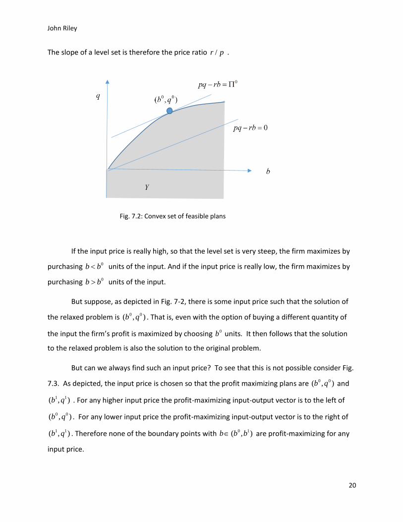
The slope of a level set is therefore the price ratio /r p .

If the input price is really high, so that the level set is very steep, the firm maximizes by

purchasing 0b b units of the input. And if the input price is really low, the firm maximizes by

purchasing 0b b units of the input.

But suppose, as depicted in Fig. 7-2, there is some input price such that the solution of

the relaxed problem is 0 0( , )b q . That is, even with the option of buying a different quantity of

the input the firm’s profit is maximized by choosing 0b units. It then follows that the solution

to the relaxed problem is also the solution to the original problem.

But can we always find such an input price? To see that this is not possible consider Fig.

7.3. As depicted, the input price is chosen so that the profit maximizing plans are 0 0( , )b q and

1 1( , )b q . For any higher input price the profit-maximizing input-output vector is to the left of

0 0( , )b q . For any lower input price the profit-maximizing input-output vector is to the right of

1 1( , )b q . Therefore none of the boundary points with 0 1( , )b b b are profit-maximizing for any

input price.

Fig. 7.2: Convex set of feasible plans

John Riley

21

The problem is that the set of feasible plans is not convex. While both 0 0( , )b q and

1 1( , )b q are feasible, none of the convex combinations are in the set of feasible plans.

However if Y is convex, it is intuitively clear from Fig. 7.2 that for any point 0 0( , )b q on

the boundary, there is a line through this point such that all the points in Y lie below this line.

Let

0 0 0pq rb pq rb

be the equation of this line. Then

0 0 0

( , ){ }

b q Ypq rb Max pq rb

The crucial observation is that if Y is convex, then for every input-output vector 0 0 0( , )y b q

on the boundary of Y there is a vector of prices ( , )p r for which 0y is profit-maximizing.

Therefore we can solve the constrained maximization by considering the relaxed maximization

problem.

Fig. 7.3: Profit-maximization

John Riley

22

In fact this is true, whether there as a single input b or a vector of inputs.

This result is summarized in the following proposition.

Proposition: Supporting prices

For a convex set X , Let {( , ) | ( ) 0, ( ) 0, 1,..., , }i iY b q f x q b g x i m x X be the set

of feasible plans.

For any 0b , the maximum feasible output 0q is the solution to the following maximization

problem.

0 0{ | ( ) 0, ( ) ( ) 0, 1,..., }i i ix X

q Max q f x q h x b g x i m

. (7.3)

If Y is convex (as is the case when f and , 1,...,ih i m are concave functions of x ) then

there is supporting price vector ( , )p r where 0p and 0r such that 0 0( , )b q is profit-

maximizing.

8. Constrained maximization

We now consider the following constrained maximization problem

0 0{ ( ) | ( ) ( ) 0, 1,..., }n i i i

xq Max f x h x b g x i m

(8.1)

From the supporting prices proposition, if the problem is concave (i.e. ( )f x and

( ), 1,...,ih x i m are concave functions of x ), and 0q is the solution to this maximization

problem, then there exists prices such that

0 0

1

{ | ( ) , ( ) , 1,..., }m

i i i ix X

i

pq rb Max pq rb f x q g x b i m

Since 0p , profit can be increased if ( )q f x . Therefore ( )f x q and we can rewrite the

maximization problem as follows:

John Riley

23

0 0

1

{ ( ) | ( ) , 1,..., }m

i i i ix X

i

pq rb Max pf x rb g x b i m

If 0ir , profit can be increased by decreasing ib if 0( )i ig x b . Then in such cases

0 0( )i i i irb rg x .

If 0ir this equality again holds. Therefore we can rewrite the maximization problem as

follows:

0 0

1

{ ( ) ( )}m

i ix X

i

pq rb Max pf x r g x

(8.2)

Define /i ir p . Then

0 0

1

{ ( ) ( )}m

i ix X

i

pq rb p Max f x g x

.

We have therefore shown that the solution to the constrained maximization problem must also

be the solution to an unconstrained maximization problem in which each of the inputs has a

“shadow price”.

The FOC for 0x to be a solution to this unconstrained maximization problem has

already been examined in section 4. There is a simple way of remembering these conditions.

Step 1: Write down each constraint as follows: ( ) ( ) 0i i ih x b g x .

Step 2: Write down the Lagrangian

1

( , ) ( ) ( )m

i i

i

L x f x h x

.

Step 3: Write down the gradient of this function

1

( , ) ( ) ( )m

ii

ij j j

hL fx x x

x x x

.

Step 4: FOC (from section 4):

John Riley

24

If 0 0jx then 0( , ) 0j

Lx

x

. If 0 0jx then 0( , ) 0

j

Lx

x

.

Example: Consumer choice

A consumer has utility function 1

( ) lnn

j j

j

U x x

. The price vector is 0p and her income

is I . She maximizes her utility subject to a her budget constraint, That is, she solves the

following problem.

0

1 1

{ ( ) ln | ( ) 0}n n

j j j jx

j j

Max U x x h x I p x

Since ln x is concave the utility function is concave as it is the sum of concave functions. The

constraint function ( )h x is also concave because it is the sum of linear (and hence concave)

functions. Thus if we can find 0x satisfying the FOC, it is a maximizer.

Suppose that 0 0x is a solution. Note first that since utility is increasing, the budget

will be satisfied with equality at the maximum 0

1

( )n

j j

j

p x I

. The Lagrangian is

1 1

ln ( )}n n

j j j j

j j

L x I p x

At 0x the FOC are

0

0( , ) 0

j

j

j j

Lx p

x x

, 1,...,j n .

Therefore

0

j j jp x , 1,...,j n . (8.3)

Summing over the commodities,

John Riley

25

0

1 1

n n

j j j

j j

p x I

.

Therefore 1

1 n

j

jI

.

Appealing to (8.3),

0

1

j j

j n

j jj

j

Ix

p p

.