Jolly-Seber models in MARK - phidot.org · Jolly-Seber models in MARK Carl James Schwarz, Simon Fraser University ... occasion i (the CJS models referred only to marked animals);

CHAPTER 12

Jolly-Seber models in MARK

Carl James Schwarz, Simon Fraser University

A. Neil Arnason, University of Manitoba

The original Jolly-Seber (JS) model (Jolly, 1965; Seber, 1965) was primarily interested in estimating

abundance. Since then, the focus of many mark-recapture experiments changed to estimating survival

rates (but not abundance) using the Cormack-Jolly-Seber (CJS)models (Cormack, 1964; Jolly, 1965; Seber,

1965) particularly with the publication of Lebreton et al. (1992). In previous chapters concerning analysis

of live encounter data,we have focussed exclusively on CJS models. In recent years,however, interest has

returned to estimating parameters related to abundance such as population growth (λi), recruitment

( fi), as well as abundance (Ni).∗

Much of the theory about estimating population growth, recruitment, and abundance can be found

in Williams et al. (2002).

12.1. Protocol

The protocol for JS experiments is very similar to that of CJS experiments. In each of K sampling

occasions, animals are captured. Unmarked animals are tagged with individually identifiable tags

and released. Previous marked animals have their tag numbers read and are again released.† The key

difference between JS and CJS experiments is the process by which unmarked animals are captured and

marked. In CJS experiments, no assumptions are made about how newly marked animals are obtained.

The subsequent process of recovering marked animals in CJS models is conditional upon the animal

being released alive at first encounter, and survival and catchability refer only to these marked animals.‡

In JS experiments, the process by which unmarked animals are newly captured to be marked and

released is crucial – the assumptions about this process allows the experimenter to estimate recruitment

and population sizes. In particular, it is assumed that unmarked animals in the population have the

same probability of capture as marked animals in the population, i.e., that newly captured unmarked

animals are a random sample of all unmarked animals in the population.

∗ One of the reasons for preferring estimation of population growth is that estimates of population growth are fairly robustagainst heterogeneity in catchability (Schwarz, 2001), and tag loss (Rotella and Hines, 2005).

† Losses on capture are possible at every sampling occasion and are ignored in the discussion that follows.‡ Of course, we hope that the survival of the marked subset of animals tells us something about the remaining unmarked animals

in the population at large.

© Cooch & White (2018) 02.05.2018

12.2. Data 12 - 2

This assumption of equal catchability for marked and

unmarked animals is needed to estimate abundance

or recruitment or population growth and is required

for the Pradel, Link-Barker, POPAN, and Burnham JS

formulations in MARK...

Other assumptions about the experiment are similar to those for the CJS model:

• Animals retain their tags throughout the experiment.∗

• Tags are read properly.

• Sampling is instantaneous.

• Survival probabilities are the same for all animals (marked and unmarked) between

each pair of sampling occasions (homogeneous survival).

• Catchablity is the same for all animals (marked and unmarked) at each sampling

occasion (homogeneous catchability). This is the most crucial assumption for JS

models.†

• The study area is constant. If the study area changes over time, then the population

size may change with the changing size of the study area.

There are generally two sources of non-closure in any particular study. Animals may leave the

population through death or permanently emigrate. Conversely, animals may enter the study area from

outside (immigration) or be recruited from within the study area (e.g. fish growing into the catchable

portion of the population). Specific tests for closure have been developed (e.g., Stanley and Burnham,

1999), but more often tests for closure are performed by fitting models with no apparent mortality

(ϕ � 1), or no apparent recruitment ( f � 0, λ � ϕ, or b � 0), or both and letting the AICc indicate the

appropriate weight for such simpler models.

12.2. Data

The basic unit of analysis is the capture history, a sequence of 0’s and 1’s that indicates when a particular

animal was seen in the experiment. The JS models in MARK use the LLLLL capture history format. For

example, the history (‘011010’) indicates that an animal was captured for the first time at sampling

occasion 2, was seen again at sampling occasion 3, not seen at sampling occasion 4, seen at sampling

occasion 5, and not seen after sampling time 5.‡ Either individual or grouped capture histories may be

used.

In many papers, the list of capture histories is too long to publish, and so a series of summary statistics

are commonly used (Table 12.1; see also the reduced and full m-array descriptions in Chapter 5). For

example, the history (011010) would contribute a count of 1 to n2, n3, n5, u2, m3, m5, R2, R3, R5, r2, r3,

and z3.

∗ Refer to Cowen and Schwarz (2006) for dealing with tag loss in JS experiments.† Refer to Pledger and Efford (1998) for details on dealing with heterogeneity in JS models.‡ Again losses on capture are ignored for now but are handled in the same way as elsewhere in MARK.

Chapter 12. Jolly-Seber models in MARK

12.3. Multiple formulations of the same process 12 - 3

Table 12.1: Summary statistics often used for JS experiments. Losses-on-capture are found as ni − Ri .

Statistics Definition

ni Number of animals captured at occasion i, both marked and unmarked.

ni � mi + ui .

ui Number of unmarked animals captured at occasion i.

mi Number of previously marked animals captured at occasion i.

Ri Number of animals released alive at occasion i+, i.e., just after sampling

occasion i.

ri Number of animals from Ri that are subsequently captured after occasion

i.

zi Number of animals seen before i, seen after occasion i, but not seen at

occasion i.

While these summary statistics form the sufficient statistics for the Jolly-Seber probability model,

their use has fallen out of favor in place of the raw histories used by MARK for two reasons. First,

the use of individual covariates will require the individual capture history vectors (see Chapter 2, and

Chapter 11).

Second, it is difficult to compute goodness-of-fit statistics (i.e., the RELEASE suite of tests; Chapter 5)

from the summary statistics.∗ If only summary statistics are available, it is possible to work ‘backwards’

and create a set of histories that will reproduce these summary statistics that can be used with MARK

to fit various models. One problem in using these pseudo-histories is that goodness-of-fit tests are

nonsensical – the goodness-of-fit tests require the full capture history of each animal.

12.3. Multiple formulations of the same process

There are a number of formulations used in MARK to estimate abundance and related parameters, e.g.,

the POPAN; the Link-Barker and Pradel-recruitment; and the Burnham JS and Pradel-λ formulations.

All of these models are slightly different parameterizations of the underlying population processes, and

all are (asymptotically) equivalent in that they should give the same estimates of abundance and related

parameters.

The two main differences among the various formulations are

1. the way in which they parameterize new entrants to the population

2. if estimation is conditional upon the animals actually seen in the study (refer to

Sanathanan 1972, 1977).

All of the formulations model the recapture of marked animals in the same way. In this section,

several of these models will be examined and contrasted.

∗ Indeed, if the summary statistics are used by themselves, the fully time dependent JS models will be ‘perfect’ fit to the summarystatistics regardless if the model overall is a good fit.


12.3.1. The Original Jolly-Seber formulation 12 - 4

12.3.1. The Original Jolly-Seber formulation

In the original JS formulation of Jolly (1965) and Seber (1965), the population process can be modeled as

shown in Figure 12.1. The parameters pi and ϕi are similar, but not identical to those in the CJS models.

The parameter pi is the probability of capture of both unmarked and marked animals that are alive at

occasion i (the CJS models referred only to marked animals); the parameter ϕi refers to the survival

probabilities of both marked and unmarked animals between occasions i and i + 1 (the CJS models

referred only to marked animals).

Figure 12.1: Original process model for JS experiments. pi represents the probability of capture at occasioni; ϕi represents the probability of an animal surviving between occasions i and i + 1; and Mi and Uirepresent the number of marked and unmarked animals alive at occasion i. Losses-on-capture are notmodeled here, but are easily included.

ϕ1 ϕ2 ϕ3 ϕ4

t1 → t2 → t3 → t4 → t5 . . .

↑ ↑ ↑ ↑ ↑

p1 p2 p3 p4 p5

M1 M2 M3 M4 M5

U1 U2 U3 U4 U5

The number of marked animals in the population just before occasion i + 1 is found as Mi+1 �

(Mi + ui)ϕi where ui is the number of newly unmarked animals captured and subsequently marked.

The number of net new entrants to the population was defined as

Bi � Ui+1 − ϕi(Ui − ui).

The Bi values refer to the net number of new entrants to the population between sampling occasions

i and i + 1. The reference to ‘net’ number of new entrants implies that animals that enter between two

sampling occasions but then die before being subject to capture at occasion i+1 are excluded.∗ As in the

CJS models, the term survival refers to apparent survival – permanent emigration is indistinguishable

and treated the same as mortality. Similarly, the term births refers to any new animals that enter the

study population regardless if in situ natural births or immigration from outside the study area.

The likelihood function consists of three parts. The first part models losses-on-capture using a simple

binomial distribution as in the CJS models. The second part models the recapture of marked animals in

exactly the same way as in the CJS model. Finally, the third part models the number of unmarked animals

captured at occasion i as a binomial function of the number of unmarked animals in the population, i.e.,

ui is Bin(Ui , pi).

The estimates of pi and ϕi are found in exactly the same way as in the CJS models. The estimated

unmarked population sizes were estimated as Ui � ui/pi . The estimated number of births was found by

substituting in the estimates in the previous definition and does not form part of the likelihood. Finally,

estimates of population size at each time point are found by adding the estimates of Ui and Mi .

∗ The term gross number of entrants would include these deaths prior to the next sampling occasion. Refer to Schwarz et al. (1993)for details on the estimation of these gross births.


12.3.2. POPAN formulation 12 - 5

12.3.2. POPAN formulation

Schwarz and Arnason (1996) adopted a slightly different parameterization, for a number of reasons:

• The parameters Bi never directly entered into the likelihood function. The number

of entrants must be non-negative, but it was difficult to enforce Bi ≥ 0 and negative

estimates of births were often obtained.

• Because the Bi did not appear in the likelihood, how could these be forced to be

equal across groups following the Lebreton et al. (1992) framework?

• How could death-only models (e.g., all Bi known to be zero) or birth-only models

(all ϕi=1) or closed models be obtained by constraining the likelihood function.

In their parameterization, first implemented in the computer package POPAN and now a sub-module

of MARK, they postulated the existence of a super-population consisting of all animals that would ever

be born to the population, and parameters bi which represented the probability that an animal from

this hypothetical super-population would enter the population between occasion i and i + 1 as shown

in Figure 12.2.∗

Figure 12.2: Process model for POPAN parameterization of JS experiments. pi represents the probability ofcapture at occasion i; ϕi represents the probability of an animal surviving between occasions i and i+1; andbi represents the probability that an animal from the super-population (N) would enter the populationbetween occasions i and i + 1 and survive to the next sampling occasion i + 1. Losses-on-capture areassumed not to happened, but are easily included.

b0 b1 b2 b3 b4 N

ϕ1 ϕ2 ϕ3 ϕ4

t1 → t2 → t3 → t4 → t5 . . .

↑ ↑ ↑ ↑ ↑

p1 p2 p3 p4 p5

Now the expected number of net new entrants is simply found as E[Bi] � Nbi . If B0 represents the

number of animals alive just prior to the first sampling occasion, then

N � B0 + B1 + B2 + · · · + BK−1

In other words, the total number of animals that ever are present in the study population. The

parameters bi are referred to as PENT (Probability of Entrance) probabilities in MARK. Notice that

b0+b1+ · · ·+bK−1 � 1; – this will have consequences later when the models are fitted using MARK. Even

though the number of new animals is not modeled in the process, modeling the entrance probabilities

and a super-population size is equivalent.

∗ The super-population approach was first described by Crosbie and Manly (1985) where distribution functions (e.g. a Weibulldistribution) was used to model survival time once an animal had entered the population. To our knowledge, there is no readilyavailable computer code for the Crosbie and Manly (1985) model.



Under this parametrization,

E[N1] � Nb0

E[N2] � E[N1]ϕ1 + Nb1

...

The probability ofany capture history can be expressedusing these parameters. Forexample,Pr[(01010)]

is found as:

Pr [(01010)] �[

b0

(

1 − p1

)

ϕ1 + b1

]

p2ϕ2

(

1 − p3

)

ϕ3p4

[

1 − ϕ4 + ϕ4

(

1 − p5

) ]

.

As in the CJS models, the fate of the animal after the last capture is unknown – either it died, or it

survived and was not seen at occasion 5. In a symmetrical fashion, the fate of the animal before the first

time it is captured is also unknown. Either it was present in the population prior to sampling occasion

1 and wasn’t seen at occasion 1 and survived to occasion 2, or it entered the study population between

sampling occasions 1 and 2 and survived to sampling occasion 2 where it was captured for the first

time. The likelihood function is again a multinomial function over all the observed capture histories.

Schwarz and Arnason (1996) showed that it could be factored into three parts:

L � Pr(

first capture)

× Pr(

subsequent recaptures)

× Pr(

loss on capture)

,

where the second and third components are identical to the CJS models. It turns out that similar to CJS

models,not all parameters are identifiable and only functions of parameters can be estimated in the fully

time-dependent model. The set of non-identifiable parameters is given in Table 12.2. In particular, the

final survival and catchability parameters are confounded (as in the CJS models), and symmetrically

the initial entrance and catchability are confounded. This impacts three other sets of parameters, in

particular N1 and NK cannot be cleanly estimated, nor can b1 and bK−1. If confounding takes place, the

estimated super-population number may be suspect, so some care must be taken in fitting appropriate

models. For example, models with equal catchability over sampling occasions make all parameters

identifiable.

This confounding implies that careful parameter counting may have to be done when fitting POPAN

models. The fully time-dependent model {pt ϕt bt } has K parameters for catchability, (K−1)parameters

for survival, K parameters for the PENTs, and 1 parameter for the super-population size for a total of

3K parameters. However, not all are identifiable and the PENTs must sum to one. Only the products

b0p1 and ϕK−1pK can be estimated, and one of the PENTs is not ‘free’ (as the sum must equal 1), leaving

(3K − 3) parameters that can be estimated for each group.

Furthermore, as indicated in Table 12.2 (top of the next page), the b1 and bK−1 parameters are affected

(the estimates reflect the combination of parameters as listed in the table) which further affect N1 and NK .

While the latter parameter combinations are ‘estimable’, they seldom represent anything biologically

useful. The actual number of parameters reported by MARK in the results browser should be checked

carefully.

Once estimates of p, ϕ, b, and N are obtained, the estimated number of births is obtained as Bi � N bi .

The estimated population sizes are obtained in an iterative fashion:

N1 � B0

N2 � N1ϕ1 + B1

...


12.3.3. Link-Barker and Pradel-recruitment formulations 12 - 7

Table 12.2: Confounded parameters in the POPAN parameterization in the fully time-dependent model. Inorder to resolve this confounding, the models must make assumptions about the initial (p1) and final (pK )catchabilities. For example, a model may assume that catchabilities are equal across all sampling occasions.

Function Interpretation

ϕK−1pK Final survival and catchability.

b0p1 Initial entrance and catchability.

b1 + b0(1 − p1)ϕ1 Entry between firstandsecondoccasions cannotbe cleanly estimated

because initial entrance probability cannot be estimated. MARK

(and other programs) will report an estimate for this complicated

function of parameters but it may not be biologically meaningful.

bK−1/ϕK−1 Entry prior to last sampling occasion cannot be cleanly estimated

because final survival probability cannot be estimated. MARK (and

other programs) will report an estimate for this complicated function

of parameters but it may not be biologically meaningful.

If losses on capture occur, they are removed before the population size at occasion i is propagated to

occasion i + 1.

The likelihood does not contain any terms for Bi or Ni – these are derived parameters and standard

errors for these estimates are found using the Delta method (see Appendix 2).

12.3.3. Link-Barker and Pradel-recruitment formulations

The Link-Barker (2005) and Pradel-recruitment∗ (1996) formulations are conceptually the same and

the process model is shown in Figure 12.3. The parameters for survival (ϕi) and catchability (pi) are

standard. The parameter fi is interpreted as a per capita recruitment probability , i.e., how many net new

animals per animal alive at occasion i enter the population between occasion i and i + 1?

Figure 12.3: Process model for Link-Barker and Pradel-recruitment parameterization of JS experiments. pirepresents the probability of capture at occasion i; ϕi represents the probability of an animal survivingbetween occasions i and i+1; and fi represents the net recruitment probability , i.e., the per capita numberof new animals that enter between occasions i and i+1 and survive to the next sampling occasion i+1 peranimal alive at occasion i. Losses-on-capture are assumed not to have happened, but are easily included.

f1 f2 f3 f4ϕ1 ϕ2 ϕ3 ϕ4

t1 → t2 → t3 → t4 → t5 . . .

↑ ↑ ↑ ↑ ↑

p1 p2 p3 p4 p5

∗ There are three different Pradel models and ‘-recruitment’ refers to the Pradel models parameterized using fi terms



Unlike the POPAN formulation, the Link-Barker formulation conditions upon an animal being seen

somewhere in the experiment. This eliminates the necessity of estimating the super-population size,

but also means that abundance cannot be directly estimated. Any probability of a history must be

normalized by the probability of being a non-zero history.

For example, Pr[(01010)|animal seen] is proportional to:

Pr [(01010)|animal seen] ∝[

(1 − p1)ϕ1 + f1]

/p1 × p2ϕ2

(

1 − p3

)

ϕ3p4

[

1 − ϕ4 + ϕ4

(

1 − p5

) ]

,

where the constant of proportionality is related to the probability of seeing an animal somewhere in

the experiment. As in the CJS models, the fate of the animal after the last capture is unknown – either

it died, or it survived and was not seen at occasion 5. In a symmetrical fashion, the fate of the animal

before the first time it is captured is also unknown – either it was present among animals seen in the

experiment at time 1, was not seen, and survived to time 2, or it entered between times 1 and 2. The

likelihood function is a multinomial function over all the observed capture histories conditional upon

an animal being seen somewhere in the experiment.

The implementation of the Link-Barker model differs from the Pradel-recruitment formulation in

a number of ways. First, Link-Barker partitioned the likelihood in a similar fashion to the POPAN

formulation which made it easier to implement in the Bayesian context of their paper. Second, Link-

Barker explicitly modeled the confounded parameters (but the MARK implementation leaves the

confounded parameters separate and it is the user’s responsibility to understand the confounding).

Third, losses on capture are handled differently between the two formulations and this affects the

interpretation of the recruitment parameters.

The Link-Barker model also differs from the POPAN formulation as there is no need to postulate the

existence of a super-population – the model is fit conditional upon the observed number of animals

in the experiment.∗ Section 12.3.5 outlines the equivalences between the Link-Barker parameters and

those of other formulations.

As in the POPAN formulation, the fully time-dependent Link-Barker and Pradel-recruitment models

have a number of parameter confoundings as listed in Table 12.3.

Table 12.3: Confounded parameters in the Link-Barker parameterization in the fully time-dependent model.In order to resolve this confounding, the models must make assumptions about the initial (p1) and final(pK ) catchabilities. For example, a model may assume that catchabilities are equal across all samplingoccasions.


ϕK−1pK Final survival and catchability

(ϕ1 + f1)/p1 Initial recruitment and survival

fK−1pK Final recruitmentandcatchability cannotbe cleanly estimated. MARK (and

other programs) will report an estimate for this complicated function of

parameters but it may not be biologically meaningful.

∗ The implementation of Schwarz and Arnason (1996) in the POPAN package also estimates parameters conditional upon beingseen, and then adds another step to estimate the super-population size.


12.3.4. Burnham JS and Pradel-λ formulations 12 - 9

On the surface, the fully time-dependent model {pt ϕt ft} has K catchability parameters, K−1 survival

parameters, and K − 1 recruitment parameters for a total of (3K − 2) parameters. However, only the

productϕK−1pK and the ratio ( f1/p1) can be estimated, leaving a net of (3K−4)parameters. The estimate

for fK−1 estimates are functions of other parameters as shown in Table 12.3.

The abundance at each sampling occasion and the absolute number of new entrants cannot be

estimated even as derived parameters because of the conditioning upon animals seen at least once

during the experiment.

12.3.4. Burnham JS and Pradel-λ formulations

The final formulations to be considered in this chapter model new entrants to the population indirectly

by modeling the rate of population growth (λ) between each interval where population growth is the

net effect of survival and recruitment. If ϕi is the decrease in the population per member alive at time i,

and fi is the increase in the population per member alive at time i, then the sum of their contributions

is the net population growth:

λi � Ni+1/Ni � ϕi + fi

. These formulations were developed by Burnham (1991) and Pradel (1996).

The key difference between the two parameterizations is that the Pradel-λ approach is conditional

upon animals being seen during the study, while the Burnham JS formulation is not. Therefore, the

Burnham Jolly-Seber formulation also includes a parameter for the population size at the start of the

experiment. This enables the estimation of the population size at each subsequent time point.

However, in practice, it is often difficult to get the Burnham-JS model to convergence during the

numerical maximization of the likelihood. Although the implementation of this model has been

thoroughly checked and found to be correct, MARK has some difficulty obtaining numerical solutions

for the parameters because of the penalty constraints required to keep the parameters consistent with

each other.∗ For this reason, only the Pradel-λ formulation will be discussed further in this section

(and treated in depth in Chapter 13). The process model is shown in Figure 12.4. The parameters for

survival (ϕi) and catchability (pi) are standard. The parameterλi is interpreted as the ratio of successive

population abundances.

Figure 12.4: Process model for Burnham and Pradel-λ parameterization of JS experiments. pi represents theprobability of capture at occasion i; ϕi represents the probability of an animal surviving between occasionsi and i + 1; and λi represents the rate of population change. The population size at time 1, N1 is usedby the Burnham formulation, but not by the Pradel-λ formulation. Losses-on-capture are assumed not tohappened, but are easily included.

ϕ1 ϕ2 ϕ3 ϕ4

λ1 λ2 λ3 λ4

t1 → t2 → t3 → t4 → t5 . . .

↑ ↑ ↑ ↑ ↑

p1 p2 p3 p4 p5

N1

∗ This convergence problem disappears for some models if simulated annealing is used for the numerical optimization. – J. Laake& E. G. Cooch, pers. obs.


12.3.4. Burnham JS and Pradel-λ formulations 12 - 10

Unlike the POPAN and Burnham formulations, the Pradel-λ formulation conditions upon an animal

being seen somewhere in the experiment. This eliminates the necessity of estimating the population

sizes at any sampling occasion. But, the probability of a history must now be normalized by the

probability of being a non-zero history. For example, Pr[(01010)|animal seen] is proportional to:

Pr [(01010)|animal seen] ∝[

λ1 − p1ϕ1

]

× p2ϕ2

(

1 − p3

)

ϕ3p4

[

1 − ϕ4 + ϕ4

(

1 − p5

) ]

,

where the constant of proportionality is related to the probability of seeing an animal somewhere in

the experiment.

As in the CJS models, the fate of the animal after the last capture is unknown – either it died, or it

survived and was not seen at occasion 5. In a symmetrical fashion, the fate of the animal before the first

time it is captured is also unknown – either it was present at the initial sampling occasion and not seen,

or was part of the population growth (over and above survival from the first sampling occasion). The

likelihood function is a multinomial function over all the observed capture histories conditional upon

an animal being seen somewhere in the experiment.

Section 12.3.5 outlines the equivalences between the Pradel-λ parameters and those of other formu-

lations.

As in the POPAN formulation, the fully time-dependent Pradel-λ formulation has a number of pa-

rameter confoundings as listed in Table 12.4. On the surface, the fully time-dependent model {pt , ϕt , λt }

has K catchability parameters, (K − 1) survival parameters, and (K − 1) growth parameters for a total

of 3K − 2 parameters. However, only the product ϕK−1pK and the function λ1 − ϕ1p1 can be estimated,

leaving a net of (3K − 4) parameters. Furthermore, the estimate for λK−1 estimates a function of other

parameters and may not be interpretable.

The abundance at each sampling occasion and the absolute number of new entrants cannot be

estimated even as derived parameters because of the conditioning upon animals seen at least once

during the experiment.

Table 12.4: Confounded parameters in the Pradel-λ parameterization in the fully time-dependent model. Inorder to resolve this confounding, the models must make assumptions about the initial (p1) and final (pK )catchabilities. For example, a model may assume that catchabilities are equal across all sampling occasions.


ϕK−1pK Final survival and catchability

λ1 − ϕ1p1 Initial growth and survival

λK−1pK Final recruitmentandcatchability cannotbe cleanly estimated. MARK (and

other programs) will report an estimate for this complicated function of

parameters but it may not be biologically meaningful.

Because population growth (λ) is a function both of survival and recruitment (i.e., λi � ϕi + fi),

the modeler should be careful about fitting simpler models that restrict population growth but leave

survival time-dependent. For example the model { pt , ϕt , λ•} would imply that recruitment varies in

a time dependent fashion to exactly balance changes in survival to keep population growth constant.

This may not be a sensible biological model.


12.3.5. Choosing among the formulations 12 - 11

Another potential problem with the Pradel-λ model is that no constraints are imposed in MARK

that population growth must exceed the estimated survival probability. Consequently (as seen in the

examples that follow), it is possible to get estimated survival probabilities of 80% while the estimated

population growth rate is only 70%. This logically cannot happen, and is often an indication that

recruitment did not occur in that interval – the illogical estimates are artifacts of the estimation process.

Under these circumstances,models that separate recruitment from population growth may be preferred.

12.3.5. Choosing among the formulations

All of the formulations use the same input file in the same format. Which JS formulation should be used

for a particular experiment? There are two considerations.

First, only certain of the formulations can be used in MARK if losses-on-capture occur in the

experiment.

Secondly, and more importantly, different formulations give you different types of information and

can be used to test different hypotheses. All of the formulations should give the same estimates of

survival and catchability, as all formulations estimate these from recaptures of previously marked

animals using a CJS likelihood component. Even though all the models give different types of estimates

for growth or recruitment or births, it is always possible to transform the estimates from one type to

another by simple transformation and the standard errors can be found using the Delta method.

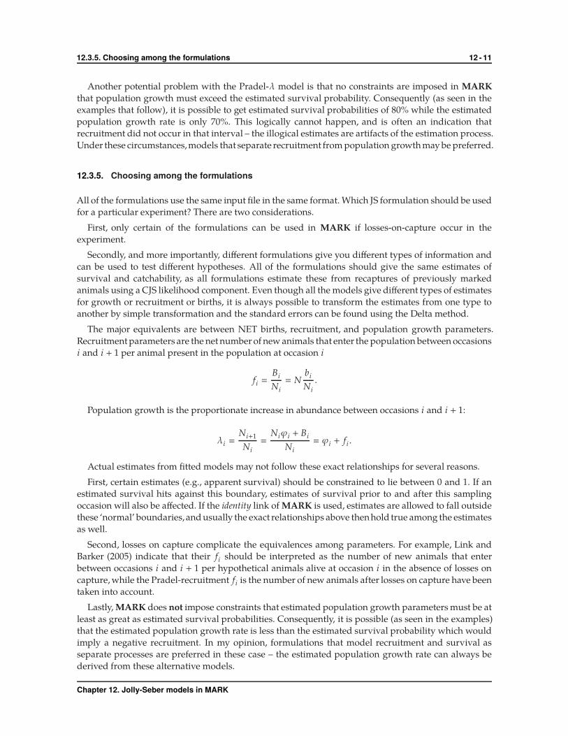
The major equivalents are between NET births, recruitment, and population growth parameters.

Recruitment parameters are the net number of new animals that enter the population between occasions

i and i + 1 per animal present in the population at occasion i

fi �Bi

Ni

� Nbi

Ni

.

Population growth is the proportionate increase in abundance between occasions i and i + 1:

λi �Ni+1

Ni

�

Niϕi + Bi

Ni

� ϕi + fi .

Actual estimates from fitted models may not follow these exact relationships for several reasons.

First, certain estimates (e.g., apparent survival) should be constrained to lie between 0 and 1. If an

estimated survival hits against this boundary, estimates of survival prior to and after this sampling

occasion will also be affected. If the identity link of MARK is used, estimates are allowed to fall outside

these ‘normal’ boundaries,and usually the exact relationships above thenhold true among the estimates

as well.

Second, losses on capture complicate the equivalences among parameters. For example, Link and

Barker (2005) indicate that their fi should be interpreted as the number of new animals that enter

between occasions i and i + 1 per hypothetical animals alive at occasion i in the absence of losses on

capture, while the Pradel-recruitment fi is the number of new animals after losses on capture have been

taken into account.

Lastly, MARK does not impose constraints that estimated population growth parameters must be at

least as great as estimated survival probabilities. Consequently, it is possible (as seen in the examples)

that the estimated population growth rate is less than the estimated survival probability which would

imply a negative recruitment. In my opinion, formulations that model recruitment and survival as

separate processes are preferred in these case – the estimated population growth rate can always be

derived from these alternative models.


12.3.6. Interesting tidbits 12 - 12

It cannot be emphasized too strongly, that all of the formulations require the same careful attention

to study design – in particular the study area must remain a consistent size, and the probability of

capturing an unmarked individual must be the same as a marked individual at each sampling occasion.

A Cormack-Jolly-Seber experiment where marked animals are captured and released haphazardly,

should not be then analyzed using any of the formulations of the Jolly-Seber model discussed in this

chapter.

Table 12.5: Summary of criteria to choose among the different JS formulations

losses on estimates available for

formulation capture abundance net births recruitment λ

POPAN yes yes yes no no

Link-Barker yes no no yes yes

Pradel-recruitment no no no yes yes

Burnham JS yes yes yes no yes

Pradel-λ yes no no no yes

• The implementation of Burnham’s JS model in MARK often does not converge, and is not

recommended (although convergence problems may be minimized for some models if simulated

annealing is used for the numerical optimization. - J. Laake & E. G. Cooch, pers. obs.)

• The standalone package of POPAN will estimate recruitment, and population growth as derived

parameters

12.3.6. Interesting tidbits

There have been a number of queries in the MARK forum (http://www.phidot.org/forum) about the

use of POPAN and other models to estimate abundance. This section will try to answer some of these

queries in more detail.

Deviance of 0 in POPAN

The following query was received in the MARK forum (http://www.phidot.org/forum, 2006-04-07)

which asked:

‘I read on one of the other posts that getting a deviance of zero was possible using the robust design

model because the saturated model hadn’t been computed yet and some constants were left out for

faster computation. Is something along these lines at play in POPAN also because when I run a

particular set of data, I get a deviance of zero?’

The deviance of models is often computed as the negative of twice the difference in the log-likelihood

between the current model and a ‘saturated’ model. The usual saturated model in CJS and other models

that condition upon an animal’s first capture, is to have a separate probability for each observed history,

i.e., if ω is a capture history (e.g., ‘010011’) then the Pr(ω) under the saturated model is found as

Pr(ω) �nω

nobswhere nω is the number of animals with capture history ω, and nobs is the total number of

animals observed.


12.4. Example 1 – estimating the number of spawning salmon 12 - 13

In such cases, the log-likelihood of the saturated model (ignoring constants) is then

∑

nω log(

pω)

�

∑

nω log( nω

nobs

)

.

However, this doesn’t work for models where abundance is estimated because you need to include

the animals with history (‘000000....’), i.e., those animals not observed. This can only be computed if the

population size is estimated which cannot be estimated under the saturated model. Hence a ‘deviance’

cannot be directly computed.

However, the likelihood can be portioned as shown earlier into components representing the proba-

bility of first capture, the probability of subsequent recapture given the animal has been captured, and

the probability of losses-on-capture given that an animal is captured. Schwarz and Arnason (1996) and

Link and Barker (2005) showed that the first component is essentially non-informative about the capture,

survival, and loss-on-capture rates.

This suggests that an approximate deviance could be computed using only the latter two components,

i.e., by conditioning upon animals that are seen at least once in the experiment. The difference between

the two likelihoods would be based only on the part representing animals seen at least once.

In practice, we would suggest that you compute a deviance based on conditioning on the observed

animals. The easiest way is to use the Link-Barker model (which doesn’t estimate abundance) but is

‘equivalent’ to the POPAN model. So if you fit a {pt ϕt bt } model in POPAN look at the deviance of the

{pt ϕt ft } model in Link-Barker formulation. This could be used to estimate a variance-inflation factor

to adjust reported standard errors.

12.4. Example 1 – estimating the number of spawning salmon

After spending several years at sea, coho salmon (Oncorhynchus kisutch) return to spawn in the Chase

River, British Columbia. The normal life cycle of coho salmon is to return at age 3 as adults to spawn

and die. But, some precocious males return earlier at age 2 to spawn and die. One question of interest

is if the distribution of salmon that return to spawn at different parts in the spawning period the same

for regular adult and precocious males?

As fish return to the Chase River, they are captured using electrofishing gear. If they are unmarked

they are given a unique tag number and released. If they were previously marked, the tag number is

read. The experiment took place over a 10 week period in 1989, but the data from weeks 1 and 2, and

weeks 9 and 10 were pooled and labeled as weeks 1.5 and 9.5. Approximately the same amount of effort

was expended in each week of sampling. More details of this experiment are found in Schwarz et al.

(1993).

The datafile is given in the chase_both.inp file, and a portion of it is reproduced in Figure 12.5 (top

of the next page). This study has two groups, the regular adult males and the precocious males (called

jacks). Notice that a separate capture history is used for each tagged fish – unfortunately, this implies

that the residual plots and deviance plots in MARK cannot be used to assess goodness of fit.



Figure 12.5: Portion of the data for the Chase 1989 experiment

/* Estimating salmon numbers returning to spawn in Chase River 1989 */

/* These are the male salmon with two groups. */

/* Group1 = adults . group2=jacks */

/* Survey conducted over 10 weeks. Weeks 1 & 2 pooled. weeks 9 & 10 pooled */

11000000 -1 0 ; /* tagnum=1 */

10000000 0 1 ; /* tagnum=3 */

10000000 0 1 ; /* tagnum=4 */

10000000 0 1 ; /* tagnum=6 */

11000000 0 1 ; /* tagnum=8 */

10110000 0 1 ; /* tagnum=9 */

10000000 0 1 ; /* tagnum=10 */

10000000 1 0 ; /* tagnum=11 */

... additional histories follow ....

Summary statistics for this experiment are presented in Table 12.6.

Table 12.6: Summary statistics for the Chase 1989 experiment

statistics for adults statistics for jacks

ti ni mi ui Ri ri zi ti ni mi ui Ri ri zi

1.5 37 0 37 37 12 0 1.5 67 0 67 62 21 0

3.0 22 6 16 21 13 6 3.0 28 9 19 25 7 12

4.0 52 7 45 41 19 12 4.0 46 6 40 44 9 13

5.0 56 17 39 54 26 14 5.0 47 12 35 45 5 10

6.0 46 26 20 38 8 14 6.0 25 9 16 24 3 6

7.0 28 16 12 20 2 6 7.0 16 6 10 12 1 3

8.0 22 3 19 16 2 5 8.0 7 1 6 5 1 3

9.5 10 7 3 0 0 0 9.5 7 4 3 0 0 0

Because ni > Ri for some sampling occasions, this indicates that some losses-on-capture occurred.

For example, there was one adult loss-on-capture in week 3; 11 adults lost in week 4, etc.


The POPAN super-population is a natural way to think of this experiment – a pool of fish is returning to

spawn. During each week, a certain fraction of these returning fish decide to enter the spawning areas.

Let us begin by fitting a model only to the regular adults (use the input file chase_adult.inp), i.e.,

to the first group. Later models will be fit to both groups (and will require the chase_both.inp file).

Launch MARK. Select the POPAN data type, enter the number of sampling occasions and the number

of attribute groups, as shown at the top of the next page.



Don’t forget to set the intervals between sampling occasions. As weeks (1 and 2) were pooled and

labeled as week 1.5, the interval between the first and second sampling occasion is 1.5 weeks. Similarly

weeks (9 and 10) were pooled and so the last interval is also longer.

Start by fitting a fully-time dependent model {pt , ϕt bt } (using an obvious notation extension from

CJS models). In this model there are 8 sampling occasions which give rise to 8 capture probabilities, 7

apparent survival probabilities, 8 probability of entry probabilities, and 1 super-population parameter.

Note that MARK does not allow the user to specify the parameter b0 (the proportion of the population

available just before the first sampling occasion) and so only presents 7 PENT parameters in the PIM

and output corresponding to b1 , . . . , b7.∗

∗ In the stand alone POPAN package, the user has access to all of the PENT’s.



Note that unlike the CJS models, we assume a single set of survival and catchability parameters, regardless

of when previously captured. The super-population size has its own parameter.

Because b0 + b1 + · · · + bK−1 � 1, a special link-function must be specified for the PENT parameters.

This is done using the ‘Parameter specific link function’ radio button:

The sin or logit or any of the other link functions can be used for the p and ϕ parameters. In order

to specify that a set of parameters must sum to 1, the Multinomial Logit link function (called Mlogit in

MARK) must be used. If there are several groups, each set of PENTs must independently sum to 1, so

MARK provides several sets of MLogit link functions. As there is only one group, the MLogit(1) link-

function is used for the PENTs. It is possible to specify that some of the PENTs are zero if, for example,

the experimenter knew that no new animals entered the study population during this interval.



Also notice, that a log or identity link should be used for the super-population size as it is not restricted

to lie between 0 and 1:

Now run MARK. If we look at the REAL estimates, we must keep in mind that not all parameters

are identifiable:

In particular, the final survival and catchability are confounded as in the CJS model. The initial

entrance and catchability parameters are also confounded (only the product b0p1 can be estimated)

– however, MARK does not report b0 so the first PENT reported here refers to b1 which cannot be

estimated separately (refer to Table 12.2). This non-identifiability can often be recognized by the large

standard errors for certain estimates, or by estimates tending to the value 1.0. Also notice, that because

the intervals are unequal size, the survival probabilities are given on a per week basis, so that the survival

probability for the initial 1.5 week interval is found as 0.571.5� 0.43.



The estimates of population size and net births are found under the derived parameter section:

Again, not all parameters are identifiable. The derived parameters also include estimates of gross births

– these are explained in more detail in Schwarz et al. (1993).

Goodness-of-fit can be assessed using the RELEASE suite as in CJS models (see Chapter 5 for details

on RELEASE). The results are shown below.

There is some evidence of potential lack-of-fit as indicated by Test2 in component C3, but a detailed

investigation of that table shows it is not serious. Unfortunately, because individual capture histories

were used, residual plots are not useful.

Because ofparameter confounding, it is important to count the actualnumberof estimable parameters.

On the surface there are 24 parameters composedof8 capture parameters,7 survivalparameters,8 PENT

parameters and 1 super-population parameter. However, the PENTs must sum to 1, and Table 12.2



indicates that two parameters are lost to confounding which leaves a net of 21 actual identifiable

parameters. Check that the results browser shows 21 parameters for this model.

The original sampling experiment has approximately equal effort at all sampling occasions. Perhaps

a model with constant catchability over time is suitable, i.e., model {p· ϕt bt }. This model is specified

in the PIM in the usual fashion:

None of the other PIM’s need to be respecified. The model is run, and again the parameter specific

link functions must be specified for the PENTs (use the MLogit(1) link function) and for the super-

population size (use the log link function):

Now all parameters are identifiable (shown below):

The results show b1 � 0.044, b2 � 0.33, etc. These are interpreted as 4.4% of adult returning salmon

return between weeks 1.5 and 3; about 33% of adult returning salmon return to spawn between weeks



4 and 5, etc. The value of b0 � 0.352 is obtained by subtraction (b0 � 1 − b1 − b2 − · · · − bK−1). This is

interpreted as 35% of adults returning salmon has returned to spawn before sampling began in week

1.5.

The total number of salmon returning to spawn (the super-population) is estimated to be N � 332

(SE=29) fish. The derived birth parameters are found as Bi � N bi . For example, B1 � N b1 � (332 ×

0.044) � 14.9. This is interpreted as about 15 adult fish returned to spawn between weeks 1.5 and 3.

B0 � N b0 � (332 × 0.352) � 117 fish are estimated to be present before the first sampling occasion.

The derived estimates of population size are found iteratively and must account for losses-on-capture

and the unequal time intervals (which affects the survival terms).

N1 � B0 � 117.03.

N2 � (N1 − loss1 )ϕ1.51 + B1 � (117.03 − 0)0.5841.5

+ 14.92 � 67.2.

N3 � (N2 − loss2 )ϕ1.02 + B2 � (67.2 − 1)0.9261.0

+ 110.39 � 171.72

...

The number of identifiable parameters for this model is 16 composed of 1 capture parameters, 7

survival parameters, 8 PENT parameters and 1 super-population parameter less the restriction that the

PENTs must sum to 1. The number of parameters reported in the browser may have to be manually

adjusted to indicate the correct number of parameters.

Another sub-model can also be fit where the apparent survival probability (per unit time) is constant

over all intervals, i.e., model {p· ϕ· bt }. It is fit in the same fashion by adjusting the PIMs:

This model would have 10 parameters composed of 1 capture parameter, 1 survival parameter, 8

PENT parameters, and 1 super-population parameters with 1 restriction that the PENTs sum to 1.

The final results table (after making sure that the number of parameters is correct):

shows not much support for this final model. If model averaging is to be used, some care must be taken

as not all parameters are identifiable in all models. For example, most models with a pt structure, will

be unable to estimate abundance at the first (N1) or last (NK) sampling occasion; nor can recruitment

be estimated for the first (b1, or B1) or last (bK−1 or BK−1) interval.

Other models could be fit, e.g., an equal fraction of the super-population returns to spawn in each



week, but in this example is highly unlikely biologically and was not fit.

Now let us return to the real question of interest – do jacks and adults have the same return pattern?

This is now a two group problem and is handled in a similar fashion to the ordinary CJS model.

Start a new project,using chase_both.inp, and this time specify two groups (regular adults and jacks)

rather than a single group. Also specify the names of the two groups.

Now each parameter can vary over sampling occasions (intervals) and/or groups. The full model fit

will be specified by a triplet of specifications.

In the previous example, a model with equal catchability over sampling occasions was tenable, but

adults and jacks may have different catchabilities. Survival probabilities varied by time, so perhaps start

with a fully time- and group-dependent model for ϕ. Also start with a full group and time dependence

for the PENTs. This would correspond to model {pg ϕg∗t bg∗t } with the following PIMs.

The two PIMs for the super-population size of the adults and jacks (respectively) are not shown.

Request that MARK fit this model. As before, we must indicate to MARK that the PENTs sum to 1,

for each group using the parameter specific link functions.



There are a total of 8 sampling occasions, 8 PENTs per group, but MARK only shows the last seven

(b0 for each group is implicitly assumed). Use the MLogit(1) link function for the first seven PENTs

(belonging to group 1) and the MLogit(2) link function for the last seven PENTs (belonging to group 2).

Notice that only 30 parameters are displayed per window, so the ‘More’ button must be used to scroll

to the next page:

Don’t forget to specify that the two super-population parameters should have the identity or log link

function.

Run the model and add it to the results browser. Then, run and fit the models {pg ϕt bg∗t } and and

{pg ϕt bt }.∗

∗ The option to ‘Initial → Copy 1 PIM to another PIM’ is helpful here.



Count parameters carefully. All of the models have a simple structure for the p’s so there is no

problem with confounding. The model {pg ϕt bg∗t } has 2 catchability parameters, 7 survival parameters,

16 PENTs, and 2 super-population sizes. However, each set of PENTs must sum to 1, leaving 25 free

parameters. The model {pg ϕt bt } has 2 catchability parameters, 7 survival parameters, 8 PENTs (but

these must sum to 1), and 2 super-population parameters for a total of 18 parameters. The model

{pg ϕg∗t bg∗t } has 2 catchability parameters, 14 survival parameters, 18 PENTs (but each of the two

groups of PENTs must sum to 1), and 2 super-population sizes for a total of 32 parameters.

The final results window looks like (after adjusting for the number of parameters)

The final models of interest are a comparison between model {pg ϕt bg∗t } and {pg ϕt bt } (why?). The

∆AICc shows very little support for the model where the jacks enter in the same distribution as the

adults. In particular, examine the estimates of the PENTs for the {pg ϕt bg∗t } model:

Recall that even though there are 8 PENT parameters per group that MARK does not let you specify

the b0 parameter in the PIMS – this value is obtained by subtraction from 1. Further manipulations can

be done by copying the real parameter values to an Excel spreadsheet:

You will find that about 34% (1 − 0.033 − 0.326 − . . . − 0.000) of adults were in the stream prior to the

first sampling occasion, while about 69% (1 − 0.000 − 0.227 − 0.036 − . . . − 0.000) of jacks were in the

stream prior to the first sampling occasion. So it appears that precocious males tend to return earlier

(for this stream and year) than regular adults.



In this example, it is vitally important that catchability be approximately constant across all sampling

occasions so that a model with pg could be fit; any model where catchability varied across time (a pt

or pg∗t model) would have the first PENT parameter hopelessly confounded with the first catchability

parameter and in many cases, makes it difficult if not impossible to do sensible model comparisons.

This again illustrates the need for careful study design with JS models.

begin sidebar

The multinomial logit link and the POPAN model

In situations where you want to constrain estimates from a set of 2 or more parameters to sum to 1,

you might use the multinomial logit link (MLogit), which was introduced in some detail in Chapter

10 with respect to multi-state models (where the transitions from a given stratum must logically sum

to 1.0).

While specifying the MLogit link in MARK is straightforward, you need to be somewhat careful.

Consider the following set of parameters in a PIM for the probability of entry (pent) in a POPAN

model:

61 62 63 64 65 66 67 68 69 70

The parameter-specific link would be selected in the ‘Setup Numerical Estimation Run’ window,

and the MLogit(1) link would be applied to parameters 61 → 70 to force these 10 estimates to sum to

≤ 1. But suppose that you wanted to force all of the 10 entry probabilities to be the same, and have the

sum of all 10 be ≤ 1? You might be tempted to specify a PIM such as

61 61 61 61 61 61 61 61 61 61

(i.e., simply use the same index value for all the parameters in the PIM), but that would be incorrect.

Changing the PIM and selecting the MLogit link for parameter 61 would result in parameter 61 alone

summing to ≤ 1 (i.e., just like a logit link), but would not force the sum of the 10 values of parameter

61 to sum to ≤ 1.

To implement the proposed model, the PIM should not be changed from the top example (i.e., it

should maintain the indexing from 61 → 70), and the design matrix should be used to force the same

estimate for parameters 61 → 70:

Parameter Design Matrix

61 1

62 1

63 1

64 1

65 1

66 1

67 1

68 1

69 1

70 1

Then the MLogit(1) link should be specified for the 10 parameters 61 → 70. The result is that now all

10 parameters have the same value, and 10 times this value is le1.

Another example – suppose you wanted parameters 61 and 62 to be the same value, 63 to 66 the

same, 67 and 68 the same, and 69 and 70 the same, but the sum over all parameters to be ≤ 1. Again

you would use the PIM

61 62 63 64 65 66 67 68 69 70

but again use the design matrix to implement the constraints. The following design matrix is one

example that would produce such a set of constraints.



Parameter Design Matrix

61 1 1 0 0

62 1 1 0 0

63 1 0 1 0

64 1 0 1 0

65 1 0 1 0

66 1 0 1 0

67 1 0 0 1

68 1 0 0 1

69 1 0 0 0

70 1 0 0 0

The key point with these examples is that the PIM cannot be used to constrain parameters if you

want the entire set of parameters to sum to ≤ 1. Rather, the design matrix has to be used to make the

constraints, with each of the entries in the PIM given the same MLogit(x) link. Further examples of

the MLogit link are discussed in Chapter 10.

end sidebar


The Link-Barker or Pradel-recruitment formulation can be conveniently obtained by switching data

types from any of the JS formulations. We will illustrate the use of the Link-Barker formulation; that for

the Pradel-recruitment is similar, but in this case cannot be used because of losses-on-capture.

Let us begin with a time dependent model for all parameters, i.e., {pt ϕt ft }. The number of groups

and sampling intervals would have been entered as seen in the POPAN formulation. The survival and

catchability PIMs mimic those for the POPAN formulation.

In the Link-Barker formulation, there are (K − 1) � 7 recruitment parameters with a standard PIM:

Because the population recruitment value is not limited to lie between 0 and 1 (for example, the

recruitment value could exceed 1), the ‘Parameter Specific Link’ functions should be specified when

models are run:∗

∗ An undocumented feature of MARK is that it will use the log link for the recruitment parameter if you specify a logit or sinlink in the radio buttons.



Any of the link functions can be used for the catchability and survival parameters (although the logit

and sin link are most common), but either the log or the identity link function should be used for the

population recruitment parameters. There are no restrictions that the recruitment parameters sum to 1

over experiment so the Mlogit link should not be used.

Run the model and append it to the browser.

As in the POPAN formulation, both the fully time-dependent Link-Barker and Pradel-recruitment

formulations suffer from confounding. If you examine the β parameter estimates, and the estimated SE

(below), there are several clues that confounding has taken place:



As in the POPAN formulation, survival in the last interval and catchability at the last sampling

occasion are confounded. The corresponding βparameters are very large on the logit scale withstandard

errors that are either zero or very large. Similarly, p1 cannot be estimated and its β standard error is very

large.

Finally, because the first and last catchabilities cannot be estimated, neither can ‘population size’

(despite population size not being explicitly in the model) and so the recruitment parameter (the fi

values) based on occasion 1 ( f1) or terminating with occasion K ( fK−1) cannot be estimated either. We

notice that the standard errors for these recruitment parameters are nonsensical.

The user must be very careful to count parameters carefully and to see if MARK has detected the

correct number of parameters. There are 8 sampling occasions. The fully time-dependent model has, on

the surface, 8 capture parameters, 7 survival parameters, and 7 recruitment recruitment parameters for

a total of 22 parameters. However, as shown in Table 12.3, there are two parameters lost to confounding

which gives a total of 20 parameters that can be estimated. The number of parameters reported in the

results browser may have to be modified manually.

As in the POPAN formulation, models where constraints are placed on the initial and final catchabil-

ities can resolve this confounding. Because roughly the same effort was used in all sampling occasions,

the model {p• , ϕt , ft } seems appropriate.

Adjust the PIM for the recapture probabilities to be constant over time, re-run the model (don’t forget

to use the ‘Parameter Specific Link’ function option),∗ and append the results to the browser. Let’s

look at the parameter estimates (top of the next page). The number of parameters that can be estimated

is now 15 being composed of 1 capture parameter, 7 survival parameters, and 7 recruitment parameters.

If you compare the estimates of p and ϕ between the Link-Barker formulation and the POPAN

formulation they are identical (except for rounding errors). Note that because of unequal time intervals,

estimates of ϕi are on a per-unit basis. The actual survival in the first and last interval must be obtained

by raising the reported ϕ’s to the 1.5th power (corresponding to the 1.5 week interval).

∗ CAUTION: When we ran this model with the logit link for the ϕ’s, one ϕ converged to a value of 1; we would recommend thatthe sin link be used.



The PENTs from POPAN and the f ’s from the Link-Barker are not directly comparable. However, the

following equivalents are noted:

( f LB1 )1.5 � 0.2521.5

� 0.127 �

BPOPAN1

NPOPAN1

�14.92

117.034

f LB2 � 1.644 �

BPOPAN2

NPOPAN2

�110.39

67.20

f LB3 � 0.211 �

BPOPAN3

NPOPAN3

�36.77

171.72

. . .

Similarly, estimates of population growth are also equivalent:

( f LB1 )

1.5+ (ϕ

LB1 )

1.5� 0.5831.5

+ 0.2521.5� 0.571 �

NPOPAN2

NPOPAN1

�

67.20

117.03� 0.574

f LB2 + ϕLB

2 � 1.644 + 0.928 � 2.57 �

NPOPAN3

NPOPAN2

�171.72

67.20� 2.55

. . .

If you examine the results browser (after any changes for the actual number of parameters that are

estimated):

you will also see that the ∆AICc values between these two models matches very closely with the


12.4.3. Burnham Jolly-Seber and Pradel-λ formulations 12 - 29

difference in the POPAN formulation. The differences in ∆AICc between the two formulation are

artifacts of the different number of parameters estimated and the small sample correction applied to

the AIC. If the actual AIC values from the two formulations are compared, the difference in AIC are

nearly identical because the two formulations are simply re-parameterizations of the same models for

modeling the marked animals and only differ in estimating the super-population size.

As Sanathanan (1972, 1977) showed, the conditional approach of Link and Barker (2005) is asymp-

totically equivalent to the full likelihood approach of Schwarz and Arnason (1996). For example, in

the table shown below, the log-likelihood and AIC (before small sample corrections are applied) were

extracted from the model outputs. The differences in the log-likelihoods and the AIC among the models

in different formulations are nearly the same.

POPAN formulation Link-Barker formulation

Model −2 × logL # parms AIC Model −2 × logL # parms AIC

{p· , ϕt , bt } 489.94 16 521.94 {p· , ϕt , ft} 1176.74 15 1206.74

{p· , ϕ· , bt} 507.25 10 527.25 {p· , ϕ· , ft} 1193.99 9 1211.99

{pt , ϕt , bt} 486.80 21 528.80 {pt , ϕt , ft} 1173.69 20 1213.69

The two group case can be fit in a similar fashion as seen in the POPAN example. However, it

is not clear exactly which models should be compared because the fi parameters in the Link-Barker

formulation depend both upon the NET number of new births, but also upon the population size at

occasion i which depends upon the pattern of previous births and survival probabilities. Consequently,

even if the same birth pattern occurred between the two groups, differences in survival probabilities

could result in differences in patterns of the f ’s. Fortunately, it appears the survival probabilities are

roughly constant between groups, so a comparison of models {pg ϕt fg∗t} vs {pg ϕt ft } is a valid test of

the hypothesis of equal return patterns for adults and jacks.

Fitting these two models to the two groups is left as an exercise for the reader.

12.4.3. Burnham Jolly-Seber and Pradel-λ formulations

The Burnham model

The Burnham JS model does not model entrants directly,but rather parameterizes changes in population

size using population growth. In the case of the spawning salmon, this would correspond to the increase

in the number of spawning salmon at occasion i + 1 relative to occasion i.

The Burnham JS model is selected using the Jolly-Seber radio button. The same data file as for POPAN

can be used. Again let us start with fitting a model just to the adults over 8 sampling occasions with

unequal sampling intervals (see the screen shots in section 12.4.1 for details). Again, start by fitting the

fully time-dependent model (PIM structure shown at the top of the next page).

As in POPAN (and all JS formulations) there are (K − 1) � 7 survival parameters, K � 8 capture

probabilities. In the Burnham model, there is a single initial population size parameter per group and

(K − 1) � 7 population growth parameters.



We were unable to get the Burnham Jolly-Seber model to converge for any of the models considered

in this chapter. The MARK help files state that

‘This model can be difficult to get numerical convergence of the parameter estimates. Although this

model has been thoroughly checked, and found to be correct, the program has difficulty obtaining nu-

merical solutions for the parameters because of the penalty constraints required to keep the parameters

consistent with each other.’

Bummer. . . ∗†

The Pradel-λ model

The Pradel-λ formulation (considered in much more detail in Chapter 13) can be conveniently obtained

by switching data types from any of the JS formulations (or can be entered directly from the initial

screen of MARK as discussed in Chapter 12). The number of groups and sampling intervals would

have been entered as seen in the POPAN formulation. Let us begin by modeling only the adult salmon.

∗. . . dude. C. Schwarz has clearly spent too much time on the ‘wet coast’ – E. G. Cooch, pers. obs.

† As noted earlier, this convergence problem disappears for some models if simulated annealing is used for the numericaloptimization. – J. Laake & E. G. Cooch, pers. obs.



Begin by fitting a fully time-dependent model. The PIMs for survival and catchability mimic those

seen in earlier sections; the PIM for the population growth parameter has (K − 1) � 7 entries:

Because the population growth parameter is not constrained on the interval [0, 1] (i.e., the growth

rate could exceed 1), the ‘Parameter Specific Link’ option should be selected:∗

∗ A hidden feature of MARK is that it will use the log link for the growth parameter if you specify a logit or sin link in the radiobuttons.



Any of the link functions can be used for the catchability and survival parameters (although the logit

and sin link are most common), but either the log or the identity link function should be used for the

population growth parameters (this is discussed in detail in Chapter 13). There are no restrictions that

the growth parameters sum to 1 over experiment so the Mlogit link should not be used. Because there

are more than 20 parameters, we need to press the ‘More’ button to specify the link function for the two

remaining λ values.

Run the model and append it to the browser.

As in the POPAN formulation, the fully time-dependent Pradel-λ formulation suffers from confound-

ing. If you examine the parameter estimates,



there are several clues that confounding has taken place. The standard errors for some parameters are

enormous or the standard error arezero. Survival in the last interval and catchability at the last sampling

occasion are confounded. Similarly, λ1 is confounded with p1.

Consequently, not all of the real parameter estimates are usable:

The user must be very careful to count parameters carefully and to see if MARK has detected the

correct number of parameters. There are 8 sampling occasions. The fully time-dependent model has,

on the surface, 8 capture parameters, 7 survival parameters, and 7 growth parameters for a total of 22

parameters. However, there are two parameters lost to confounding which gives a total of 20 parameters

that can be estimated. The number of parameters reported in the results browser may have to be

modified manually.

As in the POPAN formulation, models where constraints are placed on the initial and final catchabil-

ities can resolve this confounding. Because roughly the same effort was used in all sampling occasions,

the model {p· , ϕt , λt } seems appropriate. Adjust the PIM for the recapture probabilities to be constant

over time, re-run the model (don’t forget to use the ‘Parameter Specific link functions or let MARK

automatically use the log link for the λ parameters).



This gives the final estimates:

The number of parameters that can be estimated is now 15 being composed of 1 capture parameter,

7 survival parameters, and 7 λ parameters.

Note that because of unequal time intervals, estimates of ϕi are on a per-unit basis. The actual

survival in the first and last interval must be obtained by raising the reported ϕ’s to the 1.5th power

(corresponding to the 1.5 week interval).

Compare the estimates from the Pradel-λ formulation to those from the POPAN or Link-Barker

formulation. Estimates of survival are similar at sampling occasions 1,2,and 3 differing only by roundoff

error.

However, the estimate of ϕ at sampling occasion 4 differs considerably among the models. Indeed,

the Pradel-λ formulation is not even consistent as λ4 � 0.86 < ϕ4 � 1.0! The POPAN formulation

estimated that there was no recruitment between sampling occasion 4 and 5 (it was constrained so that

estimates of recruitment cannot be negative); the Link-Barker model also estimated the recruitment

parameter to be 0 (it is also constrained so that it cannot be negative). However, there are no constraints

in the Pradel-λ model that λ must be at least as great as survival.

The estimates of λ also don’t appear to be consistent with the results from POPAN when estimates of

population size are compared. However, this discrepancy is explained by the different ways in which

losses-on-capture are incorporated into the estimates of population size and growth between the two

formulations.

The model {p· ϕ· λt } can also be fit and the results appended to the results browser. The estimates

from this model are:


12.5. Example 2 – Muir’s (1957) female capsid data 12 - 35

Again, the estimates are not internally consistent as the population growth rate estimates sometimes fall

below the common survival probability . These would indications that there was little or no recruitment

in these intervals.

The results browser

tells the same story as in the other formulations – strong support for the model with constant catchability

and time varying survival and population growth.

The two group models can also be fit in similar fashion as in the other formulations. However, there

is again the question of which models comparisons are a sensible choice. Because the λ values are

population growth on a per capita basis and include both survival and recruitment, models with group-

and time-dependence in λ may not be indicative of changes in recruitment between the two groups.

12.5. Example 2 – Muir’s (1957) female capsid data

This second example uses the Muir (1957) data on a population of female black-kneed capsid (Blephari-

dopterus angulatus) that was originally analyzed by Jolly (1963)∗ and Seber (1965).

According to the British Wildlife Trust website† a black-kneed capsid is a green insect about 15 mm

long that lives on orchard trees (particular apples and limes). It is a predatory insect that is beneficial to

orchard owners as it feeds on red spider mites which cause damage to fruit trees. It apparently makes a

‘squawk’ by rubbing the tip of its beaks against its thorax and will stab people with its beak if handled.

Thirteen successive samples at alternating 3- and 4-day intervals were taken. The population is open

as deaths/emigration and births/immigration can occur.

The raw history data is located in the file capsid.inp. A portion of the histories appears below:

0000000000001 47;

0000000000010 36;

0000000000011 12;

0000000000100 30;

0000000000101 8;

...

There is only one group (females) and the individual histories have been grouped.‡

∗ The data was subsequently reanalyzed in Jolly (1965)†http://www.wildlifetrusts.org

‡ We suspect that it was impossible to attach individually numbered tags to these small insects and some sort of batch markingscheme (e.g., color dots) was used. This batch marking scheme would enable the history of each insect to be followed, butindividuals with the same history cannot be separately identified


12.5. Example 2 – Muir’s (1957) female capsid data 12 - 36

The summary statistics are:

Occasion ti ni mi ui Ri ri zi

1 0 54 0 54 54 24 0

2 3 144 10 134 143 83 14

3 7 166 39 127 166 71 58

4 10 203 56 147 202 71 73

5 14 186 54 132 185 76 90

6 17 197 66 131 196 92 100

7 21 231 97 134 230 102 95

8 24 164 75 89 164 95 122

9 28 161 101 60 160 69 116

10 31 122 80 42 122 55 105

11 35 118 74 44 117 44 86

12 38 118 70 48 118 35 60

13 42 142 95 47 142 0 0

There are a few losses on capture at some of the sampling occasions where ni , Ri .

The data are input into MARK in the usual fashion. The time intervals are set to three and four day

intervals in the usual fashion:




We begin by fitting the fully time-dependent model {pt ϕt bt } in the usual fashion using PIMs:

The model is run, again selecting the ‘parameter-specific link’ functions:



and specifying the Mlogit(1) link-function for the PENT parameters, and the log link-function for the

super-population size (N).

The resulting model output is:

There are a total of 36 parameters (13 capture probabilities; 12 survival probabilities; 13 entry probabili-

ties ∗, and 1 super-population size; less 2 confounded parameters at the start and end of the experiment

∗ Don’t forget that MARK will show only the later 12 PENTs in the PIM and output because it never allows you to do anythingwith the b0 parameter.



and less 1 restriction that the PENTs must sum to 1). The results browser only shows 30 parameters

because some of the estimated PENTs, p’s and ϕ’s are estimated to be 0 or 1.∗

The number of parameters in the results browser should be reset to 36 in the usual fashion.

Because of the differing time intervals, the estimated survival rates (ϕ’s) are the survival probabilities

per day. They also differ from the estimates found in Jolly (1965) because they are also constrained to lie

between 0 and 1. For example, Jolly (1965) estimated that the survival probability between the second

and third sampling occasion was 1.015.

The estimated population sizes (shown at the top of the next page) are found in the derived parameters

(accessed using ‘Output | Specific Model Output | Parameter Estimates | Derived Estimates’).

Because of confounding and non-identifiability at the start and the end of the experiment in the fully

time-dependent model, some estimates cannot be used.

∗ This may be clearer if the β estimates table is also examined.



Model with constant p and/or constantϕ per day may also be tenable and are fit in the usual way using

the PIMs. Models with constant b’s don’t really have any sensible biological interpretation and should

not be fit. A model for the emergence curve may be more sensible and this could result in predictions

about the number of new entrants over time that has an early peak and tends to tail off over time. The

number of parameters estimated by MARK should be checked and adjusted.

The final results table is:

It appears that virtually all support lies on the model {p• , ϕt , bt }. Because the capture probabilities are

constant over time, there is no longer any problem with confounding or non-identifiability at the start

or end of the experiment.



The final estimates of the basic parameters and the derived parameters are:

The estimated super-population size is interpreted as the total number of capsids ever present in the

experiment and does not represent the number present at any particular point in time. The population

seems to peak at about sampling occasion 4, and then gradually tapers off because of deaths/emigration

and fewer new insects entering the population of interest.




Both the Link-Barker and Pradel-recruitment parameterize new entrants to the population using the

fi parameter representing the numbers of new recruits in the interval per member of the population

alive at time i. Because this dataset includes losses-on-capture, the Pradel-recruitment model cannot

be used, and the Link-Barker formulation will be used. Don’t forget to set the alternating 3- and 4-day

time intervals.

The fully time-dependent model {pt ϕt ft } is fit using PIMs in the usual fashion:

This model is run in the usual fashion.

The recruitment parameter should have a log link-function specified as this parameter can exceed 1.



The results table is:

There are 35 parameters (13 capture probabilities; 12 survival probabilities; 12 recruitment probabilities;

less 1 non-identifiable parameter at the end of the sampling chain where ϕ12p13 can only be estimated;

and less 1 non-identifiable parameter at the start of the sampling chain.) If the number of parameters

in the results table differs, it should be changed in the usual fashion.

The estimates from this model are shown at the top of the next page. The estimated survival probabil-

ities and recruitment parameters are on a per day basis. The estimates of p and ϕ are comparable to the

POPAN estimates except for some minor differences at the start of the sampling chain. These are artifacts

of the different confounding at the start of the sampling chain between the two formulations. The

estimated recruitment parameters indicate the number of new recruits per member of the population.

Estimates of the actual population size are not available.

Simpler models for p and ϕ can be fit in the usual fashion. It may be actually biologically sensible

to fit a model with constant f over time as this is the recruitment per existing member. Even if the

population is declining over time, perhaps the recruitment is constant over time.

The results table for these models is:

Virtually all support again lies with the model with constant catchability {p· ϕt ft}. Because capture



probabilities were constant over time, all parameters are now estimable.

The final estimates are:



The estimates of p and ϕ are comparable to those from the POPANformulation except at the start of

the sampling chain. This may be an artifact of convergence to a local minimum by MARK. The estimates

of recruitment can be matched to that from POPAN. For example,

f LB12 � 0.54765, BPOPAN

12 � 43.83, and NPOPAN12 � 486.02.

Now

BPOPAN12

NPOPAN12

�43.83

486.02� 0.090 � ( f LB

12 )4 � 0.5484� 0.090

12.5.3. Burnham Jolly-Seber and Pradel-λ formulations

The Burnham-Jolly-Seber and the Pradel-λ formulations parameterize new recruits to the population

indirectly by estimating population growth (λ) representing the population size at time i + 1 relative

to the population size at time i. The growth process is the net effect of both survival and recruitment.

The data are entered in the usual fashion – don’t forget to set the alternating 3- and 4-day intervals.

The Burnham-Jolly-Seber formulation again has difficulty in convergence for this example and so is

not run against this data.

The fully time-dependent Pradel-λ model {pt ϕt λt } is fit using PIMs in the usual fashion:

This model is run in the usual fashion.



The population growth parameter should have a log link-function specified as this parameter can exceed

the value of 1.

The results table is:

There are 35 parameters (13 capture probabilities; 12 survival probabilities; 12 growth rates; less 1 non-

identifiable parameter at the end of the sampling chain where ϕ12p13 can only be estimated; and less 1

non-identifiable parameter at the start of the sampling chain.) If the number of parameters in the results

table differs, it should be changed in the usual fashion.



The estimates from this model are:

The estimated survival probabilities and growth rates are on a per day basis. The estimates of p and ϕ

are comparable to the POPAN estimates except for some minor differences at the start of the sampling

chain. These are artifacts of the different confounding at the start of the sampling chain between the

two formulations. The estimated growth parameters indicate ratio of the estimated population size at

successive sampling intervals on a per unit time basis. Estimates of the actual population size are not

available directly, but as illustrated in previous examples can be derived if needed.

Simpler models for p andϕ can be fit in the usual fashion. It may be actually biologically sensible to fit

a model with constant λ over time if the population is roughly constant over time. Because the growth

rate includes both survival and recruitment, models where growth is constant over time, but survival is

not, are not usually fit as it is difficult to believe that changes in recruitment will exactly balance changes

in survival to keep the population at a constant level. The results table for these simpler models is:

Virtually all support again lies with the model with constant catchability {p· ϕt λt }. Because capture

rates were constant over time, all parameters are now estimable.


12.6. Final words 12 - 48

The final estimates are:

The estimates of p and ϕ are comparable to those from the POPAN formulation. There are only a

few sampling occasions where the estimates of population growth are inconsistent with estimates of

survival, but the differences are minor.

The estimates of population can be matched to that from POPAN . For example, λPL12 � 1.0219978,

NPOPAN12 � 486.02, and NPOPAN

13 � 529.86.

Now

NPOPAN13

NPOPAN12

�

529.86

486.02� 1.09

� (λPL12 )

4� 1.02199784

� 1.09

12.6. Final words

While many researchers think of population numbers and recruitment in terms of actual animals

entering populations, the JS model can be extended in a number of ways:

• Manske and Schwarz (2000) used a Jolly-Seber model to estimate stream residence times of

salmon. This extended the work of Schaub et al. (2001) who used mark-recapture methods to

estimate stop-over times of migrating birds. In both methods, the population is transient with

new animals arriving and departing on regular basis and the average time at the sampling

location is of interest. The key difference between the two approaches is that the methods

of Schaub et al. (2001) assume that the day the animal is marked is the first day of residence

while Manske and Schwarz (2000) did not make this assumption.

• Schwarz and Arnason (2000) and Manske et al. (2002) showed how to use the POPAN

parametrization to estimate age-specific breeding proportions, i.e., what fraction of animals

enter the breeding population at each age.



While current implementations of the JS model allow for multiple groups (e.g., males and females),

animals are not allowed to change groups during the experiment. The Cormack-Jolly-Seber (CJS) model

has been extended to a multi-state version where animals are allowed to change states during the

experiment (e.g., geographical movement) and this is discussed in detail in Chapter 10. Recently,Dupuis

and Schwarz (2007) have extended the Jolly-Seber model to allow multiple states. In their example, they

modeled a fish population that spawned at various locations around a lake and moved among spawning

location during the multiple years of the study. Estimates of abundance at each spawning location and

recruitment to spawning locations were obtained.

This stratified Jolly-Seber model can also be used to model stratified closed populations and the

Jolly-Seber age-structured model.

The examples in this chapter did not use covariates. System-wide covariates that affect all animals at

a particular time point (e.g., temperature) are easily implemented using design matrices. One particular

area that requires further work is the use of individual covariates. Individual covariates take two forms

– those that vary among individuals, but are fixed for the individual for the study, and individual

time-varying covariates. There are two major difficulties. First, even if the covariates are fixed for each

animal for the entire study, the value of the covariate is unknown if the animal is not seen. Second, if

the individual covariates can change values during the experiment, the value of the covariate is also

unknown when an animal is not recaptured after being captured for the first time.

McDonald and Amstrup (2001) used a Horvitz-Thompson type estimator to incorporate individual

fixed covariates and were able to estimate population sizes. However, this approach does not have a

likelihood basis and so multi-group methods where restrictions on parameters are placed across groups

are not easily implemented. Bonner and Schwarz (2006) recently developed methods for the CJS model

for individual time-varying covariates, but this has not been extended to JS models. Stay tuned for

developments over the next few years.

References

Arnason, A. N., and Schwarz, C. J. (1995) POPAN-4. Enhancements to a system for the analysis of mark-

recapture data from open populations. Journal of Applied Statistics, 22, 785-800.

Arnason, A. N., Schwarz, C. J., and Boyer, G. (1998) POPAN-5: A data maintenance and analysis system

formark recapture data. Technical Report,Department of ComputerScience,University of Manitoba

viii+318 p.

Arnason,A. N., and Schwarz,C. J. (1999) Using POPAN-5 to analyze banding data. Bird Study,46 (suppl),

s157-s168.

Arnason, A. N., and Schwarz, C. J. (2002) POPAN-6: exploring convergence and estimate properties with

SIMULATE. Journal of Applied Statistics, 29, 649-668.

Bonner, S. J., and Schwarz, C. J. (2006) An Extension of the Cormack-Jolly-Seber Model for Continuous

Covariates with Application to Microtus pennsylvanicus. Biometrics, 62, 142-149.

Burnham, K. P. (1991) On a unified theory for release-resampling of animal populations. In Proceedings

of 1990 Taipei Symposium in Statistics, M. T. Chao and P. E. Cheng (eds), 11-36. Institute of Statistical

Science, Academia Sinica: Taipei, Taiwan.

Cormack, R. M. (1964) Estimates of survival from the sighting of marked animals. Biometrika, 51, 429-438.

Cowen, L. L. and Schwarz, C. J. (2006) The Jolly-Seber model with tag-loss. Biometrics, 62, 699-705.

Crosbie, S. F., and Manly, B. F. (1985) Parsimonious modeling of capture-mark-recapture studies. Biomet-

rics, 41, 385-398.



Dupuis, J. A., and Schwarz, C. J. (2007) A Bayesian approach to the multistate Jolly-Seber capture-

recapture model. Biometrics, 63, 1015-1022.

Jolly, G. M. (1963) Estimates of population parameters from multiple recapture data with both death

and dilution - deterministic model. Biometrika 50, 113-128.

Jolly, G. M. (1965) Explicit estimates from capture-recapture data with both death and immigration -

stochastic model. Biometrika, 52, 225-247.

Lebreton, J.-D., Burnham, K. P., Clobert, J., and Anderson, D. R. (1992) Modeling survival and testing

biological hypotheses using marked animals. A unified approach with case studies. Ecological

Monographs 62, 67-118.

Link, W. A., and Barker, R. J. (2005) Modeling association among demographic parameters in analysis

of open population capture-recapture data. Biometrics, 61, 46-54.

Manske, M., and Schwarz, C. J. (2000) Estimates of stream residence time and escapement based on

capture-recapture data. Canadian Journal of Fisheries and Aquatic Sciences, 57, 241-246.

Manske, M., Stobo W. T., and Schwarz, C. J. (2002) Estimation of age-specific probabilities of first return

and annual survival probabilities for the male gray seal (Halichoerus grypus) on Sable Island from

capture-recapture data. Marine Mammal Science, 18, 145-155.

McDonald,T. L.,andAmstrup,S.C. (2001) Estimation ofPopulation Size Using Open Capture-Recapture

Models. Journal of Agricultural, Biological and Environmental Statistics, 6, 206-220.

Muir, R. C. (1958) On the application of the capture-recapture method to an orchard population of

Blepharidopterus angulatus (Fall.) (Hemiptera-Heteroptera, Miridae). Report of the East Malling Research

Station, 1959, 140-47.

Pledger, S., and Efford, M. (1998) Correction of bias due to heterogeneous capture probability in capture-

recapture studies of open populations. Biometrics, 54, 888-898.

Pradel, R. (1996) Utilization of capture-mark-recapture for the study of recruitment and population

growth rate. Biometrics, 52, 703-709

Rotella, J. J., and Hines, J. E. (2005) Effects of tag loss on direct estimates of population growth rate.

Ecology 86, 821-827.

Sanathanan,L. P. (1972)Estimating the size of a multinomial population. Annals of Mathematical Statistics

43, 142-152.

Sanathanan, L. P. (1977) Estimating the size of a truncated sample. Journal of the American Statistical

Association 72, 669-672.

Schaub M., Pradel R., Jenni, L., and Lebreton J.-D. (2001) Migrating birds stop over longer than usually

thought: an improved capture-recapture analysis. Ecology, 82, 852-859.

Schwarz, C. J. (2001) The Jolly-Seber model: more than just abundance. Journal of Agricultural, Biological

and Environmental Statistics, 6, 195-205.

Schwarz, C. J., and Arnason, A. N. (1996) A general methodology for the analysis of open-model capture

recapture experiments. Biometrics, 52, 860-873.

Schwarz, C. J., and Arnason, A. N. (2000) The estimation of age-specific breeding probabilities from

capture-recapture data. Biometrics, 56, 59-64.

Schwarz,C. J.,Bailey,R.,E., Irvine, J. R.,and Dalziel,F. C. (1993) Estimating salmon spawning escapement

using capture-recapture methods. Canadian Journal of Fisheries and Aquatic Sciences, 50, 1181-1191.

Seber, G. A. F. (1965) A note on the multiple recapture census. Biometrika, 52, 249-259.

Stanley, T. R., and Burnham, K. P., (1999) A goodness-of-fit test for capture-recapture model Mt closure.

Biometrics, 55, 366-375.



Sykes, S. D., and Botsford, L. W. (1986) Chinook salmon, Oncorhynchus tshawytscha, spawning escape-

ment based upon multiple mark-recapture of carcasses. Fisheries Bulletin, 84, 261-270.

Williams, B K., J. D. Nichols, and M. J. Conroy. (2002) Analysis and management of animal populations:

modeling, estimation, and decision making. Academic Press, New York.


Documents

Jolly-Seber models in MARK - phidot.org · Jolly-Seber models in MARK Carl James Schwarz, Simon Fraser University ... occasion i (the CJS models referred only to marked animals);