lable at ScienceDirect

Journal of Structural Geology 89 (2016) 54e73

Contents lists avai

Journal of Structural Geology

journal homepage: www.elsevier .com/locate/ jsg

Exploring the seismic expression of fault zones in 3D seismic volumes

D. Iacopini a, *, R.W.H. Butler a, S. Purves b, N. McArdle c, N. De Freslon d

a Geology and Petroleum Geology, School of Geosciences, University of Aberdeen, Meston Building, AB24 FX, UKb Euclidity, Santa Cruz de Tenerife, Spainc Formerly in ffA, now in Statoil Production (UK) Limited, Aberdeen, UKd Impasse Maryse bastie, 44000 Nantes, France

a r t i c l e i n f o

Article history:Received 18 January 2016Received in revised form6 May 2016Accepted 19 May 2016Available online 27 May 2016

Keywords:Seismic interpretationFault structureRock deformationImage processingSeismic attributes

* Corresponding author.E-mail address: d.iacopini@abdn.ac.uk (D. Iacopin

http://dx.doi.org/10.1016/j.jsg.2016.05.0050191-8141/© 2016 Elsevier Ltd. All rights reserved.

a b s t r a c t

Mapping and understanding distributed deformation is a major challenge for the structural interpreta-tion of seismic data. However, volumes of seismic signal disturbance with low signal/noise ratio aresystematically observed within 3D seismic datasets around fault systems. These seismic disturbancezones (SDZ) are commonly characterized by complex perturbations of the signal and occur at the sub-seismic (10 s m) to seismic scale (100 s m). They may store important information on deformationdistributed around those larger scale structures that may be readily interpreted in conventionalamplitude displays of seismic data. We introduce a method to detect fault-related disturbance zones andto discriminate between this and other noise sources such as those associated with the seismic acqui-sition (footprint noise). Two case studies from the Taranaki basin and deep-water Niger delta are pre-sented. These resolve SDZs using tensor and semblance attributes along with conventional seismicmapping. The tensor attribute is more efficient in tracking volumes containing structural displacementswhile structurally-oriented semblance coherency is commonly disturbed by small waveform variationsaround the fault throw. We propose a workflow to map and cross-plot seismic waveform signal prop-erties extracted from the seismic disturbance zone as a tool to investigate the seismic signature andexplore seismic facies of a SDZ.

© 2016 Elsevier Ltd. All rights reserved.

1. Introduction

Many existing interpretations of fault patterns in the subsurfaceimply relationships between fault geometry, displacement andstrain distributed in the surrounding strata. Examples include fold-thrust systems (Boyer and Elliott, 1982; Butler, 1987; Butler andMcCaffrey, 2004; Butler and Paton, 2010; Mitra, 1990; Suppe,1983; Suppe and Medwedeff, 1990; Cardozo et al., 2003; Hardyand Allmendinger, 2011) and normal faults (Cartwright et al.,1995; Cowie and Scholz,1992; Childs et al., 1996, 2003; Jamieson,2011; Walsh et al., 2003a,b; Long and Imber, 2010). Fully testingthe applicability of these models demands determinations, if not ofstrain magnitudes then at least descriptions of the strain patterns.The challenge is tomap distributed deformation using seismic data.Our aim here is to provide an interpretational framework that couldbe applied to mapping volumes of deformation in the subsurfaceusing seismic facies concepts that are well-established for highresolution stratigraphic interpretations.

i).

Conventional workflows for seismic interpretation commonlyrepresent faults as discrete planar discontinuities across whichstratal reflections are offset (Brown, 1996). Although this approachcan greatly facilitate the creation of maps of stratal surfaces andhence the formulation of seismic stratigraphic models, thissimplification can hamper understanding of subsurface structuralgeology (Hesthammer et al., 2001; Dutzer et al., 2009) and impacton the prediction of stratal juxtaposition and consequent models offluid flow in hydrocarbon reservoirs (e.g. Faulkner et al., 2010). Sothere is much interest in developing better interpretative tools forseismic data that can predict the structure of complex fault zones,chiefly using seismic attributes (Jones and Knipe, 1996;Chopra andMarfurt, 2005; Cohen et al., 2006; Gao, 2003, 2007; Iacopini andButler, 2011; Iacopini et al., 2012; McArdle et al., 2014; Botteret al., 2014; Hale, 2013 for a review; Marfurt and Alves, 2015).This contribution develops this theme further. We focus on twoexamples, one a normal fault zone (Taranaki Basin, New Zealand)and another a thrust zone (deep-water Niger Delta), using singleand combined seismic attributes. Although these approaches arewidely used to predict stratigraphic geometries in the subsurface,

D. Iacopini et al. / Journal of Structural Geology 89 (2016) 54e73 55

they have hitherto seen little application to the structural inter-pretation of seismic data. Therefore we outline the geophysicalbasis for the methods here e with greater detail reserved for theappendix.

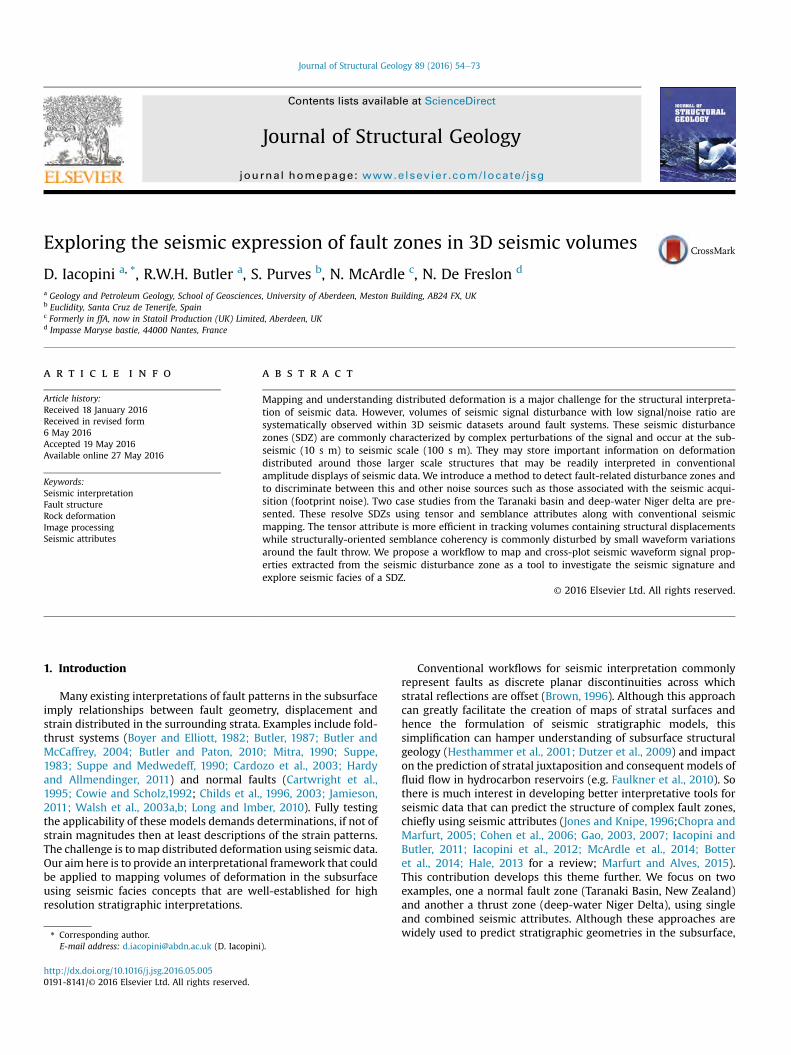
Some of the issues affecting structural interpretation of faultsare exemplified in Fig. 1. While some parts of the data appear toshowdiscrete offsets across narrow zones where seismic amplitudeis greatly reduced, other levels show broader areas of amplitudereduction. This could represent zones of more broadly disperseddeformation, such as are found in fault relays (Childs et al., 1996,2003; Walsh et al., 1991, 2002, 2003a,b). An indication of thesebroader deformation zones is manifest here as the folding of stratalreflectors both in the hangingwall and footwall to the fault zone.

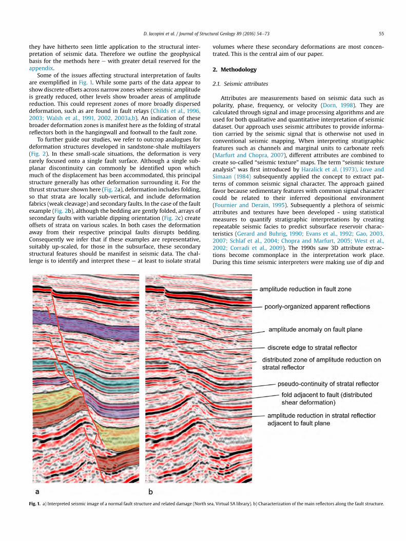
To further guide our studies, we refer to outcrop analogues fordeformation structures developed in sandstone-shale multilayers(Fig. 2). In these small-scale situations, the deformation is veryrarely focused onto a single fault surface. Although a single sub-planar discontinuity can commonly be identified upon whichmuch of the displacement has been accommodated, this principalstructure generally has other deformation surrounding it. For thethrust structure shown here (Fig. 2a), deformation includes folding,so that strata are locally sub-vertical, and include deformationfabrics (weak cleavage) and secondary faults. In the case of the faultexample (Fig. 2b), although the bedding are gently folded, arrays ofsecondary faults with variable dipping orientation (Fig. 2c) createoffsets of strata on various scales. In both cases the deformationaway from their respective principal faults disrupts bedding.Consequently we infer that if these examples are representative,suitably up-scaled, for those in the subsurface, these secondarystructural features should be manifest in seismic data. The chal-lenge is to identify and interpret these e at least to isolate stratal

Fig. 1. a) Interpreted seismic image of a normal fault structure and related damage (North se

volumes where these secondary deformations are most concen-trated. This is the central aim of our paper.

2. Methodology

2.1. Seismic attributes

Attributes are measurements based on seismic data such aspolarity, phase, frequency, or velocity (Dorn, 1998). They arecalculated through signal and image processing algorithms and areused for both qualitative and quantitative interpretation of seismicdataset. Our approach uses seismic attributes to provide informa-tion carried by the seismic signal that is otherwise not used inconventional seismic mapping. When interpreting stratigraphicfeatures such as channels and marginal units to carbonate reefs(Marfurt and Chopra, 2007), different attributes are combined tocreate so-called “seismic texture” maps. The term “seismic textureanalysis” was first introduced by Haralick et al. (1973). Love andSimaan (1984) subsequently applied the concept to extract pat-terns of common seismic signal character. The approach gainedfavor because sedimentary features with common signal charactercould be related to their inferred depositional environment(Fournier and Derain, 1995). Subsequently a plethora of seismicattributes and textures have been developed - using statisticalmeasures to quantify stratigraphic interpretations by creatingrepeatable seismic facies to predict subsurface reservoir charac-teristics (Gerard and Buhrig, 1990; Evans et al., 1992; Gao, 2003,2007; Schlaf et al., 2004; Chopra and Marfurt, 2005; West et al.,2002; Corradi et al., 2009). The 1990s saw 3D attribute extrac-tions become commonplace in the interpretation work place.During this time seismic interpreters were making use of dip and

a, Virtual SA library). b) Characterization of the main reflectors along the fault structure.

Fig. 2. a) View of a classical thrust structure, Prembokshire (UK). Arrows pointing respectively at thethrust fault and related anticline. b) thrust fault on turbidite complex, Army bay,New Zealand; c) zoomed view of b (black rectangle), on the small scale damage and fracture.

D. Iacopini et al. / Journal of Structural Geology 89 (2016) 54e7356

azimuth maps (Brown, 1996). Amplitude extractions and seismicsequence attribute mapping were also established (Chopra andMarfurt, 2007). In order to reveal subtle stratigraphic features(e.g. buried deltas, river channels, reefs and dewatering structures),datasets were pre conditioned (e.g. filtering random noise and precalculation of large scale linear or anisotropy features) leading tocross-correlation and coherence analysis (Marfurt and Chopra,2007). Further, dataset processing that preserved seismic ampli-tude has subsequently been used to infer porosity, statal thick-nesses and lithology. Computations of curvature on amplitude,envelope or impedance have proven efficient in describing struc-tural or channel lineament (Chopra and Marfurt, 2007, 2010). Herewe describe an equivalent single and multi-attributes analysis onpre-conditioned seismic datasets in order to characterize styles ofseismic response around selected larger scale deformation struc-tures that can otherwise be mapped conventionally using standardamplitude displays.

2.2. Noise analysis

Subsurface discontinuities create reflections and diffractions inseismic reflection data (Khaidukov et al., 2004). Reflections areused conventionally to interpret structural and stratigraphic fea-tures as they are generated by interfaces with impedance contrasts.Diffractions are generated by local discontinuities that act likepoint-sources (Neidell and Taner, 1971; Zavalishin, 2000),becoming active as soon as the direct wave hits them. Commonly, ifthose points are of the size comparable to the seismic wavelength(the Rayleigh criterion), they are ignored during processing

(Khaidukov et al., 2004). Consequently this imposes a limit on theresolution of recorded backscattered waves: below the Rayleighlimit (Moser and Howard, 2008; Gelius and Asgedom, 2011) nodefinite answers can be given as to location, dip, and curvature of adiscontinuity, nor its topological properties, such as connectivity.An example of these limits is illustrated in Fig. 3a, part of a dip lineextracted from a stacked 3D seismic volume. Here a discontinuity,inferred to represent a thrust fault, is surrounded by a halo char-acterized by low amplitude and incoherent seismic traces (thesquare box b Fig. 3a, b). The same characteristics are retained evenafter smoothing (Fig. 3c). This part of the seismic volume representsa width of several 10e100 m (see Fig. 3c for scale), which issignificantly larger than the Rayleigh limit of resolution. Thereforethis volume should contain primary reflections. That these areobscure suggests that the volume contains disruptive geologicalstructures e potentially deformation equivalent to that associatedwith outcropping faults (e.g. Fig. 2b). Dutzer et al. (2009) calledthese “seismic fault distortion zones”: volumes within the seismicdata of significant uncertainty where the signal is distorted.Iacopini and Butler (2011) termed these volumes of disruptedseismic signal “disturbance geobodies”, where geobodies areinterpreted 3-D objects that contain voxels with similar seismicamplitudes or other seismic attributes. Some disturbance geo-bodies, or components thereof, may relate to imaging problems(sensu Fagin, 1996), such as migration issues or/and interference bydiffractions due to the geometrical complication of strata and edgesaround the faults and folds. Others however may indeed representdeformation. Here we focus on the seismic properties and internalgeometry of disturbance geobodies by analysing the performance

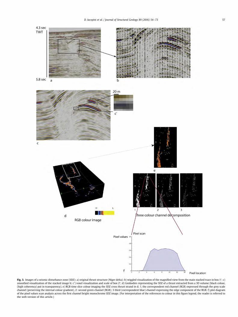
Fig. 3. Images of a seismic disturbance zone (SDZ): a) original thrust structure (Niger delta); b) wiggled visualization of the magnified view from the main stacked trace in box 10; c)smoothed visualization of the stacked image b; c0) voxel visualization and scale of box 20; d) Geobodies representing the SDZ of a thrust extracted from a 3D volume (black colour,(high coherency) put in transparency). e) RGB time slice colour imaging the SDZ cross thrust strand in d; 1. the correspondent red channel (RGB) expressed through the grey scalechannel (preserving the internal colour gradient), 2: second green channel (RGB); 3 third (correspondent blue) channel expressing the edge component of the RGB; f) plot diagramof the pixel values scan analysis across the first channel bright monochrome SDZ image. (For interpretation of the references to colour in this figure legend, the reader is referred tothe web version of this article.)

D. Iacopini et al. / Journal of Structural Geology 89 (2016) 54e73 57

D. Iacopini et al. / Journal of Structural Geology 89 (2016) 54e7358

of filters and filter sequences that can be applied during an image-processing workflow, especially those that inform interpretation ofthe distribution of the seismic noise within post stack seismicdatasets. We then introduce some simple cross-plotting techniquesso as to investigate the correlation between main phase andcoherence attributes and to define possible seismic facies withingeobodies. We believe that this approach can extend the use ofseismic data in extracting more geological information (at scalesabove the Rayleigh limit) to interpret signal distortions associatedwith larger-scale deformation structures.

2.3. Image processing techniques

Digital images, representing the seismic waveform, can besampled and converted to discrete valued integer numbers througha process of image quantization (Acharya and Ray, 2005). Thesmallest single sampled component of a digital image is a voxel.Any image is therefore subdivided into voxels (Fig. 3c0) and voxelcoordinates are indexed as amatrix of rows and columns. In seismicimage processing each voxel is associated with an intensity of thecolour that is proportional to the value of a particular attribute(Acharya and Ray, 2005 and Fig. 3f). The number of bits used torepresent the value of each voxel determines how many colours orshades of grey can be displayed and as a consequence how muchdetail we can expect to track in the signal analysis (Henderson et al.,2007, 2008). As an example see an image excerpt representing ageobody (Fig. 3d) that has been sliced (Fig. 3e) and decomposedacross three channels (1,2 and 3 in Fig. 3e) and then scannedthrough. The single colour brightness is associated with voxelvalues and can be easily extracted for further quantitative analysis.

Using processed images we can describe structurally-orienteddisturbed and low signal-to-noise zones surrounding faults andother deformed zones. Post-stack seismic data are used here. Weaim to demonstrate that such disturbed zones can be analyzedusing different coherency algorithms and cross-plotted through 3Dimage visualization and image processing tools. The image tech-niques and workflow proposed here can readily be represented andreproduced through a variety of image processing codes andcommercial/open source software (see also appendix).

3. The fault seismic disturbance zones (SDZ)

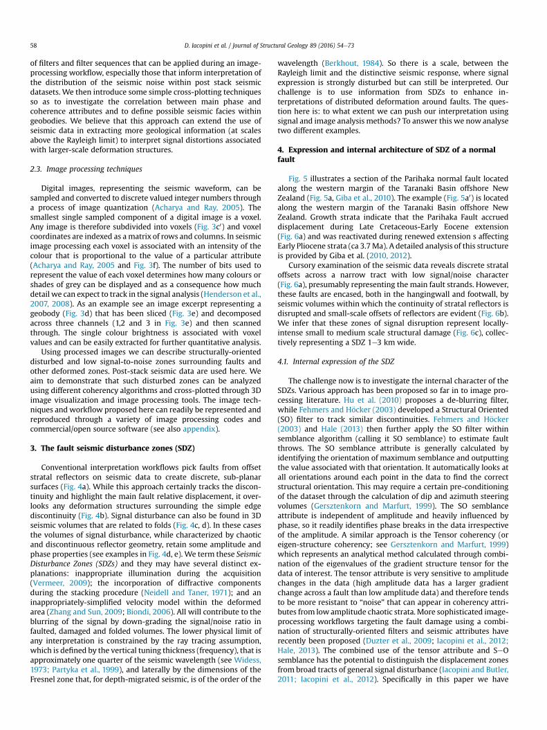
Conventional interpretation workflows pick faults from offsetstratal reflectors on seismic data to create discrete, sub-planarsurfaces (Fig. 4a). While this approach certainly tracks the discon-tinuity and highlight the main fault relative displacement, it over-looks any deformation structures surrounding the simple edgediscontinuity (Fig. 4b). Signal disturbance can also be found in 3Dseismic volumes that are related to folds (Fig. 4c, d). In these casesthe volumes of signal disturbance, while characterized by chaoticand discontinuous reflector geometry, retain some amplitude andphase properties (see examples in Fig. 4d, e). We term these SeismicDisturbance Zones (SDZs) and they may have several distinct ex-planations: inappropriate illumination during the acquisition(Vermeer, 2009); the incorporation of diffractive componentsduring the stacking procedure (Neidell and Taner, 1971); and aninappropriately-simplified velocity model within the deformedarea (Zhang and Sun, 2009; Biondi, 2006). All will contribute to theblurring of the signal by down-grading the signal/noise ratio infaulted, damaged and folded volumes. The lower physical limit ofany interpretation is constrained by the ray tracing assumption,which is defined by the vertical tuning thickness (frequency), that isapproximately one quarter of the seismic wavelength (see Widess,1973; Partyka et al., 1999), and laterally by the dimensions of theFresnel zone that, for depth-migrated seismic, is of the order of the

wavelength (Berkhout, 1984). So there is a scale, between theRayleigh limit and the distinctive seismic response, where signalexpression is strongly disturbed but can still be interpreted. Ourchallenge is to use information from SDZs to enhance in-terpretations of distributed deformation around faults. The ques-tion here is: to what extent we can push our interpretation usingsignal and image analysis methods? To answer this we now analysetwo different examples.

4. Expression and internal architecture of SDZ of a normalfault

Fig. 5 illustrates a section of the Parihaka normal fault locatedalong the western margin of the Taranaki Basin offshore NewZealand (Fig. 5a, Giba et al., 2010). The example (Fig. 5a0) is locatedalong the western margin of the Taranaki Basin offshore NewZealand. Growth strata indicate that the Parihaka Fault accrueddisplacement during Late Cretaceous-Early Eocene extension(Fig. 6a) and was reactivated during renewed extension s affectingEarly Pliocene strata (ca 3.7Ma). A detailed analysis of this structureis provided by Giba et al. (2010, 2012).

Cursory examination of the seismic data reveals discrete strataloffsets across a narrow tract with low signal/noise character(Fig. 6a), presumably representing the main fault strands. However,these faults are encased, both in the hangingwall and footwall, byseismic volumes within which the continuity of stratal reflectors isdisrupted and small-scale offsets of reflectors are evident (Fig. 6b).We infer that these zones of signal disruption represent locally-intense small to medium scale structural damage (Fig. 6c), collec-tively representing a SDZ 1e3 km wide.

4.1. Internal expression of the SDZ

The challenge now is to investigate the internal character of theSDZs. Various approach has been proposed so far in to image pro-cessing literature. Hu et al. (2010) proposes a de-blurring filter,while Fehmers and H€ocker (2003) developed a Structural Oriented(SO) filter to track similar discontinuities. Fehmers and H€ocker(2003) and Hale (2013) then further apply the SO filter withinsemblance algorithm (calling it SO semblance) to estimate faultthrows. The SO semblance attribute is generally calculated byidentifying the orientation of maximum semblance and outputtingthe value associated with that orientation. It automatically looks atall orientations around each point in the data to find the correctstructural orientation. This may require a certain pre-conditioningof the dataset through the calculation of dip and azimuth steeringvolumes (Gersztenkorn and Marfurt, 1999). The SO semblanceattribute is independent of amplitude and heavily influenced byphase, so it readily identifies phase breaks in the data irrespectiveof the amplitude. A similar approach is the Tensor coherency (oreigen-structure coherency; see Gersztenkorn and Marfurt, 1999)which represents an analytical method calculated through combi-nation of the eigenvalues of the gradient structure tensor for thedata of interest. The tensor attribute is very sensitive to amplitudechanges in the data (high amplitude data has a larger gradientchange across a fault than low amplitude data) and therefore tendsto be more resistant to “noise” that can appear in coherency attri-butes from lowamplitude chaotic strata. More sophisticated image-processing workflows targeting the fault damage using a combi-nation of structurally-oriented filters and seismic attributes haverecently been proposed (Duzter et al., 2009; Iacopini et al., 2012;Hale, 2013). The combined use of the tensor attribute and SeOsemblance has the potential to distinguish the displacement zonesfrom broad tracts of general signal disturbance (Iacopini and Butler,2011; Iacopini et al., 2012). Specifically in this paper we have

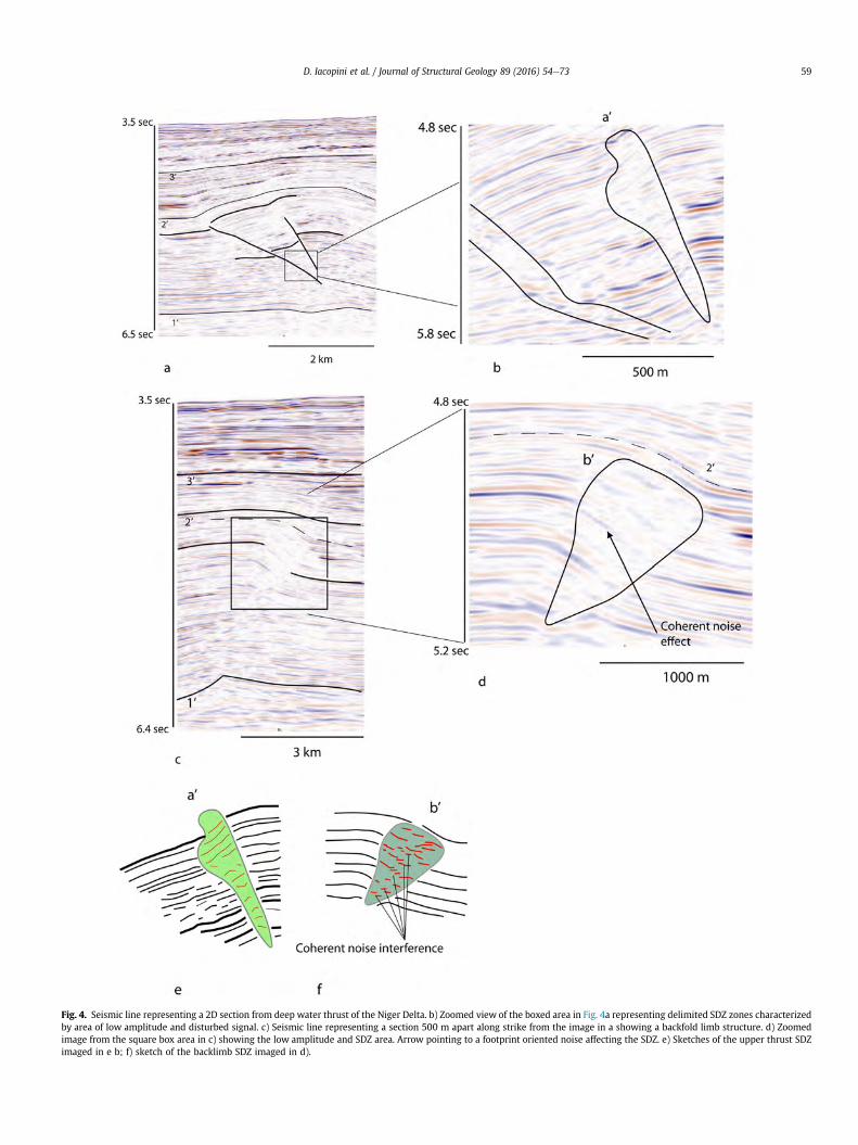
Fig. 4. Seismic line representing a 2D section from deep water thrust of the Niger Delta. b) Zoomed view of the boxed area in Fig. 4a representing delimited SDZ zones characterizedby area of low amplitude and disturbed signal. c) Seismic line representing a section 500 m apart along strike from the image in a showing a backfold limb structure. d) Zoomedimage from the square box area in c) showing the low amplitude and SDZ area. Arrow pointing to a footprint oriented noise affecting the SDZ. e) Sketches of the upper thrust SDZimaged in e b; f) sketch of the backlimb SDZ imaged in d).

D. Iacopini et al. / Journal of Structural Geology 89 (2016) 54e73 59

Fig. 5. a) Regional location of the Parihaka fault (modified from the New Zealand Ministry of Petroleum and Minerals regional map). b) Time slice semblance coherency visual-ization (at 900 ms TWT, within the upper Pleistocene) of the Parihaka fault. Section lines show the location of the seismic sections in Figs. 6 and 7. Rectangle shows time slices inFigs. 7d, e and 10. c) 3D visualization of the deepwater Niger delta thrust structure. The grey section traces represents the seismic image proposed in Figs. 4a, c and 9a, d. d) Locationof the deep water thrust system discussed and represented in Fig. 4c.

D. Iacopini et al. / Journal of Structural Geology 89 (2016) 54e7360

adopted a modified version of the main workflow proceduredescribed in Iacopini et al. (2012) and briefly highlighted in theAppendix. Taner et al. (1979) and Purves (2014) describe and

discuss the underlying physics associated with complex attributessuch as instantaneous phase.

In order to express the seismic texture of the main internal

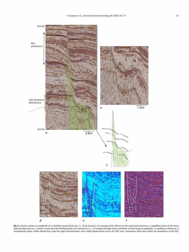
Fig. 6. Seismic sections in amplitude of: a) Parihaka normal fault (see Fig. 5b for location); b) zooming of the SDZ across the main fault structures; c) simplified sketch of the lowermain damage zones in c. Seismic section from the Parihaka fault (d to f, location in Fig. 5b) imaged through various attributes d) fault image in amplitude; e) semblance coherency; f)instantaneous phase. White dotted lines map the major discontinuities with visible displacement across the SDZ zone. Continuous white lines define the boundaries of the SDZ.

D. Iacopini et al. / Journal of Structural Geology 89 (2016) 54e73 61

D. Iacopini et al. / Journal of Structural Geology 89 (2016) 54e7362

structure of the SDZ, in our interpretation we analyse and comparethe amplitude, SO semblance coherency and the instantaneousphase expression of the signal. First we apply these three attributesto a segment of the fault (Fig. 5) and discuss their capabilities inenhancing different seismic aspects of the SDZ.

4.1.1. Amplitude expressionThe fault zone in Fig. 6d is surrounded by a SDZ of small-scale

faults that affect the continuity and coherency of the amplitudesignal. The SDZ includes not only the fault core zone (where thedisplacement is localized, as indicated by the white dotted lines)but also variable portions of the boundary walls where the signal isstrongly disturbed. This distributed zone varies in width between50 and 200 m.

4.1.2. SO semblance coherencyA semblance coherency image is represented in Fig. 6e. The

colour scale is set such that bright yellows represent low semblancevalues (strong variability of waveform properties across the traces)while blue colours represent high semblance coherency areas.Incoherency is found not only associated with the main disconti-nuities but also within the adjacent SDZ (bold white line) where itshows similar scattered low values of coherency. Using opacitycontrols, semblance can also track the main discontinuities in thestratal reflectors together with amplitude variations along thesereflectors.

4.1.3. Instantaneous phaseInstantaneous phase (the phase component of the Hilbert

transformation of the seismic dataset; Taner et al., 1979, Purves,2014) is effective at highlighting phase-dependent propertiessuch as thin bed-sets, reflection terminations and other disconti-nuities in stratal reflectors. This attribute is commonly used toenhance interpretations of discontinuous stratal patterns such asonlap and offlap (Chopra and Marfurt, 2007). Within the SDZ(Fig. 6f), reflectors are characterized by discontinuities and/orchaotic structures. The instantaneous phase attribute reveals sub-structure within SDZs that, using semblance, are not otherwiseimaged.

In the specific case studied here, the comparison of the imagesusing three different expressions (amplitude, semblance andinstantaneous phase) indicates that small scale faults are trackedand registered by coherency attributes and stratigraphicallyunraveled by phase-related attributes. It is through the combineduse of these various attributes that structural interpretation of thefaults is enhanced.

4.2. Image analysis of the tensor and SO semblance

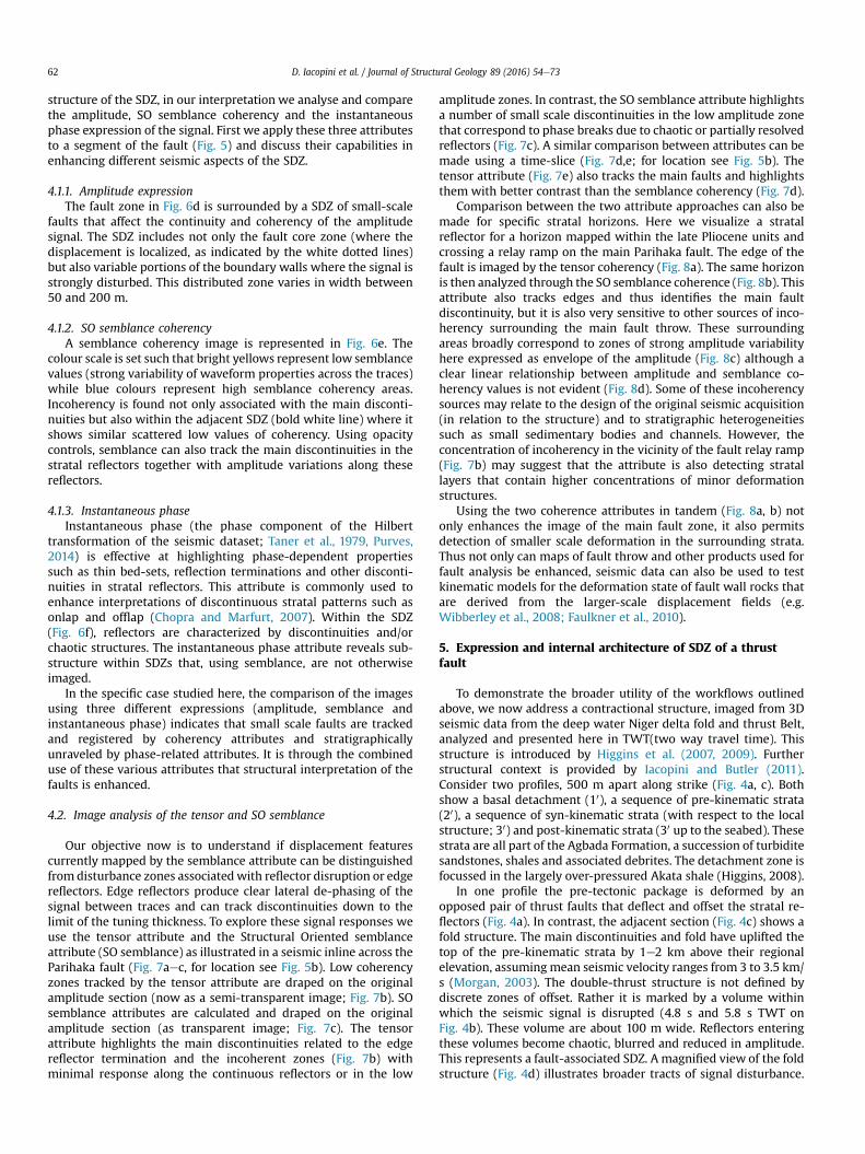
Our objective now is to understand if displacement featurescurrently mapped by the semblance attribute can be distinguishedfrom disturbance zones associatedwith reflector disruption or edgereflectors. Edge reflectors produce clear lateral de-phasing of thesignal between traces and can track discontinuities down to thelimit of the tuning thickness. To explore these signal responses weuse the tensor attribute and the Structural Oriented semblanceattribute (SO semblance) as illustrated in a seismic inline across theParihaka fault (Fig. 7aec, for location see Fig. 5b). Low coherencyzones tracked by the tensor attribute are draped on the originalamplitude section (now as a semi-transparent image; Fig. 7b). SOsemblance attributes are calculated and draped on the originalamplitude section (as transparent image; Fig. 7c). The tensorattribute highlights the main discontinuities related to the edgereflector termination and the incoherent zones (Fig. 7b) withminimal response along the continuous reflectors or in the low

amplitude zones. In contrast, the SO semblance attribute highlightsa number of small scale discontinuities in the low amplitude zonethat correspond to phase breaks due to chaotic or partially resolvedreflectors (Fig. 7c). A similar comparison between attributes can bemade using a time-slice (Fig. 7d,e; for location see Fig. 5b). Thetensor attribute (Fig. 7e) also tracks the main faults and highlightsthem with better contrast than the semblance coherency (Fig. 7d).

Comparison between the two attribute approaches can also bemade for specific stratal horizons. Here we visualize a stratalreflector for a horizon mapped within the late Pliocene units andcrossing a relay ramp on the main Parihaka fault. The edge of thefault is imaged by the tensor coherency (Fig. 8a). The same horizonis then analyzed through the SO semblance coherence (Fig. 8b). Thisattribute also tracks edges and thus identifies the main faultdiscontinuity, but it is also very sensitive to other sources of inco-herency surrounding the main fault throw. These surroundingareas broadly correspond to zones of strong amplitude variabilityhere expressed as envelope of the amplitude (Fig. 8c) although aclear linear relationship between amplitude and semblance co-herency values is not evident (Fig. 8d). Some of these incoherencysources may relate to the design of the original seismic acquisition(in relation to the structure) and to stratigraphic heterogeneitiessuch as small sedimentary bodies and channels. However, theconcentration of incoherency in the vicinity of the fault relay ramp(Fig. 7b) may suggest that the attribute is also detecting stratallayers that contain higher concentrations of minor deformationstructures.

Using the two coherence attributes in tandem (Fig. 8a, b) notonly enhances the image of the main fault zone, it also permitsdetection of smaller scale deformation in the surrounding strata.Thus not only can maps of fault throw and other products used forfault analysis be enhanced, seismic data can also be used to testkinematic models for the deformation state of fault wall rocks thatare derived from the larger-scale displacement fields (e.g.Wibberley et al., 2008; Faulkner et al., 2010).

5. Expression and internal architecture of SDZ of a thrustfault

To demonstrate the broader utility of the workflows outlinedabove, we now address a contractional structure, imaged from 3Dseismic data from the deep water Niger delta fold and thrust Belt,analyzed and presented here in TWT(two way travel time). Thisstructure is introduced by Higgins et al. (2007, 2009). Furtherstructural context is provided by Iacopini and Butler (2011).Consider two profiles, 500 m apart along strike (Fig. 4a, c). Bothshow a basal detachment (10), a sequence of pre-kinematic strata(20), a sequence of syn-kinematic strata (with respect to the localstructure; 30) and post-kinematic strata (30 up to the seabed). Thesestrata are all part of the Agbada Formation, a succession of turbiditesandstones, shales and associated debrites. The detachment zone isfocussed in the largely over-pressured Akata shale (Higgins, 2008).

In one profile the pre-tectonic package is deformed by anopposed pair of thrust faults that deflect and offset the stratal re-flectors (Fig. 4a). In contrast, the adjacent section (Fig. 4c) shows afold structure. The main discontinuities and fold have uplifted thetop of the pre-kinematic strata by 1e2 km above their regionalelevation, assumingmean seismic velocity ranges from 3 to 3.5 km/s (Morgan, 2003). The double-thrust structure is not defined bydiscrete zones of offset. Rather it is marked by a volume withinwhich the seismic signal is disrupted (4.8 s and 5.8 s TWT onFig. 4b). These volume are about 100 m wide. Reflectors enteringthese volumes become chaotic, blurred and reduced in amplitude.This represents a fault-associated SDZ. A magnified view of the foldstructure (Fig. 4d) illustrates broader tracts of signal disturbance.

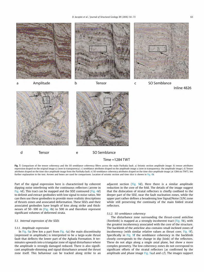
Fig. 7. Comparison of the tensor coherency and the SO semblance coherency filters across the main Parihaka fault. a) Seismic section amplitude image; b) tensor attributesexpression draped on the original image a) (now in transparency); c) semblance attributes draped on the amplitude image a (now in transparency: the amplitude image). d) Tensorattributes draped on the time slice amplitude image from the Parihaka fault; e) SO semblance coherency attributes draped on the time slice amplitude image (at 1284 ms TWT). Seefurther explanation in the text. Arrows and boxes are used for comparisons. Location of seismic section and time slice is shown in Fig. 6b.

D. Iacopini et al. / Journal of Structural Geology 89 (2016) 54e73 63

Part of the signal expression here is characterized by coherentdipping noise interfering with the continuous reflectors (arrow inFig. 4d). This tract can be mapped and the SDZ contoured (Fig. 4d)to delimit and extract geobodies with low signal to noise ratios. Wecan then use these geobodies to provide more realistic descriptionsof thrusts zones and associated deformation. These SDZs and theirassociated geobodies have length of kms along strike and thick-nesses of 50e100 m (Fig. 4b) to 500 m and therefore representsignificant volumes of deformed strata.

5.1. Internal expression of the SDZs

5.1.1. Amplitude expressionIn Fig. 9a (few km a part from Fig. 4a) the main discontinuity

(expressed in amplitude) is interpreted to be a large-scale thrustfault that deflects the lower part of the Agbada Formation. It ter-minates upwards into a triangular zone of signal disturbancewherethe amplitude is strongly damaged reduced. There is also signifi-cant amplitude-dimming and signal disturbance around the thrustzone itself. This behaviour can be tracked along strike to an

adjacent section (Fig. 9d). Here there is a similar amplitudereduction in the core of the fold. The details of the image suggestthat the dislocation of stratal reflectors is chiefly confined to thedeeper part of the SDZ, near the fault nucleation zones, while theupper part rather defines a broadening low Signal/Noise (S/N) zonewhile still preserving the continuity of the main folded stratalreflectors.

5.1.2. SO semblance coherencyThe disturbance zone surrounding the thrust-cored anticline

(forelimb) is mapped as a strongly incoherent tract (Fig. 9b), withthe greatest incoherency associated with the core of the structure.The backlimb of the anticline also contains small inclined zones ofincoherency (with similar relative values as thrust core; Fig. 9f).Specifically in Fig. 9f the semblance coherency in the backlimbclosely corresponds to the change in dip (kink) of the reflectors.These do not align along a single axial plane, but show a morecomplex geometry. The low coherency zones do not correspond tosignificant offsets of the stratal reflectors (as confirmed by theamplitude and phase image Fig. 9a,d and c,f). The images support

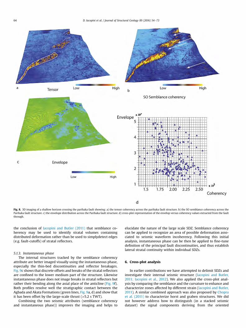
Fig. 8. 3D imaging of a shallow horizon crossing the parihaka fault showing: a) the tensor coherency across the parihaka fault structure. b) the SO semblance coherency across theParihaka fault structure. c) the envelope distribution across the Parihaka fault structure. d) cross-plot representation of the envelop versus coherency values extracted from the faultthrough.

D. Iacopini et al. / Journal of Structural Geology 89 (2016) 54e7364

the conclusion of Iacopini and Butler (2011) that semblance co-herency may be used to identify stratal volumes containingdistributed deformation rather than be used to simplydetect edges(e.g. fault-cutoffs) of stratal reflectors.

5.1.3. Instantaneous phaseThe internal structures tracked by the semblance coherency

attribute are better imaged visually using the instantaneous phase,especially the thin-bed discontinuities and reflector breakages.Fig. 9c shows that discrete offsets and breaks of the stratal reflectorsare confined to the lower medium part of the structure. Likewiseinstantaneous phase does not image breaks in stratal reflectors butrather their bending along the axial place of the anticline (Fig. 9f).Both profiles resolve well the stratigraphic contact between theAgbada and Akata Formations (green lines, Fig. 9a, d) and show thatit has been offset by the large-scale thrust (>5.2 s TWT).

Combining the two seismic attributes (semblance coherencyand instantaneous phase)) improves the imaging and helps to

elucidate the nature of the large scale SDZ. Semblance coherencycan be applied to recognize an area of possible deformation asso-ciated to seismic waveform incoherency. Following this initialanalysis, instantaneous phase can be then be applied to fine-tunedefinition of the principal fault discontinuities, and thus establishlateral stratal continuity within individual SDZs.

6. Cross-plot analysis

In earlier contributions we have attempted to delimit SDZs andinvestigate their internal seismic structure (Iacopini and Butler,2011; Iacopini et al., 2012). We also applied the cross-plot anal-ysis by comparing the semblance and the curvature to enhance andcharacterize zones affected by different strain (Iacopini and Butler,2011). A similar combined approach was also proposed by Chopraet al. (2011) to characterize horst and graben structures. We didnot however address how to distinguish (in a stacked seismicdataset) the signal components deriving from the oriented

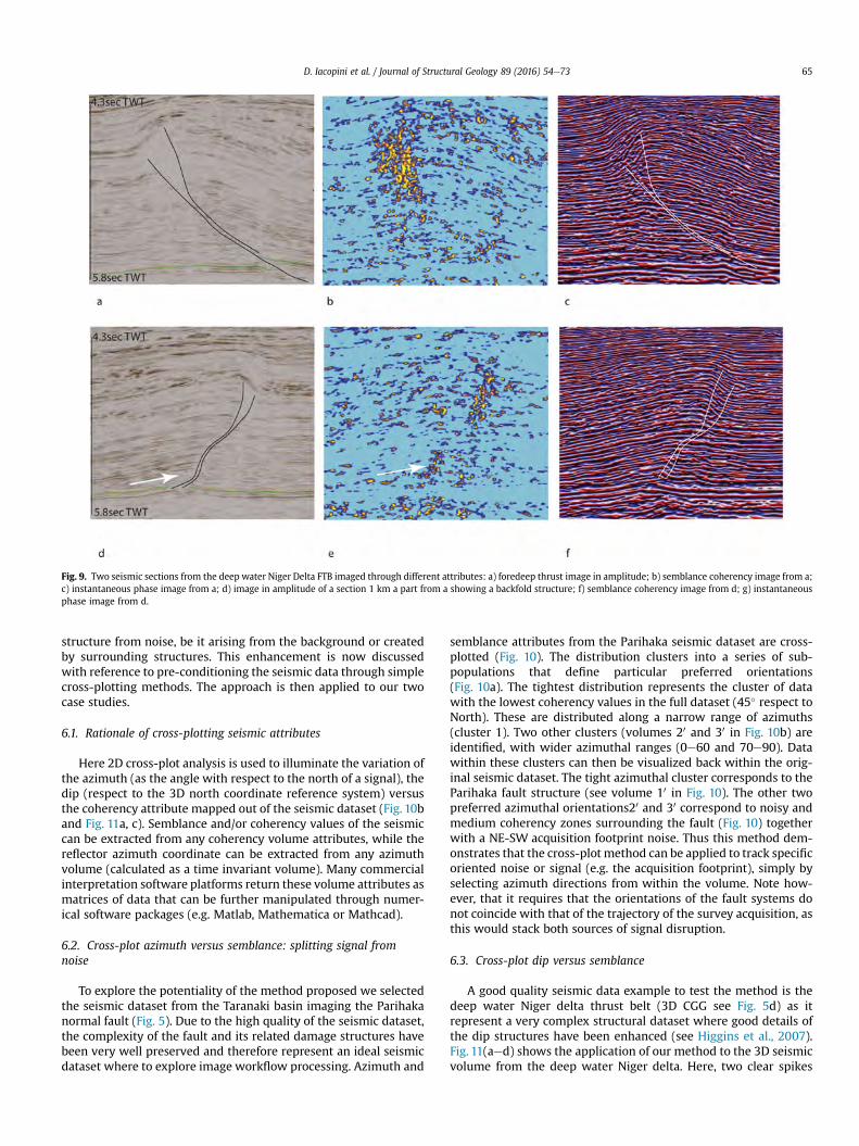
Fig. 9. Two seismic sections from the deep water Niger Delta FTB imaged through different attributes: a) foredeep thrust image in amplitude; b) semblance coherency image from a;c) instantaneous phase image from a; d) image in amplitude of a section 1 km a part from a showing a backfold structure; f) semblance coherency image from d; g) instantaneousphase image from d.

D. Iacopini et al. / Journal of Structural Geology 89 (2016) 54e73 65

structure from noise, be it arising from the background or createdby surrounding structures. This enhancement is now discussedwith reference to pre-conditioning the seismic data through simplecross-plotting methods. The approach is then applied to our twocase studies.

6.1. Rationale of cross-plotting seismic attributes

Here 2D cross-plot analysis is used to illuminate the variation ofthe azimuth (as the angle with respect to the north of a signal), thedip (respect to the 3D north coordinate reference system) versusthe coherency attribute mapped out of the seismic dataset (Fig. 10band Fig. 11a, c). Semblance and/or coherency values of the seismiccan be extracted from any coherency volume attributes, while thereflector azimuth coordinate can be extracted from any azimuthvolume (calculated as a time invariant volume). Many commercialinterpretation software platforms return these volume attributes asmatrices of data that can be further manipulated through numer-ical software packages (e.g. Matlab, Mathematica or Mathcad).

6.2. Cross-plot azimuth versus semblance: splitting signal fromnoise

To explore the potentiality of the method proposed we selectedthe seismic dataset from the Taranaki basin imaging the Parihakanormal fault (Fig. 5). Due to the high quality of the seismic dataset,the complexity of the fault and its related damage structures havebeen very well preserved and therefore represent an ideal seismicdataset where to explore image workflow processing. Azimuth and

semblance attributes from the Parihaka seismic dataset are cross-plotted (Fig. 10). The distribution clusters into a series of sub-populations that define particular preferred orientations(Fig. 10a). The tightest distribution represents the cluster of datawith the lowest coherency values in the full dataset (45� respect toNorth). These are distributed along a narrow range of azimuths(cluster 1). Two other clusters (volumes 20 and 30 in Fig. 10b) areidentified, with wider azimuthal ranges (0e60 and 70e90). Datawithin these clusters can then be visualized back within the orig-inal seismic dataset. The tight azimuthal cluster corresponds to theParihaka fault structure (see volume 10 in Fig. 10). The other twopreferred azimuthal orientations20 and 30 correspond to noisy andmedium coherency zones surrounding the fault (Fig. 10) togetherwith a NE-SW acquisition footprint noise. Thus this method dem-onstrates that the cross-plot method can be applied to track specificoriented noise or signal (e.g. the acquisition footprint), simply byselecting azimuth directions from within the volume. Note how-ever, that it requires that the orientations of the fault systems donot coincide with that of the trajectory of the survey acquisition, asthis would stack both sources of signal disruption.

6.3. Cross-plot dip versus semblance

A good quality seismic data example to test the method is thedeep water Niger delta thrust belt (3D CGG see Fig. 5d) as itrepresent a very complex structural dataset where good details ofthe dip structures have been enhanced (see Higgins et al., 2007).Fig. 11(aed) shows the application of our method to the 3D seismicvolume from the deep water Niger delta. Here, two clear spikes

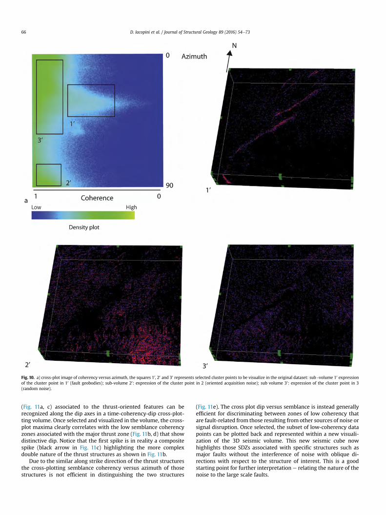
Fig. 10. a) cross-plot image of coherency versus azimuth, the squares 10, 20 and 30 represents selected cluster points to be visualize in the original dataset: sub -volume 10 expressionof the cluster point in 10 (fault geobodies); sub-volume 20: expression of the cluster point in 2 (oriented acquisition noise); sub volume 30: expression of the cluster point in 3(random noise).

D. Iacopini et al. / Journal of Structural Geology 89 (2016) 54e7366

(Fig. 11a, c) associated to the thrust-oriented features can berecognized along the dip axes in a time-coherency-dip cross-plot-ting volume. Once selected and visualized in the volume, the cross-plot maxima clearly correlates with the low semblance coherencyzones associated with the major thrust zone (Fig. 11b, d) that showdistinctive dip. Notice that the first spike is in reality a compositespike (black arrow in Fig. 11c) highlighting the more complexdouble nature of the thrust structures as shown in Fig. 11b.

Due to the similar along strike direction of the thrust structuresthe cross-plotting semblance coherency versus azimuth of thosestructures is not efficient in distinguishing the two structures

(Fig. 11e). The cross plot dip versus semblance is instead generallyefficient for discriminating between zones of low coherency thatare fault-related from those resulting from other sources of noise orsignal disruption. Once selected, the subset of low-coherency datapoints can be plotted back and represented within a new visuali-zation of the 3D seismic volume. This new seismic cube nowhighlights those SDZs associated with specific structures such asmajor faults without the interference of noise with oblique di-rections with respect to the structure of interest. This is a goodstarting point for further interpretation e relating the nature of thenoise to the large scale faults.

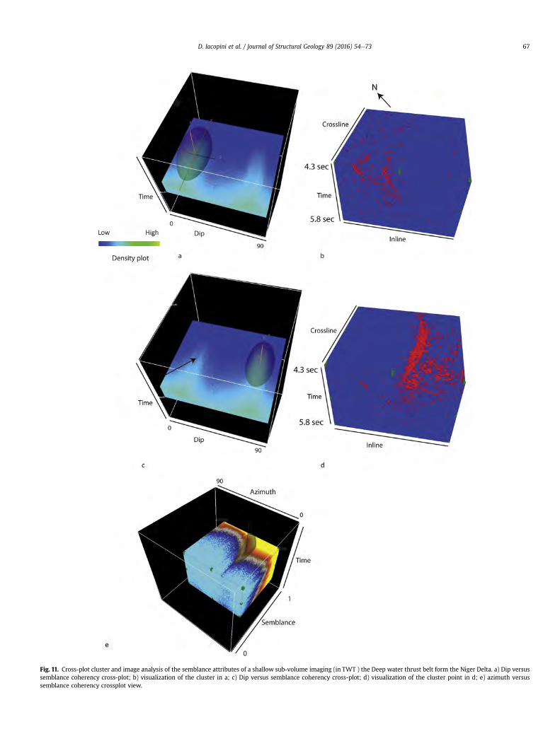
Fig. 11. Cross-plot cluster and image analysis of the semblance attributes of a shallow sub-volume imaging (in TWT ) the Deep water thrust belt form the Niger Delta. a) Dip versussemblance coherency cross-plot; b) visualization of the cluster in a; c) Dip versus semblance coherency cross-plot; d) visualization of the cluster point in d; e) azimuth versussemblance coherency crossplot view.

D. Iacopini et al. / Journal of Structural Geology 89 (2016) 54e73 67

D. Iacopini et al. / Journal of Structural Geology 89 (2016) 54e7368

7. Mapping and characterizing the disturbance zones

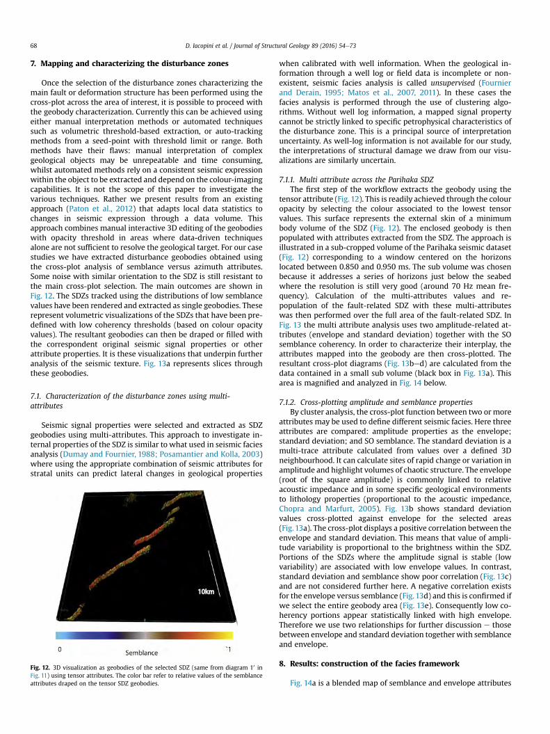
Once the selection of the disturbance zones characterizing themain fault or deformation structure has been performed using thecross-plot across the area of interest, it is possible to proceed withthe geobody characterization. Currently this can be achieved usingeither manual interpretation methods or automated techniquessuch as volumetric threshold-based extraction, or auto-trackingmethods from a seed-point with threshold limit or range. Bothmethods have their flaws: manual interpretation of complexgeological objects may be unrepeatable and time consuming,whilst automated methods rely on a consistent seismic expressionwithin the object to be extracted and depend on the colour-imagingcapabilities. It is not the scope of this paper to investigate thevarious techniques. Rather we present results from an existingapproach (Paton et al., 2012) that adapts local data statistics tochanges in seismic expression through a data volume. Thisapproach combines manual interactive 3D editing of the geobodieswith opacity threshold in areas where data-driven techniquesalone are not sufficient to resolve the geological target. For our casestudies we have extracted disturbance geobodies obtained usingthe cross-plot analysis of semblance versus azimuth attributes.Some noise with similar orientation to the SDZ is still resistant tothe main cross-plot selection. The main outcomes are shown inFig. 12. The SDZs tracked using the distributions of low semblancevalues have been rendered and extracted as single geobodies. Theserepresent volumetric visualizations of the SDZs that have been pre-defined with low coherency thresholds (based on colour opacityvalues). The resultant geobodies can then be draped or filled withthe correspondent original seismic signal properties or otherattribute properties. It is these visualizations that underpin furtheranalysis of the seismic texture. Fig. 13a represents slices throughthese geobodies.

7.1. Characterization of the disturbance zones using multi-attributes

Seismic signal properties were selected and extracted as SDZgeobodies using multi-attributes. This approach to investigate in-ternal properties of the SDZ is similar to what used in seismic faciesanalysis (Dumay and Fournier, 1988; Posamantier and Kolla, 2003)where using the appropriate combination of seismic attributes forstratal units can predict lateral changes in geological properties

Fig. 12. 3D visualization as geobodies of the selected SDZ (same from diagram 10 inFig. 11) using tensor attributes. The color bar refer to relative values of the semblanceattributes draped on the tensor SDZ geobodies.

when calibrated with well information. When the geological in-formation through a well log or field data is incomplete or non-existent, seismic facies analysis is called unsupervised (Fournierand Derain, 1995; Matos et al., 2007, 2011). In these cases thefacies analysis is performed through the use of clustering algo-rithms. Without well log information, a mapped signal propertycannot be strictly linked to specific petrophysical characteristics ofthe disturbance zone. This is a principal source of interpretationuncertainty. As well-log information is not available for our study,the interpretations of structural damage we draw from our visu-alizations are similarly uncertain.

7.1.1. Multi attribute across the Parihaka SDZThe first step of the workflow extracts the geobody using the

tensor attribute (Fig. 12). This is readily achieved through the colouropacity by selecting the colour associated to the lowest tensorvalues. This surface represents the external skin of a minimumbody volume of the SDZ (Fig. 12). The enclosed geobody is thenpopulated with attributes extracted from the SDZ. The approach isillustrated in a sub-cropped volume of the Parihaka seismic dataset(Fig. 12) corresponding to a window centered on the horizonslocated between 0.850 and 0.950 ms. The sub volume was chosenbecause it addresses a series of horizons just below the seabedwhere the resolution is still very good (around 70 Hz mean fre-quency). Calculation of the multi-attributes values and re-population of the fault-related SDZ with these multi-attributeswas then performed over the full area of the fault-related SDZ. InFig. 13 the multi attribute analysis uses two amplitude-related at-tributes (envelope and standard deviation) together with the SOsemblance coherency. In order to characterize their interplay, theattributes mapped into the geobody are then cross-plotted. Theresultant cross-plot diagrams (Fig. 13bed) are calculated from thedata contained in a small sub volume (black box in Fig. 13a). Thisarea is magnified and analyzed in Fig. 14 below.

7.1.2. Cross-plotting amplitude and semblance propertiesBy cluster analysis, the cross-plot function between two or more

attributes may be used to define different seismic facies. Here threeattributes are compared: amplitude properties as the envelope;standard deviation; and SO semblance. The standard deviation is amulti-trace attribute calculated from values over a defined 3Dneighbourhood. It can calculate sites of rapid change or variation inamplitude and highlight volumes of chaotic structure. The envelope(root of the square amplitude) is commonly linked to relativeacoustic impedance and in some specific geological environmentsto lithology properties (proportional to the acoustic impedance,Chopra and Marfurt, 2005). Fig. 13b shows standard deviationvalues cross-plotted against envelope for the selected areas(Fig.13a). The cross-plot displays a positive correlation between theenvelope and standard deviation. This means that value of ampli-tude variability is proportional to the brightness within the SDZ.Portions of the SDZs where the amplitude signal is stable (lowvariability) are associated with low envelope values. In contrast,standard deviation and semblance show poor correlation (Fig. 13c)and are not considered further here. A negative correlation existsfor the envelope versus semblance (Fig.13d) and this is confirmed ifwe select the entire geobody area (Fig. 13e). Consequently low co-herency portions appear statistically linked with high envelope.Therefore we use two relationships for further discussion e thosebetween envelope and standard deviation together with semblanceand envelope.

8. Results: construction of the facies framework

Fig. 14a is a blended map of semblance and envelope attributes

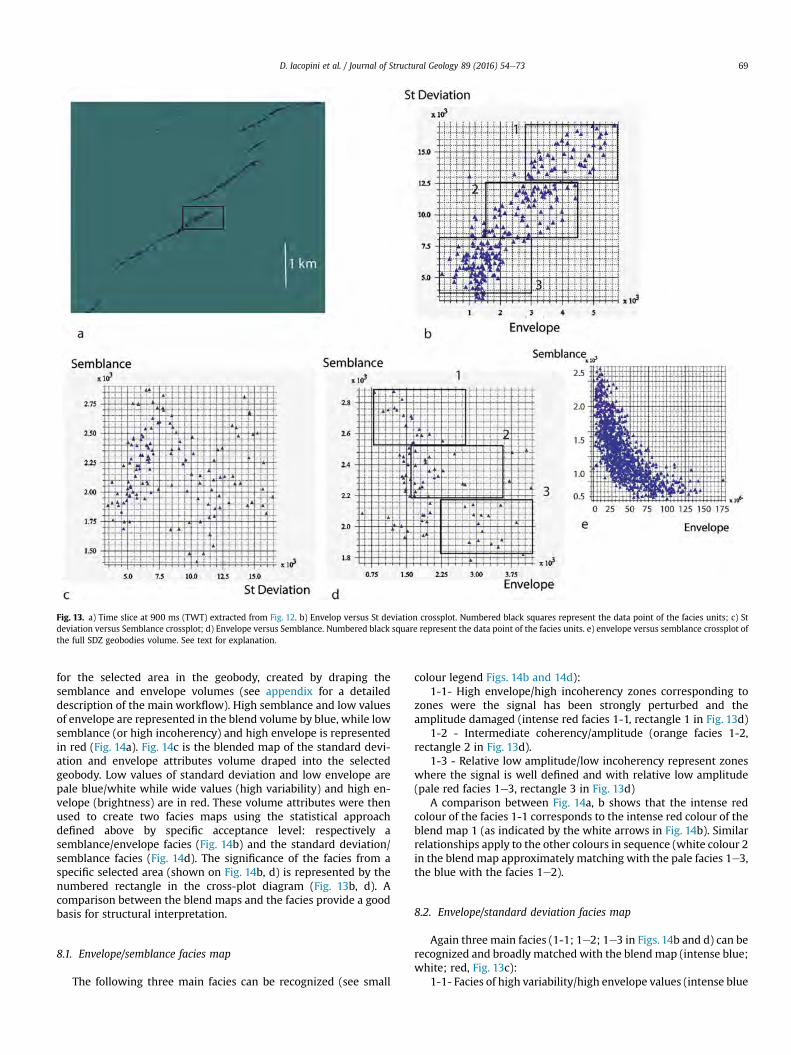
Fig. 13. a) Time slice at 900 ms (TWT) extracted from Fig. 12. b) Envelop versus St deviation crossplot. Numbered black squares represent the data point of the facies units; c) Stdeviation versus Semblance crossplot; d) Envelope versus Semblance. Numbered black square represent the data point of the facies units. e) envelope versus semblance crossplot ofthe full SDZ geobodies volume. See text for explanation.

D. Iacopini et al. / Journal of Structural Geology 89 (2016) 54e73 69

for the selected area in the geobody, created by draping thesemblance and envelope volumes (see appendix for a detaileddescription of the main workflow). High semblance and low valuesof envelope are represented in the blend volume by blue, while lowsemblance (or high incoherency) and high envelope is representedin red (Fig. 14a). Fig. 14c is the blended map of the standard devi-ation and envelope attributes volume draped into the selectedgeobody. Low values of standard deviation and low envelope arepale blue/white while wide values (high variability) and high en-velope (brightness) are in red. These volume attributes were thenused to create two facies maps using the statistical approachdefined above by specific acceptance level: respectively asemblance/envelope facies (Fig. 14b) and the standard deviation/semblance facies (Fig. 14d). The significance of the facies from aspecific selected area (shown on Fig. 14b, d) is represented by thenumbered rectangle in the cross-plot diagram (Fig. 13b, d). Acomparison between the blend maps and the facies provide a goodbasis for structural interpretation.

8.1. Envelope/semblance facies map

The following three main facies can be recognized (see small

colour legend Figs. 14b and 14d):1-1- High envelope/high incoherency zones corresponding to

zones were the signal has been strongly perturbed and theamplitude damaged (intense red facies 1-1, rectangle 1 in Fig. 13d)

1-2 - Intermediate coherency/amplitude (orange facies 1-2,rectangle 2 in Fig. 13d).

1-3 - Relative low amplitude/low incoherency represent zoneswhere the signal is well defined and with relative low amplitude(pale red facies 1e3, rectangle 3 in Fig. 13d)

A comparison between Fig. 14a, b shows that the intense redcolour of the facies 1-1 corresponds to the intense red colour of theblend map 1 (as indicated by the white arrows in Fig. 14b). Similarrelationships apply to the other colours in sequence (white colour 2in the blend map approximately matching with the pale facies 1e3,the blue with the facies 1e2).

8.2. Envelope/standard deviation facies map

Again three main facies (1-1; 1e2; 1e3 in Figs. 14b and d) can berecognized and broadly matched with the blendmap (intense blue;white; red, Fig. 13c):

1-1- Facies of high variability/high envelope values (intense blue

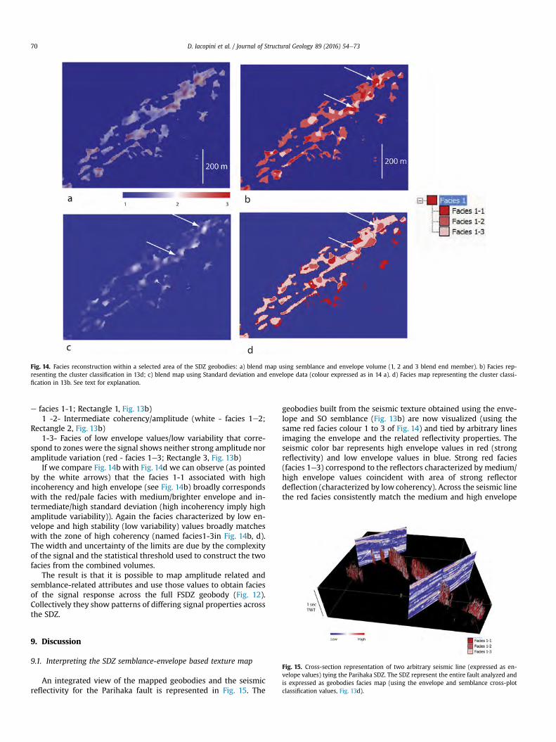
Fig. 14. Facies reconstruction within a selected area of the SDZ geobodies: a) blend map using semblance and envelope volume (1, 2 and 3 blend end member). b) Facies rep-resenting the cluster classification in 13d; c) blend map using Standard deviation and envelope data (colour expressed as in 14 a). d) Facies map representing the cluster classi-fication in 13b. See text for explanation.

D. Iacopini et al. / Journal of Structural Geology 89 (2016) 54e7370

e facies 1-1; Rectangle 1, Fig. 13b)1 -2- Intermediate coherency/amplitude (white - facies 1e2;

Rectangle 2, Fig. 13b)1-3- Facies of low envelope values/low variability that corre-

spond to zones were the signal shows neither strong amplitude noramplitude variation (red - facies 1e3; Rectangle 3, Fig. 13b)

If we compare Fig. 14b with Fig. 14d we can observe (as pointedby the white arrows) that the facies 1-1 associated with highincoherency and high envelope (see Fig. 14b) broadly correspondswith the red/pale facies with medium/brighter envelope and in-termediate/high standard deviation (high incoherency imply highamplitude variability)). Again the facies characterized by low en-velope and high stability (low variability) values broadly matcheswith the zone of high coherency (named facies1-3in Fig. 14b, d).The width and uncertainty of the limits are due by the complexityof the signal and the statistical threshold used to construct the twofacies from the combined volumes.

The result is that it is possible to map amplitude related andsemblance-related attributes and use those values to obtain faciesof the signal response across the full FSDZ geobody (Fig. 12).Collectively they show patterns of differing signal properties acrossthe SDZ.

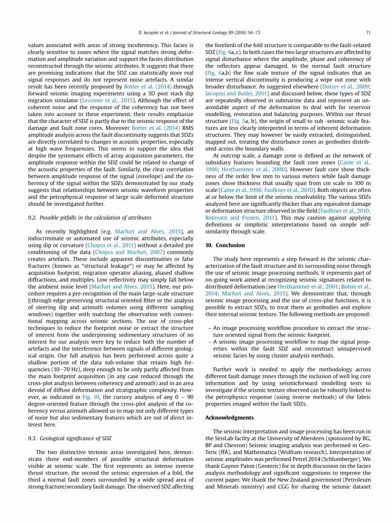
Fig. 15. Cross-section representation of two arbitrary seismic line (expressed as en-velope values) tying the Parihaka SDZ. The SDZ represent the entire fault analyzed andis expressed as geobodies facies map (using the envelope and semblance cross-plotclassification values, Fig. 13d).

9. Discussion

9.1. Interpreting the SDZ semblance-envelope based texture map

An integrated view of the mapped geobodies and the seismicreflectivity for the Parihaka fault is represented in Fig. 15. The

geobodies built from the seismic texture obtained using the enve-lope and SO semblance (Fig. 13b) are now visualized (using thesame red facies colour 1 to 3 of Fig. 14) and tied by arbitrary linesimaging the envelope and the related reflectivity properties. Theseismic color bar represents high envelope values in red (strongreflectivity) and low envelope values in blue. Strong red facies(facies 1e3) correspond to the reflectors characterized by medium/high envelope values coincident with area of strong reflectordeflection (characterized by low coherency). Across the seismic linethe red facies consistently match the medium and high envelope

D. Iacopini et al. / Journal of Structural Geology 89 (2016) 54e73 71

values associated with areas of strong incoherency. This facies isclearly sensitive to zones where the signal matches strong defor-mation and amplitude variation and support the facies distributionreconstructed through the seismic attributes. It suggests that thereare promising indications that the SDZ can statistically store realsignal responses and do not represent noise artefacts. A similarresult has been recently proposed by Botter et al. (2014) throughforward seismic imaging experiments using a 3D post stack dipmigration simulator (Lecomte et al., 2015). Although the effect ofcoherent noise and the response of the coherency has not beentaken into account in these experiment, their results emphasizethat the character of SDZ is partly due to the seismic response of thedamage and fault zone cores. Moreover Botter et al. (2014) RMSamplitude analysis across the fault discontinuity suggests that SDZsare directly correlated to changes in acoustic properties, especiallyat high wave frequencies. This seems to support the idea thatdespite the systematic effects of array acquisition parameters, theamplitude response within the SDZ could be related to change ofthe acoustic properties of the fault. Similarly, the clear correlationbetween amplitude response of the signal (envelope) and the co-herency of the signal within the SDZs demonstrated by our studysuggests that relationships between seismic waveform propertiesand the petrophysical response of large scale deformed structureshould be investigated further.

9.2. Possible pitfalls in the calculation of attributes

As recently highlighted (e.g. Marfurt and Alves, 2015), anindiscriminate or automated use of seismic attributes, especiallyusing dip or curvature (Chopra et al., 2011) without a detailed preconditioning of the data (Chopra and Marfurt, 2007) commonlycreates artefacts. These include apparent discontinuities or falsefractures (known as “structural leakage”) or may be affected byacquisition footprint, migration operator aliasing, aliased shallowdiffractions, and multiples. Low reflectivity may simply fall belowthe ambient noise level (Marfurt and Alves, 2015). Here, our pro-cedure requires a pre-recognition of the main large-scale structure|(through edge preserving structural oriented filter or the analysisof steering dip and azimuth volumes using different samplingwindows) together with matching the observation with conven-tional mapping across seismic sections. The use of cross-plottechniques to reduce the footprint noise or extract the structureof interest from the underpinning sedimentary structures of nointerest for our analysis were key to reduce both the number ofartefacts and the interference between signals of different geolog-ical origin. Our full analysis has been performed across quite ashallow portion of the data sub-volume that retains high fre-quencies (10e70 Hz), deep enough to be only partly affected fromthe main footprint acquisition (in any case reduced through thecross-plot analysis between coherency and azimuth) and in an areadevoid of diffuse deformation and stratigraphic complexity. How-ever, as indicated in Fig. 10, the cursory analysis of any 0 e 90degree-oriented feature through the cross-plot analysis of the co-herency versus azimuth allowed us to map not only different typesof noise but also sedimentary features which are not of direct in-terest here.

9.3. Geological significance of SDZ

The two distinctive tectonic areas investigated here, demon-strate three end-members of possible structural deformationvisible at seismic scale. The first represents an intense inversethrust structure, the second the seismic expression of a fold, thethird a normal fault zones surrounded by a wide spread area ofstrong fracture/secondary fault damage. The observed SDZ affecting

the forelimb of the fold structure is comparable to the fault-relatedSDZ (Fig. 4a, c). In both cases the two large structures are affected bysignal disturbance where the amplitude, phase and coherency ofthe reflectors appear damaged. In the normal fault structure(Fig. 6a,b) the fine scale texture of the signal indicates that anintense vertical discontinuity is producing a wipe out zone withbroader disturbance. As suggested elsewhere (Dutzer et al., 2009;Iacopini and Butler, 2011) and discussed below, these types of SDZare repeatedly observed in submarine data and represent an un-avoidable aspect of the deformation to deal with for reservoirmodelling, restoration and balancing purposes. Within our thruststructure (Fig. 3a, b), the origin of small to sub -seismic scale fea-tures are less clearly interpreted in terms of inherent deformationstructures. They may however be easily extracted, distinguished,mapped out, treating the disturbance zones as geobodies distrib-uted across the boundary walls.

At outcrop scale, a damage zone is defined as the network ofsubsidiary features bounding the fault core zones (Caine et al.,1996; Hesthammer et al., 2000). However fault core show thick-ness of the order few mm to various meters while fault damagezones show thickness that usually span from cm scale to 100 mscale (Caine et al., 1996; Faulkner et al., 2010). Both objects are oftenat or below the limit of the seismic resolvability. The various SDZsanalyzed here are significantly thicker than any equivalent damageor deformation structure observed in the field (Faulkner et al., 2010;Rotevatn and Fossen, 2011). This may caution against applyingdefinitions or simplistic interpretations based on simple self-similarity through scale.

10. Conclusion

The study here represents a step forward in the seismic char-acterization of the fault structure and its surrounding noise throughthe use of seismic image processing methods. It represents part ofon-going work aimed at recognizing seismic signatures related todistributed deformation (see Hesthammer et al., 2001; Botter et al.,2014; Marfurt and Alves, 2015). We demonstrate that, throughseismic image processing and the use of cross-plot functions, it ispossible to extract SDZs, to treat them as geobodies and exploretheir internal seismic texture. The followingmethods are proposed:

- An image processing workflow procedure to extract the struc-ture oriented signal from the seismic footprint.

- A seismic image processing workflow to map the signal prop-erties within the fault SDZ and reconstruct unsupervisedseismic facies by using cluster analysis methods.

Further work is needed to apply the methodology acrossdifferent fault damage zones through the inclusion of well log coreinformation and by using seismicforward modelling tests toinvestigate if the seismic texture observed can be robustly linked tothe petrophysics response (using inverse methods) of the fabricproperties imaged within the fault SDZs.

Acknowledgments

The seismic interpretation and image processing has been run inthe SeisLab facilty at the University of Aberdeen (sponsored by BG,BP and Chevron) Seismic imaging analysis was performed in Geo-Teric (ffA), and Mathematica (Wolfram research). Interpretation ofseismic amplitudes was performed Petrel 2014 (Schlumberger). Wethank Gaynor Paton (Geoteric) for in depth discussion on the faciesanalysis methodology and significant suggestions to improve thecurrent paper. We thank the New Zealand government (Petroleumand Minerals ministry) and CGG for sharing the seismic dataset

D. Iacopini et al. / Journal of Structural Geology 89 (2016) 54e7372

utilized in this research paper. Seismic images used here areavailable through the Virtual Seismic Atlas (www.seismicatlas.org).Nestor Cardozo and an anonymous reviewer are thanked for theirconstructive comments and suggestions that strongly improved thequality and organization of this paper.

Appendix A. Supplementary data

Supplementary data related to this article can be found at http://dx.doi.org/10.1016/j.jsg.2016.05.005

References

Acharya, I., Ray, A.K., 2005. Image Processing: Principles and Applications. Wiley,p. 452.

Berkhout, A.J., 1984. Seismic Exploration-seismic Resolution: a Quantitative Anal-ysis of Resolving Power of Acoustical Echo Techniques. Geophysical Press,London.

Biondi, B., 2006. 3D seismic imaging. SEG. Investig. Geophys. 14.Botter, C., Cardozo, N., Hardy, S., Leconte, I., Escalona, 2014. From mechanical

modeling to seismic imaging of faults: a synthetic workflow to study the impactof faults on seismic. Mar. Pet. Geol. 57, 187e207.

Boyer, S.J., Elliott, D., 1982. Thrust systems. Bull. Am. Assoc. Pet. Geol. 66, 1196e1230.Brown, A., 1996. Interpretation of Three-dimensional Seismic Data, seventh ed.Butler, R.H.W., McCaffrey, W.D., 2004. Nature of the thrust zones in deep water

sand-shale sequences:outcrop examples from the Champsaur sandstones of SEFrance. Mar. Pet. Geol. 21, 911e921.

Butler, R.W.H., Paton, D.A., 2010. Evaluating lateral compaction in deepwater foldand thrust belts: how much are we missing from Nature’s Sandbox? GSA Today20, 4e10.

Butler, R.W.H., 1987. Thrust sequences. J. Geol. Soc. 144, 619e634.Caine, J.S., Evans, J.P., Forster, C.B., 1996. Fault zone architecture and permeability

structure. Geology 24, 1025e1028.Cardozo, N., Bhalla, K., Zehnder, A.T., Allmendinger, R.W., 2003. Mechanical models

of fault propagation folds and comparison to the trishear kinematic model.J. Struct. Geol. 25, 1e18.

Cartwright, J.A., Trudgill, B.D., Mansfield, C.S., 1995. Fault growth by segment link-age; an explanation for scatter in maximum displacement and trace length datafromthe Canyonlands Grabens of SE Utah. J. Struct. Geol. 17, 1319e1326.

Childs, C., Nicol, A., Walsh, J.J., Watterson, J., 1996. Growth of vertically segmentednormal faults. J. Struct. Geol. 18, 1389e1397.

Childs, C., Nicol, A., Walsh, J.J., Watterson, J., 2003. The growth and propagation ofsyn sedimentary faults. J. Struct. Geol. 25, 633e648.

Chopra, S., Marfurt, K.J., 2005. Seismic Attributes e a historical perspective.Geophysics 70, 3e28.

Chopra, S., Marfurt, K.J., 2007. Curvature attribute applications to 3D seismic data.Lead. Edge 26 (4), 404e414.

Chopra, Marfurt, K.J., 2010. Integration of coherence and volumetric curvaturesimages. Lead. Edge 30, 1092e1106.

Chopra, S., Misra, S., Marfurt, K., 2011. Coherence and curvature attributes on pre-conditioned seismic dataset. Lead. Edge 32, 260e266.

Cohen, I., Coult, N., Vassiliou, A., 2006. Detection and extraction of fault surfaces in3D seismic data. Geophysics 71, 21e27.

Corradi, a., Ruffo, P., Visentin, C., 2009. 3D hydrocarbon migration by percolationtechnique in an alternate sandeshale environment described by a seismic faciesclassified volume. Mar. Pet. Geol. 26, 495e503.

Cowie, P.A., Scholz, C.H., 1992. Displacement-length scaling relationship for faults;data synthesis and discussion. J. Struct. Geol. 14, 1149e1156.

Dorn, G.A., 1998. Modern 3-D seismic interpretation. The Leading Edge 17 (9).http://dx.doi.org/10.1190/1.143, 1262-1262.

Dumay, J., Fournier, F., 1988. Multivariate statistical analyses applied to seismicfacies recognition. Geophysics 53, 1151e1159.

Dutzer, J.F., Basford, H., Purves, S., 2009. Investigating fault sealing potential throughfault relative seismic volume analysis. Pet. Geol. Conf. Ser. 7, 509e515. http://dx.doi.org/10.1144/0070509.

Evans, D.J., Meneilly, A., Brown, G., 1992. Seismic facies analysis of Westphaliansequences of the southern North Sea. Mar. Pet. Geol. 9, 578e589.

Fagin, 1996. The fault shadow problem: its nature and elimination. Lead. Edge 15,1005e1013.

Faulkner, D.R., Jackson, C.A.L., Lunn, R., Schlisch, R., Shipton, Z., Wibberley, C.,Withjack, M., 2010. A review of recent developments regarding the structure,mechanics and fluid flow properties of fault zones. J. Struct. Geol. 32,1557e1575.

Fehmers, G., H€ocker, C., 2003. Fast structural interpretation with structure-orientedfiltering. Geophysics 68, 1286e1293. http://dx.doi.org/10.1190/1.1598121.

Fournier, F., Derain, J.F., 1995. A statistical methodology for deriving reservoirproperties from seismic data. Geophysics 60, 1437e1450.

Gao, D., 2003. Volume texture extraction for 3D seismic visualization and inter-pretation. Geophysics 68, 1294e1302.

Gao, D., 2007. Application of three-dimensional seismic texture analysis with spe-cial reference to deep-marine facies discrimination and interpretation: offshore

Angola, West Africa. AAPG Bull. 91, 1665e1683.Gelius, L.J., Asgedom, E., 2011. Diffraction e limited imaging and beyond-the

concept of super resolution. Geophys. Prospect. 59, 400e421.Gerard, J., Buhrig, C., 1990. Seismic facies of the Permian section of the Barents

Shelf: analysis and interpretation. Mar. Pet. Geol. 7, 234e252.Gersztenkorn, G., Marfurt, K.J., 1999. Eigenstructure-based coherence computations

as an aid to 3-D structural and stratigraphic mapping. Geophysics 64,1468e1479.

Giba, M., Nicol, A., Walsh, J.J., 2010. Evolution of faulting and volcanism in a Back-Arc Basin and its implications for subduction processes. Tectonic 29, TC4020.

Giba, M., Walsh, J.J., Nicol, A., 2012. Segmentation and growth of an obliquelyreactivated normal fault. J. Struct. Geol. 39, 253e267.

Hale, D., 2013. Methods to compute fault images, extract fault surfaces and estimatefault throws from 3D seismic images. Geophysics 78, 33e43.

Haralick, R.M., Shanmugam, K., Dinstein, I., 1973. Textural features for image clas-sification. IEEE Trans. Syst. Man Cybern. 3, 610e621.

Hardy, S., Allmendinger, R., 2011. Trishear. A review of kinematics, mechanics, and783 applications. In: McClay, K., Shaaw, J., Suppe, J. (Eds.), Thrust Fault-relatedFolding, vol. 94. American Association of Petroleum Geologists Memoir,pp. 95e119.

Henderson, J., Purves, S., Leppard, C., 2007. Automated delineation of geologicalelements from 3D seismic data through analysis of multi-channel, volumetricspectral decomposition data. First Break 25, 87e93.

Henderson, J., Purves, S., Fisher, G., Leppard, C., 2008. Delineation of geological el-ements from RGB color blending of seismic attribute volume. Lead. Edge 8,342e349.

Hesthammer, J., Johansen, T.E.S., Watts, L., 2000. Spatial relationships within faultdamage zones in sandstone. Mar. Pet. Geol. 17, 873e893.

Hesthammer, J., Landrø, M., Fossen, H., 2001. Use and abuse of seismic data inreservoir characterisation. Mar. Pet. Geol. 18, 635e655.

Higgins, S., Davies, R.J., Clarke, B., 2007. Antithetic fault linkages in a deep water foldand thrust belt. J. Struct. Geol. 29, 1900e1914.

Higgins, S., Clarke, B., Davies, R.J., Cartwright, J., 2009. Internal geometry and growthhistory of a thrust-related anticline in a deep water fold belt. J. Struct. Geol. 31,1597e1611.

Hu, Z., Huang, J.B., Yang, M.H., 2010. Single Image deblurring with adaptive dic-tionary learning. In: IEEE international conference on image processing. China,Hong Kong, pp. 1169e1172.

Iacopini, D., Butler, R.W.H., 2011. Imaging deformation in submarine thrust beltsusing seismic attributes. Earth Planet. Sci. Lett. 302, 414e422.

Iacopini, D., Butler, R.W.H., Purves, S., 2012. Seismic imaging of thrust faults andstructural damage: a visualization workflow for deepwater thrust belts. FirstBreak 30, 39e46.

Jamieson, W.J., 2011. Geometrical analysis of fold development in overthrustterrane. J. Struct. Geol. 9, 207e219.

Jones, G., Knipe, R.J., 1996. Seismic attribute maps; application to structural inter-pretation and fault seal analysis in the North Sea Basin. First Break 14, 10e12.

Khaidukov, V., Landa, E., Moser, T.J., 2004. Diffraction imaging by focusingedefocusing: an outlook on seismic superresolution. Geophysics 69,1478e1490.

Lecomte, I., Lavadera, P.L., Anell, I.M., Buckley, S.J., Heeremans, M., 2015. Ray-basedseismic modeling of geologic models: understanding and analyzing seismicimages efficiently. Interpretation 3 (4). http://dx.doi.org/10.1190/INT-2015-0061.1.

Long, J.J., Imber, J., 2010. Geometrically coherent continuous deformation in thevolume surrounding a seismically imaged normal fault-array. J. Struct. Geol. 32,222e234.

Love, P.L., Simaan, M., 1984. Segmentation of stacked seismic data by the classifi-cation of image texture. In: 54th Annual International Meeting, SEG,pp. 480e482. Expanded Abstracts.

Marfurt, K.J., Alves, T.M., 2015. Pitfalls and limitations in seismic attribute inter-pretation of tectonic features. Interpretation 3, 5e15. http://dx.doi.org/10.1190/INT-2014-0122.1.

Marfurt, K.J., Chopra, S., 2007. Seismic Attributes for Prospect Identification andReservoir Characterization. SEG Geophysical development (11).

Matos, de M.C., Osorio, P.L.M., Johann, P.R.S., 2007. Unsupervised seismic faciesanalysis using wavelet transform and self-organizing maps. Geophysics 72,9e21.

Matos, M.C., Yenugu, M., Angelo, S.M., Marfurt, K.J., 2011. Integrated seismic texturesegmentation and cluster analysis applied to channel delineation and chertreservoir characterization. Geophysics 76, 11e21.

McArdle, N.J., Iacopini, D., KunleDare, M.A., Paton, G.S., 2014. The use of geologicexpression workflows for basin scale reconnaissance: a case study from theExmouth Subbasin, North Carnarvon Basin, northwestern Australia. Interpre-tation 2, 163e177.

Mitra, S., 1990. Faults propagation fold: geometry, kinematic evolution, traps. Am.Assoc. Pet. Geol. Bull. 74, 921e945.

Morgan, R., 2003. Prospectivity in ultradeep water: the case for petroleum gener-ation and migration within the outer parts of the Niger Delta apron. In:Arthur, T.J., MacGregor, D.S., Cameron, N.R. (Eds.), Petroleum Geology of Africa:New Themes and Developing Technologies, Special. Publication. Geological.Society of. London, vol. 207, pp. 151e164.

Moser, T.J., Howard, C.B., 2008. Diffraction imaging in depth. Geophys. Prospect. 56,627e641.

Neidell, N.S., Taner, M.T., 1971. Semblance and other coherency measures for

D. Iacopini et al. / Journal of Structural Geology 89 (2016) 54e73 73

multichannel data. Geophys. 36, 482e497.Partyka, G.A., Gridley, J.M., Lopez, J., 1999. Interpretational applications of spectral

decomposition in reservoir characterization. Lead. Edge 18, 353e360.Paton, G., Elghorori, A., McArdle, N., 2012. Adaptive Geobodies: Extraction of

Complex Geobodies from Multi-attribute Data Using a New Adaptive Tech-nique. AAPG Search and Discovery Article #90141©2012, GEO-2012.

Posamantier, H., Kolla, V., 2003. Seismic geomorphology and stratigraphy ofdepositional elements in deep-water settings. J. Sediment. Res. 73, 367e388.

Purves, S., 2014. Phase and Hilbert transform. Lead. Edge 34, 1246e1253.Rotevatn, A., Fossen, H., 2011. H. Simulating the effect of subseismic fault tails and

process zones in a siliciclastic reservoir analogue: implications for aquifersupport and trap definition. Mar. Pet. Geol. 28, 1648e1662.

Schlaf, J., Randen, T., Sonneland, 2004. Introduction to seismic texture. Mathe-matical methods and modelling in hydrocarbon exploration and production.Math. Ind. Ser. 7, 1e23.

Suppe, J., Medwedeff, D.A., 1990. Geometry and kinematics of fault-propagationfolding. Eclogae Geolicae Helveticae 83, 409e454.

Suppe, J., 1983. Geometry and Kinematic of fault bend folding. Am. J. Sci. 283,684e721.

Taner, M.T., Koehler, F., Sheriff, R.E., 1979. Complex trace analysis. Geophysics 44,1041e1063.

Vermeer, G.J.O., 2009. 3D Seismic Survey Design. Geophysical References Series,

pp. 17e67.Walsh, J., Watterson, J., Yielding, G., 1991. The importance of small-scale faulting in

regional extension. Nature 351, 391e393.Walsh, J.J., Nicol, A., Childs, C., 2002. An alternative model for the growth of faults.

J. Struct. Geol. 24, 1669e1675.Walsh, J.J., Bailey, W.R., Childs, C., Nicol, A., Bonson, C.G., 2003a. Formation of

segmented normal faults: a 3-D perspective. J. Struct. Geol. 25, 1251e1262.Walsh, J.J., Childs, C., Imber, J., Manzocchi, T., Watterson, J., Nell, P.A.R., 2003b. Strain

localisation and population changes during fault system growth within theInner Mora Firth, Northern North Sea. J. Struct. Geol. 25, 307e315.

West, B., May, S., Eastwood, J.E., Rossen, C., 2002. Interactive seismic facies classi-fication using textural and neural networks. Lead. Edge 21, 1042e1049.

Wibberley, C.A.J., Yielding, G., Di Toro, G., 2008. Recent advances in the under-standing of fault zone internal structure; a review. In: Wibberley, C.A.J.,Kurz, W., Imber, J., Holdsworth, R.E., Collettini, C. (Eds.), Structure of FaultZones: Implications for Mechanical and Fluid-flow Properties, Geological So-ciety of London Special Publication, vol. 299, pp. 5e33.

Widess, M.B., 1973. How thin is a thin bed? Geophysics 38, 1176e1180.Zavalishin, B.R., 2000. Diffraction problems of 3D seismic imaging. Geophys. Pros-

pect. 48, 631e645.Zhang, Y., Sun, J., 2009. Practical issues in reverse time migration true amplitude

gathers, noise removal and harmonic source encoding. First Break 26, 134e156.