eScholarship provides open access, scholarly publishingservices to the University of California and delivers a dynamicresearch platform to scholars worldwide.

University of California TransportationCenter

University of California

Title:Shopping Trips and Spatial Distribution of Food Stores

Author:Yim, Youngbin, University of California Transportation Center

Publication Date:01-01-1993

Series:Earlier Faculty Research

Permalink:http://escholarship.org/uc/item/7f47n28r

Abstract:This is an empirical study of food shopping trips in Seattle, Washington. In travel forecastingmodels, land use activities and transportation systems are assumed to be in static equilibrium.This paper deals with the dynamic nature of urban systems, specifically the interaction betweenfood retail distribution systems and transportation systems. The research questions were: howlong does it take these systems to reach an equilibrium and to what extent do transportationsystems respond to location choice of food stores? In this paper, we examined changes in traveldistances to and from food stores with respect to the location of food stores. In theory, if stores areoptimally located with respect to the market area served, then store size and market size should bein equilibrium. To observe the equilibrating character of retail and transportation systems, actualstore location patterns were compared with optimal store location patterns at several points in timeusing travel distance measures. The study showed that transportation systems and food retaildistribution systems adjusted to each other and the process of adjustment took several decadesto reach an equilibrium. During the past 50 years, store size and travel distance converged atonly one point in time, around 1985. The findings of the study suggest that dynamic-equilibriumbased models would provide a better predictive capability for long-term projections than static-equilibrium based models.

Copyright Information:All rights reserved unless otherwise indicated. Contact the author or original publisher for anynecessary permissions. eScholarship is not the copyright owner for deposited works. Learn moreat http://www.escholarship.org/help_copyright.html#reuse

Shopping Trips andSpatial Distribution of Food Stores

Youngbin Yim

Working PaperUCTC No. 125

The University of California

Transportation Center

Ug~ver,~,~ty of California

Berkeley, CA 94720

The University of CaliforniaTransportation Center

The University of CaliforrfiaTransportation Center CUCTC)is one of ten regional unitsmandated by Congress andestablished in Fall 1988 tosupport research, education,and training in surface trans-portation. "lT, e UC Centerserves federal Region IX andis supported by matchinggrants from the U.S. Depart-ment of Transportation, theCalifornia Department ofTransportation (Caltrans), andthe University.

Based on the BerkeleyCampus, UCTC draws uponexisting capabilities andresources of the Institutes ofTransportation Studies atBerkeley, Davis, Irvine, andLos Angeles; the Institute ofUrban and Regional Develop-ment at Berkeley; and severalacademic departments at theBerkeley, Davis, Irvine, andLos Angeles campuses.Faculty and students on otherUniversity of Californiacampuses may participate in

Center activities. Researchersat other universities within theregion also have opportunitiesto collaborate with UC facultyon selected studies°

UCTC’s educational andresearch programs are focusedon strategic planning forimproving metropolitanaccessibility, with emphasison the special conditions inRegion IX. Particular attentionis directed to strategies forusing transportation as aninstrument of economicdevelopment, while also ac-commodating to the region’spersistent expansion andwhile maintaining and enhanc-ing the quality of life there.

The Center distributes reportson its research in workingpapers, monographs, and inreprints of published articles.It also publishes Access, amagazine presenting sum-maries of selected studies. Fora Iist of publications in print,write to the address below.

University of CaiffornmTransportation Center

108 Naval Architecture BuildingBerkeley, California 94720Tel: 510/643-7378FAX: 510/643-5456

The contents of this report reflect the views of the author who is responsiblefor the facts and accuracy of the data presented herein. The contents do notnecessarily reflect the official views or policies of the State of California or theU.S. Department of Transportation. This report does not constitute a standard,specification, or regulation.

Shopping Trips and Spatial Distribution of Food Stores

Youngbin Yim

Institute of Transportation StudiesUniversity of California at Berkeley

Berkeley, CA 94720

Working Paper1993

UCTC No. 125

The University of California Transportation CenterUniversity of California at Berkeley

SHOPPING TRIPS AND SPATIAL DISTRIBUTION OF FOOD STORES

Youngbin Yim

Institute of Transportation Studies

109 McLaughlin

University of California

Berkeley, CA 94720

Abstract

This is an empirical study of food shopping trips in Seattle, Washington. In travel

forecasting models, land use activities and transportation systems are assumed to be in

static equilibrium. This paper deals with the dynamic nature of urban systems, specifically

the interaction between food retail distribution systems and transportation systems. The

research questions were: how long does it take these systems to reach an equilibrium and

to what extent do transportation systems respond to location choice of food stores? In this

paper, we examined changes in travel distances to and from food stores with respect to the

location of food stores. In theory, if stores are optimally located with respect to the

market area served, then store size and market size should be in equilibrium. To observe

the equilibrating character of retail and transportation systems, actual store location

patterns were compared with optimal store location patterns at several points in time using

travel distance measures. The study showed that transportation systems and food retail

distribution systems adjusted to each other and the process of adjustment took several

decades to reach an equilibrium. During the past 50 years, store size and travel distance

converged at only one point in time, around 1985. The findings of the study suggest that

dynamic-equilibrium based models would provide a better predictive capability for long-

tenrt projections than static-equilibrium based models.

SHOPPING TRIPS AND SPATIAL DISTRIBUTION OF FOOD STORES

1. Introduction

Current transportation planning models are limited to short-term application. A major

weakness of the models is that spatial organization of urban activities and associated travel

requirements are assumed to be in static equilibrium. These unrealistic assumptions axe

built into the models mainly because of the lack of experience in developing

operationalized models based on dynamic situations. Until the late 1970s, the research

focus was primarily on static situations of urban systems. Lately, several researchers have

attempted to describe non-equilibrium states of complex urban systems using differential

equations or probability theory (Allen, 1981; Arthur, 1988; Beaumont and Clarke, 1981).

Nevertheless their studies are mostly theoretical and, on the whole, there has been limited

experience in using dynamic models for replicating urban systems.

The objective of this paper is to investigate self-organization processes of food retail

outlets with respect to transportation costs to and from stores in Seattle, Washington. The

dynamic of the relationships between retail distribution and transportation services has an

equilibrating character as travel and store characteristics adjust to each other. Over the

long run, there is a trend toward ever larger stores and longer travel distances until store

size and travel distance converge. The study of Seattle showed that as stores grew larger,

the service areas of their markets expanded, and store locations were spatially reorganized

from a randomly clustered to a more uniformly distributed pattern (Yim, 1990).

Consequently, as the patterns became increasingly uniform, longer trips were required for

routine grocery shopping°

In theory, when stores are optimally located with respect to the market area served,

store size and market size reach aa equilibrium° Since market size is a function of store

size and if market size tends to adjust to store size, the question is how closely do actual

store location patterns resemble optimal patterns under equilibrium, considering the

transportation cost? In this paper, we examine three aspects of the dynamic properties of

transportation and retail systems: 1) the equilibrating character of store size and market

2

si:m measured in transportation cost, 2) the amount of time required to reach an

equilibrium between transportation and retail systems, and 3) the rate of change two

systems need in order to adjust to each other.

The motivation of this study is to invite discussions on the direction of research and

development efforts in large scale models for transportation planning. The effectiveness

of the models depends on the realistic assumptions used in these models; thus, the study

w~us conducted with the expectation that the findings reported in this paper would

encourage research in the dynamic process of urban systems.

In this paper, the discussion begins with the equilibrium concept of retail and

~msportation systems followed by the equilibrating character of store size and market

size, measured in transportation distance, in Seattle. The paper then reports on the rate

of change in grocery store locations over time in Seattle.

2. Concept of Equilibrium

The study most pertinent to this paper is the work of Harris, Choukroun, and Wilson

(HCW). The HCW work on balancing mechanisms between store sizes and market sizes

is the beginning point for discussion in this paper. HCW’s conjecture is that market

demand equates store size. In other words, suppliers will provide retail floor space

according to the revenue generated. This paper starts with that assumption and also

assumes that equilibrium between store size and market size is reached by way of spatial

competition (Yim, 1990). HCW shows the relationships between retail center size and

market size as:

Where S~ is the flow of retail activity from residences in zone i (say, expenditures

flow) to retail activities in zone j. Oi is the retail demand in zone i. Wj is size of retail

facilities or floor space at j. A~ relates the attractiveness of the ith zone to the

attz’activeness of all zones, c~j is the cost of travel from i to j. o~ and ~ are parameters of

3

the model. ~ represents the scale economies of retail centers by which consumers can

benefit from the greater choices or lower prices offered at large retail centers. The value

of ~ is measured by consumer taste or their awareness of the benefits from scale

economies of large retail centers° 3 specifies the relationship between retail size and

market size (purchasing power) over space measured by transportation accessibility.

Changes in the values of 3 will depend on changes in transportation facilities or

technology such as the availability of automobiles or an improved network, k is a

conversion factor from capacity units of floor space to revenue units. When technological

developments reduce the marginal costs of retail centers k will change with or without

hacreasing scale economies.

The key points of the HCW investigations are that the balancing mechanism between

store and transportation systems depends on the values of the exponent ~ of the floor space

Wj and the value of the coefficient 3 of the transportation distance. If o~ > 1, twoequilibrium points exist and if a = 1 or o~ < 1, only one equilibrium point exists. If k is

sufficiently large in the case of ~ > 1 or c~ = 1, no equilibrium exists.

Considering the revenue and retail floor space balancing problem as discussed above,

we examined how store size is correlated with revenue or sales volume. Using the 1988

cross-section data aggregated at the state level, setting sales volume (Sv) in dollars as the

dependent variable and average store floor space (S,) in square feet as the independent

variable, the data were regressed. When the annual sales volume per household was

regressed against the average store size, a weak correlation was found. However, a strong

correlation was found when the annual total sales volume (Sv) was regressed against the

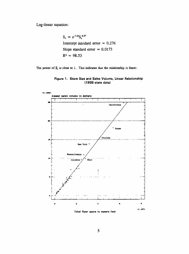
total floor space (SO of supermarkets. A linear equation (Figure 1) fits as well as

log-linear equation (Figure 2)° Sv is measured in dollars and S, is measured in square feet.

Linear equation:

Sv = o54o51 + 0.00037S,

(127.78) (0°0000069)

R= = 98.40

The intercept is insignificant ha this case because the error term of the intercept is much greater thanthe value of intercept.

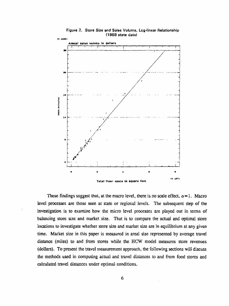
Log-linear equation:

Sv ---- C’7"42Ss0’~

Intercept standard error = 0.276

Slope standard error = 0.0173

R2 = 98.53

The power of S. is close to 1. This indieate~ that the relationship is linear.

Figure 1. Store Size and Sales Volume, Linear Relationship(1988 state data)

AnnuoJ so|cos volume in dollops! ’ ’ ’ Z ’ ’ ’ I , , , [ , , , [

ToLt| floor spice in squore feel

2Q

~S

~e

Store Size and Sales Volume, Logqinear Relationship( 1988 state data)

Annua| sales volume in de||=rs

............... = " ~ ...... " ......................................................

t ~ L I [ i I I [ J [ , I ~ L ~ [

Tots| Neer space in squere feel(x £E~T)

These findings suggest that, at the macro level, there is no scale effect, ~= 1. Macro

level processes are those seen at state or regional levels. The subsequent step of the

investigation is to examine how the micro level processes are played out in terms of

balancing store size and market size. That is to compare the actual and optimal store

locations to investigate whether store size and market size are in equilibrium at any given

time. Market size in this paper is measured in areal size represented by average travel

distance (miles) to and from stores while the HCW model measures store revenues

(dollars). To present the travel measurement approach, the following sections will discuss

the methods used in computing actual and travel distances to and from food stores and

calculated travel distances under optimal conditions.

6

3. Equilibrium of Store Size and Market Size

In this section, we investigated the equilibrating character of store size and market

size by comparing the actual travel distance to and from stores with the calculated distance

under optimal store location. To trace the location behavior of stores, time series data

from 1940 through 1990 on supermarket locations in Seattle were analyzed in five year

increments.

3.1. Actual travel distances

The actual travel distances to and from stores are measured in the northern portion

of Seattle city proper. This area was chosen because its geographic boundaries are well

defined and the settlement patterns are relatively unchanged. The population density of

this area has been constant over the past few decades and there has been little improvement

of transportation services since the early 1960s. Its selection as a study site was to take

advantage of the stability of growth and development, other than transportation that might

affect the location choices of grocery stores.

In computing an actual average travel distance at a given time slice, the conditions

presented in store locations are treated as a set partitioning problem. Since the locations

of stores and the density of population at each time slice are known in this case, the

solutions derived from set partitioning exercises would yield the physical dimensions of

mi~’ket areas from which the miles traveled to and from stores can be computed. In

calculating travel distances between stores and residences, travel distances are assumed to

be equal to the Euclidian distance. To simplify the analysis the network is assumed to be

made up of links between origins, i (households), and destinations, j (stores), although

assumption does not truly replicate urban travel. The formula used in calculating the

actual travel distance to the nearest store is as follows:

7

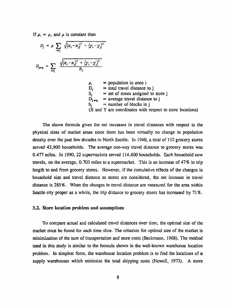
If Pi = P, and p is constant then

Pi

DjSjDjavg

= population in zone i= total travel distance to j= set of zones assigned to store j= average travel distance to j= number of blocks in j

(X and Y are coordinates with respect to store locations)

The above formula gives the net increases in travel distances with respect to the

physical sizes of market areas since there has been virtually no change in population

density over the past few decades in North Seattle. In 1940, a total of 112 grocery stores

served 43,900 households. The average one-way travel distance to grocery stores was

0.477 miles. In 1990, 22 supermarkets served 114,600 households. Each household now

travels, on the average, 0.703 miles to a supermarket. This is an increase of 47% in trip

length to and from grocery stores. However, if the cumulative effects of the changes in

household size and travel distance to stores are considered, the net increase in travel

distance is 285 %. When the changes in travel distance are measured for the area within

Seattle city proper as a whole, the trip distance to grocery stores has increased by 71%.

3.2. Store location problem and assumptions

To compare actual and calculated travel distances over time, the optimal size of the

market must be found for each time slice. The criterion for optimal size of the market is

minimization of the sum of transportation and store costs (Beckmann, 1968). The method

used in this study is similar to the formula shown in the well-known warehouse location

problem. In simplest form, the warehouse location problem is to find the locations of n

supply warehouses which minimize the total shipping costs (Newell, 1973). A more

general formulation is to find n and the location coordinates that minimize the sum of

W, msportation and warehouse costs. One might think that the store location problem is not

quite identical to the warehouse location problem since the cost of transportation in the

warehouse problem is borne by the shipper. Whereas, in the case of the store location

problem, customers pay their own transportation costs. These distinctions, however,

v~ish if the store location problem is treated as a social welfare maximization problem.

In computing the optimal size of food markets, another methodological concern is the

obtainability of the globally optimal spatial patterns of store locations. With the

methodological limitations at hand, the best outcome one could hope for is nearly-optimal

solutions for rigidly specified conditions. Therefore, the formula used in this study is a

solution for a local optimal market size. These methodological limitations are reflected

in the calculated costs considered in the computation of travel distances to and from food

stores. In this study, costs are assumed to be a linear function of distance and the same

for all travellers.

Similar to the warehouse location problem, transportation cost increases with distance

while store cost decreases as store size increases. Thus, the trade-off between

~Lnsportation distances and store sizes is to balance transportation cost and store cost.

The conditions assumed in calculating the optimal market size are:

¯ Total transportation cost is a function of the location of all points, residences and

stores.¯ Cost of stores is a function of store size.¯ Operating cost of stores is a function of sales volume.® Size of store is proportional to the market area served.

,, The location of each store is at the center of its market.

In addition, it is assumed that consumers are utility maximizing individuals whose

objectives are to minimize their total expenditures for any given food purchase° The total

ex]~enditure is the cost of purchasing goods plus the general transportation cost

(expenditures plus travel time cosO. Travel time is assumed to be proportional to distance.

It i.s also assumed that individual customers will patronize a store, say Store I, as long as

9

they believe that the sum of their costs is less than the cost of patronizing Store 2 for

similar goods.

TCI < TC2

tc~ + sol < teq + sea

Where, TCI is total cost to Store 1, TC2 is total cost to Store 2, te~ is transportation

cost to Store 1, te2 is transportation cost to Store 2, se~ is store cost in store 1, and sea is

store cost in store 2. In principle, if scale economies exist, retailers should be able to

offer lower prices for the same goods and to offer a greater variety of choices as stores

grow larger. If the transportation cost is reduced, the opportunity increases for retailers

to expand the size of their stores. The lower the price or the greater the variety of goods,the larger the radius of the market that can be captured. These principles are broadly

interpreted in the formula used in calculating an optimal market size.

Relatively similar size stores serve urban regions regardless of city size even though

there is a strong indication that high density neighborhoods are served by fewer numbers

of stores than low density neighborhoods. To simplify the formula and for the reasons

stated above, the areal size of all Ai are assumed the same and the demand density of all

A~ are equal. Using the above assumptions, the local optimal solution for the market size

of each store was found.

3.3. Method of travel dLC.ance calculation under optimal store location

This section presents the method used in calculating the optimal size of a food

market. The size of a market is defined as the areal size served by an individual

supermarket. As previously stated an optimal market size is the area found by minimizing

the average store cost plus the average cost of transportation. The global minimum cost

can be calculated by integrating over the entire market area.

10

1) Computation of Average Transportation Cost

For simplicity of calculation, the shape of the market is assumed to be circular.

Market areas of different shapes, whether circles, hexagons, triangles, or squares, have

different average travel distances, but the differences are relatively insignificant in travel

distance computation (Newell, 1973). If the ideal shape of a market area is a circle, and

the area A~ is served by a single store which is located at its center, the average travel

di:gtance D.vg for a circular market is 2R/3 where R is radius of a circle. The average

~Lnsportation distance is the total distance divided by the area since we assume that the

density of population is uniform.

The cost of transportation is assumed to be a function of the distance traveled and

proportional to the Euclidean distance of a region (Beckmann, 1968). Thus, the average

transportation cost T.~ per customer for a uniformly distributed demand density for a

circular region, Ai, can be written as:

Tar, = D,vg t= 2Rt/3

= 0.376 tAi~

In this study, t represents the gasoline cost per mile. Gasoline cost is considered

instead of the owning and operating costs of automobiles because we are mostly concerned

with marginal changes in transportation cost. During the last 20 years, automobiles have

become smaller and the efficiency in gasoline mileage has increased. The efficiency in

gasoline mileage was considered in the computation of the average transportation costs.

While the size of households has been decreasing, the number of automobiles per

household has been increasing. This is mainly because more women have access to

automobiles. Over the same period of time, the marginal cost of gasoline has been

decreasing. The decreased marginal cost of gasoline plus the ready availability of

automobiles has resulted in increased demand for urban highways and arterials.

11

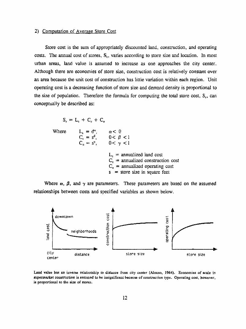
2) Computation of Average Store Cost

Store cost is the sum of appropriately discounted land, construction, and operating

costs. The annual cost of stores, So, varies according to store size and location. In most

urban areas, land value is assumed to increase as one approaches the city center.

Although there are economies of store size, construction cost is relatively constant over

an area because the unit cost of construction has little variation within each region. Unit

operating cost is a decreasing function of store size and demand density is proportional to

the size of population. Therefore the formula for computing the total store cost, So, can

conceptually be described as:

So = L¢ + Cc + Co

Where Lc=d=, c~< 0Cc=s~, 0<B <1Co= s’, 0< 3’ <1

L¢ = annualized land costC~ = annualized construction costCo = annualized operating costs = store size in square feet

Where o~, t, and 3’ are parameters. These parameters are based on the assumed

relationships between costs and specified variables as shown below,

downtown Q

O.to

neighborhoods

t-O

tit’center

f-

O~0t#

e~O

v v v

distance store size store size

Land value has an inverse relationship to distance from city center (Alonso, 1964). Economies of scale supermarket construction is assumed to be insignificant because of construction type. Operating cost, however,is proportional to the size of stores.

12

As is true of most urban areas, until the 1960s there was a bountiful supply of

cx~mmercially zoned properties along major arterials. Land for possible sites for

supermarket development was found in all areas of Seattle residential neighborhoods. The

land price between commercial and residential uses varied significantly but land price

within neighborhood commercial zones did not vary much. Supermarkets during the study

period were located in the outer ring of the urban center, mostly in residential

neighborhoods. For this reason, only operating cost is considered in the store cost

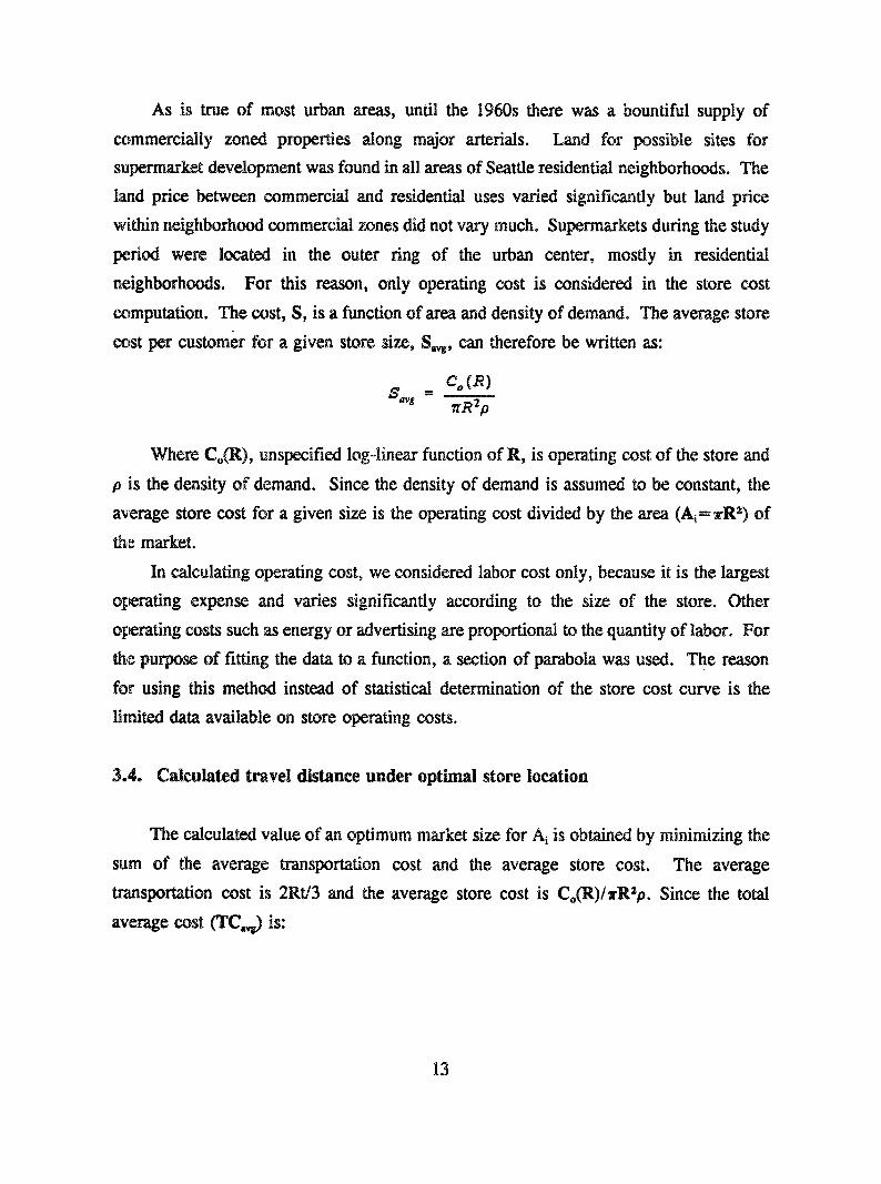
computation. The cost, S, is a function of area and density of demand. The average store

cost per customer for a given store size, S~,,, can therefore be written as:

s,~- co(R)~R2p

Where Co(R), unspecified log-linear function of R, is operating cost of the store and

p is the density of demand. Since the density of demand is assumed to be constant, the

average store cost for a given size is the operating cost divided by the area (Ai = ~-R’)

the market.

In calculating operating cost, we considered labor cost only, because it is the largest

operating expense and varies significantly according to the size of the store. Other

operating costs such as energy or advertising are proportional to the quantity of labor. For

the purpose of fitting the data to a function, a section of parabola was used. The reason

for using this method instead of statistical determination of the store cost curve is the

1/miter data available on store operating costs.

3.,4. Calculated travel distance under optimal store location

The calculated value of an optimum market size for Ai is obtained by minimizing the

sum of the average transportation cost and the average store cost. The average

~msportation cost is 2Rt/3 and the average store cost is Co(R)/~-R=p. Since the total

average cost (TCo,,) is:

13

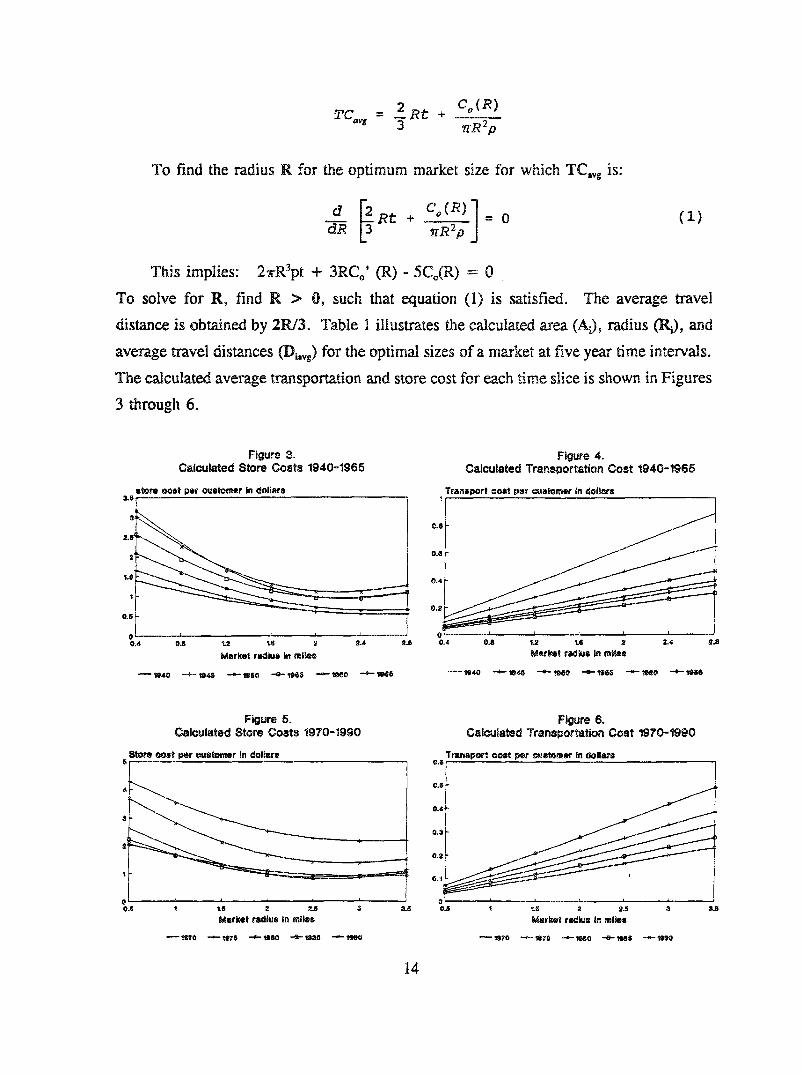
TCav ~ = 2 Rt ÷ Co(R)3 ~R 2p

To find the radius R for the optimum market size for which TC,,~ is:

(i)

This implies: 27rR3pt + 3RCo’ (R) - 5Co(R)

To solve for R, find R > 0, such that equation (1) is satisfied. The average travel

distance is obtained by 2R/3. Table 1 illustrates the caJculated area (A0, radius 0~., and

average travel distances (D,.vg) for the optimal sizes of a market at five year time intervals.

The calculated average transportation and store cost for each time slice is shown in Figures

3 through 6.

Figure 3.Calculated Store Costs 1940-1965

afore oost per ou=tocrmr In dollars3.6

2;

LS=

2~

1.6"

1

0.6

G.4i i , i i

Q~ %2 %8 2 2.4 2.6

Market racllu- |n mils

Figure 4.Calculated Transport=tion Cost 1940-1965

Traneport oost per customer In ¢~olP=r=1

0.8

0.0

0.4

0.2

O= I0.4 0.8 %6 2 2.4 2.8

Marko! radius ~n m~tee

Figure 5.Calculated Store Costs 1970-1990

Store oost per ouetomer in dollare5

0OJS

i i i iI %0 2 2.5 3

M=rke¢ radius in milee

Figure 6.Calculated Transportation Cost 1970-1990

Tmneport ooet pot ~etoms~ in dollars

1oi,f

6J~ ~ %~ 2 ~.5 3 3.~

Market radius In milee

197G -+- ~72 "=~ I~0 ~ ?~1~ ~

14

3.5. Comparison between actual and calculated travel distances

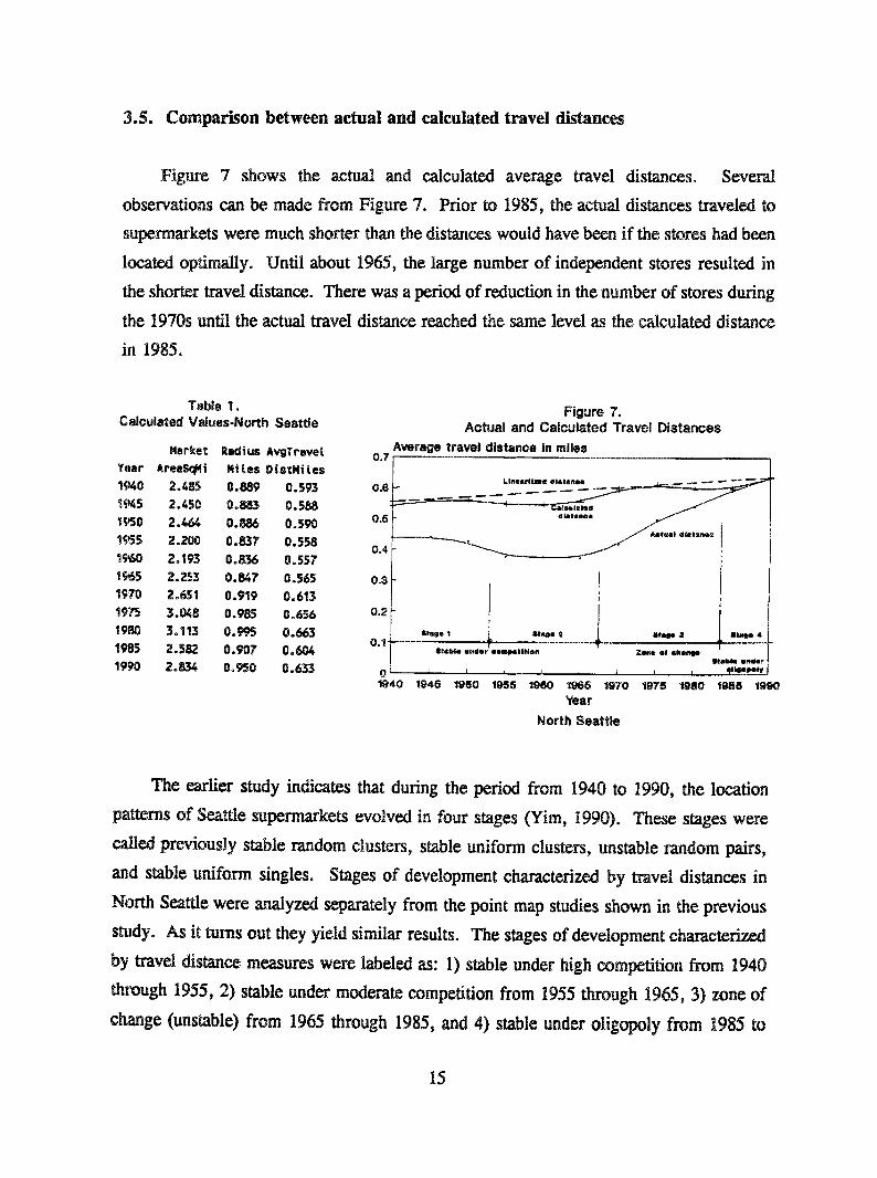
Figure 7 shows the actual and calculated average travel distances. Several

observations can be made from Figure 7. Prior to 1985, the actual distances traveled to

~upermarkets were much shorter than the distances would have been if the stores had been

located optimally. Until about 1965, the large number of independent stores resulted in

the shorter travel distance. There was a period of reduction in the number of stores during

the 1970s until the actual travel distance reached the same level as the calculated distance

in 1985.

Table 1.CaJculated Values-North Seattle

Market Rodius AvgTrmvelYear AreaS~| Mites OistMites1~0 2.485 0.889 0.593~945 2.450 0.88:3 0.588~50 2./~ 0.886 0.5901~55 2.200 0.837 0.5581;~0 2.193 0.836 0.557~9~5 2.253 0.847 0.56519’70 2.651 0.919 0.6’131975 3.0~8 0.985 0.6561980 3.113 0.995 0.6631985 2.582 0.907 0.6041990 2.~T~ 0.950 0.633

Figure 7.Actual and Calculated Travel Distances

Average travel distance in miles

..... --,--°.°to2r=

°:t1940

North Seattle

The earlier study indicates that during the period from 1940 to 1990, the location

patterns of Seattle supermarkets evolved in four stages (Yim, 1990). These stages were

called previously stable random clusters, stable uniform clusters, unstable random pairs,

and stable uniform singles. Stages of development characterized by travel distances in

North Seattle were analyzed separately from the point map studies shown in the previous

study. As it turns out they yield similar results. The stages of development characterized

by travel distance measures were labeled as: 1) stable under high competition from 1940

through 1955, 2) stable under moderate competition from 1955 through 1965, 3) zone

change (unstable) from 1965 through 1985, and 4) stable under oligopoly from 1985

15

1990. Travel distance is market size related and market size is presumed to be determined

by spatial competition. In the early stage of development, many independent firms created

a highly competitive market. The higher the competition the smaller the size of each

market and, consequently, the shorter the distance that consumers had to travel. However,

as shown in Figure 7 the trend is now moving toward one supplier dominating the market.

In Seattle, this supplier is Safeway.

4. Rate of Change in Store Locations

Attention is now directed to the rate of change in store locations. That is, how

frequently have supermarket locations changed in Seattle over the past 50 years and what

are the factors influencing the location choice of grocery stores? The rate of change in

store locations is measured in two ways: the longevity of store locations and the survival

rate of stores. This analysis is toward understanding the extent to which the travel patterns

of food shopping are affected by the survival rate of food stores and the longevity of store

locations.

4.1. Overview of food retail locations

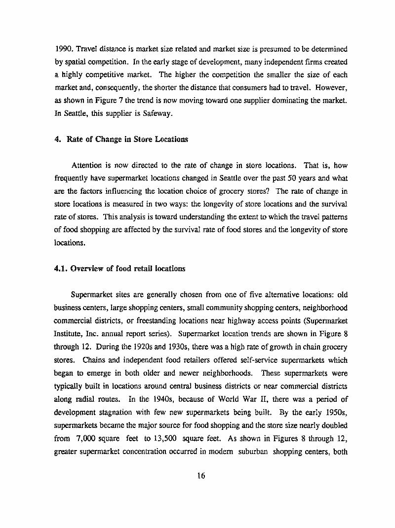
Supermarket sites are generally chosen from one of five alternative locations: old

business centers, large shopping centers, small community shopping centers, neighborhood

commercial districts, or freestanding locations near highway access points (Supermarket

Institute, Inc. annual report series). Supermarket location trends are shown in Figure

through 12. During the 1920s and 1930s, there was a high rate of growth in chain grocery

stores. Chains and independent food retailers offered self-service supermarkets which

began to emerge in both older and newer neighborhoods. These supermarkets were

typically built in locations around central business districts or near commercial districts

along radial routes. In the 1940s, because of World War II, there was a period of

development stagnation with few new supermarkets being built. By the early 1950s,

supermarkets became the major source for food shopping and the store size nearly doubled

from 7,000 square feet to 13,500 square feet. As shown in Figures 8 through 12,

greater supermarket concentration occurred in modem suburban shopping centers, both

16

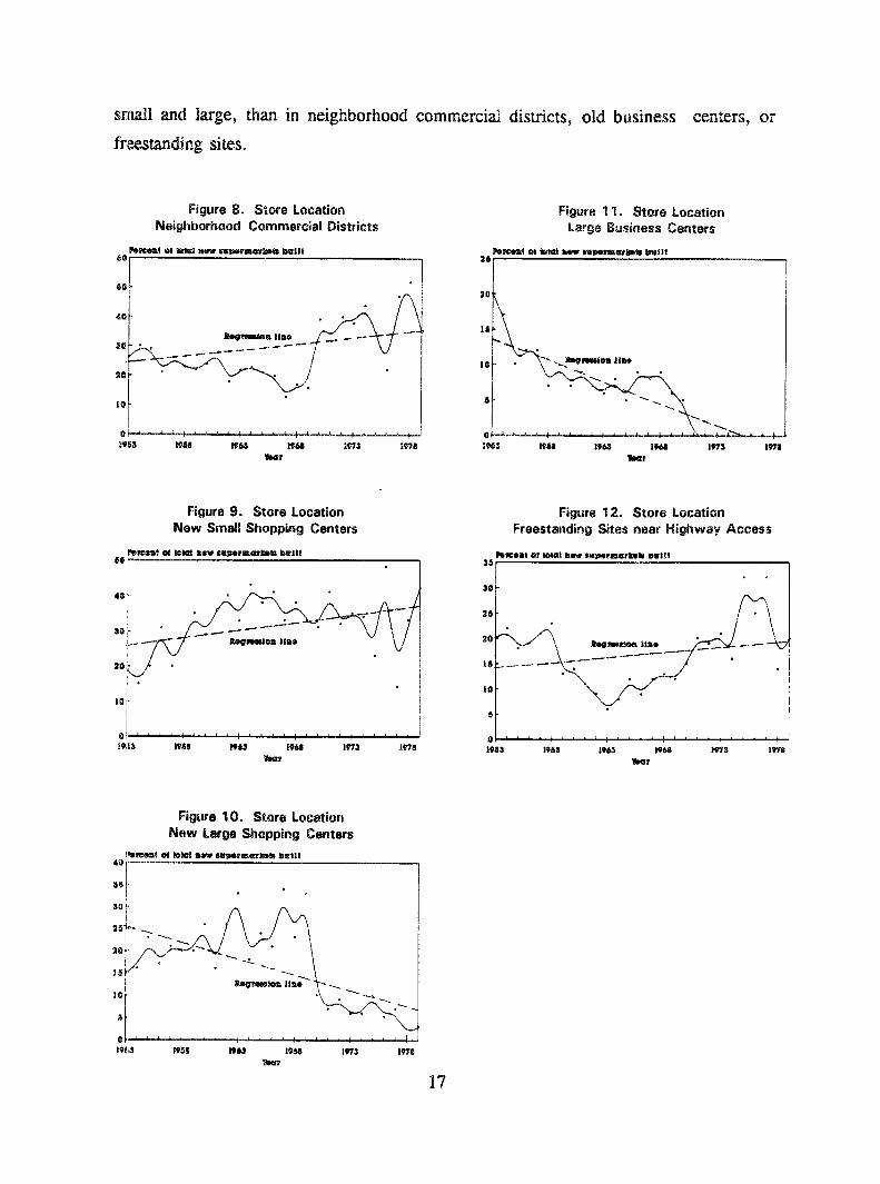
sraall and large, than in neighborhood commercial districts, old business centers, or

freestanding sites.

Figure 8. S~ore LocationNeighborhood Commercial Districts

Figure 11. Stme LocationLarge Business Centers

I0

6

0|965

Figure 9. Store LocationNew Small Shopping Centers

Figure 120 Store LocationFreestanding Sites near Highway Access

1958 1963 19611 |973 1978Ys~r

Figure 10. Store LocationNew Large Shopping Centers

|+l~®=it Of kHal I~e~+ 801~11’l~Otl~lll bt~lll

17

During the 1960s, supermarkets became even larger, especially the ones in suburban

communities. More than half of all new supermarkets (65%) were located in shopping

centers. Small shopping centers gained a considerably higher number of supermarkets

(40% of the new supermarkets built) than the large shopping centers (25 %). The percent

of new supermarkets built in neighborhood commercial districts remained the same but the

percent of new supermarkets in old business centers and freestanding sites was

significantly reduced.

The trend in the 1970s and I980s was toward locating supermarkets in neighborhood

commercial districts or small community shopping centers. Nearly 40% of new

supermarkets chose neighborhood commercial districts and 35 % chose small community

shopping centers. Very few new supermarkets were built in old business centers or large

shopping centers. Freestanding sites, however, became popular, mainly because of the

availability of land.

In the I990s, the trend to larger stores may continue along two basic paths. One is

toward even larger supermarkets or superstores typically located in community-scale

shopping centers adjacent to large drug and variety stores. The other path is toward

ultra-large bulk discount stores (the warehouse type) developing in suburban areas around

central cities. These bulk stores are currently locating on major urban arterials or near

freeway access points serving regional scale markets. Only a few of these extra large

stores are needed to serve an entire metropolitan area.

If bulk discounters continue to expand their share of the market, the conventional

supermarkets will have to change. Since conventional supermarkets cannot compete in

price, they will have to compete in other areas such as service and convenience --

qualities the bulk discounters have difficulty offering. Supermarkets may become more

like large ’convenience’ markets as they expand their ready-to-eat deli bars and exotic

foods departments, acknowledging that the bulk discounters are taking away portions of

their market share (Progressive Grocer, 1989).

4.2. Choice of store locations

As Nelson (1958) and Applebaum (1968) noted, retail business locations are

market oriented, and they are thus governed by accessibility to customers. Nelson and

18

Applebaum’s studies of supermarket locations indicated that food markets are "generative"

types. This means that store locations are strongly governed by the location of residential

neighborhoods and that they provide goods and services that attract consumers. Grocers

~rely make location decisions based solely on the "suscipient" type market attraction.

Su.scipient type shopping occurs when customers are "impulsively or coincidentaUy

atWacted while moving about the area where the retail store is located." (Applebaum,

1968.)

As Applebaum also noted, the value of a store location depends on three factors:

I) accessibility to residences and to people moving about, 2) physical attributes,

including araple parking and safe environment, and 3) good will or store reputation.

Nelson (1958) stated, "Each retailer chooses store location based on the productivity

the location relating to its potential ability to yield maximum profit." He suggested that

food retailers must be aware of the following critical points in store location:

1) The market potential of the store location based on the sales volume and capturerate of the existing and future market in order to determine the risk factors ofsuccess, for example, whether food stores are over-or under-supplied prior toentering the market.

2) The market area’s growth potential in terms of the consumer population. This ismore applicable to the expanding suburbs than to the already built-up urbanneighborhoods.

3) The physical accessibility to a trade area for self-sufficiency and for support fromother neighboring businesses. The latter assists in extending a store’s drawingpower beyond the local trade area. It is better for food stores to be located withcomplementary stores than with similar ones.

4) The business intercept by locating stores between residences and the existing storeswhere people regularly shop for their groceries. In the same vein, retailers shouldavoid sites vulnerable to business intercept. Food stores, however, do not onlycompete with their locations but also with their prices arid the quality of theirservice.

Relail experts regard the turn-over rate in supermarket locations as extremely high

compared to comparison goods stores.

19

4.3. Distribution of supermarkets, chains vs independent stores

The analyses to be reported now are tests of a series of hypotheses with respect to

the life cycle of supermarkets in Seattle. Our conjecture is that between stores and

markets, balance is established by way of spatial competition. The null hypothesis, in a

broad sense, is that changes in store locations are simply a result of birth and death

processes that are driven by the random chance events of success and failure in a

competitive market. The motivation behind the investigation of this hypothesis is to shed

light on what seems to be the actual processes that take place in balancing store size and

market size in competition. This section, therefore, examines whether the number of

stores entering or leaving the market have proportional relationships to 1) existing

supermarket populations or 2) the number of births or deaths of supermarkets at any given

time.

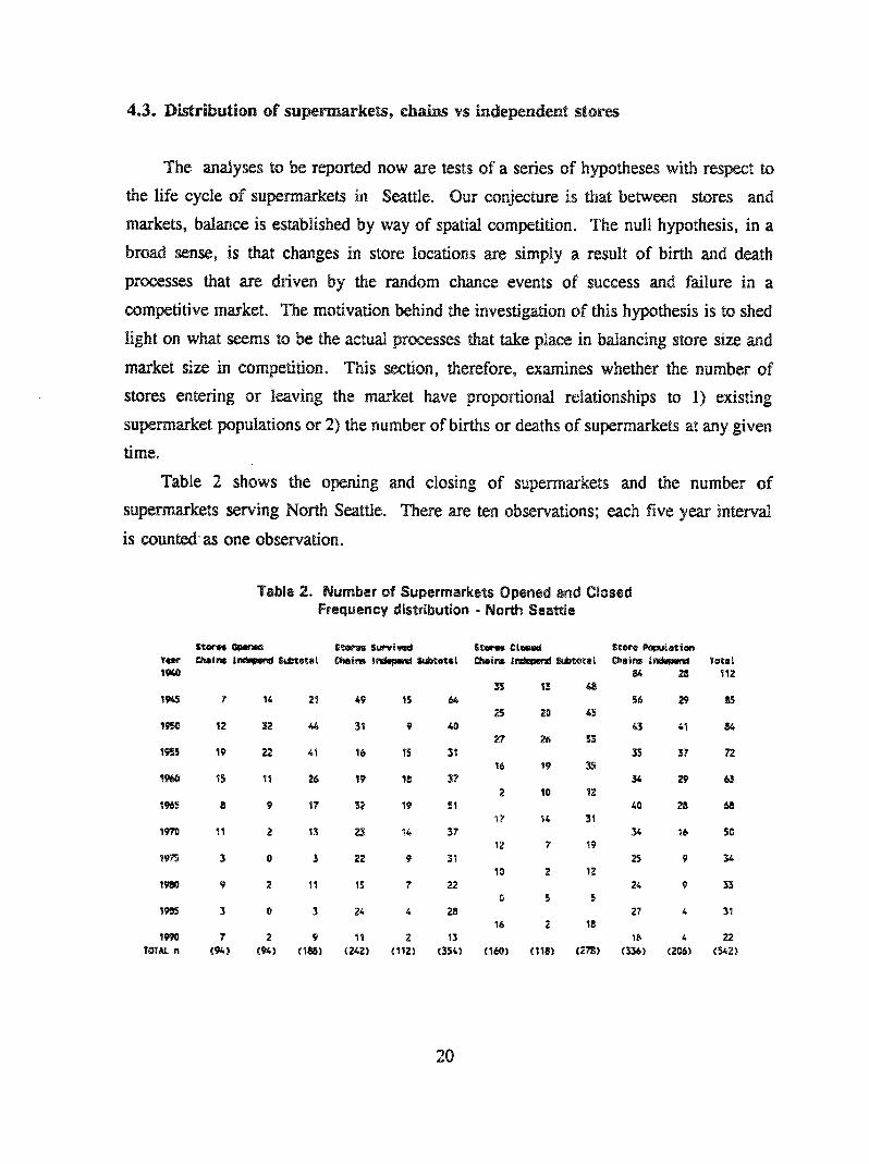
Table 2 shows the opening and closing of supermarkets and the number of

supermarkets serving North Seattle. There are ten observations; each five year interval

is counted as one observation.

Table 2. Number of Supermarkets Opened and ClosedFrequency distribution - North Sea~Je

Stocks Oper~ S~wes Suryi~cl $to¢’es Cta~a

35 131~5 7 14 21 49 I5

25 20 451~0 12 32 44 31 9 40

;~7 26 531955 19 Z2 41 16 15 31

16 19 3S1960 t5 11 ~6 19 18 37

2 10 I21965 8 9 17 32 19 51

17 14 311970 11 2 13 23 14 37

12 7 191975 3 0 3 Z2 9 3~

1o 2 121980 9 2 11 15 7 22

0 5 SI~5 3 0 3 24 4 28

16 ;~ 181990 7 2 9 I1 2 13

TOTAL n (94) (94) (188) (242) (112) (35/*) C160) Cl18~ (278)

2O

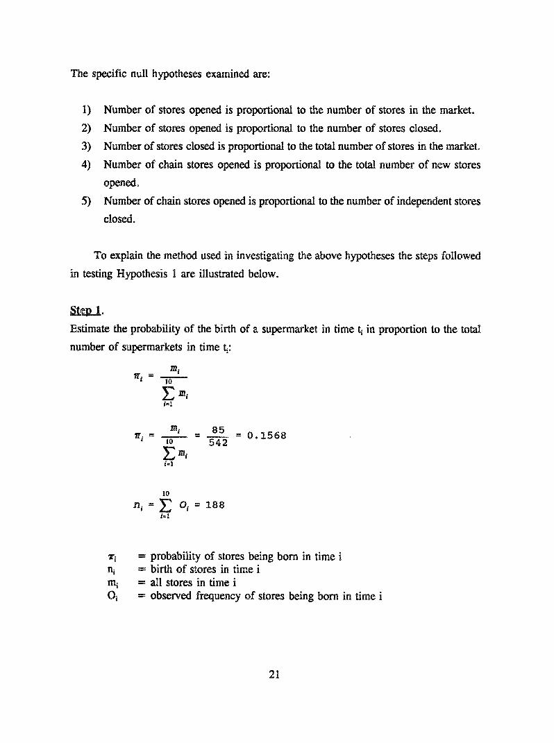
The specific null hypotheses examined are:

1) Number of stores opened is proportional to the number of stores in the market.

2) Number of stores opened is proportional to the number of stores closed.

3) Number of stores closed is proportional to the total number of stores in the market.

4) Number of chain stores opened is proportional to the total number of new stores

opened.

5) Number of chain stores opened is proportional to the number of independent stores

closed.

To explain the method used in investigating the above hypotheses the steps followed

in testing Hypothesis 1 are illustrated below.

st,m_!.Estimate the probability of the birth of a supermarket in time % in proportion to the total

number of supermarkets in time %:

miHi = 10

mji-|

m~ 85~’i = - = O. 1568lo 542

Emi

ni

1o

= E Oi = 188iffil

= probability of stores being born in time i= birth of stores in time i= all stores in time i= observed frequency of stores being born in time i

21

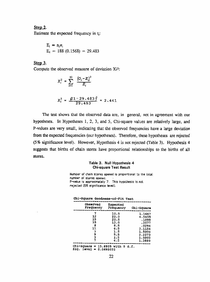
Step 2.Estimate the expected frequency in %:

El = ni"//’i

El = 188 (0.1568) = 29.483

Compute the observed measure of deviation Xi2:

The test shows that the observed data are, in general~ not in agreement with our

hypotheses. In Hypotheses 1, 2, 3, and 5, Chi-square values are relatively large, and

P-values are very small, indicating that the observed frequencies have a large deviation

from the expected frequencies (our hypotheses). Therefore, these hypotheses are rejected

(5 % significance level). However, Hypothesis 4 is not rejected (Table 3). Hypothesis

suggests that births of chain stores have proportional relationships to the births of all

stores.

Table 3. Null Hypothesis 4Chi-square Test Result

Number of chain slopes opened is peoooetionsI Lo the totalnumber of st, oces opened.P-value is approximaLety 7. This hypothesis is noLrejecLed (SR significance level).

C.hi-Square Goodness-of-Fit Test

Observed ExpectedFrequency Frequency Phi-Square

7 10.5 1.166712 22.0 4.545519 20.5 ,I09815 13.0 .3077

8 8.5 00294ii 6.5 3.1154

3 1.5 1.50009 5.5 2.22733 1.5 1o50007 4.5 1.3889

Chi-square = 15.8905 with 9 d.f.Sig. level = 0.0692032

22

From this analysis the following observations are made:

1) Considering long-run effects, the hypotheses of the proportional relationships

generally do not hold. Food stores entering the market do not necessarily depend on the

number of competing stores in the market. This suggests that the relationship is more

complex than postulated. A possible reason for this is that the decision to enter the market

is governed by many factors beyond spatial competition. Among these factors are

ch~nges in the local and national economies and disposable income. As shown in Table

2, the local economy is strongly reflected in the number of stores opened and closed in the

post-war era as well as during the Seattle recession in the early 1970s when Boeing had

a massive layoff. Between 1950 and 1960, the number of new stores opened averaged

about forty stores per year. Stores closed during that time were about the same number.

In 1975, there were only three stores opened but twelve stores closed.

Another factor, the life-cycle of stores, is significantly influenced by the emergence

of modernized supermarkets and the high rate of growth in store size. Introduction of new

types of grocery stores caused the stores to either expand on existing sites or to find new

locations for large store sites. The high turn-over rate in supermarket locations could

have been due to the replacement of many small old supermarkets with a few large modern

superstores.

2) It is reasonable to assume that chain supermarkets enter a market in proportion to the

totad supermarkets opened. Any deviation shown between the observed frequency and the

exr~cted frequency is due to chance. Thus, the supermarket population may have been

influenced largely by the behavior of chain stores.

3) Chain stores have increasingly dominated the market. The investigation of

Hypothesis 5, that the opening of chain stores is proportional to the closing of independent

stores, supports this observation. Although a fair number of chain stores were closed over

the years, it appears that chains are taking over the entire food market in Seattle. See

Table 2, the column showing the total store population.

23

4.4. Survival times and longevity of store locations

This section addresses several questions related to store location patterns: to

what extent are patterns of store locations dependent on historical paths? If location

choices were made differently along the way, would the patterns have developed

differently? Such questions are typically raised in industrial location and logistics

literature. An example is the recent study by Arthur (1988) who asked, "could different

’chance events’ in history have created a different formation of urban centers than the one

that exists today," or do "the patterns of industry location follow paths that depend on

history’? In his view, spatial patterns of industry locations are determined by "a mixture

of economic determinism and historical chance -- and not [by] either alone." Patterns of

urban activities cannot be explained or predicted without knowing what historical events

have occurred. Arthur defines these as chance events, coincidences, and circumstances.

It seems likely that patterns of store locations are also determined by both historical chance

and economic determinants.

Within this context two aspects of store locations are examined from a historical

perspective. One is survival times of supermarkets with respect to ownership, chains

versus independent stores° The second is survival times of supermarkets with respect to

the characteristics of store sites, old sites versus new sites. Old sites are defined as sites

previously used for food retailing or sites that are within approximately a one block radius

thereof. New sites are defined as locations where food stores are freestanding and where

no food retailing has existed previously.

1) Survival Time of Food Stores

The longevity of food stores in Seattle will now be discussed in terms of ownership,

chains versus independents° What is the expected life-span of food stores in general and

are chains able to survive longer than independent stores? The purpose of this investigation

is to identify the length of time that stores survived during the study period from 1945

through 1985. Survival time is defined as the time from initial observation until failure.

Failure is defined as the store’s permanent closure.

For this analysis, survival time is grouped into five year fixed intervals. The

24

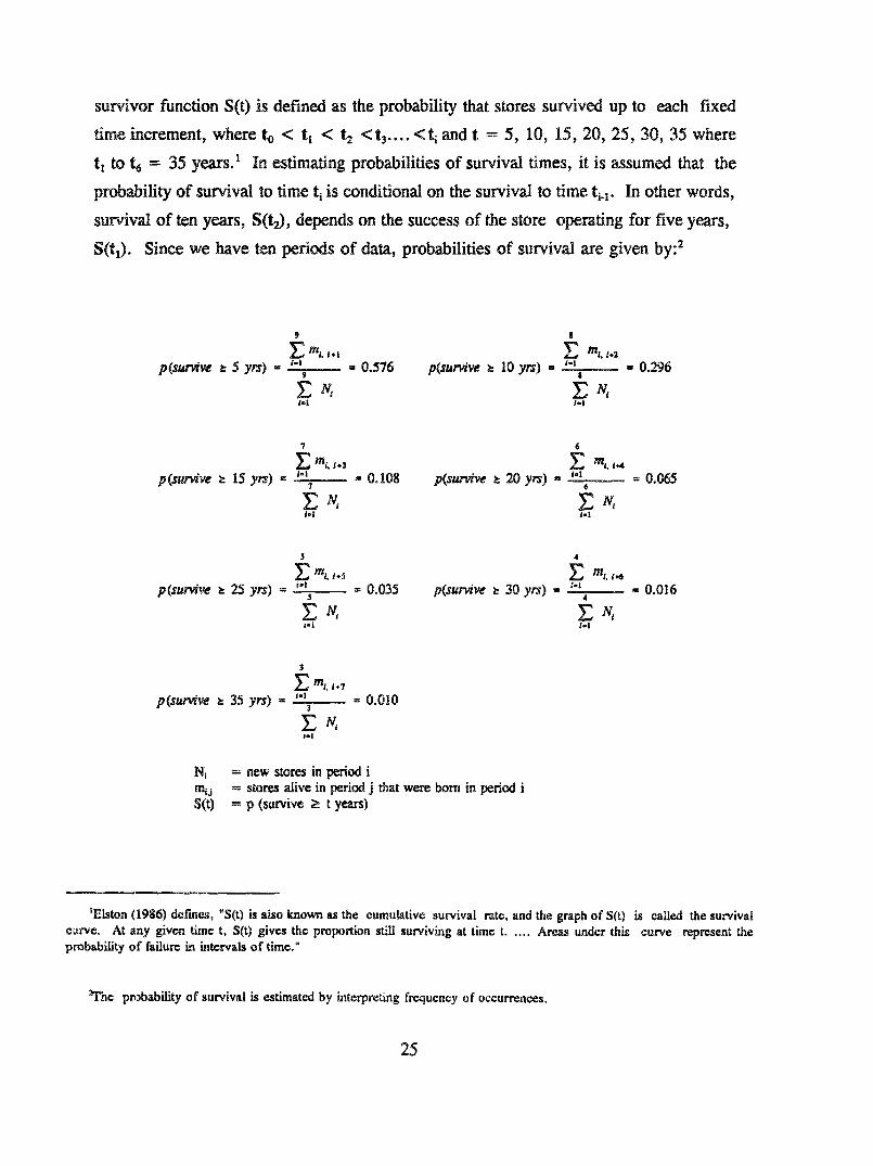
survivor function S(t) is defined as the probability that stores survived up to each fixed

time increment, where to < tt < t2 <t3 .... <ti and t = 5, 10, 15, 20, 25, 30, 35 where

tt to t~ = 35 years.1 In estimating probabilities of survival times, it is assumed that the

probability of survival to time ti is conditional on the survival to time t~. In other words,

surviival of ten years, S(tz), depends on the success of the store operating for five years,

S(tl). Since we have ten periods of data, probabilities of survival are given by:2

p(survive ~ 5 yrs) ,, = 0.296

0.108 p(survive ~ 20 yrs) - 0.065

= 0.035 p(survive ~. 30 yrs) -- - 0.016

p(su~ve ~ 35 yrs) = -- - 0.010

Ni = new stores in period imij = stores alive in period j that were born in period i$(t) = p (survive ~ t years)

IElston (1986) defines, "S(t) is also known as the cumulative survival rate, and the graph of S(t) is called the survivalcurve. At any given time t, S(t) gives the proportion still surviving at time t ..... Areas under this curve represent theprobability of failure in intervals of time."

~rhe pr~)bability of survival is estimated by interpreting frequency of occurrences.

25

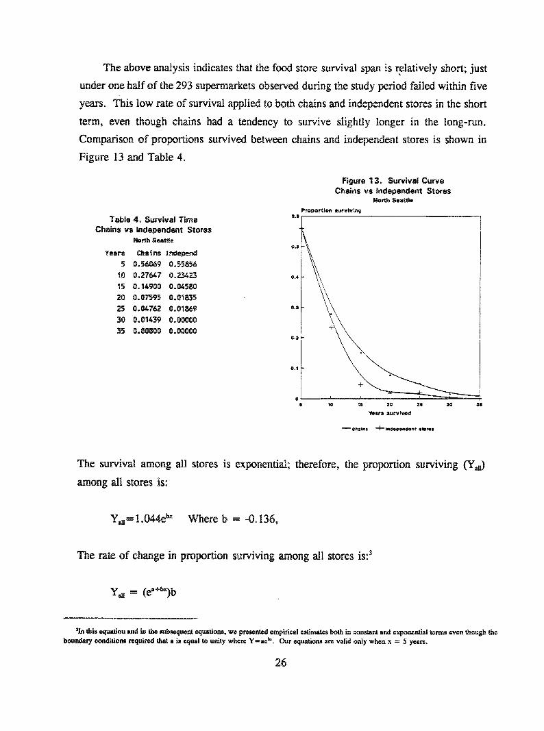
The above analysis indicates that the food store survival span is relatively short; just

under one half of the 293 supermarkets observed during the study period failed within fiveyears. This low rote of survival applied to both chains and independent stores in the short

term, even though chains had a tendency to survive slightly longer in the long-run.

Comparison of proportions survived between chains and independent stores is shown in

Figure 13 and Table 4.

TebJe 4o Survival TimeChains vs Independent Stores

Nollh 8eatl~

Years Cheins I ndepend5 0.56069 0.55856

10 0.27(~7 0.2342315 0.14900 0.0458020 0.07595 0.0183525 0.04762 0.01~6930 0.01439 O.O000O35 0.00800 0.00000

Figure 13. Survival CurveChains vs Independent Stores

North Seattte

Proportion euevlvl~0.$

o., \)~\

!

The survival among al! stores is exponential; therefore, the proportion surviving (YJ

among all stores is:

Y~= 1.044eb~ Where b = -0.136,

The rate of change in proportion surviving among all stores is:3

Sin this equation and in the mbsequent eqtmtions, we presented empirical estimates both in eom~ant ~nd exponential terms even though theboundary eonditiorm requited that aie eXlU~l to uni~y where Y--ae~. Our equations are valid only when x -- 5 years.

26

T, he changes in proportion surviving (aY,) after n years since year x is:

Vv~lere aebx is the number of beginning stores in time x, ae~x÷n~ is the number of stores

remaining after n years since time x, and (1-ae~) is the percent of remaining stores lost

in n year. The survival curves among chains and independent stores axe also exponential.

Tlle proportion surviving (Yo "t~) among chains is:

Yo~ = 0.922ebx Where b =-0.082

The proportion surviving (Y,~t) among independent stores is:

Y~ = 0.855eb~ Where b =-0.277

The high values of R2 indicate that exponential models fit food store survival curves very

weU.

2) Success and Failure of Store Locations

This section reports on the analysis of the survival times of store locations between

old sites and new freestanding sites. The questions are: do stores choosing old sites have

a tdgher success rate than those choosing freestanding sites and how frequently do stores

see, k new freestanding sites?

The analysis indicates that stores choosing freestanding sites have a slightly higher

probability of surviving longer than the stores choosing old sites. The analysis shows that

52 % of new store sites and 47% of old store sites are expected to survive more than five

ye~trs. Seventeen percent of new store sites and 15 % of old sites are expected to survive

more than ten years. Comparison of the proportion of successes to failures among the old

and new sites is shown in Figure 14 and Table 5.

27

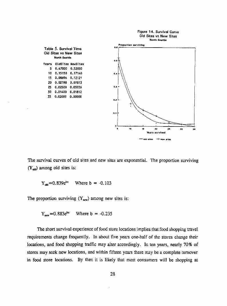
Table 5. Survival TimeOld Sites vs New Sites

Noah Seat~

Years OtdSJtes NewSites5 0.47000 0.52000

10 0.15150 0.1714015 0.08696 0.12121

20 0.02198 0.0~’13

25 0.02500 0.0322630 0.01400 0.01812

35 0.02000 0.00000

0.0

0.3

0.2

The survival curves of old sites and new sites are exponential. The proportion surviving

Cg,,k~) among old sites is:

Yo~=0.839e~ Where b = -0.103

The proportion surviving (Yn~,,) among new sites is:

Y~=0.883ebx Where b = -0.235

The short survival experience of food store locations implies that food shopping travel

requirements change frequently. In about five years one-half of the stores change their

locations, and food shopping traffic may alter accordingly. In ten years, nearly 70% of

stores may seek new locations, and within fifteen years there may be a complete turnover

in food store locations. By then it is likely that most consumers will be shopping at

28

different store locations which will undoubtedly create new travel patterns for food

shopping.

S. Summary and Conclusions

From this study, several conclusions can be reached: first, the total floor space of

food stores is strongly correlated to market size measured in sales volume when the data

aggregated at the state level are examined. Second, for many years, the actual average

~wel distances in Seattle to and from supermarkets were shorter than the transportation

di:stances calculated under the optimal size of market. However, the actual average travel

distance and the calculated average distance converged around the mid-1980s which

indicates that an equilibrium was reached at that point. This convergence suggests that

current food stores are located optimally. Third, using the travel distance measure, the

study found that there were four distinctively different grocery shopping travel patterns in

Seattle over the past 50 years. This finding concurs with the earlier study done with the

location patterns of supermarkets in Seattle (Yim, 1990).

Fourth, spatial competition was presumed to be a benchmark for the measure of store

location behavior, that is the movement toward a spatial equilibrium. However, a series

of hypotheses tested indicates that the choice of a store entering the market is governed

by factors other than spatial competition. These factors include the state of the local

economy and the introduction of new store types. As mentioned earlier, food stores have

ew3lved from superettes to superstores over the past several decades. This transformation

process required ever-increasing store size and, as a result, there was a high turnover in

food store locations.

Finally, the life span of supermarkets in Seattle was fairly short compared to other

types of urban activities. Nearly 50% of the supermarkets failed within five years and

over 80% failed within ten years. This rate applied to both chains and independent stores.

Stores on freestanding sites showed a slightly higher probability of surviving longer than

stores on old sites. The short survival span in store locations suggests that grocery

shopping travel patterns may be altered significantly in the future.

The merit of this research lies in its approach toward an understanding of urban

systems, the process of change with respect to scale and scope, location, life cycle,

29

mutation, and environment. In other words, this research was aimed at expanding our

knowledge of the evolutionary process of urban activities as it relates to transportation

requirements. In this study our research was restricted to transportation and retail

activities. On a broad spectrum, a research topic deserving attention is the cumulative

effects of transportation services on the entire food sector, including truck and rail

transportation impacts on the productivity of the retail and wholesale food markets. For

example, employment in farming, forestry, and fishing declined from 4.7% in 1972 to

3.1% in 1986 while technical, sales, and administrative support gained from 28.8% in

1972 to 31.3 % in 1986 respectively (Congress of the United States, Office of Technology

Assessment, 1988). The question is how does the whole span of transportation technology

affect the shifts in the employment sectors of the food industry? There are also

improvements to be made in the methodological aspects of this paper. For example, we

used Euclidian distance in measuring travel distances to and from stores. This may not

matter if only changes in relative travel distance are measured, but if quantitative measures

of traffic diversions on networks are to be obtained, the block distance measurements

would be more useful.

The findings of the study suggest that the relation of transportation services to retail

activities is not a straightforward one. It is a complex relationship and involves the

evolution of technology. Changes in technology regimes provide opportunities for

innovation in production and marketing. This neo-Schumpeterian view of the process of

change makes urban systems complex and difficult to model (Nelson and Winter, 1982).

As a result, this paper opens up many puzzles. Further studies in this general area will

provide opportunities to obtain deeper understanding of the relationship of transportation

to the behavior of urban retail activities.

30

References

Alle~a, Peter M., Self-Organization in Human Systems; Essays in Societal System Dynamics andTransportation, Report no. DOT-TSC-RSPA-81-3, Research and Special Programs Admin-istration, Washington DC, March 1981.

Allen, P.M. et al., Models of Settlement and Structure as Dynamic Self-Organizing Systems,Report no. DOT-TSC-1640 Research and Special Programs Administration, Washington DC,February 1981.

Alonso, W., Location and Land U~e, Harvard University Press, Cambridge, MA, 1964.

Applebaum, William, Guide to Store Location Research with Emphasis on Super Markets~Super Market Institute, Inc., Addison-Wesley, Reading, MA, 1968.

Arthur, Brian W., "Urban Systems and Historical Path Dependence," City and Their VitalSystems: Infrastructure Past. Present and Future, eds. Jesse H. Ausubel and Robert Heman,Natural Academy Press, Washington DC, 1988.

Beaumont, J., M. Clarke, P. Keys, H. Williams and A. Wilson, "The Dynamical Analysis ofUrban Systems: An Overview of On-Going Work at l.eexis," Essays in Societal SystemD~mics and Transportation, Report no. DOT-TSC-RSPA-81-3, Research and SpecialPrograms Administration, Washington DC, 1981.

Beckmann, Martin, Loc~, Random House, New York, 1968.

Congress of the United States, Office of Technology Assessment, Technology and the AmericanEconomic Transition. Choice for the Future, Washington DC, May 1988.

Harris, B., Choukroun, J.M. and Wilson, A.G., "Economies of Scale and the Existence ofSupply-side Equilibria in a Production-constrained Spatial-interaction Model," Environment andPlanning A, 14, 823-837, 1982.

Nelscm, R.L., The Selection of Retail Locations, F.W. Dodge, New York, 1958.

Nel~xm, Richard R. and Winter, Sydeny G., An Ev01ution~_ry Theory_ of Economic Change, TheBelknap Press of Harvard University Press, Cambridge, MA, 1982.

Newell G. F., "Scheduling, Location, Transportation, and Continuum Mechanics; Some SimpleApproximations to Optimization Problems," SIAM Journal on Applied Mathematics, 25(3),346-3,60, November 1973.

31

Progressive Grocers, Maclean Hunter Media, Stamford, CT, 1976 -1989.

Yim, Youngbin, "Travel Distance and Market Size in Food Retailing," The University ofCalifornia Transportation Center, Working Paper UCTC No. 124, Berkeley, CA, 1990.

32