JUNTA DE ENERGÍA NUCLEAR - IPEN · y Publicaciones, Junta de Energía Nuclear, Ciudad Uni-versitaria, Madrid-3, ESPAÑA. Las solicitudes de ejemplares deben dirigirse a este mismo

J.E.N.448Sp ISSN 0081-3397

The neutrón transport code DTF*-Tracauserfs manual and input dataD

by

AHNERT, C.

JUNTA DE ENERGÍA NUCLEAR

CLASIFICACIÓN INIS Y DESCRIPTORES

E21D CODESMANUALSNEUTRÓNTRANSPORTDISCRETE ORDINATE METHODONE DIMENSIONAL CALCULATIONSNEUTRÓN TRANSPORT THEORY

Toda correspondencia en relación con este traba-jo debe dirigirse al Servicio de Documentación Bibliotecay Publicaciones, Junta de Energía Nuclear, Ciudad Uni-versitaria, Madrid-3, ESPAÑA.

Las solicitudes de ejemplares deben dirigirse aeste mismo Servicio.

Los descriptores se han seleccionado del Thesaurodel INIS para-describir las materias que contiene este in-forme con vistas a su recuperación. Para más detalles consúltese el informe IASA-INIS-12 (INIS: Manual de Indiza-ción) y LA.EA-INIS-13 (INIS: Thesauro) publicado por el Or-ganismo Internacional de Energía Atómica.

Se autoriza la reproducción de los resúmenes ana-líticos que aparecen en esta publicación.

Este trabajo se ha recibido para su impresión enMarzo de 1979.

Sp ISSN 0081-3397

Depósito legal n° M-21172-1979 I.S.B.N. 84-500-3258-

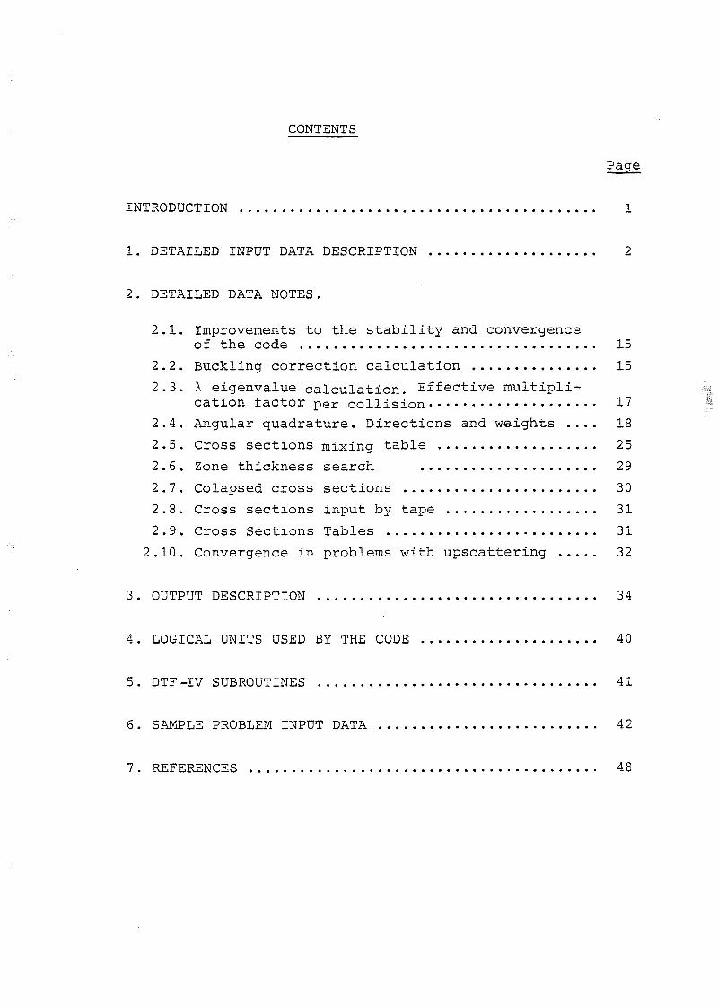
CONTENTS

INTRODÜCTION 1

1. DETAILED INPUT DATA DESCRIPTION 2

2. DETAILED DATA NOTES.

2.1. Improvements to the stability and convergenceof the code 15

2.2. Buckling correction calculation 15

2.3. X eigenvalue calculation. Effective multipli-cation factor per colusión 17

2.4. Angular quadrature. Directions and weights .... 18

2.5. Cross sections mixing table 25

2.6. Zone thickness search 29

2.7. Colapsed cross sections 30

2.8. Cross sections input by tape 31

2.9. Cross Sections Tables 31

2.10. Convergence in problems with upscattering 32

3. OUTPUT DESCRIPTION 34

4 . LOGICAL UNITS USED BY THE CODE 40

5 . DTF -IV SUBROÜTINES 41

6. SAMPLE PROBLEM INPUT DATA 42

7 . REFERENCES 48

- 1 -

INTRODUCTION.

The codes DTF and DTF-II from Los Alamos Laboratory,

solve by the discrete ordinates method the multigroup form of

the neutrón transport equation in one-dimensional plañe, cylin-

drical and spherical geometries• The DTF-IV code is a comple-

te revisión of the DTF code.

DTF-IV is able to perform calculations of independent

source, effective multiplication factor by fission, time absorp-

tion and criticality searches on material concentrations, zone

widths and total dimensión of the system. In the JEN versión

(TRACA) two new eigenvalué calculations have been added, the

effective multiplication factor per colusión and the criticality

search on the buckling valué.

The possibility to input density factors by interval and

bucklings by zone and group has been added; the new versión is

also able to calcúlate and write on tape the sets of colapsed

cross sections weighted with the calculated fluxes, in the

structure of zones and groups asked by the user.

In the process of inner iteration a modification has been

made, in order to get to convergence the problems with negative

self-scatter cross sections, by making a damping in the scalar

flux.

The original DTF-IV code was adapted to the JEN computer

in 1970. Since then, the code has being extensively used for

very different applications and input data. The writting of a

user's manual is justified by the facts that the original report

is not sufficiently explicit on the input data description and

some difficulties can arise on its use, specially for people not

familiar with the transport codes of Los Alamos Laboratory,

together with the necessity of explaining the modifications in-

troduced in the TRACA versión and the experience of its use in

almost all of the possibilities of the code.

- 2 -

This manual will include a detailed input data description,

based on the knowledge and use of this and other codes origi-

nating in Los Alamos.

Some notes explaining the meaning and use of specific

data are given in chapter 2, suggesting giving valúes of them

depending on the problem to solve.

The output description is in chapter 3, giving the quanti-

ties written by the code through all the printed output. The

logical units used by the code and their functions are discussed

in chapter 5, and in the chapter 6 are the sheets with the input

data to be punch on cards for a sample problem. The references

made on the text are in chapter 7.

1. DETAILED INPUT DATA DESCRIPTION.

The input data are divided into the following categories

depending on the formats:

a. A title card (72A1).

b. Input control integers' (1216) on cards 2, 3 and 4.

c. Input control floating point numbers (E12.5) on cards 5,

6 and 7.

d. Problem dependent data on the following cards, in them the

format depends on the subroutine which reads the different

data.

Data Type

Integers

Floating point

Floating point

Subroutine

REA I

REAG

RECS

Format

6(11, 12,

6(11, 12,

6E12.5

19)

E9.4

The first integer II in the REAI and REAG formats indica-

tes the following read options:

- 3 -

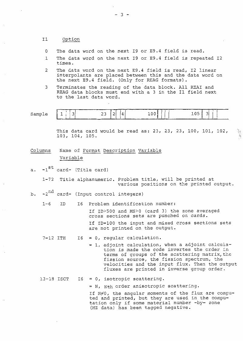
II Option

0 The data word on the next 19 or E9.4 field is read.

1 The data word on the next 19 or E9.4 field is repeated 12times.

2 The data word on the next E9.4 field is read, 12 linearinterpolants are placed between this and the data word onthe next E9.4 field. (Only for REAG formats).

3 Terminates the reading of the data block. All REAI andREAG data blocks must end with a 3 in the II field nextto the last data word.

Sample 23 100 105 !

This data card would be read as: 23, 23, 23, 100, 101, 102,103, 104, 105.

Columns Ñame of Format Description Variable

Variable

- l S t card- (Title card)

1-72

,nd

1-6

Titie alphanumeric. Problem title, will be printed atvarious positions on the printed output

card- (Input control integers)

ID

7-12 ITH

13-18 ISCT

16 Problem Identification number:

If ID>500 and MS>0 (card 3) the zone averagedcross sections sets are punched on cards.

If ID=100 the input and mixed cross sections setsare not printed on the output.

16 = 0 , regular calculation.

= 1, adjoint calculation, when a adjoint calcula-tion is made the code invertes the order interms of groups of the scattering matrix, thefission source, the fission spectrum, thevelocities and the input flux. Then the outputfluxes are printed in inverse group order.

16 = 0 , isotropic scattering.

= N, Mth order anisotropic scattering.

If NrO, the angular moments of the flux are compu-ted and printed, but they are used in the compu-tation only if some material number -by- zone(MZ data) has been tagged negative.

- 4 -

19-24 ISN 16

25-30 IGE 16

31-36 IBL 16

Order of discrete ordinates approximation.

ISN must be even.

For an anisotropic problem should beISN-2.ISCT, and at least 1SN=4.

Geometry

= 1, plañe.= 2, cylindrical.= 3, spherical.

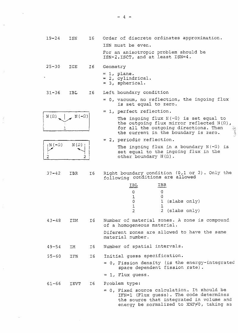
Left boundary condition

= 0, vacuum, no reflection, the ingoing fluxis set equal to zero.

= 1, perfect reflection.

The ingoing flux N(-Í2) is set equal tothe outgoing flux mirror reflected N(fi)for all the outgoing directions. Thenthe current in the boundary is zero.

= 2, periodic reflection.

The ingoing flux in a boundary N(-Q) isset equal to the ingoing flux in theother boundary N(£2) .

37-42 IBR 16

43-48

49-54

55-60

IZM

IM

IFN

16

16

16

61-66 IEVT 16

Right boundary condition (0,1 or 2). Only thefollowing conditions are allowed

IBL IBR

01012

00112

(slabs

(slabs

only)

only)

Number of material zones. A zone is compoundof a homogeneous material.

Diferent zones are allowed to have the samematerial number.

Number of spatial intervals.

Initial guess specification.

= 0, Fission density (is the energy-integratedspace dependent fission rate).

= 1, Flux guess.

Problem type:

= 0, Fixed source calculation. It should beIFN=1 (Flux guess). The code determinesthe source that integrated in volume andenergy be normalized to XNFrO, taking as

_ 5 -

starting point the distributed initialsource (IQM=1); also determines the fluxdistributions.

= 1, keff calculation, effective multiplica-tion factor by fission.

= 2, Time absorption calculation, determines .a in the eat time dependent flux assump-tion.

= 3, Concentration search (c), of a materialor nuclide to achieve criticality or theparametric eigenvalue if IPVTÔ. Specialmixtures instructions (MB, MC, XMD) mustbe entered in the problem dependent datasection.

= 4, Zone width search (6), of a zone or zo-nes to achieve criticality or the para-metric eigenvalue if IPVTrO. Radial mo-difiers (RM) must be entered in the pro-blem dependent data section.

= 5 , System total dimensión search (a), uni-form variation of all system dimensionsto achieve criticality or the parametriceigenvalue if IPVTÔ.

= 6, Buckling search to achieve criticalityor the parametric eigenvalue if IPVTÔ.Then, BF, DY and DZ must be entered.

=-1, X eigenvalue calculation, effective mul-tiplication factor per colusión (SeeNote 2.3).

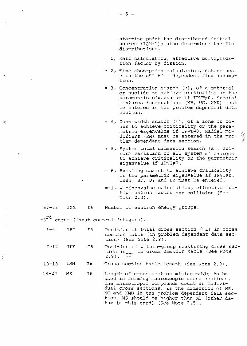
67-72 IGM 16 Number of neutrón energy groups.

-3 card- (input control integers).

1-6 IHT 16 Position of total cross section (afc) in crosssection table (in problem dependent data sec-tion) (See Note 2.9).

7-12 IHS 16 Position of within-group scattering cross sec-tion (a ) in cross section table (See Note2.9). g g

13-18 IHM 16 Cross section table length (See Note 2.9).

19-24 MS 16 Length of cross section mixing table to beused in forming macroscopic cross sections.The anisotropic compounds count as indivi-dual cross sections. Is the dimensión of MB,MC and XMD in the problem dependent data sec-tion. MS should be higher than MT (other da-tum in this card) (See Note 2.5).

- 6 -

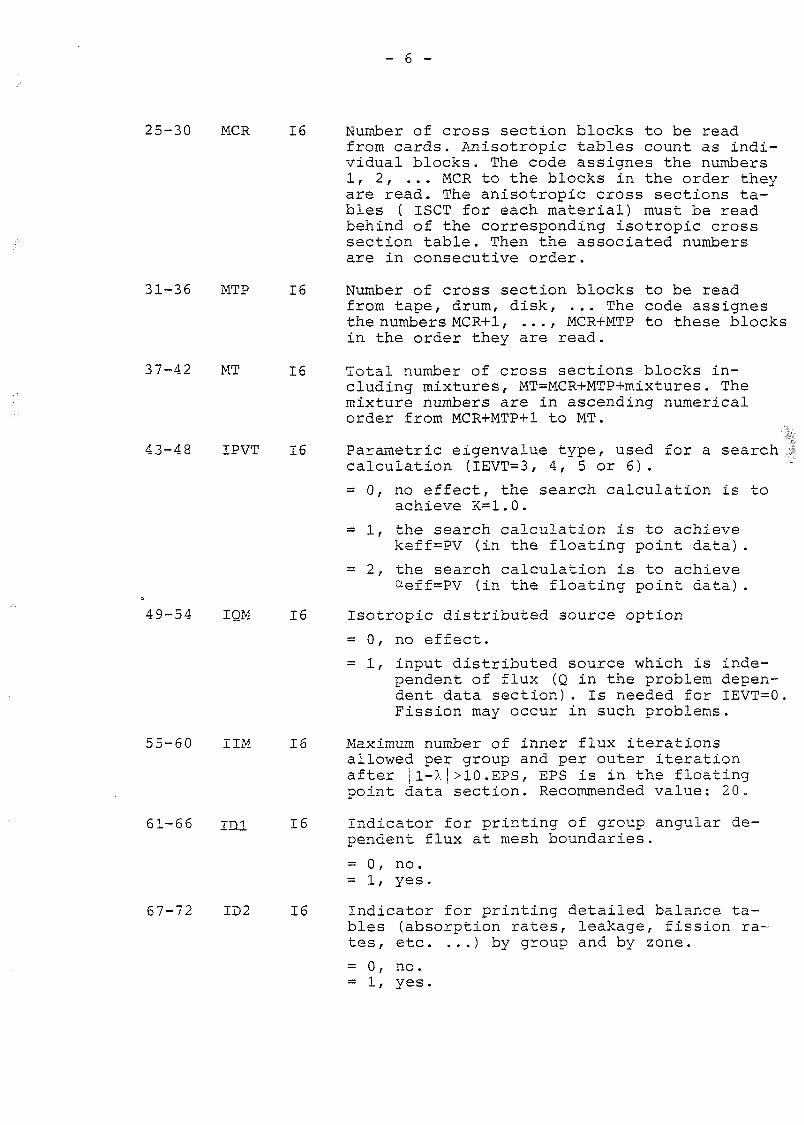
25-30 MCR 16 Number of cross section blocks to be readfrom cards. Anisotropic tables count as indi-vidual blocks. The code assignes the numbers1, 2, ... MCR to the blocks in the order theyare read. The anisotropic cross sections ta-bles ( ISCT for each material) must be readbehind of the corresponding isotropic crosssection table. Then the associated numbersare in consecutive order.

31-36 MTP 16 Number of cross section blocks to be readfrom tape, drum, disk, ... The code assignesthe numbers MCR+1, ..., MCR+MTP to these blocksin the order they are read.

37-42 MT 16 Total number of cross sections blocks in-cluding mixtures, MT=MCR+MTP+mixtures. Themixture numbers are in ascending numericalorder from MCR+MTP+1 to MT.

43-48 IPVT 16 Parametric eigenvalue type, used for a searchcalculation (IEVT=3, 4, 5 or 6).

= 0, no effect, the search calculation is toachieve K=1.0.

= 1, the search calculation is to achievekeff=PV (in the floating point data).

= 2, the search calculation is to achieveaeff=PV (in the floating point data).

49-54 IQM 16 Isotropic distributed source option

= 0, no effect.

= 1, input distributed source which is inde-pendent of flux (Q in the problem depen-dent data section). Is needed for IEVT=0.Fission may occur in such problems.

55-60 1IM 16 Máximum number of inner flux iterationsallowed per group and per outer iterationafter |1-X|>10.EPS, EPS is in the floatingpoint data section. Recommended valué: 20.

61-66 i m 16 Indicator for printing of group angular de-pendent flux at mesh boundaries.

= 0, no.= 1, yes.

67-72 ID2 16 Indicator for printing detailed balance ta-bles (absorption rates, leakage, fission ra-tes, etc. ...) by group and by zone.

= 0, no .= 1, yes.

_ 7 —

-4 card- (input control integers).

1-6 ID3

7-12 ID4

13-18 ICM

19-24 NFF

25-30 IC

31-36 IIL

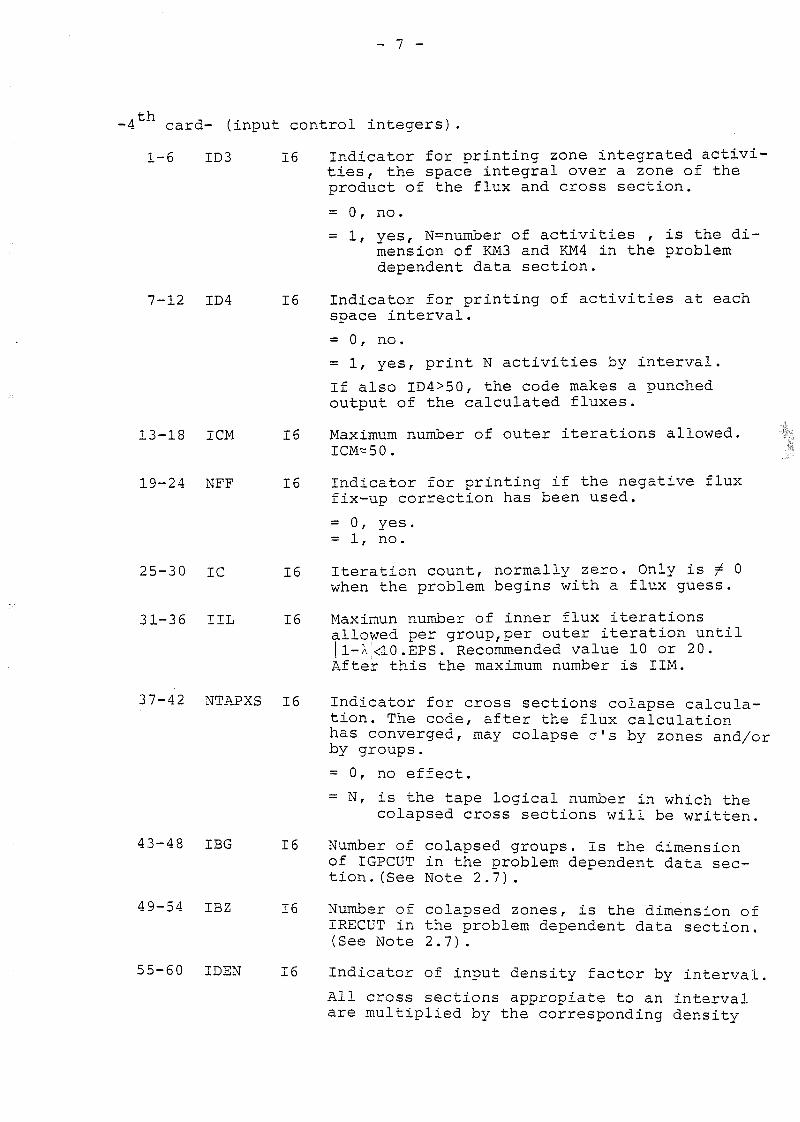
16 Indicator for printing zone integrated activi-ties, the space integral over a zone of theproduct of the flux and cross section.

= 0, no .

= 1, yes, N=number of activities , is the di-mensión of KM3 and KM4 in the problemdependent data section.

16 Indicator for printing of activities at eachspace interval.

= 0, no.

= 1, yes, print N activities by interval.

If also ID4>50, the code makes a punchedoutput of the calculated fluxes.

16 Máximum number of outer iterations allowed.

16

16

16

Indicator for printing if the negative fluxfix-up correction has been used.

= 0, yes.= 1, no.

Iteration count, normally zero. Only is f 0when the problem begins with a flux guess.

Maximun number of inner flux iterationsallowed per group,per outer iteration until[ 1-A'<10 .EPS. Recommended valué 10 or 20.After this the máximum number is IIM.

37-42 NTAPXS 16

43-48 IBG 16

49-54 IBZ 16

Indicator for cross sections colapse calcula-tion. The code, after the flux calculationhas converged, may colapse a's by zones and/orby groups.

= 0, no effect.

= N, is the tape logical number in which thecolapsed cross sections will be written.

Number of colapsed groups. Is the dimensiónof IGPCUT in the problem dependent data sec-tion. (See Note 2.7).

Number of colapsed zones, is the dimensión ofIRECÜT in the problem dependent data section.(See Note 2.7) .

55-60 IDEN 16 Indicator of input density factor by interval

All cross sections appropiate to an intervalare multiplied by the corresponding density

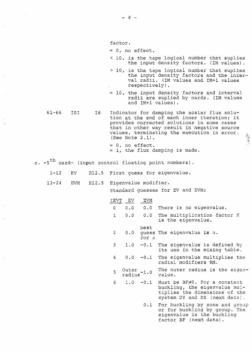
factor.

= 0, no effect.

< 10, is the tape logical number that supliesthe input density factors. (IM valúes).

> 10, is the tape logical number that supliesthe input density factors and the inter-val radii. (IM valúes and IM+1 valúesrespectively).

= 1 0 , the input density factors and intervalradii are suplied by cards. (IM valúesand IM+1 valúes).

61-66 ISI 16 Indicator for damping the scalar flux solu-tion at the end of each inner iteration; itprovides corrected solutions in some casesthat in other way result in negative sourcevalúes, terminating the execution in error.(See Note 2.1).

= 0, no effect.= 1, the flux damping is made.

c. -5 card- (input control floating point numbers).

1-12 EV E12.5 First guess for eigenvalue.

13-24 EVM E12.5 Eigenvalue modifier.

Standard guesses for EV and EVM:

IEVT EV EVM

0 0.0 0.0 There is no eigenvalue.

1 0.0 0.0 The multiplication factor Kis the eigenvalue.

best2 0.0 guess The eigenvalue is a.

for a

3 1.0 -0.1 The eigenvalue is defined byits use in the mixing table.

4 0.0 -0.1 The eigenvalue multiplies theradial modifiers RM.

Outer 1 0 The outer radius is the eigen-radius " valué.

6 1.0 -0.1 Must be BFÔ. For a constantbuckling, the eigenvalue mul-tiplies the dimensions of thesystem DY and DZ (next data),

0.1 For buckling by zone and groupor for buckling by group. Theeigenvalue is the bucklingfactor BF (next data) .

- 9 -

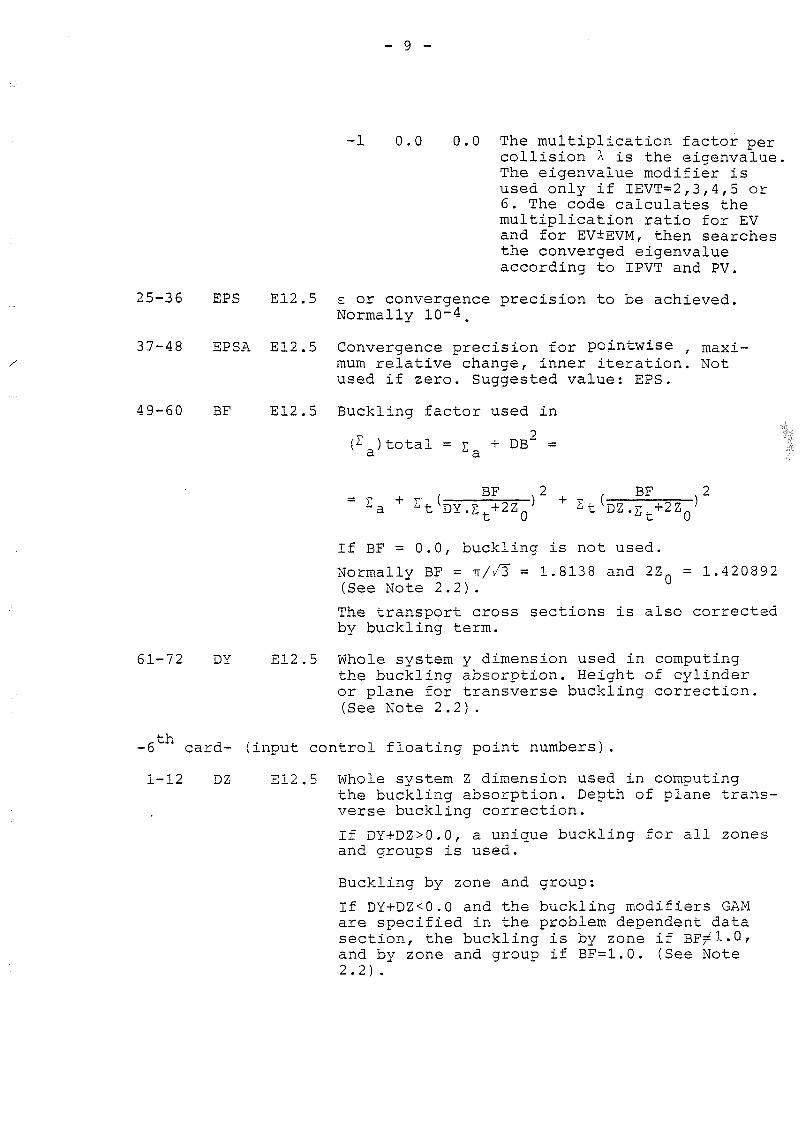
-1 0.0 0.0 The multiplication factor percolusión X is the eigenvalue.The eigenvalue modifier isused only if IEVT=2,3,4,5 or6. The code calculates themultiplication ratio for EVand for EViEVM, then searchesthe converged eigenvalueaccording to IPVT and PV.

25-36 EPS E12.5 e or convergence precisión to be achieved.Normally 10-4.

37-48 EPSA E12.5 Convergence precisión for pointwise , maxi-./ mum relative change, inner iteration. Not

used if zero. Suggested valué: EPS.

49-60 BF E12.5 Buckling factor used in

(£ ) total = v + DB2 =a a

, B F 2 , B F 2S r t ^ D Y S + 2 Z } + Z t ^ D Z + 2 Z }

If BF = 0.0, buckling is not used.

Normally BF = TT//3~ = 1.8138 and 2Z = 1.420892(See Note 2.2).

The transport cross sections is also correctedby buckling term.

61-72 DY E12.5 Whole system y dimensión used in computingthe buckling absorption. Height of cylinderor plañe for transverse buckling correction.(See Note 2.2) .

-6 card- (input control floating point numbers).

1-12 DZ E12.5 Whole system Z dimensión used in computingthe buckling absorption. Depth of plañe trans-verse buckling correction.

If DY+DZ>0.0, a unique buckling for all zonesand groups is used.

Buckling by zone and group:

If DY+DZ<0.0 and the buckling modifiers GAMare specified in the problem dependent datasection, the buckling is by zone if BFr 1 • 0 rand by zone and group if BF=1.0. (See Note2.2) .

- 10 -

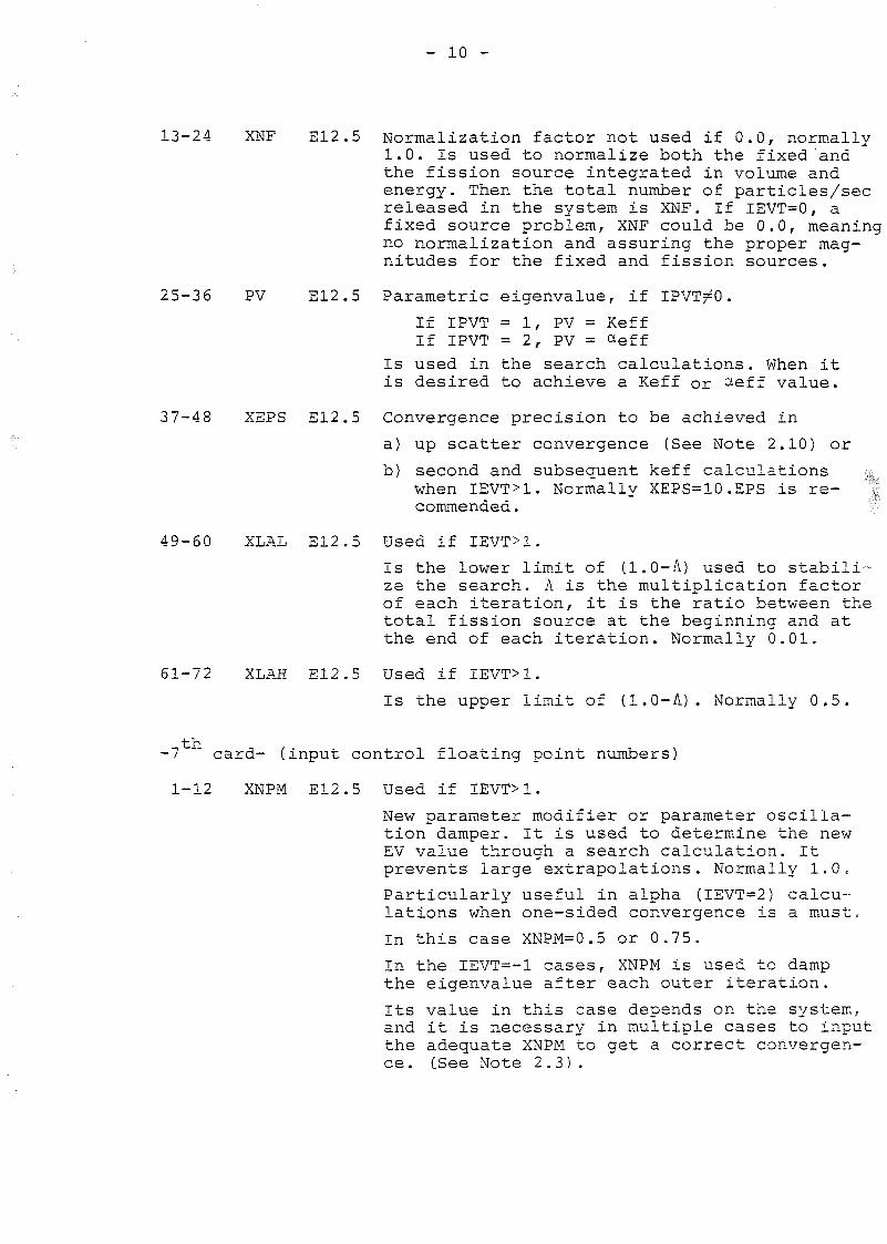
13-24 XNF E12.5 Normalization factor not used if 0.0, normally1.0. Is used to normalize both the fixed andthe fission source integrated in volume andenergy. Then the total number of particles/secreleased in the system is XNF. If IEVT=0, afixed source problem, XNF could be 0.0, meaningno normalization and assuring the proper mag-nitudes for the fixed and fission sources.

25-36 PV E12.5 Parametric eigenvalue, if IPVTÔ.

If IPVT = 1, PV = KeffIf IPVT = 2, PV = <*eff

Is used in the search calculations. When itis desired to achieve a Keff or cteff valué.

37-48 XEPS E12.5 Convergence precisión to be achieved in

a) up scatter convergence (See Note 2.10) or

b) second and subsequent keff calculationswhen IEVT>1. Normally XEPS=10.EPS is re-commended.

49-60 XLAL E12.5 üsed if IEVT>1.

Is the lower limit of (1.0-A) used to stabili-ze the search. A is the multiplication factorof each iteration, it is the ratio between thetotal fission source at the beginning and atthe end of each iteration. Normally 0.01.

61-72 XLAH E12.5 Used if IEVT>1.

Is the upper limit of (1.0-A). Normally 0.5.

-7 card- (input control floating point numbers)

1-12 XNPM E12.5 Used if IEVT>1.

New parameter modifier or parameter oscilla-tion damper. It is used to determine the newEV valué through a search calculation. Itprevents large extrapolations. Normally 1.0.

Particularly useful in alpha (IEVT=2) calcu-lations when one-sided convergence is a must.

In this case XNPM=0.5 or 0.75.

In the IEVT=-1 cases, XNPM is used to dampthe eigenvalue after each outer iteration.

Its valué in this case depends on the system.and it is necessary in múltiple cases to inputthe adequate XNPM to get a correct convergen-ce. (See Note 2.3).

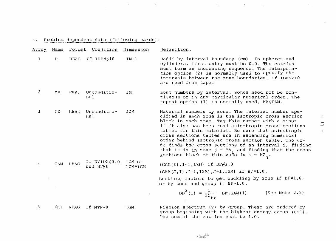
4. Problem dependent data (following cards).

Array Mame Forma t Condition Dimensión

1 R REAG If IDENÎO IM+1

MA REAI Unconditio- IMnal

MZ REAI Unconditio- IZMnal

GAM REAGIf DY-I-DZ O.O IZM orand BFÔ IZM*IGM

XKI REAG If MTP=0 IGM

Definition.

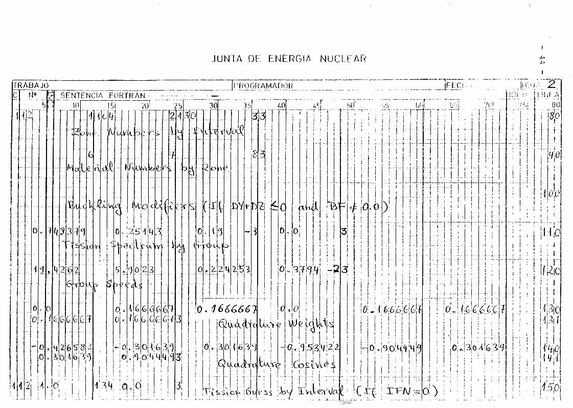
Radii by interval boundary (cm). In spheres andoylinders, first entry must be 0.0. The entriesmust form an increasing sequence. The interpola-tion option (2) is normally used to specify theintervals between the zone boundaries. If IDEN>xOare read from tape.

Zone numbers by interval. Zones need not be con-tiguous or in any particular numerical order. Therepeat option (1) is normally used. MAÎZM.

Material numbers by zone. The material number spe-cified in each zone is the isotropic cross sectionblock in each zone. Tag this number with a minusif it also has been read anisotropic cross sectionstables for this material. Be sure that anisotropiccross sections tables are in ascending numericalorder behind isotropic cross section table. The co-de finds the cross sections of an interval i, findingthat it is in zone j = MA. and finding that the crosssections block of this zone is k = MZ..

(GAM(I),1=1,IZM) if BF^l.O

(GAM(J,I),1=1,IZM),J=1,IGM) if BF-1.0.

Buckling factors to get buckling by zone if BF^l.O,or by zone and group if BF=1.0.

2._. 13E BF.GAM(I) (See Note 2.2)

tr

Fission spectrum (x) by group. These are ordered bygroup beginning with the highest energy group (g=l),The sum of the entries must be 1.0.

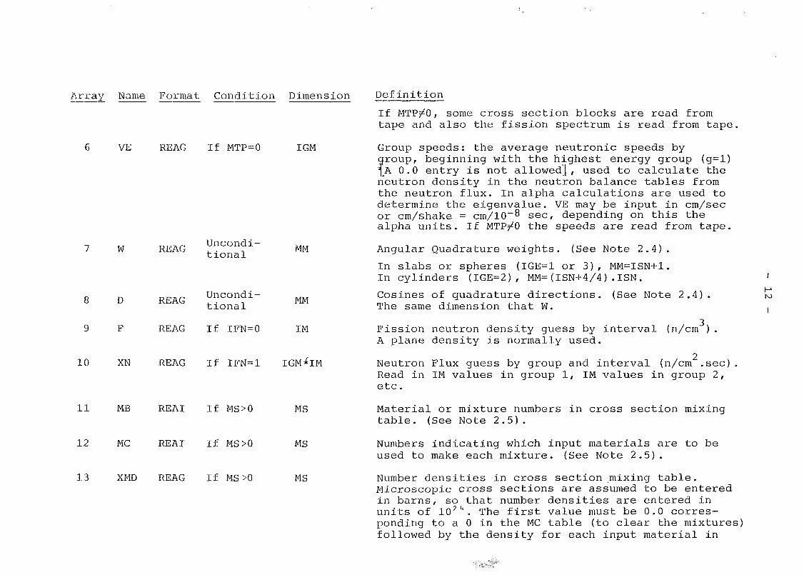
Array Ñame Format Condition Dimensión

VE REAG If MTP=0

W

8 D

REAG

REAG

Uncondi-tional

11 MB REAI If MS>0

12 MC REAI If MS>0

13 XMD REAG If MS>0

IGM

MM

MMtional

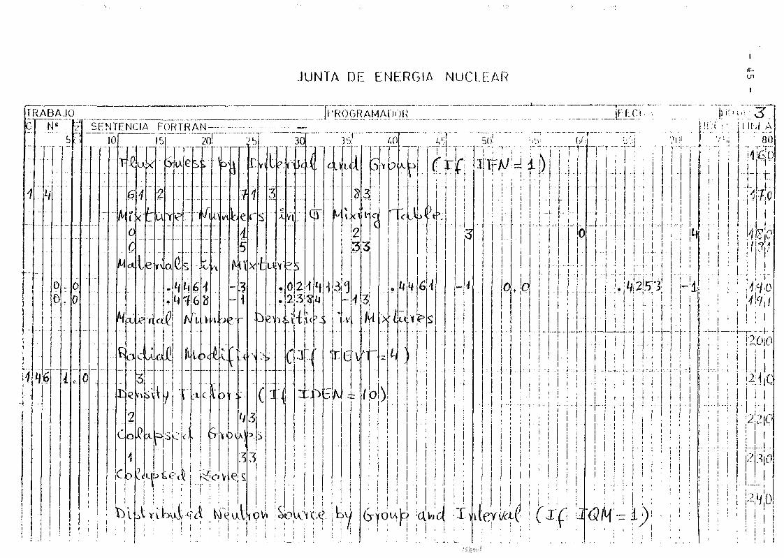
9 F REAG If IFN=0 IM

10 XN REAG If IFN=1 IGMÎM

MS

MS

MS

Definition

If MTPÔ, some cross section blocks are read fromtape and also the fission spectrum is read from tape.

Group speeds: the average neutronic speeds by

?roup, beginning with the highest energy group (g=l)A 0.0 entry is not allowedj, used to calcúlate theneutrón density in the neutrón balance tables fromthe neutrón flux. In alpha calculations are used todetermine the eigenvalue. VE may be input in cm/secor cm/shake = cm/10~8 sec, depending on this thealpha units. If MTPÔ the speeds are read from tape.

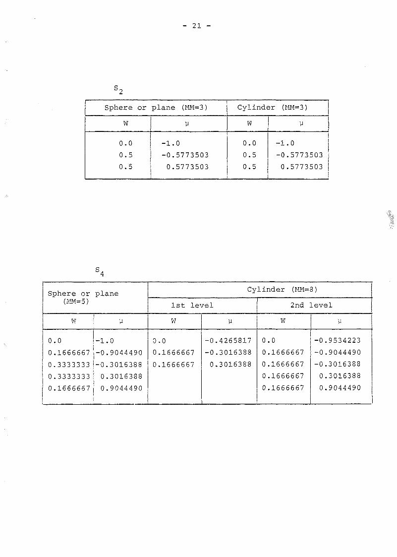
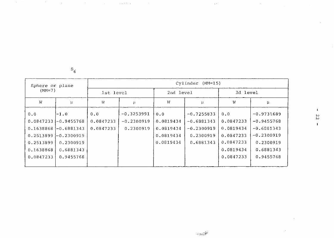
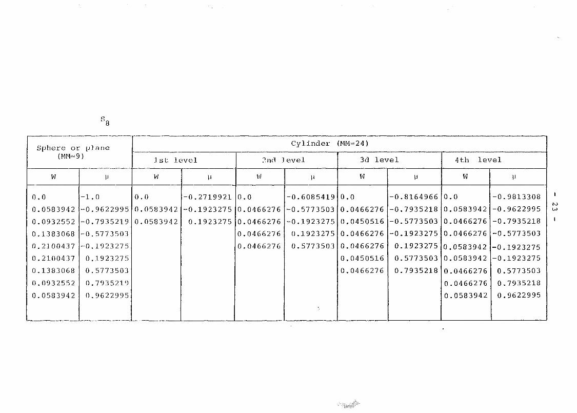
Angular Quadrature weights. (See Note 2.4).

In slabs or spheres (IGE=1 or 3), MM=ISN+1.In cylinders (IGE=2), MM=(ISN+4/4).ISN.

Cosines of quadrature directions. (See Note 2.4).The same dimensión that W.

3Fission neutrón density guess by interval (n/cm ).A plañe density is normally used.

2Neutrón Flux guess by group and interval (n/cm .sec).Read in IM valúes in group 1, IM valúes in group 2,etc.

Material or mixture numbers in cross section mixingtable. (See Note 2.5).

Numbers indicating which input materials are to beused to make each mixture. (See Note 2.5).

Number densities in cross section mixing table.Microscopic cross sections are assumed to be enteredin barns, so that number densities are entered inunits of 102'1. The first valué must be 0.0 corres-ponding to a 0 in the MC table (to clear the mixtures)followed by the density for each input material in

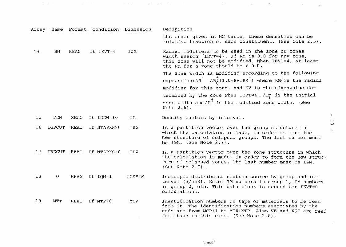
Array Ñame Format Condition Dimensión

14. RM REAG If IEVT=4 IZM

15 DEN REAG If IDEN=10 IM

16 IGPCUT REAI If NTAPXS>0 IBG

17 IRECUT REAI If NTAPXS>0 IBZ

18 Q REAG If IQM=1 IGM*IM

19 MTT REAI If MTP>0 MTP

Definition

the order given in MC table, these densities can berelative fraction of each constituent. (See Note 2.5).

Radial modifiers to be used in the zone or zoneswidth search (IEVT=4). If RM is 0.0 for any zone,this zone will not be modified. When IEVT=4, at leastthe RM for a zone should be ^ 0.0.

The zone width is modified eccording to the following

expressioniAR"1 =AR^ (1. 0+EV.RM"5) where RM^ is the radial

modifier for this zone. And EV is the eigenvalue de-

termined by the code when IEVT=4 , AR~ is the initial

zone width and AR is the modified zone width. (SeeNote 2.6).

Density factors by interval.

Is a partition vector over the group structure inwhich the calculation is made, in order to form thenew structure of colapsed groups. The last number mustbe IGM. (See Note 2.7).

Is a partition vector over the zone structure in whichthe calculation is made, in order to form the new struc-ture of colapsed zones. The last number must be IZM.(See Note 2.7) .

Isotropic distributed neutrón source by group and in-terval (n/cm3). Enter IM numbers in group 1, IM numbersin group 2, etc. This data block is needed for IEVT=0calculations.

Identification numbers on tape of materials to be readfrom it. The identification numbers associated by thecode are from MCR+1 to MCR+MTP. Also VE and XKI are readfrom tape in this case. (See Note 2.8).

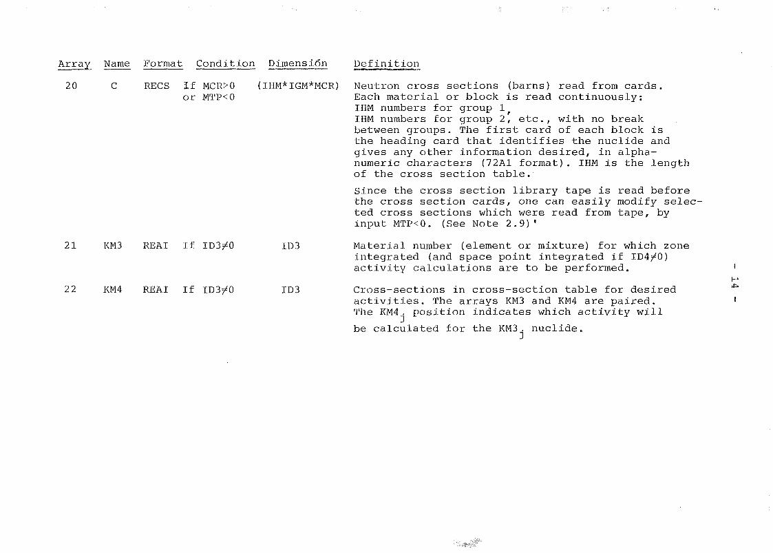
Array Narne Format Condition Dimensión Def inition

20 RECS If MCR>0or MTP<0

(IHM*IGM*MCR)

21

22

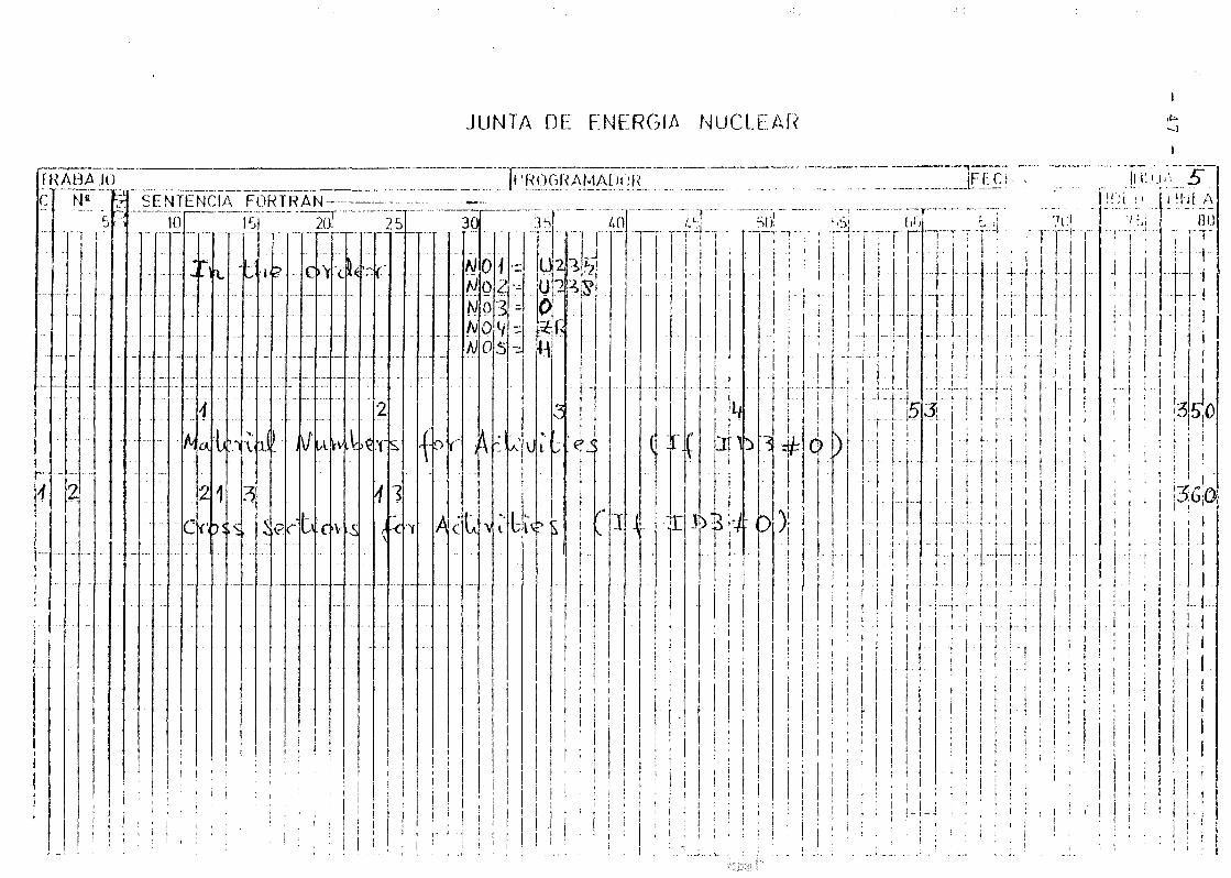
KM3

KM4

REAI If

REAI If

ID3

ID3

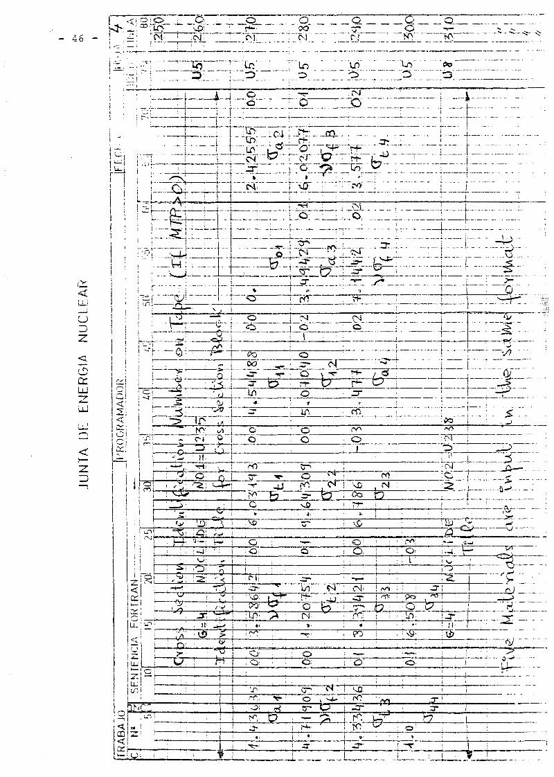
Neutrón cross sections (barns) read from cards.Each material or block is read continuously:IHM numbers for group lfIIIM numbers for group 2, etc., with no breakbetween groups. The first card of each block isthe heading card that identifies the nuclide andgives any other information desired, in alpha-numeric characters (72A1 format). IHM is the lengthof the cross section table.

Since the cross section library tape is read beforethe cross section cards, one can easily modify selec-ted cross sections which were read from tape, byinput MTP<0. (See Note 2.9)'

Material number (element or mixture) for which zoneintegrated (and space point integrated if 104^0)activity calculations are to be performed.

Cross-sections in cross-section table for desiredactivities. The arrays KM3 and KM4 are paired.The KM4. position indicates which activity will

be calculated for the KM3. nuclide.

- 15 -

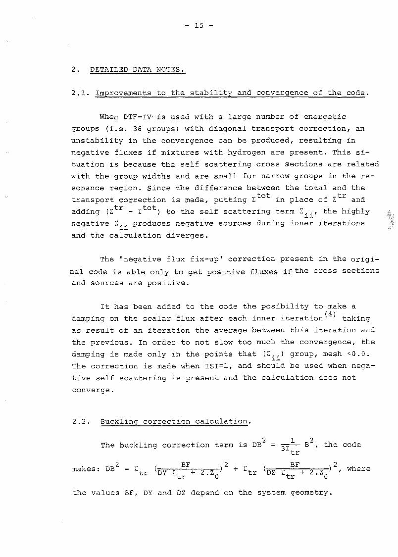
2. DETAILED DATA NOTES.

2.1. Improvements to the stability and convergence of the code.

When DTF-IV- is used with a large number of energetic

groups (i.e. 36 groups) with diagonal transport correction, an

unstability in the convergence can be produced, resulting in

negative fluxes if mixtures with hydrogen are present. This si-

tuation is because the self scattering cross sections are related

with the group widths and are small for narrow groups in the re-

sonance región. Since the difference between the total and the

transport correction is made, putting Z in place of I and

adding (E r - E ) to the self scattering term I.., the highly

negative E., produces negative sources during inner iterations

and the calculation diverges.

The "negative flux fix-up" correction present in the origi-

nal code is able only to get positive fluxes if the cross sections

and sources are positive.

It has been added to the code the posibility to make a(4)

damping on the scalar flux after each inner iteration taking

as result of an iteration the average between this iteration and

the previous. In order to not slow too much the convergence, the

damping is made only in the points that (2..) group, mesh <0.0.

The correction is made when ISI=1, and should be used when nega-

tive self scattering is present and the calculation does not

converge.

2.2. Buckling correction calculation.

2 1 2The buckling correction term is DB = •=-=— B , the code

¿tr2 "Rf? 0 VK1P *?

m a k e s : D B = E f c r í p Y ^ + 2 . Z Q] + Z t r ( D Z E f c r + 2 . Z Q

] ' w h e r e

the valúes BF, DY and DZ depend on the system geometry.

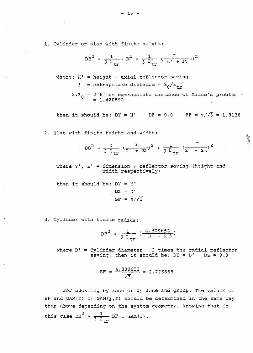
- 16 -

1. Cylinder or slab with finite height:

B -

where: H1 = height + axial reflector saving

i = extrapólate distance = zn/^tr

2.Zn = 2 times extrapólate distance of Milne's problem -U = 1.420892

then it should be: DY = H1 DZ = 0.0 BF = TT//3 = 1.8138

2. Slab with finite height and width:

rm ( ) + ( )D " 3 !• ^ Y 1 + 25. 3 E

+ z ' + 2 ¿ ;

"Cx* • x r

where Y', Z1 = dimensión + reflector saving (height andwidth respectively)

then it should be: DY = Y1

DZ = Z1

BF = TT/ZI

3. Cylinder with finite radius:

_ 2 1 , ¿1.809652ua ~ 3 i+

v D1 + 2 5,

where D1 = Cylinder diameter + 2 times the radial reflectorsaving, then it should be: DY = D1 DZ = 0.0

BP - 4.809652 _ 77(-occ

For buckling by zone or by zone and group. The valúes of

BF and GAM(I) or GAM(j,I) should be determined in the same way

than above depending on the system geometry, knowing that in

this case DB2 = -s-J— BF . GAMtl) .

- 17 -

2.3. X eigenvalue calculation. Effective multiplication factor

per colusión.

Calculation of X eigenvalue has being incorporated to the

original code. It divides the number of secondary neutrons per

colusión, this is, the number of neutrons per scattering and

fission, while k eigenvalue divides only the neutrons per

fission.

The integrodifferential Boltzmann equation of the virtual(18)critical reactor with A is

(L+Rt)ó;v + | (S+F)<J>X = 0

where, L = -Q.V., is the linear differential operator of leakage

R = -Z (r,v,t)., is the multiplicativa operator of extrac-tion.

S = | dv'dr'Z (r,v^Ó'-^v,fi,t) . , is the linear integralj s operator of scattering.

F = i/4-iT.Xp jdv'dQ'vív1 ) 2 - (r,v' ,t) ., is the linear inte-p j

gral operator of prompt and delayed fissions.

Integrating over the whole phase space RxV x r results:

<(S-rF)>Ó.A 0

0 <(L-rR )>(5,t A Q

is the ratio between neutrons produced by collisions in the unit

of time in the reactor, corresponding to the virtual flux, and the

losses of neutrons in t h e u n i t o f time due to leakage through

the free surface of the reactor and to collisions in the reactor,

corresponding also to the virtual flux.

This eigenvalue is calculated by the code if: IZVT=-1.

For some systems, principally for the thermal ones (with

upscattering) the calculation of the converged solution in X,

- 18 -

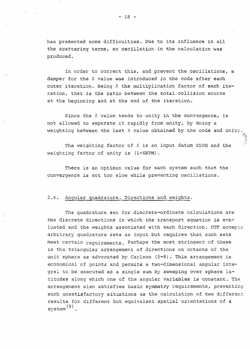
has presented some difficulties. Due to its influence in all .

the scattering terms, an oscillation in the calculation was

produced.

In order to correct this, and prevent the oscillations, a

damper for the A valué wa-s introduced in the code after each

outer iteration. Being A the multiplication factor of each ite-

ration, that is the ratio between the total colusión source

at the beginning and at the end of the iteration.

Since the A valué tends to unity in the convergence, is

not allowed to sepárate it rapidly from unity, by doing a

weighting between the last A valué obtained by the code and unity

The weighting factor of A is an input datum XNPM and the

weighting factor of unity is (1-XNPM).

There is an optimun valué for each system such that the

convergence is not too slow while preventing oscillations.

2.4. Angular quadrature. Directions and weights.

The quadrature set for discrete-ordinate calculations are

the discrete directions in which the transport equation is eva-

luated and the weights associated with each direction. DTF accepts

arbitrary quadrature sets as input but requires that such sets

meet certain reauirements. Perhaps the most stringent of these

is the triangular arrangement of directions on octants of the

unit sphere as advocated by Carlson (5-8). This arrangement is

economical of points and permits a two-dimensional angular inte-

gral to be executed as a single sum by sweeping over sphere la-

titudes along which one of the angular variables is constant. The

arrangement also satisfies basic symmetry requirements, preventing

such unsatisfactory situations as the calcuiation of two different

results for different but equivalent spatial orientations of a(9)

system

- 19 -

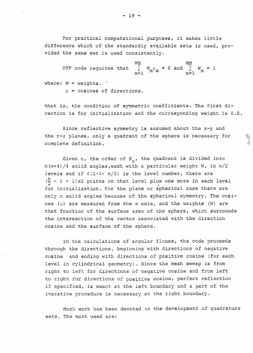
For practical computational purposes, it makes little

difference which of the standardly available sets is used, pro-

vided the same set is used consistently.

MM MMDTF code requires that 1 W u = 0 and J W = 1

m=l m=l

where: W = wéights. '

y = cosines of directions.

that is, the condition of symmetric coefficients. The first di-

rection is for initialization and the corresponding weight is 0.0.

Since reflective symmetry is assumed about the x-y and

the r-z planes, only a quadrant of the sphere is necessary for

complete definition.

Given n, the order of S , the quadrant is divided into

n(n+4)/4 solid angles,each with a particular weight W, in n/2

levéis and if £(1<£< n/2) is the level number, there are

(~ - t + I)x2 points on that level plus one more in each level

for initialization. For the plañe or spherical case there are

only n solid angles because of the spherical symmetry. The cosi-

nes (y) are measured from the x axis, and the weights (W) are

that fraction of the surface área of the sphere, which surrounds

the intersection of the vector associated with the direction

cosine and the surface of the sphere.

In the calculations of angular fluxes, the code proceeds

through the directions, beginning with directions of negative

cosine and ending with directions of positive cosine (for each

level in cylindrical geometry). Since the mesh sweep is from

right to left for directions of negative cosine and from left

to right for directions of positive cosine, perfect reflection

if specified, is exact at the left boundary and a part of the

iterative procedure is necessary at the right boundary.

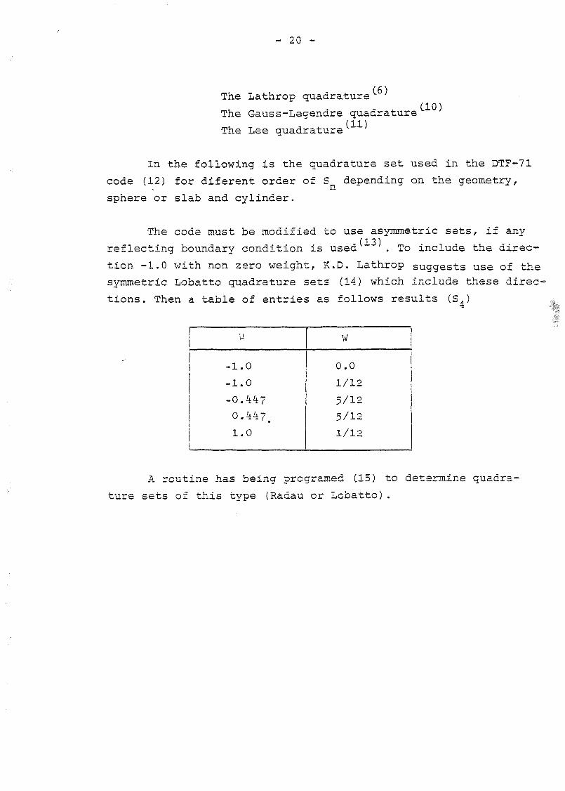
Much work has been devoted to the development of quadrature

sets. The most used are:

- 20 -

The Lathrop quadrature (6)

The Gauss-Legendre quadrature

The Lee auadrature

CIO)

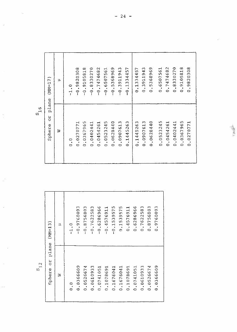
In the following is the quadrature set used in the DTF-71

12) for diferent order

sphere or slab and cylinder.

code (12) for diferent order of S depending on the geometry,

The code must be modified to use asymmetric sets, if any

reflecting boundary condition is used . To include the direc-

tion -1.0 with non zero weight, K.D. Lathrop suggests use of the

symmetric Lobatto quadrature sets (14) which include these direc-

tions. Then a table of entries as follows results <s4>

u

-1.0

-1.0

0.4^7.1.0

w

0.0

1/12

5/12

5/12

1/12

A routine has being programed (15) to determine quadra-

ture sets of this type (Radau or Lobatto).

- 21 -

Sphere or plañe (MM=3)

W

0.0

0.5

0.5

y

-1.0

-0.5773503

0.5773503

Cylinder (MM=3)

W

0.0

0.5

0.5

U

-1.0

-0.5773503

0.5773503

Sphere or(MM=5)

W

0.0

0.1666667

0.3333333

0.3333333

0.1666667

plañe

u

-1.0

-0.9044490

-0.3016388

0.3016388

0.9044490

Cylinder (MM=8)

Ist level

W

0.0

0.1666667

0.1666667

y

-0.4265817

-0.3016388

0.3016388

2nd level

W

0.0

0.1666667

0.1666667

0.1666667

0.1666667

y

-0.9534223

-0.9044490

-0.3016388

0.3016388

0.9044490

Sphere or(MM=7)

W

0.0

0.0847233

0.1638868

0.2513899

0.2513899

0.1638868

0.0847233

plañe

y

-1.0

-0.9455768

-0.6881343

-0.2300919

0.2300919

0.6881343

0.9455768

Cylinder (MM=15)

Ist level

W

0.0

0.0847233

0.0847233

.-0.3253991

-0.2300919

0.2300919

2nd level

W

0.0

0.0819434

0.0819434

0.0819434

0.0819434

y

-0.7255833

-0.6881343

-0.2300919

0.2300919

0.6881343

3d level

W

0.0

0.0847233

0.0819434

0.0847233

0.0847233

0.0819434

0.0847233

y

-0.9731689

-0.9455768

-0.6881343

-0.2300919

0.2300919

0.6881343

0.9455768

I

Sphere or(MM=9

W

0.0

0.0583942

0.0932552

0.1383068

0.2100437

0.2100437

0.1383068

0.0932552

0.0583942

plañe)

-1.0

-0.9622995

-0.7935219

-0.5773503

-0.1923275

0.1923275

0.5773503

0.7935219

0.9622995

Cylinder (MM=24)

isL level

W

0.0

0.0583942

0.0583942

U

-0.2719921

-0.1923275

0.1923275

?.nd level

W

0.0

0.0466276

0.0466276

0.0466276

0.0466276

H

-0.6085419

-0.5773503

-0.1923275

0.1923275

0.5773503

3d level

W

0.0

0.0466276

0.0450516

0.0466276

0.0466276

0.0450516

0.0466276

M

-0.8164966

-0.7935218

-0.5773503

-0.1923275

0.1923275

0.5773503

0.7935218

4th level

W

0.0

0.0583942

0.0466276

0.0466276

0.0583942

0.0583942

0.0466276

0.0466276

0.0583942

-0.9813308

-0.9622995

-0.7935218

-0.5773503

-0.1923275-0.1923275

0.5773503

0.7935218

0.9622995

U)

- 24 -

VO

, .

rH112323

0)

(C

¡H0

0)SH0!

Cuco

ES

orH1

oo

coorooCN00

enol

rH

r-or~CNO

O

00

coLDOrH

enoI

IDVO

en[-,VOroO

O

O[»»

CNOrooo00

o1

rH•31

CNO

O

o

CNCO

vo[~~• " *

o1

rHVDCN

unO

o

vounoIDVO

o1

LO^*CN

roCNinoo

en

ocovo00

uno1

o

COCN

vooo

ro"enHrHenrool

oorHVOp-

oenO

o

LD•"=?

3*

oooorH

O1

rovor>j

un•=?

rH

O

t--

m•«a»• < *

rororH

O

rovorsLD

'a*•«a*

rH

O

00

enrHrH

en00

o

00HVO

oenoo

envoencoVDOOin

o

o

COOÍ

vooo

voLD

oLO

voo

in

CN00CNLDO

O

CNCO

voP--"SI1

O

rHVOCN**

un

oo

or-CN

o00

ro00

o

rH

CNO'a*oo

00rHCO

unorHeno

invoeni—vorooo

coooooCNCO

eno

rHp~

ror~CNO

O

CNrH

en

00

1

Creír-íCu

M0

0)ÍH0)r¡Cuce

¡s

orH1

oO

00

enooVD

enoi

enovovovorooo

00

ccoVDinr-.coo1

• = *

r-vovoCNLO

oo

oocoinCNCNVO

r~ci

ro00

enorH

vooo

VO

voenVD

coCN

vooi

rHLDOrH

t—O

O

rHrHenvoLO

O1

rH

envocot-~orH

o

in[--.

unenroLOrH

O1

rH*SPOvo[-

vorH

O

[~

unen00inrH

O

oVD[~

VDrH

O

rHrH

envo[-LO

O

rHenvocor-orH

O

VD

voenvocoCN

voo

rHunorH

r-oo

00

counCNCN

vo

o

00

ooenorHvooo

ooocovounr-~coo

vovoCN

unoo

roenoovop-

cno

enovoVDVD

rooo

- 25 -

A system of codes DOQDP/ADOQ (16-1?) has been recently

received at JEN from the program library, which are used to ge-

nerated direction sets. If a fully synimetric quadrature is desired,

DOQDP can genérate the direction cosines to be used. If other

than a fully symmetric quadrature is to t>e generated, the user

must supply the appropiate direction cosines. Once the directions

are specified, the code will genérate the quadrature weights.

The ADOQ code combines asymmetric quadrature data with symmetric

quadrature data in one hemisphere of the unit S sphere, adjusts

the level weights of the last asymmetric level to match the

symmetric level, and verifies the various relationships these

data must satisfy.

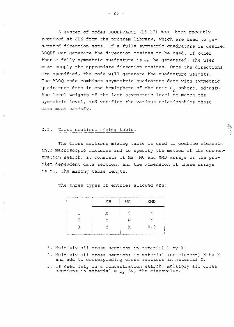
2.5. Cross sections mixing table.

The cross sections mixing table is used to combine elements

into macroscopic mixtures and to specify the method of the concen-

tration search. It consists of MB, MC and XMD arrays of the pro-

blem dependent data section, and the dimensión of these arrays

is MS, the mixing table length.

The three types of entries allowed are:

1

2

3

MB

M

M

M

MC

0

N

M

XMD

X

X

0 . 0

1. Multiply all cross sections in material M by X.

2. Multiply all cross sections in material (or element) N by Xand add to corresponding cross sections in material M.

3. Is used only in a concentration search, multiply all crosssections in material M by EV, the eigenvalue.

- 26 -

In the case of anisotropic cross sections blocks, each •

block should be treated as an independent material or element

in the cross sections mixing table.

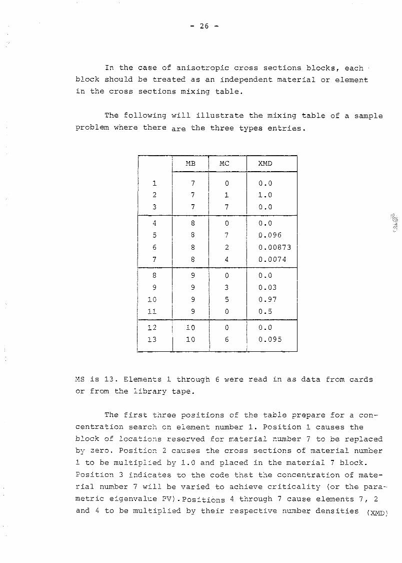
The following will illustrate the mixing table of a sample

problem where there a r e the three types entries.

1

2

3

4

5

6

7

8

9

10

11

12

13

MB

7

7

7

8

8

8

8

9

9

9

9

10

10

MC

0

1

7

01i

2

4

0

3

5

0

0

6

XMD

0.0

1.0

0.0

0.0

0.096

0.00873

0.0074

0.0

0.03

0.97

0.5

0.0

0.095

MS is 13. Elements 1 through 6 were read in as data from cards

or from the library tape.

The first three positions of the table prepare for a con-

centration search on element number 1. Position 1 causes the

block of locations reserved for material number 7 to be replaced

by sero. Position 2 causes the cross sections of material number

1 to be multiplied by 1.0 and placed in the material 7 block.

Position 3 indicates to the code that the concentration of mate-

rial number 7 will be varied to achieve criticality (or the para-

me trie eigenvalue PV) . Positions A- through 7 cause elements 7, 2

and 4 to be multiplied by their respective number densities (XMD)

- 27

and combined to form the macroscopic material number 8. In a

similar manner, material number 9 is constructed of elements

3 and 5. The position 11 causes the macroscopic cross sections

of material 9 to be multiplied by a number, that might correspond

to a volume fraction. Positions 12 and 13 calcúlate the macrosco-

pic cross sections of element 6 and place them in material 10.

In other example is assumed that we are searching for

an enrichment and wish to maintain the total mass constant,

x.u «25 . ,T28 ,T25 . ,T28then: N1 + N = N_ + N_ .

N1 and N ? are the initial and final concentrations respectively,

for U and U materials.

N- = EV . N1

28 28N_ = f(EV) . N1 ; f(EV) is a function depending on EV.

N25 + N^8 = EV . N f + f (EV) . N28

f(EV) -

Leta ;

(1N f

' N ? 8 )

N 2 5

- EV N fNf

8 - -N f

For the particular case of 1SL = N : a=2.0 and 8 = -1.0

f(EV) = 2.0 - EV

The table would be like:

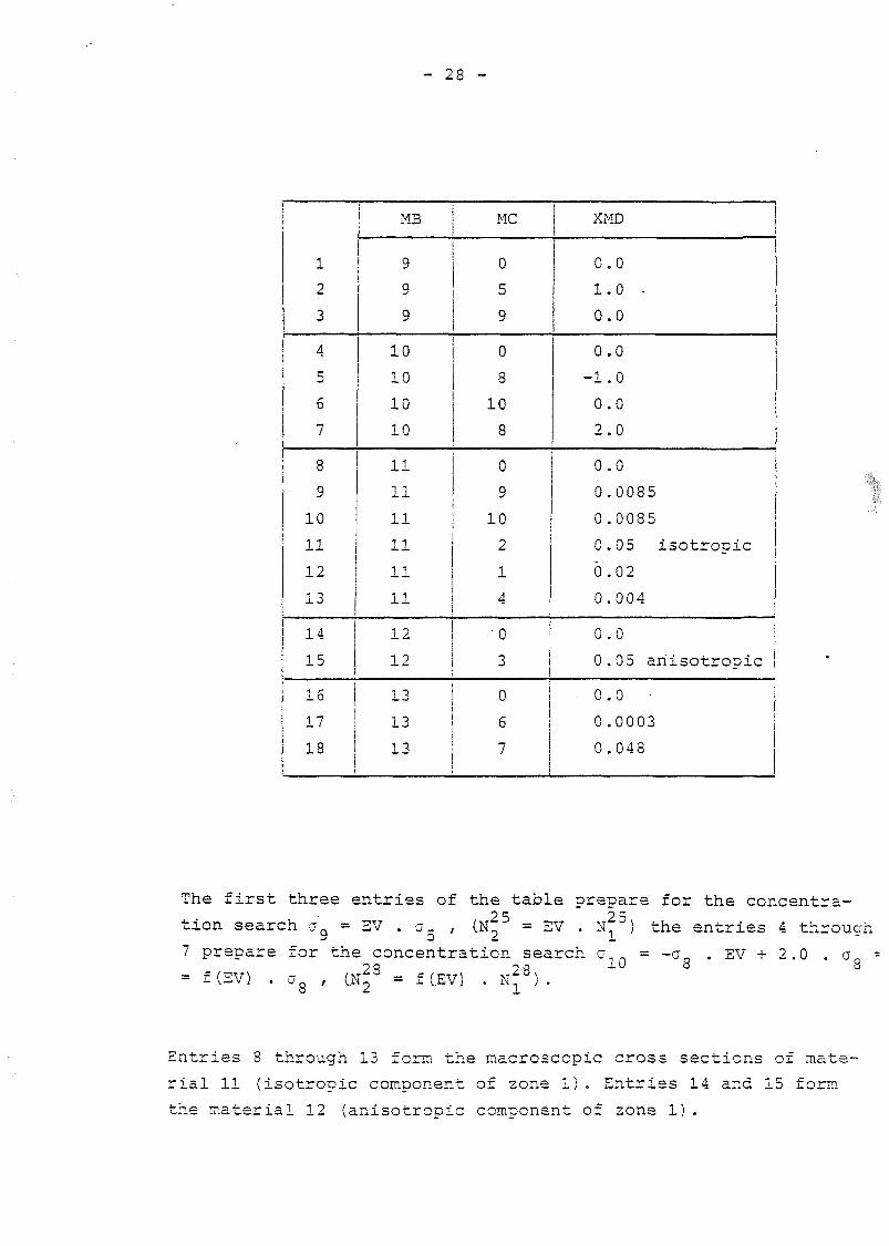
- 28 -

1

2

3

4

5

6

7

O

9

10

11

12

13

14

15

16

17

18

\

MB

9g

9

10

10

10

10

11

11

1111

11

11

12

12

13

13

13

MC

0

5

9

0

8

10

8

0

9

10

2

1

4

•o3

0

6

7

XMD

0.0

1 . 0 •

0.0

0.0

-1.0

0.0

2.0

0.0

0.0085

0.0085

0.05 isotropic

6.02

0.004

0.0

0.05 ariisotropic

• 0 . 0

0.0003

0.048

The first three entries of the table prepare for the concentra-

the entries 4 through

EV + 2 .0 . a „ ••

tion search a = EV (N ° = SV7 prepare for the concentration search c = -o

= f(EV) . c8 , CN^8 = f(EV) "28s

8'1

Entries 8 through 13 form the macroscopic cross sections of mate-

rial 11 (isotropic component of zone 1) . Entries 14 and 15 forra

the material 12 (anisotropic component of zone 1).

- 29 -

The elements 2 and 3 are the isotropic and anisotropic

components respectively of the same element. Entries 16 through

18 form the material of zone 2. Than the MZ entries will be:

-11, 13 (two zcnes), the material 11 and 12 are associated to

the first zone, and the material 13 to the second zone.

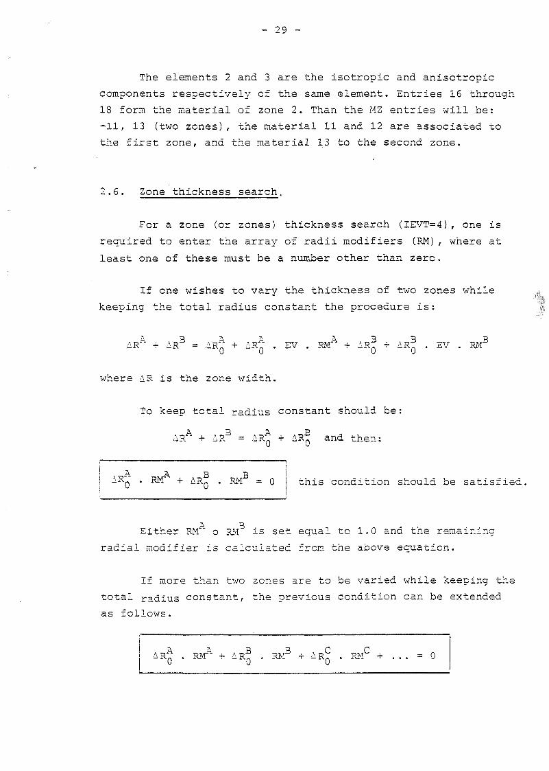
2.6. Zone thickness search..

For a zone (or zones) thickness search (IEVT=4), one is

required to enter the array of radii modifiers (RM), where at

least one of these must be a number other than zero.

If one wishes to vary the thickness of two zones while

keeping the total radius constant the procedure is:

a. 3 A A ^ 3 B BáR + MC = AR" + AR" . EV . RM" + LBZ + iíRZ . SV . RM

0 u u 0

where AR is the zone width.

To keep total radius constant should be:

A 3 A 3_iR" + AR = AR" -f- AR and then:

* 3 3 '. RM* + A.RQ . RM = o i this condition should be satisfied,

Either RM"" o RM" is set equal to 1.0 and the remaining

radial modifier is calculated from the above equation.

If more than two zones are to be varied while keeping the

total radius constant, the previous condition can be extended

as follows.

A R R C C

+ A RQ . RM + ARJ . RM + ... = 0

- 30 -

And ratios (n-2) of the radii modifiers must be knovm, .

where n is the number of zones to be varied. For example if three

zones are to be varied, ©xther A/B, A/C or B/C must be known.

Setting either A, B or C equal to 1.0 the remaining two

radii modifiers may be calculated.

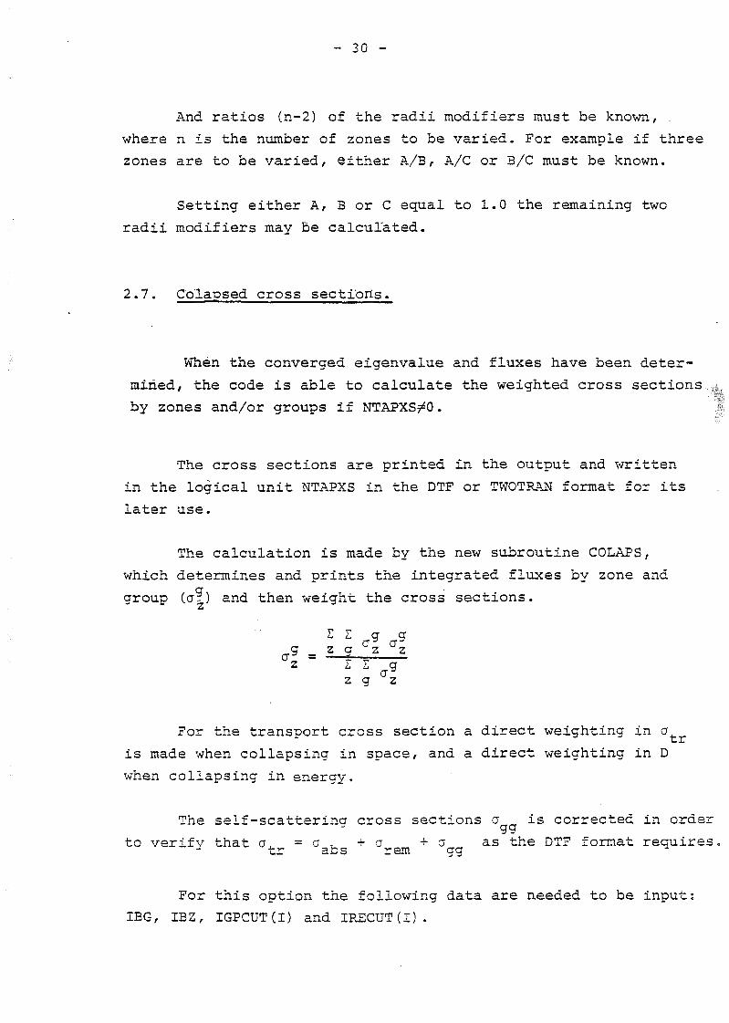
2.7. CoXapsed cross sectiorts

When the converged eigenvalue and fluxes have been deter-

miñed, the code is able to calcúlate the weighted cross sections

by zones and/or groups if NTAPXSrO.

The cross sections are printed in the output and written

in the logical unit NTAPXS in the DTF or TWOTRAN format for its

later use.

The calculation is made by the new subroutine COLAFS,

which determines and prints the integrated fluxes by zone and

group (a?) and then weight the cross sections.z

2 I g g* = z ? C* azZ " I I g

z a z

For the transport cross section a direct weighting in a

is made when collapsing in space, and a direct weighting in D

when collapsing in energy.

The self-scatterinq cross sections a is corrected in order^ gg

to verifv that a = a , + a + a as the DTF format reemires.tr abs rem gg

For this option the following data are needed to be input:

IBG, IBZ, IGPCÜT(I) and IRECÜT(I).

- 31 -

(IBG-D/2 and iBG/2 ternas will be obtained for upscattering

and downscattering respectively.

2.8. Cross sections input by tape.

The cross sections records on binary tape to be read when

MTP>0 are two for each material. The first one is the title

(LD(I),I = 1,72), and from LD(38) to LD(42) is the material number

in octal basis, that transformed to decimal basis, should be com-

pared to the Identification materials nuiabers MTT on cards, which

are desired to be read.

The second record is:

(XKI(I) ,I=1,IGM) , (VE(I) ,I=1,IGM), ( (CS (I,J,NE) ,I=1,IHM) ,J=1,IGM)

it contains the fission spectrum, the group speeds and the cross

sections tables.

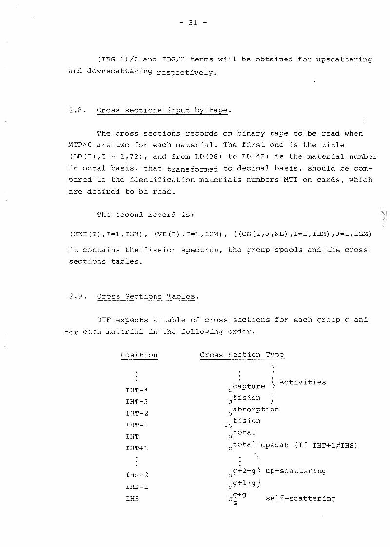
2.9. Cross Sections Tables.

DTF expects a table of cross sections for each group g and

for each material in the following order.

Position Cross Section Type

IHT-4 acapture

IHT-3 afision

IHT-2 aabsorption

IHT-1 va f Í S Í O n

IHT a t o t a l

I H T + 1 fftotal upscat (If IHT+lÎHS)

I H S_ 2 ag+2^g> up-scattering

IHS-I jIHS a5^5 self-scattering

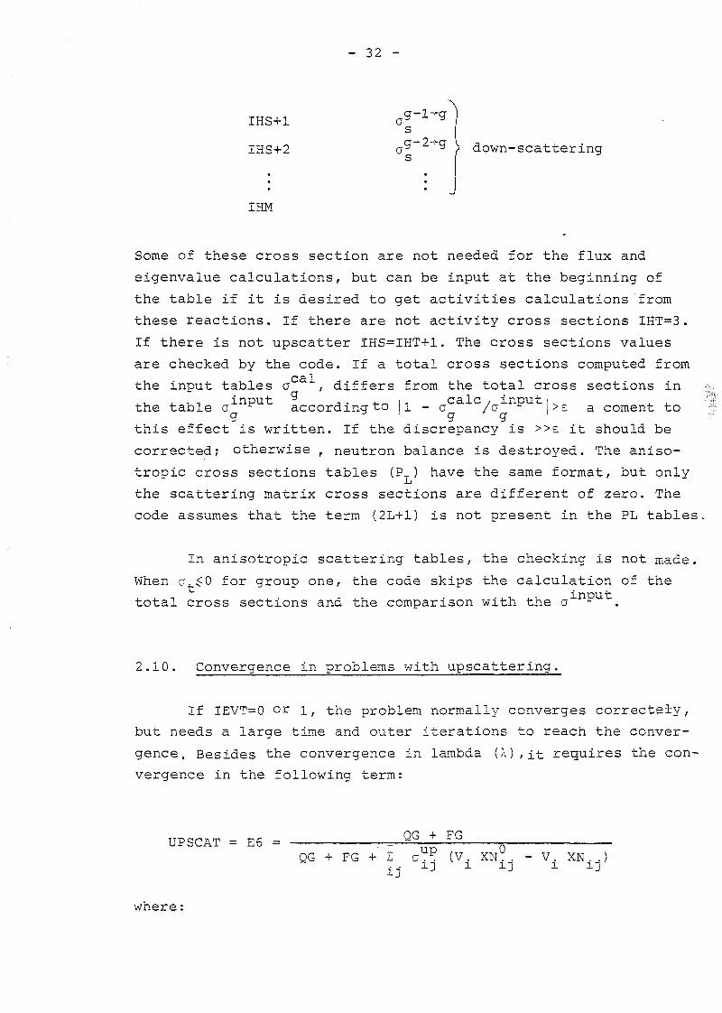
- 32 -

IHS+1s

IHS+2 a_ g \ down-scattering

IHM

Some of these cross section are not needed for the flux and

eigenvalue calculations, but can be input at the beginning of

the table if it is desired to get activities calculations from

these reactions. If there are not activity cross sections IHT=3.

If there is not upscatter IHS=IHT+1. The cross sections valúes

are checked by the code. If a total cross sections computed fromcalthe input tables a , dxffers from the total cross sections in

, , , , , input ^ , . i-~ ¡ * cale , input i. , ,the taole a - according to ± - c /a *• \>e a coment to

g g g

this effect is written. If the discrepancy is >>e it should be

corrected; otherwise , neutrón balance is destroyed. The aniso-

tropic cross sections tables (P_) have the same format, but only

the scattering matrix cross sections are different of zero. The

code assumes that the term (2L+1) is not present in the PL tables,

In anisotropic scattering tables, the checking is not made.

When o,$0 for group one, the code skips the calculation of the

total cross sections and the comparison with the a

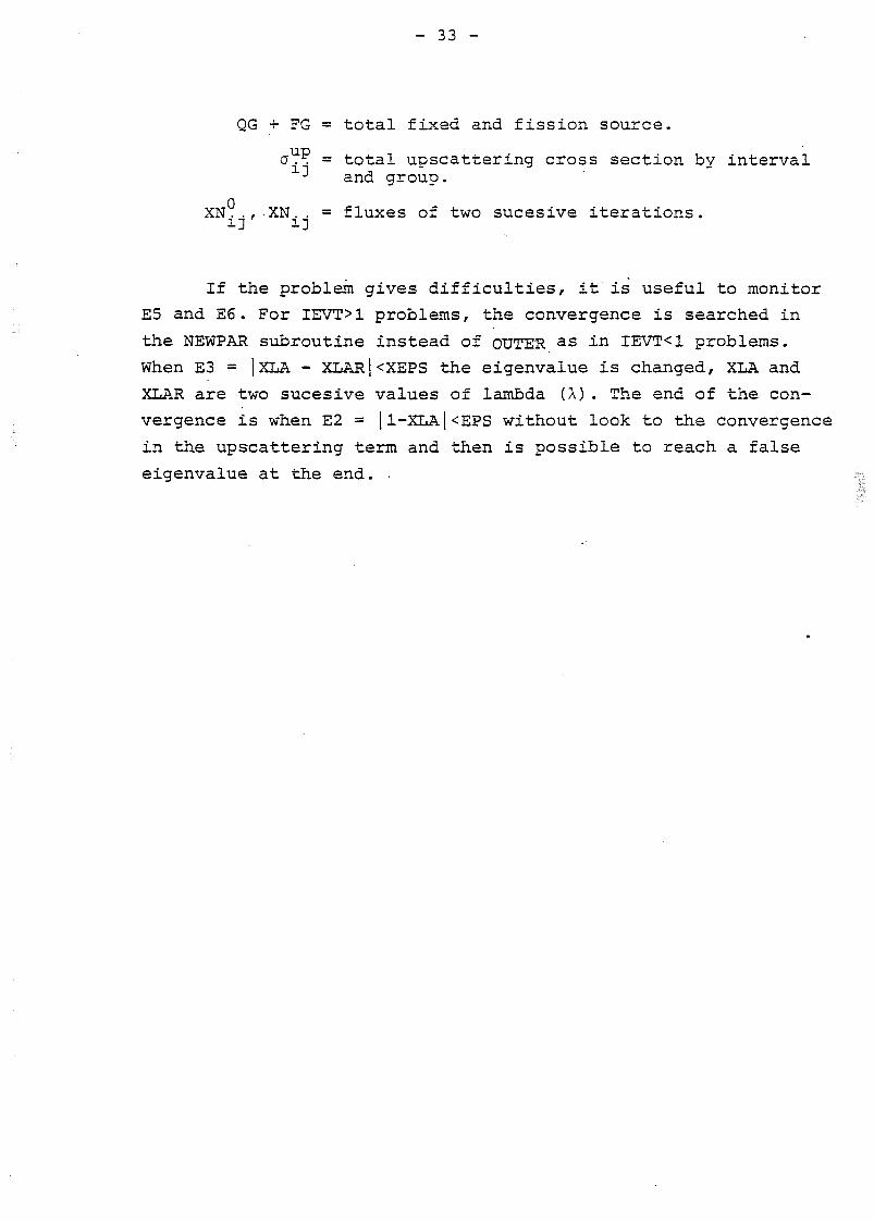
2.10. Convergence in problems with upseattering.

If IEVT=0 or i, the problem normally converges correctely,

but needs a large time and outer iterations to reach the conver-

gence. Besides the convergence in lambda {X) , it retjuires the con-

vergence in the following term:

UPSCAT = E6 = - ^ Q G + F G

OG + FG + I GUÍ? (V. XN° . - V. XN. .)

wnere:

- 33 -

QG + FG = total fixed and fission source.

a^? = total upscattering cross section by interval-1 and group.

XN. ., -XN. . = fluxes of two sucesive iterations.13' 13

If the problem gives difficulties, it is useful to monitor

E5 and E6. For IEVT>1 problems, the convergence is searched in

the NEWPAB. subroutine instead of OUTER as in IEVT<1 problems.

When E3 = JXLA - XLAR|<XEPS the eigenvalue is changed, XLA and

XLAR are two sucesive valúes of lambda (A). The end of the con-

vergence is when E2 = |l-XLA|<EPS without look to the convergence

in the upscattering term and then is possible to reach a false

eigenvalue at the end. ,

- 34 -

3. OUTPUT DESCRIPTION (1'2)

3.1. input data.

3.2. Microscopic and macroscopic cross sections (If IDf'lOO!

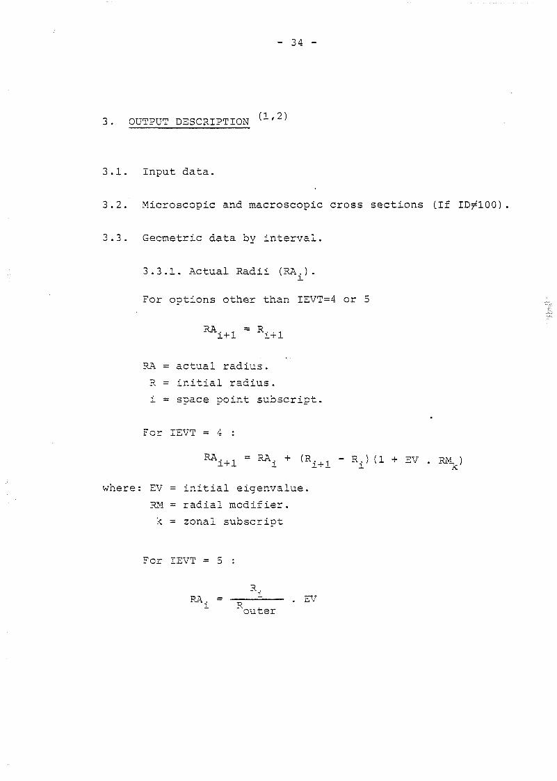
3.3. Geometric data bv interval.

3.3.1. Actual Radii (RA.).

For options other than IEVT=4 or 5

1+1 1+1

RA = actual radius.

R = initial radius.

i = space point subscript.

For ISVT = 4 :

RA. = RA + (R. - R. ) (1 + SV

where: EV = initial eigenvalue.

RM = radial modifier.

k = zonal subscript

For ISVT = 5 :

Ri

RA.. = — = . SV*outer

- 35 -

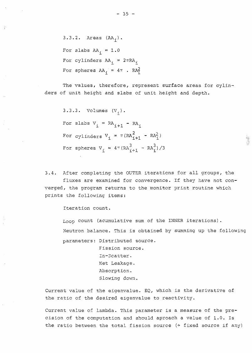
3 . 3 . 2 . Áreas (AA.).

For s l abs AA. = 1.0i

For cy l inde r s AA. = 2TTRA.

For spherss AA. = 4TT . RA?

The valúes, therefore, represent surface áreas for cylin-

ders of unit height and slabs of unit height and depth.

3.3.3. Volumes (V.).

For slabs V. = RA.,, - RA.i í + l i

For cylinders V± =

For spheres V. = 4TT(RA^+1

3.4. After completing the OUTER iterations for all groups, the

fluxes are examined for convergence. If they have not con-

verged, the program returns to the monitor print routine which

prints the following items:

Iteration count.

Loop count (acumulative sum of the INNER iterations).

Neutrón balance. This is obtained by sununing up the following

parameters: Distributed source.

Fission source.

In-Scatter.

Net Leakage.

Absorption.

Slowing down.

Current valué of the eigenvalue. EQ, which is the derivative of

the ratio of the desired eigenvalue to reactivity.

Current valué of lambda. This parameter is a measure of the pre-

cisión of the computation and should aproach a valué of 1.0. Is

the ratio between the total fission source (+ fixed source if any)

- 36 -

at the end and at the beginning of the outer iteration.

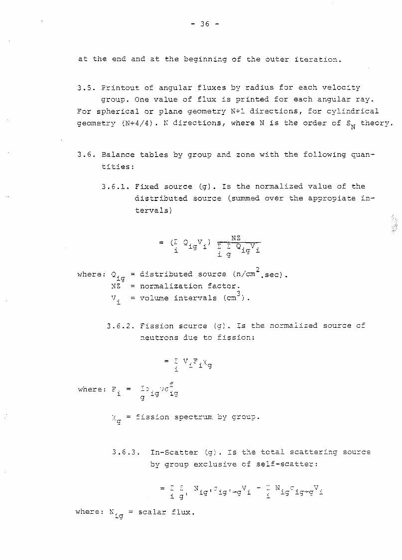
3.5. Printout of angular fluxes by radius for each velocity

group. One valué of flux is printed for each angular ray.

For spherical or plañe geometry N+l directions, for cylindrical

geometry (N+4/4). N directions, where N is the order of S~ theory

3.6. Balance tables by group and zone with the following quan-

tities:

3.6.1. Fixed source Cg)- Is the normalized valué of the

distributed source Csummed over the appropiate in-

tervals)

= ti Q. V.) . TUZ

n .-

where: Q. = distributed source (n/cm msec) .xcr

NZ = normalization factor.V. = volunte intervals Ccm ) .

3.6.2. Fission scurce (g). Is the normalized source oj

neutrons due to fission:

, i xxg

where: F. = -ó. vc~.1 a i g

X = fission spectrum by group.

3.6.3. In-Scatter Cg). Is the total scattering soures

by group exclusive of self-scatter:

, ig1 ig'-g i i xg xg-g x

where: N.. a = sea lar flux.

- 37 -

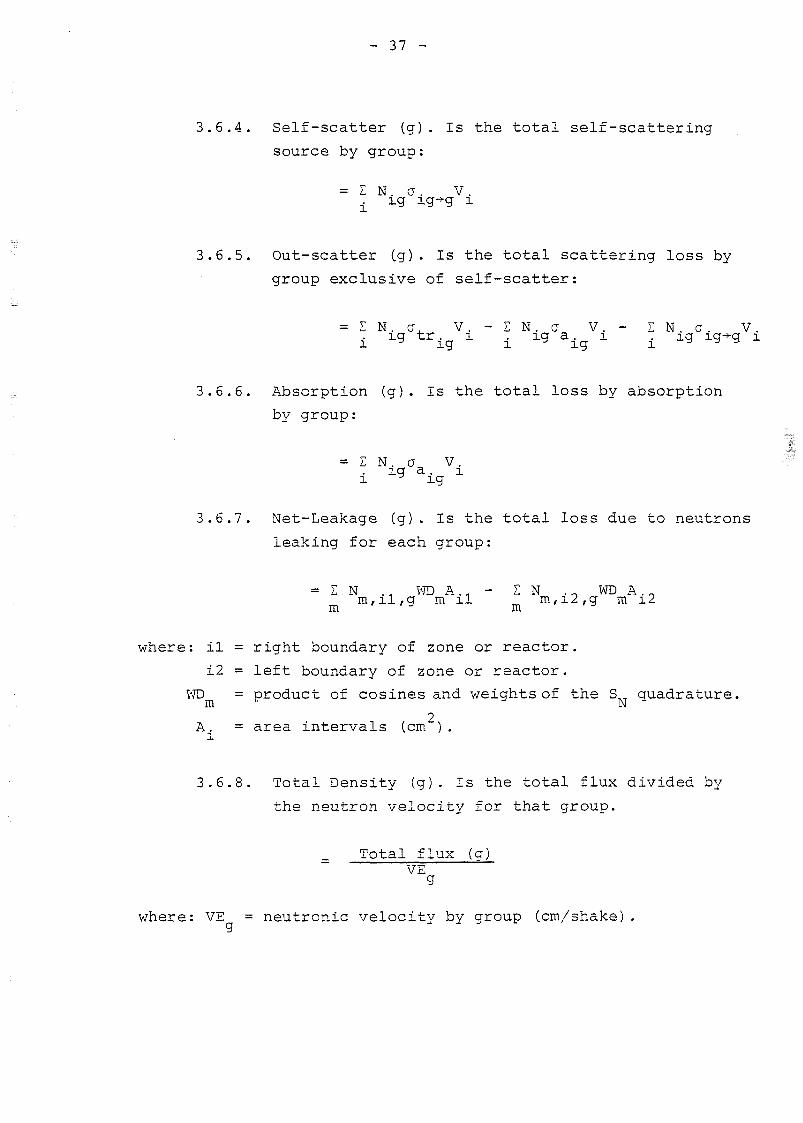
3.6.4. Self-scatter (g). Is the total self-scattsring

source by group:

= E N. a. V.i ig xg->g i

3.6.5. Out-scatter (g). Is the total scattering loss by

group exclusive of self-scatter:

= E N. a. V. - Z N. a V. - Z N. a. Vi ^ trig X ± ig a±g X i ^ ^ ^

3.6.6. Absorption (g). Is the total loss by absorption

by group:

= E N. a V.xg a . xx y xg

3.6.7. Net-Leakage (g). Is the total loss due to neutrons

leaking for each group:

= Z N .. TO A.. - E N . _ WDA._m,xl,g m xl m,x2,g m x2

where: il = right boundary of zone or reactor.

i2 = left boundary of zone or reactor.

WD = product of cosines and weights of the S_ auadrature,

2A_. = área intervals (cm ) .

3.6.8. Total Density (g). Is the total flux divided by

the neutrón velocity for that group.

Total flux (g)VE

g

where: VE = neutronic velocity by group (cm/shake)

- 38 -

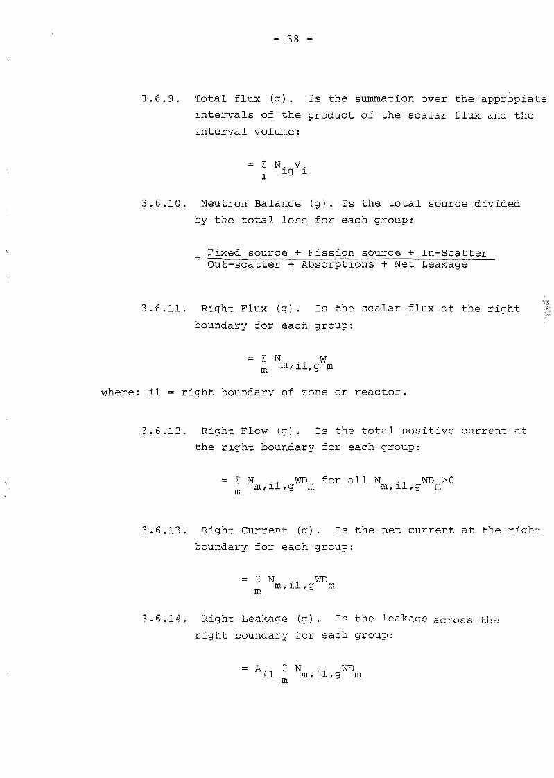
3.6.9. Total flux (g). Is the summation over the appropiats

intervals of the product of the scalar flux and the

interval volume:

= S N. V.. ig i

3.6.10. Neutrón Balance Cg)• Is the total source divided

by the total loss for each group:

Fixed source + Fission source 4- In-ScatterOut-scatter + Absorptions + Net Leakage

3.6.11. Right Flux (g). Is the scalar flux at the right

boundary for each group:

m ni/il,g m

where: il = right boundary of zone or reactor.

3.6.12. Right Flow (g). Is the total positive current at

the right boundary for each group:

= Z N .. WD for all N .. WD >0m,xl,g m m,il,g m

3.6.13. Right Current (g). Is the net current at the right

boundary for each group:

= I N ., WDm,il,g m

3.6.14. Right Leakage (g). Is the leakage across the

right boundary for each group:

= A., I N ... WDil mfil(5 mm

- 39 -

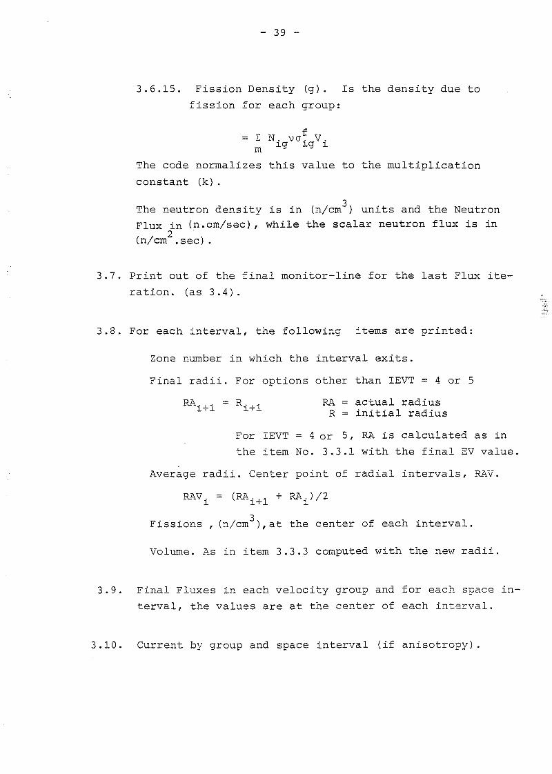
3.6.15. Fission Density (g). Is the density due to

fission for each group:

= S N. vaf V.m ig ig x

The code normalizes this valué to the multiplication

constant (k).

The neutrón density is in (n/cm ) units and the Neutrón

Flux in (n.cm/sec), while the scalar neutrón flux is in

(n/cm .sec).

3.7. Print out of the final monitor-line for the last Flux ite

ration. (as 3.4).

3.8. For each interval, the following items are printed:

Zone number in which the interval exits.

Final radii. For options other than IEVT = 4 or 5

RA - = R. .. RA = actual radiusx+x x+x R _ i n i t i a l

For IEVT = 4 or 5, RA is calculated as in

the item No. 3.3.1 with the final EV valué,

Average radii. Center point of radial intervals, RAV.

RAVi = (RAi+1 + RAi)/2

Fissions , (n/cm ), at the center of each interval.

Volume. As in item 3.3.3 computed with the new radii.

3.9. Final Fluxes in each velocity group and for each space in-

terval, the valúes are at the center of each interval.

3.10. Current by group and space interval (if anisotropy).

- 40 -

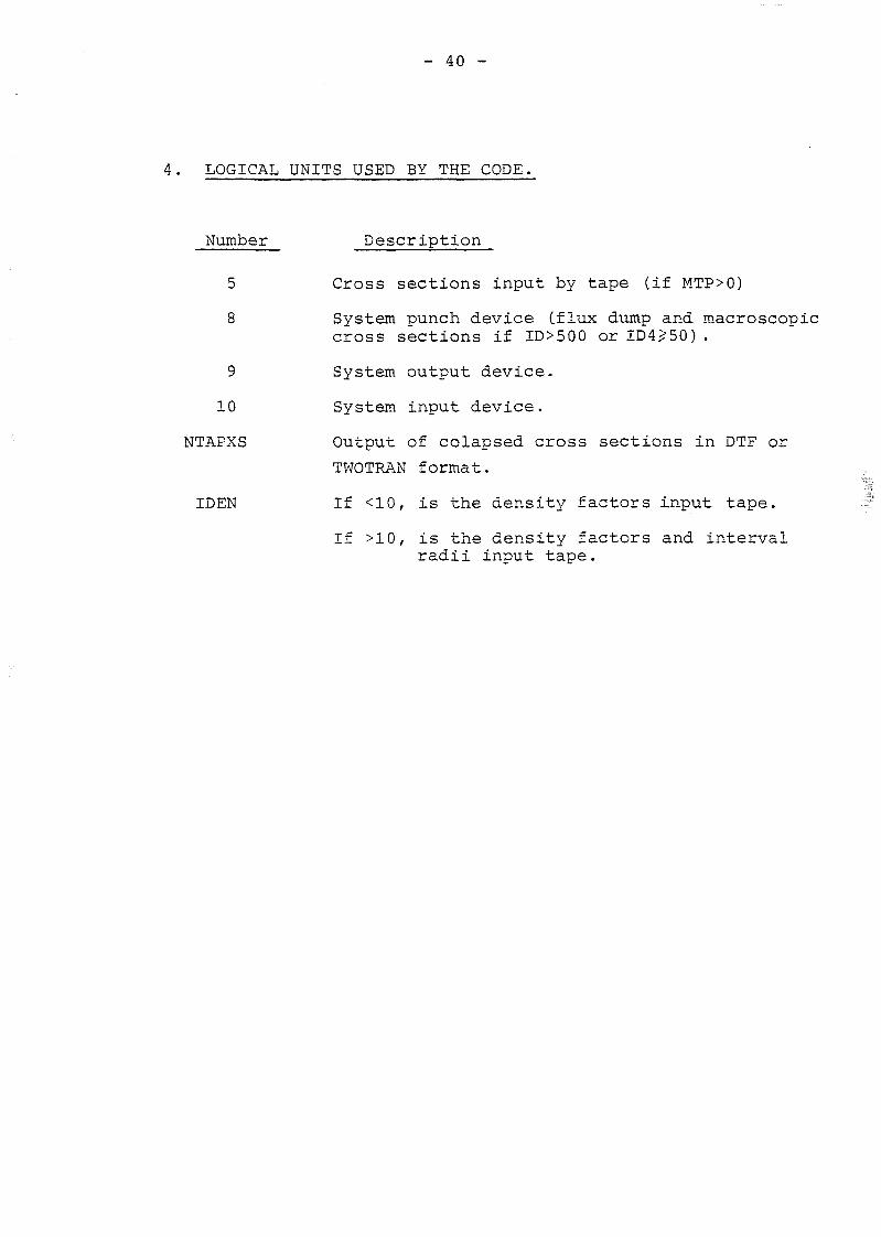
4. LOGICAL UNITS ÜSED BY THE CODE.

Number Description

5 Cross sections input by tape (if MTP>0)

8 System punch device (flux dump and macroscopiccross sections if ID>500 or ID4>50).

9 System output device.

10 System input device.

NTAPXS Output of colapsed cross sections in DTF or

TWOTRAN f orina t.

IDEN If <10, is the density factors input tape.

If >10, is the density factors and intervalradii input tape.

- 41 -

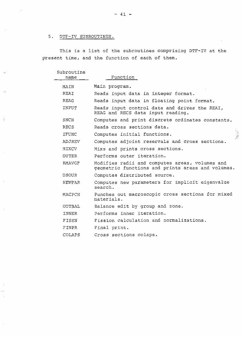
5. DTF-IV SUBROUTINES.

This is a list of the subroutines comprising DTF-IV at the

present time, and the function of each of them.

Subroutineñame

MAIN

REAI

REAG

INPUT

SNCN

RECS

IFUNC

ADJREV

MIXCV

OUTER

RMAVGF

DSOUR

NEWPAR

MACPCH

OUTBAL

INNER

FISSN

FINPR

COLAPS

Function

Main program.

Reads input data in integer format.

Reads input data in floating point format.

Reads input control data and driv.es the REAI,REAG and RECS data input reading.

Computes and print discrete ordinates constants.

Reads cross sections data.

Computes initial functions.

Computes adjoint reserváis and cross sections.

Mixs and prints cross sections.

Performs outer iteration.

Modifies radii and computes áreas, volumes andgeometric functions and prints áreas and volumes,

Computes distributed source.

Computes new parameters for implicit eigenvaluesearch.

Punches out macroscopic cross sections for mixed

materials.

Balance edit by group and zone.

Performs inner iteration.

Fission calculation and normalizations.

Final print.

Cross sections colaps.

- 42 -

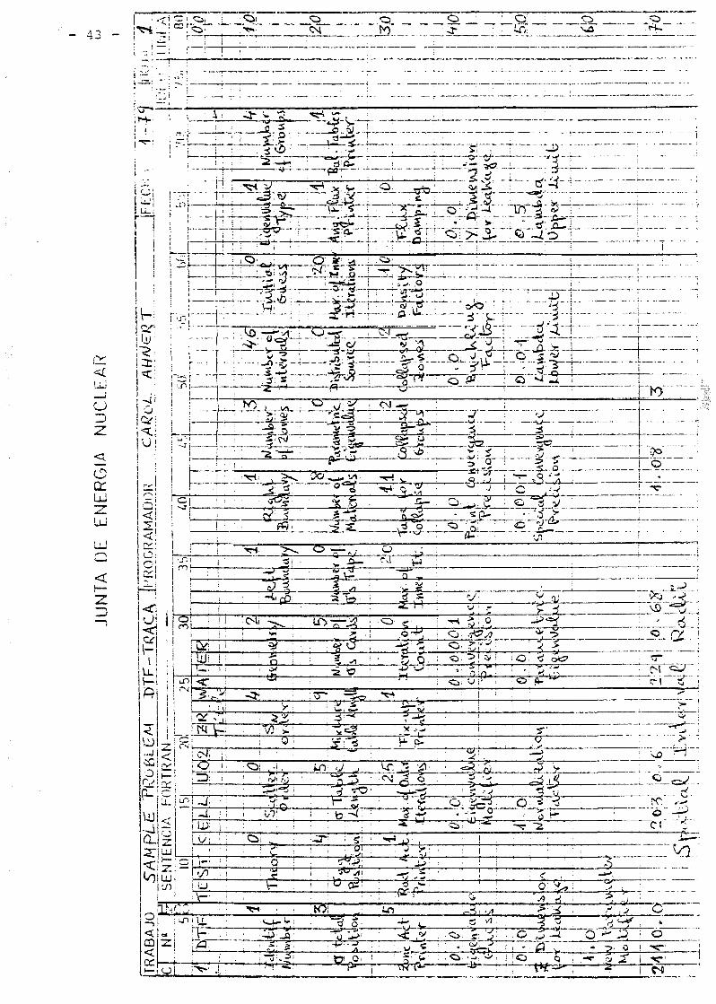
6. SAMPLE PROBLEM INPUT DATA.

In this chapter, there are the input data sheets to be

punch on cards for a sample problem, a cylindrical cell of ura-

nium oxide, zirconium ciad and moderated by light water.

These sheets will help to fill the sheets for other cases

getting a general overview of the data sequences.

•

j

i

ri

1

Ii

í

í

¡

O

z:

JER

(;

UJ

1

—)

—i

\ J • -

U_¡

~>

i:• < ;

- J 1

O'

'O

c

AM

A

0

( ^

iU.w-

D-j

sC

O

Q_2~< -

1

0

ÂB

A

;

i

1i1

ii

1|

1i

•

ii

i

¡ - y

vi:

i íñ1

1^«4

• • 1

Lo}

>

. íL

- ; 7-. t

ri

I7v

vi "

O<D

1 O")

¡

j

!Ií

¡ un

1

I1

!

1 ' .

O !

§^—;_

i

•

. - —

—

- —

—

•

•

¡

\ — •

< : •

(

! N i V

oJi' O

1 -Ji - * ;

! 1¿>:

;í * * " '

^ —

.]_. _ O;

- \ ; ' • — —

- t — i — — • . - • * - - • -

: ; ^ : « r - .; '• . - ^ v ^ "

; : : Vrn ', . 1 • <y v

1 ... | ; u ) ' ' ! ;

; : , O ; • ; :

! '• '^l tí!i '•; • i ÍJ5¡ % • r

_;.• j { . ? 1

""" * ^ - ^ -

r. ' • 5:9«-2 ; 0

\ "z "ir

f :

¡ C^íí - ^ :

¡ ; • 3 •

• n •:

^; •• : 3 ü !

; Q '<'• ' :

Oí . -i .

• •*" O¡ l , v O ! ~

i : Ci í • :

; i : C' i : 0 :

! . .j

! -2

• j v ¡ *

j ' ~ ! ; " ^ •

• - - -

.

- ~ ^

•^+ ^ .

* * * •

: * c<.

0 * :

-::J-

. .)

O- ' ;

* " f -

!

o1 ;

V

(530 _ ,

•V=>

O -—i

1

<2•2

-p; T

_¿

¡ • fe

i ü

iO i

, ,ü

1 ; \p

V I

- ^ •

V—

te, ;

"Ü? ;5 • '

O ;J\ '•

"O :

•¿ .

• ^ 0 '

;•• s "

:--Í: ;

• S i •

..Bi •

D-^ír";

" ÍJ> • :

Q. !

. 0 .

.

0 .

í\l

• O

uT<N

^»-

—

—

-

—

—

- '—

— 4

C :

0

^L0

o -

V

g' y

O-><

s.

X

"-í

- *

-x-

y •>¿>

v' :MJi—

< y

O '

' , - 1

0•_>

_ T

- f. «û0-

V^1

0

•4-»

^ !

> •

_o _ __

—*55*-

•O: ?*• >j—i ' : • •

-—-oks—ri- ^:-;

«y, ;

- 51- ;0 £° i

—_i

• * • • / > •

O, .-J

^ .)

- - ¿ p - •

•V-

• -o. 3 ! cy ¡.: * ; , * "

"O, ' ^ i1' •

!

1

!

*¿! .•=A ! Ai

S : • *

' ! :

; ' 1 i

1

>>

»-•$> ' /1

^ - .S' '¿:

O . •-<• ' ^ '

i-.-H

i • C

"•J

>--J

O "¡i

S*ü

0

- ¿3

—

.

" - -

•4-

—t

tra . -.'«»

-*a—

V

tí*

V

u

—i.

_a.

— -

.. —

_

—,

0 ' " -2 (

• • ^ o¡ •"*" 5 • ¿"i ¡

_cs._

1

— - • • - -i

1

O•

!

í

- J :

- ^ 1

C I vj

¿* •

•>• '

^ -

>

O . - ^

re ••-•0 -—'C( " í "

u—

0O

es


SENTENCIA FORTRAN -

JUNTA DE ENERGÍA NUCLEAR Ul

I

TRABAJOC

""' 5

i

o

IRLOSENTENCIA FORTRAN-

~~IO

0

<

til! !: i ;

i

u

26!r

U

8

>

r

e

5

30

t

AVI

. . 3

C

! 1

I Ii '

35

LVL _ • >

iO

•r

N--t

NM• i • i

so: :''Ji!

0

ÍÍ

¡ M i -i !

1 1

i !

-¡ !

i :

! i ¡ !

¡ i

i

7i:-¡ü'.'i i I l h | _ A

7 8 0

- • »

4 A.i

¡

I i i

I í

r !- i • - - ; -

¡ i ¡

'! I

-4-i--

14

Í4-I

i I i !I ! ! ¡

1 ! I

I I | • I• ' I t • 1 -1 ! ' l !

II

Ii

• ¡ . i !

1 i

! I /; ! I Sí

' i I : '—í—,—,—i-.

Ii

I •

; i ¡¿21

!

¡

1 i

- 46 -

O

c_Ld__üJ

üJ

_ - - _ _ . . — . 1 _ _ . . . ^ . _ . * . . - _ . . . .

i V ^ : v •* • ^ i í

I •—

¡ O

__-_Ol_4 _N__L_ 4 ^ .A '•• : : - i • .•-.U—A- ^ i

• .n i -"3 /

-M ^..._

-f; L_Q.

----•*2-í-ísr

_ L . . _ . ._.

i -•

-ro-

_&._H¡¡. - ->• -i _U. -

__ ' r .....i •; _j-._.

T-fíf- T F

^ j O | O1

1l í . £fi-4—

a._Q_

JLi-J.

ooo' "__ • _r d '•J- - r • O- \_'-^-

___. i..

TC"".0¿.

u in0/

i^1 CfS: Í Q

:rzx-.-¿.- Cl

r~3

ITí' *A \O" rr

o- • ü ;

-O_{-

TM—r

; ^ ' S- rO

* mi

y: Q n i xr- ~»• < _ - - -

_P_ fri-r-y ro

; T1 I ' ¿» , 1 , . ,||H^

: N : __J.• ; c S / •

fe i <^~bN . ^ ^ ü - 1

N _ »- A . - — —.

f _ !D¡ M) vi- T E T ^" ^ i : O! ; - . i is;

1 c

iñ <N¡

1 :!/ > •

L P i

TTT

ÍUJÍluí i

• o

O í -XA—

70~i . O: ri

<— J

tal :

~Z.; •-• . í

1 «t

, - — - •

i . H -i ' *'

•• i . _ r

Z^1 i ' ^ \—t I f(^ í,

i «! -r

• 1

— l '

^ O ;

• : 5 .

¡i

i

\

> f !


TRABAJOc'

...

...f*'ÜÍM? AMANOJ JFJLQSENTENCIA FORTRAN

f— z

10

21

ií

20!

C'V

r ' •>«" •>

IA

c

C'V

I

• i

30

fiA/

: i 'i !

O1/05

U

H

X

I I ! I

i I ! ii •

i

7 i •!! I

I !! I

¡!";i :•' I I b f A

' / • ; , Gü

-l-l i

: i

I • !

i !

t !

! i ¡I ¡ i: i

i í ij !

i

» • i >•

! í t

i i

. i i i •

i i ¡ ¡ •: i I ,

! í I I • ¡i i i

- 48 -

7. REFERENCES.

(1) B.G. CARLSON, W.J. WORLTON, W. GUBER and M. SHAPIRO ,

"DTF Users Manual", United Nuclear Corporation, Report

UNC Phys/Math 3321, Vol. I and II (1963).

(2) W.W. ENGLE, M.A. BOLING and B.W. COLSTON. "A one-Dimensional,

Multigroup Neutrón Transport Program", Atomics International

Rough Draft. NAA-SR-10951 (1965).

(3) K.D. LATHROP, "DTF-IV, a Fortran-IV. Program for Solving

the Multigroup Transport Equation with Anisotropic Scattering"

LA-3373 C1945) .

(4) G. MINSART, J. QUENON, "Some Improvements to the stability

and the Convergence of the Reactor Codes DTF-IV, EXTERMINA-

TOR and TREPAN-TRIBU". Numerical Reactor Calculations IAEA

(1972) .

(5) B.G. CARLSON and C E . LEE, "Mechanical Quadrature and the

Transport Equation". LAMS-2573 (1961).

(6) K.D. LATHROP and B.G. CARLSON, "Discrete Ordinates Angular

Quadrature of the Neutrón Transport Equation", LA-3186 (1965).

(7) B.G. CARLSON, "Transport Theory: Discrete Ordinates Quadra-

ture over the Unit Sphere", LA-4554 (1970).

(8) B.G. CARLSON, "Tables of Equal Weight Quadrature EQ Over

the ünit Sphere". LA-4734 (1971).

(9) K.D. LATHROP,"Discrete Ordinates Methods for the Numerical

Solution of the Transport Equation". Reactor Technology.

Vol. 15, No. 2 (1972).

CIO) Handbook of Mathematical Functions, NBS. Appl. Math. Sci.

55, USGPO. Washington, pp. 916-919 (1969) .

(11) C E . LEE, "The Discrete S^ Aproximation to Transport

Theory". LA-2595 (1962).

_ 49 -

(12) F. BRINKLEY, K.D. LATHROP, Listing of the DTF-71 code, (1971;

(13) Letter from K.D. LATHROP (4 January 1974) .

(14) Handbook of Mathematical Functions - Abrawowitz and Stegun.

(15) M. GÓMEZ ALONSO. "CAPELO program". JEN Internal report.MEMO TCR/CD/7 5-02.

(16) J.P. PENAL, P.J. ERICKSON, W.A. RHOADES, D.B. SIMPSON,

M.L. WILLIAMS, "The Generation of a Computer Library for

Discrete Ordinates Quadrature Sets." ORNL-TM-6023 (Septem-

ber 1977).

(17) R.G. SOLTESZ, R.K. DISNEY, J. JEDRUCH, S.L. ZEIGLER,

" Two-Dimensional, Discrete Ordinates Transport Techniques",

WANL-PR(LL)-034, Vol. 5. August 1970.

(18) G. VELARDE, C. AHNERT, J.M. ARAGONÉS, "Analysis of the

Eigenvalue Equations in k,A,y and a Applied to Some Fast

-and Thermal- Neutrón Systems". Nuc.Sci.Eng. 66, 284 (1978).

J . E . N . 4 4 8

Jjirta de Energía Nuclear. Sección de Teoría y Cálculo de Reactores. Madrid."The neutrón transport code DTF-Traca user's manuali

and input data".AHNERT, C. (1979) 49 pp. 18 r e f s .

This is a user's manual of the neutrón transport code DTF-TRACA, which is a versión

of the original DTF-IV with some modifications otada at JEN. A detailed input data des-

cr ipt ion is given. The new options developped at JEN are included too.

INIS CLASSIFICATION AND DESCRIPTORS: E21. D codes. Manuals. Neutrón transport. Discrete

ordinate method. One dimensional calculations. Neutrón transport theory.

J . E . N . 4 4 8

Junta de Energía Nucluar- Sección de Teoría y Cálculo de Reactores. Madrid.

"The neutrón transport code DTF-Traca user1 s manual!and input data".

AHNERT, C. (1979) 49 pp. 18 reís.

This is a usor's manual of the neutrón transport code DTF-TRACA, which is a versión

of the original DTF-IV v/ith some modifications nade at JEN. A detailed input data des-

cr ipt ion is given. The now options developped at JEN are included too.

INIS CLASSIFICATIÜN AND DESCRIPTORS: E21. D codes. Manuals. Neutrón transport. Discrete

ordinate method. One dimensional calculations. Neutrón transport thoory.

J . E . N . 4 4 8

Junta de Energía Nuclear. Sección de Teoría y Cálculo de Reactores. Madrid."The neutrón transport code DTF-Traca user's manual!

and input data".AHNERT, C. (1979) 49 pp. 18 r e f s .


of the original DTF-IV with some modifications made at JEN. A dotailed input data des-

criptions is given. The new options developped at JEN are included too.

INIS CLASSIFICATION AND DESCRIPTORS: E21. D codes. Manuals. Neutrón transport. Discrete


_ _ _ _ _ _ _ _ _ _ _ _ _ _ _ i

J.E. N. 448

Junta de Energía Nuclear. Sección do Teoría y Cálculo de Reactores. Madrid.

"The neutrón transport code DTF-Traca user's manualand input data".

AHNERT, C. (1979) 49 pp. 18 refs.


of the original DTF-IV with some modifications made at JEN. A detailed input data des-

criptions is given. The new options developped at JEN are included too.

INIS CLASSIFICATION AND DESCRIPTORS: E21 - D codes. ñanuals. Neutrón transport. Discrete


J . E . N . 448

Junta de Energía Nuclear. Sección de Teoría y Cálculo de Reactores. Madrid.

" E l código ele t ranspor te neut ron ico D T F - T r a c a " .AIIICRÍ, C. (1979) 49 pp. 18 reís. . ' • •

Es un manual de usuario del código de transporte neutronico DTF-TRACA, esta es una

versión del DTF-IV original con algunas modificaciones introducidas en la JEN. Se descri-

be de forma detallada la entrada de datos del código, así como las nuevas opciones intro

ducidas.

CLASIFICACIÓN INIS Y DESCRIPTORES: E2I. D codes. Hanuals. Neutrón transport. Discreto

ordinate metbod. One dimensional calculations. Neutrón transport theory.

J . E . N . 448


"El código de transporte neutronico DTF-Traca".AHNERT, C. (1979) 49 pp. 18 refs.


versión del DTF-IV original con algunas modificaciones introducidas en la JEN. Se descrí-¡

be de forma detallada la entrada de datos del código, así como las nuevas opciones intro-¡

ducidas.

CLASIFICACIÓN INIS Y DESCRIPTORES: E21. D codes. Hanuals. Neutrón transport. Discrete

ordinate method. One dimensional calculations. Neutrón transport' theory.

J . E . N . 448


"El código de transporte neutronico DTF-Traca".

AHNERT, C. (1979) 49 pp. 18 refs.


versión del DTF-IV original con algunas modificaciones introducidas en la JEN. Se descri-¡

be de forma detallada la entrada de datos del código, así como las nuevas opciones intro-¡

ducidas.

CLASIFICACIÓN INIS Y DESCRIPTORES: EZl. D codes. Manuals. Neutrón transport. Discrete

ordinate mothod. One dimensional calculations. Neutrón transport theory.

J . E . N . 448


"El código de transporte neutronico DTF-Traca".AHNERT, C. (1979) 49 pp. 18 r e f s .


versión del DTF-IV original con algunas modificaciones introducidas en la JEN. Se desen

be de forma detallada la entrada de datos del código, así como las nuevas opciones intro

ducidas.

CLASIFICACIÓN INIS Y DESCRIPTORES: E21. D codos. Manuals. Neutrón transport. Discrete


Documents

JUNTA DE ENERGÍA NUCLEAR - IPEN · y Publicaciones, Junta de Energía Nuclear, Ciudad Uni-versitaria, Madrid-3, ESPAÑA. Las solicitudes de ejemplares deben dirigirse a este mismo