24.05.2017 Kapitel 3 1

Kapitel 3: Dynamic Programming

Inhalt:

• Weighted Interval Scheduling

• Segmented Least Squares

• Knapsack Problem

• Sequence Alignment

2

Knapsack Problem

Knapsack problem.

Given n objects and a "knapsack."

Item i weights wi > 0 kilograms and has value vi > 0.

Knapsack has capacity of W kilograms.

Goal: fill knapsack so as to maximize total value.

Ex: { 3, 4 } has value 40.

Greedy: repeatedly add item with maximum ratio vi / wi.

Ex: { 5, 2, 1 } achieves only value = 35 greedy not optimal.

1

Value

18

22

28

1

Weight

5

6

6 2

7

Item

1

3

4

5

2W = 11

3

Dynamic Programming: False Start

Def. OPT(i) = max profit subset of items 1, …, i.

Case 1: OPT does not select item i.

– OPT selects best of { 1, 2, …, i-1 }

Case 2: OPT selects item i.

– accepting item i does not immediately imply that we will have to

reject other items

– without knowing what other items were selected before i, we don't

even know if we have enough room for i

Conclusion. Need more sub-problems!

4

Dynamic Programming: Adding a New Variable

Def. OPT(i, w) = max profit subset of items 1, …, i with weight limit w.

Case 1: OPT does not select item i.

– OPT selects best of { 1, 2, …, i-1 } using weight limit w

Case 2: OPT selects item i.

– new weight limit = w – wi

– OPT selects best of { 1, 2, …, i–1 } using this new weight limit

OPT (i, w)

0 if i 0

OPT (i 1, w) if wi w

max OPT (i 1, w), vi OPT (i 1, wwi ) otherwise

5

Input: n, W, w1,…,wn, v1,…,vn

for w = 0 to W

M[0, w] = 0

for i = 1 to n

for w = 1 to W

if (wi > w)

M[i, w] = M[i-1, w]

else

M[i, w] = max {M[i-1, w], vi + M[i-1, w-wi ]}

return M[n, W]

Knapsack. Fill up an n-by-W array.

Knapsack Problem: Bottom-Up

6

Knapsack Algorithm

n + 1

1

Value

18

22

28

1

Weight

5

6

6 2

7

Item

1

3

4

5

2

{ 1, 2 }

{ 1, 2, 3 }

{ 1, 2, 3, 4 }

{ 1 }

{ 1, 2, 3, 4, 5 }

0

0

0

0

0

0

0

1

0

1

1

1

1

1

2

0

6

6

6

1

6

3

0

7

7

7

1

7

4

0

7

7

7

1

7

5

0

7

18

18

1

18

6

0

7

19

22

1

22

7

0

7

24

24

1

28

8

0

7

25

28

1

29

9

0

7

25

29

1

34

10

0

7

25

29

1

35

11

0

7

25

40

1

40

W + 1

W = 11

OPT: { 4, 3 }value = 22 + 18 = 40

7

Knapsack Problem: Running Time

Running time. (n W).

Not polynomial in input size!

"Pseudo-polynomial."

Decision version of Knapsack is NP-complete.

Knapsack approximation algorithm. There exists a polynomial algorithm

that produces a feasible solution that has value within 0.01% of

optimum.

24.05.2017 Kapitel 3 8

Kapitel 3: Dynamic Programming

Inhalt:

• Weighted Interval Scheduling

• Segmented Least Squares

• Knapsack Problem

• Sequence Alignment

9

String Similarity

How similar are two strings?

ocurrance

occurrence

o c u r r a n c e

c c u r r e n c eo

-

o c u r r n c e

c c u r r n c eo

- - a

e -

o c u r r a n c e

c c u r r e n c eo

-

6 mismatches, 1 gap

1 mismatch, 1 gap

0 mismatches, 3 gaps

10

Applications.

Basis for Unix diff.

Speech recognition.

Computational biology.

Edit distance. [Levenshtein 1966, Needleman-Wunsch 1970]

Gap penalty ; mismatch penalty pq.

Cost = sum of gap and mismatch penalties.

2 + CA

C G A C C T A C C T

C T G A C T A C A T

T G A C C T A C C T

C T G A C T A C A T

-T

C

C

C

TC + GT + AG+ 2CA

-

Edit Distance

11

Goal: Given two strings X = x1 x2 . . . xm and Y = y1 y2 . . . yn find

alignment of minimum cost.

Def. An alignment M is a set of ordered pairs xi-yj such that each item

occurs in at most one pair and no crossings.

Def. The pair xi-yj and xi'-yj' cross if i < i', but j > j'.

Ex: CTACCG vs. TACATG.

Sol: M = x2-y1, x3-y2, x4-y3, x5-y4, x6-y6.

Sequence Alignment

cost( M ) xi y j

(xi, y j ) M

mismatch

i : xi unmatched

j : y j unmatched

gap

C T A C C -

T A C A T-

G

G

y1 y2 y3 y4 y5 y6

x2 x3 x4 x5x1 x6

12

Sequence Alignment: Problem Structure

Def. OPT(i, j) = min cost of aligning strings x1 x2 . . . xi and y1 y2 . . . yj.

Case 1: OPT matches xi-yj.

– pay cost for xi-yj + min cost of aligning two strings

x1 x2 . . . xi-1 and y1 y2 . . . yj-1

Case 2a: OPT leaves xi unmatched.

– pay gap for xi and min cost of aligning x1 x2 . . . xi-1 and y1 y2 . . . yj

Case 2b: OPT leaves yj unmatched.

– pay gap for yj and min cost of aligning x1 x2 . . . xi and y1 y2 . . . yj-1

OPT (i, j)

j if i 0

min

xi y jOPT (i1, j1)

OPT (i1, j)

OPT (i, j1)

otherwise

i if j 0

13

Sequence Alignment: Algorithm

Analysis. (mn) time and space.

English words or sentences: m, n 10.

Computational biology: m = n = 100,000. 10 billions ops OK, but 10 GB array?

Sequence-Alignment(m, n, x1x2...xm, y1y2...yn, , ) {

for j = 0 to m

M[0, j] = j

for i = 0 to n

M[i, 0] = i

for i = 1 to m

for j = 1 to n

M[i, j] = min([xi, yj] + M[i-1, j-1],

+ M[i-1, j],

+ M[i, j-1])

return M[m, n]

}

14

Sequence Alignment: Linear Space

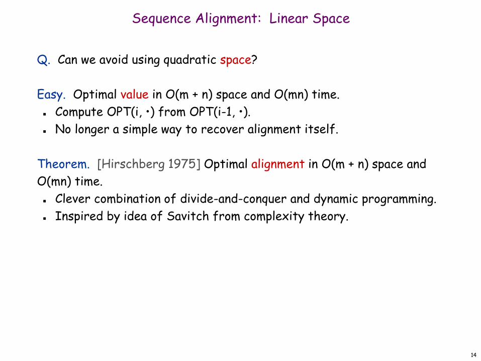
Q. Can we avoid using quadratic space?

Easy. Optimal value in O(m + n) space and O(mn) time.

Compute OPT(i, •) from OPT(i-1, •).

No longer a simple way to recover alignment itself.

Theorem. [Hirschberg 1975] Optimal alignment in O(m + n) space and

O(mn) time.

Clever combination of divide-and-conquer and dynamic programming.

Inspired by idea of Savitch from complexity theory.

15

Edit distance graph.

Let f(i, j) be shortest path from (0,0) to (i, j).

Observation: f(i, j) = OPT(i, j).

Sequence Alignment: Linear Space

i-j

m-n

x1

x2

y1

x3

y2 y3 y4 y5 y6

0-0

xiy j

16

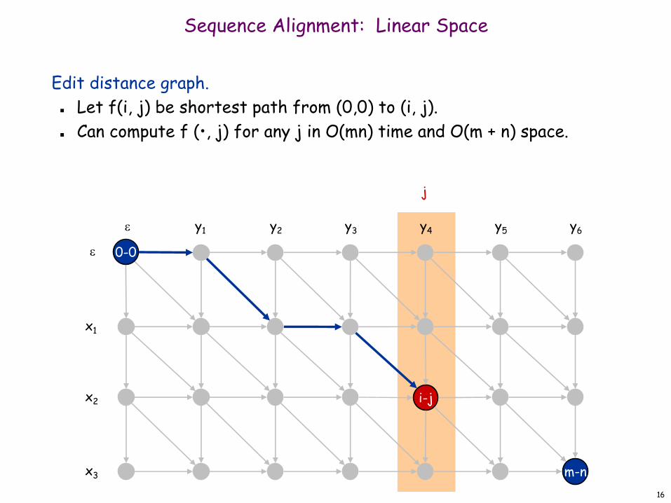
Edit distance graph.

Let f(i, j) be shortest path from (0,0) to (i, j).

Can compute f (•, j) for any j in O(mn) time and O(m + n) space.

Sequence Alignment: Linear Space

i-j

m-n

x1

x2

y1

x3

y2 y3 y4 y5 y6

0-0

j

17

Edit distance graph.

Let g(i, j) be shortest path from (i, j) to (m, n).

Can compute by reversing the edge orientations and inverting the

roles of (0, 0) and (m, n)

Sequence Alignment: Linear Space

i-j

m-n

x1

x2

y1

x3

y2 y3 y4 y5 y6

0-0

xiy j

18

Edit distance graph.

Let g(i, j) be shortest path from (i, j) to (m, n).

Can compute g(•, j) for any j in O(mn) time and O(m + n) space.

Sequence Alignment: Linear Space

i-j

m-n

x1

x2

y1

x3

y2 y3 y4 y5 y6

0-0

j

19

Observation 1. The cost of the shortest path that uses (i, j) is

f(i, j) + g(i, j).

Sequence Alignment: Linear Space

i-j

m-n

x1

x2

y1

x3

y2 y3 y4 y5 y6

0-0

20

Observation 2. let q be an index that minimizes f(q, n/2) + g(q, n/2).

Then, the shortest path from (0, 0) to (m, n) uses (q, n/2).

Sequence Alignment: Linear Space

i-j

m-n

x1

x2

y1

x3

y2 y3 y4 y5 y6

0-0

n / 2

q

21

Divide: find index q that minimizes f(q, n/2) + g(q, n/2) using DP.

Align xq and yn/2.

Conquer: recursively compute optimal alignment in each piece.

Sequence Alignment: Linear Space

i-jx1

x2

y1

x3

y2 y3 y4 y5 y6

0-0

q

n / 2

m-n

22

Theorem. Let T(m, n) = max running time of algorithm on strings of

length at most m and n. T(m, n) = O(mn log n).

Remark. Analysis is not tight because two sub-problems are of size

(q, n/2) and (m - q, n/2). In next slide, we save log n factor.

Sequence Alignment: Running Time Analysis Warmup

T(m, n) 2T(m, n /2) O(mn) T(m, n) O(mn logn)

23

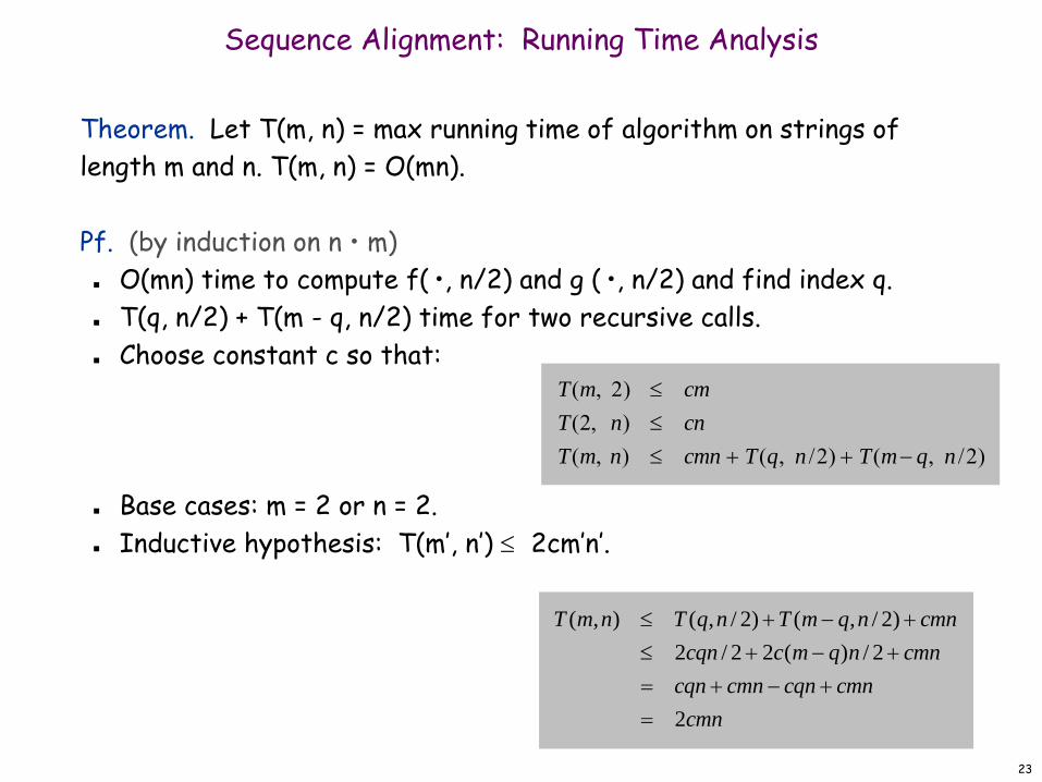
Theorem. Let T(m, n) = max running time of algorithm on strings of

length m and n. T(m, n) = O(mn).

Pf. (by induction on n • m)

O(mn) time to compute f( •, n/2) and g ( •, n/2) and find index q.

T(q, n/2) + T(m - q, n/2) time for two recursive calls.

Choose constant c so that:

Base cases: m = 2 or n = 2.

Inductive hypothesis: T(m’, n’) 2cm’n’.

Sequence Alignment: Running Time Analysis

cmn

cmncqncmncqn

cmnnqmccqn

cmnnqmTnqTnmT

2

2/)(22/2

)2/,()2/,(),(

T(m, 2) cm

T(2, n) cn

T(m, n) cmn T(q, n /2) T(m q, n /2)

24

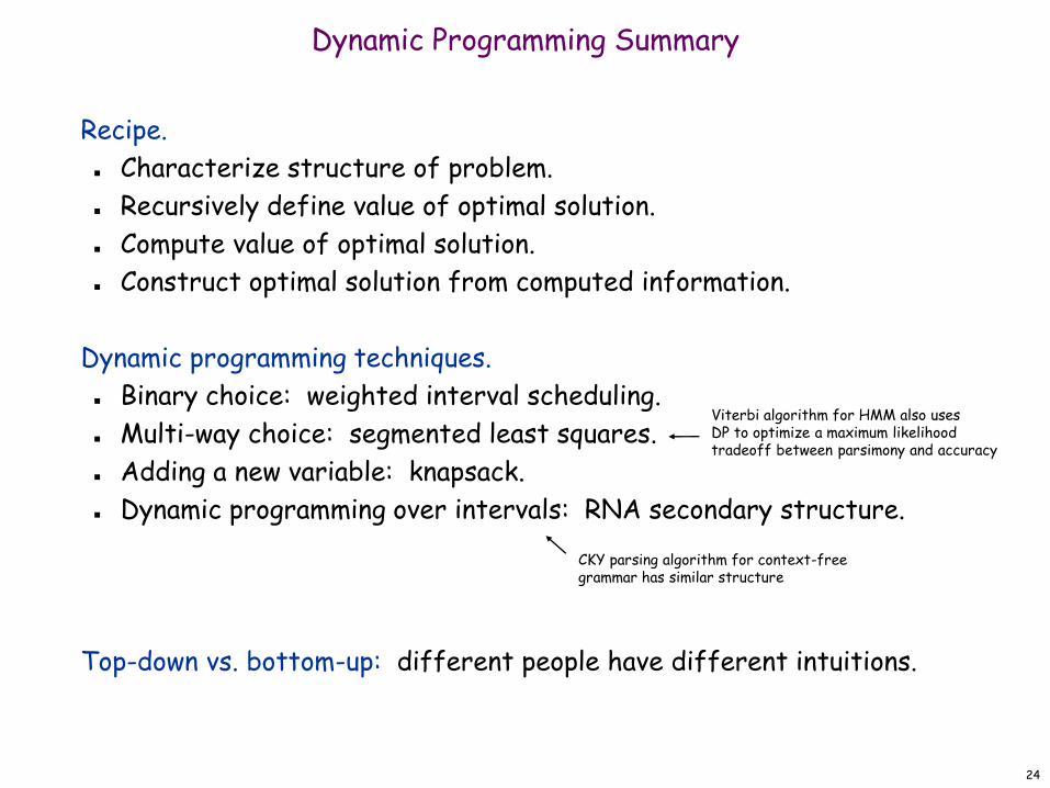
Dynamic Programming Summary

Recipe.

Characterize structure of problem.

Recursively define value of optimal solution.

Compute value of optimal solution.

Construct optimal solution from computed information.

Dynamic programming techniques.

Binary choice: weighted interval scheduling.

Multi-way choice: segmented least squares.

Adding a new variable: knapsack.

Dynamic programming over intervals: RNA secondary structure.

Top-down vs. bottom-up: different people have different intuitions.

Viterbi algorithm for HMM also usesDP to optimize a maximum likelihoodtradeoff between parsimony and accuracy

CKY parsing algorithm for context-freegrammar has similar structure

24.05.2017 Kapitel 3 25

Fragen?