Embed Size (px)
Citation preview
http://www.bgsu.edu/organizations/cfdr/main.html Phone: (419) 372-7279 [email protected]
Bowling Green State University
Work Paper Series 02-05
Kathleen A. Lamb
Gary R. Lee
2
UNION FORMATION AND DEPRESSION:
SELECTION AND RELATIONSHIP EFFECTS
Kathleen A. Lamb
And
Gary R. Lee
Bowling Green State University
Address all correspondence to: Gary R. Lee, Department of
Sociology, Bowling Green State University, Bowling Green, OH
43403-0231. Phone: (419) 372-2292. Fax: (419) 372-8306. Email:
3
Union Formation and Depression:
Selection and Relationship Effects
Abstract
Many studies have established that married people fare
better than their never-married counterparts in terms of
psychological well-being. It is still unclear, however, whether
this advantage is due primarily to beneficial effects of marriage
or to the selection of psychologically healthier individuals into
marriage. This study employs data from both waves of the
National Survey of Families and Households to test hypotheses
based on selection and relationship effects simultaneously.
Further, we differentiate union formation into cohabitation and
marriage with and without prior cohabitation. Results indicate a
very small degree of selection of less depressed persons into
marriage (but not cohabitation), and a stronger negative effect
of entry into marriage on depression, particularly when marriage
was not preceded by cohabitation.
4
Union Formation and Depression:
Selection and Relationship Effects
Introduction
A great many studies have demonstrated that married persons
fare better than the never-married on a variety of dimensions,
including global happiness (Glenn & Weaver, 1988; Lee, Seccombe,
& Shehan, 1991; Ruvolo, 1998; Stack & Eshleman, 1998); life
satisfaction and related indicators of psychological well-being
(Gove, 1972; Gove, Hughes, & Style, 1983; Gove, Style, & Hughes,
1990; Marks, 1996; Marks & Lambert, 1998; Mastekaasa, 1992, 1993,
1994; Ross, 1995); physical health (Waite, 1995); and life
expectancy (Lillard & Waite, 1995; Murray, 2000). Of particular
interest here, research has shown consistently that married
persons tend to be less depressed than the never-married
(Horwitz, White, & Howell-White, 1996; Marks, 1996; Marks &
Lambert, 1998; Ross, 1995).
Two types of explanations have been proposed for the
advantages of the married over the never-married. First is the
straightforward argument that married persons benefit directly
from their relationships with their spouses, in terms of support,
intimacy, mutual caring, companionship, and the financial
advantages that come from the pooling of resources (Gove et al.,
1990; Marks & Lambert, 1998; Ruvolo, 1998; Simon & Marcussen,
1999). A corollary to this explanation is the idea, introduced
by Pearlin and Johnson (1977), that marriage has a “buffering” or
5
“protective” effect against adverse life events or situations
such as illness, poverty, or the loss of loved ones. The marital
relationship is a social and psychological resource that helps
people better withstand loss and adversity.
Both forms of this argument imply that marriage improves
psychological well-being, either directly or by moderating the
effects of events and circumstances that would otherwise result
in lower well-being. Although this is often termed the “social
causation” explanation (e.g., Mastekaasa, 1992), we prefer to
call it the “relationship effect.”
The second type of explanation is the “selection effect,”
which postulates that happier, healthier people are more likely
to be selected into marriage (Glenn & Weaver, 1988; Horwitz et
al., 1996; Mastekaasa, 1992). The selection effect also implies
an advantage of the married over the never-married in cross-
sectional data, because those with the highest levels of well-
being would be most likely to marry, thereby raising the average
well-being of the married and lowering the average well-being of
the never-married. The selection effect does not imply change in
well-being for individuals accompanying the transition to
marriage. However, the selection effect and relationship effect
explanations are not at all mutually exclusive. The critical
question here is how much of the advantage of married persons is
attributable to each kind of effect.
While it is possible to employ cross-sectional or cohort
data to address the issue of relationship versus selection
6
effects indirectly (see Glenn & Weaver, 1988, for a particularly
compelling analysis), panel data are obviously the most useful.
Several longitudinal studies have addressed this issue. The
general consensus is that relationship effects are more powerful
and more important than selection effects, although there is some
evidence on each side.
Mastekaasa (1992) found that a measure of life satisfaction
predicted subsequent marriage for a sample of young adults in
Norway, thus supporting the selection effect. Horwitz et al.
(1996) reported that depression predicted subsequent marriage
(negatively) for women, but not men, in a sample of never-married
New Jersey residents. However, Simon and Marcussen (1999), using
the National Survey of Families and Households, observed no
differences in depression at Wave I between those who
subsequently married and those who remained single. The
longitudinal evidence on the selection effect is thus decidedly
mixed.
Evidence for the relationship effect is much stronger.
Simon and Marcussen (1999) found that those who had married by
Wave II of the NSFH were significantly less depressed than those
who remained single (recall that there were no differences
between these groups at Wave I). Marks and Lambert (1998), also
using the NSFH, discovered that those who married between waves
became less depressed while those who remained unmarried became
more depressed; they report parallel results for global
happiness. Horwitz et al. (1996) found that marriage during the
7
course of their study was associated with reductions in both
depression and reported alcohol problems.
Each of these studies, however, assumed that the transition
to marriage is a single event, and that the relevant comparison
is simply between those who marry and those who don’t. But over
half of all contemporary marriages are preceded by cohabitation,
and more than half of all adults under age 40 have cohabited at
least once (Brown, 2000; Bumpass & Lu, 2000; Bumpass & Sweet,
1989; Seltzer, 2000). Although cohabitation typically lasts for
a much shorter period of time than marriage (Bumpass & Lu, 2000;
Seltzer, 2000), it is a prelude to marriage for many and an
alternative to marriage for some.
None of the longitudinal studies mentioned above examines
either selection into cohabitation or the consequences of
cohabitation for well-being. Instead, if cohabitants are
included in the studies, they are treated as unmarried. If
cohabitation has some of the same consequences as marriage, or if
individuals are positively selected into cohabitation based on
their well-being, treating cohabitants as single would minimize
differences between the single and the married.
Some cross-sectional studies have found cohabitants to be
intermediate between never-marrieds and marrieds in terms of
psychological well-being (e.g., Kurdek, 1991). This is
consistent with the idea that cohabitation offers some of the
advantages of marriage – intimacy, support, regular sexual
relations, companionship, economical living arrangements – but
8
without the strength of commitment and full pooling of resources
marriage entails (Horwitz & White, 1998). However, cohabitation
could also be a means of obtaining the advantages of marriage
without the costs of long-term commitment, in which case it might
have positive effects on well-being equal to or greater than
those of marriage. On the other hand, there is evidence that
cohabitation is selective of those with greater financial and
personal problems (Axinn, 1992; Booth & Johnson, 1988; Brown,
2000; Bumpass & Sweet, 1989; Clarkberg, 1999), and that
cohabitants experience lower relationship quality than do married
persons (Nock, 1995), particularly if they do not have plans to
marry (Brown & Booth, 1996). This suggests that cohabitants may
have lower levels of psychological well-being.
The longitudinal evidence on the relation of cohabitation
to psychological well-being is somewhat mixed. Horwitz and White
(1998) followed their New Jersey sample through transitions to
either cohabitation or marriage, and found that those who entered
cohabiting unions were more depressed than those who married both
before and after the transition. However, the post-transition
difference disappeared under controls for gender, financial need,
and relationship quality.
Brown (2000) compared those who entered cohabiting unions
with those who married using the National Survey of Families and
Households. She found a significant reduction in depression for
those who entered marriage between waves, but not for those who
cohabited. She also found no evidence of selection effects.
9
However, her analysis compared individuals who entered cohabiting
unions with individuals who entered marital unions; she did not
include the continuously unpartnered.
This study employs data from the National Survey of
Families and Households to follow young adults who were
unpartnered at Time 1, and who had never cohabited or married,
through transitions into cohabitation and/or marriage. Because
it is the best-measured of the indicators of psychological well-
being available in the NSFH, we focus on depression as the
critical variable. We employ depression at Time 1 as a predictor
of union formation between waves, and change in depression
between waves as a consequence of union formation.
Beginning with the subsample of those who have never
cohabited or married, we use Time 1 depression to predict three
possible outcomes: (1) remaining continuously unpartnered; (2)
entering a cohabiting union; and (3) marrying, without prior
cohabitation. Because we are interested in the effects of
depression on selection into relationships, in this part of the
analysis we ignore information on relationship outcomes; in other
words, for those who entered a union between waves we are
concerned only with the initial union they entered.
The second stage of the analysis predicts change in
depression between waves based on four outcome statuses:
continuously unpartnered, cohabitation, cohabitation followed by
marriage, and marriage without prior cohabitation. In this
analysis, our intent is to examine the effects of entry into
10
unions, not union dissolution. To achieve this objective, we
eliminate cases where individuals entered and exited a union
between waves. This means that people who cohabited and broke
up, married and divorced, cohabited with multiple partners, or
cohabited with one person but married another were excluded from
the analysis.
We hypothesize that depression at Time 1 negatively
predicts selection into both cohabitation and marriage. In
addition, we expect the effect of depression on marriage to be
stronger than its effect on cohabitation. This is because
marriage entails a stronger and more permanent commitment than
cohabitation, and therefore is likely to be regarded as a more
serious and consequential decision than cohabitation; thus
depression and other selection factors should play a greater
role.
In the second stage of the analysis, we hypothesize that
those who marry between waves experience the greatest decrease in
depression, followed by those who enter and remain in cohabiting
unions. We expect those who cohabit then marry to be similar to
those who marry without prior cohabitation, because both have
made the ultimate commitment of marriage.
Methods
The Sample
Both waves of the National Survey of Families and
Households are utilized in this study. Wave I is a national
11
probability sample of 13,007 respondents, including the primary
cross-section of 9637 households and oversamples of cohabiting
couples, persons recently married, and African-Americans. Data
were collected for the first wave in 1987 and 1988. Wave II
involves re-interviews of surviving Wave I main respondents
(N=10,007) in 1992-1994, as well as interviews with the original
spouse or cohabiting partner of the respondent, and the current
spouse or cohabiting partner of the respondent if applicable.
The sample for this study is limited to persons at Wave I
who had never been married and never cohabited (classified as
"unpartnered") and were between the ages of 18 and 35, as the
normative age for marriage in the United States is the mid-
twenties for both males and females (Horwitz and White, 1991).
Individuals who cohabit or marry for the first time after age 35
are scarce, and are likely to differ from those who establish
their initial unions at more normative ages.
Wave I of the NSFH contained 1154 persons were who had
neither cohabited nor been married and were between the ages of
18 and 35. Of these, 920 (79.7%) were followed up at Wave II.
To test the selection effect, respondents’ first union
transitions were ascertained. Fifteen cases were deleted from
analyses because they contained missing data on variables related
to start dates of relationships such that it could not reasonably
be ascertained whether respondents had, for instance, cohabited
before marriage if they had done both. Another 21 cases were
deleted due to missing data on the Wave I depression scale, the
12
main predictor of Wave II marital status. This leaves 884 cases
remaining for analysis of selection into marriage. An additional
11 cases were deleted from the equation predicting selection into
cohabitation because, at Wave II, they reported inception dates
for their cohabitation relationship that were prior to the date
of the Wave I interview.
The sample was further reduced for the analysis of the
relationship effect. Of the original 920 Wave II respondents,
40 failed to answer at least 9 of the 12 items measuring
depression at one time or the other (see below), and were
consequently eliminated from the sample. Of the remaining 880,
149 respondents were deleted from this analysis because they
entered and dissolved relationships between waves. These
included 33 respondents who married but subsequently separated or
divorced; two who were married and widowed; 10 who reported
marrying more than once; 13 who cohabited with one partner but
married another; 24 who cohabited with more than one partner; and
67 who entered but subsequently dissolved a cohabiting
relationship. In addition, two respondents gave conflicting
information as to their marital status at Wave II. This leaves
729 respondents for the analysis of the relationship effect who
were either continuously unpartnered (n=407) or entered a union
they did not leave prior to Wave II. The latter category
includes 61 respondents who entered and remained in a cohabiting
union; 110 who cohabited and then married; and 151 who married
without prior cohabitation.
13
Measurement
The primary criterion variable in this analysis is
depression, measured by the 12-item version of the Center for
Epidemiological Studies Depression scale (CES-D). The 12-item
scale was developed from the original 20-item version (Radloff,
1977) by Ross and Mirowsky (1984), and was designed to have
identical psychometric properties for men and women. The items
ask how many days in the past week the respondent felt (for
example) “depressed,” “bothered by things that don’t usually
bother you,” and “that everything you did was an effort.”
Responses for each item ranged from 0 to 7; the range of the
summated scale is thus 0 to 84. The same twelve items were used
at each time. Reliability is high at both Wave I (Cronbach’s α =
.93) and Wave II (Cronbach’s α = .92).
Forty respondents who answered eight or fewer of the 12
items at either or both times were eliminated from the analysis.
For those who answered between nine and eleven items at either
time, their mean scores for the items they did answer were
substituted for the missing items.
Several socio-demographic variables measured at Wave I are
included in the analyses because of possible relations to both
depression and marital status. These include gender (male = 1);
race (dummy variables for Black, Hispanic, and other, with non-
Hispanic White as the reference category); and education in
years. Age is also measured in years, and age-squared is
14
included because marriage before or after the normative ages may
have consequences for depression. To avoid multicollinearity
problems age and its quadratic term were centered.
Physical disabilities may affect an individual’s prospects
for marriage, and may also mediate the relationship between
marital status and depression. For the Wave I data used to
predict union transitions, an index of limitations in activities
of daily living (ADLs) was constructed by summing dichotomous
responses (yes = 1) to questions asking about limitations in
ability to care for personal needs, moving around inside the
home, working for pay, performing household tasks, climbing
stairs, and walking one city block. For the analysis of Wave II
depression the concurrent measure of ADL limitations was used, in
which the items were scored from 1 (no limitation) to 3
(extensive limitation). Also, an additional item involving heavy
housework was added, resulting in an index ranging from 7 (no
limitations) to 21 (extensive limitations).
For the test of the selection effect (i.e., the prediction
of Time 2 marital status from Time 1 depression), respondent’s
income (logged to correct skewness) and employment status
(employed = 1) at Time 1 were included. In addition, a dummy
variable indicating whether a pregnancy occurred to either a
female respondent or a male respondent’s partner was created.
The test of the effect of union transitions on Time 2
depression included respondent’s education and employment status
at Time 2. Income was measured by respondent’s individual income
15
for the unpartnered, and couple income for the cohabiting and
married, and again was logged to eliminate skewness.
Procedures
Proportional hazards models, specifically competing risks
models (Allison, 1995), were employed to test the selection
effect (i.e., the effect of Time 1 depression on subsequent union
formation). The hazard of the jth event occurring for the Ith
individual at time T is:
hij(t) = lim)t→0 Pr{t ≤ T i < t + ∆ t, J i = j T i ≥ t} , j=1..3 ∆ t
In this equation, T represents the time of first union transition
for each respondent i, and J represents the different types of
union transitions (cohabitation, cohabitation followed by
marriage, and marriage without prior cohabitation). Hence, the
equation represents the hazard that a union transition T occurs
for individual i between time t and t + )t, given that the
transition is of type j, and given that the individual has
survived to at least time t without any transitions having
occurred.
As in previous studies, risk of union formation was assumed
to begin at the date of the respondents’ eighteenth birthday.
Survival time was therefore coded as date of Wave I interview (in
century months) minus date of eighteenth birthday, plus the date
16
of first union formation (or, for the continuously unpartnered,
the date of the Wave II interview) minus the date of the Wave I
interview. This sum represents total survival time of
respondents at risk of union formation. Hence, all respondents
who formed unions were censored as of the date of union
formation, with respondents remaining single considered censored
as of the Wave II interview.
Two competing risks models were computed via the SAS
system, using the same predictors. The first model takes
marriage as the marital status of interest, treating cohabitors
and unpartnered persons as censored. The second model predicts
cohabitation, with married and unpartnered persons censored.
For the test of the relationship effect (i.e., the effect
of union formation on Wave II depression), ordinary least squares
regression is employed because the criterion variable is an
interval-appearing scale. Predictors were entered in blocks,
beginning with Wave I depression and the outcome union statuses
(cohabitation, cohabitation-to-marriage, and marriage).
Subsequent blocks were entered to ascertain whether they
explained the effects, if any, of union transitions. Gender was
entered in the second block. Other socio-demographic variables
measured at Wave I (race, age, and age-squared) were entered in
the third block. These were followed by variables measuring the
respondent’s current (Wave II) situation: current education and
income, employment status, health (limitations in activities of
daily living), and number of children. In preliminary analyses,
17
interaction terms for each union transition by sex were entered
to determine whether the transitions affect men and women
differently. However, these terms did not approach significance,
so were deleted from the final model.
A Heckman two-step estimation procedure (Heckman, 1979) was
run to ascertain how socio-demographic predictors affected
selective attrition of interviewees between waves. This involves
first estimating a probit equation with inclusion at Wave II
coded as 1, and non-inclusion coded as 2. These probit estimates
were used to calculate lambda, representing the hazard of
exclusion from the Wave II interview, based on age, race, sex,
education, self-reported health, income, employment status, and
Wave I depression. However, although there was some selective
attrition based on gender, race, and other socio-demographic
factors, the probit equation predicted only about seven percent
of the variation in attrition, and the equations with and without
lambda were essentially identical. This indicates that sample
attrition between waves did not affect the results of this
analysis. Consequently the attrition measure is not included in
the analyses reported below.
Results
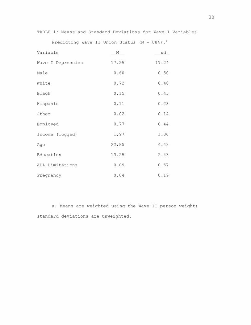
Univariate statistics for the 884 cases used to test the
effect of Wave I depression on subsequent union transitions are
reported in Table 1.
18
INSERT TABLE 1 ABOUT HERE
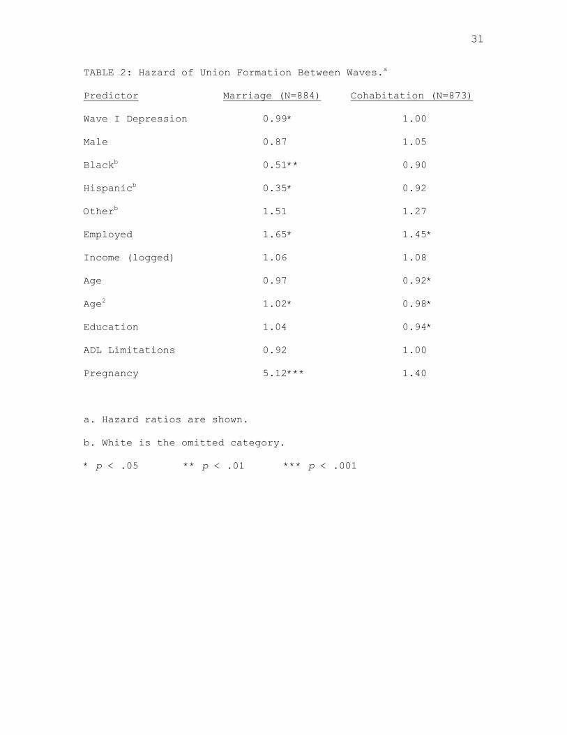
The proportional hazards analysis of the effect of Wave I
depression on the odds of marriage and cohabitation is shown in
Table 2. The coefficients in the table are hazard ratios, so
numbers less than 1 indicate a negative effect and numbers
greater than 1 indicate a positive effect. Depression indeed has
a significant negative effect on the risk of marriage, with each
increase of one point on the depression scale corresponding to a
decrease of 1 percent in the probability of marriage. This is
evidence in favor of the selection effect hypothesis. However,
the effect is certainly small. There is no effect of Wave I
depression on the probability of cohabitation.
INSERT TABLE 2 ABOUT HERE
Blacks are about 49 percent less likely to marry during the
interval between waves than Whites, and Hispanics are
approximately 65 percent less likely than Whites to marry;
neither group differs significantly from Whites on the risk of
cohabitation. Those who are employed at Wave I are more likely
to both cohabit and marry than are their nonemployed
counterparts. This could also be interpreted as evidence in
favor of a selection effect: unmarried individuals with incomes
are more desirable spouses or partners. However, income itself
is unrelated to the odds of either cohabitation or marriage. A
19
more reasonable interpretation may be that the employed are more
likely to form unions because they have completed their
educations.
Age itself is unrelated to the hazard of marriage, but the
quadratic term is positively related to marriage. This indicates
that the hazard of marriage increases with age at later ages. On
the other hand, both age and its square are negatively related to
the hazard of cohabitation, meaning that the risk of entering a
cohabiting union decreases with age at an increasing rate.
Cohabitation is considerably more common among younger persons.
Years of schooling decrease the risk of cohabitation, but do not
affect the odds of marriage. Physical health limitations are
unrelated to the risk of either marriage or cohabitation.
Pregnancy between waves substantially increases the risk of
marriage, but is unrelated to cohabitation.
There is thus some evidence for a selection effect for
marriage, in that depression marginally decreases the risk of
marriage. However, this effect is very small, and it has no
counterpart for cohabitation. Of the other variables on which
selection into marriage might be based (employment, income,
education, and physical disability), only employment influences
the odds of marriage, and this may be simply a reflection of the
fact that those who have completed their educations and thus
entered the labor force are more likely to marry. Employment
similarly increases the odds of cohabitation, but education
decreases the likelihood of cohabitation, an effect opposite to
20
what would be expected based on the selection hypothesis.
Overall, it appears that selection of the less depressed into
marriage accounts for a very small portion of the advantage of
the married.
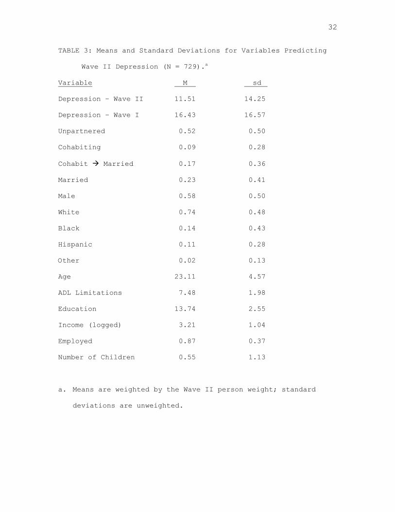
Means and standard deviations for the variables included in
the prediction of Wave II depression are shown in Table 3. It is
notable that the mean depression score at Wave II is
substantially (and significantly; p < .001) lower than at Wave I.
Clearly events or processes occurring in the interval between
waves have operated to reduce depression among sample members.
INSERT TABLE 3 ABOUT HERE
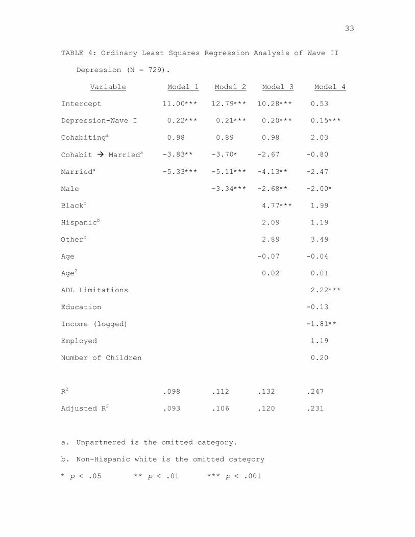
Table 4 reports the results of the OLS regression analysis
of Wave II depression, controlling for Wave I depression. The
consequence of this control is that the dependent variable is
actually change in depression between waves. Model 1 includes
the baseline depression score and the Wave II outcome statuses.
INSERT TABLE 4 ABOUT HERE
Those who entered and remained in a cohabiting relationship
do not differ on depression from the continuously unpartnered.
However, those whose cohabitations eventuated in marriage report
significantly lower depression at Wave II, and those who married
without prior cohabitation showed the greatest decrease in
21
depression compared to the unpartnered. This remains true after
gender is added in Model 2; males experienced a greater decrease
in depression than females between waves, but the effects of the
outcome statuses are not altered by the control for gender.
The socio-demographic variables race and age are added in
Model 3. Blacks experienced a greater increase (or smaller
decrease) in depression than non-Hispanic Whites between waves;
no other variable has a significant effect. The negative effect
of cohabitation followed by marriage is marginally reduced and
becomes nonsignificant. There is also a marginal reduction in
the effect of marriage without cohabitation, although it remains
significant at p < .01. The reductions occur because Blacks are
more depressed than Whites, and also less likely to marry. Some
of the apparent negative effect of marriage on depression is due
to the racial difference in marriage patterns.
Model 4 adds the variables that indicate the health,
economic, and family situations of respondents at Wave II. In
this model the effects of marriage, whether or not preceded by
cohabitation, become nonsignificant. The effect of cohabitation
followed by marriage is reduced by 79 percent from Model 1, and
the effect of marriage without prior cohabitation is reduced by
54 percent.
Two of the added variables in Model 4 have significant
effects. Limitations in activities of daily living increase
depression. However, these limitations are unrelated to union
transitions, so do not explain the effects of the outcome
22
statuses. Income, on the other hand, significantly reduces
depression and is significantly related to marriage both with (r
= .21, p < .001) and without (r = .26, p < .001) prior
cohabitation. This indicates that one reason those who marry are
less depressed than those who do not is the increased income
marriage entails. Interestingly, the bivariate correlation
between cohabitation and income, while significant, is much
smaller (r = .09, p < .05), suggesting that cohabitation without
marriage is more common among lower-income segments of the
population.
Discussion
This study is one of the few to examine the effects of
psychological well-being on union formation and the effects of
union formation on psychological well-being simultaneously. It
is also one of a very small number of studies to look at the
predictors and effects of both cohabitation and marriage. For
these reasons it provides a fairly complete picture of the
relations among depression and union formation for young adults.
Entry into a cohabitation relationship is not predicted by
Time 1 depression, nor does cohabitation have a significant
effect on Time 2 depression. Our results agree with those of
Horwitz and White (1998) and Brown (2000) that cohabitants are
more depressed than comparable married persons. We add that
entry into a cohabiting relationship appears to produce no
decrease in depression compared to remaining unpartnered.
23
Those who married between waves were less depressed at Time
2 than those who remained unpartnered or were cohabiting. This
appears, in our analysis, to be primarily a consequence of
marriage rather than of the selection of less depressed persons
into marriage. Less depressed people are indeed more likely to
marry, but the effect is small. On the other hand, those who
married between waves, particularly without prior cohabitation,
were substantially less depressed by Wave II than those who
remained unmarried. Marriage appears to have significant and
meaningful negative effects on depression.
However, the effect of marriage for those who cohabited
first was almost entirely eliminated, and reduced to
nonsignificance, by controls for other variables. In addition,
the effect of marriage without prior cohabitation was reduced by
over half and became marginally nonsignificant in our final
model. Two variables, race and income, appear to be primarily
responsible for these reductions.
Blacks were more depressed than Whites at Time 2, and also
less likely to enter either cohabitation or marriage between
waves. Inclusion of race in the equation (Model 3 of Table 4)
noticeably reduced the effects of marriage both with and without
prior cohabitation. To some degree, then, the relationship
between marriage and depression is spurious due to differing
depression levels and marriage patterns for Blacks and Whites.
(Hispanics and members of other races were more depressed than
Whites in this sample, but the effects were nonsignificant.)
24
The effect of being Black became nonsignificant in Model 4
when health limitations and income were added to the equation.
The bivariate correlation matrix (not shown) reveals that Blacks
were substantially more likely than Whites to report limitations
in activities of daily living (r = .21, p < .001) and to have
lower incomes (r = -.25, p < .001); each of these variables is
strongly related to depression. Income also mediates a portion
of the marriage-depression relationship; in part, married people
are less depressed because they are more secure financially.
This analysis does not further our understanding of why
those who cohabit prior to marriage appear to experience less of
a benefit from marriage. The negative effect of marriage on
depression is smaller for those who first cohabited in our
initial model (see Table 4), and remains smaller and becomes
nonsignificant when race enters the equation. Selection into
cohabitation as a first union has nothing to do with depression
(see Table 2). One possibility is that those who cohabited prior
to marriage have been in the relationship longer, and are
therefore more accustomed to their partnership and less excited
about it. To test this, we entered time since inception of
coresidence into Model 4 of Table 4; its effect on depression did
not approach significance (b = .03, p = .31), and the
coefficients for the union status variables did not change. This
explanation therefore appears unlikely.
A “kinds of people” explanation is also tempting,
particularly given that Table 2 implies pre-union differences
25
between those who enter cohabitation and those who enter marriage
directly on race/ethnicity, age, and education. However, Table 4
shows that the initial difference in the effects of marriage with
and without prior cohabitation (5.33 – 3.83 = 1.50) remains quite
constant as other variables are added to the model. If the
difference is due to prior characteristics of those who cohabit
versus those who marry directly, the relevant characteristics are
not included in this analysis.
Our conclusion is that marriage is associated with lower
levels of depression in young adults primarily because of
benefits of the marital relationship. Marrying is associated
with a significant and substantively meaningful reduction in
depression, particularly but not exclusively if marriage is not
preceded by cohabitation. While it is true that people who are
less depressed initially are slightly more likely than others to
marry, the effect is very small and does not appear at all for
those whose first union is cohabitation. It also appears to be
the case that some of the most important benefits of marriage, at
least according to the criterion of reducing depression, are
financial; married persons are less depressed than the
unpartnered in large part because their incomes are higher.
Further research on the properties of marriage that reduce
depression would be helpful in understanding the processes by
which the relationship effect works. Such research might also
help us understand why prior cohabitation reduces the beneficial
effect of marriage.
26
References
Allison, P. D. (1995). Survival analysis using the SAS system: A
practical guide. Cary, NC: SAS Institute, Inc.
Axinn, W. G. (1992). The relationship between cohabitation and
divorce: Selectivity or causal influence? Demography, 29, 357-
373.
Booth, A., & Johnson, D. R. (1988). Premarital cohabitation and
marital success. Journal of Family Issues, 9, 255-272.
Brown, S. L. (2000). The effect of union type on psychological
well-being: Depression among cohabitors versus marrieds.
Journal of Health and Social Behavior, 41, 241-255.
Brown, S. L., & Booth, A. (1996). Cohabitation versus marriage: A
comparison of relationship quality. Journal of Marriage and
the Family, 58, 668-678.
Bumpass, L. L., & Lu, H. H. (2000). Trends in cohabitation and
implications for children’s family contexts in the United
States. Population Studies, 54, 29-41.
Bumpass, L. L., & Sweet, J. A. (1989). National estimates of
cohabitation. Demography, 26, 615-625.
Clarkberg, M. (1999). The price of partnering: The role of
economic well-being in young adults’ first union experiences.
Social Forces, 77, 948-967.
Glenn, N. D., & Weaver, C. N. (1988). The changing relationship
of marital status to reported happiness. Journal of Marriage
and the Family, 50, 317-324.
27
Gove, W. R. (1972). The relationship between sex roles, mental
illness and marital status. Social Forces, 51, 34-44.
Gove, W. R., Hughes, M., & Style, C. B. (1983). Does marriage
have positive effects on the well-being of the individual?
Journal of Health and Social Behavior, 24, 122-131.
Gove, W. R., Style, C. B., & Hughes, M. (1990). The effect of
marriage on the well-being of adults. Journal of Family
Issues, 11, 4-35.
Heckman, J. J. (1979). Sample selection bias as specification
error. Econometrica, 47, 153-161.
Horwitz, A. V., & White, H. R. (1991). Becoming married,
depression, and alcohol problems among young adults. Journal
of Health and Social Behavior, 32, 221-237.
Horwitz, A. V., & White, H. R. (1998). The relationship of
cohabitation and mental health: A study of a young adult
cohort. Journal of Marriage and the Family, 60, 505-514.
Horwitz, A. V., White, H. R., & Howell-White, S. (1996). Becoming
married and mental health: A longitudinal study of a cohort of
young adults. Journal of Marriage and the Family, 58, 895-907.
Kurdek, L. A. (1991). The relations between reported well-being
and divorce history, availability of a proximate adult, and
gender. Journal of Marriage and the Family, 53, 71-78.
Lee, G. R., Seccombe, K., & Shehan, C. L. (1991). Marital status
and personal happiness: An analysis of trend data. Journal of
Marriage and the Family, 53, 839-844.

28
Lillard, L. A., & Waite, L. J. (1995). ‘Til death do us part:
Marital disruption and mortality. American Journal of
Sociology, 100, 1131-1156.
Marks, N. (1996). Flying solo at midlife: Gender, marital status,
and psychological well-being. Journal of Marriage and the
Family, 58, 917-932.
Marks, N., & Lambert, J. D. (1998). Marital status continuity and
change among young and midlife adults. Journal of Family
Issues, 19, 652-686.
Mastekaasa, A. (1992). Marriage and psychological well-being:
Some evidence on selection into marriage. Journal of marriage
and the Family, 54, 901-911.
Mastekaasa, A. (1993). Marital status and subjective well-being:
A changing relationship? Social Indicators Research, 29, 249-
276.
Mastekaasa, A. (1994). Marital status, distress, and well-being:
An international comparison. Journal of Comparative Family
Studies, 25, 183-206.
Murray, J. E. (2000). Marital protection and marital selection:
Evidence from a historical-prospective sample of American men.
Demography, 37, 511-522.
Nock, S. L. (1995). A comparison of marriages and cohabiting
relationships. Journal of Family Issues, 16, 53-76.
Pearlin, L. I., & Johnson, J. S. (1977). Marital status, life-
strains, and depression. American Sociological Review, 42,
704-715.
29
Radloff, L. S. (1977). “The CES-D scale: A self-report depression
scale for research in the general population.” Applied
Psychological Measurement, 1, 385-401.
Ross, C. E. (1995). Reconceptualizing marital status as a
continuum of social attachment. Journal of Marriage and the
Family, 57, 129-140.
Ross, C. E., & Mirowsky, J. (1984). “Components of depressed mood
in married men and women: The Center for Epidemiological
Studies Depression Scale.” American Journal of Epidemiology,
119, 997-1004.
Ruvolo, A. P. (1998). Marital well-being and general happiness of
newlywed couples: Relationships across time. Journal of Social
and Personal Relationships, 15, 470-489.
Seltzer, J. A. (2000). Families formed outside of marriage.
Journal of Marriage and Families, 62, 1247-1268.
Simon, R. W., & Marcussen, K. (1999). Marital transitions,
marital beliefs, and mental health. Journal of Health and
Social Behavior, 40, 111-125.
Stack, S., & Eshleman, J. R. (1998). Marital status and
happiness: A 17-nation study. Journal of Marriage and the
Family, 60, 527-536.
Waite, L. J. (1995). Does marriage matter? Demography, 32, 483-
507.
30
TABLE 1: Means and Standard Deviations for Wave I Variables
Predicting Wave II Union Status (N = 884).a
Variable M sd
Wave I Depression 17.25 17.24
Male 0.60 0.50
White 0.72 0.48
Black 0.15 0.45
Hispanic 0.11 0.28
Other 0.02 0.14
Employed 0.77 0.44
Income (logged) 1.97 1.00
Age 22.85 4.48
Education 13.25 2.43
ADL Limitations 0.09 0.57
Pregnancy 0.04 0.19
a. Means are weighted using the Wave II person weight;
standard deviations are unweighted.
31
TABLE 2: Hazard of Union Formation Between Waves.a
Predictor Marriage (N=884) Cohabitation (N=873)
Wave I Depression 0.99* 1.00
Male 0.87 1.05
Blackb 0.51** 0.90
Hispanicb 0.35* 0.92
Otherb 1.51 1.27
Employed 1.65* 1.45*
Income (logged) 1.06 1.08
Age 0.97 0.92*
Age2 1.02* 0.98*
Education 1.04 0.94*
ADL Limitations 0.92 1.00
Pregnancy 5.12*** 1.40
a. Hazard ratios are shown.
b. White is the omitted category.
* p < .05 ** p < .01 *** p < .001
32
TABLE 3: Means and Standard Deviations for Variables Predicting
Wave II Depression (N = 729).a
Variable M sd
Depression – Wave II 11.51 14.25
Depression – Wave I 16.43 16.57
Unpartnered 0.52 0.50
Cohabiting 0.09 0.28
Cohabit Married 0.17 0.36
Married 0.23 0.41
Male 0.58 0.50
White 0.74 0.48
Black 0.14 0.43
Hispanic 0.11 0.28
Other 0.02 0.13
Age 23.11 4.57
ADL Limitations 7.48 1.98
Education 13.74 2.55
Income (logged) 3.21 1.04
Employed 0.87 0.37
Number of Children 0.55 1.13
a. Means are weighted by the Wave II person weight; standard
deviations are unweighted.
33
TABLE 4: Ordinary Least Squares Regression Analysis of Wave II
Depression (N = 729).
Variable Model 1 Model 2 Model 3 Model 4
Intercept 11.00*** 12.79*** 10.28*** 0.53
Depression-Wave I 0.22*** 0.21*** 0.20*** 0.15***
Cohabitinga 0.98 0.89 0.98 2.03
Cohabit Marrieda -3.83** -3.70* -2.67 -0.80
Marrieda -5.33*** -5.11*** -4.13** -2.47
Male -3.34*** -2.68** -2.00*
Blackb 4.77*** 1.99
Hispanicb 2.09 1.19
Otherb 2.89 3.49
Age -0.07 -0.04
Age2 0.02 0.01
ADL Limitations 2.22***
Education -0.13
Income (logged) -1.81**
Employed 1.19
Number of Children 0.20
R2 .098 .112 .132 .247
Adjusted R2 .093 .106 .120 .231
a. Unpartnered is the omitted category.
b. Non-Hispanic white is the omitted category
* p < .05 ** p < .01 *** p < .001