KAUNO TECHNOLOGIJOS UNIVERSITETAS INFORMATIKOS …1808608/1808608.pdf · „Ramps“ – protokolas yra pavaizduotas 8 pav. Įtampa 0 padavinėjama laiką , po kurio seka įtampos

KAUNO TECHNOLOGIJOS UNIVERSITETAS

INFORMATIKOS FAKULTETAS

PROGRAMŲ INŢINERIJOS KATEDRA

Nerijus Paulauskas

TARPLĄSTELINIŲ PLYŠINIŲ JUNGČIŲ IMITACINIO

MODELIO KŪRIMAS IR TYRIMAS

Magistro darbas

Vadovas

Prof. H. Pranevičius

Kaunas, 2009

KAUNO TECHNOLOGIJOS UNIVERSITETAS

INFORMATIKOS FAKULTETAS

PROGRAMŲ INŢINERIJOS KATEDRA

Nerijus Paulauskas

TARPLĄSTELINIŲ PLYŠINIŲ JUNGČIŲ IMITACINIO

MODELIO KŪRIMAS IR TYRIMAS

Magistro darbas

Recenzentas

Prof. E. Bareiša

2009.05.22

Vadovas

Prof. H. Pranevičius

2009.05.22

Atliko

IFM-3/2 gr. stud.

Nerijus Paulauskas

2009.05.22

Kaunas, 2009

Summary

The work describes gap junction model imitation system formally known as the GJM (Gap

Junction Model). In this system created simulation models simulates electrophysiological

processes in gap junction channels.

The work presents gap junction models with different formal gap junction channels

specifications. Created formal models have been used in the creation of gap junction model

imitation system. The system was developed using C # programming language. System was

developed in groups of interfaces allowing passing gap junction model parameters and

voltage excitations to different types of gap junction channels

Formulated global optimization problem for the simulation results which allows approximate

imitation data to experimental data obtained from the New York, Yeshiva University, Albert

Einstein College of Medicine Laboratory.

There are presented the results of simulation models and their comparisons with the results of

experiments with different types of channels.

TURINYS

1 Įvadas ....................................................................................................................................... 1

2 Tarpląstelinių plyšinių jungčių modelio analizė ................................................................... 2

2.1 Tikslai ir siekiami rezultatai ............................................................................................ 2

2.2 Tarpląstelinės plyšinės jungtys ....................................................................................... 2

2.3 Modeliai ............................................................................................................................ 4

2.3.1 Protokolai .................................................................................................................. 5

2.3.2 2 vartų modelis ......................................................................................................... 8

2.3.3 4 vartų modelis ....................................................................................................... 14

2.3.4 6 koneksinų modelis............................................................................................... 14

2.4 Paieška ............................................................................................................................ 18

2.4.1 Globalus optimizavimas ........................................................................................ 19

3 GJM sistemos projektavimas ............................................................................................... 23

3.1 Vartotojo panaudos atvejai ............................................................................................ 23

3.2 Bendra modulių diagrama ............................................................................................. 25

4 GJM sistemos tyrimas .......................................................................................................... 32

4.1 Programinės įrangos kokybė ......................................................................................... 32

4.2 Sistemos plėtojimas ....................................................................................................... 34

5 Eksperimentai ir imitacinė sistema ...................................................................................... 35

5.1 Eksperimentų ir imitacijos palyginimas ....................................................................... 35

5.2 Globalus optimizavimas ................................................................................................ 37

5.3 Ţmogiškasis faktorius .................................................................................................... 40

6 Išvados ................................................................................................................................... 42

7 Literatūra ............................................................................................................................... 43

8 Terminų ir santrumpų ţodynas ............................................................................................ 44

9 Priedas ................................................................................................................................... 45

1

1 ĮVADAS

Darbe yra pateikta tarpląstelinių plyšinių jungčių modelio sistema formaliai vadinama GJM

(Gap Junction Model). Šioje sistemoje sukurti imitaciniai modeliai imituoja

elektrofiziologinius procesus vykstančius tarpląstelinėje plyšinėje jungtyje.

Darbe yra pateikta PJ (plyšinės jungties) formalūs modeliai su skirtingų PJ kanalų

detalizavimu. Sudaryti formalūs modeliai buvo panaudoti kuriant PJ imitacinių modelių

sistemą. Sistema sukurta panaudojant C# programavimo kalbą. Sukurta sistema grupėmis

interfeisų leidţiančių uţduoti modeliuojamos plyšinės jungties parametrus, bei plyšinių

jungčių paduodamus įtampos suţadinimus skirtingiems PJ kanalų tipams.

Suformuluotas imitacinio modelio parametrų globalaus optimizavimo uţdavinys leidţiantis

modeliavimo rezultatus maksimaliai priartinti prie eksperimentinių rezultatų gaunamų iš

sistemos uţsakovų Niujorko, Yeshiva universiteto, Alberto Einšteino medicinos koledţo

laboratorijos.

Pateikiami PJ imitacinio modelio rezultatai ir jų palyginimai su eksperimentų rezultatais prie

skirtingų kanalų tipų. Taip pat pateikiami paieškos rezultatai ir globalaus optimizavimo

paieškos kitimas laike.

2

2 TARPLĄSTELINIŲ PLYŠINIŲ JUNGČIŲ MODELIO ANALIZĖ

2.1 TIKSLAI IR SIEKIAMI REZULTATAI

Kompiuterinės imitacijos tapo naudinga realių sistemų modeliavimo dalis fizikoje, chemijoje,

biologijoje, ekonomikoje, socialiniuose moksluose ir kitose mokslo srityse. Šiuo metu yra

sukurta daug įvairių imitacinių sistemų [4], kurios imituoja realių pasaulio objektų elgsenas.

Tarpląstelinės plyšinės jungtys yra maţai ištirtos, yra daromos įvairios prielaidos, bei kuriami

teoriniai matematiniai modeliai, kurie paaiškintų ląstelių kontaktavimą plyšinėmis jungtimis.

Pagrindinis GJM sistemos tikslas yra sukurti imitacinę sistemą, kuri imituotų ląstelių

kontaktavimą plyšinėmis jungtimis ir padėtų pagrįsti daromas prielaidas apie jų kontaktavimą.

Sukurti modeliai turėtų adekvačiai atvaizduoti ląstelių sąveikavimo procesus.

2.2 TARPLĄSTELINĖS PLYŠINĖS JUNGTYS

Koneksinai (Cx) – tai baltymai, kurie formuoja tarpląstelines plyšines jungtis kontakte tarp

kaimyninių ląstelių membranų (1 pav.). Koneksinas yra pavaizduotas 2 pav. Plyšinės jungtys

leidţia sujungtoms ląstelėms perduoti elektrinius ir metabolinius signalus [1,2,3].

Kiekvienas PJ kanalas (4 pav.) sudarytas iš dviejų puskanalių (koneksonų ţr. 3 pav.), kurie

savo ruoţtu yra sudaryti iš šešių Cx koneksinų. Tarpląstelinėje sąveikoje dalyvaujančios

plyšinės jungtys gali būti homotipinės (ląstelės išreiškia tą patį Cx izotipą), heterotipinės

(ląstelės išreiškia skirtingus Cx izotipus) ir heteromerinės (bent viena ląstelė išreiškia du ar

daugiau Cx izotipus). PJ kanalai skiriasi elektriniu laidumu, selektyviu pralaidumu, įvairiomis

cheminėmis medţiagomis ir kanalų vartų jautrumu įtampai ţr. [2].

3

Koneksinai vadinami tapačiais, jeigu jie gali sudaryti funkcinius heterotipinius PJ kanalus.

Dauguma Cx porų gali sudaryti funkcines PJ, bet egzistuoja kai kurios išimtys. Pavyzdţiui: du

pagrindiniai širdies koneksonai, Cx40 ir Cx43, kurie yra ekspresuoti širdyje ir kraujagyslėse,

nėra tapatūs ir negali sudaryti funkcinių PJ kanalų ţr. [3].

1 pav. Susidariusios tarpląstelinės plyšinės jungtys

2 pav. Koneksinas

3 pav. Koneksonas

4 pav. Tarpląstelinis kanalas

Pirmos ląstelės membrana

Antros ląstelės membrana

4

Bendra PJ savybė būdinga visiems Cx koneksinams yra kanalo vartų būsenos priklausomybė

nuo įtampos. Jungties laidumas maţėja sudarius tarpląstelinės plyšinės jungties potencialą, .

Manoma, kad kiekvienas puskanalis turi du skirtingus vartų valdymo mechanizmus: lėtus,

kuris uţdaro PJ pilnai ir greitus, kuris perveda vartus į pereinamą būsena ar būsenas su

liekamuoju laidumu. Mes skaitėme, kad kiekvienas puskanalis gali būti dviejose būsenose:

atviroje su laidumu ir uţdarytoje su laidumu . Vartų valdymo mechanizmai gali skirtis

poliariškumu, tai yra vartai gali uţsidaryti arba atsidaryti, jeigu citoplazmos pusėje

potencialas didėja arba maţėja. Jeigu puskanalių vartai turi priešingą poliariškumą, vienas

poliariškumas atidarys abu puskanalius, o priešingas potencialas uţdarys abu puskanalius.

5 pav. pavaizduota pagrindinė schema, kuria buvo sudaromos perėjimo tikimybės iš [1]

literatūros straipsnio.

5 pav. Perėjimų tikimybių pagrindinė schema

2.3 MODELIAI

Sistema susideda iš lygiagrečiai sujungtų kanalų , apibūdinamų laidumu.

Kiekvienam iš jų per vienetinį diskretinį laiką yra paduodama įtampa , į kurią kanalas

sureaguoja ir suformuoja naują laidumą arba varţą. Schema yra pavaizduota 6 pav. Ţemiau

yra pateikti formalūs modelių aprašymai. Juos aprašinėjau tiesiniu agregatiniu metodu [7].

5

6 pav. Bendra modulių schema

Įtampos padavimas kiekvienu laiko momentu priklauso nuo protokolo, su kuriuo

modeliuojama. Daţniausiai yra naudojami keturi pagrindiniai protokolai: “Steps”, “Ramps”,

“Amplitude” ir “Impulse”. Kiekvienas iš jų yra aprašytas 2.3.1 skyriuje.

2.3.1 Protokolai

Protokolai yra atsakingi uţ įtampos padavimą tam tikru diskrečiu laiko momentu. Šiame

skyriuje mes aprašysime keturis uţsakovų daţniausiai naudojamus protokolus.

„Steps“ – protokolas yra pavaizduotas 7 pav. Įtampos padavimas prasideda nuo 0 įtampa kuri

laikoma laiką per kurį kanalai nusistovi iki ramios būsenos, po to paduodamas įtampos

šuolis kuris laikomas laiką. kinta nuo iki ţingsniu .

6

7 pav. „Step“ protokolo schema

„Ramps“ – protokolas yra pavaizduotas 8 pav. Įtampa 0 padavinėjama laiką , po kurio seka

įtampos kilimas nuo 0 iki , ţingsniu . Po to laukiama kol kanalai nusistovės į ramią būseną

ir paduodamas įtampos smukimas iki – .

8 pav. „Ramps“ protokolo schema

7

„Amplitude“ – protokolas yra pavaizduotas 9 pav. 0 Įtampa padavinėjama laiką po to seka

šuolių iki įtampos ir 0, kurios yra padavinėjamos laiką .

9 pav. „Amplitude“ protokolo schema

„Ramps“ – protokolas yra pavaizduotas 9 pav. Įtampa padavinėjama nuo 0 iki ir iki – ir

visos jos laikomos laiką .

10 pav. „Ramps“ protokolo schema

8

2.3.2 2 vartų modelis

Šis modelis sudarytas iš dviejų nuosekliai sujungtų vartų a ir b (11 pav.), kurių kiekvienas turi

savo kintantį laidumą. Kiekvienas vartas gali būti atviroje arba uţdaroje būsenoje.

11 pav. 2 vartų modelio struktūra

Kiekvienas kanalo vartas apibūdinamos šiais parametrais: - perėjimo konstanta

reguliuojanti varto būsenų kitimą, - įtampos jautrumo koeficientas, - įtampos

koeficientas, - atidaryto varto laidumo funkcija nuo įtampos, - uţdaryto varto

laidumo funkcija nuo įtampos.

Vartai gali būti vienoje iš dviejų būsenų: arba , kur – atviri vartai, – uţdari vartai.

Vartų būsenų kitimas vyksta diskrečiais laiko momentais , , ,

, kur - modeliavimo laiko trukmė. Vartų būsenų kitimas parodytas 12 pav. Perėjimo

tikimybės priklauso nuo vartų būsenos ir įtampos , , :

,

,

,

a b

V

9

,

,

,

.

12 pav. Vartų būsenų grafas

Vartų laidumas priklauso nuo vartų būsenos ir pridėtos įtampos :

;

Čia – varto laidumo funkcija, - varto būsena, - pridėta įtampa.

Vidutinis kanalų laidumas:

;

Čia - kanalo laidumas laiko momentu, – kanalų skaičius, - - tojo kanalo -jų

vartų laidumas.

Sudaromas modelis turi leisti paskaičiuoti sistemos laidumą laiko momentais ,

, , .

10

Agregatinis modelis

13 pav. Agregatinės sistemos schema

k

kkkkR

...211...21

2...21...21

k

k

k

k

H

2

............

2

1

...21

Agregato 0A aprašymas

1. Išėjimo signalų aibė },...,,{ 21 kyyyY

,

čia iy - išduodama įtampa, ki ,1 .

2. Vidinių įvykių aibė }''{'' 1eE ,

čia 1''e - išduodamas iy signalas, ki ,1 .

3. Valdymo sekos }{'' 1 te ,

11

čia t - laiko kitimo ţingsnis.

4. Diskrečioji agregato būsenos dedamoji )}({)( mm tVt

,

čia )( mtV

- įtampa mt laiko momentu.

5. Tolydţioji agregato būsenos dedamoji )},''({)( 1 mm tewtz

,

čia ),''( 1 mtew - signalo išdavimo pabaigos momentas.

6. Pradinė būsena 00t ,

},0{)( 0 ttz.

7. Parametrai:

RTtV ll :)(

8. Perėjimo ir išėjimo operatoriai

)''( 1eH :

)()( 11 mm tVt

,

1mm ttt,

),''( 11 tttew mm .

)''( 1eG :

)( 1mi tVy, ki ,1 .

Agregato kiAi ,1, aprašymas

1. Įėjimo signalų aibė }{ 1xX ,

čia 1x - paduodamos įtampos reikšmė.

12

2. Išėjimo signalų aibė }{ 1yY ,

čia 1y - kanalo laidumo reikšmė.

3. Išorinių įvykių aibė }'{' 1eE ,

čia 1'e - atėjo 1x signalas.

4. Diskrečioji būsenos dedamoji )}(,),({)( mjmmjm tgattSat

, 4,1j ,

čia )( mj tSa - ja

vartų būsena mt laiko momentu, )( mj tga

- ja vartų laidumas.

5. Pradinė būsena 00t ,

}0,,,,{)( 0 aaaat

6. Parametrai:

j - vartų perėjimo koeficientas, 4,1j ,

jA - vartų jautrumo koeficientas, 4,1j ,

jV0 - įtampos koeficientas, 4,1j ,

)(vGa j - atidaryto vartų laidumo funkcija, 4,1j ,

)(vGu j - uţdaryto vartų laidumo funkcija, 4,1j .


)'( 1eH :

)1)(())((,

))(())((,

)1)(())((,

))(())((,

)(

1

1

1

1

1

mjmj

mjmj

mjmj

mjmj

mj

tPuautSajeiu

tPuautSajeia

tPaaatSajeiu

tPaaatSajeia

tSa

13

4

1 1

1

11

)(

1

)(

1

)(

k mk

mj

mj

tga

tgaxtVa

utSajeitVaGu

atSajeitVaGatga

mjmjj

mjmjj

mj )()),((

)()),(()(

11

11

1

)'( 1eG :

4

1 1

1)(

1

k mk tgay

.

Agregato 1kA aprašymas

1. Įėjimo signalų aibė },...,,{ 21 kxxxX ,

čia ix - i-tojo kanalo laidumas, ki ,1 .

2. Išėjimo signalų aibė }{ 1yY ,

čia - išduodamas laidumas.

3. Išorinių įvykių aibė }',...,','{' 21 keeeE ,

čia ie' - atėjo ix signalas.

4. Diskrečioji agregato būsenos dedamoji )}(),...,(),({)( 21 mkmmm tGtGtGt ,

čia )( mi tG - i-tojo kanalo laidumas mt - laiko momentu, ki ,1 .

5. Pradinė būsena }0,...,0,0{)(,0 00 tt


14

)'( 1eH :

imimi xtGtG )()( 1

)'( 1eG :

n

tG

tG

k

imi

m1

1

)(

)(, kai 1mm tt

2.3.3 4 vartų modelis

Šis modelis sudarytas iš keturių nuosekliai sujungtų vartų a1, a2, b1 ir b2, kurių kiekvienas

turi savo kintantį laidumą 14 pav. Kiekvienas vartas gali būti atviroje arba uţdaroje būsenoj

14 pav. 4 vartų modelio struktūra

Kadangi 4 vartų modelis beveik niekuo nesiskiria nuo 2 vartų modelio, todėl aš jo plačiau

neaprašinėsiu. Jis yra identiškas 2 vartų modeliui, tik dabar yra lygiagrečiai sujungti 4 vartai.

2.3.4 6 koneksinų modelis

Šis modelis skiriasi nuo prieš tai aprašytų modelių. Kiekvienas puskanalis sudarytas iš 6

lygiagrečiai sujungtų modelių, kurių kairys ir dešinys puskanalis yra sujungtas nuosekliai (15

pav.).

a1 b2

V

a2 b1

15

15 pav. 6 koneksinų modelio struktūra

Kiekvienas koneksonas yra sudarytas iš lygiagrečiai sujungtų šešių vartų. Kiekvienas vartas

gali būti dviejose būsenose: atviroj (Angl. Open), arba uţdaroj (Angl. Closed). Tariama, kad

koneksinai yra nepriklausomi vienas nuo kito.

Agregatinis modelis

16 pav. Pagrindinė kanalų agregatinė schema

Čia:

a1

a2

a3

a4

a5

a6

b1

b2

b3

b4

b5

b6

V

16

iC , ni ,,2,1 yra i -sis kanalas, sudarytas iš lygiagrečiai sujungtų šešių koneksinų

ir nuosekliai prijungtos varţos.

Agregatas iC , ni ,,2,1 :

1. Įėjimo signalų aibė , kur – -tojo kanalo įtampa.

2. Išėjimo signalų aibė , kur – kanalo laidumas.

3. Išorinių įvykių aibė , kur – -tojo kanalo įtampos poveikis.

4. Vidinių įvykių aibė , kur – - tojo kanalo naują būseną inicijuojantis

įvykis.

5. Valdančioji seka , kur – laiko intervalas, per

kurį apskaičiuojama nauja kanalo būsena.

6. Diskrečioji agregato būsena laiko momentu mt :

Kur – i-tojo kanalo įtampa,

– kairiojo puskanalio koneksinų įtampa,

- dešiniojo puskanalio įtampa,

– kairiojo puskanalio koneksinų būsenos,

– i-tojo kanalo laidumas,

– kairiojo puskanalio koneksinų laidumai,

- dešiniojo puskanalio laidumas.

7. Agregato būsenos tolydţioji dedamoji: , kur – laiko

momentas, kurio metu apibrėţiama nauja kanalo būsena ir apskaičiuojamas laidumas.

8. Agregato pradinė būsena:

9. Perėjimų ))(( 1eH , ( )( 1eH ) ir išėjimo ( )( 1eG ) operatoriai tokie:

17

tikimybės skaičiuojamos taip:

)(

4

)(

3

)(

2

)(

1

44

33

22

11

o

o

o

o

VVA

VVA

VVA

VVA

eK

eK

eK

eK

Tada tikimybė, kad koneksinas bus atviroje būsenoje yra skaičiuojama taip:

Čia 1A - kanalo kairiojo puskanalio jautrio koeficientas;

2A - kanalo dešiniojo puskanalio jautrio koeficientas;

1oV, 2oV

18

Čia rg - dešiniojo puskanalio laidumas

,

.

2.4 PAIEŠKA

Pagrindinis sistemos uţdavinys yra pagrįsti įvairias tarpląstelinių plyšinių jungčių

kontaktavimo prielaidas pasinaudojant eksperimento bei imitacijos rezultatais. Todėl yra

svarbu automatizuoti šį procesą, tai yra pasinaudojant eksperimentiniais rezultata is surasti

imitacinės sistemos atitikmenį ir jos įėjimo parametrus.

Sistemos parametrų paieška yra labai svarbus uţdavinys šioje sistemoje. Ji padėtų pagrįsti

įvairias prielaidas ir surastų neţinomus parametrus įvairiems kanalų tipams.

Tarkime mes turime eksperimentinius nufiltruotus duomenis (17 pav., raudona kreivė) ir

imitacijos rezultatus su tam tikrais įėjimo parametrais (17 pav., mėlyna kreivė). Mums reikia

rasti imitacijos parametrus su kuriais imitacijos ir eksperimento kreivių kvadratų skirtumas

bus maţiausias.

19

17 pav. Eksperimentiniai duomenys

Į ši uţdavinį galima ţiūrėti kaip į funkcijos aproksimavimą arba tiksliau šnekant regresiją, kai

reikia surasti neţinomos funkcijos parametrus pagal taškų aibę. Mums reikia surasti maţiausią

kvadratų skirtumą tarp eksperimentinių duomenų ir imitacinės sistemos.

2.4.1 Globalus optimizavimas

Pirma problema šiam uţdaviniui spręsti yra triukšmo lygis kreivėse. Kadangi eksperimentų

rezultatai neretai būna nukraipyti, bei atsiranda įvairių netikslumų susijusių su paklaidomis,

metodais bei įranga, kuriuos naudoja eksperimentuose, todėl pradiniai eksperimento

duomenys, prieš paduodant į paieškos sistemą bus išanalizuoti bei išfiltruoti siekiant

tikslesnių paieškos rezultatų. Iš to seka, kad eksperimentinių duomenų triukšmo lygis bus

pakankamai maţas, tačiau triukšmas egzistuos ir eksperimentų ir imitacijos rezultatuose, todėl

reikia parinkti būdą jam sumaţinti. Triukšmo lygio sumaţinimas yra reikalingas, kad būtų

galima gauti tikslesnį funkcijų maţiausių kvadratų skirtumą, nes kai triukšmas bus didelis,

bus beveik neįmanoma surasti parametrų. Todėl vykdant paieška mes turėsime abiem

duomenims paskaičiuoti kvadratų skirtumą po 2 kartus. 1-as kartas sumaţinant triukšmą

pradiniuose duomenys, o 2-as kartas įvertinant paieškos rezultatą.

20

Šiai problemai spręsti galima naudoti netiesinę regresiją [6], kuri yra naudojama įvairiems

uţdaviniams spręsti statistikoje. Šiam atvejui galima naudoti „Boltzmano“ funkciją, kurią

naudoja uţsakovai analizuodami duomenis norėdami aproksimuoti funkciją:

;exp1

minmaxmin)(

)*(

111

011 VVA

GGGVa

;exp1

minmaxmin)(

)*(

222

022 VVA

GGGVb

;)()(

)(*)()(

VbVa

VbVaVF

Pasinaudodami regresija mes galėsime gauti eksperimentų ir imitacijos rezultatų funkcijas be

triukšmo ir tokių atveju galėsime tiksliau apskaičiuoti kvadratų skirtumą. Regresijos

panaudojimo pavyzdys pavaizduotas 18 pav.

18 pav. Funkcijos aproksimavimas pasinaudojus nelinijine regresija

21

Naudodami )(VF funkciją galima nesunkiai surasti jos parametrus pasinaudodami

„Levenberg–Marquardt“ algoritmu. Tačiau problema iškyla, kai pradiniai funkcijos

parametrai yra nutolę ir algoritmas nekonverguoja, tokiu atveju kvadratų skirtumas bus labai

netikslus. Naudojant šią funkciją su esamu modeliu parametrai yra surandami, tačiau yra

patobulinta funkciją, kurią galima naudoti norint aproksimuoti duomenis:

;exp*)(min 1

11

c

V

cVG

;exp*)(max 1

11

d

V

dVG

;exp*)(min 2

22

c

V

cVG

;exp*)(max 2

22

d

V

dVG

;exp1

minmaxmin)(

)*(

111

011 VVA

GGGVa

;exp1

minmaxmin)(

)*(

222

022 VVA

GGGVb

;)()(

)(*)()(

VbVa

VbVaVF

Šioje funkcijoje yra pridėtas taip vadinamas ratifikavimas (angl. Ratification), kai laidumai

kinta priklausomai nuo krintančios įtampos. Ši funkcija mūsų atveju būtų labai naudinga, nes

yra modeliai su kuriais būtų galima vykdyti regresiją, tačiau ji visai nekonverguoja ir jos

naudoti mes negalime. Todėl regresijos naudojimas triukšmui sumaţinti atkrenta.

Triukšmui nuimti taip pat galime naudoti slenkantį kablelį (19 pav.), kuris sumaţintų

triukšmą. Kaip matome iš 19 pav. Triukšmo lygis yra sumaţinamas, bet išlieka šiokių tokių

iškraipymų. Šis variantas tinka triukšmo sumaţinimui, nors ir palieka šiokį tokį triukšmą.

22

19 pav. Imitacijos rezultatai su triukšmo lygiu (mėlyna spalva) bei sumaţintu triukšmo lygiu su

slenkančiu kableliu (juoda spalva)

Paieškos vykdymui galime naudoti globalaus optimizavimo logaritmus [5]. Šie algoritmai yra

naudojami įvairiems optimizavimo uţdaviniams spręsti pvz.: Mokyklos tvarkaraščių

sudarymui, keliaujančio pirklio ir t.t. Iš šių algoritmų buvo pasiūlyta naudoti „Exkor“ ir

„Bayes“, todėl mes juos abudu ir įgyvendinome.

23

3 GJM SISTEMOS PROJEKTAVIMAS

Programinės įrangos sistemos kontekstas yra pavaizduotas 20 pav.

KompiuterisVartotojas

20 pav. Sistemos kontekstas

3.1 VARTOTOJO PANAUDOS ATVEJAI

24

21 pav. Panaudos atvejų diagrama

1 lentelė. „Importuoti eksperimentų rezultatus“ panaudos atvejis

1. Panaudos atvejis Importuoti eksperimentų rezultatus

Aktorius Vartotojas

Aprašas Eksperimentų rezultatai importuojami į sistemą

Prieš sąlyga Nėra

Suţadinimo sąlyga Vartotojas sąsajos meniu pasirinko eksperimentų importavimas

funkciją

Po sąlyga Sistema uţkrauna duomenis ir pasiruošia parametrų paieškai

2 lentelė. „Parametrų paieška“ panaudos atvejis

2. Panaudos atvejis Parametrų paieška

Aktorius Vartotojas

Aprašas Ieškomi modelio parametrai

Prieš sąlyga Importuojami eksperimentų duomenys

Sužadinimo sąlyga Vartotojas programos sąsajoje pasirinko paieškos funkciją

Po sąlyga Sistema suranda parametrus ir atvaizduoja rezultatus grafiškai

3 lentelė. „Vykdyti imitaciją“ panaudos atvejis

3. Panaudos atvejis Vykdyti imitaciją

Aktorius Vartotojas

Aprašas Vykdoma imitacija pagal įvestu parametrus

Prieš sąlyga Pasirenkamas ir uţkraunamas protokolas

Sužadinimo sąlyga Vartotojas programos sąsajoje pasirinko vykdymo funkciją

Po sąlyga Sistema vykdo imitacija ir atvaizduoja rezultatus grafiškai

4 lentelė. „Eksportuoti imitacijos rezultatus“ panaudos atvejis

4. Panaudos atvejis Eksportuoti imitacijos rezultatus

Aktorius Vartotojas

Aprašas Rezultatai eksportuojami į rezultatų failą

25

Prieš sąlyga Vykdoma imitacija arba parametrų paieška

Sužadinimo sąlyga Vartotojas programos sąsajoje pasirinko eksportuoti funkciją

Po sąlyga Sistema išsaugo rezultatus į nurodytą failą

5 lentelė. „Keisti modelio elgseną“ panaudos atvejis

5. Panaudos atvejis Keisti modelio elgseną

Aktorius Vartotojas

Aprašas Keičiama imitacinės sistemos modelio elgsena pasinaudojus

matematinėmis išraiškomis

Prieš sąlyga Uţkrautas protokolas

Sužadinimo sąlyga Vartotojas programos sąsajoje pasirinko elgsenos keitimo funkciją

Po sąlyga Sistema pakeičia esamo protokolo elgseną

6 lentelė. „Saugoti modelio elgseną“ panaudos atvejis

6. Panaudos atvejis Saugoti modelio elgseną

Aktorius Vartotojas

Aprašas Išsaugojama elgsena i nurodytą failą

Prieš sąlyga Keičiama modelio elgsena

Sužadinimo sąlyga Vartotojas programos sąsajoje pasirinko elgsenos saugojimo funkciją

Po sąlyga Sistema išsaugo elgseną

7 lentelė. „Saugoti“ panaudos atvejis

7. Panaudos atvejis Saugoti

Aktorius Vartotojas

Aprašas Išsaugojama rezultatus

Prieš sąlyga Vykdoma imitacija arba parametrų paieška

Sužadinimo sąlyga Vartotojas sąsajoje pasirinko saugojimo funkciją

Po sąlyga Sistema išsaugo rezultatus

3.2 BENDRA MODULIŲ DIAGRAMA

Kuriama sistema susidarys iš šių modulių (22 pav.):

26

„GJM.App“

„GJM.Drawings“

„GJM.Mathematics“ „GJM.Model“

„GJM.Controls“

22 pav. Bendra modulių diagrama

„GJM.Drawings“ komponentas

Klasifikacija:

Modulis

Apibrėţimas:

Komponentas yra reikalingas grafikų bei funkcijų atvaizdavimui. Jis bus pagrindinis

komponentas atvaizduojant kuriamos sistemos rezultatus.

Atsakomybės:

Komponentas skirtas grafikų braiţymui. Jis braiţys funkcijas, leis vartotojui perţiūrėti

bei išsaugoti grafikus. Taip pat jis bus vienas pagrindinių rezultatų perţiūros komponentas.

Jame bus atitinkamos funkcijos leidţiančios vartotojams patogiai analizuoti rezultatus.

Apribojimai:

27

Komponentas turi veikti „thread safe“ rėţimu, kuris neleis panaudoti jos kintamųjų

vykstant kelioms gijoms vienu metu.

Struktūra:

Išorinių komponentų šis komponentas nenaudos.

Sąveikavimas:

Komponentą naudos pagrindinė sistemos forma kuri bus atsakinga uţ visos programos

darbą. Jos klasės bus paveldimos pridedant papildomas funkcijas.

Resursai:

Resursų komponentas neturi.

Skaičiavimai:

Komponentas vykdo savo funkcijas greitai. Čia naudojami elementarūs skaičiavimai,

kurių pagalba jis gali greitai atvaizduoti didelį kiekį duomenų.

Sąsaja:

Komponentas turės vieną klasė, kuri bus naudojama pagrindinėje formoje. Jis

atvaizduos grafikus.

„GJM.Mathematics “ komponentas

Klasifikacija:

Modulis

Apibrėţimas:

Komponentas bus naudojamas matematinių išraiškų analizavimui, globalaus

optimizavimo algoritmams bei papildomiems matematiniams skaičiavimams.

Atsakomybės:

Komponentas bus atsakingas uţ įvairius uţdavinius susijusius su matematiniais

skaičiavimais bei įvairiais algoritmais.

28

Apribojimai:



Struktūra:

Išorinių komponentų šis komponentas nenaudos.

Sąveikavimas:

Komponentą naudos „GJM.App“ komponentas.

Resursai:


Skaičiavimai:

Komponentas sukompiliuoja išraiškas į tam tikrą objektą, kurio pagalba galima išgauti

tos išraiškos rezultatą. Taip pat vykdo globalaus optimizavimo algoritmus.

Sąsaja:

Komponentas sąsajos neturės.

„GJM.Model“ komponentas

Klasifikacija:

Modulis

Apibrėţimas:

Komponentas aprašo visas pagrindines struktūras bei objektus susijusius su

tarpląstelinėmis plyšinėmis jungtimis. Taip pat vykdys modelių skaičiavimus.

Atsakomybės:

Komponentas bus atsakingas uţ modelio vykdymą.

Apribojimai:

29



Struktūra:

Komponentas naudos „GJM.Mathematics“ komponentą.

Sąveikavimas:

Komponentą naudos pagrindinė programos forma.

Resursai:


Skaičiavimai:

Komponentas lygiagrečiai vykdys modelio imitaciją.

Sąsaja:

Komponentas sąsajos neturės.

„GJM.Controls“ komponentas

Klasifikacija:

Modulis

Apibrėţimas:

Komponentas bus naudojamas pagrindinės formos langų išdėstymui bei papildomiems

grafinės sąsajos komponentams.

Atsakomybės:

Komponentas atsakingas uţ formos langų išsidėstymo valdymą.

Struktūra:

Komponentas išorinių komponentų nenaudos.

30

Sąveikavimas:

Komponentą naudos pagrindinė programos forma.

Resursai:

Komponentas resursų nenaudos.

Skaičiavimai:

Komponentas skaičiavimų neatlikinės.

Sąsaja:

Komponentas turės sąsajos komponentus, kuriuose bus dedami sistemos vidiniai

komponentai.

„GJM.App“ komponentas

Klasifikacija:

Vykdomoji programa

Apibrėţimas:

Pagrindinis vartotojo sąsajos langas.

Atsakomybės:

Komponentas atsakingas uţ visos programinės įrangos vykdymą.

Struktūra:

Komponentas naudos šiuos modulius: „GJM.Controls“, „GJM.Drawings“,

„GJM.Model“, „GJM.Mathematics“.

Sąveikavimas:

Komponento niekas nenaudos.

Resursai:

31

Komponentas naudos resursų failą, kuris turės įvairius paveiksliukus naudojamus

vartotojo sąsajoje.

Skaičiavimai:

Komponentas leis skaičiavimus pasinaudodamas kitais moduliais.

Sąsaja:

Komponentas vaizduos pagrindinę vartotojo sąsają.

32

4 GJM SISTEMOS TYRIMAS

4.1 PROGRAMINĖS ĮRANGOS KOKYBĖ

Sudarant programinės įrangos kokybės tyrimą svarbiausia reikia suformuluoti tikslus.

Kadangi modelių imitavimas susijęs su dideliais skaičiavimais, kurie gali įtakoti kitus

veiksmus su šia programine įranga tokius kaip parametrų paieška, todėl reikia įsitikint, kad

modelio imitavimas veikia kaip įmanoma greičiau. Todėl reikia įvertinti imitacijos veikimo

greitį ir apţvelgti programinį kodą, kuris buvo vykdomas ilgiausiai. Taip pat reikia įvertinti

modelio veikimo teisingumą. Todėl kokybę tirsime šiais aspektais:

1. Perţiūrėsime programinio kodo veikimo charakteristikas

2. Sistemos plėtojimo galimybių apţvalga

3. Lygindami eksperimentinius duomenis su rezultatais

4. Perţvelgsime paieškos galimybes

5. Įvertinsime ţmogaus intuiciją parametrų paieškoje

Pirmus 2 punktus apţvelgsime šiame skyriuje, likusios punktus apţvelgsim 5 skyriuje.

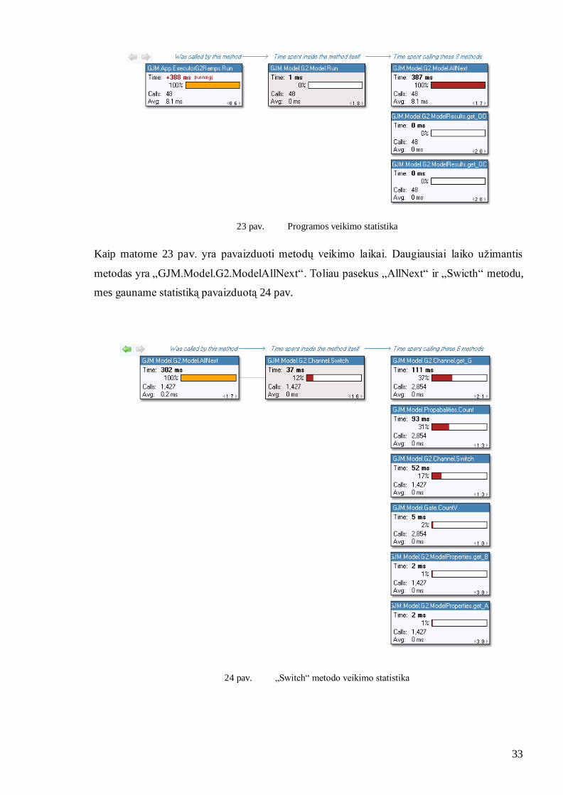
Programinio kodo veikimo charakteristikom perţiūrėti mes pasinaudosime „EQATEC

Profiler“ įrankį, kuris skaičiuoja kviečiamų metodų laikus ir suranda ilgiausiai vykdomą

programinį kodą. Šiam tyrimui atlikti paleisime 2 vartų modelio imitaciją ir surasime

ilgiausiai vykdančius metodus.

33

23 pav. Programos veikimo statistika

Kaip matome 23 pav. yra pavaizduoti metodų veikimo laikai. Daugiausiai laiko uţimantis

metodas yra „GJM.Model.G2.ModelAllNext“. Toliau pasekus „AllNext“ ir „Swicth“ metodu,

mes gauname statistiką pavaizduotą 24 pav.

24 pav. „Switch“ metodo veikimo statistika

34

Taigi kaip matome yra trys daugiausiai laiko vykdantys skaičiavimus metodai, kuriuos reiktų

patikrint ir perţiūrėti ar jie nevykdo nereikalingų arba perteklinių skaičiavimų. Patikrinus

programinį kodą perteklinių skaičiavimų neradome šie metodai vykdė elementarius

matematinius skaičiavimus, todėl galime teigti kad programinis kodas yra parašytas

efektyviai.

Pasinaudodami tokiais įrankiais kaip „EQUATEC Profiler“ mes galime nesunkiai aptikti

blogai veikiantį programinį kodą. Šis įrankis mums padėjo įvertinti programinio kodo

efektyvumą, neskaitant algoritminės pusės.

4.2 SISTEMOS PLĖTOJIMAS

Kadangi yra dar daug nepagrįstų modelių, bei įvairių prielaidų pas uţsakovus bei kitus

tyrinėtojus, šią sistemą ketinama plėtoti bei daryti įvairius pataisymus. Taip pat šiuo metu

paieška yra padaryta tik 2 vartų modeliui, tačiau ji bus įgyvendinta ir kituose modeliuose.

Taip pat yra planuojama leisti naudotis šia sistema visiems vartotojams, ir yra ketinama duoti

prieigą prie jos.

Nors parametrų paieška suranda gana artimus eksperimentų atitikmenis, tačiau jis nėra

pakankamai tikslus, su didesniu triukšmo lygiu tikslumas labai smarkiai sumaţėja. Todėl

parametrų paieškos optimizavimas bus toliau tobulinimas ir bus ieškoma greitesnių

sprendimų, kurie padėtų greičiau aptikti eksperimentinių rezultatų atitikmenis.

Iš anksčiau išvardintų punktų yra aišku, kad sistemos plėtojimo galimybių yra pakankamai

daug, todėl ji toliau yra priţiūrima ir plečiama.

35

5 EKSPERIMENTAI IR IMITACINĖ SISTEMA

Prieš darant eksperimentus noriu pabrėţti, jog čia yra vaizduojami tik pagrindiniai sistemos

išvedami duomenys, kurie parodo bendrą imitacijos, bei eksperimento rezultatą tai yra jos

laidumą. Uţsakovai nagrinėja ir tarpinius duomenis, kurie jiems yra taip pat labai svarbūs.

5.1 EKSPERIMENTŲ IR IMITACIJOS PALYGINIMAS

[1] straipsnyje yra aprašyti eksperimentai įvykdyti su skirtingais koneksonų tipais, todėl

pasinaudoję jų gautais rezultatais mes pabandysime palyginti imitacijos ir eksperimentų

gautus rezultatus. Bet prieš tai noriu pasakyti, kad parametrai nėra tikslūs, ne visi yra ţinomi

ir yra nemaţos paklaidos jose.

25 pav. Imitacijos rezultatai su

Cx30/Cx30 koneksinais

26 pav. Eksperimento rezultatai su

Cx30/Cx30 koneksinais

36

Kaip matome iš. 25 pav. ir 26 pav. šių rezultatų kreivės yra panašios, tačiau nevisai. Tai yra

dėl to kad eksperimento duomenys yra jau sutvarkyti ir normalizuoti, o imitaciniuose

rezultatuose yra atvaizduotas pilnas laidumas, kuris priklauso nuo kanalų skaičiaus. Šioje

imitacijoje naudojome 1000 kanalų su tokiais parametrais:

25.0

;1

;5.41

;116,0

1

1

01

1

Gc

Go

V

A

25.0

;1

;5.41

;116,0

2

2

02

2

Gc

Go

V

A

27 pav. Cx43/Cx45 koneksonų imitacijos

rezultatai

28 pav. Cx43/Cx45 koneksonų

eksperimento rezultatai

27 pav. ir 28 pav. matome Cx43/Cx45 gautus rezultatus. Šis pavyzdys yra tinkamesnis, nes

aiškiau yra matomas kreivių panašumas. Kaip matome rezultatai sutampa. Šiame

eksperimente leidome 1000 kanalų su tokiais parametrais:

04.0

;03.1

;3.22

;088.0

1

1

01

1

Gc

Go

V

A

04.0

;03.1

;3.125

;027.0

1

1

01

2

Gc

Go

V

A

Kaip matome iš šių eksperimentų imitacijos ir eksperimento rezultatai yra panašus. Yra viena

problema atskirų koneksinų parametrai yra labai retai ţinomi ir nelabai tikslūs, todėl ir gavosi

1-as eksperimentas su šiokia tokia paklaida. Literatūros [9] straipsnį yra pateiktas

tarpląstelinių plyšinių jungčių modelio pradinis variantas. Jame matosi jog senesnis modelis

buvo maţiau tikslus nei dabartiniai. Taip pat [10] straipsnį yra demonstruojamas tikslesnis

rezultatų palyginimas ne tik su pagrindiniais duomenim, jame yra parodomi eksperimentų ir

imitacijos palyginimai su lėtais ir greitais vartais.

5.2 GLOBALUS OPTIMIZAVIMAS

Globalaus optimizavimo arba paieškos eksperimentai yra labai svarbūs šiame darbe, todėl

dabar padarysime keletą eksperimentų. Pradţioje pabandysime surasti realių eksperimentų

atitikmenis. Šiam eksperimentui mes iš uţsakovų gavome realius nufiltruotus duomenis, kurie

yra pavaizduoti 29 pav. Plona linija vaizduoja gautus duomenis, o paryškinta vaizduoja

filtravimą pritaikius slenkantį kablelį.

29 pav. Eksperimentiniai duomenys

Šiam eksperimentui naudosime 1000, kanalų tam, kad gautume tikslesnius rezultatus. Taigi

po 3 valandų mes gauname rezultatą pavaizduotą 30 pav. Kaip matome rezultatai yra

pakankamai tikslūs nepaisant esamo triukšmo lygio.

30 pav. Gauti rezultatai po 3 valandų

Dabar pabandysime įvertinti paieškos tikslumą. Kadangi šia tyrimui reikia tikslių duomenų,

tai yra su kuo maţesniu triukšmu, todėl mes naudosime pačios sistemos gautus rezultatus su

1000 kanalų (31 pav.), kurios surasta kreivė po 5000 iteracijų yra pavaizduota32 pav.

G, [pS]

V, [mV]

31 pav. Duomenys gauti panaudojus imitacine sistema

32 pav. Rezultatai gauti po 5000 iteracijų

G, [pS]

V, [mV]

G, [pS]

V, [mV]

33 pav. Maţiausių kvadratų skirtumo priklausomybė nuo iteracijų skaičiaus

Iš 33 pav. galime daryti išvadą, kad kvadratų skirtumas nuo iteracijų skaičiaus maţėja

eksponentiškai link 0, todėl vykdant paiešką yra labai sunku prieiti prie norimo rezultato, ypač

jei yra padidėjęs triukšmo lygis tiek eksperimentuose tiek imitaciniuose rezultatuose.

5.3 ŽMOGIŠKASIS FAKTORIUS

Yra labai daţnas atvejis kai ţmogus gali atlikti kai kuriuos skaičiavimus pasinaudodamas

savo nuojauta. Todėl nusprendţiau patyrinėti kaip greitai ţmogus gali surasti

eksperimentinius duomenis. Kadangi reikia ţmonių, kurie gerai supranta sistemą bei

sprendţiamą problemą, nusprendţiau paimti uţsakovą ir save. 1 Lentelėje surašiau laikus, per

kurį buvo surasti eksperimentinių duomenų atitikmenys pagal 31 pav. pavaizduotą

eksperimentą.

Uţdavinio sprendėjas Laikas

Sistemos programuotojas 35 min.

0

0.2

0.4

0.6

0.8

1

1.2

1.4

1 2 3 4 5 6 7

Iteracijų skaičius 10^3

Kvad

ratų

skir

tum

as

Uţsakovas 20 min.

Kompiuteris 68 min.

1 Lentelė. 31 pav. sprendžiamo uždavinio laikai

Kaip matome suradimo laikas priklauso nuo modelio supratingumo lygio. Tai yra uţsakovas,

kuris daugiausiai naudojasi sistema suranda panašius atitikmenis kaip ir kompiuteris per daug

trumpesnį laiką. Todėl ţmogiškoji nuojauta tokioje sistemoje yra labai svarbi ir ieškant

sudėtingesnių eksperimentų atitikmenis be ţmogaus nesurasime.

Sistemos programuotojas išmano sistema, tačiau negali taip greitai surasti atitikmenų kaip

pats uţsakovas. Todėl galima daryti prielaidą, jog paieška be ţmogaus įsikišimo yra

nereikšminga sprendţiant sudėtingesnius uţdavinius.

Kaip matome tam tikros ţinios gali smarkiai paspartinti paieškos sistemą, nors šiuo metu

paieškos greitis yra pakankamai geras, tačiau likę modeliai yra sudėtingesni ir jų veikimas

uţtrunką 2 ar net 4 kartus ilgiau, todėl paieška bus vykdoma dar ilgiau, todėl yra manoma jog

genetinis arba neuroninis programavimas [8] čia gali padaryti didelę įtaką. Jie gali smarkiai

pagreitinti paieška

6 IŠVADOS

1. Sukurta PJ imitacinė sistema, leidţianti imituoti 2 vartų, 4 vartų ir 6 koneksinų

modelius.

2. Kuriant PJ imitacinius modelius reikia optimaliai parinkti modelio parametrus, kad

modeliavimo rezultatai minimaliai skirtųsi nuo eksperimentų rezultatų. Imitacinio

modelio parametrų parinkimui buvo panaudotos globalaus optimizavimo procedūros.

3. Sukurti PJ modeliai adekvačiai atvaizduoja elektrofiziologinius procesus plyšinėje

jungtyje. Tai patvirtino imitacinio modelio rezultatų palyginimas su eksperimentiniais

rezultatais gautais iš Niujorko, Yeshiva universiteto, Alberto Einšteino koledţo

laboratorijos.

4. Įvertinome programinio kodo efektyvumą pasinaudodami „EQUATIC Profiler“

įrankiu, su kuriuo paskaičiavome programinio kodo vykdymo laikus ir nesunkiai

aptikome ilgiausiai trunkančius metodus, bei įvertinome jų efektyvumą.

5. Įvertinome GJM sistemos plėtojimo galimybes, bei aptarėme ateities planus.

7 LITERATŪRA

1. Ye Chen-Izu, Alonso P. Moreno and Robert A. Spangler. Opposing gates model for

voltage gating of gap junctions channels. Prieiga internete:

http://ajpcell.physiology.org/cgi/content/abstract/281/5/C1604.

2. Feliksas F. Bukauskas, Angelė Bukauskienė, Vytas K. Verselis and Michael V. L

Bennett. Coupling asymmetry of heterotypic connexin 45/ connexin 43-EGFP gap

junctions: Properties of fast and slow gating mechanisms. Prieiga internete:

http://www.ionchannels.org/showabstract.php?pmid=12011467.

3. Mindaugas Račkauskas, Maria M. Kreuzberg, Mindaugas Pranevičius, Klaus

Willecke, Vytas K. Verselis and Feliksas Bukauskas. Gating properties of Heterotypic

Gap Junction Channels Formed of connexin 40, 43 and 45. Biophysical Journal, 2007.

4. Computer simulation. Prieiga internete:

http://en.wikipedia.org/wiki/Computer_simulation.

5. Globalaus optimizavimo pavyzdţiai. Prieiga internete: http://soften.ktu.lt/~mockus/.

6. Nonlinear estimation. Prieiga internete:

http://www.statsoft.com/textbook/stnonlin.html

7. H. Pranevičius. Kompiuterinių tinklų formalusis specifikavimas: agregatinis metodas.

Kaunas. Technologija, 2003, 2004.

8. A. Verikas, A. Gelţinis. Neuroniniai tinklai ir neuroniniai skaičiavimai. Kaunas.

Technologija, 2003.

9. Mindaugas Pranevičius, Feliksas Bukauskas, Henrikas Pranevičius ir Nerijus

Paulauskas. Imitacinis tarpląstelinių plyšinių jungčių vartų modeliavimas.

Informacinės technologijos, Kaunas, 2007.

10. Nerijus Paulauskas, Mindaugas Pranevičius, Henrikas Pranevičius, and Feliksas F.

Bukauskas. A Stochastic Four-State Model of Contingent Gating of Gap Junction

Channels Containing Two „„Fast‟‟ Gates Sensitive to Transjunctional Voltage.

Biophysical Journal, 2009.

http://ajpcell.physiology.org/cgi/content/abstract/281/5/C1604

http://www.ionchannels.org/showabstract.php?pmid=12011467

http://en.wikipedia.org/wiki/Computer_simulation

http://soften.ktu.lt/~mockus/

http://www.statsoft.com/textbook/stnonlin.html

8 TERMINŲ IR SANTRUMPŲ ŢODYNAS

GJM – formalus imitacinės sistemos pavadinimas (Gap Junction Model).

PJ – plyšinės jungtys.

Cx – Koneksinai, daţnai rašomi su numeriu priekyje nusakančiu jo rūšį pvz.: Cx30, Cx32.

Protokolas – aprašo įtampos kitimą, kuri kiekvienu laiko momentu paduodama kanalui.

9 PRIEDAS

1. Nerijus Paulauskas, Mindaugas Pranevičius, Henrikas Pranevičius, and Feliksas F.

Bukauskas. A Stochastic Four-State Model of Contingent Gating of Gap Junction

Channels Containing Two „„Fast‟‟ Gates Sensitive to Transjunctional Voltage.

Biophysical Journal, 2009.

2. Mindaugas Pranevičius, Feliksas Bukauskas, Henrikas Pranevičius ir Nerijus

Paulauskas. Imitacinis tarpląstelinių plyšinių jungčių vartų modeliavimas.

Informacinės technologijos, Kaunas, 2007.

3936 Biophysical Journal Volume 96 May 2009 3936–3948

A Stochastic Four-State Model of Contingent Gating of Gap Junction Channels Containing Two ‘‘Fast’’ Gates Sensitive to Transjunctional Voltage

Nerijus Paulauskas,†§ Mindaugas Pranevicius,ffi Henrikas Pranevicius,§ and Feliksas F. Bukauskas†* Dominick P. Purpura Department of Neuroscience, and ffiAnesthesiology, Albert Einstein College of Medicine, The Bronx, New York; and §Kaunas University of Technology, Kaunas, Lithuania †

ABSTRACT Connexins, a family of membrane proteins, form gap junction (GJ) channels that provide a direct pathway for elec - trical and metabolic signaling between cells. We developed a stochastic four-state model describing gating properties of homotypic and heterotypic GJ channels each composed of two hemichannels (connexons). GJ channel contain two ‘‘fast’’ gates (one per hemichannel) oriented opposite in respect to applied transjunctional voltage (V j). The model uses a formal scheme of peace-linear aggregate and accounts for voltage distribution inside the pore of the channel depending on the state, unitary conductances and gating properties of each hemichannel. We assume that each hemichannel can be in the open state with conductance gh,o and in the residual state with conductance gh,re s, and that both gh,o and gh,re s rectifies. Gates can exhibit the same or different gating polarities. Gating of each hemichannel is determined by the fraction of Vj that falls across the hemichannel, and takes into account contingent gating when gating of one hemichannel depends on the state of apposed hemichannel. At the single-channel level, the model revealed the relationship between unitary conductances of hemichannels and GJ channels and how this relationship is affected by gh,o and gh,res rectification. Simulation of junctions containing up to several thousands of homotypic or heterotyp ic GJs has been used to reproduce experimentally measured macroscopic junctional current and Vj-dependent gating of GJs formed from different connexin isoforms. Vj-gating was simulated by imitating several frequently used experimental protocols: 1), consecutive Vj steps rising in amplitude, 2), slowly rising Vj ramps, and 3), series of Vj steps of high frequency. The model was used to predict Vj-gating of heterotypic GJs from characteristics of corresponding homotypic channels. The model allowed us to identify the parameters of Vj-gates under which small changes in the difference of holding potentials between cells forming heterotypic junctions effectively modulates cell-to-cell signaling from bidirectional to unidirectional. The proposed model can also be used to simulate gating properties of unapposed hemichannels.

INTRODUCTION

Connexins (Cxs), a large family of membrane proteins, form gap junction (GJ) channels that provide a direct pathway for electrical and metabolic signaling between cells. Each GJ channel is composed of two hemichannels, hexamers of Cxs also called connexons. Cell-cell communication can be orga- nized through homotypic (same Cx isoform in both hemichannels), heterotypic (two Cx isoforms form GJ channels, but each hemichannel is assembled from one isoform) and heteromeric (different Cx isoforms form at least one hemichannel) GJ channels that vary in conductance, perm-selectivity, and gating properties. Gap junctional communication play important roles in many processes, such as impulse propagation in the heart, communication between neurons and glia, metabolic exchange between cells in the lens that lack blood system, organ formation during development, and regulation of cells proliferation (reviewed in (1–4)). A property that appears to be common to GJ channels formed of any Cx isoform is sensitivity of junctional conductance, gj, to transjunctional voltage, Vj (5,6). A common

feature of Vj-gating is that steady-state gj (gss) does not decline to zero with increasing Vj, but reaches a plateau or residual conductance that varies from ~5% to 30% of the maximum gj depending on the Cx isoforms (7). Single-channel studies have shown that residual gj is due at least in part to incomplete closure of the GJ channel by Vj, i.e., Vj causes channels to close to a subconductance (residual) state with fast gating transitions (~1 ms and less), which has significantly longer dwelling time than other substates (7,8). The symmetric reduction in gj with positive or negative Vj has been explained by having a Vj gate in each apposed hemichannel so that for each polarity of Vj, closure can be ascribed to one or the other hemichannel (9). It was shown that Vj as well as chemical uncouplers can also induce gating transitions to the fully closed state and that these transitions are slow, ~10 ms (10,11). Gating to different levels via distinct fast and slow gating transitions led to the suggestion that there are two distinct Vj sensitive gates, termed fast and slow or ‘‘loop’’ gating mechanisms (reviewed in (12)). The fast gate closes channels to the residual state and it is mainly operated by Vj, whereas the slow gate closes channels completely and it is operated primarily by chemical uncouplers but also by Vj. Earlier, gating properties of GJ channels were described by using Boltzmann function (9,13) assuming that GJ channels have two states, open and fully closed, as most of ionic

Submitted August 25, 2008, and accepted for publication January 14, 2009. Nerijus Paulauskas and Mindaugas Pranevicius contributed equally to this work.

*Correspondence: [email protected] Editor: Benoit Roux. Ó 2009 by the Biophysical Society 0006-3495/09/05/3936/13 $2.00

doi: 10.1016/j.bpj.2009.01.059

Modeling of Gap Junction Channels Gating 3937

2; HEPES, 5 (pH 7.4). Electrodes were filled with pipette solution containing (in mM): KCl, 130; NaAsp, 10; MgATP, 3; MgCl2, 1; CaCl2, 0.2; EGTA, 2; HEPES, 5 (pH ¼ 7.2). For electrophysiological recordings, cells were grown onto glass coverslips and transferred to an experimental chamber mounted on the stage of an inverted microscope IX70 (Olympus, Center Valley, PA). Cells were perfused with modified Krebs-Ringer solution at room tempera- ture. Junctional conductance (gj) was measured in selected cell pairs using the dual whole-cell patch clamp system (20). Briefly, each cell within a pair was voltage clamped independently with a separate patch clamp amplifier (EPC-7plus; HEKA). Transjunctional voltage (Vj) was induced by stepping the voltage in cell-1 (DV1) and keeping the other constant, Vj ¼ DV1. Junc- tional current (Ij) was measured as the change in current in the unstepped cell-2, Ij ¼ DI2. Thus, gj was obtained from the ratio, ÀIj/Vj, where negative sign indicates that junctional current measured in cell-2 is oppositely oriented to the one measured in cell-1. Signals were acquired and analyzed using custom-made software (21) and A/D converter from National Instruments (Austin, TX).

channels. To find gating parameters, gj-Vj dependence was split into two segments for positive and negative Vjs. Such approach allowed to describe gating properties of homotypic and heterotypic GJ channels assuming that each hemichannel gates independently, which may be accurate only when both hemichannels have the same gating polarity, have similar single-channel conductance, and are relatively insensitive to Vj. Previously there were few attempts to describe Vj gating of GJs at the single-channel level (14) and macro- scopically (15) by using a four-state model in which each hemichannel contained a fast gate operating between open and residual states. Both models made a progress introducing a more detailed description of GJ channels based on most recent experimental data and improved the fitting process allowing to find gating parameters of GJ channels. However, the analytical approach used in (15) to describe Vj-gating allowed only steady-state predictions. Neither of the previous models allowed the possibility to study kinetics of junctional current during applied transjunctional voltages. Ramanan et al. (16) proposed a three-state model of Cx37 GJ channels that exhibits the main state and two substates. This model was adapted more specifically to GJ channels that demonstrate multiple substates. Here we present a stochastic four-state model that uses imitative approach and accounts for voltage distribution inside the pore of the GJ channel, i.e., takes into account contingent gating. Each hemichannel contains a fast gating mechanism with variable gating polarity. Each gate can be in open or closed states that correspond to the open state or the residual state, respectively, of the hemichannel. In addition, unitary conductances of open and residual states depend on Vj, i.e., conductance of hemichannels rectifies. The model was used to imitate experimental data of Vj-gating in homotypic and heterotypic junctions measured in HeLa cells exogenously expressing different Cx isoforms. Our model allowed simulation of the dynamics of junctional current that was achieved due to use of stochastic description of voltage gating processes. This enhanced flexibility of the model in respect to its structure and variation of parameters used to describe the conductance and gating of hemichannels composing GJ channel.

MATERIAL AND METHODS

Cells and culture conditions

Experiments were performed using HeLa cells (Human cervix carcinoma cells, ATCC CCL2) stably transfected with different Cx isoforms (Cx31, Cx40, Cx43, Cx45, and Cx47). More details about used DNAs for transfec- tion and selection of clones stably expressing different Cx isoforms are in (17–19). Cells were grown in Dulbecco’s modified Eagle’s medium supple- mented with 8% fetal calf serum (Gibco, Carlsbad, CA), 100 mg/ml strepto- mycin and 100 units/ml penicillin.

RESULTS

Initially, we will highlight the experimental data demonstrating basic properties of GJs that we used in the model. This includes micro- and macroscopic Vj-gating events, single GJ channel gating transitions between open and residual states, and their rectification. Subsequently, we will describe the model and simulate Vj-gating in homo- and heterotypic junctions composed of different numbers of GJ channels. Finally, we will simulate signal transfer asymmetry in response to electrical activity of high frequency applied to either side of heterotypic junctions.

Conductance and voltage gating properties of GJ channels formed from different Cx isoforms

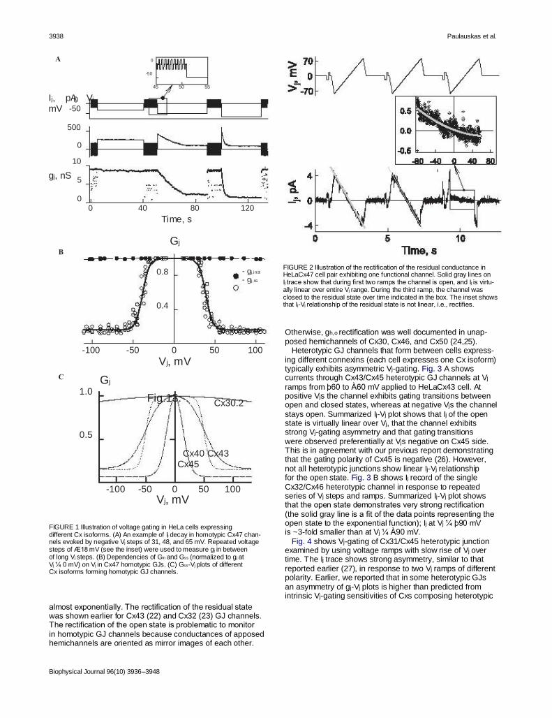
Typically, homotypic GJ channels exhibit gj decay in response to Vj and symmetric gss-Vj dependence. Fig. 1 A shows Ij through Cx47 homotypic channels evoked by negative Vj steps of 31, 48, and 65 mV. Short and repeated voltage steps of Æ18 mV (see the inset) were used to measure gj in between of long Vj steps. During Vj steps of À48 and À65 mV, Ij decayed from an initial value (Iin) to a steady-state level (Iss). Fig. 1 B shows averaged and normalized Gin and Gss (normalized to gj at Vj ¼ 0 mV) dependencies on Vj. Gin-Vj plot (solid circles; dashed line is a regression line of the second order) shows virtually no changes of Gin over Vj range from À110 to 110 mV. Gss- Vj plot demonstrates symmetric bell-shape dependence on Vj that is typical for homotypic GJ channels. The solid line is a fit of Gss data to Boltzmann’s equation (13). The fit was performed separately for gss data at positive and negative Vjs. Fig. 1 C shows variation of Gss-Vj dependence among different Cx isoforms forming homotypic GJ channels. Fig. 2 shows Ij record of HeLaCx47 cell pair exhibiting one functional channel. Solid gray lines show that during first two ramps, the channel is open and Ij is virtually linear over applied Vjs. At the beginning of the third ramp, channel closes from the open state to the substate or the residual state and remains closed during period indicated in the box. The inset shows that Ij-Vj relationship is not linear and rectifies

Biophysical Journal 96(10) 3936–3948

Electrophysiological measurements

Experiments were performed in modified Krebs-Ringer solution containing (in mM): NaCl, 140; KCl, 4; CaCl2, 2; MgCl2, 1; glucose, 5; pyruvate,

3938 Paulauskas et al.

A 0

-50

45 50 55 Ij, pA Vj, mV

gj, nS

0 -50

500

0

10

5

0 0 40 80 120

Time, s

B Gj

0.8

0.4

- gj ,inst - gj ,ss

FIGURE 2 Illustration of the rectification of the residual conductance in HeLaCx47 cell pair exhibiting one functional channel. Solid gray lines on Ij trace show that during first two ramps the channel is open, and Ij is virtually linear over entire Vj range. During the third ramp, the channel was closed to the residual state over time indicated in the box. The inset shows that Ij-Vj relationship of the residual state is not linear, i.e., rectifies.

-100

C

-50 Vj, mV

0 50 100

1.0 Gj

Fig.13. Cx30.2

0.5

Cx40 Cx43 Cx45

-100 -50 Vj, mV

0 50 100

FIGURE 1 Illustration of voltage gating in HeLa cells expressing different Cx isoforms. (A) An example of Ij decay in homotypic Cx47 channels evoked by negative Vj steps of 31, 48, and 65 mV. Repeated voltage steps of Æ18 mV (see the inset) were used to measure gj in between of long Vj steps. (B) Dependencies of Gin and Gss (normalized to gj at Vj ¼ 0 mV) on Vj in Cx47 homotypic GJs. (C) Gss-Vj plots of different Cx isoforms forming homotypic GJ channels.

almost exponentially. The rectification of the residual state was shown earlier for Cx43 (22) and Cx32 (23) GJ channels. The rectification of the open state is problematic to monitor in homotypic GJ channels because conductances of apposed hemichannels are oriented as mirror images of each other.


Otherwise, gh,o rectification was well documented in unapposed hemichannels of Cx30, Cx46, and Cx50 (24,25). Heterotypic GJ channels that form between cells expressing different connexins (each cell expresses one Cx isoform) typically exhibits asymmetric Vj-gating. Fig. 3 A shows currents through Cx43/Cx45 heterotypic GJ channels at Vj ramps from þ60 to À60 mV applied to HeLaCx43 cell. At positive Vjs the channel exhibits gating transitions between open and closed states, whereas at negative Vjs the channel stays open. Summarized Ij-Vj plot shows that Ij of the open state is virtually linear over Vj, that the channel exhibits strong Vj-gating asymmetry and that gating transitions were observed preferentially at Vjs negative on Cx45 side. This is in agreement with our previous report demonstrating that the gating polarity of Cx45 is negative (26). However, not all heterotypic junctions show linear Ij-Vj relationship for the open state. Fig. 3 B shows Ij record of the single Cx32/Cx46 heterotypic channel in response to repeated series of Vj steps and ramps. Summarized Ij-Vj plot shows that the open state demonstrates very strong rectification (the solid gray line is a fit of the data points representing the open state to the exponential function); Ij at Vj ¼ þ90 mV is ~3-fold smaller than at Vj ¼ À90 mV. Fig. 4 shows Vj-gating of Cx31/Cx45 heterotypic junction examined by using voltage ramps with slow rise of Vj over time. The Ij trace shows strong asymmetry, similar to that reported earlier (27), in response to two Vj ramps of different polarity. Earlier, we reported that in some heterotypic GJs an asymmetry of gj-Vj plots is higher than predicted from intrinsic Vj-gating sensitivities of Cxs composing heterotypic


A

B

FIGURE 4 Vj-gating in HeLa cell pair forming Cx31-EGFP/Cx45 heterotypic junctions. Ij trace shows strong asymmetry of Ij response to Vj ramps slowly rising from 0 to À115 mV and from 0 to 115 mV. Gj-Vj plot (normalized to maximal gj at Vj ¼ ~À40 mV) shows that at Vj ¼ 0 only ~50% of Cx31-EGFP/Cx45 channels are open. Data shown in the inset demonstrate an increase of gj at Vjs >60 mV.

FIGURE 3 Ij recordings at the single-channel level demonstrating an absence and presence of Ij-Vj rectification of the open state in Cx43/Cx45 (A) and Cx32/Cx46 (B) heterotypic junctions, respectively.

GJ channels (26,27). We hypothesized that a difference in unitary conductances of hemichannels affects asymmetry of gj-Vj plot. We will exploit the model by using voltage ramp protocol to study Vj-gating to validate this statement (see Fig. 10).

The gss-Vj plot calculated from Vj and Ij traces allows us to suggest that at Vj ¼ 0 only a fraction (<1/2) of Cx31/Cx45 channels are open and gss increases when the Cx45 side is relatively more positive and decreases almost to zero when the Cx45 side is more negative. Similar gj-Vj gating asymmetry was documented in other heterotypic junctions, such as Cx43/Cx45 (26) and Cx40/Cx45 (20). Interestingly, the data shown in the inset demonstrate that when Vj increased from 60 to 110 mV, gss increased. This phenomenon was reproduced in the model by assuming a presence of conductance rectification of the residual state of Cx45 (see Fig. 9 E). In summary, heterotypic GJs in contrast to homotypic GJs demonstrate asymmetric Vj-gating. Vj-gating of GJ channel depends on intrinsic gating properties of composing hemichannels as well as on the fraction of Vj that drops on each of them. This fraction is 1/2 for open homotypic GJ channels, and it can be very different for heterotypic GJ channels formed from Cxs that demonstrate different unitary conductances. In addition, data shown in Figs. 2 B and 3 B demonstrate that Ij-Vj relationship of the single channel of open and residual states can rectify. Thus, in the model, we should take



into account Cx-type dependent Vj-gating sensitivity, unitary conductances of open and residual states, as well as their I/V rectification.

Description of the model

Schematics of transitions between states

In the model, we assume that the GJ channel is formed from A and B hemichannels, and each hemichannel contributes one voltage-sensitive gate that closes channels to the residual state, i.e., imitates the fast gating mechanism (12). Therefore, in concert with previous models (13–15), we assume that two voltage gates in series control the gating of GJ channel (Fig. 5 A). The schematic presentation of the four-state model is shown in Fig. 5 B, where Ki (i ¼ 1, 2, 3, 4) are equilibrium constants for each of transitions between states. The channel can occupy one of the four possible states: 1), AoBo, both gates are open, 2), AcBo, A gate is closed and gate B is open, 3), AoBc, A gate is open and B gate is closed, and 4), AcBc, both gates are closed. The equilibrium constants between the states were described as exponential functions that depend on transjunctional voltage across the hemichannels A and B (VA and VB; we assume that transjunctional voltage across the gate and hemichannel is the same):

K1 K2 K3 K4

¼ ¼ ¼ ¼

e A1 ðÀP , VA ÀV01 Þ e A2 ðP , VB ÀV02 Þ ; e A3 ðÀP , VA ÀV03 Þ e A4 ðP , VB ÀV04 Þ

(1)

where Ai is the voltage sensitivity coefficient; Voi is the voltage for half-maximal conductance; and P is a gating polarity, which can be positive or negative. Negative and positive signs for VA and VB, respectively, indicate that the two gates are oriented as mirror images of each other. Trans- junctional voltage across the GJ channel is a sum of VA and VB, i.e., Vj ¼ VA þ VB. Closing one hemichannel changes the voltage across the apposing hemichannel, and this will affect

the probability of changing the state. Thus, the model exploits principles of contingent gating. Aggregate method was used for a formal description of the model and conse- quently for writing the algorithm (see Supplement 2 in the Supporting Material). The piece-linear aggregate is described in accordance with Markov principles, i.e., the probability of transitions does not depend on the history of previous transitions. The algorithm was written using C Sharp (C#) programming language. Assuming that both gates do not interact with each other except via voltage redistribution inside the pore and only voltage across each of A and B hemichannels defines their gating, then A1 ¼ A3, A2 ¼ A4, V01 ¼ V03, and V02 ¼ V04. As reported earlier (15), regardless of the pathway of transitions between states AoBo and AcBc, thermodynamic law requires that K1 Â K4 ¼ K2 Â K3. Following the scheme shown in Fig. 5 B, opening and closing probabilities of gate A depend on K1: P(Ao/c) ¼ K1 Â P(Ac/o). We will define such a small time interval, Dt, at which only one transition for each gate is possible. Interval Dt will be used as a simulation step. For example, when K1 ¼ 1, both open and closed states of the gate are equally possible, P(Ao) ¼ P(Ac). When system is at equilibrium, average number of open and closed gates does not change. Thus, the average number of opening and closing events of the gate must be equal or PðAo Þ Â PðAo/c Þ ¼ PðAc Þ Â PðAc/o Þ. If we label Pk as a probability that the gate will change the state during time interval Dt, then Pk ¼ PðAo Þ Â PðAo/c Þ þ PðAc ÞÂ PðAc/o Þ. When both states are equally probable (K1 ¼ 1), then P(Ao) ¼ P(Ac) ¼ 1/2 and Pk ¼ (P(Ao/c) þ P(Ac/o))/2. The difference, 1 À Pk, is a probability that the gate will stay in the same state. In general, the model defines at any given time whether individual channels remain in the same state or change the state. In junction composed of thousands of GJ channels any new calculation at the same Vj protocol results to random distribution of open and closed states over time for individual channels while the mean gj remains the same.

Conductance of hemichannels

A B

FIGURE 5 Schematics of the four-state model. (A) The scheme of the GJ channel containing the fast gate in each hemichannel. (B) Illustration of a four-state model: 1), AoBo—both gates are open, 2), AcBo—gate A closed and gate B open, 3), AoBc—gate A open and gate B closed, and 4), AcBc—both gates closed. Ki (I ¼ 1–4) are equilibrium constants.


The proposed model assumes that each hemichannel can be in the open or the closed states with conductances, gh,o and gh,res, respectively. Studies of the single GJ channel formed of various Cx isoforms show that the ratio of gres/go is in the range of 0.2–0.25. The ratio, gh,res/gh,o, for hemichannels should be different and for homotypic GJs gres/go ¼ 2(gh,res/ gh,o)/(1þgh,res/gh,o). However, this relationship could be more complex if both gh,o and gh,res depend on Vj, i.e., when they demonstrate rectifying properties as it is shown in Figs. 2 B and 3 B. Similar to (14), we used single exponential function to describe gh,o and gh,res dependence on Vj: gh,o ¼ ^^Goe(ÀVj/6o) and gh,res ¼ Grese(ÀVj/6res), where Go and Gres are unitary conductances of hemichannels at Vj ¼ 0 mV, and 6o and 6res determine rectification constant. We generated three versions of the model that differ in stimulation protocols: 1), consecutive Vj steps rising in the


amplitude, 2), slowly raising Vj ramps, and 3), series of short negative and positive Vj steps of variable frequency. In Supplement 1 in the Supporting Material, we show examples of the screen captures for each of used protocols (see Fig. S1, Fig. S2, and Fig. S3).

Simulation of homotypic GJ channels

Single-channel gating

Fig. 6 A shows Ij recordings in response to three consecutive Vj steps of À20, À60, and À100 mV. We assumed that the cell

A

B

pair forms single homotypic GJ channel with parameters identical for both hemichannels: Vh,o ¼ 40 mV gh,o ¼ 200 pS, gh,res ¼ 25 pS, Ah ¼ 0.05 mVÀ1 (Vh,o corresponds to Voi, and Ah corresponds to AA or AB in Eq. 1; in homotypic GJ channel AA ¼ AB and Vo,A ¼ Vo,B). In addition, it was assumed that both open and residual states do not rectify, i.e., 6o ¼ N and 6res ¼ N. Ij traces show that open channel probability decays with Vj increase, and three conductance states can be distinguished, which are best seen in Ij trace at Vj ¼ 100 mV. When the channel is fully open, Ij ¼ 10 pA. When one hemichannel is closed to the residual state (Ij ¼ 2.2 pA), we call this state as a primary residual state. The arrow shows the substate that we call the secondary residual state when two gates are closed (Ij ¼ 1.3 pA). An overlay of gj traces for all three voltage steps show that go¼100 pS, whereas gres is equal 22 pS for the primary residual state and 13 pS for the secondary residual state. When the ratio gh,res/gh,o ¼ 0.125 (25 pS/200 pS) then for the primary residual state gres/go ¼ 0.222 (22.2 pS/100 pS). Experimental data show that for different connexins gres/go is in between 0.2 and 0.25 (12). According to the model, to cover this range of gres/go, the ratio, gh,res/gh,o, should be in the range of 0.111–0.143, i.e., ~2-fold smaller. Fig. 6 B shows an example of Ij trace of the single channel at Vj ¼ 60 mV. All parameters are the same as in Fig. 6 A but the open and residual states exhibit I/V rectification with 6o ¼ 400 mV and 6res ¼ 200 mV. gj trace obtained superposing gjs at three Vjs, as in Fig. 6 A, demonstrates that both go is gres are not constant. Next to gj trace, we show the frequency histogram, which demonstrates that at these particular Vjs three states can be distinguished for go and nine states for gres. Repeated simulations, which results in stochastic data sets, show that we are getting 96, 98, and 99 pS for go and more substate conductances in the range of 9–25 pS. There- fore, I/V rectification can result to a large variety of go and gres measured experimentally at different Vjs. In summary, for homotypic nonrectifying GJ channel, we can expect having one conductance for go and two conductances for gres. The ratio, gh,o/gh,res, for hemichannels is approximately twice smaller than ratio, go/gres, for GJ channel. If hemichannels exhibit I/V rectification of open and residual states, then in GJ channel both go and gres depend on applied Vjs, but gres varies in broader range than go.

Vj-gating of homotypic junctions

FIGURE 6 Simulation of the junction containing single homotypic GJ channel. The following parameters were identical for both hemichannels: Vh,o ¼ 40 mV, gh,o ¼ 200 pS, gh,res ¼ 25 pS, and Ah ¼ 0.05 mVÀ1. (A) Ij and gj traces of nonrectifying channel simulated at three Vj steps of À20, À60, and À100 mV. gj trace is an overlay of conductances calculated for all three voltage steps. (B) Ij and gj traces of the channel exhibiting gh,o and gh,res rectification with 6 o¼ 400 mV and 6res ¼ 200 mV. Ij trace shows single channels gating at Vj ¼ À60 mV. The bottom gj trace shows overlay of conductances at Vj steps of À20, À60, and À100 mV.

Fig. 7 shows theoretically predicted Gj (normalized to gj at Vj ¼ 0) dependences on Vj. In these calculations, we used identical set of parameters for both hemichannels (gh,o ¼ 200 pS, gh,res ¼ 25 pS, Vh,o ¼ 40 mV Ah ¼ 0.1 mVÀ1, 6o ¼ N and 6res ¼ N) and for each plot only one parameter of six varied. For a clearer description, the hemichannels forming GJ channels were attributed to the left- and right-side hemichannels. In all plots, the same color represents different measured parameters: 1), black lines for Gin; 2), gray lines for Gss; 3), blue and red lines for the right-side and the left-side hemichannels,



A B

C D

E F

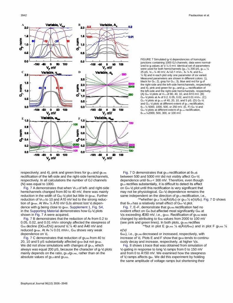
FIGURE 7 Simulated gj-Vj dependencies of homotypic junctions containing 1000 GJ channels; data were normalized to gj values at Vj ¼ 0 mV. Identical set of parameters were used for both hemichannels (gh,o ¼ 200 pS, gh,res ¼ 25 pS, Vh,o ¼ 40 mV, Ah¼0.1 mVÀ1, 6o ¼ N, and 6res ¼ N) and in each plot only one parameter of six varied. Measured parameters are shown in different colors: 1), black for Gin; 2), gray for Gss; 3), blue and red for gj of the right-side and the left-side hemichannels, respectively; and 4), pink and green for gh,o and gh,res rectification of the left-side and the right-side hemichannels, respectively. (A) Gss-Vj plots at Vh,o of 80, 40, 10, and À10 mV. (B) Gss-Vj plots at Ah of 0.2, 0.05, 0.02, and 0.01 mVÀ1. (C) Gss-Vj plots at gh,res of 40, 20, 10, and 5 pS. (D) Gin-Vj and Gss-Vj plots at different extent of gh,o rectification, 6h,o ¼ 5000, 1000, 500, or 250 mV. (E, F) Gin-Vj and Gss-Vj plots at different extent of gh,res rectification, 6h,res¼2000, 500, 300, or 100 mV.

respectively; and 4), pink and green lines for gh,o and gh,res rectification of the left-side and the right-side hemichannels, respectively. In all calculations the number of GJ channels (N) was equal to 1000. Fig. 7 A demonstrates that when Vh,o of left- and right-side hemichannels changed from 80 to 40 mV, there was mainly reduction in the width of Gss-Vj plot but little in gmax. Further reduction of Vh,o to 10 and À10 mV led to the strong reduction of gmax. At Who ¼ À10 mV GJs almost lost Vj dependence with gj being close to gmin. Supplement 1, Fig. S4, in the Supporting Material demonstrates how Gj-Vj plots shown in Fig. 7 A were acquired. Fig. 7 B demonstrates that the reduction of Ah from 0.2 to 0.05, 0.02, and 0.01 mVÀ1 strongly affected the steepness of Gss decline (DGss/DVj) around Vj ¼ 40 and À40 mV and reduced gmax. At Ah ¼ 0.01 mVÀ1, Gss shows very weak dependence on Vj. Fig. 7 C demonstrates that reduction of gh,res from 40 to 20, 10 and 5 pS substantially affected gmin but not gmax. We did not show simulations with changes of gh,o, which always was equal 200 pS, because the character of gj-Vj plots mainly depends on the ratio, gh,o/gh,res, rather than on the absolute values of gh,o and gh,res.


Fig. 7 D demonstrates that gh,o rectification at 6h,os between 500 and 5000 mV did not visibly affect Gin-Vj dependence until 6h,o < 300 mV. Therefore, even though gh,o rectifies substantially, it is difficult to detect its effect on Gin-Vj plot until this rectification is very significant that may not be physiological. Gin-Vj dependence remains the same independent on the direction of gh,o rectification, i.e., ^̂ whether gh,o ¼ e(ÀVj/6o) or gh,o ¼ e(Vj/6o). Fig. 7 D shows that 6h,o has a relatively small effect of Gss-Vj plot. Fig. 7, E–F, demonstrate that gh,res rectification had no evident effect on Gin but affected most significantly Gss at Vjs exceeding Æ80 mV, i.e., gmin. Rectification of gh,res was changed by attributing to 6res values from 2000 to 100 mV (see pink and green lines). In both plots, gh,res rectifies ^^but in plot E gh,res ¼ e(ÀVj/6res) and in plot F gh,res ¼ e(Vj/ 6res), i.e., gh,res decreased or increased, respectively, with increase of Vj. Plots E and F show that gmin tends to continu- ously decay and increase, respectively, at higher Vjs. Fig. 8 shows Ij trace that was obtained from simulation of Vj-gating in response to long Vj ramps from 0 to 150 mV and from 0 to À150 mV. We examined how the steepness of Vj ramps affects gss. We did this experiment by holding the same amplitude of voltage ramps but shortening their


Vj-gating of heterotypic junctions

FIGURE 8 Simulation of Vj-gating in homotypic GJs in response to slowly rising Vj ramps from 0 to þ150 and from 0 to À150 mV. The slope of ramps was changed by shortening their duration from 200 to 100, 40, 20, and 10 s.

duration stepwise from 200 to 100, 40, 20, and 10 s. At dura- tions of Vj ramps longer than 200 s, gss-Vj plots practically overlapped (not shown) and were identical to that measured by applying consecutive Vj steps of ~30 s or longer. When Vj steps are used, it is possible to visualize whether steps are long enough (Tmin) to reach the steady state that is not so obvious with the use of Vj ramps. At Vj ramps shorter than 100 s, gss-Vj plots become broader suggesting that steady state of gj was not yet reached. Our data show that to reach the steady state, the duration of Vj ramps should be several times longer than Tmin used for Vj steps. In experimental studies, it is preferable to use slowly raising voltage ramps instead of consecutive Vj steps because it requires less time to measure gss-Vj plot and it is continuous over entire Vj range. Thus, the model can be used to predict an optimal length of Vj ramps for Vj-gating studies in cells expressing different Cx isoforms. In summary, data shown in Figs. 7 and 8 demonstrate the influence that each of the independent parameters has on the gating properties of homotypic GJ channels. Shown data demonstrate a consistency independently whether consecutive Vj steps or slow Vj ramps were used to study Vj-gating properties of GJ channels.

Fig. 9 shows the gj-Vj plot of a heterotypic junction. In this simulation, we used two sets of parameters (see Fig. 9 A) that are close to those of Cx43 (cell-1) and Cx45 (cell-2). Of all heterotypic junctions, the Vj-gating properties of Cx43/Cx45 junctions are among the most examined (28,26). Fig. 9 B shows the protocol used to simulate gj-Vj dependence. Ij was calculated in response to consecutive Vj steps increasing stepwise (DVj ¼ 20 mV) from À100 to 100 mV. gj trace shows that during time period from 0 to 30 s (Vj ¼ 0 mV) gj decayed from ~50 nS reaching the steady state at 39 nS. This decay is caused by the fact that at the starting point we always assumed that GJ channels are fully open and time window of ~10–30 s was used to allow the system to reach the steady state before Vj protocol was applied. gss-Vj plot (Fig. 9 C; gray line) calculated with the parameters shown in panel A demonstrates a strong Vj-gating asymmetry. The family of gss-Vj plots show that an asymmetry of Vj-gating increased with the reduction of Vh,o of Cx45 from 30 to 10, À10, À30, and À50 mV. We observed similar changes in Cx43/Cx45 GJs during acidification of the cyto- plasm (F. F. Bukauskas, unpublished data). To assess an effect of conductance rectification on Vj-gating, we varied 6o and 6res, whereas other parameters remained the same as shown in Fig. 9 A. Fig. 9 D demonstrates that reduction of 6o from 5000 (circles) to 500 (diamonds) and 250 mV (triangles) has small effect on gss-Vj dependence (gray lines) but increased steepness of gin-Vj plots (black lines). Interestingly, similar changes of 6o did not affect substantially gin of homotypic junctions (see Fig. 7 D). There- fore, an effect of gh,o rectification on gin is obscured in homotypic junctions and is more expressed in heterotypic junctions. Fig. 9 E demonstrate that reduction of 6res from 4000 (circles) to 400 (diamonds) and 200 mV (triangles) did not affect gin-Vj dependence (black lines) but modified gss-Vj plots (gray lines) at higher Vjs. The inset in Fig. 9 E highlights gss increase with increase of Vj. We observed similar phenomena in Cx45/Cx31 (27), Cx45/Cx40 (20), and Cx45/Cx43 (26) junctions (see also the inset in Fig. 4). Therefore, the model allows us to suggest that this gss increase may be caused, at least in part, by gh,res rectification. Previously, Vj-gating asymmetry was commonly used to determine the gating polarity of Cxs composing heterotypic junctions (29,30). This practice was based on an assumption that Vj-gating of heterotypic junctions at different Vj polarities reflects intrinsic gating properties of composing hemichannels. We tested this by superposing simulated gss-Vj plot of heterotypic junction with those corresponding to homotypic junctions. Gray lines in Fig. 10 A show gss-Vj plots of Cx43 and Cx45 homotypic junctions with parameters shown in Fig. 9 A. Solid black line 1 shows gss-Vj plot of heterotypic junction with parameters used for simulation of corresponding homotypic junctions. To examine how the difference in unitary conductances of composing hemichannels affect



A

B

Cell-1 (Cx43): h,o =220 pS h,res =25 pS Ah =0.1 Vh,o=40 mV

Cell-2 (Cx45): h,o =65 pS h,res=2 pS Ah =0.1 Vh,o=10 mV

Cell-1

A

Vj, mV

100

0

-100

4

Ij, nA Cell-2

B

0

-4

gj, nS 40

20

0 0 50 100

C Time, s

50

Vh,o=30 mV gj, nS

Vh,o=-50 mV 0

-120 -60 Vj, mV

E

0 60 120

D 50 50

3

0

gj, nS

FIGURE 10 Simulation of Vj-gating in heterotypic junctions. (A) Shown demonstrates that Vj-gating asymmetry of heterotypic GJs (black lines) depends on the ratio of unitary conductances of composing hemichannels. Gray lines show Gss-Vj plots of presumptive Cx43 and Cx45 homotypic junctions. Solid black lines, 1–3, show gss-Vj plots at different unitary conductances of composing hemichannels. (B) Vj-gating at different gating polarities of composing hemichannels. Plots 1 and 4 were obtained when both gates had the same gating polarity, negative and positive, respectively. Plots 5 and 6 were obtained when both gates had different gating polarities, Cx45 negative and Cx43 positive (5) and Cx45 positive and Cx43 negative (6).

60 120

0 -100

Vj, mV 0 100

0 -100

Vj, mV 0 100

FIGURE 9 Gj-Vj plots of heterotypic junction. Two sets of parameters shown in A were used for this simulation. (B) Ij and gj traces were calculated in response to consecutive Vj steps increasing stepwise (DVj ¼ 20 mV) from À100 to 100 mV. (C) The family of gss-Vj plots show that Vj-gating asymmetry increased with the reduction of Vh,o of Cx45 from 30 to 10 (thick gray line), À10, À30, and À50 mV. (D and E) An effect of gh,o and gh,res rectification on Vj-gating. gss-Vj (gray lines) and gin-Vj (black lines) plots shown in D were obtained at 6o of 5000 (circles), 500 (diamonds), and 250 mV (triangles). gss-Vj (gray lines) and gin-Vj (black lines) plots shown in E were obtained at 6res of 4000 (circles), 400 (diamonds), and 200 mV (triangles). The inset in E highlights gss increase with increase of Vj.

gss-Vj plot, we changed gh,o and gh,res of Cx45 hemichannel making it twofold smaller than shown in Fig. 9 A, i.e., gh,o ¼ 30 pS and gh,res ¼ 2 pS (see gss-Vj plot 2;) or equal to Cx43 hemichannel, i.e., gh,o ¼ 220 pS and gh,res ¼ 25 pS (see gss-Vj plot 3). Indeed, when conductances of both hemichannels were equal, then the gss-Vj dependence of heterotypic junctions best matches the original prediction. However, when gh,o of Cx45 hemichannel becomes increasingly lower than that of the Cx43 hemichannel, then we can see the following tendency: the Vj-gating sensitivity of Cx45 hemichannel increases (the right shoulder of gj-Vj plot is shifted to the left), whereas Vj-gating sensitivity of Cx43 hemichannel decreases (the left shoulder of gj-Vj plot also is shifted to the left). This phenomenon was demonstrated earlier (12,20) and was explained by the fact that the difference in unitary conductances of composing hemichannels results to higher



fraction of Vj to drop across the hemichannel with smaller conductance, making this hemichannel virtually more sensitive to Vj. Our model fully supports the proposed mechanism. Therefore, unitary conductances of Cxs should be taken into account when efforts are made to find gating polarity of Cxs from gating profiles of homo- and heterotypic junctions. All Gj-Vj plots shown in Fig. 10 A were simulated assuming that gating polarity of Cx43 and Cx45 hemichannels is negative as it has been shown experimentally (26). Fig. 10 B demonstrates how changes in gating polarity affect Vj-gating; all other parameters remained the same as shown in Fig. 9 A. Plots 1 and 4 in Fig. 10 B were obtained when both gates had negative and positive gating polarity, respectively. Plots 5 and 6 were obtained when both gates had different gating polarities, Cx45 negative and Cx43 positive (5), and Cx45 positive and Cx43 negative (6). Thus, the model can help to determine whether Cxs composing heterotypic junctions exhibit the same or different gating polarities.

Modulation of electrical signal cell-to-cell transfer asymmetry in heterotypic junctions

Fig. 11 A shows experimental recordings of voltage in HeLaCx45 (V1) and HeLaCx40-CFP (V2) forming heterotypic Cx40/Cx45 junctions. Repeated 80 mV voltage steps of positive and negative polarity were applied to cell-1 (V1) patched in whole-cell voltage clamp configuration and elec- trotonic response was measured in cell-2 patched in the current-clamp configuration. It is evident that signal transfer can be modulated from virtually unidirectional to bidirectional by increasing the holding potential in the cell expressing Cx45; arrows show moments when the holding potential was

A

increased stepwise. We have reported similar signaling asymmetry for Cx45/Cx31 (27) and Cx45/Cx43 (26) junctions and proposed that it is due to the Vj-gating asymmetry (12). Fig. 11 B demonstrates simulation of signal transfer in heterotypic junction formed of Cxs with properties resem- bling Cx40 or Cx43 (cell-1) and Cx45 (cell-2). Both cells are in the voltage clamp mode. Ij trace shown in Fig. 11 B can be transformed into V2 trace, similar to the one shown in Fig. 11 A, by multiplying Ij to the constant value of the input resistance of cell-2. The holding potential of cell-2 is always equal 0 mV. Three series of positive and negative pulses of 100 mV in amplitude were applied to cell-1. During the first series, when the holding potential of cell-1 is þ15 mV, then Ij trace shows substantial signal transfer asymmetry determined as the ratio of Ijs at the end of cycles with negative and positive Vj pulses, which was equal ~8.4. During the second and the third series of stimulation, when the holding potential of cell-1 was 0 mV and À15 mV, then signal transfer asymmetry decreased to 2.4 and 1.5, respectively. The bottom trace shows gj change over time. At the beginnings of each series we assume that all channels are open, allowing the system to equilibrate before Vj steps are applied. This explains why each of three series starts with gj ¼ 65 nS. Thus, the model allows us to observe dynamics of gj at Vj ¼ 0 mV that is not possible to achieve in the experiment.

DISCUSSION

Our model is based on the Vj-gating concept initially proposed by Harris et al. (13) assuming that each hemichannel of GJ channel contain two oppositely oriented gates, which

Cx45 V1, mV 100

0 -100

40 0 -40

0 30

Cell-1: Cell-2:

h,o=220

Cx40-CFP

Time, s 60

B

Ij, nA Vj, mV 100 0 -100 4

0

-4

40

0 0

pS, =65 pS,h,o

h,res=25 pS, Ah=0.05, Vh,o=40 mV =2 pS, Ah=0.15, Vh,o=0 mV h,res

Cell-1

Cell-2

30 Time, s

60

FIGURE 11 Experimental and simulated data demonstrating signal transfer asymmetry in heterotypic junctions. (A) Cell-to-cell transfer of electrical signal is modulated from unidirectional to bidirectional with changes in the holding potential of one of the cells. V1 and V2 are experimental traces of voltage recordings in Cx40-CFP/Cx45 junctions. Repeated voltage steps (~80 mV) of positive and negative polarity were applied to cell-1 (V1), which is in whole-cell voltage clamp configuration. V2 trace shows voltage recordings in cell-2, which is in current-clamp configuration. (B) Simulation of signaling asymmetry in heterotypic junctions. Both cells are in the voltage clamp mode. On top are shown parameters of cell-1 and cell-2 used in this simulation. Three series of positive and negative repeated pulses of 100 mV in amplitude were applied to cell-1. During the first series, when the holding potential of cell-1 is þ15 mV, Ij trace shows signal transfer asymmetry equal ~8.4, which was determined as the ratio of Ijs at the end of series with negative and positive Vj pulses. During the second and the third periods of simulation, when the holding potential of cell-1 was reduced to 0 mV and À15 mV, then signal transfer asymmetry decreased to 2.4 and 1.5, respectively. The holding potential of cell-2 was equal 0 mV.

gj, nS

V2, mV



operate based on contingent gating principles. Voltage gating properties of GJ channels were described using Boltzmann function proposing that GJ channels have two states, open and fully closed, as most of ionic channels. We used stochastic approach to calculate gating properties and assumed that the channel exhibits the residual conductance when Vj-gate is closed. Therefore, closing of the gate should not lead to the drop of entire Vj across a gated hemichannel. In 1993 it was shown, for the first time, that GJ channels in the insect cells during Vj-gating exhibit fast gating transitions between the open state and the substate called as a residual state (8,31). Soon after, Vj-gating to the substates was demonstrated also in mammalian cell lines expressing Cx43 (7), Cx40 (32), and even between cells expressing different Cxs and forming Cx26/Cx32 heterotypic GJs (33). Later, more members of Cx family were cloned and it was shown that go can vary from ~10 to 300 pS (4). These new data made evident that during Vj gating of heterotypic junctions the single-channel conductance is an important factor, which can define Vj distribution inside the channel pore, i.e., hemichannel with smaller conductance will see across it higher proportion of Vj and experience more extensive gating, whereas voltage gating of hemichannels with larger conductance will be less affected by Vj. In this model, like in one of Chen-Izu et al. (15), we take into consideration that only the fast gates that close channels to the substate are in operation. Simulation at the single- channel level revealed that nonrectifying homotypic GJ channel has one conductance for go (both hemichannels open) and two conductances for gres, whereas rectifying channels are potential to exhibit unlimited number of unitary conductances of go and gres. Furthermore, gres varied in much broader range than go as it is shown in Fig. 6 B. Thus, these data may explain some discrepancies of single-channel conductance for open and residual states reported by different groups for the same type of Cx isoform. The simulation also revealed that the ratio, gh,res/gh,o, for the hemichannel is approximately twice smaller than a corresponding ratio, gres/go, for GJ channel, which is ~1/4–1/5. This suggests that at the residual state the channel pore is closed at higher degree than could be predicted from the ratio, gres/go. For example, if gh,res/gh,o ¼ 1/10, then we can presume that only ~1/10 of cross-section of the hemichannel pore is open; assuming that the gate closes the hemichannel pore uniformly along its length. If the gate occupies only the small fraction of the pore then, to maintain the same ratio, narrowing of the pore during gating could be even bigger. This may create significant size-limited restrictions for macromolecules to permeate the channel gated to the residual state and explain no permeability of the residual state to dyes that permeate the open state (34,22). Otherwise, it could be assumed that permeability for dye molecules should be reduced proportionally with the ratio, gres/go. Data shown in Fig. 7 demonstrate the influence of each of independent parameters of the model on the Vj-gating prop-


erties of GJ channels. When Vh,o changed from 80 to À30 mV that is equivalent to the shift of gh-Vj curve along the Vj axis, this reduced gmax and the width of the bell shaped gss-Vj plot. The reduction of Ah from 0.2 to 0.01 mVÀ1 strongly affected the maximal steepness of gss decline (Dgss/DVj) and reduced gmax. The reduction of gh,res from 40 to 5 pS affected mainly gmin. Simulation showed that gh,o rectification mini- mally affected gin in homotypic GJs. With Vj increase, gh,o,L of left-side hemichannel increases and gh,o,R of right-side hemichannels decreases (see Fig. 7 D) resulting to small or no change of gin over Vj. Therefore, it is problematic detecting gh,o rectification from gin-Vj plots of homotypic junctions. Otherwise, in heterotypic junctions, hemichannel with lower conductance dominates in defining gin and GJ channel can exhibit well expressed go rectification if gh,o rectifies (see Fig. 9 D). These conclusions are in full concert with earlier modeling studies (14). There are several reports demonstrating go or gin rectification of heterotypic GJ channels (35,33,36,37), and one example is shown in Fig. 3 B. gh,res rectification had no evident effect on gin but affected most significantly gss at higher Vjs (see Fig. 7, E–F). Though most of data shown in Fig. 7 could be intuitively predicted, some of them were unanticipated to us. For example, Vj-gating weakens or virtually disappears at Vh,os below 30 mV (see Fig. 7 A) or at Ahs below ~0.02 (see Fig. 7 B). This may explain some of our unexpected observa- tions when during partial recovery from uncoupling by CO2, arachidonic acid or other uncouplers, we observed gj recovery but with strongly reduced Vj-gating. Another informative conclusion comes from Fig. 7 A. At Vh,os close to 0 mV, gmax is ~1/2 of that if all channels would be open. Thus, at Vj ¼ 0 mV, only a fraction of channels are open. This phenomenon is also well illustrated in Fig. 10 A demonstrating Vj-gating of heterotypic junctions. gj increased ~25% by changing Vj from 0 to ~À30 mV also suggesting that only a fraction of channels were open at Vj ¼ 0 mV. Experiments with Cx45 homotypic GJs revealed that at Vj ¼ 0 mV only ~50% of channels are closed due to the open channel probability being much below 1 (26). More recent data show that other Cxs, such as Cx45, Cx46, or Cx57, show similar properties (F. F. Bukauskas, unpublished data). For this reason, differ- ently from earlier models of Vj-gating, we used a lag time allowing channels to equilibrate to the steady state (see gj traces in Figs. 9 B and 11 B). We suppose that would be incorrect to apply Vj protocol without reaching a steady state at Vj ¼ 0 mV, and even more for Cxs exhibiting high Vj-gating sensitivity, such as Cx37, Cx45, or Cx57. For the simulation of a heterotypic junctions, we used two sets of parameters that are close to those of Cx43 (cell-1) and Cx45 (cell-2). Most of heterotypic junctions demonstrate a strong Vj-gating asymmetry illustrated in Figs. 4 and 9. In all examined heterotypic junctions that contain on one side Cx45, such as Cx31/Cx45, Cx40/Cx45, Cx43/Cx45 ((27); reviewed in (12)), or Cx36/Cx45 and Cx47/Cx45 (F. F. Bukauskas, unpublished data), we observed cell-to-cell electrical signal


transfer asymmetry that can be modulated from virtually unidirectional to bidirectional by changing the difference in holding potentials (DVh) between coupled cells as illustrated in Fig. 11 A. Simulation data shown in Fig. 11 B confirm that Vj-gating asymmetry is one of the key factors defining such signaling asymmetry and that it can be effectively modulated by DVh. Previously, Vj-gating asymmetry of heterotypic junctions was commonly used to determine the gating polarity of Cxs assuming that Vj-gating of heterotypic junctions is a derivative of intrinsic gating properties of composing hemichannels. Our data show that this may be true only if the conductance of composing hemichannels is equal. When gh,o of one hemichannel becomes increasingly lower than gh,o of other hemichannel, then Vj-gating sensitivity of the first hemichannel increases whereas Vj-gating of the second hemichannel decreases (see Fig. 10 A). This phenomenon was demonstrated earlier (12,20) and was explained by the fact that the difference in unitary conductances of composing hemichannels results to higher fraction of Vj to drop across the hemichannel with smaller conductance, making this hemichannel virtually more sensitive to Vj. Thus, the contingent gating model in broad interpretation assumes that hemichannel with smaller conductance will see across it higher proportion of Vj and experience more extensive gating, whereas voltage gating of hemichannels with larger conductance will be less affected by Vj. Fitting of the experimental data to the model allows to estimate parameters defining Vj-gating sensitivity of composing hemichannels (Vh,o and Ah) as well as their gating polarities from experimentally defined gj-Vj dependence. It was proposed that the gating polarity of the fast gating mechanism is governed by charged residues in the N-terminal domain (30,38), and that this polarity could be reversed independent from the slow gating mechanism (23). Modifications of Cx43, including deletion of the carbocyl-terminus (CT) domain (39) or attachment of aequorin or an enhanced green fluorescent protein (EGFP) to CT, selectively abolishes fast gating to the residual state (40,17). Therefore, the location of the fast gate remains to be determined, and in this process, knowl- edge of the gating polarity of each Cx isoform is essential. Presented data demonstrate that the model helps to find more details about the gating process and extrapolate gating properties of hemichannels composing GJ from experimentally defined gin-Vj and gss-Vj plots. In addition, the model allows seeing dynamics of gj during time periods when Vj ¼ 0. This is highly supportive information in defining gj dynamics before Vjs protocol is applied or after gj recovery to the steady state after Vj-gating. Experiments do not allow doing so without applying Vj. Significant improvement of this model relies on its ability to describe the kinetic behavior of channels, to simulate Vj-gating properties at the single-channel level or having unlimited number of channel in the junctions. The model also provides a practical formalism for fitting the voltage-gating profile over the entire voltage range, elimi-

nating the previous need for data splicing for different Vj polarities. The proposed model also applies relatively easily to study Vj-gating of hemichannels simply by increasing gh,o and Vh,o of one of composing hemichannels to infinity. Furthermore, assuming that each hemichannel in this model corresponds to the half of unapposed hemichannel, and that one gates imitates the fast gate that closes to the residual state whereas the second gate imitates the slow gate that closes to the fully closed state (gh,res ¼ 0), then the model can be used to simulate gating of unapposed hemichannels containing both fast and slow gating mechanisms. Thus, this model presents a useful tool for quantitative characterization of Vj-gating in GJ channels and unapposed hemichannels.

Limitations of the model and future directions

Although our model takes into consideration many of GJ channel properties, such as gh,o, gh,res, Vh,o, Ah, conductance rectification and gating polarity, still there is room for its improvement. This model applies to channels exhibiting one substate called as the residual conductance but not to channels exhibiting multiple substates. One of the ways to do so would be to introduce the gate that is composed of six subunits (each hemichannel is a hexamer of connexins) similar to that proposed earlier (41). It remains unclear whether there is a cooperative interaction between gating subunits and whether it depends on Vj. The proposed model was adapted to cells that form one type of GJ channels. The model can be expanded to junctions that have in parallel several types of homotypic and/or heterotypic GJ channels. In parallel, introducing a slow gating mechanism in addition to the fast gate would be one of major steps for improvement. We are in the process of introducing such a model. When each hemichannel contain two gates instead of one, the calculation time is in the range of tens of minutes instead of seconds (this time also depends on number of channels and Vj protocol; see Fig. S1, Fig. S2, and Fig. S3 in Supplement 1). In addition, there are several problems that need to be solved. The location of the fast and slow gates, their interaction, and what fraction of Vj drops on each of them remains unclear. These questions can be at least partially solved by fitting a variety of experimental data with different versions of the model.

SUPPORTING MATERIAL

Three supplements, five figures, and two references are available at http:// www.biophysj.org/biophysj/supplemental/S0006-3495(09)00666-3.

This work was supported by National Institutes of Health grants R01 NS036706 and RO1HL084464 (to F.F.B.).

REFERENCES

1. Lo, C. W. 2000. Role of gap junctions in cardiac conduction and development: insights from the connexin knockout mice. Circ. Res. 87:346–348.


3948

2. Dermietzel, R., M. Kremer, G. Paputsoglu, A. Stang, I. M. Skerrett, et al. 2000. Molecular and functional diversity of neural connexins in the retina. J. Neurosci. 20:8331–8343. 3. Sohl, G., S. Maxeiner, and K. Willecke. 2005. Expression and functions of neuronal gap junctions. Nat. Rev. Neurosci. 6:191–200. 4. Kreuzberg, M. M., K. Willecke, and F. Bukauskas. 2006. Connexin- mediated cardiac impulse propagation: connexin 30.2 slows atrioventric- ular conduction in mouse heart. Trends Cardiovasc. Med. 16:266–272. 5. Spray, D. C., A. L. Harris, and M. V. Bennett. 1981. Gap junctional conductance is a simple and sensitive function of intracellular pH. Science. 211:712–715.

6. Bennett, M. V., and V. K. Verselis. 1992. Biophysics of gap junctions. Semin. Cell Biol. 3:29–47. 7. Moreno, A. P., M. B. Rook, G. I. Fishman, and D. C. Spray. 1994. Gap junction channels: distinct voltage-sensitive and -insensitive conductance states. Biophys. J. 67:113–119. 8. Weingart, R., and F. F. Bukauskas. 1993. Gap junction channels of insects exhibit a residual conductance. Pflugers Arch. 424:192–194. 9. Spray, D. C., A. L. Harris, and M. V. Bennett. 1981. Equilibrium properties of a voltage-dependent junctional conductance. J. Gen. Physiol. 77:77–93.

10. Bukauskas, F. F., and C. Peracchia. 1997. Two distinct gating mechanisms in gap junction channels: CO2-sensitive and voltage-sensitive. Biophys. J. 72:2137–2142. 11. Banach, K., and R. Weingart. 2000. Voltage gating of Cx43 gap junction channels involves fast and slow current transitions. Pflugers Arch. 439:248–250. 12. Bukauskas, F. F., and V. K. Verselis. 2004. Gap junction channel gating. Biochim. Biophys. Acta. 1662:42–60. 13. Harris, A. L., D. C. Spray, and M. V. L. Bennett. 1981. Kinetic properties of a voltage-dependent junctional conductance. J. Gen. Physiol. 77:95–117.

14. Vogel, R., and R. Weingart. 1998. Mathematical model of vertebrate gap junctions derived from electrical measurements on homotypic and heterotypic channels. J. Physiol. 510:177–189. 15. Chen-Izu, Y., A. P. Moreno, and R. A. Spangler. 2001. Opposing gates model for voltage gating of gap junction channels. Am. J. Physiol. Cell Physiol. 281:C1604–C1613. 16. Ramanan, S. V., P. R. Brink, K. Varadaraj, E. Peterson, K. Schirr- macher, et al. 1999. A three-state model for connexin37 gating kinetics. Biophys. J. 76:2520–2529. 17. Bukauskas, F. F., K. Jordan, A. Bukauskiene, M. V. Bennett, P. D. Lampe, et al. 2000. Clustering of connexin 43-enhanced green fluorescent protein gap junction channels and functional coupling in living cells. Proc. Natl. Acad. Sci. USA. 97:2556–2561.

18. Kreuzberg, M. M., G. Sohl, J. Kim, V. K. Verselis, K. Willecke, et al. 2005. Functional properties of mouse connexin30.2 expressed in the conduction system of the heart. Circ. Res. 96:1169–1177. 19. Teubner, B., J. Degen, G. Sohl, M. Guldenagel, F. F. Bukauskas, et al. 2000. Functional expression of the murine connexin 36 gene coding for a neuron-specific gap junctional protein. J. Membr. Biol. 176:249–262. 20. Rackauskas, M., M. M. Kreuzberg, M. Pranevicius, K. Willecke, V. K. Verselis, et al. 2007. Gating properties of heterotypic gap junction channels formed of connexins 40, 43 and 45. Biophys. J. 92:1952–1965. 21. Trexler, E. B., F. F. Bukauskas, M. V. L. Bennett, T. A. Bargiello, and V. K. Verselis. 1999. Rapid and direct effects of pH on connexins revealed by the connexin46 hemichannel preparation. J. Gen. Physiol. 113:721–742. 22. Bukauskas, F. F., A. Bukauskiene, and V. K. Verselis. 2002. Conduc- tance and permeability of the residual state of connexin43 gap junction channels. J. Gen. Physiol. 119:171–186.

23. Oh, S., C. K. Abrams, V. K. Verselis, and T. A. Bargiello. 2000. Stoichiometry of transjunctional voltage-gating polarity reversal by a negative charge substitution in the amino terminus of a connexin32 chimera. J. Gen. Physiol. 116:13–31.

Paulauskas et al.

24. Trexler, E. B., F. F. Bukauskas, J. Kronengold, T. A. Bargiello, and V. K. Verselis. 2000. The first extracellular loop domain is a major determinant of charge selectivity in connexin46 channels. Biophys. J. 79:3036–3051.

25. Valiunas, V., and R. Weingart. 2000. Electrical properties of gap junction hemichannels identified in transfected HeLa cells. Pflugers Arch. 440:366–379.

26. Bukauskas, F. F., A. Bukauskiene, V. K. Verselis, and M. V. L. Bennett. 2002. Coupling asymmetry of heterotypic connexin 45/connexin 43-EGFP gap junctions: properties of fast and slow gating mechanisms. Proc. Natl. Acad. Sci. USA. 99:7113–7118.

27. Abrams, C. K., M. M. Freidin, V. K. Verselis, T. A. Bargiello, D. P. Kelsell, et al. 2006. Properties of human connexin 31, which is implicated in hereditary dermatological disease and deafness. Proc. Natl. Acad. Sci. USA. 103:5213–5218.

28. Moreno, A. P., G. I. Fishman, E. C. Beyer, and D. C. Spray. 1995. Voltage dependent gating and single channel analysis of heterotypic gap junction channels formed of Cx45 and Cx43. In Intercellular Communication through Gap Junctions, Progress in Cell Research. Y. Kanno, K. Kataoka, Y. Shiba, and Y. Shibata, editors. Elsevier Science Publishers, B.V., Amsterdam, The Netherlands. 405–408.

29. Bruzzone, R., J. A. Haefliger, R. L. Gimlich, and D. L. Paul. 1993. Con- nexin40, a component of gap junctions in vascular endothelium, is restricted in its ability to interact with other connexins. Mol. Biol. Cell. 4:7–20. 30. Verselis, V. K., C. S. Ginter, and T. A. Bargiello. 1994. Opposite voltage gating polarities of two closely related connexins. Nature. 368:348–351.

31. Bukauskas, F. F., and R. Weingart. 1993. Multiple conductance states of newly formed single gap junction channels between insect cells. Pflugers Arch. 423:152–154.

32. Bukauskas, F. F., C. Elfgang, K. Willecke, and R. Weingart. 1995. Biophysical properties of gap junction channels formed by mouse con- nexin40 in induced pairs of transfected human HeLa cells. Biophys. J. 68:2289–2298.

33. Bukauskas, F. F., C. Elfgang, K. Willecke, and R. Weingart. 1995. Heterotypic gap junction channels (connexin26-connexin32) violate the paradigm of unitary conductance. Pflugers Arch. 429:870–872.

34. Qu, Y., and G. Dahl. 2002. Function of the voltage gate of gap junction channels: selective exclusion of molecules. Proc. Natl. Acad. Sci. USA. 99:697–702.

35. Rubin, J. B., V. K. Verselis, M. V. Bennett, and T. A. Bargiello. 1992. Molecular analysis of voltage dependence of heterotypic gap junctions formed by connexins 26 and 32. Biophys. J. 62:183–193.

36. Oh, S., J. B. Rubin, M. V. Bennett, V. K. Verselis, and T. A. Bargiello. 1999. Molecular determinants of electrical rectification of single channel conductance in gap junctions formed by connexins 26 and 32. J. Gen. Physiol. 114:339–364.

37. Hopperstad, M. G., M. Srinivas, and D. C. Spray. 2000. Properties of gap junction channels formed by Cx46 alone and in combination with Cx50. Biophys. J. 79:1954–1966.

38. Ri, Y., J. A. Ballesteros, C. K. Abrams, S. Oh, V. K. Verselis, et al. 1999. The role of a conserved proline residue in mediating conforma- tional changes associated with voltage gating of Cx32 gap junctions. Biophys. J. 76:2887–2898.

39. Elenes, S., A. D. Martinez, M. Delmar, E. C. Beyer, and A. P. Moreno. 2001. Heterotypic docking of Cx43 and Cx45 connexons blocks fast voltage gating of Cx43. Biophys. J. 81:1406–1418.

40. Martin, P. E., C. H. George, C. Castro, J. M. Kendall, J. Capel, et al. 1998. Assembly of chimeric connexin-aequorin proteins into functional gap junction channels. Reporting intracellular and plasma membrane calcium environments. J. Biol. Chem. 273:1719–1726.

41. Vogel, R., V. Valiunas, and R. Weingart. 2006. Subconductance states of Cx30 gap junction channels: data from transfected HeLa cells versus data from a mathematical model. Biophys. J. 91:2337–2348.


IMITACINIS TARPLĄSTELINIŲ PLYŠINIŲ JUNGČIŲ

VARTŲ MODELIAVIMAS

Mindaugas Pranevičius* Feliksas Bukauskas**, Henrikas Pranevičius***, Nerijus

Paulauskas*** *Department of Anesthesiology, Albert Einstein College of Medicine, Bronx NY

**Department of Neuroscience, Albert Einstein College of Medicine, Bronx NY

***Kauno Technologijos Universitetas, Verslo informatikos katedra

Mes sukūrėme imitacinį tarpląstelinių plyšinių jungčių (PJ) modelį. Modelis pagrįstas Chen-Izu ir kt., aprašymu [6], bet naudoja

imitaciją ir aprašo vartų sąveiką persiskirstant įtampos kritimui PJ. Modeliavimo rezultatai atkartojo eksperimentine stacionarine PJ-ies laidumo priklausomybe nuo tarpląstelinio potencialo Gj(Vj). HelA ląstelėse ekpresuojančiose koneksiną 31 ir 45. Šis modelis gali

nusakyti heterotipinių kanalų vartu savybes pagal atitinkamų homotipinių kanalų charakteristikas.

1. ĮVADAS

Koneksinai (Cx)- tai baltymai , kurie formuoja plyšines tarpląstelines jungtis (PJ) kontakte tarp

kaimyninių ląstelių membranų. Plyšinės jungtys leidţia sujungtoms ląstelėms perduoti elektrinius ir

metabolinius signalus [1,2]. Kiekvienas PJ kanalas sudarytas iš dviejų puskanalių (koneksonų),

kurie savo ruoţtu yra sudaryti iš šešių Cx subvienetų. Iki šiol yra klonuota 21 skirtingų ţmogaus Cx

izoformų [3]. Tarpląstelinėje sąveikoje dalyvaujančios plyšinės jungtys gali būti homotipinės

(ląstelės išreiškia tą patį Cx izotipa), heterotipiniai (ląstelės išreiškia skirtingus Cx izotipus) ir

heteromeriniai (bent viena ląstelė išreiškia 2 ar daugiau Cx izotipu). PJ kanalai skiriasi elektriniu

laidumu, selektyviu pralaidumu įvairioms cheminėms medţiagoms ir kanalų vartų jautrumu įtampai

[2].

Koneksinai vadinami tapačiais, jeigu jie gali sudaryti funkcinius heterotipinius PJ kanalus.

Dauguma Cx porų gali sudaryti funkcines PJ, bet egzistuoja kai kurios išimtys. Pavyzdţiui: du

pagrindiniai širdies koneksonai, Cx40 ir Cx43, kurie yra ekspresuoti širdyje ir kraujagyslėse, nėra

tapatūs ir negali sudaryti funkcinių PJ kanalų [4].

Bendra PJ savybė būdinga visiems Cx izotipams yra kanalo vartų būsenos priklausomybė nuo

įtampos. Jungties laidumas maţėja sudarius tarpląstelinės jungties potencialą, Vj. Manoma, kad

kiekvienas puskanalis turi du skirtingus vartų valdymo mechanizmus: 1) „lėtas‟, kuris uţdaro PJ

pilnai, ir 2) „greitas‟, kuris perveda vartus į pereinamą būseną ar būsenas su liekamuoju laidumu [5].

Šiame modelyje mes nagrinėjome tiktai „greitus‟ vartus. Mes skaitėme, kad kiekvienas puskanalis

gali buti dviejose būsenose: atviroje su laidumu Go ir uţdarytoje su laidumu Gc. Vartų valdymo

mechanizmai gali skirtis poliariškumu, tai yra vartai gali uţsidaryti arba atsidaryti, jeigu

citoplazmos pusėje potencialas didėja arba maţėja. Jeigu abiejų puskanalių vartai turi ta pati

poliariškumą, tai su kiekvienu Vj nelygiu 0 vienas puskanalis atsidaro, o kitas uţsidaro. Jeigu

puskanalių vartai turi priešingą poliariškumą, vienas Vj poliariškumas atidarys abu puskanalius, o

priešingas Vj potencialas uţdarys abu puskanalius.

Homotipinės PJ stacionarinės būsenos Gj/Vj priklausomybė yra simetriška Vj=0 mV atţvilgiu (Pav.

1). Heterotipinės plyšinės jungtys turi asimetrinę Gj/Vj priklausomybę dėl skirtingo vartų jautrumo

įtampai ir skirtingų Go ir Gc.

2. NUOSEKLUS VARTŲ MODELIS VARTŲ REGULIAVIMUI

PLYŠINĖSE TARPLĄSTELINĖSE JUNGTYSE

Mes naudojome modifikuota PJ modeli aprašyta [6] straipsnyje. Vartų reguliavimą nuo V j mes

pakeitėme taip, kad kiekvieno puskanalio vartų būseną apspręstų ne visa Vj, bet tik ta jos dalis, kuri

krenta ant kiekvieno iš jų, t.y., VA ir VB , kur VA+VB=Vj.

Vartų sąveika dėl įtampos persiskirstymo kanale yra bendresnis sąveikos variantas nei aprašytas

Chen-Izu ir kt. [6], kuriame kiekvieno puskanalio vartų valdymas yra nepriklausomas arba

determinuotas. Nepriklausomo valdymo (independent gating) atveju skaitoma, kad abu puskanaliai

valdomi nepriklausomai ir valdanti įtampa yra lygi 1/2·Vj. Determinuoto valdymo atveju

(contingency gating) skaitoma, kad vienam puskanaliui uţsidarius visa įtampa krenta per jį, o kitas

puskanalis atsidaro. Pvz., jei pirmas puskanalis uţsidaro, VA=Vj, o VB=0. Toks supaprastinimas

leidţia atkartoti eksperimentinius rezultatus, bet apriboja puskanalių sąveikos analizės galimybes.

Imitacinis modeliavimas leidţia analizuoti kanalu sąveiką su skirtingomis Go, Gc ir vartų įtampos

valdymo charakteristikomis.

Mūsų modelyje vartų valdymas apspręstas ne viso Vj, bet VA ir VB. VA ir VB priklauso nuo Vj bei

puskanalių laidumų santykio, kuris savo ruoţtu priklauso nuo vartų būsenos (oo, oc, co, cc).

Elektrinės tarpląstelinių plyšinių jungčių savybės daţnai aprašomos normalizuota G j(Vj)

priklausomybe stacionarinėje būsenoje (Pav. 1, A, B).

Mes naudojome ši modelį, kad palyginti vartų jautrumą nuo Vj su eksperimentiniais duomenimis,

kur Gj(Vj) charakteristikos buvo matuotos homo ir heterotipinėse plyšinėse jungtyse tarp HeLa

ląstelių ekspresuojančių Cx31 ir Cx45.

Mes tikrinome hipotezę teigiančią, jog homotipinės jungties modelyje aproksimuoti parametrai gali

nusakyti heterotipinės jungties Gj(Vj) priklausomybe.

Pav. 1. Plyšinių kanalų laidumo priklausomybė nuo Vj. (A)

Gj(Vj) priklausomybė matuota HeLa ląstelių poroje

ekspresuojančioje Cx31. (B) Gj(Vj) priklausomybė matuota

jungtyje tarp HeLa ląstelės ekspresuojančios Cx31 ir HeLa

ląstelės ekspresuojančios Cx45. (C) Gj(Vj) imitacijos

priklausomybė pagal 2 lentelės modelio parametrus. (D) Gj(Vj)

imitacijos priklausomybė pagal 2 lentelės modelio parametrus

3. MODELIO APRAŠYMAS

Pav. 2 yra pavaizduotas kanalų būsenų modelis, kuriame kiekvienas kanalas sudarytas iš dviejų

nepriklausomų puskanalių, A ir B. Kiekvienas jų funkcionuoja nepriklausomai ir gali buti dviejose

būsenose: atidarytoje (o, open) arba uţdaroje (c, closed).

Jungtis sudaryta iš N>>1 kanalų. Per vieną modeliavimo ţingsnį (sąlyginai prilyginam 1 ms)

kiekvienas puskanalis gali nepriklausomai pereiti iš atviros i uţdarytą būseną su tikimybėmis

P(Ao→c) ir P(Bo→c). P(Ac→o) ir P(Bc→o) yra perėjimo tikimybės iš uţdaros i atvirą būseną.

Pav. 2. Kanalų būsenos

Modelio parametrai

Vmax – Įtampos maksimumas

Vmin – Įtampos minimumas

Vstep – Įtampos kitimo ţingsnis

T0 – Nusistovėjimo laikas

Tv – Vykdymo laikas

AA – Jautrumo įtampai koeficientas A puskanalio

AB – Jautrumo įtampai koeficientas B puskanalio

VOA – Įtampa, prie kurios A puskanalio laidumas sumaţėja dvigubai

VOB – Įtampa, prie kurios B puskanalio laidumas sumaţėja dvigubai

GAo – Laidumas atidaryto (open) puskanalio A

GBo – Laidumas atidaryto (open) puskanalio B

GAc – Laidumas uţdaryto (closed) puskanalio A

GBc – Laidumas uţdaryto (closed) puskanalio B

– Konstanta reguliuojanti būsenų pasikeitimo skaičių per diskretinį laiko periodą

N – Kanalų skaičius

Šie parametrai priklauso nuo esamos būsenos ir skaičiuojami sekančiai:

AoBo AcBo

AoBc AcBc

K1

K2

K1

K2

AoBo AcBo

AoBc AcBc

K1

K2

K1

K2

GA= GAo , jei puskanalis A yra atidarytas.

GA = GAc , jei puskanalis A yra uţdarytas.

GB = GBo , jei puskanalis B yra atidarytas.

GB = GBc , jei puskanalis B yra uţdarytas.

VA=

BA

A

GG

GV

11

1*

; VB=

BA

B

GG

GV

11

1*

; G=BA

BA

GG

GG *; V=VA + VB;

Stacionarioje būsenoje Ac=K1*Ao. Per laiko vienetą T vidutiniškai no→c kanalų pereis iš o

būsenos i c būseną ir no→c = Ao* T*P(Ao→c), kur Ao yra atidarytų puskanalių skaičius. Per tą patį

laiką nc→o kanalų pereis iš c būsenos į o būseną ir nc→o = Ac* T*P(Ac→o), kur Ac yra uţdarytų

puskanalių skaičius.

Kadangi no→c = nc→o, todėl seka, kad P(Ac→o)=P(Ao→c)/K1.

Sakykime, kad P(Ac→o)+P(Ao→c)= .

yra tikimybė, kad N* kanalų pakeičia būseną kai K1=1. 1- yra tikimybė, kad kanalai išlieka

toje pačioje būsenoje.

Tada P(Ac→o)*K1+P(Ac→o)= , P(Ac→o)= /(1+K1), P(Ao→c)= *K1/(1+K1)

1 Lentelė. Perėjimo tikimybės

Modelio algoritmo pseudo kodas

{Visi kanalai yra būsenoje O(oo)}

V = Vmax;

Puskanal

is

P(o→c)

uţsidaro

P(o→o)

lieka atidarytas

P(c→o)

atsidaro

P(c→c)

lieka uţdarytas

A *K1/(1+K1) 1-P(Ao→c) P(Ac→o)= /(1+K1) 1-P(Ac→o)

B *K2/(1+K2) 1-P(Bo→c) P(Ac→o)= /(1+K2) 1-P(Bc→o)

while(V <= Vmax)

{

//Kanalai nusistovi į pradines būsenas

for (int j = 0; j < T(0); j++)

{

{Visi kanalai pakeičia savo būsenas su įtampa

lygia 0.}

}

//Kanalai pereidinėja į naujas būsenas

for (int j = 0; j < T(v); j++)

{

{Visi kanalai pakeičia savo būsenas su įtampa

lygia V.}

}

V += V;

}

4. REZULTATAI

Aprašytas modelis imituoja plyšines tarpląstelines jungtis sudarytas iš pasirinkto skaičiaus (1-

1000000) PJ kanalų. Kiekvienas kanalas gali būti vienoje iš keturių galimų būsenų su perėjimo

konstantomis tarp būsenų. Jungties parametrai apibūdinami: AA, AB, VOA, VOB. Homotipiniuose

kanaluose AA = AB ir VOA = VOB. Perėjimų daţnis buvo 1/1000 kanalų per 1 ms. Laikas pasiekti

stacionarinei būsenai buvo prilyginta 1000 ms (1000 ciklų).

Imitacijos sistema leido modeliuoti nuo 1 iki 1000000 kanalų su 4 būsenomis ir jungties

parametrais: AA, AB, VOA, VOB. Mūsų gauti rezultatai modeliuojant Gj(t) kitimo kinatikas ir Gj(Vj)

priklausomybė buvo panašūs į eksperimentinius duomenis iliustruotus Pav. 1A ir 1B ir anksčiau

aprašytus [6]. Ţemiau yra pateikti imitacijos ir eksperimentų palyginimas (ţiūr. Pav. 2). Lentelėje 2

yra parodyti parametrai.

2 Lentelė: Imitacinio modelio parametrai

Įvedimo

parametrai

1

imitacija

2 imitacija

Vmax 100 100

Vmin -100 -100

V 10 10

T0 1000 1000

T(v) 1000 1000

AA 0.088 0.058

AB 0.027 0.058

VOA 22.3 61.3

VOB 125.3 61.3

GAo 2.1 2

GBo 2.1 2

GAc 0.5 0.35

GBc 0.5 0.35

0.001 0.001

N 300 300

Duomenys rodo jog eksperimento ir imitacijos rezultatai yra panašūs. Pastebimi skirtumai galėjo

būti apspręsti netiksliai uţduoti parametrai. Kad sumaţinti Gj/Vj priklausomybes variacija ir

neprailginti skaičiavimo laiko mes modeliavome 300 kanalų. AA, AB, VOA, VOB parametrai buvo

paimti iš Chen-Izu ir kt. publikacijos [6].

5. IŠVADOS

Imitacinis modeliavimas aproksimuoja eksperimentinius duomenis ir gali įvertinti heterotipinių PJ

vartų priklausomybes nuo įtampos reguliacija remiantis homotipinių PJ savybėmis.

Aprašant vartų sąveika plyšineje jungtyje atsiţvelgta į įtampos persiskirstymo kanale priklausomai

nuo puskanalių laidumų atviroje arba uţdaroje būsenose. Tai realizuojama imitaciniame modelyje,

bet būtų sudėtinga ar neįmanoma aprašyti analitiniame modelyje. Imitacinis modelis mums leido

aprašyti bendresnį vartų sąveikos variantą, pagrista įtampos persiskirstymu, nei [6].

6. LITERATŪRA

[1] Paul D. L. Molecular cloning of cDNA for rat liver gap junction protein. 1986.

[2] Harris A. L. Emerging issues of connexin channels: biophysics fills the gap. Q. Rev. Biophys. 34:325-427. 2001.

[3] Sohl G., and K. Willecke Gap junctions and the connexin protein family. Cardiovasc. Res. 62(2):228-32. 2004.

[4] Rackauskas M, Kreuzberg MM, Pranevicius M, Willecke K, Verselis VK, Bukauskas FF. Gating properties of heterotypic gap junction channels formed of connexins 40, 43 and 45. 2006.

[5] Bukauskas FF, Angele AB, Verselis VK, Bennett MV. Coupling asymmetry of heterotypic connexin 45/ connexin 43-

EGFP gap junctions: properties of fast and slow gating mechanisms. 2002.

[6] Ye Chen-Izu, Alonso P. Moreno, Robert A. Spangler. Opposing gates model for voltage gating of gap junction channels.

2001.

We developed an opposing gates model for voltage gating of homotypic and heterotypic gap junction (Gj) channels that are oligomers of connexin protein. The model is similar to the one described earlier by Chen-Izu et al. ([6]) but uses imitative approach

and accounts for voltage distribution inside the pore of the Gj channel. Simulation yields steady stage dependence of junction conductance on transjunctional voltage (Gj/Vj relationship) and been used to reproduce experimental steady state G j/Vj relationship in

HeLa cells expressing connexins 31and 45. Obtained data demonstrate that proposed model could be used to predict gating in the heterotypic gap junctions from the characteristics of corresponding homotypic GJ channels.

Documents

KAUNO TECHNOLOGIJOS UNIVERSITETAS INFORMATIKOS …1808608/1808608.pdf · „Ramps“ – protokolas yra pavaizduotas 8 pav. Įtampa 0 padavinėjama laiką , po kurio seka įtampos