Embed Size (px)
Citation preview
HAL Id: hal-00435431https://hal.archives-ouvertes.fr/hal-00435431
Preprint submitted on 24 Nov 2009
HAL is a multi-disciplinary open accessarchive for the deposit and dissemination of sci-entific research documents, whether they are pub-lished or not. The documents may come fromteaching and research institutions in France orabroad, or from public or private research centers.
L’archive ouverte pluridisciplinaire HAL, estdestinée au dépôt et à la diffusion de documentsscientifiques de niveau recherche, publiés ou non,émanant des établissements d’enseignement et derecherche français ou étrangers, des laboratoirespublics ou privés.
Kinship, Incentives and EvolutionIngela Alger, Jörgen Weibull
To cite this version:
Ingela Alger, Jörgen Weibull. Kinship, Incentives and Evolution. 2009. hal-00435431
KINSHIP, INCENTIVES AND EVOLUTION
Ingela ALGER Jörgen W. WEIBULL
October 2009
Cahier n° 2009-47
ECOLE POLYTECHNIQUE CENTRE NATIONAL DE LA RECHERCHE SCIENTIFIQUE
DEPARTEMENT D'ECONOMIE Route de Saclay
91128 PALAISEAU CEDEX (33) 1 69333033
http://www.enseignement.polytechnique.fr/economie/ mailto:[email protected]
Kinship, Incentives and Evolution∗
Ingela Alger Jörgen W. Weibull
Carleton University Stockholm School of Economics
and École Polytechnique, Paris
October 9, 2009
Abstract
We analyze how family ties affect incentives, with focus on the strategic interaction
between two mutually altruistic siblings. The siblings exert effort to produce output
under uncertainty, and they may transfer output to each other. With equally altruistic
siblings, their equilibrium effort is non-monotonic in the common degree of altruism,
and it depends on the harshness of the environment. We define a notion of local
evolutionary stability of degrees of sibling altruism, and show that this degree is lower
than the kinship-relatedness factor. Numerical simulations show how family ties vary
with the environment, and how this affects economic outcomes.
Keywords: altruism, family ties, free-riding, empathy, Hamilton’s rule, evolution-
ary stability.
JEL codes: D02, D13
∗We are grateful to three referees for helpful comments. We also thank Daron Acemoglu, Philippe Aghion,
Richard Arnott, Ted Bergstrom, Ken Binmore, Margherita Bottero, Don Cox, Avinash Dixit, Armin Falk,
Justina Fischer, Rachel Kranton, Olof Leimar, Benny Moldovanu, Karen Norberg, Marcus Salomonsson,
Avner Shaked, Yannick Viossat, and Johannes Wolfart for comments and discussions, and audiences at
Boston College, Boston University, the Canadian Economics Association, Carleton University, the Econo-
metric Society, the European Economics Association, HEC Montréal, the PET Workshop in Singapore, the
second conference on Early Economic Developments, SUNY Binghamton, Tilburg University, Université de
Cergy-Pontoise, Université Laval, York University, and the Universities of Bonn, Guelph, Hong Kong, St
Andrews, Warwick, and Zürich for feedback. Both authors thank the Knut and Alice Wallenberg Research
Foundation for financial support. Ingela Alger thanks Carleton University for financial support, as well as
the Stockholm School of Economics for its hospitality.
1
[B]etween the frozen pole of egoism and the tropical expanse of utilitarianism
[there is] (...) the position of one for whom in a calm moment his neighbour’s
utility compared with his own neither counts for nothing, nor ‘counts for one’, but
counts for a fraction. (F.Y. Edgeworth, Mathematical Psychics, 1881, Appendix
IV)
As much as economists cherish the assumption that individuals are selfish, altruistic
behavior, such as gift giving, material assistance, and cooperation in social-dilemma-like
situations, is common. While such behavior may arise as an equilibrium outcome in an
indefinitely repeated interaction between selfish individuals, many economists, including
Edgeworth (1881) and Becker (1974), have theorized that altruism exists. Most people
would probably also find, by introspection, that they are sometimes willing to help others,
even with no prospect of future rewards. An extensive theoretical and empirical literature
has developed to investigate how altruism affects economic outcomes and how altruistic be-
haviors are sustained.1 In this paper, we shed new light on both questions, with a focus on
family ties.
Numerous empirical studies show that transfers within families are common,2 and that
such transfers function as a risk-sharing device.3 There is also evidence that family ties vary
in strength across cultures, as suggested by Alesina and Giuliano’s (2007) study of the World
Values Survey. Analyses of rates of cohabitation between parents and their adult children
show that such cohabitation is an inferior good in the U.S. (Rosenzweig and Wolpin, 1993)
and a normal good in Italy (Manacorda and Moretti, 2006). Motivated by these observations,
we analyze theoretically the effects of family ties on risk sharing and incentives, and we
suggest a way to endogenize the strength of family ties.
If family members with higher earnings give transfers to those with lower incomes, and
are willing and expected to do so, what is the effect of such family ties on incentives to
exert productive effort? What is the welfare effect, if any? We analyze these classical issues
by allowing for mutual altruism and an endogenous risk-reducing effort, where the earlier
1For a recent collection of surveys, see Kolm and Ythier (2006).
2See Cox and Fafchamps (2008), and Fafchamps and Lund (2003).
3Cox, Galasso and Jimenez (2006) show that the average income of donor households exceeds that of
recipient households. Fafchamps and Lund (2003) find that output shocks affect transfers between Filipino
rural households. Using data from Thailand, Miller and Paulson (1999) show that remittances respond to
shocks to regional rainfall. See also Udry (1990) and Townsend (1994).
2
literature has focused on either one-sided altruism, or on mutual altruism, but without
risk. Furthermore, we analyze whether the incentive effect of family ties depends on the
environment.4 If so, can this help explain the different strengths of family ties in different
parts of the world?
Our model is simple, but, we believe, canonical: two risk-averse siblings each choose a
costly action, “effort,”that determines the probability distribution over output levels. Once
both siblings’ outputs have been realized, each sibling chooses whether to share some of
his or her output with the other. The motive for intrafamily transfers is represented by a
positive weight placed on other family members’welfare: a form of true altruism.
In the case of equally altruistic siblings, an increase in the common level of altruism
leads to larger transfers, and thus a stronger free-rider effect on effort, but also to a stronger
empathy effect on effort, by which we mean the desire to be able to help one’s sibling if need
be. Which effect dominates? As expected, both effects are absent when the common degree
of altruism is suffi ciently low – then no transfers are given. We show that, at the margin,
the free-rider effect outweighs the empathy effect when altruism is of intermediate strength,
and that the opposite holds when altruism is strong.5 Thus, mutual altruism has a negative
net effect on work effort at intermediate levels of altruism; equally altruistic individuals exert
less effort than egoists. Despite the non-monotonicity of effort with respect to the common
degree of altruism, siblings’welfare is highest when they are fully altruistic towards each
other; then they internalize fully the strategic externalities in their interaction.6
4In a companion paper, Alger and Weibull (2008), we analyze these questions in a setting in which family
transfers are socially coerced rather than, as here, voluntary, and there we also compare the outcomes with
those in perfectly competitive insurance markets.
5Using census data for Slavonia from 1698, Kohler and Hammel (2001) established that the number
of different crops grown by a nuclear family tended to increase as the grain resources available within
the extended family network (relative to the household’s own land resources, and controlling for physical
distance) increased. The authors were expecting the opposite effect, namely that as a result of an increase
in the amount and proximity of resources available for risk pooling within the extended family, a household
would invest less in risk-reducing planting strategies. Our results provide an explanation for this pattern:
when a family expects to help out another family, the expected benefit of the risk-reducing planting strategy
is increased. However, there is also evidence of the free-rider effect: Azam and Gubert (2005) find that
recipients of remittances in Mali decrease their work effort in response to an increase in remittances.
6Relatedly, Hwang and Bowles (2009) find that the equilibrium contribution to a public good in a repeated
game between mutually altruistic individuals is non-monotonic in the common degree of altruism. In their
model, altruism may have a negative effect on the equilibrium contribution because it lowers the willingness
3
Although full altruism would lead to the (ex ante expected) Pareto-effi cient outcome, full
altruism is not what we observe in reality.7 What level of intrafamily altruism should one
expect, from first principles? Here we follow in the footsteps of Darwin, who was puzzled by
the occurrence of altruism in nature: how can a behavior or trait, whereby the individual
gives up resources for the benefit of others, survive? Since then, biologists have developed
theories of kinship altruism (Haldane, 1955, and Hamilton, 1964a,b), reciprocal altruism
(Trivers, 1971), and multilevel selection (Sober and Wilson, 1998). Our approach is closest
to that of Hamilton (1964a,b), who developed a model “which is particularly adapted to
deal with interactions between relatives of the same generation”(op. cit., p.2), leading to
the conclusion that evolutionary forces will lead to a degree of altruism of approximately
one-half between siblings: “This means that for a hereditary tendency to perform an action
of this kind [which is detrimental to individual fitness] to evolve, the benefit to a sib must
average at least twice the loss to the individual.”(op. cit., p.16) The general version of the
so-called Hamilton’s rule can be summarized as the prediction that such an action will be
taken if and only if rb > c, where c is the reduction of the actor’s fitness, b is the increase
in the recipient’s fitness, and r is Wright’s coeffi cient of relationship, a coeffi cient that is
one-half between siblings (Wright, 1922).8
When postulating his rule, Hamilton did not consider strategic aspects of the interaction
between kin. Ted Bergstrom (1995, 2003) enriched Hamilton’s kinship theory by allowing
for precisely such aspects. Inspired by Bergstrom’s (1995, 2003) approach, we develop here a
notion of local evolutionary stability of altruism and apply this to the effort/transfer sibling
interaction mentioned above.9 In the light of Hamilton’s rule, one might conjecture the lo-
cally evolutionarily stable degree of altruism to equal one-half: the coeffi cient of relationship
between the siblings. This would indeed be true, had effort levels been exogenously fixed.
However, in our model the endogeneity of efforts pushes the evolutionarily stable degree
to punish bad past behavior.
7Cox, Hansen, and Jimenez (2004), and Maitra and Ray (2003) find fairly strong evidence that, for
low-income households, transfers are driven by altruistic motives, although there is no evidence that such
altruism would be anywhere near full altruism.
8For recent accounts of Hamilton’s rule, see Grafen (2006) and Rowthorn (2006).
9Our formal analysis does not require altruism to be genetically determined. It only requires siblings’de-
grees of altruism to be positively correlated. The correlation may be due to genetics, the common upbringing,
or both.
4
of altruism down to a level below one-half. To see why, imagine a population consisting
of individuals with a certain degree of altruism, say one-half. Suppose that a very small
population share “mutates” to a lower degree of altruism. If efforts are endogenous, then
such a mutant will exert a lower effort – since the mutant has a weaker incentive to help
his or her sibling. Therefore, individuals with the “incumbent”degree of altruism are more
vulnerable to exploitation by less altruistic mutants than when efforts are exogenous. Had
siblings’degrees of altruism been statistically independent, then only selfishness would pre-
vail. However, since, in our model, siblings’degrees of altruism are positively correlated,
a mutant’s sibling is quite often another mutant. Such a positive correlation increases the
probability that the benefits of an individual’s altruism are bestowed on another altruist.
Numerical simulations show that, in general, a stable degree of sibling altruism depends
on the physical, economic and/or institutional environment. In particular, evolutionary
forces tend to select for lower degrees of altruism in harsher environments – situations
where output variability is higher and/or the returns to effort are lower. Ceteris paribus,
individuals then work harder, and their marginal cost of effort is higher. As a result, a
relatively selfish mutant enjoys a larger gain from slacking off, the harsher the environment,
and he or she also stands to lose less from doing so, because a sibling with the incumbent
degree of altruism works harder than in a less harsh environment.
The remainder of the paper is organized as follows. In the next section we discuss related
literature. In Section 2 we set up the model, beginning with the case of a selfish atomistic
individual and then introducing family ties between siblings. In Section 3 we characterize
equilibria and conduct comparative-statics analyses of the equilibrium outcome. In Section
4 we focus on the special case of equally altruistic siblings, and in Section 5 we develop a
notion of local evolutionary stability of family ties and apply this to our model. Section
6 is devoted to generalized evolutionary processes. In Section 7 we discuss extensions and
methodological issues, and Section 8 concludes. Mathematical proofs can be found in the
appendix.
1 Related literature
Our work is linked to several lines of research. First, our baseline model is related to the
literature on altruistic transfers, first formalized by Becker (1974). Most of this literature
assumes one-sided altruism (see, e.g., Becker, 1974, Bruce and Waldman, 1990, Coate, 1995,
5
Chami, 1998, Gatti, 2005, Lindbeck and Nyberg, 2006, and Fernandes, 2008): transfers flow
from the altruistic agent to the non-altruistic one, and, as a result, only a free-rider effect
of altruism can arise – the empathy effect is absent. In existing models with two-sided
altruism, either only one agent is free to choose an effort (see Laferrère and Wolff, 2006, for
a recent survey), or there is no risk (Lindbeck and Weibull, 1988, and Chen and Woolley,
2001). We are not aware of any model that allows for both the empathy and the free-rider
effect of altruism in the presence of risk.
In the literature about mutual insurance between selfish individuals, Arnott and Stiglitz
(1991) ask whether, in the presence of insurance markets, supplemental informal insurance
within the family improves welfare. They model “family insurance”as transfers within pairs
of ex ante identical individuals, who, like here, choose a risk-reducing effort. Family transfers
are the outcome of a joint agreement. If family members can observe each other’s effort,
the agreement specifies equal sharing of total family income and the effort to be taken.
Mathematically, this is equivalent to the special case of full altruism in our model. Other
researchers have provided insights into how beneficial risk sharing may be sustained as an
equilibrium in a repeated game between selfish individuals (see, e.g., Coate and Ravallion,
1993, and Genicot and Ray, 2003), between altruistic individuals (Foster and Rosenzweig,
2001), or as an equilibrium in networks (Bramoullé and Kranton, 2007). With a focus
on the sustainability of risk sharing, this line of research has set aside the thorny issue of
endogenous incomes, an issue we analyze here within a simple one-shot interaction that
allows for informal risk sharing.10
We are not aware of any work leading to the main prediction of our evolutionary analysis,
namely, that the evolutionarily stable degree of altruism is lower than the degree of relation-
ship, and that it depends on the environment. The closest study appears to be Bergstrom
(1995), who develops a methodology to determine evolutionarily stable strategies in games
played by siblings. Bergstrom further derives suffi cient conditions for a population consist-
ing of individuals who discount the fitness benefit bestowed on their siblings by one-half
to resist an invasion by mutants with a different discount factor (degree of altruism). Also
related is the work by Eshel and Shaked (2001), who model partnerships in which individ-
uals, related or unrelated, may protect each other against hazards in order to increase the
likelihood of having someone around to help them back in the future. Hence, there is a
strategic element in the interaction. However, Eshel and Shaked presume Hamilton’s rule,
10For a discussion of repeated interactions, see Section 7.
6
while here we derive a generalization of that rule. Sethi and Somanathan (2001) develop
an evolutionary model of conditional altruism, that is, other-regarding preferences that de-
pend on the other person’s type. For a class of aggregative games, including public-goods
provision and common-pool extraction games, they show that “reciprocators,” individuals
who are altruistic towards other reciprocators but spiteful against selfish individuals, can
invade a population of selfish individuals. They also show that a monomorphic population
of reciprocators is evolutionarily stable.
Tabellini (2008a) argues that in order to better understand the reason behind and the
functioning of current institutions, we need to analyze the formation of values in society.
Our evolutionary analysis also contributes to this growing literature, in which the closest
articles to our work are those by Bisin and Verdier (2001), Bisin, Topa and Verdier (2004)
and Tabellini (2008b). Those papers analyze cultural value transmission driven by parents’
incentives to foster their childrens’taste for cooperation.11
2 The model
2.1 Atomistic and selfish individuals
Consider a selfish individual living in autarky. The individual chooses an effort level x ≥ 0
that determines the probability distribution over the possible returns, or output levels. The
output is either high, yH , or low, yL = λyH , where λ < 1. The output is high with probability
p and low with probability 1− p. The probability p for the high output level is increasing inthe individual’s effort, p = f (x), where f : R+ → [0, 1) is twice differentiable with f (0) = 0,
f ′ > 0, f ′′ < 0 and f (x)→ 1 as x→ +∞.
An effort level x ≥ 0 results in the expected utility
f (x)u(yH) + [1− f (x)]u(yL)− v (x) , (1)
where u (y) is the utility from consuming an amount y > 0, and v (x) is the disutility (or
cost) of exerting effort x ≥ 0. We assume that both u and v are twice differentiable with,
u′, v′ > 0, u′′ < 0, and v′′ ≥ 0.
11Hauk and Saez-Martí (2002) use a similar framework to analyze parents’ incentives to foster honesty,
and Lindbeck and Nyberg (2006) analyze parents’incentive to instill a work norm in their children.
7
Alternatively, if the individual directly chooses his or her success probability p, at a cost
or disutility ψ(p), the expected utility can be written as
pu(yH) + (1− p)u(yL)− ψ (p) , (2)
where u is defined as above, and ψ can be derived from v and f as follows: ψ (p) = v (f−1 (p)).
The previous assumptions on v and f imply that the disutility associated with a success
probability p is increasing and strictly convex in p: ψ′, ψ′′ > 0 and ψ′ (p) → +∞ as p → 1.
A positive success probability p is thus uniquely determined by the first-order condition
ψ′ (p) = u(yH)− u(yL), (3)
which simply requires that the marginal disutility of increasing the success probability should
equal the marginal benefit thereof. We note that the success probability determined by (3) is
higher, the higher the variability λ of the environment is, given yH . If the marginal disutility
when the success probability is zero exceeds the utility difference between the high and low
outputs, then the individual will optimally choose to exert no effort, so then p = 0. In the
sequel, we will let x0, p0, y0 and V 0 denote the effort, success probability, expected income,
and expected utility of an atomistic and selfish individual.
Example 1 We will subsequently illustrate some of the results for the special case when
the success probability function is exponential, f (x) = 1− e−θx, and the consumption-utilityfunction is of the CRRA form, u(y) = y1−ρ/ (1− ρ). Here θ > 0 represents one aspect of the
harshness of the environment, how much effort is needed in order to obtain a given success
probability, and ρ ∈ (0, 1) is the individual’s degree of relative risk aversion. We abuse
notation slightly and include ρ = 1 as the case u(y) = ln y. We will let the disutility from
effort be of the form v (x) = γx for some γ > 0, the individual’s dislike of effort. With these
functional forms, the expected material utility, written as a function of the success probability
p, becomes, for ρ ∈ (0, 1),
p
(yH)1−ρ
1− ρ + (1− p)(yL)1−ρ
1− ρ +γ
θln (1− p) , (4)
and for ρ = 1,
p ln yH + (1− p) ln yL +γ
θln (1− p) . (5)
The success probability that maximizes the expected material utility is, for ρ ∈ (0, 1),
p0 = max
0, 1− γ (1− ρ)
θ[(yH)1−ρ − (yL)1−ρ]
,
8
and for ρ = 1,
p0 = max
0, 1 +γ
θ lnλ
.
2.2 Individuals with family ties
Now assume that individuals work individually as described above, but belong to families in
which members have altruistic feelings towards each other. In the case of unequal individual
output levels, those who obtained a high output may want to share some of their output
with less fortunate members. More precisely, consider two siblings, A and B, who interact
over two periods, along the lines of the model in the preceding subsection. Thus, in the
first period, both siblings simultaneously choose their individual success probabilities. Let
p = (pA, pB) be the success-probability vector. The output yi of each individual i = A,B is
realized at the end of the first period. The probability for the output pair(yH , yH
)is, by
independence, pApB, that for(yH , yL
)is pA (1− pB), that for
(yL, yH
)is (1− pA) pB, and
that for(yL, yL
)is the residual probability.
At the beginning of the second period, the siblings observe each other’s outputs.12 The
state at the outset of period two is the vector ω = (yA, yB) ∈ Ω =yL, yH
2. Having
observed the state ω, both siblings simultaneously choose whether to make a transfer to the
other, and if so, how much to transfer. After these transfers have been made, the disposable
income, or consumption, of each sibling therefore equals his or her output plus any transfer
received from the other sibling minus any transfer given.
In this two-stage game, a pure strategy for player i ∈ A,B is a pair si = (pi, τ i),
where pi ∈ [0, 1) is i′s success probability, and τ i : Ω → [0, yH ] is a function that satisfies
0 ≤ τ i (yA, yB) < yi and that specifies what transfer, if any, to give in each state ω. Each
strategy profile s = (sA, sB) determines the total utility to each sibling i = A,B in each state
ω:
Ui (s,ω) = Vi (s,ω) + αiVj (s,ω) , (6)
where j 6= i. Here, Vi is sibling i’s material utility,
Vi (s,ω) = u(yi − τ i(ω) + τ j(ω))− ψ (pi)
and αi ∈ [0, 1] represents i’s degree of altruism towards his or her sibling.13 An individual i
12As will be seen later, our results are unchanged if the siblings also observe each other’s efforts.
13For αiαj < 1, Equation (6) can be shown to be equivalent with a model where Ui is proportional to
9
with αi = 0 will be called selfish, and an individual with αi = 1 fully altruistic.
3 Equilibrium
In each state ω ∈ Ω at the beginning of the second stage, each sibling i wants to make a
transfer to the other if and only if his own marginal material utility from consumption is lower
than his sibling’s, when the latter is weighted by i’s degree of altruism. In order to make
his transfer decision, individual i also has to figure out whether the sibling is simultaneously
planning to give a transfer to him. All that matters to each sibling, however, is the net
transfer to the other. It is straightforward to prove that, except for the case when both
individuals are fully altruistic, in equilibrium at most one sibling makes a transfer, and this
transfer is unique. Should both siblings be fully altruistic (αA = αB = 1), the transfers are
not uniquely determined, but the resulting allocation is uniquely determined. For each state
ω ∈ Ω, let G(ω) be the continuation game in stage two, a two-player simultaneous-move
game in which each player’s strategy is his or her transfer to the other player.
Proposition 1 For each ω ∈ Ω, there exists at least one Nash equilibrium of G(ω). If
αAαB < 1, then this equilibrium is unique, and at most one sibling makes a transfer. A
transfer is never made from a poorer to a richer sibling, and the size of the transfer does not
depend on the poorer sibling’s degree of altruism. If αA = αB = 1, then there is a continuum
of Nash equilibria, all resulting in equal sharing of the total output.
Let us describe this in some detail. A positive equilibrium transfer is made by a “rich”
sibling – a sibling with the high output yH – to a “poor” sibling – a sibling with the
low output yL. Let t (α) denote the transfer that a rich sibling with altruism α gives, in
equilibrium, to his or her poor sibling (whose degree of altruism does not matter). This
transfer is positive if and only if the rich sibling is suffi ciently altruistic, in the sense that
αu′(yL)> u′
(yH), or, equivalently, if and only if α > α, where
α = u′(yH)/u′(yL)∈ (0, 1) . (7)
Vi (s,ω) + αiUj for i = A,B, and j 6= i. Hence, for such parameter combinations, the current formulation is
consistent with “pure”(or “non-paternalistic”) altruism; see Lindbeck and Weibull (1988).
10
For each α > α, the transfer t (α) ∈(0, yH
)is uniquely determined by the first-order
condition
u′(yH − t (α)
)= αu′
(yL + t (α)
). (8)
In sum: the transfer T (α) that a rich sibling with altruism α ∈ [0, 1] makes to his or her
poor sibling is
T (α) = max t (α) , 0 , (9)
where t (α) is defined by (8).
Example 2 With the parametric specification of Example 1, we obtain
T (α) = max
0,α1/ρ − λ1 + α1/ρ
· yH , (10)
(where λ = yL/yH). This transfer is increasing in the donor’s altruism α, from zero for all
α < α = λρ, towards(yH − yL
)/2 as α → 1. Furthermore, given α, it is increasing in the
degree of risk aversion ρ.
The equilibrium transfer function T : [0, 1] →[0, yH
]is continuous, positive if α > α,
and zero otherwise. Moreover, T is differentiable for all α 6= α, with
T ′ (α) = −u′(yL + t (α)
)u′′ (yH − t (α)) + αu′′ (yL + t (α))
> 0 (11)
for all α > α. Hence, as one would expect, a rich sibling gives more the more altruistic he or
she is, for all degrees of altruism above the critical lower bound, α. Moreover, a rich sibling
with altruism α ∈ (α, 1) remains richer than his or her poor sibling after the transfer:
cH = yH − T (α) > yL + T (α) = cL.
When α = 1, total output is shared equally: yH − T (α) = yL + T (α). As expected, for a
given level of altruism α > α, a rich sibling makes a smaller transfer, the less poor is the
poor sibling: the higher yL is, the smaller is T (α), ceteris paribus. However, an increase in
yL is not fully offset by the decrease in the transfer: it leads to higher consumption levels
for both siblings, when one is rich and the other poor. Formally:14
14In a model with an altruistic parent and a selfish child, Altonji, Hayashi, and Kotlikoff (1997) showed
that an increase in the child’s income by $1 would lead to a decrease of $1 in the parent’s transfer to the
child. This result was derived in a model where the parent makes transfers to the child in two subsequent
periods, and it hinges on the assumption that the child is liquidity constrained in the first period. Hence,
Proposition 2 is not in contradiction with their result.
11
Proposition 2 : Both cH = yH − T (α) and cL = yL + T (α) are increasing in yL, ceteris
paribus.
Remark 1 The equilibrium transfers would have been the same, had the siblings observed
each others’effort. This follows from the assumed additive separability of material utility,
see equation (2).
We now turn to the first period, in which the siblings simultaneously choose their indi-
vidual success probabilities (or, equivalently, efforts). In equilibrium, they both anticipate
the subsequent transfers in each of the four possible states in the second period. The ex
ante expected total utility for each sibling i is thus a function of their choices of success
probabilities:
Ui(pi, pj) = pApB(1 + αi)u(yH)
(12)
+ (1− pA)(1− pB)(1 + αi)u(yL)
+ pi(1− pj)[u(yH − T (αi)
)+ αiu
(yL + T (αi)
)]
+ pj(1− pi)[u(yL + T (αj)
)+ αiu
(yH − T (αj)
)]
− ψ (pi)− αiψ (pj) ,
for i = A,B and j 6= i. The four first terms represent the distinct second-period states:
both being rich, both being poor, i rich and j poor, and i poor and j rich (for i = A,B and
j 6= i). The last two terms represent the two siblings’disutility from effort.
The pair (UA, UB) defines the payoff functions in a two-player normal-form game G∗
in which a pure strategy for each player i is his or her success probability pi ∈ [0, 1). A
necessary and suffi cient condition for a strategy pair (pA, pB) ∈ (0, 1)2 to constitute a Nash
equilibrium of G∗ is that it satisfies the following generalization of the first-order condition
for the autarky case: ψ′ (pA) = u(yH)− u(yL) + g (pB, αA, αB)
ψ′ (pB) = u(yH)− u(yL) + g (pA, αB, αA)(13)
where, for any p, α, β ∈ [0, 1]:
g (p, α, β) = (1− p) ·(u[yH − T (α)
]+ αu
[yL + T (α)
]−[u(yH)
+ αu(yL)])
−p ·(u[yL + T (β)
]+ αu
[yH − T (β)
]−[u(yL)
+ αu(yH)])
. (14)
12
Just as in the autarky case (equation (3)), the equation system (13) requires that, when
both siblings make positive efforts, the marginal cost of increasing one’s success probability
(or effort) should equal the expected marginal benefit thereof.
Compared to the autarky case, here the marginal benefit has an additional term, g (p, α, β),
defined in (14). First, increasing one’s success probability increases the probability of being
able to help one’s sibling, should the sibling become poor. This is the first term in the ex-
pression for g (p, α, β). Second, increasing one’s success probability decreases the probability
of being helped out by one’s sibling, should the sibling become rich. This is the second term.
The right-hand sides in the equation system (13) are decreasing affi ne functions of the
other sibling’s success probability. Hence, the higher one’s sibling’s success probability, the
weaker is the incentive to increase one’s own success probability. This disincentive effect can
be decomposed into two components: when i’s sibling’s success probability (effort) increases,
then (a) the probability that i will be put in a position to help, if successful, decreases, and
(b) the probability of being helped out, if unsuccessful, increases.
We saw previously that the transfer from a rich to a poor sibling is increasing in the
donor’s level of altruism. Will higher levels of altruism therefore lead to lower levels of effort?
To answer this question, we first ask how changes in the individual degrees of altruism affect
the equilibrium efforts. Thus, consider an increase in sibling i’s altruism: this has only one
effect on the transfers, namely, that sibling i would make a larger transfer to his sibling j
should i be rich and j poor. Clearly, this will reduce j’s incentive to provide effort. But how
about sibling i? Sibling i gets to keep less if he is rich and j is poor– intuitively this should
have a negative impact on i’s effort. However, now, sibling i also cares more about j, and
this should have a positive impact. It happens that the latter, positive effect outweighs the
former, negative effect. This claim can be made precise when the equilibrium is unique and
the Jacobian of the equation system (13) is non-null at that point (a condition that holds
generically).
Proposition 3 Suppose that (p∗A, p∗B) ∈ (0, 1)2 is the unique Nash equilibrium of G∗. If
αA, αB < α, then a marginal change of αA or αB has no effect on (p∗A, p∗B). If (15) holds
and αi > α, then a marginal increase in αi causes an increase in p∗i and a decrease in p∗j
(for i ∈ A,B and j 6= i).
ψ′′ (p∗A) · ψ′′ (p∗B) 6= ∂g (p∗A, αB, αA)
∂pA· ∂g (p∗B, αA, αB)
∂pB(15)
13
In other words: if individual A plans to transfer some amount to B, in case A is rich and
B poor, then A’s equilibrium effort is increasing in her own altruism, ceteris paribus. The
motive is twofold: first, to increase the chance to have something to give, and, secondly, to
decrease the risk that B will be put in a situation in which B will feel the need to help A.15
Likewise, if individual A plans to transfer some amount to B, in case A is rich and B poor,
then B’s equilibrium effort is decreasing in A’s altruism, ceteris paribus, since the chance
to receive help from A has increased, and thus the expected material utility from the low
output has increased.
In sum, a more altruistic individual not only gives a larger transfer, but also makes a
greater effort to obtain the high output level. We call this positive effect of altruism the
empathy effect (from own altruism). In contrast, an individual may choose a lower success
probability if the sibling’s altruism increases, ceteris paribus. This is the well-known free-
rider effect of others’altruism.
If both siblings become more altruistic, will the empathy or free-rider effect dominate?
We answer this question for the case of equally altruistic siblings.
4 Equally altruistic siblings
Consider a pair of siblings with the same degree of altruism, αA = αB = α. The game G∗
then has a unique symmetric equilibrium, and this can be characterized in terms of equation
(13). Formally:
Proposition 4 If αA = αB = α, then G∗ has a unique symmetric equilibrium, (p∗, p∗). If
p∗ > 0, then it solves the equation
ψ′ (p) = u(yH)− u(λyH
)(16)
+ (1− p) ·(u[yH − T (α)
]+ αu
[yL + T (α)
]−[u(yH)
+ αu(yL)])
−p ·(u[yL + T (α)
]+ αu
[yH − T (α)
]−[u(yL)
+ αu(yH)])
.
15Transfers are voluntary, but it is better for a sibling to be in a state in which both siblings receive the
high output.
14
0 0.2 0.4 0.6 0.8 1.00.4
0.42
0.44
0.46
0.48
0.5
0.52
0.54
0.56
0.58
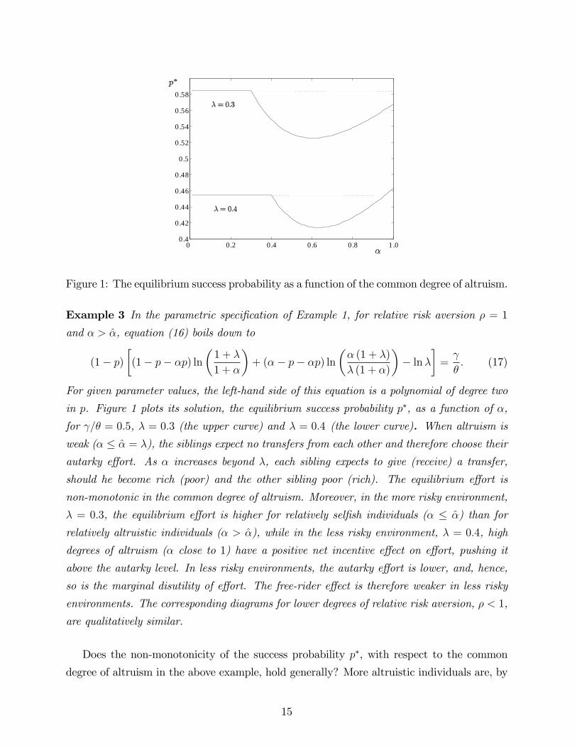
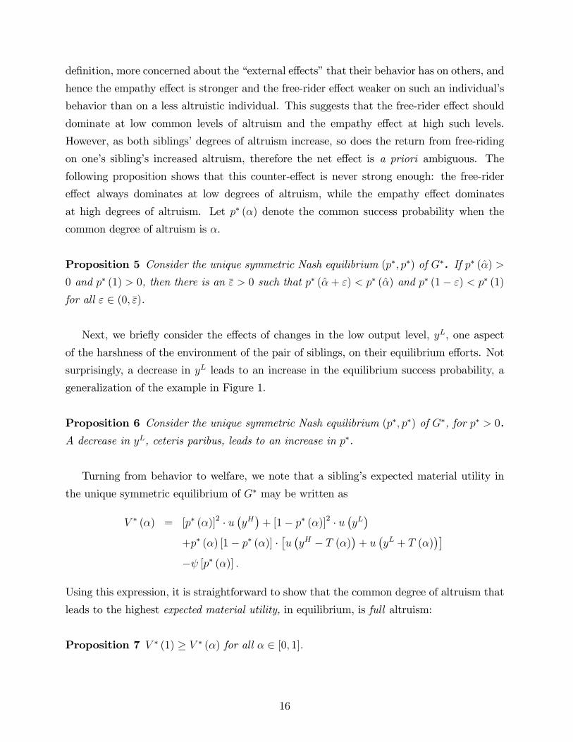
Figure 1: The equilibrium success probability as a function of the common degree of altruism.
Example 3 In the parametric specification of Example 1, for relative risk aversion ρ = 1
and α > α, equation (16) boils down to
(1− p)[(1− p− αp) ln
(1 + λ
1 + α
)+ (α− p− αp) ln
(α (1 + λ)
λ (1 + α)
)− lnλ
]=γ
θ. (17)
For given parameter values, the left-hand side of this equation is a polynomial of degree two
in p. Figure 1 plots its solution, the equilibrium success probability p∗, as a function of α,
for γ/θ = 0.5, λ = 0.3 (the upper curve) and λ = 0.4 (the lower curve). When altruism is
weak (α ≤ α = λ), the siblings expect no transfers from each other and therefore choose their
autarky effort. As α increases beyond λ, each sibling expects to give (receive) a transfer,
should he become rich (poor) and the other sibling poor (rich). The equilibrium effort is
non-monotonic in the common degree of altruism. Moreover, in the more risky environment,
λ = 0.3, the equilibrium effort is higher for relatively selfish individuals (α ≤ α) than for
relatively altruistic individuals (α > α), while in the less risky environment, λ = 0.4, high
degrees of altruism (α close to 1) have a positive net incentive effect on effort, pushing it
above the autarky level. In less risky environments, the autarky effort is lower, and, hence,
so is the marginal disutility of effort. The free-rider effect is therefore weaker in less risky
environments. The corresponding diagrams for lower degrees of relative risk aversion, ρ < 1,
are qualitatively similar.
Does the non-monotonicity of the success probability p∗, with respect to the common
degree of altruism in the above example, hold generally? More altruistic individuals are, by
15
definition, more concerned about the “external effects”that their behavior has on others, and
hence the empathy effect is stronger and the free-rider effect weaker on such an individual’s
behavior than on a less altruistic individual. This suggests that the free-rider effect should
dominate at low common levels of altruism and the empathy effect at high such levels.
However, as both siblings’degrees of altruism increase, so does the return from free-riding
on one’s sibling’s increased altruism, therefore the net effect is a priori ambiguous. The
following proposition shows that this counter-effect is never strong enough: the free-rider
effect always dominates at low degrees of altruism, while the empathy effect dominates
at high degrees of altruism. Let p∗ (α) denote the common success probability when the
common degree of altruism is α.
Proposition 5 Consider the unique symmetric Nash equilibrium (p∗, p∗) of G∗. If p∗ (α) >
0 and p∗ (1) > 0, then there is an ε > 0 such that p∗ (α + ε) < p∗ (α) and p∗ (1− ε) < p∗ (1)
for all ε ∈ (0, ε).
Next, we briefly consider the effects of changes in the low output level, yL, one aspect
of the harshness of the environment of the pair of siblings, on their equilibrium efforts. Not
surprisingly, a decrease in yL leads to an increase in the equilibrium success probability, a
generalization of the example in Figure 1.
Proposition 6 Consider the unique symmetric Nash equilibrium (p∗, p∗) of G∗, for p∗ > 0.
A decrease in yL, ceteris paribus, leads to an increase in p∗.
Turning from behavior to welfare, we note that a sibling’s expected material utility in
the unique symmetric equilibrium of G∗ may be written as
V ∗ (α) = [p∗ (α)]2 · u(yH)
+ [1− p∗ (α)]2 · u(yL)
+p∗ (α) [1− p∗ (α)] ·[u(yH − T (α)
)+ u
(yL + T (α)
)]−ψ [p∗ (α)] .
Using this expression, it is straightforward to show that the common degree of altruism that
leads to the highest expected material utility, in equilibrium, is full altruism:
Proposition 7 V ∗ (1) ≥ V ∗ (α) for all α ∈ [0, 1].
16
The intuition is simple: fully altruistic individuals completely internalize the external
effect of their own behavior on their sibling’s material utility.16 Hence, siblings’incentives
are perfectly aligned, with each sibling acting like a utilitarian social planner. For lower
degrees of altruism, however, their incentives are imperfectly aligned and there is room for
some free-riding. From this, it is not diffi cult to show that the expected equilibrium outcome
of the interaction between two equally altruistic siblings is, ex ante, Pareto effi cient, in terms
of their (imperfectly or perfectly) altruistic preferences, if and only if both siblings are fully
altruistic.
Corollary 1 The symmetric Nash equilibrium (p∗, p∗) of G∗ is Pareto effi cient if and only
if α = 1.
At first sight, it may come as a surprise that the outcome is ineffi cient even when the
siblings are purely selfish (α = 0). Should not the independent strife of selfish individuals
lead to a Pareto-effi cient outcome? The explanation is that both individuals’utility can
be increased by keeping their common success probability at its equilibrium level, but by
having the rich sibling transfer a small amount to the poor sibling, whenever they end up
with distinct outputs. Such consumption smoothing across states is beneficial, ex ante,
because of the assumed risk aversion (concavity in the utility from consumption). Hence,
two selfish siblings would prefer to write such an (incomplete and mutual) insurance contract,
also involving their efforts, had this been possible.
While very high levels of altruism are beneficial, it is a non-trivial matter whether mod-
erate levels of altruism are beneficial in terms of the expected material utility. As was shown
above, the success probability, and therefore also the expected output, declines as altruism
increases from an initially moderate level. It turns out, however, that the expected material
utility increases:
Proposition 8 If p∗ (α) > 0 there is an ε > 0 such that V ∗ (α + ε) > V ∗ (α) for all ε ∈(0, ε).
16Assuming that the siblings are fully altruistic is mathematically equivalent to assuming that they are
selfish, but that together they can commit to an effort level and a transfer from a rich individual to a poor
individual that maximize their joint expected material utility, a situation modelled by Arnott and Stiglitz
(1991).
17
In the proof of the proposition, we use V (α, β) to denote the expected material utility
obtained by an individual with altruism α in equilibrium play with a sibling with altruism
β:
V (α, β) = p (α, β) p (β, α)u(yH)
(18)
+ [1− p (α, β)] [1− p (β, α)]u(yL)
+p (α, β) [1− p (β, α)]u[yH − T (α)
]+ [1− p (α, β)] p (β, α)u
[yL + T (β)
]− ψ [p (α, β)] .
Here p : [0, 1]2 → (0, 1) is the function that to each pair of sibling altruism levels, (α, β),
specifies the equilibrium success probability of the α-altruist.17 Thus, if an individual has
altruism α and his or her sibling has altruism β, then p (α, β) is the individual’s own success
probability, and p (β, α) is that of the sibling. Such a pair of success probabilities, when
positive, necessarily satisfy the system of equations (13). Let A be the degrees of altruismα ∈ [0, 1] such that V : [0, 1]2 → R is differentiable at the point (α, α). It follows from (18)
that for α ∈ A the function p is differentiable at (α, α) as well. Let its partial derivatives
at such a point, with respect to its first and second arguments, be denoted p1 (α, α) and
p2 (α, α), respectively.
5 Evolutionarily stable family ties
A pair of siblings would fare best, in terms of their expected material utility, if they were both
fully altruistic. But if sibling altruism is a trait that is inherited from parent to child (where
inheritance could be cultural or genetic), is such a high degree of altruism stable against
“mutations” towards lower degrees of altruism? Here we propose a method to determine
stable degrees of altruism. In this exploration, we follow and extend somewhat Bergstrom’s
(1995, 2003) approach. More specifically, suppose that a child adopts its father’s or mother’s
degree of sibling altruism (“family values”), with equal probability for both events, and with
statistical independence.18 Thus, if the father’s degree of altruism is αf and the mother’s is
17We restrict attention to cases in which there is a unique equilibrium. Uniqueness holds, for instance, in
the parametric example in Section 2.1 (for details, see Alger and Weibull, 2007). The uniqueness assumption
will, in fact, be used only when α and β are (infinitesimally) close to each other.
18If the transmission is genetic, this corresponds to the sexual haploid reproduction case, where each
parent carries one copy of the gene, and the child inherits either the father’s or the mother’s gene. The
18
αm 6= αf , then, with probability 1/4 the two siblings will both have altruism αf , with the
same probability they will both have altruism αm, and with probability 1/2 one sibling will
have altruism αf and the other αm. As in Bergstrom’s (1995) model, mating is monogamous
and mate selection is random.19
5.1 Local evolutionary stability
Consider a sequence of successive, non-overlapping generations, living for one time period
each. In each time period, those individuals who survived to the age of reproduction mate
in randomly matched pairs. Each pair has exactly two children, and each sibling pair plays
a symmetric game once.20 This game may be the game in Subsection 2.2. In the first
generation, all individuals have the same degree of sibling altruism α ∈ [0, 1]. Suppose that
a “mutation”occurs in the second generation: a small population share of those who are
about to reproduce switch to another degree of altruism, α′ 6= α. Such a switch could be
caused by genetic drift, a cultural shift in family values, or it could be due to the immigration
of individuals with other family values. Random matching of couples takes place as before
and reproduction occurs. We call the “incumbent”degree of altruism α evolutionarily stable
against α′ if a child carrying the incumbent degree of altruism obtains, on average, a higher
material utility than a child carrying the mutant degree, for all suffi ciently small population
shares of the “mutant” degree of altruism, α′. The “incumbent” degree α is (globally)
evolutionarily stable if this holds for every α′ 6= α.
As we will presently see, the condition for the above-mentioned incumbent degree of
altruism α to be (globally) evolutionarily stable against a mutant degree α′ 6= α boils down
human species uses sexual diploid reproduction: then, each individual has two sets of chromosomes; one set
is inherited from the father, and the other from the mother. Whether a gene is expressed or not depends
on whether it is recessive (two copies are needed for the gene to be expressed), or dominant (one copy is
suffi cient for the gene to be expressed). Bergstrom’s (2003) analysis of games between relatives shows that
the condition for a population carrying the same gene to resist the invasion by a mutant gene in the haploid
case is the same as the condition for a population carrying the same recessive gene to resist the invasion by
a dominant mutant gene in the diploid case.
19In Section 6 we generalize the evolutionary process to allow for assortative mating as well as societal
influences.
20Somewhat more generally, each pair may have an even number of children and they interact in pairs.
19
to the following inequality:
V (α, α) >1
2[V (α′, α) + V (α′, α′)] , (19)
where V (α, β) denotes the expected material utility to an individual with altruism α whose
sibling has altruism β (see (18)). Formally, we define a degree of sibling altruism α ∈ [0, 1]
to be evolutionarily stable if it meets (19) for all α′ 6= α.21
To see that (19) is suffi cient for evolutionary stability as informally defined above, note
that the left-hand side, V (α, α), approximates the expected material utility to a child with
the incumbent degree of altruism, α. For if the population share of mutants in the parent
generation, ε > 0, is close to zero, then, with near certainty, both parents of this child are
α-altruists, implying that the child’s sibling is also almost surely an α-altruist. Likewise,
the expression on the right-hand side approximates the expected material utility to a child
with the mutant degree of altruism, α′. Because, for ε close to zero, such a child almost
certainly has exactly one parent with the mutant degree of altruism (the probability that
both parents are mutants is an order of magnitude smaller, ε2, and the probability that none
is, is zero). Therefore, with probability close to 1/2, this child’s sibling has the incumbent
degree of altruism, α, and, with the complementary probability, the sibling has the mutant
degree of altruism, α′.22
The process by which mutations appear in a population may affect the extent to which
the mutant degree of altruism differs from the incumbent degree. In particular, “cultural
drift”in a society’s values may arguably lead to smaller differences between incumbents and
mutants, while immigration from another community or society may sometimes give rise to
21Bergstrom (1995, 2003) derives a condition similar to (19) in a slightly different model, in which each
individual is programmed to play a strategy in a symmetric two-player game. Bergstrom shows that for a
sexual haploid species, a suffi cient condition for a population consisting of x-strategists to be stable against
a small invasion of y-strategists is
Π(x, x) >1
2Π(y, x) +
1
2Π(y, y),
where Π(s, s′) denotes the payoff to strategy s against strategy s′.
22The exact condition for evolutionary stability, as informally defined in the text above, is that for every
α′ there exists an ε ∈ (0, 1) such that
(2− ε)V (α, α) + εV (α, α′) > (1− ε)V (α′, α) + (1 + ε)V (α′, α′)
for all ε ∈ (0, ε). By continuity, (19) is suffi cient for this, and its weak-inequality version is necessary.
20
larger such differences. Thus, the relevant evolutionary stability criterion against “cultural
drift”is a local version of the above definition. Formally:
Definition 1 A degree of altruism α ∈ [0, 1] is locally evolutionarily stable if (19) holds
for all α′ 6= α in some neighborhood of α.
Let us elaborate the notions of evolutionary stability and local evolutionary stability a bit.
First, note that a degree of altruism α is evolutionarily stable if and only if the right-hand
side of (19), viewed as a function of α′ ∈ [0, 1], has its unique global maximum at α′ = α.
Second, a degree of altruism α is locally evolutionarily stable if and only if the right-hand
side of (19), again viewed as a function of α′ ∈ [0, 1], has a strict local maximum at α′ = α.
Recalling that A is the set of degrees of altruism α ∈ [0, 1] such that V : [0, 1]2 → R, definedin (18), is differentiable at the point (α, α), define D : A → R by
D (α) = V1(α, α) +1
2V2(α, α), (20)
where Vk is the partial derivative of V with respect to its k’th argument, for k = 1, 2. For
any degree of altruism α ∈ A, D (α) is the derivative of the right-hand side of (19), viewed
as a function of α′, evaluated at α′ = α. We will refer to the function D as the evolutionary
drift function.
If the incumbent degree of altruism in a society is α ∈ A, then D (α) dα is the marginal
effect of a slight increase in a mutant’s degree of altruism, from α to α + dα, on its child’s
expected material utility (achieved in the child’s equilibrium play with its sibling) if the child
inherits its mutant parent’s degree of altruism. The first term is the effect of an increase
in the child’s own altruism on his or her expected material utility, whereas the second term
is the effect of an increase in the child’s sibling’s altruism, multiplied by one half – the
conditional probability that also the sibling is a mutant.
If D (α) > 0, then the mutant child, if slightly more altruistic than the incumbent
population, will outperform the incumbents’children in terms of expected material utility.
Likewise, if D (α) < 0, then it is instead a mutant child who is slightly less altruistic than the
incumbents that will outperform the incumbents’children. Hence, in order for an incumbent
degree of altruism α ∈ A to be locally evolutionarily stable, it is necessary that D (α) = 0.
Let int (A) ⊂ A be the set of interior points in A, that is, degrees of altruism α such that V
is continuously differentiable at all points (α′, α′) near (α, α). For such degrees of altruism
21
more can be said:23
Proposition 9 A necessary condition for a degree of altruism α ∈ A to be locally evolu-
tionarily stable is D (α) = 0. A necessary and suffi cient condition for a degree of altruism
α ∈ int (A) to be locally evolutionarily stable is (i)-(iii), where:
(i) D (α) = 0
(ii) D (α′) > 0 for all nearby α′ < α
(iii) D (α′) < 0 for all nearby α′ > α.
In other words: wherever the evolutionary drift function is well-defined, a necessary
condition for local evolutionary stability is that there be no drift, and that there be upward
(downward) drift at slightly lower (higher) altruism levels. Clearly, if D is differentiable at
α and satisfies (i), then D′ (α) < 0 implies (ii) and (iii).
5.2 Application to the present sibling interaction
Here, we derive the drift function for the case where siblings interact according to the model
analyzed in Sections 2-4. Recall from Proposition 3 that if p (α, β) > 0 and p (α, β) > 0,
then p1 (α, β) > 0 and p2 (α, β) < 0 whenever α, β > α. Straightforward calculations based
on (18) and the envelope theorem lead to:
Lemma 1 For any α ∈ int (A) with p (α, α) > 0:
D (α) = (1/2− α) · F (α) + [(1/2− α) p1 (α, α) + (1− α/2) p2 (α, α)] ·G (α) (21)
where
F (α) = p (α, α) (1− p (α, α)) · u′[yL + T (α)
]T ′ (α)
and
G (α) = p (α, α) ·(u(yH)− u
[yH − T (α)
])+ [1− p (α, α)] ·
(u[yL + T (α)
]− u
(yL)).
23This follows from the fact that local evolutionary stability is equivalent with local strict maximization
of the right-hand side of (19).
22
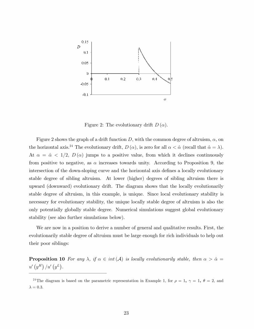
Figure 2: The evolutionary drift D (α).
Figure 2 shows the graph of a drift functionD, with the common degree of altruism, α, on
the horizontal axis.24 The evolutionary drift, D (α), is zero for all α < α (recall that α = λ).
At α = α < 1/2, D (α) jumps to a positive value, from which it declines continuously
from positive to negative, as α increases towards unity. According to Proposition 9, the
intersection of the down-sloping curve and the horizontal axis defines a locally evolutionary
stable degree of sibling altruism. At lower (higher) degrees of sibling altruism there is
upward (downward) evolutionary drift. The diagram shows that the locally evolutionarily
stable degree of altruism, in this example, is unique. Since local evolutionary stability is
necessary for evolutionary stability, the unique locally stable degree of altruism is also the
only potentially globally stable degree. Numerical simulations suggest global evolutionary
stability (see also further simulations below).
We are now in a position to derive a number of general and qualitative results. First, the
evolutionarily stable degree of altruism must be large enough for rich individuals to help out
their poor siblings:
Proposition 10 For any λ, if α ∈ int (A) is locally evolutionarily stable, then α > α =
u′(yH)/u′(yL).
24The diagram is based on the parametric representation in Example 1, for ρ = 1, γ = 1, θ = 2, and
λ = 0.3.
23
Incumbents with α ≤ α do not give any transfers. Since a mutant sibling with altruism
α′ near α does not give any transfer either, and hence it obtains the same expected material
utility as a sibling with the incumbent degree of altruism, α, it follows that no degree of
altruism α ≤ α is locally evolutionarily stable.
In the light of Hamilton’s rule (Hamilton, 1964a), mentioned in the introduction, one
might expect α = 1/2 to be the stable degree of kinship altruism. This is never true here,
however. In fact, an evolutionarily stable degree of altruism must be smaller than 1/2:
Proposition 11 If α ∈ int (A) is locally evolutionarily stable, then α < 1/2.
Consider a population where the degree of altruism is one half (or higher) and where the
equilibrium transfer from a rich to a poor sibling is positive. Such a population would be
vulnerable to the “invasion”by slightly less altruistic mutants: for any α ≥ 1/2 (and α > α),
D (α) < 0 (see equation (21)).
Propositions 10 and 11 together imply that there exists an evolutionarily stable degree
of altruism only if α < 1/2, or, equivalently, only if
λ < λ =1
yH(u′)
−1 [2u′(yH)]. (22)
This condition says that the environment is such that the critical degree of altruism for a
transfer to occur is lower than Wright’s coeffi cient of relationship between the siblings. In
gentle environments (where λ ≥ λ), the marginal utility at the low output is so close to the
marginal utility at the high output level that siblings with altruism α = 1/2 do not give any
transfers to each other, and from Proposition 10 this cannot be stable.
The result in Proposition 11 is due to the “strategic externality” that one sibling’s al-
truism exerts on the other’s choice of effort: each sibling adjusts his or her productive effort
not only to the exogenous environment, but, also, to the anticipated transfer from the other
sibling. To see that this “strategic externality” influences what degree of altruism is evo-
lutionarily stable, suppose that both siblings’ success probabilities instead were fixed, at
some exogenously given level. What levels of sibling altruism α would then be evolutionarily
stable? An application of Proposition 9 provides the answer:
Corollary 2 Suppose that λ < λ and that efforts are exogenously fixed and equal. Then the
unique evolutionarily stable degree of sibling altruism is α = 1/2.
24
0.1 0.2 0.3 0.4
2.5
3.5
4.5
5.5
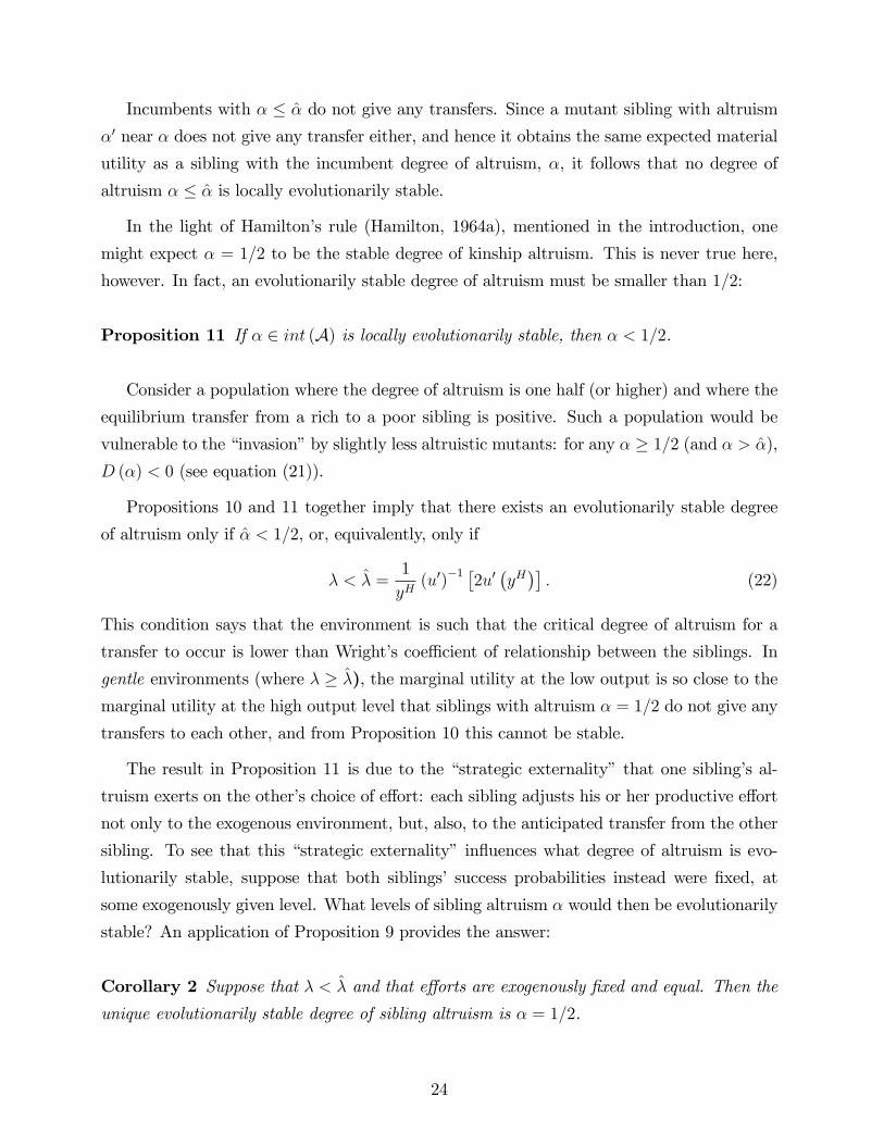
Figure 3: The evolutionarily stable degree of altruism as a function of output variability λ
and return to effort θ.
Our result for evolutionary stability thus confirms Hamilton’s rule in settings in which
the only interaction between siblings is “pie division,”that is, how a resource of given size
will be split. In the present model, the siblings not only divide the “pie,”but also influence
its size, by way of their (costly) efforts. It is this additional and strategic element that drives
down the evolutionary stable degree of sibling altruism, below 1/2. This raises two questions:
“By how much?”and “How does this depend on other aspects of the environment in which
they live?”Given the analytical complexity, we resort to numerical simulations.
5.3 Evolutionary comparative statics
Here, we use the parametric specification in Example 1 to explore how different aspects of
the environment may affect the evolutionary stability of different degrees of altruism, and
thereby also indirectly effort, income, and material welfare. In order to limit the number of
parameters, we henceforth set γ = ρ = 1. In this case λ = 1/2, see equation (22).
Figure 3 shows the stable degree of altruism as a function of the parameters λ and θ,
where a high λ means a less risky environment (the low output level being a larger share of
the high output level) and a high θ means a higher (absolute and marginal) return to effort
(in terms of the resulting probability for the high output level). We see that higher degrees
of altruism are selected for in environments that are milder in the sense of having higher
25
0.1 0.2 0.3 0.4
2.5
3.5
4.5
5.5
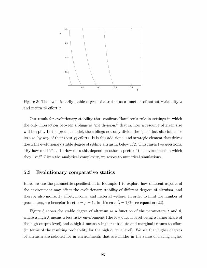
Figure 4: Equilibrium effort x∗ as a function of output variability λ and return to effort θ,
and for stable altruism levels.
λ and/or θ. This might, at first sight, appear counterintuitive, since risk sharing between
siblings would seem to have a lower survival value in milder environments. However, this
intuition neglects the incentive effect of the environment on effort: that the “size of the pie”is
not exogenous. Indeed, the milder the environment, the less vulnerable is a population with
high kinship altruism to an “invasion”by less altruistic mutants. For example, consider an
individual, A, whose sibling, B, is less altruistic. A suffers doubly from the relative selfishness
of B: the latter both makes a lesser effort (Proposition 3) and gives a lower transfer, when B is
rich and A poor. The altruistic individual is thus more likely to have to help out his sibling,
is less likely to be helped out, and receives a lower transfer, than if his sibling had been
like him. Since, in milder environments, both siblings make lower efforts (Proposition 6), a
slightly less altruistic sibling B may have less to gain from his free-riding on the altruistic
individual A, in milder environments.
In the subsequent diagrams, we have calculated the equilibrium effort and income as
indirect functions of the environment (λ, θ), by first letting the degree of sibling altruism
adapt to its unique evolutionarily stable value in each environment, and then letting the
siblings choose their corresponding equilibrium efforts. Figure 4 shows the resulting effort,
x∗, as such an indirect function of the environment (λ, θ). For a given value of θ, siblings
(with the corresponding evolutionarily stable degree of altruism) exert less work effort in
environments with lower output variability (higher λ). Hence, in milder environments their
26
0.1 0.2 0.3 0.4
2.5
3.5
4.5
5.5
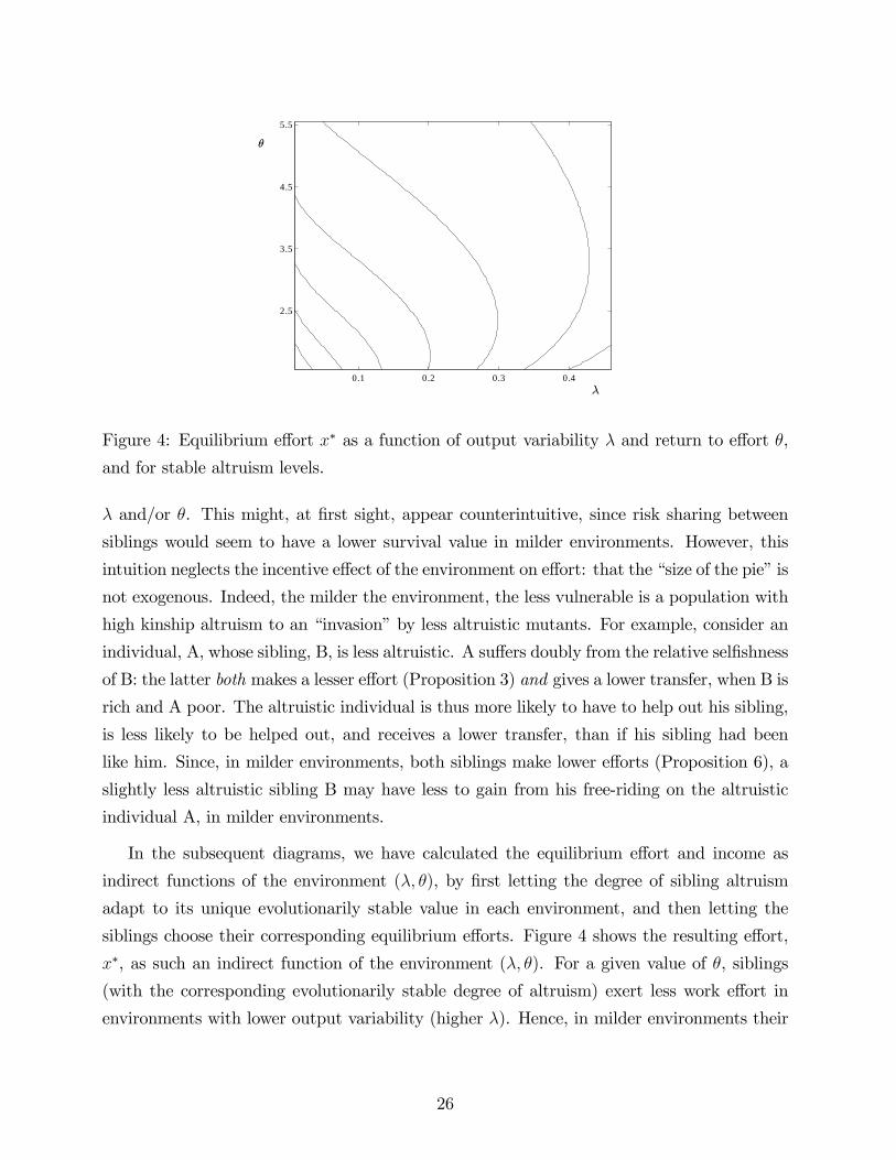
Figure 5: Equilibrium income Y ∗ as a function of output variability λ and return to effort
θ, and for stable altruism levels.
family ties are stronger and they work less hard. The effect of θ, the return to effort,
is not as clear-cut: for some values of λ, the equilibrium effort, as an indirect function
of the environment, is non-monotonic in θ. This is due to two opposing effects: a sort
of substitution effect and a sort of income effect. Ceteris paribus, an increase in θ has a
positive incentive (substitution) effect, but, in the new and slightly milder environment, the
stable level of altruism is a bit higher, and this has a disincentive (income) effect on effort.
Our numerical simulations show that the equilibrium effort level, given the associated stable
degree of altruism, is lower than the corresponding autarky effort level, for all values of θ.
The lower effort exerted in milder environments does not always yield lower incomes.
Indeed, when family ties adapt to the environment, the expected income may increase as
the environment becomes milder, see Figure 5. However, even if the expected income is
lower in a milder environment (with higher λ, say), and people thus are poorer, they may
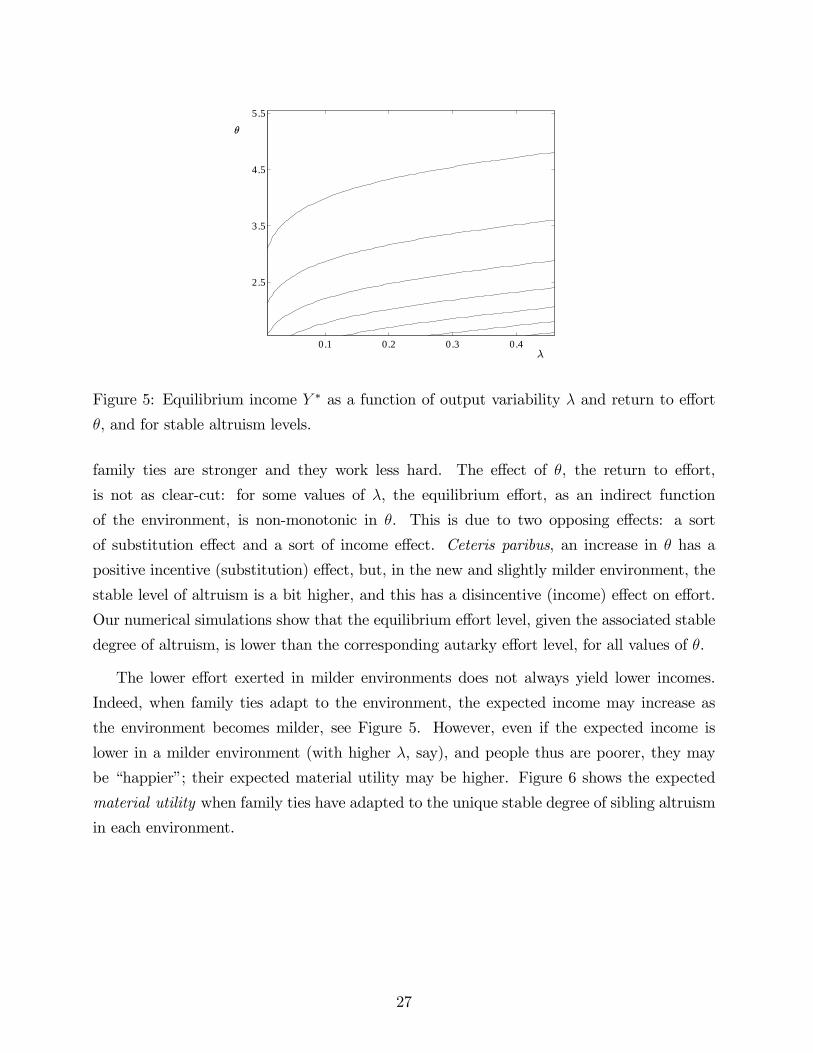
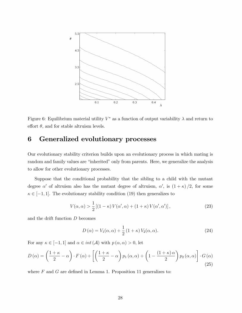
be “happier”; their expected material utility may be higher. Figure 6 shows the expected
material utility when family ties have adapted to the unique stable degree of sibling altruism
in each environment.
27
0.1 0.2 0.3 0.4
2.5
3.5
4.5
5.5
Figure 6: Equilibrium material utility V ∗ as a function of output variability λ and return to
effort θ, and for stable altruism levels.
6 Generalized evolutionary processes
Our evolutionary stability criterion builds upon an evolutionary process in which mating is
random and family values are “inherited”only from parents. Here, we generalize the analysis
to allow for other evolutionary processes.
Suppose that the conditional probability that the sibling to a child with the mutant
degree α′ of altruism also has the mutant degree of altruism, α′, is (1 + κ) /2, for some
κ ∈ [−1, 1]. The evolutionary stability condition (19) then generalizes to
V (α, α) >1
2[(1− κ)V (α′, α) + (1 + κ)V (α′, α′)] , (23)
and the drift function D becomes
D (α) = V1(α, α) +1
2(1 + κ)V2(α, α). (24)
For any κ ∈ [−1, 1] and α ∈ int (A) with p (α, α) > 0, let
D (α) =
(1 + κ
2− α
)·F (α) +
[(1 + κ
2− α
)p1 (α, α) +
(1− (1 + κ)α
2
)p2 (α, α)
]·G (α)
(25)
where F and G are defined in Lemma 1. Proposition 11 generalizes to:
28
Proposition 12 Suppose that λ < λ. If α ∈ int (A) is locally evolutionarily stable, then
α < α ≤ 1/2 + κ/2, and α is increasing in κ. In particular, α may exceed 1/2 if and only if
κ > 0. Moreover, α = 1 is a locally stable degree of altruism if κ = 1.
The more likely a mutant is to have a mutant sibling, the higher is the stable degree of
altruism. A relatively selfish mutant is worse off the higher the probability is that its sibling
is also relatively selfish, for such a mutant is more likely to receive a low transfer and is
also less likely to receive a transfer (since the empathy effect is weaker on a relatively selfish
sibling).
6.1 Assortative mating
Suppose that grown-ups have a tendency towards assortative mating. With probability
µ ∈ [0, 1] a given mutant grown-up is selective and settles only for a match with another
mutant, while with the complementary probability, 1−µ, the mutant is non-selective and hasa randommatch.25 For a small population share ε > 0 of mutants, the conditional probability
that the sibling to a child with the mutant degree α′ of altruism also has altruism α′ is then
approximately equal to (1− µ) /2 + µ (instead of 1/2). Equation (25) and Proposition 12
may be applied, by setting κ = µ. When µ > 0, that is, when individuals are more likely
to marry someone with the same “family values,”then the marginal fitness effect on a child
from a mutation towards a slightly higher level of sibling altruism is higher, and, as a result,
so is the evolutionarily stable degree of such altruism.
6.2 Social evolution
Suppose that mating is random but children may be influenced by the values in the sur-
rounding society. With probability 1−ζ a child “inherits”one of its parents’degree of familyaltruism (“parental influence”), with equal probability for both parents. With probability
ζ ∈ [0, 1], the child imitates a randomly drawn grown-up from the population at large. For
a small population share ε > 0 of grown-up mutants, the conditional probability that the
sibling to a child with the mutant degree α′ of altruism also has altruism α′ is then close
to (1− ζ) /2. Equation (25) and Proposition 12 apply, with κ = −ζ. A higher likelihood ζ
25This formalization is in line with Cavalli-Sforza and Feldman (1981), see also Wright (1921) and
Bergstrom (2003).
29
that children’s family values are influenced by society at large, rather than by their parents,
implies that the marginal value to a child’s fitness, from a mutation to a slightly higher level
of kinship altruism, is lower, since this decreases the likelihood that the child’s sibling also
is a mutant. Consequently, the evolutionarily stable degree of altruism is lower.
7 Discussion
Our basic model is very simple. Here we briefly discuss some variations of our assumptions.
7.1 Commitment
In our base-line model, there is no possibility to precommit to efforts or transfer levels.
Suppose that both siblings are committed to effort level, x > 0. Such commitment may be
the result of strong social norms concerning work effort (“work ethic”), social norms that
may be internalized or socially sanctioned. The success probabilities would then be fixed,
so an increase in an individual’s degree of altruism could only lead to an increase in his or
her (voluntary) transfer to his or her sibling. Corollary 2 implies that, with random mating
and pure parental influence, the unique evolutionarily stable level of altruism would then be
α = 1/2, irrespective of the committed effort level x > 0: Hamilton’s rule would apply.
Next, suppose that a rich sibling is committed to transfer T ∈(0, yH
)to a poor sibling.
Such commitment may again be the result of social norms.26 The preceding analysis may be
applied directly, by setting T (α) ≡ T (and thus T ′ (α) = 0). Let p (α, α) denote the effort
in the unique symmetric equilibrium of the corresponding game, when both individuals have
sibling altruism α. Proposition 3 still holds; an increase in own altruism leads to an increase
in effort. Interestingly, however, if instead the common degree of altruism is increased, the
empathy effect always outweighs the free-rider effect, at the margin. The non-monotonicity
result in Proposition 5 does not carry over to this setting; with an exogenous transfer T ,
the unique symmetric equilibrium effort is increasing in the common degree of altruism.27
26We refer to Alger and Weibull (2008) for an analysis of what level of such commitment would be stable
as a social norm, and how the resulting intrafamily risk sharing compares to risk sharing by way of formal
insurance systems.
27To see this, set T ′ (α) = 0 in equation (33), in the proof of Proposition 5.
30
Moreover, the drift function now becomes
D (α) = [(1/2− α) p1 (α, α) + (1− α/2) p2 (α, α)] ·G (α) (26)
where p1 (α, α) and p2 (α, α) are the two partial derivatives of the equilibrium success prob-
ability p (α, β), evaluated at β = α. We obtain
G (α) = p (α, α) ·[u(yH)− u
(yH − T
)]+ [1− p (α, α)] ·
[u(yL + T
)− u
(yL)].
Since p1 (α, α) > 0 and p2 (α, α) < 0, equation (26) implies that the conclusion of Proposition
11 holds up when the transfer is exogenously fixed: any evolutionarily stable degree of
altruism α is necessarily lower than 1/2 (under randommating and purely parental influence).
7.2 Repetition
Above, we have analyzed a two-stage interaction that takes place only once. An interesting
extension would be to let this interaction occur repeatedly over time. Suppose that the
interaction takes the form of an infinitely repeated game between two (altruistic or selfish)
siblings, with equal discounting. Under perfect monitoring, any feasible and individually
rational outcome (defined in terms of their potentially altruistic preferences) would then be
achievable in subgame perfect equilibrium, if the siblings were suffi ciently patient. Repeated
play of the equilibrium of our baseline model would constitute one of these subgame perfect
equilibria, for all discount factors. However, the standard repeated-games model might
not be fully satisfactory. First, if output is storable, then stored output (wealth) would
constitute a state-variable of potential strategic relevance, and hence the long-run game
would not be a repeated game, but a stochastic game. Second, finite life spans and age-
dependent conditional survival probabilities would tend to make siblings less patient as
they grow older, leading to a reduction of the set of subgame-perfect equilibria, though
presumably still containing repeated play of the baseline equilibrium analyzed here. Despite
these complications, repetition is certainly an important aspect well worth analyzing: a
subject that we leave for future studies.
7.3 Preference evolution vs. strategy evolution
We have analyzed the evolutionary stability of preferences, rather than of strategies, and
we focused on a setup where the players of the game are not randomly matched. Each
31
of these two deviations from the standard approach has been analyzed separately before.
The so-called indirect evolutionary approach (see, e.g., Güth and Peleg, 2001, and Heifetz,
Shannon, and Spiegel, 2007) concerns the evolutionary stability of preferences under random
matching, whereas Bergstrom (1995) analyzes the evolutionary stability of strategies when
the players are siblings, so that their “strategy types”are correlated in a specific way.
To clarify how these approaches differ from ours, reconsider the two-stage interaction ana-
lyzed in Sections 2-4. Had we studied the evolutionary stability of preferences with randomly
matched players, then pure selfishness would have been selected for, since mutants would
be almost sure to be matched with incumbents. What if we had studied strategy evolution
with non-randomly matched players? A pure strategy in this symmetric two-player game is
an effort level and a transfer function that assigns transfers to each of the four second-period
states. Assume that strategies, rather than degrees of altruism, are inherited from parent
to child. Evolutionary stability of strategies would lead to a condition formally identical to
(19), with the incumbent degree of altruism, α, replaced by an incumbent strategy, s, and
with the mutant degree of altruism, α′, replaced by a mutant strategy, s′. This approach
would differ from ours in two important respects. First, while, in our model, incumbents
and mutants adapt their own behavior to their sibling’s “preference type,”the behavior of
an incumbent or mutant in the strategy approach is independent of the sibling’s “strategy
type.”Secondly, in our model, a mutant’s degree of altruism (given the sibling’s “preference
type”) determines both the mutant’s transfer and effort. This restricts the set of possible
mutant behaviors. By contrast, in a model where individuals inherit strategies, the set of
possible mutant behaviors would be richer; any mutant effort could be combined with any
transfer function. Due to these differences, it is a non-trivial matter whether the strategy
approach would lead to the same evolutionarily stable behaviors as our approach. On the one
hand, the richer set of mutant behaviors would make it “harder”for any incumbent behavior
to be stable in the strategy approach. On the other hand, the inability of mutants to adjust
their behavior would make it “easier”for an incumbent behavior to be stable in the strategy
approach. We feel that the preference approach is more relevant than the strategy approach
in applications to human siblings, who have the cognitive capacity and “social intelligence”
to understand each other and adjust to each others’personality.
32
7.4 Public insurance
In our analysis, risk was pooled within the family only. This was arguably the case for many
societies throughout human history, prior to the advent of insurance arrangements beyond
the family sphere. As such, the analysis indicates how intrafamily altruism may have evolved
in the past. Here, we indicate how our analysis may be extended to allow for compulsory
redistribution/insurance systems that pool the risks of a large group of individuals.
Suppose that after outputs are realized, but before transfers are made, each rich individual
pays an income tax or insurance premium, ∆ ·yH , and every poor individual receives a publictransfer or indemnity (net of the premium), δ ·yL > 0. For exogenously given values of δ and
∆, our analysis can be directly applied, by way of replacing yH with (1−∆) yH , and yL with
(1 + δ) yL < (1−∆) yH in equations (7), (8), and (16). From the individual’s viewpoint it
is as if λ = yL/yH were replaced by
λδ,∆ =1 + δ
1−∆· λ > λ.
This has a disincentive effect: an increase in λ induces lower efforts. Moreover, the introduc-
tion of social insurance will crowd out intrafamily transfers, perhaps even eliminate them.
Our evolutionary analysis suggests that an increase in λ, due to the introduction of public
redistribution/insurance, may lead to a higher degree of sibling altruism, unless intrafamily
transfers are completely crowded out. We also note that lower institutional quality may lead
to stronger family ties. To see this, compare two identical societies with different insurance
systems, say (δ,∆) and (δ′,∆′) with δ′ < δ and ∆′ > ∆. The second society has lower
institutional quality, in the sense that it taxes more and delivers less. According to our
evolutionary comparative-statics analysis, family ties will tend to be stronger in the latter.
While each individual takes δ and ∆ as exogenous and fixed when choosing effort, these
parameters may, in a policy-formation process, depend on each other through a governmental
budget-balance condition. From each dollar collected as a tax or insurance premium from
the rich, let η ∈ [0, 1] be the share that reaches the poor. The rest goes to administrators and
government offi cials. If all individuals choose the same success probability p, the expected
per capita tax revenue is ηp∆yH , while the expected per capita transfer or indemnity to those
with low output is (1− p) δyL. Aggregate (expected) budget balance, given the “leakage”factor η, requires that these two amounts are equal, or, equivalently, that
p =δλ
η∆ + δλ, (27)
33
where λ = yL/yH . Replacing p by the equilibrium success probability in this equation
determines the set of budget-balanced policies (δ,∆), given α and η. Let M (α, η) be the
maximum expected material utility that may be achieved across the set of all feasible policies,
given α and η. Clearly M (α, η) is increasing in the institutional quality parameter η, given
α. As before, let V ∗ (α) be the expected material utility in our base-line model without
public insurance/redistribution. For each α, let
η (α) = min η ∈ [0, 1] : M (α, η) ≥ V ∗ (α) .
This set defines the lowest institutional quality η for which the optimal public social insurance
system is superior to laissez-faire. If η (α) > η (α′) for some α and α′, then a society consisting
of α′-altruists will more likely adopt a public social insurance system, ceteris paribus, than
a society with α-altruists, since the optimal public policy is superior to laissez-faire for a
wider range of institutional qualities in the former than in the latter society. Preliminary
numerical simulations suggest that harsher environments may induce lower degrees of sibling
altruism and a wider range of parameters under which public social insurance is superior to
laissez-faire – a topic for future research.
8 Conclusion
Family ties are arguably stronger in some parts of the world than in others, and there is
empirical evidence that the strength of family ties may endure for several generations after
changes in the environment.28 This suggests that current differences in family ties may
be due to differences in the distant past, perhaps even prior to the industrial revolution.
These observations prompted us to ask first, how family ties affect economic outcomes,
and, second, whether evolutionary forces may have shaped family ties differently in different
environments. We focused on the family’s role as sole insurance provider for its members.
We modelled a family as a pair of mutually altruistic siblings, who may provide partial and
informal insurance to each other by way of voluntary transfers. The siblings choose their
risk-reducing efforts, anticipating possible future transfers between them. We found that,
28U.S. data collected by Keefe et al, (1979) indicates that second and third generation Mexican-American
(people of Mexican descent but born in the U.S.) families have stronger kinship ties than white Anglo
families, even after controlling for many variables. Using another data set, Gonzales (1998) shows that
Mexican-Americans tend to live closer to, and have more contact with, kin than Anglos, even after several
generations in the U.S.
34
in our model, altruism is a double-edged sword: it enhances the extent to which individuals
internalize the external effects of their actions, but it also enhances free-riding. We found
that these two opposing effects of altruism on effort, the free-rider effect and the empathy
effect, result in a risk-reducing effort that is non-monotonic in the extent of family risk
sharing. The presence of the free-rider and empathy effects are, arguably, quite a general
consequence of mutual altruism in situations that include some productive activity. How
far one can generalize our result, that the empathy effect outweighs the free-rider effect at
high levels of altruism while the opposite holds at intermediate levels of altruism, remains
an open question.
For a given level of intrafamily altruism, we studied how environmental factors, such
as output variability and the marginal return to effort, affect individual family members’
productive efforts. We then studied how evolutionary forces, be they genetic or sociocultural,
may affect the level of sibling altruism in a society. We showed that neither very weak
nor very strong family ties are stable against evolutionary drift. We also showed that the
degree of altruism dictated by Wright’s degree of relationship (1/2 for siblings) is unstable.
If a few individuals in such a society were to become slightly less altruistic towards their
kin, these individuals would do better in terms of material utility. We showed how this
generalizes Hamilton’s rule (Propositions 10-11) from exogenous to endogenous production,
and showed that intermediate degrees of family altruism are locally evolutionarily stable in
many environments. Numerical simulations suggested that the harsher the environment, the
weaker are the family ties.29
MaxWeber (1951) argued that “the great achievement of [...] the ethical and ascetic sects
of Protestantism was to shatter the fetters of the sib [the extended family]. These religions
established [...] a common ethical way of life in opposition to the community of blood, even
to a large extent in opposition to the family.” (p.237)30 Likewise, Banfield (1958) thought
that the “amoral familism”that he observed in certain parts of Italy was an impediment to
economic development. Macfarlane (1978, 1992) argues that the individualism that devel-
oped in northwestern Europe (in particular in England) was key in favoring the advent of
29The idea that individuals in a society may exhibit traits that depend on exogenous factors, such as
climate, goes back to Montesquieu (1748) at least.
30Some historians argue that religions may develop largely in response to underlying social factors, see,
e.g., Ozment (1975, 1992). Social factors may in turn evolve in response to exogenous factors, perhaps along
the lines suggested here.
35
markets and the industrial revolution.31 Our analysis suggests a reason why weaker family
ties may have developed in the arguably often harsher climates in the Protestant countries,
and how this may have induced stronger economic growth. This opens an avenue for future
theoretical and empirical research.
The results reported here are indeed derived under heroic simplifications. The sibling
interaction that we model is very simple and stylized. Its precise mathematical form, is, of
course, only one of many possibilities. However, we believe it is canonical for the interplay
between human effort and nature. Future work in this area may take many directions, in-
cluding those discussed in the preceding section. Moreover, we have focused on the evolution
of altruism in a society in an exogenous environment. Yet, many societies or groups compete
with each other for resources, sometimes by way of armed conflicts. A group or society with a
higher degree of internal altruism may then become materially richer and perhaps also more
successful in such conflicts. There could thus be selection of altruism at two levels, along
the lines proposed by Wilson and Wilson (2007). Using prehistoric evidence on violence,
Bowles (2009) finds that conflicts between groups indeed were common enough to favor the
evolution of altruism in such a fashion. Finally, it would be of interest to develop mod-
els that allow for more than two siblings, other kin-relations, and a richer menu of actions
and outcomes. We hope that the notion of local evolutionary stability of preferences, along
with the analytical machinery developed here, can be useful for further studies of social and
economic interactions.
31Macfarlane (1992) cites many studies showing that several centuries ago a large fraction of youngsters
in England were servants or laborers outside of the parental home, some leaving the parents at the age of
10. For instance, Kussmaul (1981) reports that as far back as 1380, more than half of men in East Anglian
villages were employees (servants or labourers), and Hajnal (1982) provides similar evidence for the 17th-
19th centuries. Thus, in 17th century England, “the unit of production was the husband and the wife and
hired labor, not children”(Macfarlane, 1978). By contrast, in southern and eastern Europe, during the same
period, hired labor was scarce and children would typically work on the parents’farm.
36
9 Appendix
9.1 Proposition 1
Let τ i : Ω →[0, yH
]be the function that defines, for every state ω ∈ Ω, the transfer that
individual i would like to make to his or her sibling if the latter makes no transfer to i. Then
τ i(ω) = 0 if u′(yi) ≥ αiu′(yj) for j 6= i, otherwise the optimal transfer τ i(ω) is positive and
equates i’s marginal material utility to that of his sibling’s when weighted by his own (i’s)
degree of altruism:
u′(yi − τ) = αiu′(yj + τ). (28)
Thus:
τ i(ω) = max 0, τ , (29)
where τ is uniquely defined by (28). Since the material utility function is separable in con-
sumption and effort, efforts play no role when determining the transfers, only outputs matter.
The claims in Proposition 1 follow from the following lemma:
Lemma 2 For each ω ∈ Ω, the transfer pair (τA(ω), τB(ω)) constitutes a Nash equilibrium
of G(ω). If αAαB < 1, then this equilibrium is unique. If αA = αB = 1, then there is a
continuum of Nash equilibria, all resulting in equal sharing of the total output.
Proof: We first prove that if αAαB < 1, in any equilibrium at most one transfer is strictly
positive. Suppose that αAαB < 1, and that (tA, tB) is a Nash equilibrium with tA, tB > 0.
Then the following two first-order conditions must both hold:
u′(yA − tA + tB) = αAu′(yB + tA − tB)
u′(yB + tA − tB) = αBu′(yA − tA + tB)
and hence
u′(yA − tA + tB) = αAαBu′(yA − tA + tB)
implying αAαB = 1, contradicting our hypothesis that αAαB < 1.
Suppose that αAαB < 1. Then the previous observation, together with (29), implies that
(tA, tB) = (τA(ω), τB(ω)) = (0, 0) is the unique equilibrium in the two states ω in which
yA = yB. The previous observation further implies that, in the states ω where yA 6= yB,
the individual with the low output yL gives no transfer, since u′(yL − τ) > αiu′(yH + τ)
37
for all αi ∈ [0, 1] and τ ≥ 0. Hence, if yA > yB, the unique Nash equilibrium of G (ω) is
(tA, tB) = (τA(ω), 0), and, if yB > yA, it is (tA, tB) = (0, τB(ω)).
Suppose now that αAαB = 1; then it is straightforward to verify the following claims:
• if yA > yB any (tA, tB) = (τA(ω) + ε, ε) is a Nash equilibrium of G (ω) for all ε ∈(0, yA − τA(ω))
• if yB > yA any (tA, tB) = (ε, τB(ω) + ε) is a Nash equilibrium of G (ω) for all ε ∈(0, yB − τB(ω))
• if yA = yB any (tA, tB) = (ε, ε) is a Nash equilibrium of G (ω) for all ε ∈ [0, yA].
9.2 Proposition 2
The first-order condition (8) implicitly defines the transfer t as a differentiable function of
λ. An application of the implicit function theorem gives
dt
dλ= −
αu′′(λyH + t
)αu′′ (λyH + t) + u′′ (yH − t) · y
H ,
where, by strict concavity of u, the ratio on the right-hand side is a number in the open unit
interval. Hence
d(λyH + t
)dλ
=
[1−
αu′′(λyH + t
)αu′′ (λyH + t) + u′′ (yH − t)
]· yH > 0,
andd(yH − t
)dλ
=αu′′
(λyH + t
)αu′′ (λyH + t) + u′′ (yH − t) · y
H > 0.
9.3 Proposition 3
First, assume that αA, αB < α. Then T (αA) = T (αB) = 0, and inspection of (14) shows that
the equation system (13) is independent of αA and αB. Hence, its solution set is unaffected
by a marginal increase in any one, or both, of these parameters.
Second, assume that condition (15) is met. Then the Jacobian of the equation system
(13) is non-null, a condition, which, by the Inversion Theorem (see, e.g., Theorem 41.8 in
Bartle, 1976), guarantees local uniqueness of the solution to (3). Suppose that αi > α, and
consider an increase in αi.
38
Step 1: First, we prove that, for each success probability of the other individual, pj,
individual i’s best response is strictly increasing in αi. From (13) and noting that (ψ′)−1 is
an increasing function, this claim holds if
∂g (pj, αi, αj)
∂αi> 0.
Using the first-order condition (8) for the transfer T (αi), we obtain:
∂g (pj, αi, αj)
∂αi= (1− pj) ·
[u(yL + T (αi)
)− u
(yL)]
+pj ·[u(yH)− u
(yH − T (αj)
)]. (30)
The expression on the right-hand side is positive, since αi > α implies T (αi) > 0.
Step 2: Secondly, we prove that, for each success probability pi, individual j’s best
response is strictly decreasing in αi. For this claim, it is suffi cient to show that:
∂g (pi, αj, αi)
∂αi< 0.
Using the first-order condition (8) for the transfer T (αj), we obtain:
∂g (pi, αj, αi)
∂αi= −pi · (1− αiαj) · u′
(yL + T (αi)
)T ′ (αi) . (31)
The expression on the right-hand side is strictly negative, since αi > α.
In sum: for αi > α an increase in αi causes an upward shift in i’s success-probability
reaction function, and a downward shift in j’s success-probability reaction function. In the
case of a unique equilibrium, the best-response curves intersect in such a way that either
shift is suffi cient, per se, to yield that p∗i increases and p∗j decreases.
9.4 Proposition 4
To establish the uniqueness claim, note that, by hypothesis, the left-hand side of (16) is
continuous and increasing from zero to plus infinity, while the right-hand side is a decreasing
affi ne function with positive intercept. The latter property becomes transparent after some
algebraic manipulation: equation (16) can be written in the form
ψ′ (p) = a− (1 + α) bp (32)
for
a = u(yH − T (α)
)− u
(yL)
+ α[u(yL + T (α)
)− u
(yL)]
39
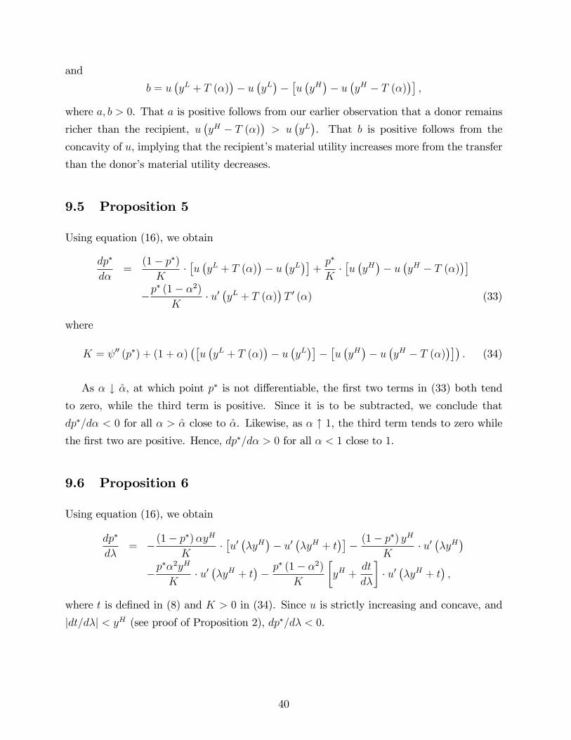
and
b = u(yL + T (α)
)− u
(yL)−[u(yH)− u
(yH − T (α)
)],
where a, b > 0. That a is positive follows from our earlier observation that a donor remains
richer than the recipient, u(yH − T (α)
)> u
(yL). That b is positive follows from the
concavity of u, implying that the recipient’s material utility increases more from the transfer
than the donor’s material utility decreases.
9.5 Proposition 5
Using equation (16), we obtain
dp∗
dα=
(1− p∗)K
·[u(yL + T (α)
)− u
(yL)]
+p∗
K·[u(yH)− u
(yH − T (α)
)]−p∗ (1− α2)
K· u′(yL + T (α)
)T ′ (α) (33)
where
K = ψ′′ (p∗) + (1 + α)([u(yL + T (α)
)− u
(yL)]−[u(yH)− u
(yH − T (α)
)]). (34)
As α ↓ α, at which point p∗ is not differentiable, the first two terms in (33) both tendto zero, while the third term is positive. Since it is to be subtracted, we conclude that
dp∗/dα < 0 for all α > α close to α. Likewise, as α ↑ 1, the third term tends to zero while
the first two are positive. Hence, dp∗/dα > 0 for all α < 1 close to 1.
9.6 Proposition 6
Using equation (16), we obtain
dp∗
dλ= −(1− p∗)αyH
K·[u′(λyH
)− u′
(λyH + t
)]− (1− p∗) yH
K· u′(λyH
)−p∗α2yH
K· u′(λyH + t
)− p∗ (1− α2)
K
[yH +
dt
dλ
]· u′(λyH + t
),
where t is defined in (8) and K > 0 in (34). Since u is strictly increasing and concave, and
|dt/dλ| < yH (see proof of Proposition 2), dp∗/dλ < 0.
40
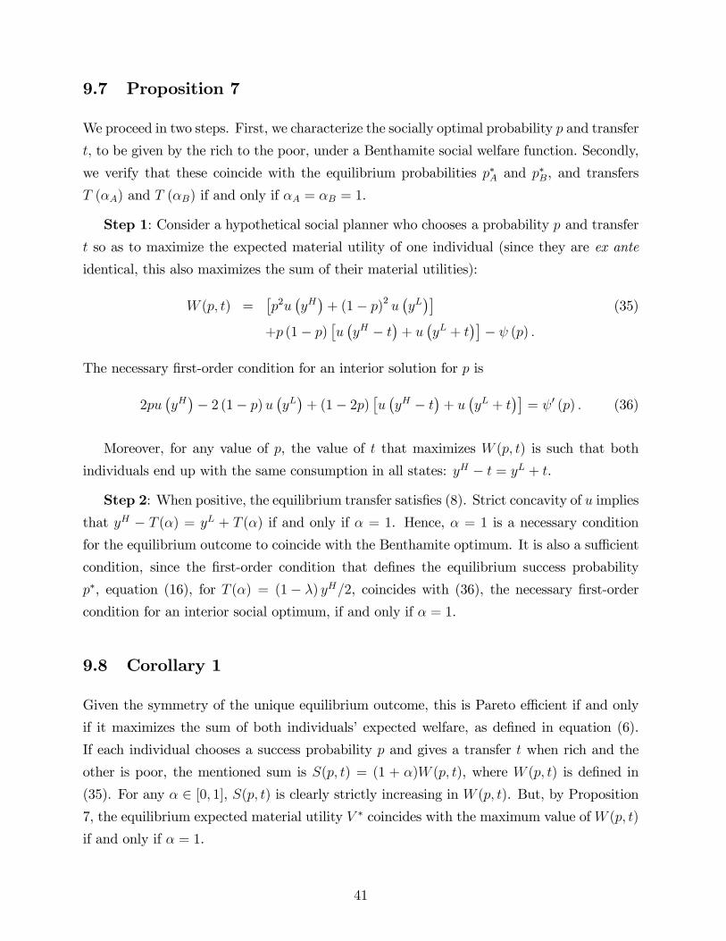
9.7 Proposition 7
We proceed in two steps. First, we characterize the socially optimal probability p and transfer
t, to be given by the rich to the poor, under a Benthamite social welfare function. Secondly,
we verify that these coincide with the equilibrium probabilities p∗A and p∗B, and transfers
T (αA) and T (αB) if and only if αA = αB = 1.
Step 1: Consider a hypothetical social planner who chooses a probability p and transfer
t so as to maximize the expected material utility of one individual (since they are ex ante
identical, this also maximizes the sum of their material utilities):
W (p, t) =[p2u
(yH)
+ (1− p)2 u(yL)]
(35)
+p (1− p)[u(yH − t
)+ u
(yL + t
)]− ψ (p) .
The necessary first-order condition for an interior solution for p is
2pu(yH)− 2 (1− p)u
(yL)
+ (1− 2p)[u(yH − t
)+ u
(yL + t
)]= ψ′ (p) . (36)
Moreover, for any value of p, the value of t that maximizes W (p, t) is such that both
individuals end up with the same consumption in all states: yH − t = yL + t.
Step 2: When positive, the equilibrium transfer satisfies (8). Strict concavity of u implies
that yH − T (α) = yL + T (α) if and only if α = 1. Hence, α = 1 is a necessary condition
for the equilibrium outcome to coincide with the Benthamite optimum. It is also a suffi cient
condition, since the first-order condition that defines the equilibrium success probability
p∗, equation (16), for T (α) = (1− λ) yH/2, coincides with (36), the necessary first-order
condition for an interior social optimum, if and only if α = 1.
9.8 Corollary 1
Given the symmetry of the unique equilibrium outcome, this is Pareto effi cient if and only
if it maximizes the sum of both individuals’expected welfare, as defined in equation (6).
If each individual chooses a success probability p and gives a transfer t when rich and the
other is poor, the mentioned sum is S(p, t) = (1 + α)W (p, t), where W (p, t) is defined in
(35). For any α ∈ [0, 1], S(p, t) is clearly strictly increasing in W (p, t). But, by Proposition
7, the equilibrium expected material utility V ∗ coincides with the maximum value ofW (p, t)
if and only if α = 1.
41
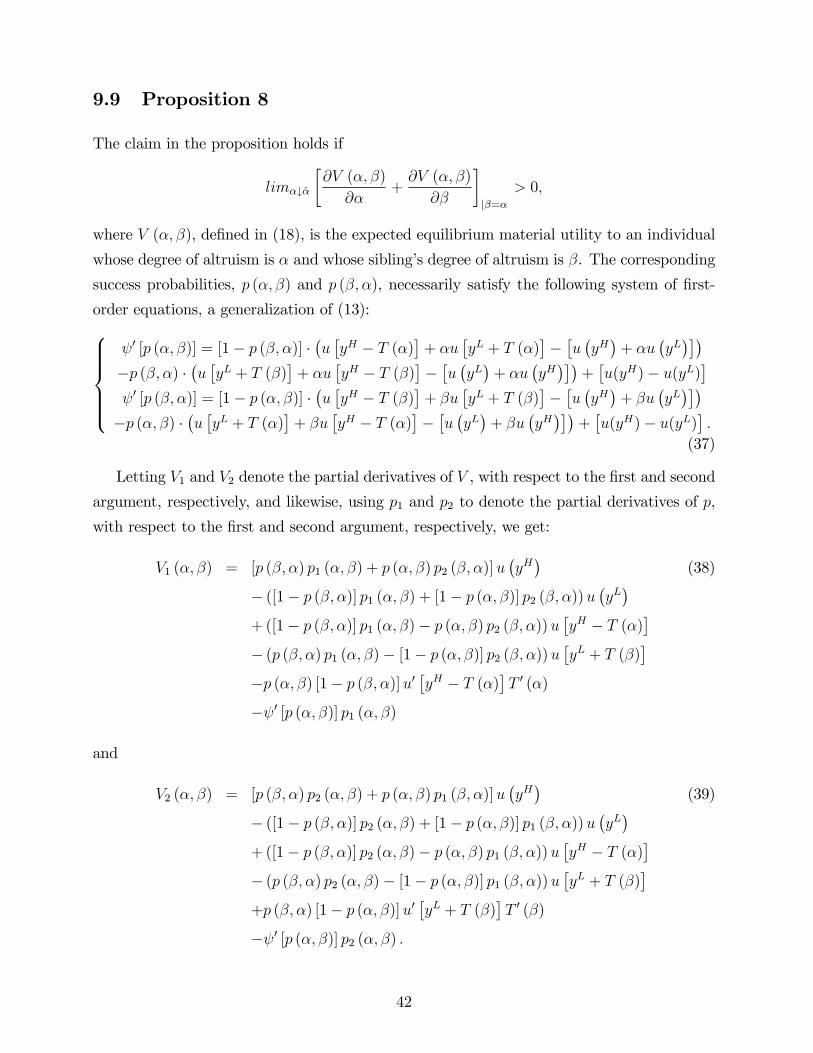
9.9 Proposition 8
The claim in the proposition holds if
limα↓α
[∂V (α, β)
∂α+∂V (α, β)
∂β
]|β=α
> 0,
where V (α, β), defined in (18), is the expected equilibrium material utility to an individual
whose degree of altruism is α and whose sibling’s degree of altruism is β. The corresponding
success probabilities, p (α, β) and p (β, α), necessarily satisfy the following system of first-
order equations, a generalization of (13):ψ′ [p (α, β)] = [1− p (β, α)] ·
(u[yH − T (α)
]+ αu
[yL + T (α)
]−[u(yH)
+ αu(yL)])
−p (β, α) ·(u[yL + T (β)
]+ αu
[yH − T (β)
]−[u(yL)
+ αu(yH)])
+[u(yH)− u(yL)
]ψ′ [p (β, α)] = [1− p (α, β)] ·
(u[yH − T (β)
]+ βu
[yL + T (β)
]−[u(yH)
+ βu(yL)])
−p (α, β) ·(u[yL + T (α)
]+ βu
[yH − T (α)
]−[u(yL)
+ βu(yH)])
+[u(yH)− u(yL)
].
(37)
Letting V1 and V2 denote the partial derivatives of V , with respect to the first and second
argument, respectively, and likewise, using p1 and p2 to denote the partial derivatives of p,
with respect to the first and second argument, respectively, we get:
V1 (α, β) = [p (β, α) p1 (α, β) + p (α, β) p2 (β, α)]u(yH)
(38)
− ([1− p (β, α)] p1 (α, β) + [1− p (α, β)] p2 (β, α))u(yL)
+ ([1− p (β, α)] p1 (α, β)− p (α, β) p2 (β, α))u[yH − T (α)
]− (p (β, α) p1 (α, β)− [1− p (α, β)] p2 (β, α))u
[yL + T (β)
]−p (α, β) [1− p (β, α)]u′
[yH − T (α)
]T ′ (α)
−ψ′ [p (α, β)] p1 (α, β)
and
V2 (α, β) = [p (β, α) p2 (α, β) + p (α, β) p1 (β, α)]u(yH)
(39)
− ([1− p (β, α)] p2 (α, β) + [1− p (α, β)] p1 (β, α))u(yL)
+ ([1− p (β, α)] p2 (α, β)− p (α, β) p1 (β, α))u[yH − T (α)
]− (p (β, α) p2 (α, β)− [1− p (α, β)] p1 (β, α))u
[yL + T (β)
]+p (β, α) [1− p (α, β)]u′
[yL + T (β)
]T ′ (β)
−ψ′ [p (α, β)] p2 (α, β) .
42
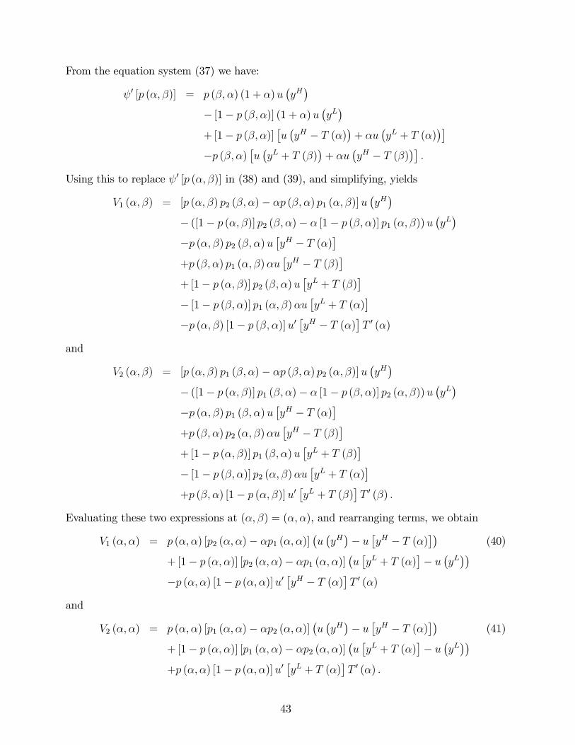
From the equation system (37) we have:
ψ′ [p (α, β)] = p (β, α) (1 + α)u(yH)
− [1− p (β, α)] (1 + α)u(yL)
+ [1− p (β, α)][u(yH − T (α)
)+ αu
(yL + T (α)
)]−p (β, α)
[u(yL + T (β)
)+ αu
(yH − T (β)
)].
Using this to replace ψ′ [p (α, β)] in (38) and (39), and simplifying, yields
V1 (α, β) = [p (α, β) p2 (β, α)− αp (β, α) p1 (α, β)]u(yH)
− ([1− p (α, β)] p2 (β, α)− α [1− p (β, α)] p1 (α, β))u(yL)
−p (α, β) p2 (β, α)u[yH − T (α)
]+p (β, α) p1 (α, β)αu
[yH − T (β)
]+ [1− p (α, β)] p2 (β, α)u
[yL + T (β)
]− [1− p (β, α)] p1 (α, β)αu
[yL + T (α)
]−p (α, β) [1− p (β, α)]u′
[yH − T (α)
]T ′ (α)
and
V2 (α, β) = [p (α, β) p1 (β, α)− αp (β, α) p2 (α, β)]u(yH)
− ([1− p (α, β)] p1 (β, α)− α [1− p (β, α)] p2 (α, β))u(yL)
−p (α, β) p1 (β, α)u[yH − T (α)
]+p (β, α) p2 (α, β)αu
[yH − T (β)
]+ [1− p (α, β)] p1 (β, α)u
[yL + T (β)
]− [1− p (β, α)] p2 (α, β)αu
[yL + T (α)
]+p (β, α) [1− p (α, β)]u′
[yL + T (β)
]T ′ (β) .
Evaluating these two expressions at (α, β) = (α, α), and rearranging terms, we obtain
V1 (α, α) = p (α, α) [p2 (α, α)− αp1 (α, α)](u(yH)− u
[yH − T (α)
])(40)
+ [1− p (α, α)] [p2 (α, α)− αp1 (α, α)](u[yL + T (α)
]− u
(yL))
−p (α, α) [1− p (α, α)]u′[yH − T (α)
]T ′ (α)
and
V2 (α, α) = p (α, α) [p1 (α, α)− αp2 (α, α)](u(yH)− u
[yH − T (α)
])(41)
+ [1− p (α, α)] [p1 (α, α)− αp2 (α, α)](u[yL + T (α)
]− u
(yL))
+p (α, α) [1− p (α, α)]u′[yL + T (α)
]T ′ (α) .
43
Finally, using the first-order equation (8) that defines T (α) for α > α, and rearranging
terms, we get:
V1 (α, α) + V2 (α, α) = (1− α) [p1 (α, α) + p2 (α, α)] · p (α, α)[u(yH)− u
(yH − T (α)
)](1− α) [p1 (α, α) + p2 (α, α)] · [1− p (α, α)]
[u(yL + T (α)
)− u
(yL)]
+p (α, α) [1− p (α, α)] (1− α)u′(yL + T (α)
)T ′ (α) .
This tends to a positive number as α tends to α from above, since the first two terms then
tend to zero while the last term tends to a positive number.
9.10 Lemma 1
Using the expressions in (40) and (41) for the partial derivatives V1 and V2, we obtain from
(20):
D (α) =
[V1(α, α) +
1
2V2(α, α)
]= p (α, α) [1− p (α, α)]
[1
2u′[yL + T (α)
]− u′
[yH − T (α)
]]T ′ (α)
+
[(1
2− α
)p1 (α, α) +
(1− α
2
)p2 (α, α)
]·
·[p (α, α)
(u(yH)− u
[yH − T (α)
])+ [1− p (α, α)]
(u[yL + T (α)
]− u
(yL))]
=
(1
2− α
)· p (α, α) [1− p (α, α)]u′
[yL + T (α)
]T ′ (α)
+
[(1
2− α
)p1 (α, α) +
(1− α
2
)p2 (α, α)
]·
·[p (α, α)
(u(yH)− u
[yH − T (α)
])+ [1− p (α, α)]
(u[yL + T (α)
]− u
(yL))]
.
9.11 Proposition 10
The result follows from Proposition 9, together with the observation that, for any α < α,
D (α) = 0 (simply set T (α) = T ′ (α) = 0 in (21)).
9.12 Proposition 11
Recall that T (α) = 0 for all α ≤ α, and that T (α) tends to zero as α ↓ α. Recall also thatp1 > 0 and p2 < 0 for all α > α, see Proposition 3. The drift function D being continuous
44
at each α ∈ A, we obtain, by applying the definition of local evolutionary stability inProposition 9:
1. Suppose that λ ≥ 1yH
(u′)−1 [2u′ (yH)], so that α ≥ 1/2: then there exists no locally
evolutionarily robust degree of altruism, since D (α) = 0 for any α < α, and α > α ≥1/2 ⇒ D (α) < 0.
2. Suppose that λ < 1yH
(u′)−1 [2u′ (yH)], so that α < 1/2: then if there exists a locally
evolutionarily robust degree of altruism α ∈ A, it must be that α ∈ (α, 1/2), since
limα↓αD (α) > 0 (because G (α), i.e., the very last term in the expression for D above,
tends to 0 as α ↓ α), and D (1/2) < 0.
9.13 Corollary 2
Assume that λ < λ (so that α < 1/2) and that the success probabilities are exogenously
fixed and equal: pA = pB = p ∈ (0, 1). For every α ∈ int (A), we then have
D (α) = p (1− p) ·[
1
2u′[yL + T (α)
]− u′
[yH − T (α)
]]T ′ (α) . (42)
Since T ′ (α) = 0 for all α < α, by Proposition 9 no α ≤ α is locally evolutionarily stable.
Turning now to α > α, T ′ (α) > 0 for all α > α and T (α) satisfies the first-order condition
(8). Hence, for every α ∈ int (A) exceeding α:
D (α) = p (1− p) ·(
1
2− α
)u′[yL + T (α)
]T ′ (α) .
By Proposition 9, this implies that α is locally evolutionarily stable if and only if α = 1/2.
From (18) we obtain that A = α ∈ [0, 1] : α 6= α. In particular, (α, 1) ⊂ int (A). Hence,
α = 1/2 is the only locally stable degree of altruism.
9.14 Proposition 12
Recall the following properties:
• for all α ≤ α: T (α) = 0, and hence F (α) = G (α) = 0
• for all α > α: T (α) > 0 and T ′ (α) > 0, and hence F (α) > 0 and G (α) > 0
45
• for all α > α: p1 > 0 and p2 < 0 (see Proposition 3)
• p1 + p2 > 0 for α slightly below 1 (see Proposition 5).
The drift function D being continuous at each α ∈ A, we obtain, by applying the defini-tion of local evolutionary stability in Proposition 9:
1. There exists no locally evolutionarily robust degree of altruism α < α, since D (α) = 0
for all α < α.
2. Assume now that κ < 1, and consider the two cases:
(a) α > 1+κ2: then there exists no locally evolutionarily robust degree of altruism,
since α > α ≥ 1+κ2⇒ D (α) < 0.
(b) α < 1+κ2: then if there exists a locally evolutionarily robust degree of altruism
α ∈ A, then it must be that α ∈(α, 1+κ
2
), since limα↓αD (α) > 0 (because G (α)
tends to 0 as α ↓ α), and D(
1+κ2
)< 0.
3. Assume now that κ = 1. Then D (α) = (1− α) [F (α) + (p1 (α, α) + p2 (α, α)) ·G (α)].
The properties recalled above imply that D (α) = 0 if α = 1, and that D (α) > 0 for α
close to 1.
4. An increase in κ leads to an upward shift in D (α) for all α ∈ (α, 1). Hence, if there
exists a locally evolutionarily robust degree of altruism α ∈ (α, 1), then it is strictly
increasing in κ.
46
References
Alesina A. and P. Giuliano (2007): “The Power of the Family,”NBER WP 13051.
Alger I. and J.W. Weibull (2007): “The Fetters of the Sib: Weber Meets Darwin,”
Stockholm School of Economics Working Paper 682.
Alger I. and J.W. Weibull (2008): “Family Ties, Incentives and Development: A Model of
Coerced Altruism,”in Basu, K., and R. Kanbur, eds., Arguments for a Better World: Essays
in Honor of Amartya Sen, Volume II: Society, Institutions and Development, Oxford: Oxford
University Press.
Altonji, J.G., F. Hayashi and L. Kotlikoff (1997): “Parental Altruism and Inter Vivos
Transfers: Theory and Evidence,”Journal of Political Economy, 105:1121-1166.
Arnott R. and J. Stiglitz (1991): “Moral Hazard and Nonmarket Institutions: Dysfunc-
tional Crowding Out of Peer Monitoring?”American Economic Review, 81:179-190.
Azam J.P. and F. Gubert (2005): “Those in Kayes. The Impact of Remittances on their
Recipients in Africa,”Revue Economique, 56:1331-1358.
Banfield E. (1958): The Moral Basis of a Backward Society. Chicago: Free Press.
Bartle R. (1976): The Elements of Real Analysis, Second Edition. New York: John Wiley
and Sons.
Becker G.S. (1974): “A Theory of Social Interactions,” Journal of Political Economy,
82:1063-1093.
Bergstrom, T.C. (1995): “On the Evolution of Altruistic Ethical Rules for Siblings,”
American Economic Review, 85:58-81.
Bergstrom, T.C. (2003): “The Algebra of Assortative Encounters and the Evolution of
Cooperation,”International Game Theory Review, 5:211-228.
Bisin, A., and T. Verdier (2001): “The Economics of Cultural Transmission and the
Dynamics of Preferences,”Journal of Economic Theory, 97:298-319.
Bisin, A., G. Topa, and T. Verdier (2004): “Cooperation as a Transmitted Cultural
Trait,”Rationality and Society, 16:477-507.
Bowles, S. (2009): “DidWarfare Among Ancestral Hunter-Gatherers Affect the Evolution
of Human Social Behaviors?”Science, 324:1293 - 1298.
47
Bramoullé Y. and R. Kranton (2007): “Risk-Sharing Networks,” Journal of Economic
Behavior and Organization, 64:275-294.
Bruce N. and M. Waldman (1990): “The Rotten-Kid Theorem Meets the Samaritan’s
Dilemma,”Quarterly Journal of Economics, 105:155-165.
Cavalli-Sforza, L. L. and M. W. Feldman (1981): Cultural Transmission and Evolution:
A Quantitative Approach, Princeton, N.J.: Princeton University Press.
Chami, R. (1998): “Private Income Transfers andMarket Incentives,”Economica, 65:557-
580.
Chen, Z. and F. Woolley (2001): “A Cournot-Nash Model of Family Decision Making,”
Economic Journal, 111:722-748.
Coate, S. (1995): “Altruism, the Samaritan’s Dilemma, and Government Transfer Pol-
icy,”American Economic Review, 85:46-57.
Coate, S. and M. Ravallion (1993): “Reciprocity without Commitment: Characterization
and Performance of Informal Insurance Arrangements,”Journal of Development Economics,
40:1-24.
Cox, D. and M. Fafchamps (2008): “Extended Family and Kinship Networks: Economic
Insights and Evolutionary Directions,” in T. Schultz T. and J. Strauss, eds., Handbook of
Development Economics, 4. Amsterdam: North-Holland.
Cox, D., E. Galasso and E. Jimenez (2006): “Private Transfers in a Cross Section of
Developing Countries,”CRR WP 2006-2.
Cox, D., B.E. Hansen and E. Jimenez(2004): “How Responsive are Private Transfers to
Income? Evidence from a Laissez-Faire Economy," Journal of Public Economics, 88:2193-
2219.
Edgeworth, F.Y. (1881): Mathematical Psychics: An Essay on the Application of Math-
ematics to the Moral Sciences. London: Kegan Paul.
Eshel, I. and A. Shaked (2001): “Partnership,”Journal of Theoretical Biology, 208:457-
474.
Fafchamps, M. and S. Lund (2003): "Risk-Sharing Networks in Rural Philippines," Jour-
nal of Development Economics, 71:261-287.
48
Fernandes, A. (2008): “Altruism, Labor Supply and Redistributive Neutrality,” forth-
coming, Journal of Population Economics.
Foster, A. and M.R. Rosenzweig (2001): “Imperfect Commitment, Altruism and the Fam-
ily: Evidence from Transfer Behaviour in Low-Income Rural Areas,”Review of Economics
and Statistics, 83: 389-407.
Gatti, R. (2005): “Family Altruism and Incentives,”Scandinavian Journal of Economics,
107:67-81.
Genicot, G. and D. Ray (2003): “Group Formation in Risk-Sharing Arrangements,”
Review of Economic Studies, 70:87-113.
Gonzales, A. (1998): A Comparative Study of Family Values and Structures among Mex-
ican Americans and Non-Hispanic Whites. Doctoral Dissertation, The University of Texas
at Austin.
Grafen, A. (2006): “Optimization of Inclusive Fitness,”Journal of Theoretical Biology,
238:541—563.
Güth, W. and B. Peleg (2001): “When Will Payoff Maximization Survive? An Indirect
Evolutionary Analysis,”Journal of Evolutionary Economics, 11:479-499.
Hajnal, J. (1982): “Two Kinds of Preindustrial Household Formation,”Population and
Development Review, 8:449-494.
Haldane, J.B.S. (1955): “Population Genetics,”New Biology, 18:34-51.
Hamilton, W.D. (1964a): “The Genetical Evolution of Social Behaviour. I,”Journal of
Theoretical Biology, 7:1-16.
Hamilton, W.D. (1964b): “The Genetical Evolution of Social Behaviour. II,”Journal of
Theoretical Biology, 7:17-52.
Hauk E. and M. Saez-Martí (2002): “On the Cultural Transmission of Corruption,”
Journal of Economic Theory, 107:311-335.
Heifetz, A., C. Shannon and Y. Spiegel (2007): “The Dynamic Evolution of Preferences,”
Economic Theory, 32:251-286.
Hwang, S.-H. and S. Bowles (2009): “Is Altruism Bad for Cooperation?”mimeo, Univer-
sity of Massachusetts at Amherst and Santa Fe Institute.
49
Keefe, S.E, A.M. Padilla and M.L. Carlos (1979): “The Mexican American Extended
Family as an Emotional Support System,”Human Organization, 38:144-152.
Kohler, H.-P. and E.A. Hammel (2001): “On the Role of Families and Kinship Networks
in Pre-Industrial Agricultural Societies: An Analysis of the 1698 Slovenian Census,”Journal
of Population Economics, 14:21-49.
Kolm, S.-C. and J.M Ythier, eds. (2006): Handbook of Reciprocity, Giving and Altruism.
Amsterdam: North-Holland.
Kussmaul, A., (1981): Servants in Husbandry in Early Modern England, Cambridge:
Cambridge University Press.
Laferrère, A. and F.-C. Wolff (2006): “Microeconomic Models of Family Transfers,”
in Kolm, S.-C., and J.M Ythier, eds., Handbook of Reciprocity, Giving and Altruism 2.
Amsterdam: North-Holland.
Lindbeck, A. and S. Nyberg (2006): “Raising Children to Work Hard: Altruism, Work
Norms and Social Insurance,”Quarterly Journal of Economics, 121:1473-1503.
Lindbeck, A. and J.W. Weibull (1988): “Altruism and Time Consistency: The Economics
of Fait Accompli,”Journal of Political Economy, 96:1165-1182.
Macfarlane, A. (1978): The Origins of English Individualism. Oxford: Basil Blackwell.
Macfarlane, A. (1992): “On Individualism,”Proceedings of the British Academy, 82:171-
199.
Maitra, P. and R. Ray (2003): “The Effect of Transfers on Household Expenditure Pat-
terns and Poverty in South Africa,”Journal of Development Economics, 71:23-49.
Manacorda, M. and E. Moretti (2006): “Why Do Most Italian Youths Live with Their
Parents? Intergenerational Transfers and Household Structure,” Journal of the European
Economic Assocation, 4:800-829.
Miller, D. and A.L. Paulson (1999): “Informal Insurance and Moral Hazard: Gambling
and Remittances in Thailand,”mimeo, Princeton and Northwestern.
Montesquieu, C.-L. (1748): De l’esprit des lois. Genève: Barrillot & Fils.
Ozment, S. (1975): The Reformation in the Cities: The Appeal of Protestantism to
Sixteenth-Century Germany and Switzerland. New Haven: Yale University Press.
Ozment, S. (1992): Protestants: The Birth of a Revolution. New York: Doubleday.
50
Rosenzweig, M.R. and K. Wolpin (1993): “Intergenerational Support and the Life-Cycle
Incomes of Young Men and Their Parents: Human Capital Investments, Coresidence, and
Intergenerational Financial Transfers,”Journal of Labor Economics, 11:84-112.
Rowthorn, R. (2006): “The Evolution of Altruism between Siblings: Hamilton’s Rule
Revisited,”Journal of Theoretical Biology, 241:774—790.
Sethi, R. and E. Somanathan (2001): “Preference Evolution and Reciprocity,”Journal
of Economic Theory, 97:273-297.
Sober, E. and D.S. Wilson (1998): Unto Others. Cambridge: Harvard University Press.
Tabellini, G. (2008a): “Institutions and Culture,” Journal of the European Economic
Association, 6:255—294.
Tabellini, G. (2008b): “The Scope of Cooperation: Values and Incentives,”Quarterly
Journal of Economics, 123:905-950.
Townsend, R. (1994): “Risk and Insurance in Village India," Econometrica, 62:539-591.
Trivers, R.L. (1971): “The Evolution of Reciprocal Altruism," Quarterly Review of Bi-
ology, 46:35-57.
Udry, C. (1990): “Rural Credit in Northern Nigeria: Credit as Insurance in a Rural
Economy,”World Bank Economic Review, 4:251-269.
Weber, M. (1951): The Religion of China. Glencoe: The Free Press.
Wilson, D.S. and E.O. Wilson (2007): “Rethinking the Theoretical Foundation of Socio-
biology,”Quarterly Review of Biology, 82:327-348.
Wright, S. (1921): “Systems of Mating,”Genetics, 6:111-178.
Wright, S. (1922): “Coeffi cients of Inbreeding and Relationship,”American Naturalist,
56:330-338.
51
![[hal-00435431, v1] Kinship, Incentives and Evolution · 2017-05-05 · KINSHIP, INCENTIV ES AND EVOLUTION ... 24 Nov 2009. Kinship, Incentives and Evolution Ingela Alger Jörgen W](https://img.pdfslide.net/doc/110x75/5f778aa0bddbbf684727a5cb/hal-00435431-v1-kinship-incentives-and-evolution-2017-05-05-kinship-incentiv.jpg)