Embed Size (px)
Citation preview
HAL Id: hal-02325059https://hal.archives-ouvertes.fr/hal-02325059
Submitted on 22 Oct 2019
HAL is a multi-disciplinary open accessarchive for the deposit and dissemination of sci-entific research documents, whether they are pub-lished or not. The documents may come fromteaching and research institutions in France orabroad, or from public or private research centers.
L’archive ouverte pluridisciplinaire HAL, estdestinée au dépôt et à la diffusion de documentsscientifiques de niveau recherche, publiés ou non,émanant des établissements d’enseignement et derecherche français ou étrangers, des laboratoirespublics ou privés.
Landau level broadening, hyperuniformity, and discretescale invariance
Jean-Noël Fuchs, Rémy Mosseri, Julien Vidal
To cite this version:Jean-Noël Fuchs, Rémy Mosseri, Julien Vidal. Landau level broadening, hyperuniformity, and discretescale invariance. Physical Review B: Condensed Matter and Materials Physics (1998-2015), AmericanPhysical Society, 2019, 100 (12), �10.1103/PhysRevB.100.125118�. �hal-02325059�
PHYSICAL REVIEW B 100, 125118 (2019)
Landau level broadening, hyperuniformity, and discrete scale invariance
Jean-Noël Fuchs ,* Rémy Mosseri,† and Julien Vidal ‡
Sorbonne Université, CNRS, Laboratoire de Physique Théorique de la Matière Condensée, LPTMC, F-75005 Paris, France
(Received 19 March 2019; revised manuscript received 22 August 2019; published 9 September 2019)
We study the energy spectrum of a two-dimensional electron in the presence of both a perpendicular magneticfield and a potential. In the limit where the potential is small compared to the Landau level spacing, we showthat the broadening of Landau levels is simply expressed in terms of the structure factor of the potential. Forpotentials that are either periodic or random, we recover known results. Interestingly, for potentials with a denseFourier spectrum made of Bragg peaks (as found, e.g., in quasicrystals), we find an algebraic broadening withthe magnetic field characterized by the hyperuniformity exponent of the potential. Furthermore, if the potentialis self-similar such that its structure factor has a discrete scale invariance, the broadening displays log-periodicoscillations together with an algebraic envelope.
DOI: 10.1103/PhysRevB.100.125118
I. INTRODUCTION
In the presence of a magnetic field, the energy spectrumof noninteracting electrons in two dimensions is known toconsist of Landau levels. These discrete energy levels areresponsible for many remarkable phenomena, among which isthe celebrated integer quantum Hall effect [1,2]. Each Landaulevel has a macroscopic degeneracy that is proportional to thestrength of the magnetic field. This degeneracy is expectedto be lifted by a generic perturbation leading to a broadeningof Landau levels that may have important physical conse-quences. For instance, plateaus observed in the Hall resistanceare directly related to the broadening induced by disorder, asrealized early by Ando et al. [3–5]. Most studies on Landaulevel broadening focused on disordered systems (see Ref. [6]for a review), but the role played by periodic potentials hasalso attracted much attention following the original work ofRauh [7,8]. Based on a free-electron picture, Rauh’s approachalso allows one to qualitatively understand the Landau levelbroadening in the small-field limit of the Hofstadter butterflyfor periodic lattices [9,10], although a quantitative analysis re-quires a semiclassical treatment [11]. Recently, the Hofstadterbutterfly of some quasiperiodic systems has been investigated,unveiling an unusual broadening of Landau levels [12] differ-ent from the one expected for periodic or disordered systems,hence suggesting a nontrivial mechanism for potentials with adense set of Bragg peaks.
The goal of the present paper is to provide a generalframework to compute the broadening of Landau levels inthe presence of an arbitrary potential. Our main result, givenin Eq. (11), relates the variance of the lowest Landau level(LLL) to the structure factor of the perturbing potential (anextension to higher-energy Landau levels is straightforward).
*[email protected]†[email protected]‡[email protected]
This simple expression reproduces the aforementioned resultsfor disordered and periodic cases, but it also allows us toinvestigate more subtle potentials (see Fig. 1 for a summaryof the results). In particular, we find that when the Fourierspectrum of the potential is dense and made of Bragg peaks(as in quasicrystals), the variance of the LLL increases al-gebraically with the magnetic field [see Eq. (22)] with anexponent characterizing the hyperuniformity of the potential.This notion of hyperuniformity is commonly used to describesets of points with an unusually large suppression of densityfluctuations at long wavelengths [13]. We also show that ifthe potential has a discrete scale invariance [14,15], thenthe variance displays log-periodic oscillations together with apower-law envelope. To illustrate these results, we considerthree examples of quasiperiodic potentials, for which wecompute exactly the hyperuniformity exponent and the periodof these oscillations, when it exists.
Vari
ance
ofth
eLLL
Magnetic field0
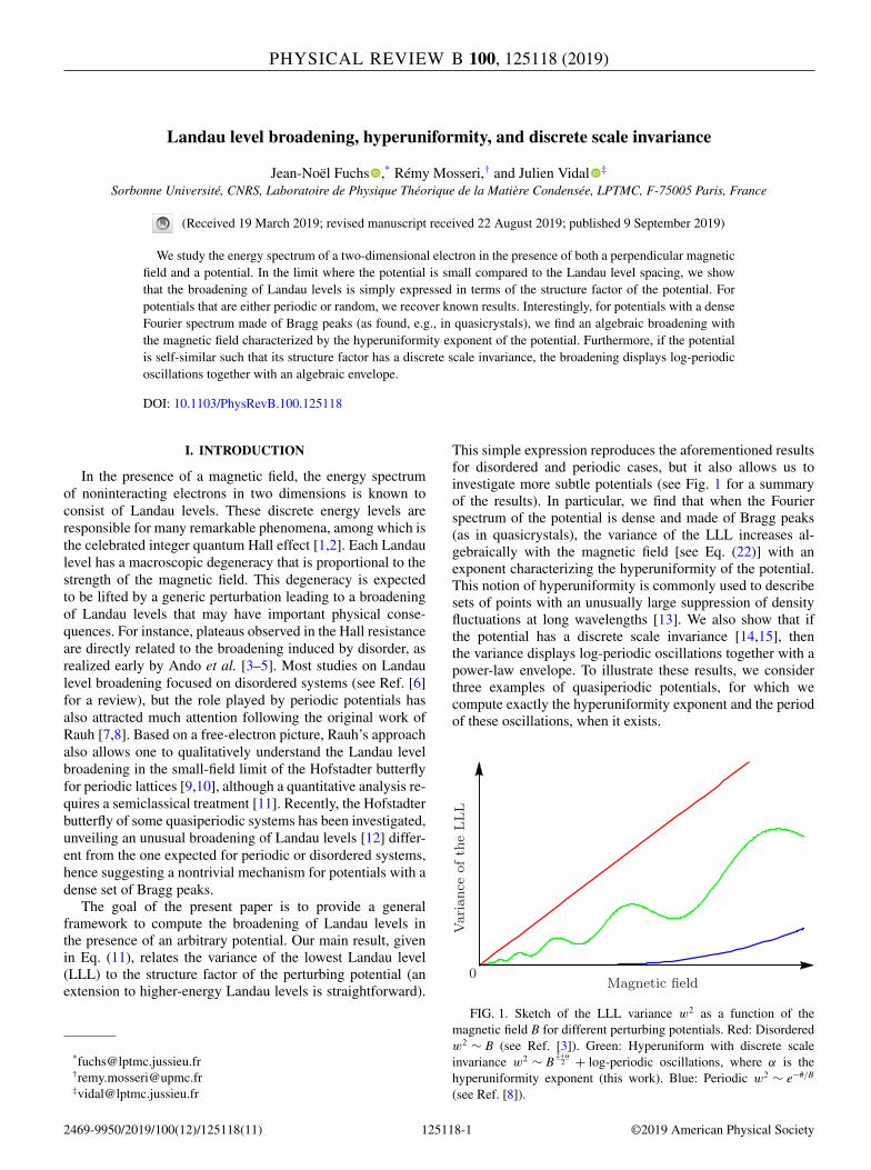
FIG. 1. Sketch of the LLL variance w2 as a function of themagnetic field B for different perturbing potentials. Red: Disorderedw2 ∼ B (see Ref. [3]). Green: Hyperuniform with discrete scaleinvariance w2 ∼ B
2+α2 + log-periodic oscillations, where α is the
hyperuniformity exponent (this work). Blue: Periodic w2 ∼ e−#/B
(see Ref. [8]).
2469-9950/2019/100(12)/125118(11) 125118-1 ©2019 American Physical Society
FUCHS, MOSSERI, AND VIDAL PHYSICAL REVIEW B 100, 125118 (2019)
II. LANDAU LEVELS PERTURBED BY A POTENTIAL
To begin with, let us recall a few well-known results. TheHamiltonian describing a particle of mass m and charge e in amagnetic field B = ∇ × A is given by
H0 = (p − eA)2
2m. (1)
Here, we consider a two-dimensional system with a magneticfield perpendicular to the plane. Such a field can be describedby the symmetric gauge where the vector potential readsA = B(−y/2, x/2, 0). The spectrum of H0 consists in equidis-tant energy levels known as Landau levels,
En = hωc(n + 1/2), ∀n ∈ N, (2)
where ωc = |eB|/m is the cyclotron frequency. Each Landaulevel has a degeneracy proportional to the sample area A andthe magnetic field. In the following, we set h = e = 1.
Our aim is to study the behavior of the Landau levels in thepresence of a time-independent potential. Thus, we considerthe following general Hamiltonian:
H = H0 + V (x, y), (3)
and we assume that the magnitude of the potential is smallcompared to the Landau level spacing ωc � |V |. In thisregime, we can neglect the coupling between different Landaulevels and use degenerate perturbation theory to computethe degeneracy splitting of a single level. Without loss ofgenerality, we assume V (x, y) � 0 and B > 0 in the following.
III. VARIANCE OF THE LLL
For simplicity, in the following we focus on the LLLcorresponding to n = 0 for which the nonperturbed wavefunctions, in the thermodynamic limit, can be chosen as
ϕl (z) = 〈x, y|l〉 = 1√2π l2
B l! 2lzl e−|z|2/4, (4)
where z = (x + iy)/lB, l = 0, 1, . . . , Nφ − 1 is the angularmomentum, Nφ = A/(2π l2
B) � 1 is the degeneracy of theLLL, and lB = 1/
√B is the magnetic length.
To characterize the broadening of the LLL due to thepotential, we consider its variance defined by
w2 = 1
Nφ
Nφ−1∑p=0
ε2p −
⎛⎝ 1
Nφ
Nφ−1∑p=0
εp
⎞⎠
2
, (5)
where εp’s are eigenenergies of H projected onto the LLL.This variance can be recast as
w2 = 1
Nφ
Nφ−1∑l=0
Nφ−1∑l ′=0
|〈l|V |l ′〉|2 −⎛⎝ 1
Nφ
Nφ−1∑l=0
〈l|V |l〉⎞⎠
2
, (6)
so that one does not need to compute explicitly the εp’s.Setting r = (x, y) = r(cos θ, sin θ ), a matrix element of theperturbation potential in the LLL basis {|l〉, l = 0, . . . ,
Nφ − 1} reads
〈l|V |l ′〉 =∫
dq(2π )2
V (q)
2π√
l! l ′! 2l+l ′
×∫ ∞
0
dr
lB
(r
lB
)1+l+l ′
e− r2
2l2B
∫ 2π
0dθ eiq·reiθ (l−l ′ ),
(7)
where we introduced the Fourier transform of the potential
V (q) =∫
dr e−iq·rV (r). (8)
In the large-Nφ (thermodynamical) limit, one then gets
∞∑l=0
〈l|V |l〉 = V (0)
2π l2B
, (9)
∞∑l=0
∞∑l ′=0
|〈l|V |l ′〉|2 = 1
2π l2B
∫dq
(2π )2|V (q)|2e−|q|2l2
B/2. (10)
Finally, one obtains the following expression for the variance:
w2 =∫
dq(2π )2
S(q)e−|q|2l2B/2, (11)
where we introduced the structure factor
S(q) = |V (q)|2A (1 − δq,0). (12)
Note that the term proportional to δq,0 comes from the secondterm of Eq. (5) and is irrelevant only if V (0) = 0. The varianceis therefore essentially equal to the integral of the structurefactor over a disk of radius l−1
B , which is the main result ofthis paper. Before discussing the most interesting case of apotential with a dense Fourier spectrum, let us first show thatthis expression allows one to recover known results for simplepotentials.
IV. PERIODIC POTENTIAL
For a periodic potential of strength V0 with a single spatialfrequency a−1,
V (x, y) = V0[cos(2πx/a) + cos(2πy/a)], (13)
Eq. (11) leads to
w2 = V 20 e− 2π2
Ba2 , (14)
in agreement with the expression found by Rauh [8] (seeAppendix A for details). The generalization to Fourier spectrawith a finite set of frequencies is straightforward, even if thepotential is no longer periodic. In the zero-field limit, theLLL broadening is exponential and controlled by the smallestfrequency. The case of a dense set of frequencies is moresubtle.
V. RANDOM POTENTIAL
Landau level broadening due to an uncorrelated randompotential has been widely studied in the literature [6]. For the
125118-2
LANDAU LEVEL BROADENING, HYPERUNIFORMITY, AND … PHYSICAL REVIEW B 100, 125118 (2019)
simple case of a random potential with zero mean and white-noise correlations,
V (r) = 0, (15)
V (r)V (r′) = (V0 a)2δ(r − r′), (16)
where the overline denotes the average over disorder realiza-tions, Eq. (11) gives
w2 = V 20
a2
2π l2B
= V 20
Ba2
2π, (17)
in agreement with the result of Ando [5] (see Appendix B fordetails). This result is very different from the one obtainedfor a potential with a finite number of frequencies discussedabove.
For stealthy hyperuniform disorder [13], the structure fac-tor is identically zero in a disk of radius q0 > 0 aroundthe origin. A reasonable approximation is to assume thatS(q) ∝ (|q| − q0) leading to a LLL broadening,
w2 ∝ B e− q20
2B , (18)
intermediate between that of a periodic potential, Eq. (14), andthat of uncorrelated random disorder, Eq. (17).
VI. POTENTIAL WITH A DENSE FOURIER SPECTRUM
The most interesting situation comes from potentials with adense Fourier spectrum made of Bragg peaks (as found, e.g, inquasicrystals). To this end, let us consider a general potential
V (r) = V0 a2N∑
j=1
δ(r − r j ), (19)
built on a set of N scattering points located at position r j witha typical density a−2. The random potential discussed abovebelongs to this family.
Before proceeding further, let us stress that the exponentialterm in Eq. (11) acts as a smooth cutoff that eliminates wavevectors |q| � l−1
B . To analyze the behavior of w2, we shallinstead consider a sharp cutoff regularization by introducingthe integrated intensity function
Z (k) =∫
|q|<kdq S(q), (20)
so that one has
w2 ∼ Z (k ∼ 1/lB). (21)
This approximation clearly misses exponentially small termsso that, for the periodic case discussed previously [seeEq. (14)], it leads to w2 = 0. Let us remember that Eq. (21)is valid in the perturbative regime where mV0 � B. In thefollowing, we further focus on the case in which B � 1/a2
since, for many potentials, Z has a simple behavior in thek ∼ 1/lB � 1/a limit.
The integrated intensity function (also known as the spec-tral measure [16]) is commonly used to analyze sets of pointswith a nontrivial structure factor [17]. In one-dimensionalquasicrystals, Z is conjectured to have a power-law envelopefor k � 1/a [16–18]. As we shall see, this is also the case
for two-dimensional quasicrystals. Assuming Z (k) ∼k→0
k2+α ,
Eq. (21) leads to
w2 ∼ B2+α
2 for mV0 � B � 1/a2, (22)
establishing a relation between the broadening of the LLLand the so-called hyperuniformity exponent α that charac-terizes the potential. For α > 0, the potential is hyperuni-form [17], whereas α < 0 refers to hypo-uniformity (or anti-hyperuniformity [18]). The special case α = 0 corresponds toa potential with a constant S, such as the random potentialconsidered previously [see Eq. (17)].
Interestingly, if Z further manifests a discrete scale invari-ance, i.e., if there exists λ > 1 such that
Z (k/λ) = Z (k)/λ2+α, (23)
then one has
Z (k) = k2+αF (ln k/ ln λ), (24)
where F (x + 1) = F (x) (see the examples below andRefs. [14,15] for a review). As a result, the LLL variance w2
displays log-periodic oscillations together with a power-lawenvelope in the small-B limit.
VII. EXAMPLES OF QUASIPERIODIC POTENTIALS
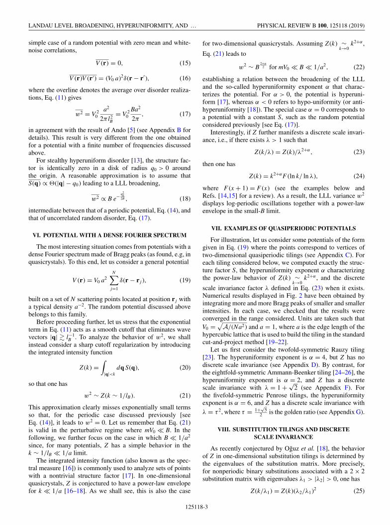
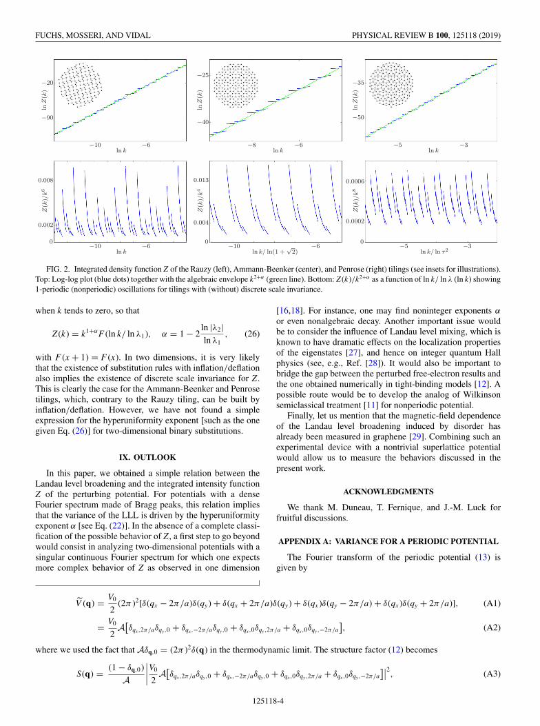
For illustration, let us consider some potentials of the formgiven in Eq. (19) where the points correspond to vertices oftwo-dimensional quasiperiodic tilings (see Appendix C). Foreach tiling considered below, we computed exactly the struc-ture factor S, the hyperuniformity exponent α characterizingthe power-law behavior of Z (k) ∼
k→0k2+α , and the discrete
scale invariance factor λ defined in Eq. (23) when it exists.Numerical results displayed in Fig. 2 have been obtained byintegrating more and more Bragg peaks of smaller and smallerintensities. In each case, we checked that the results wereconverged in the range considered. Units are taken such thatV0 =
√A/(Na2) and a = 1, where a is the edge length of the
hypercubic lattice that is used to build the tiling in the standardcut-and-project method [19–22].
Let us first consider the twofold-symmetric Rauzy tiling[23]. The hyperuniformity exponent is α = 4, but Z has nodiscrete scale invariance (see Appendix D). By contrast, forthe eightfold-symmetric Ammann-Beenker tiling [24–26], thehyperuniformity exponent is α = 2, and Z has a discretescale invariance with λ = 1 + √
2 (see Appendix F). Forthe fivefold-symmetric Penrose tilings, the hyperuniformityexponent is α = 6, and Z has a discrete scale invariance withλ = τ 2, where τ = 1+√
52 is the golden ratio (see Appendix G).
VIII. SUBSTITUTION TILINGS AND DISCRETESCALE INVARIANCE
As recently conjectured by Oguz et al. [18], the behaviorof Z in one-dimensional substitution tilings is determined bythe eigenvalues of the substitution matrix. More precisely,for nonperiodic binary substitutions associated with a 2 × 2substitution matrix with eigenvalues λ1 > |λ2| > 0, one has
Z (k/λ1) = Z (k)(λ2/λ1)2 (25)
125118-3
FUCHS, MOSSERI, AND VIDAL PHYSICAL REVIEW B 100, 125118 (2019)ln
Z(k
)
−20
−90
ln k−10 −6
Z(k
)/k6
0.008
0.002
0
ln k−10 −6
lnZ
(k)
−25
−40
ln k−8 −6
Z(k
)/k4
0.013
0.004
0
ln k/ ln(1 +√
2)−10 −6
lnZ
(k)
−35
−50
ln k−5 −3
Z(k
)/k8
0.0006
0.0002
0
ln k/ ln τ2−5 −3
FIG. 2. Integrated density function Z of the Rauzy (left), Ammann-Beenker (center), and Penrose (right) tilings (see insets for illustrations).Top: Log-log plot (blue dots) together with the algebraic envelope k2+α (green line). Bottom: Z (k)/k2+α as a function of ln k/ ln λ (ln k) showing1-periodic (nonperiodic) oscillations for tilings with (without) discrete scale invariance.
when k tends to zero, so that
Z (k) = k1+αF (ln k/ ln λ1), α = 1 − 2ln |λ2|ln λ1
, (26)
with F (x + 1) = F (x). In two dimensions, it is very likelythat the existence of substitution rules with inflation/deflationalso implies the existence of discrete scale invariance for Z .This is clearly the case for the Ammann-Beenker and Penrosetilings, which, contrary to the Rauzy tiling, can be built byinflation/deflation. However, we have not found a simpleexpression for the hyperuniformity exponent [such as the onegiven Eq. (26)] for two-dimensional binary substitutions.
IX. OUTLOOK
In this paper, we obtained a simple relation between theLandau level broadening and the integrated intensity functionZ of the perturbing potential. For potentials with a denseFourier spectrum made of Bragg peaks, this relation impliesthat the variance of the LLL is driven by the hyperuniformityexponent α [see Eq. (22)]. In the absence of a complete classi-fication of the possible behavior of Z , a first step to go beyondwould consist in analyzing two-dimensional potentials with asingular continuous Fourier spectrum for which one expectsmore complex behavior of Z as observed in one dimension
[16,18]. For instance, one may find noninteger exponents α
or even nonalgebraic decay. Another important issue wouldbe to consider the influence of Landau level mixing, which isknown to have dramatic effects on the localization propertiesof the eigenstates [27], and hence on integer quantum Hallphysics (see, e.g., Ref. [28]). It would also be important tobridge the gap between the perturbed free-electron results andthe one obtained numerically in tight-binding models [12]. Apossible route would be to develop the analog of Wilkinsonsemiclassical treatment [11] for nonperiodic potential.
Finally, let us mention that the magnetic-field dependenceof the Landau level broadening induced by disorder hasalready been measured in graphene [29]. Combining such anexperimental device with a nontrivial superlattice potentialwould allow us to measure the behaviors discussed in thepresent work.
ACKNOWLEDGMENTS
We thank M. Duneau, T. Fernique, and J.-M. Luck forfruitful discussions.
APPENDIX A: VARIANCE FOR A PERIODIC POTENTIAL
The Fourier transform of the periodic potential (13) isgiven by
V (q) = V0
2(2π )2[δ(qx − 2π/a)δ(qy) + δ(qx + 2π/a)δ(qy) + δ(qx )δ(qy − 2π/a) + δ(qx )δ(qy + 2π/a)], (A1)
= V0
2A
[δqx,2π/aδqy,0 + δqx,−2π/aδqy,0 + δqx,0δqy,2π/a + δqx,0δqy,−2π/a
], (A2)
where we used the fact that Aδq,0 = (2π )2δ(q) in the thermodynamic limit. The structure factor (12) becomes
S(q) = (1 − δq,0)
A
∣∣∣∣V0
2A
[δqx,2π/aδqy,0 + δqx,−2π/aδqy,0 + δqx,0δqy,2π/a + δqx,0δqy,−2π/a
]∣∣2, (A3)
125118-4
LANDAU LEVEL BROADENING, HYPERUNIFORMITY, AND … PHYSICAL REVIEW B 100, 125118 (2019)
= V 20
4A
[δqx,2π/aδqy,0 + δqx,−2π/aδqy,0 + δqx,0δqy,2π/a + δqx,0δqy,−2π/a
], (A4)
= V 20
4(2π )2[δ(qx − 2π/a)δ(qy) + δ(qx + 2π/a)δ(qy) + δ(qx )δ(qy − 2π/a) + δ(qx )δ(qy + 2π/a)], (A5)
where we used the Kronecker delta in order to computethe modulus square of the Fourier transform (otherwise, thesquare of a Dirac δ is ill-defined). Then Eq. (11) involves theintegral of Dirac δ functions, which straightforwardly leads toEq. (14).
APPENDIX B: VARIANCE FOR A RANDOM POTENTIAL
The Fourier transform of the uncorrelated random potentialdefined by Eqs. (15) and (16) is given by
V (q) =∫
dr e−ir·qV (r) = 0
and
|V (q)|2 =∫
dr e−ir·q∫
dr′eir′ ·qV (r)V (r′) = (V0a)2A.
The structure factor (12) becomes S(q) = (V0a)2(1 − δq,0).In Eq. (11), the Kronecker delta does not contribute, and theGaussian integral gives Eq. (17):
w2 = (V0a)2
(2π )2
∫dq e−|q|2l2
B/2 = (V0a)2
(2π )2
2π
l2B
.
APPENDIX C: FOURIER TRANSFORMOF A CUT-AND-PROJECT QUASICRYSTAL
The cut-and-project (CP) method [19–22] consists in se-lecting points of a D-dimensional periodic lattice if theirprojection onto the (D − d )-dimensional perpendicular spaceE⊥ belongs to a so-called acceptance window. The tiling isthen obtained by projecting these selected points onto thecomplementary d-dimensional parallel space E‖.
Any vector v in hyperspace can be decomposed uniquelyin terms of its projection onto parallel and perpendicularspaces as
v = v‖ + v⊥. (C1)
As explained in the early papers introducing the CP method[20–22], the Fourier transform of quasiperiodic tilings can becomputed from the higher-dimensional space from which itstems. The main idea is that since points of the tiling areselected from a periodic tiling via an acceptance window,computing the Fourier transform of the tiling essentiallyamounts to computing the Fourier transform of this accep-tance window.
For a tiling with N sites (vertices) at position R‖j and
obtained by the CP method, the microscopic density is
n(r‖) =N∑
j=1
δ(r‖ − R‖j ), (C2)
and its Fourier transform is
n(q‖) =N∑
j=1
e−i q‖·R‖j , (C3)
where the sum runs over all sites of the d-dimensional tilingconsidered. The convention that we use is that upper-caseletters (such as R‖
j ) refer to discrete points, and lower-caseletters (such as r‖) refer to a continuum of points.
Let R be a point of the D-dimensional hypercubic lattice,and let K be a vector of its reciprocal lattice such thatK · R = 2π × integer. These vectors can be decomposed ontothe parallel and perpendicular spaces such that their scalarproduct reads
K · R = K‖ · R‖ + K⊥ · R⊥ = 2π × integer. (C4)
Equation (C3) is nonzero iff q‖ = K‖, in which case it be-comes
n(K‖) =N∑
j=1
ei K⊥·R⊥j . (C5)
For a quasicrystal built along an irrational plane (parallelspace), the points in perpendicular space densely and uni-formly fill the acceptance window such that
n(K‖) = N∫A⊥
dr⊥A⊥
ei K⊥·r⊥ , (C6)
where the integral is over the acceptance window in perpen-dicular space, and A⊥ is its (D − d )-dimensional volume.
Now, for any vector q‖ in parallel space, the Fouriertransform of the density Eq. (C3) reads
n(q‖) =∑
K
δq‖,K‖N∫A⊥
dr⊥A⊥
ei K⊥·r⊥ , (C7)
where the sum is performed over all vectors K of the recip-rocal lattice of the hypercubic lattice. As we are consideringa quasicrystal, for any K‖ there is a unique K and thereforeK⊥ is well-defined. If {a∗
j ; j = 1, . . . , D} is a basis of vectorsin reciprocal space, then K = ∑
j n ja∗j , where n j are integers.
Its parallel and perpendicular components are also functionsof the same integers:
K = K‖(n1, . . . , nD) + K⊥(n1, . . . , nD). (C8)
Therefore, the sum over K in Eq. (C7) is actually a sumover D integers n1, . . . , nD, clearly showing that the Fouriertransform is a pure point of rank D > d .
Let us define the structure factor in the thermodynamiclimit as
S(q‖) = |n(q‖)|2N
(1 − δq‖,0). (C9)
For two-dimensional potentials (d = 2) of the form given byEq. (19), this definition differs from the one given in Eq. (12)
125118-5
FUCHS, MOSSERI, AND VIDAL PHYSICAL REVIEW B 100, 125118 (2019)
by a factor V 20 a4N/A, which disappears upon choosing units
such that V0 =√A/(Na2).
As explained in Ref. [17], for a spectrum made of a denseset of Bragg peaks (discontinuous S), the integrated intensityfunction
Z (k) =∫
|q‖|<kS(q‖) dq‖ (C10)
provides a reliable characterization of the point distribution.Here, the integral is performed over a disk of radius k. Thisfunction is also known as the spectral measure in Ref. [16].
For d-dimensional tilings built by the CP method, thisquantity can be recast in the following form:
Z (k) = (2π )d
A∑
|K‖|<k
S(K‖). (C11)
APPENDIX D: THE RAUZY TILING
1. Fourier transform
The two-dimensional (generalized) Rauzy tiling has beenintroduced in Ref. [23]. This is a codimension-1 tiling builtfrom the cubic lattice Z3 (edge length a = 1) with a one-dimensional perpendicular space oriented along the directione⊥ = (θ2, θ, 1), where θ is the real (Pisot-Vijayaraghavan)root of the cubic equation x3 = x2 + x + 1. Contrary to theAmmann-Beenker and the Penrose tilings discussed in thenext Appendixes, the Rauzy tiling cannot be built by substitu-tion rules.
For such a codimension-1 quasicrystal, the acceptancewindow is a segment of length A⊥ defined as the projectionof h = (1, 1, 1) onto the perpendicular space. This acceptancewindow also corresponds to the projection of the unit cubeonto the perpendicular space. In this case, Eq. (C6) gives
|n(K‖)| = N
∣∣∣∣sinc
(K⊥ · h⊥
2
)∣∣∣∣. (D1)
2. Structure factor
The structure factor is defined in Eq. (C9). Our goal is toanalyze the behavior of S(q‖) in the limit where |q‖| tendsto zero. By definition, one has S(0) = 0, but its behavior
for small |q‖| is nontrivial since S(q‖) �= 0 only when q‖coincides with the parallel component K‖ of a reciprocal-lattice vector K of the cubic lattice. Thus, we are interested incomputing the behavior of S when |K‖| goes to 0 for K‖ �= 0:
S(K‖) = N
∣∣∣∣∣ sin(K⊥·h⊥
2
)K⊥·h⊥
2
∣∣∣∣∣2
, (D2)
= N
∣∣∣∣∣ sin(K‖·h‖
2
)K⊥·h⊥
2
∣∣∣∣∣2
, (D3)
�|K‖|→0
N
∣∣∣∣ K‖ · h‖K⊥ · h⊥
∣∣∣∣2
, (D4)
where we used the fact that K is a reciprocal-lattice vector andh is a direct-lattice vector. The difficulty comes from the factthat, when |K‖| goes to 0, |K⊥| diverges. So, the goal is to findthe relation between these two components.
One way to investigate this issue is to follow the ap-proach proposed in Ref. [17] for the Fibonacci chain (seeAppendix E). In the Z3 canonical basis, any reciprocal-latticevector K has coordinates 2π (l, m, n), where l, m, and n areintegers. To analyze the behavior of K‖ · h‖ and K⊥ · h⊥, letus consider the matrix
M =⎛⎝1 1 1
1 0 00 1 0
⎞⎠, (D5)
which satisfies M3 = M2 + M + 1. The eigenvalues of M arethe Tribonacci constant θ � 1.8393 and two complex conju-gate eigenvalues e±iφ/
√θ with φ � 2.1762. The eigenvector
associated with θ corresponds to the perpendicular directione⊥. Since θ is a Pisot-Vijayaraghavan number, the action ofM p onto any vector v, such that v · e⊥ �= 0, drives this vectortoward the direction e⊥ in the large-p limit.
Hence, to analyze the behavior of S in the limit where K‖tends to zero [see Eq. (D5)], let us consider K(p) = M pK.More precisely, we are interested in computing K(p)
‖ · h‖and K(p)
⊥ · h⊥. Keeping in mind that h⊥ = P⊥(1, 1, 1) andh‖ = (1 − P⊥)(1, 1, 1) (where P⊥ is the projector onto theperpendicular space), one can easily compute these quantities.After some algebra, one gets
K(p)‖ · h‖ = (θ − 1)θ− p+1
2 {sin(pφ)[(1 + θ2)m − θ (l + n)] + √θ{(θm − l ) sin[(1 + p)φ] + (θn − m) sin[(1 − p)φ]}}
sin(φ)[(θ − 1)θ + 1],
(D6)
K(p)⊥ · h⊥ = 1
sin(φ)[(θ − 1)θ + 1][2θ3/2 cos(φ) − θ3 − 1]{−θ p(θ4 + θ2 + 1) sin(φ)(θ l − 2
√θm cos(φ) + n)
+ θ− p−12 [θ3/2 sin[(p + 1)φ][(θ − 1)l + θ2(n − m)] + (θ − 1)θ sin(pφ)[l − (θ + 1)m + θn]
+√
θ sin[(p − 1)φ][−l + m + (θ − 1)θn] + θ3(l − θm) sin[(p + 2)φ] + (m − θn) sin[(p − 2)φ]]}. (D7)
Thus, in the large-p limit, one finds that K(p)‖ · h‖ vanishes as θ−p/2, K(p)
⊥ · h⊥ diverges as θ p, and S(K(p)‖ ) behaves as θ−3p.
As a result, one finds that
S(K‖) ∼|K‖|→0
|K‖|6 (D8)
125118-6
LANDAU LEVEL BROADENING, HYPERUNIFORMITY, AND … PHYSICAL REVIEW B 100, 125118 (2019)
for all (l, m, n). However, we emphasize that, contrary tothe Fibonacci chain Ref. [17] (see also Appendix E), thispower-law behavior is modulated by a bounded oscillatingnonperiodic function, as can be seen in Eqs. (D6) and (D7).
3. Integrated intensity function
The integrated intensity function is defined in Eq. (C11).The sum over all vector K‖ with a norm smaller than k canbe decomposed into a sum over all triplets (l, m, n) and theiriterated under M p. As a result, one has
Z (k) = 4π2
A∑
(l,m,n)
∞∑p=p(l,m,n)
S(K(p)‖ ), (D9)
where p(l,m,n) is the smallest integer fulfilling the constraint|K(p)
‖ | < k. As already discussed in the previous section, inthe large-p limit,
S(K(p)‖ ) � |K(p)
‖ |6 f (l, m, n, p), (D10)
|K(p)‖ | � θ−p/2g(l, m, n, p), (D11)
where, for a given triplet (l, m, n), f and g are boundedoscillating functions of p [see Eqs. (D6) and (D7)]). Thus, Sis bounded both above and below,
Z−(k) � Z (k) � Z+(k), (D12)
where
Z±(k) = 4π2
A∑
(l,m,n)
c±(l, m, n)∞∑
p=p(l,m,n)
θ−3p, (D13)
c+(l, m, n) = maxp
f (l, m, n, p)6g(l, m, n, p), (D14)
c−(l, m, n) = minp
f (l, m, n, p)6g(l, m, n, p). (D15)
Interestingly, Z±(k/√
θ ) = Z±(k)/θ3, as can be seen fromEqs. (D10) and (D11), since dividing k by
√θ simply amounts
to changing p(l,m,n) into p(l,m,n) + 1 in Eq. (D13). Such arelation reflects a discrete scale invariance [14] (see also thenext Appendix) for Z± and implies a power-law envelope
Z (k) ∼k→0
k6. (D16)
Note that, despite the fact that Z is defined as an integralof S, they are both characterized by a power law with thesame exponent. This is a consequence of the fact that S isdiscontinuous (discrete) and dense.
APPENDIX E: INTEGRATED INTENSITY FUNCTIONOF THE FIBONACCI CHAIN
The Fibonacci chain is a one-dimensional tiling built fromthe square lattice Z2 (edge length a = 1). The integratedintensity function Z of the Fibonacci chain has been widelydiscussed in Ref. [17]. However, one important property hasbeen missed. As a codimension-1 system, the Fourier trans-form of the Fibonacci chain can be easily computed. The
structure factor is
S(K‖) = N
∣∣∣∣∣ sin(K‖.h‖
2
)K⊥.h⊥
2
∣∣∣∣∣2
, (E1)
where h‖ and h⊥ are the projections of the vectorh = (1, 1) onto e‖ = 1√
1+τ 2 (−1, τ ) and e⊥ = 1√1+τ 2 (τ, 1),
where τ = 1+√5
2 is the golden ratio. The integrated intensityfunction is then
Z (k) = 2π
A∑
|K‖|<k
S(K‖), (E2)
where A is the total length of the chain. As for the Rauzytiling, let us consider the matrix
M =(
1 11 0
), (E3)
which satisfies M2 = M + 1. Eigenspaces of M correspond tothe perpendicular and parallel directions with eigenvalues τ
and −1/τ , respectively. The small-k behavior of Z is obtainedby analyzing sequences K(p) = M pK (see Ref. [17]). Onethen gets, in the large-p limit,
S(K(p)‖ ) � |K(p)
‖ |4 f (l, m), (E4)
|K(p)‖ | � τ−pg(l, m). (E5)
However, contrary to the Rauzy tiling, f and g do not dependon p. Thus, following the same line of reasoning as above, onestraightforwardly gets the discrete scaling relation
Z (k/τ ) = Z (k)/τ 4. (E6)
The solution of this equation can be written as
Z (k) = k4F (ln k/ ln τ ), (E7)
where F (x + 1) = F (x) (for a review on discrete scale in-variance, see Ref. [14]). As a result, Z has a power-lawenvelope together with log-periodic oscillations (see Fig. 3for illustration). This is in stark contrast with the Rauzy tilingwhere only Z+ and Z− obey such a discrete scale invariancebut not Z itself. Practically, to compute Z , we first selecta set of K points in the reciprocal lattice of Z2 inside agiven ball of radius Kmax around the origin. For each ofthese points, we consider the sequence of points K(p) withp = 0, . . . , pmax, and we compute S for each correspondingK(p)
‖ (avoiding possible redundancy). Z is then obtained bysumming over these Bragg peaks according to Eq. (E2). Wecheck the convergence of the results displayed in Fig. 3 byincreasing Kmax and pmax.
APPENDIX F: THE OCTAGONAL TILING
1. Fourier transform
The octagonal (Ammann-Beenker) tiling [24–26] is acodimension-2 tiling built from the four-dimensional hypercu-bic lattice Z4 (edge length a = 1). Perpendicular and parallel
125118-7
FUCHS, MOSSERI, AND VIDAL PHYSICAL REVIEW B 100, 125118 (2019)ln
Z(k
)
−12
−24
ln k
−4 −2
Z(k
)/k4
0.001
0.0035
ln k/ ln τ
−9 −6 −3
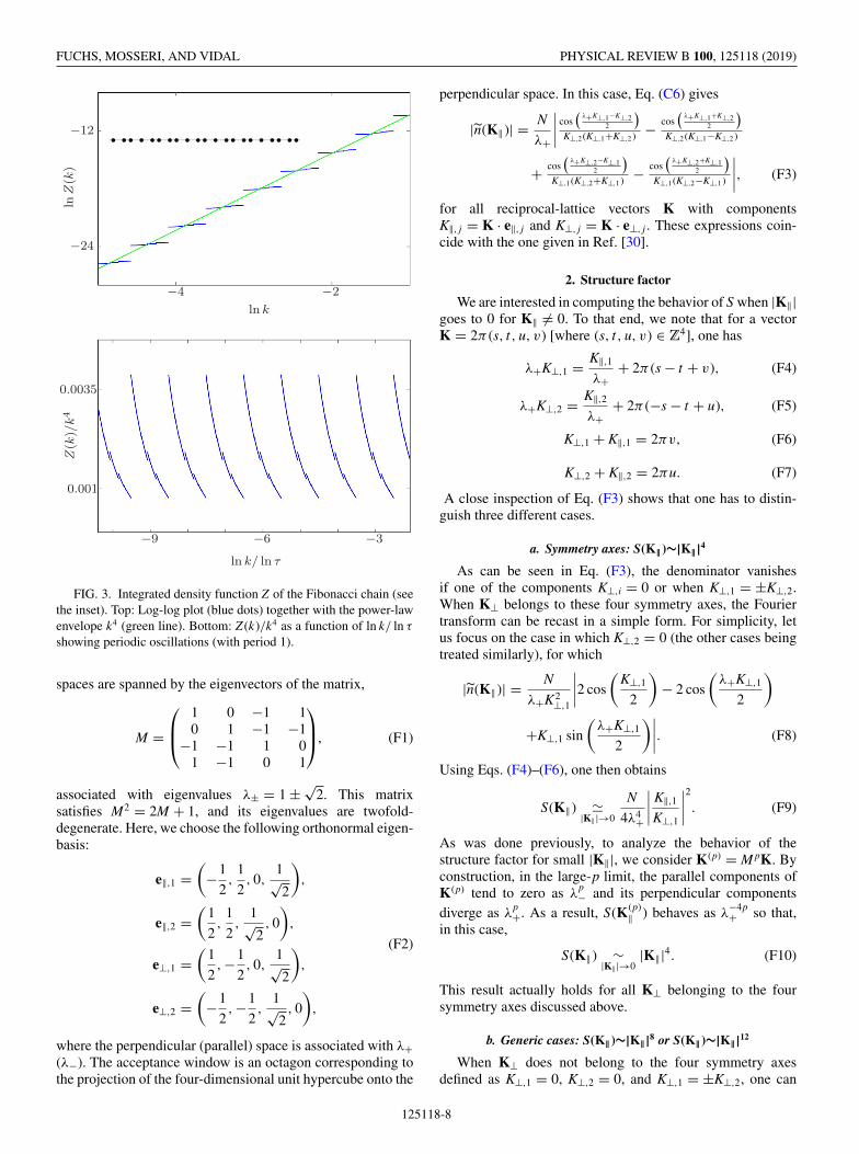
FIG. 3. Integrated density function Z of the Fibonacci chain (seethe inset). Top: Log-log plot (blue dots) together with the power-lawenvelope k4 (green line). Bottom: Z (k)/k4 as a function of ln k/ ln τ
showing periodic oscillations (with period 1).
spaces are spanned by the eigenvectors of the matrix,
M =
⎛⎜⎝
1 0 −1 10 1 −1 −1
−1 −1 1 01 −1 0 1
⎞⎟⎠, (F1)
associated with eigenvalues λ± = 1 ± √2. This matrix
satisfies M2 = 2M + 1, and its eigenvalues are twofold-degenerate. Here, we choose the following orthonormal eigen-basis:
e‖,1 =(
−1
2,
1
2, 0,
1√2
),
e‖,2 =(
1
2,
1
2,
1√2, 0
),
(F2)
e⊥,1 =(
1
2,−1
2, 0,
1√2
),
e⊥,2 =(
−1
2,−1
2,
1√2, 0
),
where the perpendicular (parallel) space is associated with λ+(λ−). The acceptance window is an octagon corresponding tothe projection of the four-dimensional unit hypercube onto the
perpendicular space. In this case, Eq. (C6) gives
|n(K‖)| = N
λ+
∣∣∣∣ cos(
λ+K⊥,1−K⊥,22
)K⊥,2(K⊥,1+K⊥,2 ) − cos
(λ+K⊥,1+K⊥,2
2
)K⊥,2(K⊥,1−K⊥,2 )
+ cos(
λ+K⊥,2−K⊥,12
)K⊥,1(K⊥,2+K⊥,1 ) − cos
(λ+K⊥,2+K⊥,1
2
)K⊥,1(K⊥,2−K⊥,1 )
∣∣∣∣, (F3)
for all reciprocal-lattice vectors K with componentsK‖, j = K · e‖, j and K⊥, j = K · e⊥, j . These expressions coin-cide with the one given in Ref. [30].
2. Structure factor
We are interested in computing the behavior of S when |K‖|goes to 0 for K‖ �= 0. To that end, we note that for a vectorK = 2π (s, t, u, v) [where (s, t, u, v) ∈ Z4], one has
λ+K⊥,1 = K‖,1λ+
+ 2π (s − t + v), (F4)
λ+K⊥,2 = K‖,2λ+
+ 2π (−s − t + u), (F5)
K⊥,1 + K‖,1 = 2πv, (F6)
K⊥,2 + K‖,2 = 2πu. (F7)
A close inspection of Eq. (F3) shows that one has to distin-guish three different cases.
a. Symmetry axes: S(K‖)∼|K‖|4
As can be seen in Eq. (F3), the denominator vanishesif one of the components K⊥,i = 0 or when K⊥,1 = ±K⊥,2.When K⊥ belongs to these four symmetry axes, the Fouriertransform can be recast in a simple form. For simplicity, letus focus on the case in which K⊥,2 = 0 (the other cases beingtreated similarly), for which
|n(K‖)| = N
λ+K2⊥,1
∣∣∣∣2 cos
(K⊥,1
2
)− 2 cos
(λ+K⊥,1
2
)
+K⊥,1 sin
(λ+K⊥,1
2
)∣∣∣∣. (F8)
Using Eqs. (F4)–(F6), one then obtains
S(K‖) �|K‖|→0
N
4λ4+
∣∣∣∣ K‖,1K⊥,1
∣∣∣∣2
. (F9)
As was done previously, to analyze the behavior of thestructure factor for small |K‖|, we consider K(p) = M pK. Byconstruction, in the large-p limit, the parallel components ofK(p) tend to zero as λ
p− and its perpendicular components
diverge as λp+. As a result, S(K(p)
‖ ) behaves as λ−4p+ so that,
in this case,
S(K‖) ∼|K‖|→0
|K‖|4. (F10)
This result actually holds for all K⊥ belonging to the foursymmetry axes discussed above.
b. Generic cases: S(K‖)∼|K‖|8 or S(K‖)∼|K‖|12
When K⊥ does not belong to the four symmetry axesdefined as K⊥,1 = 0, K⊥,2 = 0, and K⊥,1 = ±K⊥,2, one can
125118-8
LANDAU LEVEL BROADENING, HYPERUNIFORMITY, AND … PHYSICAL REVIEW B 100, 125118 (2019)
again use Eqs. (F4)–(F7) to express the structure factor as
S(K‖)
�|K‖|→0
N
4λ4+
∣∣∣∣ (K‖,1K⊥,2+K‖,2K⊥,1)(K‖,1K⊥,1−K‖,2K⊥,2)
K⊥,1K⊥,2(K⊥,1+K⊥,2)(K⊥,1−K⊥,2)
∣∣∣∣2
,
(F11)
which leads to
S(K‖) ∼|K‖|→0
|K‖|8. (F12)
However, as can be seen in Eq. (F11), this leading contributionmay vanish for some special K. In this case, S is given by thesubleading contribution, which gives
S(K‖) ∼|K‖|→0
|K‖|12. (F13)
3. Integrated intensity function
To compute the integrated intensity function defined inEq. (C11), we decompose the sum over all vector K‖ witha norm smaller than k as a sum over all quadruplets (s, t, u, v)and their iterated vectors K(p)
‖ = M pK‖. One can then write
Z (k) = 4π2
A∑
(s,t,u,v)
∞∑p=p(s,t,u,v)
S(K(p)‖ ), (F14)
where p(s,t,u,v) is the smallest integer fulfilling the constraint|K(p)
‖ | < k. As discussed above, the behavior of S in the large-p (small-|K‖|) limit strongly depends on K‖ [see Eqs. (F10)–(F13)]. This is in stark contrast with the Rauzy tiling and theFibonacci chain, where there is the same power-law scalingfor all K‖ [see Eqs. (D10)–(E4)].
However, since we are interested in the small-k (large-p)limit, one only keeps the dominant terms in Eq. (F14) thatcome from the symmetry axes and gives
S(K(p)‖ ) � |K(p)
‖ |4 f (s, t, u, v), (F15)
|K(p)‖ | � λ
−p+ g(s, t, u, v). (F16)
We emphasize that, as for the Fibonacci chain, f and g arefunctions that do not depend on p, so that one straightfor-wardly gets the following discrete scaling relation:
Z (k/λ+) = Z (k)/λ4+. (F17)
The solution of this equation can be written as
Z (k) = k4F (ln k/ ln λ+), (F18)
where F (x + 1) = F (x). As a result, Z has a power-lawenvelope together with log-periodic oscillations.
APPENDIX G: THE PENROSE TILING
The Penrose rhombus tiling [19,31] can be built by CPfrom the five-dimensional hypercubic lattice Z5 (edge lengtha = 1) along a well-known procedure (see, e.g., Ref. [32]for details). For our purpose, let us consider the followingorthogonal (non-normalized) basis:
e‖,1 = 25 (1, c2, c4, c4, c2),
e‖,2 = 25 (0, s2, s4,−s4,−s2),
e⊥,1 = 25 (1, c4, c2, c2, c4),
e⊥,2 = 25 (0, s4,−s2, s2,−s4),
e = 110 (1, 1, 1, 1, 1), (G1)
which defines the three subspaces E‖, E⊥, and . Here, we in-troduced the notation cn = cos(2πn/5) and sn = sin(2πn/5).A point in Z5 is selected whenever it projects onto the perpen-dicular space E⊥ + inside a three-dimensional acceptancewindow which is the projection of the five-dimensional unithypercube onto this subspace. Remarkably, selected pointsonly fill five planes perpendicular to . Thus, the selectionstep only amounts to considering discrete sections of theacceptance window. Among all possible choices, the fivefold-symmetric canonical Penrose tilings (known as star and sun[25]) considered here correspond to the following sections:One point that is the symmetry center of the tiling, tworegular pentagons of side 2
√2/5 cos(3π/10), and two regular
pentagons of side 2 τ√
2/5 cos(3π/10), where τ = 1+√5
2 isthe golden ratio.
1. Fourier transform
The Fourier transform of the tiling’s vertices is obtained asa weighted sum of the Fourier transform of the four regularpentagons. For any vector R of the five-dimensional hyper-cubic lattice, the five-dimensional reciprocal lattice vectors Ksatisfy
K · R = K‖ · R‖ + K⊥ · R⊥ + K · R = 2π × integer.
(G2)
Then, after some algebra, Eq. (C6) leads to
|n(K‖ )| = N
∣∣∣∣ 8(s2 − s4)
5K⊥,2
{cos(c2K⊥,1 + s2K⊥,2 − 3K ) + cos[K⊥,1/2 + (s4 + s2)K⊥,2 + K ] − cos(K⊥,1 − 3K ) − cos(2c4K⊥,1 − K )
5K⊥,1 − (6s2 + 2s4)K⊥,2
− cos(c2K⊥,1 − s2K⊥,2 − 3K ) + cos[K⊥,1/2 − (s4 + s2)K⊥,2 + K ] − cos(K⊥,1 − 3K ) − cos(2c4K⊥,1 − K )
5K⊥,1 + (6s2 + 2s4)K⊥,2
+ cos(c2K⊥,1 − s2K⊥,2 − 3K ) + cos[K⊥,1/2 − (s4 + s2)K⊥,2 + K ] − cos(c4K⊥,1 − s4K⊥,2 − 3K ) − cos[(1 + c2)K⊥,1 + s2K⊥,2 − K ]
5K⊥,1 − (6s4 − 2s2)K⊥,2
− cos(c2K⊥,1 + s2K⊥,2 − 3K ) + cos[K⊥,1/2 + (s4 + s2)K⊥,2 + K ] − cos(c4K⊥,1 + s4K⊥,2 − 3K ) − cos[(1 + c2)K⊥,1 − s2K⊥,2 − K ]
5K⊥,1 + (6s4 − 2s2)K⊥,2
}∣∣∣∣(G3)
for all reciprocal-lattice vectors K with components K‖, j = K · e‖, j , K⊥, j = K · e⊥, j , and K = K · e .
125118-9
FUCHS, MOSSERI, AND VIDAL PHYSICAL REVIEW B 100, 125118 (2019)
2. Structure factor
We are interested in computing the behavior of S when |K‖| goes to 0 for K‖ �= 0. To that end, we note that for a vectorK = 2π (s, t, u, v,w) [where (s, t, u, v,w) ∈ Z5], one has
c2K⊥,1 + s2K⊥,2 − 3K = −c4K‖,1 + s4K‖,2 − 5K + 2πv, (G4)
c2K⊥,1 − s2K⊥,2 − 3K = −c4K‖,1 − s4K‖,2 − 5K + 2πu, (G5)
K⊥,1/2 + (s4 + s2)K⊥,2 + K = −K‖,1/2 + (s4 − s2)K‖,2 + 5K − 2π (u + w), (G6)
K⊥,1/2 − (s4 + s2)K⊥,2 + K = −K‖,1/2 − (s4 − s2)K‖,2 + 5K − 2π (v + t ), (G7)
K⊥,1 − 3K = −K‖,1 − 5K + 2πs, (G8)
2c4K⊥,1 − K = −2c2K‖,1 − 5K + 2π (t + w), (G9)
c4K⊥,1 + s4K⊥,2 − 3K = −c2K‖,1 − s2K‖,2 − 5K + 2πt, (G10)
c4K⊥,1 − s4K⊥,2 − 3K = −c2K‖,1 + s2K‖,2 − 5K + 2πw, (G11)
(1 + c2)K⊥,1 + s2K⊥,2 − K = −(1 + c4)K‖,1 + s4K⊥,2 − 5K + 2π (s + v), (G12)
(1 + c2)K⊥,1 − s2K⊥,2 − K = −(1 + c4)K‖,1 − s4K⊥,2 − 5K + 2π (s + u). (G13)
Keeping in mind that 5K = π (s + t + u + v + w), one can finally rewrite Eq. (G3) as a function of K‖, j and K⊥, j only. Inthe limit where |K‖| → 0, one then gets generically
S(K‖) �|K‖|→0
N (√
5 − 2)2
∣∣∣∣(K2
⊥,1 + K2⊥,2
)[(K2
‖,1 − K2‖,2)K⊥,2 − 2K‖,1K‖,2K⊥,1
]K⊥,2
(5K4
⊥,1 − 10K2⊥,1K2
⊥,2 + K4⊥,2
) ∣∣∣∣2
. (G14)
However, when one of the denominators in Eq. (G3) van-ishes, one gets different expressions that are easily obtainedalong the same lines.
To analyze the behavior of the structure factor for small|K‖|, we consider the matrix
M =
⎛⎜⎜⎜⎝
0 1 0 0 11 0 1 0 00 1 0 1 00 0 1 0 11 0 0 1 0
⎞⎟⎟⎟⎠, (G15)
whose eigenspaces are E‖, E⊥, and E with eigenvaluesλ‖ = 1/τ , λ⊥ = −τ , and λ = 2, respectively. By con-struction, in the large-p limit, the parallel components ofK(p) = M pK vanish as λ
p‖ , whereas its perpendicular compo-
nents diverge as λp⊥. As a result, in the large-p limit, S(K(p)
‖ )
behaves as λ8p‖ so that
S(K‖) ∼|K‖|→0
|K‖|8. (G16)
3. Integrated intensity function
As for the octagonal tiling, we decompose the sum overK‖ in the integrated intensity function defined in Eq. (C11)as a sum over all quintuplets (s, t, u, v,w) and their iteration
under K(p)‖ = M pK‖. One can then write
Z (k) = 4π2
A∑
(s,t,u,v,w)
∞∑p=p(s,t,u,v,w)
S(K(p)‖ ), (G17)
where p(s,t,u,v,w) is the smallest integer fulfilling the constraint|K(p)
‖ | < k. In the small-k (large-p) limit, one can check that
S(K(p)‖ ) � |K(p)
‖ |8 f (s, t, u, v,w) (G18)
for any quintuplet (s, t, u, v,w) ∈ Z5. However, contrary tothe octagonal tiling, the scaling of K(p)
‖ with p depends onthe quintuplet. For quintuplets that do not annihilate thedenominator in Eq. (G3), one gets
|K(p)‖ | � τ−pg(s, t, u, v,w), (G19)
or, in other words, |K(p)‖ /K(p+1)
‖ | = τ . Importantly, when oneof the denominators in Eq. (G3) vanishes, one gets a weakerrelation since one only has |K(p)
‖ /K(p+2)‖ | = τ 2. As a direct
consequence, one gets the following discrete scaling relation:
Z (k/τ 2) = Z (k)/τ 16. (G20)
The solution of this equation can be written as
Z (k) = k8F (ln k/ ln τ 2), (G21)
where F (x + 1) = F (x). As a result, Z has a power-lawenvelope together with log-periodic oscillations.
125118-10
LANDAU LEVEL BROADENING, HYPERUNIFORMITY, AND … PHYSICAL REVIEW B 100, 125118 (2019)
[1] K. v. Klitzing, G. Dorda, and M. Pepper, New Method forHigh-Accuracy Determination of the Fine-Structure ConstantBased on Quantized Hall Resistance, Phys. Rev. Lett. 45, 494(1980).
[2] K. v. Klitzing, The quantized Hall effect, Rev. Mod. Phys. 58,519 (1986).
[3] T. Ando and Y. Uemura, Theory of quantum transport in atwo-dimensional electron system under magnetic fields. I. Char-acteristics of level broadening and transport under strong fields,J. Phys. Soc. Jpn. 36, 959 (1974).
[4] T. Ando, Theory of quantum transport in a two-dimensionalelectron system under magnetic fields. II. Single-site approxi-mation under strong fields, J. Phys. Soc. Jpn. 36, 1521 (1974).
[5] T. Ando, Theory of quantum transport in a two-dimensionalelectron system under magnetic fields. III. Many-site approx-imation, J. Phys. Soc. Jpn. 37, 622 (1974).
[6] B. Huckestein, Scaling theory of the integer quantum Halleffect, Rev. Mod. Phys. 67, 357 (1995).
[7] A. Rauh, Degeneracy of landau levels in crystals, Phys. StatusSolidi B 65, K131 (1974).
[8] A. Rauh, On the broadening of landau levels in crystals, Phys.Status Solidi B 69, K9 (1975).
[9] D. R. Hofstadter, Energy levels and wave functions of Blochelectrons in rational and irrational magnetic fields, Phys. Rev. B14, 2239 (1976).
[10] F. H. Claro and G. H. Wannier, Magnetic subband structure ofelectrons in hexagonal lattices, Phys. Rev. B 19, 6068 (1979).
[11] M. Wilkinson, Critical properties of electron eigenstates inincommensurate systems, Proc. R. Soc. London A 391, 305(1984).
[12] J. N. Fuchs, R. Mosseri, and J. Vidal, Landau levels in qua-sicrystals, Phys. Rev. B 98, 165427 (2018).
[13] S. Torquato, Hyperuniform states of matter, Phys. Rep. 745, 1(2018).
[14] D. Sornette, Discrete-scale invariance and complex dimensions,Phys. Rep. 297, 239 (1998).
[15] E. Akkermans, Statistical mechanics and quantum fields onfractals, Contemp. Math. 601, 1 (2013).
[16] J. M. Luck, Cantor spectra and scaling of gap widths in deter-ministic aperiodic systems, Phys. Rev. B 39, 5834 (1989).
[17] E. C. Oguz, J. E. S. Socolar, P. J. Steinhardt, and S. Torquato,Hyperuniformity of quasicrystals, Phys. Rev. B 95, 054119(2017).
[18] E. C. Oguz, J. E. S. Socolar, P. J. Steinhardt, and S. Torquato,Hyperuniformity and anti-hyperuniformity in one-dimensionalsubstitution tilings, Acta Crystallogr. A 75, 3 (2019).
[19] N. de Bruijn, Algebraic theory of Penrose’s non-periodic tilingsof the plane. I, Indag. Math. Proc. Ser. A 84, 39 (1981).
[20] M. Duneau and A. Katz, Quasiperiodic Patterns, Phys. Rev.Lett. 54, 2688 (1985).
[21] P. A. Kalugin, A. Yu. Kitaev, and L. S. Levitov, Al0.86Mn0.14:A six-dimensional crystal, Pis’ma Zh. Eksp. Teor. Fiz. 41, 119(1985) [JETP Lett. 41, 145 (1985)].
[22] V. Elser, Indexing problems in quasicrystal diffraction, Phys.Rev. B 32, 4892 (1985).
[23] J. Vidal and R. Mosseri, Generalized quasiperiodic Rauzytilings, J. Phys. A 34, 3927 (2001).
[24] F. P. M. Beenker, Algebraic theory of non periodic tilings of theplane by two simple building blocks: A square and a rhombus,TH Report 82-WSK-04 (Technische Hogeschool, Eindhoven,1982).
[25] B. Grünbaum and G. C. Shephard, Tilings and Patterns (W. H.Freeman and Company, New York, 1987).
[26] M. Duneau, R. Mosseri, and C. Oguey, Approximants ofquasiperiodic structures generated by the inflation mapping,J. Phys. A 22, 4549 (1989).
[27] F. D. M. Haldane and K.Yang, Landau Level Mixing andLevitation of Extended States in Two Dimensions, Phys. Rev.Lett. 78, 298 (1997).
[28] S. Kivelson, D.-H. Lee, and S.-C. Zhang, Global phase diagramin the quantum Hall effect, Phys. Rev. B 46, 2223 (1992).
[29] M. Orlita, C. Faugeras, P. Plochocka, P. Neugebauer, G.Martinez, D. K. Maude, A.-L. Barra, M. Sprinkle, C. Berger,W. A. de Heer, and M. Potemski, Approaching the Dirac Pointin High-Mobility Multilayer Epitaxial Graphene, Phys. Rev.Lett. 101, 267601 (2008).
[30] T. Janssen, G. Chapuis, and M. De Boissieu, Aperiodic Crystals(Oxford University Press, Oxford, 2007). Note that our choiceof eigenbasis is different (e⊥,2 → −e⊥,2) and a sign mistake hasto be corrected in the third term of S2 (cf. p. 140 in the firstedition).
[31] R. Penrose, Pentaplexity: A class of non-periodic tilings of theplane, Math. Intell. 2, 32 (1979).
[32] M. Duneau and M. Audier, in Lectures on Quasicrystals, editedby F. Hippert and D. Gratias (Les Editions de Physique, LesUlis, 1994), p. 283.
125118-11