Embed Size (px)
Citation preview
1556-6013 (c) 2018 IEEE. Personal use is permitted, but republication/redistribution requires IEEE permission. See http://www.ieee.org/publications_standards/publications/rights/index.html for more information.
This article has been accepted for publication in a future issue of this journal, but has not been fully edited. Content may change prior to final publication. Citation information: DOI 10.1109/TIFS.2019.2895963, IEEETransactions on Information Forensics and Security
Large-Scale Empirical Study of Important FeaturesIndicative of Discovered Vulnerabilities to Assess
Application SecurityMengyuan Zhang, Xavier de Carné de Carnavalet, Lingyu Wang, Member, IEEE, Ahmed Ragab
Abstract—Existing research on vulnerability discovery modelsshows that the existence of vulnerabilities inside an applicationmay be linked to certain features, e.g., size or complexity, ofthat application. However, the applicability of such features todemonstrate the relative security between two applications isnot well studied, which may depend on multiple factors in acomplex way. In this paper, we perform the first large-scaleempirical study of the correlation between various features ofapplications and the abundance of vulnerabilities. Unlike existingwork, which typically focuses on one particular applicationresulting in limited successes, we focus on the more realisticissue of assessing the relative security level among differentapplications. To the best of our knowledge, this is the mostcomprehensive study of 780 real world applications involving6,498 vulnerabilities. We apply seven feature selection methods tonine feature subsets selected among 34 collected features, whichare then fed into six types of machine learning models, producing523 estimations. The predictive power of important featuresis evaluated using four different performance measures. Ourstudy reflects that the complexity of applications is not the onlyfactor in vulnerability discovery, and that human related factorscontribute to explaining the number of discovered vulnerabilitiesin an application.
Index Terms—Software Vulnerability Analysis, VulnerabilityDiscovery Model, Software Security, Machine Learning
I. INTRODUCTION
EXISTING research on vulnerability discovery models(VDMs) shows that vulnerabilities in an application may
be linked to certain features, e.g., size or complexity, of thatapplication (a more detailed review of related work will begiven in Section VI). Those findings lead to an interestingquestion, i.e., can we predict the existence of vulnerabilitiesin an application based on its features? However, as shown inmost existing works on VDMs, including those that focus onpredicting vulnerable components inside one application [1],[2], [3], [4], [5], [6] and those that aim to establish mathemat-ical models based on the historical vulnerability data of oneapplication [7], [8], the correlation between vulnerabilities andthe features of an application is usually not straightforward
M. Zhang, X. de Carné de Carnavalet, and L. Wang are withthe Concordia Institute for Information Systems Engineering (CI-ISE), Concordia University, H3G 1M8, Montreal, QC, Canada. E-mail:{mengy_zh,x_decarn,wang}@ciise.concordia.ca.
A. Ragab with the Mathematics and Industrial Engineering Department,École Polytechnique de Montréal, C.P. 6079, Succ. Centre-Ville, H3C 3A7,Montreal, QC, Canada, and the Department of Industrial Electronics andControl Engineering, Faculty of Electronic Engineering, Menoufia University,Menouf, 32952, Egypt. E-mail: [email protected].
The list of extracted features for the 780 GitHub repositories is availableupon request to the first author.
or reliable enough for such a prediction. For instance, thenumber of vulnerabilities in an application may not only beproportional to its size or complexity (as our study will show,no single feature is likely to have such prediction power). Inother words, the existence of vulnerabilities in one particularapplication may depend on multiple factors in a complex way,which is still largely unknown.
In this paper, unlike existing works that typically focus onfunction/file/component level and construct models from oneor a few applications, we focus on the more realistic issueof predicting the relative likelihood of vulnerabilities amonga large number of applications. To this end, we perform,to the best of our knowledge, the first large-scale empiricalstudy using machine learning techniques on the correlationbetween the abundance of vulnerabilities in an applicationand a rich collection of features. More specifically, our maincontributions are as follows. To the best of our knowledge, thisis the most comprehensive study to date involving 780 real-world software applications and 6,498 vulnerabilities. We ap-ply seven feature selection methods on a rich collection of ninesubsets of features that are then fed into six learning models.The predictive power has been evaluated using four differentperformance metrics including a correlation coefficient.
A. OverviewAn overview of our study is given below, and is illustrated
in Fig. 1.• First, we obtain a large-scale dataset of open-source appli-
cations from GitHub, each of which involves at least onevulnerability listed in NVD [9]. In Section II, we addressvarious challenges in the data collection, e.g., automati-cally identifying GitHub repositories, obtaining the accuratenumber of vulnerabilities and automating the labeling ofrepositories and mapping to products.
• Second, 34 features in total are extracted from the soft-ware applications. They fall into five different categories:popularity metrics, developer metrics, software propertymetrics, software metrics, and security metrics. To the bestof our knowledge, this is the first effort to combine diversefeatures at the software level. Besides the commonly usedfeatures on code complexity and developer activity [10], weintroduce popularity metrics to reflect the potential interestfrom attackers, software property metrics to indicate variousintrinsic properties of the software, and security metrics toillustrate the potential attack surface of the applications.This is detailed in Section II-E.
1556-6013 (c) 2018 IEEE. Personal use is permitted, but republication/redistribution requires IEEE permission. See http://www.ieee.org/publications_standards/publications/rights/index.html for more information.
This article has been accepted for publication in a future issue of this journal, but has not been fully edited. Content may change prior to final publication. Citation information: DOI 10.1109/TIFS.2019.2895963, IEEETransactions on Information Forensics and Security
Fig. 1: An overview of the study
• Third, to reduce errors during the prediction process dueto correlated or noisy features, we apply various featureselection and projection methods to extract nine subsets,including the original set of 34 features for reference and itsprojection using Principal Component Analysis (PCA) [11].
• Fourth, we study three research questions, as detailed inSection I-B, related to the predictive power based onthe aforementioned features, using both statistical analysisand learning-based models. In our study, we apply twostatistical analysis methods, namely, Pearson correlationand Kolmogorov-Smirnov test, to evaluate the discrimina-tive power of features. Nine feature subsets (seven fromfeature selection results, one with the original set and oneextracted from the PCA) are fed into six learning modelsto predict the number of vulnerabilities in the software. Weprovide detailed descriptions of the study and analysis ofthe prediction results in Section IV.
• Finally, we leverage t-SNE [12] to visualize our multi-dimensional dataset into two dimensions and observe sep-arable clusters for applications in Section IV-C. We inves-tigate the criteria behind this segregation and find that thesize of the projects plays an important role in groupingapplications. One of such groups is populated only by verylow numbers of CVEs.
B. Research Questions and Our Main Findings
A common belief is that the complexity of an application isthe main cause of vulnerabilities [3]. However, the reality ismore complex since many other factors may come into play.For example, in our GitHub dataset, the project opencms-core,1
780,638 lines of code, which has a lower complexity than theproject SiberianCMS,2 1,863,840 lines of code, actually turnsout to have a higher number of vulnerabilities. Upon closerexamination, we find that the project opencms-core was firstreleased 2,331 days ago and project SiberianCMS was onlyreleased 601 days ago. The latter project contains a lowernumber of vulnerabilities, likely due to having a smaller timewindow for attackers to exploit. In this case, the complexityis clearly not the only determining feature. Similarly, we findthrough other examples that any type of features, e.g., the
1https://github.com/alkacon/opencms-core2https://github.com/Xtraball/SiberianCMS
age (the days counted from the release time until now) or thepopularity (the number of stars, watches, and forks), alone isnot likely to yield reliable prediction power. Therefore, we setup three research questions and summarize our main findingsas follows. We use #CVEs to represent the number of CVEsin the following sections.
• R1: Is there just one feature that is significantly correlatedwith the number of vulnerabilities in different applications?Our Finding: In the literature, a correlation coefficient ofless than 0.3 corresponds to a weak correlation, 0.3–0.5 toa medium correlation, and greater than 0.5 means a strongcorrelation [3]. If we follow the same interpretation, onlytwo features fall into medium correlation; the number ofcommits from our developer metrics and the application’sage. The rest of the features are only weakly correlated to#CVEs. In the later discriminative test, all the features arerejected in the K-S test with a small p-value.The conclusion we draw from this research question is thatinstead of complexity, human factors share higher correla-tion with #CVEs. Indeed, the number of commits (fromour developer metrics) and the application’s age (fromsoftware property metrics, although it also indicates theattack windows for an application) share medium positivecorrelation with #CVEs. However, even highly correlatedfeatures follow a different distribution than that of #CVEs.
• R2: Is there a combination of features that is significantlycorrelated with the number of vulnerabilities in differentapplications?Our Finding: In our experiments, the subset of featuresthat are selected based on the embedded methods with theDecision Tree (DT) and the Boosted Tree (BT) algorithmshave relatively good performance metrics and accuracy, asdetailed in Section IV. The best correlation coefficient basedon the DT feature set is calculated as 0.875, and the bestone based on the BT feature set is calculated as 0.845.Both feature sets are considered to be strongly correlatedwith #CVEs.
• R3: Can machine learning methods be applied to thosefeatures effectively to predict the number of vulnerabilitiesin different applications?Our Finding: The BT regression model yields the bestresults with the DT feature subset, and the overall accuracyis around 77% when the tolerance range is [-5,5], as detailedin Section IV. This could provide a rough indicator aboutthe relative abundance of vulnerabilities. In the cascadedmodel analysis, we discover that the size of a project couldalso indicate the general trend of #CVEs.
The rest of the paper is organized as follows. Section IIdescribes the data collection and preparation from both GitHuband NVD. Section III applies the feature selection techniqueson the dataset to generate the pre-selected feature sets as theinput for learning-based prediction models. Section IV ana-lyzes the software vulnerability prediction models. Section Vdiscusses our research questions, provides practical use casesand lists a number of limitations. Section VI reviews relatedwork, and finally Section VII concludes this paper.
2
1556-6013 (c) 2018 IEEE. Personal use is permitted, but republication/redistribution requires IEEE permission. See http://www.ieee.org/publications_standards/publications/rights/index.html for more information.
This article has been accepted for publication in a future issue of this journal, but has not been fully edited. Content may change prior to final publication. Citation information: DOI 10.1109/TIFS.2019.2895963, IEEETransactions on Information Forensics and Security
TABLE I: Number of CVEs per year in the NVD databasebetween January 2008–October 2017)
Year Total 2017 2016 2015 2014 2013 2012# CVE 67,294 8,784 9,152 7,717 8,247 6,098 5,524
Year 2011 2010 2009 2008# CVE 4,600 5,072 4,955 7,145
II. DATA COLLECTION AND FEATURE EXTRACTION
In this section, we describe the collection of a dataset ofopen source applications that are affected by at least onevulnerability listed in NVD [9], along with features extractedfrom both the source code and metadata provided by GitHub.Overview. We consider the GitHub open-source platform, asit allows us to easily locate and retrieve the source code ofpossibly many applications. We investigate the last 10 years ofCVE vulnerabilities (from Jan. 2008 to Oct. 2017, inclusive) tosearch for applications found on GitHub. In total, we consider67,294 CVEs. A one-year distribution is given in Table I.We identify and overcome several challenges that make theattribution of GitHub repositories to CVEs difficult. Finally,we build a semi-automated attribution tool that lifts morethan half of the manual verification load. After identifyingthese repositories, we download their source code and extractmetadata provided by GitHub to extract meaningful features.
A. Identifying GitHub repositories in CVEs
We consider the NVD database rather than the originalMITRE CVE database since the former includes importantadditional information, e.g., the list of affected applicationscodified using the Common Platform Enumeration (CPE)dictionary. Within a CVE entry, several URLs are providedas references and may relate to, e.g., official statements aboutthe vulnerability, advisory bulletins, proof-of-concept (PoC) orworking exploits, links to a bug tracking system, or links to apatched difference. Among these references, we are interestedin GitHub URLs; however, not all such URLs point to theofficial application repository that is affected by the CVE. Toidentify the correct repository, we could leverage the refer-ence_type label provided on each URL. However, we foundthat unreliable, i.e., an official application repository couldbe labeled as VENDOR_ADVISORY, PATCH or UNKNOWN,without clear rules.
At this stage, we follow a conservative approach in identify-ing the official repository. Derived from our observations, weconsider as official the first GitHub reference that is labeledas VENDOR_ADVISORY or PATCH, or which URL pointsto a specific commit, issues, or pull. Furthermore, we checkwhether the repository still exists and if it is not a fork ofanother GitHub repository. Non-existent repositories may havebeen a short-lived content related to the CVE, or they maysimply indicate that the application is no longer hosted onGitHub. We do not consider forks due to the challenges inidentifying whether the given CVE relates only to the forkor also to the forked application. We also verify that thegiven URL is not a simple advisory or a PoC by searching
for keywords in the repository’s name and description.3 Inparallel, we keep track of all GitHub repositories listed asreferences to help resolve certain conflicts in the next stage.
Another challenge is the change of repository owners orapplication names, making the same repository not uniquelyidentifiable across CVEs. Fortunately, GitHub redirects re-quests for the old URL to the new one. Hence, for eachrepository, we update its URL to the latest one, thus removingsuch discrepancies.
We found 5,737 CVEs that had a reference to a GitHubrepository (official or not), accounting for 1,175 unique repos-itories, of which 24 no longer exist. 151 are redirected toa different repository (either due to a change in ownershipor renaming of the application name), and 64 are identifiedas a PoC or other non-official repository according to ourkeyword filter. We identified 890 unique repositories as officialapplications corresponding to at least one CVE.
B. Challenges in obtaining the accurate number of CVEs perrepository
Simply counting the occurrences of an identified GitHubrepository across CVEs can be an unreliable indicator ofthe true #CVEs affecting the repository. In some cases, aCVE does not include a reference to a GitHub repositoryeither because of a simple omission (e.g., RubyGems inCVE-2015-3900) or because the application’s project did notexist on GitHub prior to a certain date. Moreover, a GitHubreference may be missing in several CVEs that affect the samerepository, e.g., tomhughes/libdwarf is found only once whileas many as 37 CVEs may be attributable according to affectedproducts listed in all CVEs. A naive solution to missingGitHub references is to map each repository to the affectedapplication listed in the CVEs where they are found, andcount the CVEs where either the URL of the repository or theaffected application is listed. For example, tomhughes/libdwarfcan be mapped to cpe:/a:libdwarf_project:libdwarf as indi-cated in CVE-2015-8750.
Unfortunately, several discrepancies prevent us from sim-ply aggregating CVEs for a given affected product: (a)Despite a codified list of affected products, the sameproduct may be referred in various ways, e.g., best-practical/rt can be listed as cpe:/a:bestpractical:rt orcpe:/a:bestpractical:request_tracker. Multiple duplicate appli-cations need to be assigned to the same repository. (b) Also,CVEs with the correct affected product listed may only refera GitHub repository that is not the one affected by thevulnerability (e.g., CVE-2017-13670). Yet, in other CVEs,the product may be tied to the right repository (e.g., CVE-2017-9609). This issue could lead us to attribute CVEs orrepositories to the wrong product. (c) Finally, a repositorycould be associated with different products. For example, a
3We match the name of the repository with the fol-lowing regular expressions (given in Python syntax):([-_]vuln?$|vulnerabilit(y|ies)|advisor(y|ies)|exploits?|[-_]PoC$) or ^(vulns?|CVE(-?.*)?$|PoC(-?.*)?$)(case-insensitive), or CVE|PoC|-SQLi|-XSS (case-sensitive);we also match the description with [Ee]xploits?|CVE\b|PoCs?\b|POCs\b|SQLi\b|XSS\b|\b[Bb]ug?s\b.
3
1556-6013 (c) 2018 IEEE. Personal use is permitted, but republication/redistribution requires IEEE permission. See http://www.ieee.org/publications_standards/publications/rights/index.html for more information.
This article has been accepted for publication in a future issue of this journal, but has not been fully edited. Content may change prior to final publication. Citation information: DOI 10.1109/TIFS.2019.2895963, IEEETransactions on Information Forensics and Security
family of products is built onto the same base, e.g., CVE-2017-0247 affects ASP.NET Core but refers to several Microsoftproducts (including ASP.NET Core). Also, the core projectmay not always be listed, further confusing attribution, e.g.,CVE-2017-0028 lists Microsoft Edge as a vulnerable product,while it impacts ChakraCore, a core part of Edge’s Javascriptengine; at the same time, CVE-2017-8658 properly refersto ChakraCore as the affected product. Sometimes, both arereferred under the same CVE, e.g., CVE-2017-11792. Fur-thermore, only better-known products could be referred asaffected when only a depending library is affected, e.g., CVE-2017-2428 lists various Apple products but the vulnerabilityis located in nghttp2. In this case, we should only considerCVEs for nghttp2 as it corresponds to the repository listed,which is unaffected by other CVEs related to Apple products.
C. Semi-automation
We build a semi-automated tool that helps to label reposito-ries and map them to affected products. It is a heuristic-basedscoring system that assists the human expert to perform label-ing by suggesting the most probable corresponding productsfor a given repository, and the rules to automatically attributeproducts to repositories and count CVEs when ambiguities areeasily resolved.
1) Scoring system: After scanning all CVEs, we obtain alist of affected products for each CVE and a graph of relatedaffected products (i.e., those listed in other CVEs that shareone common affected product). We sort this list based on thesimilarity between the GitHub repository’s owner/name andthe affected product’s organization/name. While performingmanual labeling on a chunk of the dataset, we defined thesimilarity as a score. We evaluate the similarity between arepository and all affected products found in CVEs listingthe repository plus their related products. Note that the listof products may expand quickly when it contains a popularproduct that is often found in CVEs related to its smaller partsor depending library.
For a given product-repository pair, we first comparethe product organization with the repository owner (case-insensitive). Starting with a zero score, we give 4 points if theedit distance (Levenshtein distance) between both representsless than 10% of the longest string. This comparison encom-passes small variations and can give high confidence that theorganization and owner are the same entity. Else, we give 3points if the Longest Common Substring (LCS) is longer than60% of the longest string. This case is necessary when eitherthe organization or the owner has an extra part appended, e.g,Matroska-Org vs. matroska.
Finally, if the pair passes neither the edit distance nor theLCS comparison, we break both strings around dashes, under-scores and whitespace, and compare each subpart. For eachpair of matching subparts (considering the edit distance andLCS criteria described above), we increase the score by twopoints weighted by the biggest proportion, in terms of subparts,that a matching subpart represents among both strings. Con-sidering sitaram_chamarty vs. sitaramc, the matching subpartsare sitaram (one subpart out of two) and sitaramc (one subpart
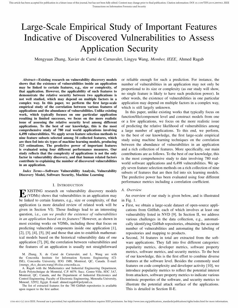
out of one, which is the biggest proportion), so we increase thescore by 2× 1/1. This step takes into account names that arerelated as they share a common part, but are further apart. Weshow in Fig. 2 how these two points could be misleading whenthe application names are abbreviated in certain cases only.
We reproduce the same schema on the product’s name com-pared to the repository’s name; however, we strip any dashes,underscores and digits when comparing the whole names, asthose are mostly noisy characters. Also, we attribute 5 pointsinstead of 4 if the names agree with a small edit distance,which gives more importance to matching product/repositorynames than a matching organization. Moreover, we give anextra point if the product and repository names are exactlythe same. This helps to break ties when very similar namesget high scores, e.g., openssl vs. openssh. Finally, if the scoreis non-zero, we check whether the organization and productnames are the same (considering the same edit distance andLCS criteria), e.g., phpbb:phpbb3. We give 2 additional pointsin this case since such names tend to match official products,by contrast to forks that carry a different organization name.The final score is rounded to the nearest integer. The maximumscore is 12.
Products that get a score higher or equal to 5 are consideredbest matches. This threshold takes into consideration productsthat either receive 5 points directly thanks to a fully matchingproduct/repository name, or by a combination of various levelsof matching product vs. repository and owner vs. organizationnames, and/or benefit from the 2-point bonus for similarproduct and repository names. In any case, if such a productexists, it is strongly possible that it is the right one. At the sametime, the threshold is low enough to capture products with e.g.,owner/organization names that match partially (2 points), anda loosely comparable product/repository (3 points). Setting ahigher threshold may miss some loosely related names, whilesetting it lower would encompass more unrelated names andyield many false positives.
2) Heuristics: Some situations can be resolved automati-cally. For instance, if a repository is assigned only one productacross all its CVEs and this product is a best match, then wemap the repository with this product and combine the CVEs.Also, if considering the CVEs attached to all the affectedproducts does not make a difference from simply countingthe occurrences of the GitHub repository being referred asthe official one, then we stop the product mapping and output#CVEs. We also ignore repositories that specify the keyword“mirror” in their description, as such repositories do not liveon GitHub and therefore the popularity metrics we can extractmay be unreliable.
We force manual inspection on any repository that hasfewer than 5 stars, no fork, and consists of 15 files orfewer. Such metrics indicate an unpopular repository thatmight not be an official application repository. For otherrepositories, the scoring system helps us to decide quicklyamong the best matched products. Among the 890 repos-itories we considered, 468 were labeled automatically, 21were discarded as mirrors, 50 were removed due to: beingdeprecated (e.g., horde/horde), vulnerability finder or exploitgenerator (e.g., rapid7/metasploit-framework), PoC/advisories
4
1556-6013 (c) 2018 IEEE. Personal use is permitted, but republication/redistribution requires IEEE permission. See http://www.ieee.org/publications_standards/publications/rights/index.html for more information.
This article has been accepted for publication in a future issue of this journal, but has not been fully edited. Content may change prior to final publication. Citation information: DOI 10.1109/TIFS.2019.2895963, IEEETransactions on Information Forensics and Security
not caught by the previous filter (e.g., Ha0Team/crash-of-sqlite3), non-software, e.g., PDF, papers, documentation, web-sites (e.g., nonce-disrespect/nonce-disrespect), manually la-beled mirrors/read-only repositories (e.g., LibreOffice/core), orempty repositories. Then, 27 repositories were ignored due tothe complexity of properly counting their number of CVE.This happened when repositories are part of bigger projects,or a project spans on multiple repositories and CVEs do notlabel the specific affected repository, as well as in the caseof forked companies, e.g., ownCloud and nextCloud. Furtherwork is required to take such cases into account. Finally,four repositories were discarded since we could not obtainall metrics. In total, we assigned a more accurate #CVEs andwe further consider 788 repositories.
D. Example
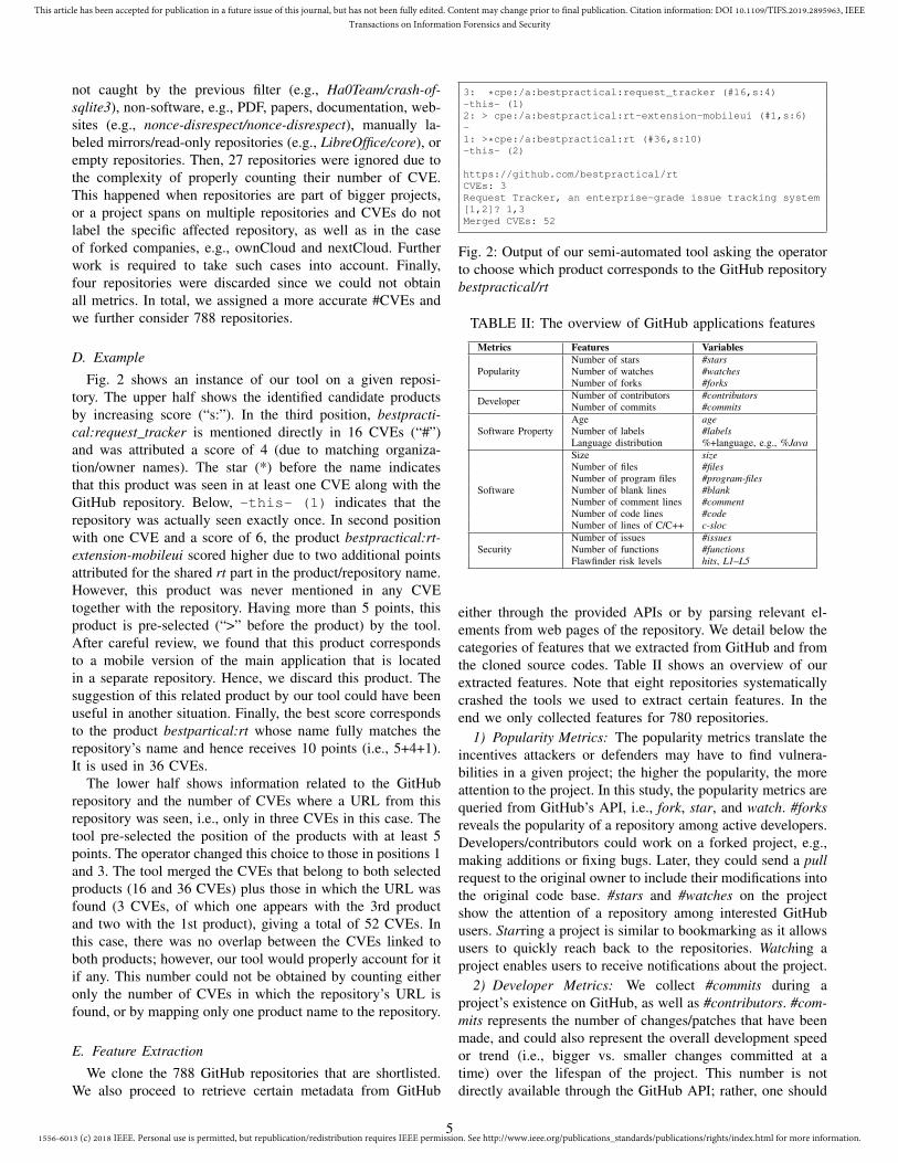
Fig. 2 shows an instance of our tool on a given reposi-tory. The upper half shows the identified candidate productsby increasing score (“s:”). In the third position, bestpracti-cal:request_tracker is mentioned directly in 16 CVEs (“#”)and was attributed a score of 4 (due to matching organiza-tion/owner names). The star (*) before the name indicatesthat this product was seen in at least one CVE along with theGitHub repository. Below, -this- (1) indicates that therepository was actually seen exactly once. In second positionwith one CVE and a score of 6, the product bestpractical:rt-extension-mobileui scored higher due to two additional pointsattributed for the shared rt part in the product/repository name.However, this product was never mentioned in any CVEtogether with the repository. Having more than 5 points, thisproduct is pre-selected (“>” before the product) by the tool.After careful review, we found that this product correspondsto a mobile version of the main application that is locatedin a separate repository. Hence, we discard this product. Thesuggestion of this related product by our tool could have beenuseful in another situation. Finally, the best score correspondsto the product bestpartical:rt whose name fully matches therepository’s name and hence receives 10 points (i.e., 5+4+1).It is used in 36 CVEs.
The lower half shows information related to the GitHubrepository and the number of CVEs where a URL from thisrepository was seen, i.e., only in three CVEs in this case. Thetool pre-selected the position of the products with at least 5points. The operator changed this choice to those in positions 1and 3. The tool merged the CVEs that belong to both selectedproducts (16 and 36 CVEs) plus those in which the URL wasfound (3 CVEs, of which one appears with the 3rd productand two with the 1st product), giving a total of 52 CVEs. Inthis case, there was no overlap between the CVEs linked toboth products; however, our tool would properly account for itif any. This number could not be obtained by counting eitheronly the number of CVEs in which the repository’s URL isfound, or by mapping only one product name to the repository.
E. Feature Extraction
We clone the 788 GitHub repositories that are shortlisted.We also proceed to retrieve certain metadata from GitHub
3: *cpe:/a:bestpractical:request_tracker (#16,s:4)-this- (1)2: > cpe:/a:bestpractical:rt-extension-mobileui (#1,s:6)-1: >*cpe:/a:bestpractical:rt (#36,s:10)-this- (2)
https://github.com/bestpractical/rtCVEs: 3Request Tracker, an enterprise-grade issue tracking system[1,2]? 1,3Merged CVEs: 52
Fig. 2: Output of our semi-automated tool asking the operatorto choose which product corresponds to the GitHub repositorybestpractical/rt
TABLE II: The overview of GitHub applications features
Metrics Features Variables
PopularityNumber of stars #starsNumber of watches #watchesNumber of forks #forks
Developer Number of contributors #contributorsNumber of commits #commits
Software PropertyAge ageNumber of labels #labelsLanguage distribution %+language, e.g., %Java
Software
Size sizeNumber of files #filesNumber of program files #program-filesNumber of blank lines #blankNumber of comment lines #commentNumber of code lines #codeNumber of lines of C/C++ c-sloc
SecurityNumber of issues #issuesNumber of functions #functionsFlawfinder risk levels hits, L1–L5
either through the provided APIs or by parsing relevant el-ements from web pages of the repository. We detail below thecategories of features that we extracted from GitHub and fromthe cloned source codes. Table II shows an overview of ourextracted features. Note that eight repositories systematicallycrashed the tools we used to extract certain features. In theend we only collected features for 780 repositories.
1) Popularity Metrics: The popularity metrics translate theincentives attackers or defenders may have to find vulnera-bilities in a given project; the higher the popularity, the moreattention to the project. In this study, the popularity metrics arequeried from GitHub’s API, i.e., fork, star, and watch. #forksreveals the popularity of a repository among active developers.Developers/contributors could work on a forked project, e.g.,making additions or fixing bugs. Later, they could send a pullrequest to the original owner to include their modifications intothe original code base. #stars and #watches on the projectshow the attention of a repository among interested GitHubusers. Starring a project is similar to bookmarking as it allowsusers to quickly reach back to the repositories. Watching aproject enables users to receive notifications about the project.
2) Developer Metrics: We collect #commits during aproject’s existence on GitHub, as well as #contributors. #com-mits represents the number of changes/patches that have beenmade, and could also represent the overall development speedor trend (i.e., bigger vs. smaller changes committed at atime) over the lifespan of the project. This number is notdirectly available through the GitHub API; rather, one should
5
1556-6013 (c) 2018 IEEE. Personal use is permitted, but republication/redistribution requires IEEE permission. See http://www.ieee.org/publications_standards/publications/rights/index.html for more information.
This article has been accepted for publication in a future issue of this journal, but has not been fully edited. Content may change prior to final publication. Citation information: DOI 10.1109/TIFS.2019.2895963, IEEETransactions on Information Forensics and Security
query the metadata of all commits and count them, generatingseveral hundreds or thousands of queries. Instead, we querythe GitHub repository web page and parse #commits shown.
#contributors may relate to the size of a project in termsof manpower. It could also highlight open-source projectsthat accept various inputs from other developers, which couldtranslate into varying levels of scrutiny on each contribution.We obtain this number through the GitHub API.
3) Software Property Metrics: We consider the creationdate of a repository, which we translate to an age in daysrelative to the day we collected other time-dependent featuresin November 2017. Arguably, the age of a project is expectedto make a difference in #CVEs that have been discovered, asit reflects the exposure period of the application, i.e., the timeanyone has to see the source code, study the application, anddiscover vulnerabilities.
We also consider the relative percentage of each program-ming language in a repository, calculated based on the summedfile sizes corresponding to each language. This distribution isuseful considering the diversity of applications within scopeas it puts the number of lines of code into perspective. Indeed,ten lines of Python arguably carry a different amount ofinformation than ten lines of C, due to Python being a higher-level language. Up to 162 languages are reported by the APIin our study; however, we only consider the 12 most commonones encountered in the repositories: C, C++, C#, Go, HTML,Java, JavaScript, Perl, PHP, Python, Ruby, and Shell, to limitthe dimension of the features.
Finally, we consider the topics assigned to the repository bythe owner. Topics are labels that usually reflect the purpose,subject area, functionalities, community and language of therepository. Examples include “cloud”, “design”, “ecommerce”,“framework”, “packet-capture”, “exploitation”, “windows”,“forum”, “php.” Due to the wide variety of topics and thelack of a proper hierarchical structure to group related topics,we limit our use of topics in this study to their number. Arepository that is labeled with several topics may serve multi-ple purposes and touch several areas, giving some indicationsabout its source code. We refer to this feature as #labels.
4) Software Metrics: The software metrics we collectedfrom the source code cover four levels of granularity: overallprogram size, #files, number of program files (#program-files),and the source lines of code (#code, an estimation for thecyclomatic complexity [13]).
To measure a project’s size, one option is to rely onthe GitHub API, which provides a size parameter for eachrepository. However, the reported size reflects the server-side storage requirement for all revisions with certain storageoptimization. Thus, we resort to cloning all projects locallyand measure only the size of the HEAD tree, i.e., the view ofthe latest revision’s files tree. All projects occupy a total of106GiB on disk, while the API reported only 73.5GiB. Thetotal size representing all latest revisions is 31GiB. The sizeon disk seems to represent the one reported by the API plusthe space taken by the current view of the tree.
#files is obtained by git ls-files, which lists files underthe current repository exhaustively. We use cloc [14] to re-port #code, #blank and #comment in multiple programming
languages. In total, the time effort spent on gathering thosefeatures from the 780 code repositories is 1.5 days. In ad-dition, we also ran Flawfinder [15] to gather C/C++ specificinformation, in particular the number of lines of C/C++ code,referred as c-sloc.
5) Security Metrics: Security metrics that we choose in thisstudy represent two security perspectives: the potential attacklikelihood, and the existing attack likelihood. We use the num-ber of flaws that could be identified by Flawfinder, a widelyused source code auditing tool [6], [15], as the potential attacklikelihood for an application. Flawfinder identifies potentialflaws inside C/C++ source code and outputs the total numberof flaws along with a breakdown according to five severitylevels, e.g, L1 corresponds to the number of flaws with a level1 severity (the lowest).
To quantify the potential threats in an application, weleverage the attack surface [16], which is defined as thesum of entry/exit points (i.e., the functions directly/indirectlyinvoking I/O functions). However, to obtain the attack surface,we would need to construct call graphs for all applications,which is not necessary trivial to establish. Therefore, weconsider the number of functions, which is the upper bound ofthe attack surface metric, as the approximation of the attacksurface metric to indicate the potential attack likelihood. Thesummation of the functions was indexed by C-tag.4
The number of issues on a project reflects software bugsreported by users and also list tasks for project maintainers.Certain issues are related to security, e.g., issue #6599 inopenssl, a bug related to accepting invalid certificate versions,5
which could lead to security vulnerabilities. In this study, thenumber of issues on a project is considered as an indicator ofthe existing attack likelihood.
III. FEATURE SELECTION
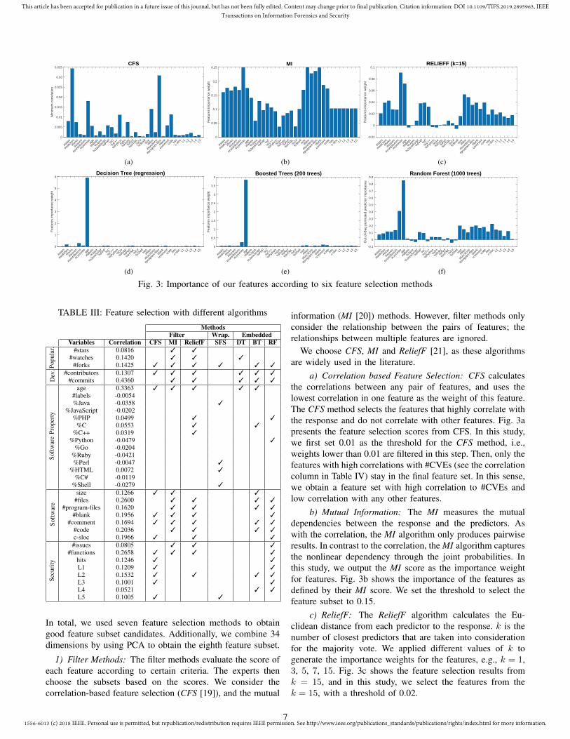
In this section, we apply machine learning techniques on ourfeature set to remove noisy and correlated features to the targetvariable, #CVEs. All the experiments are built with MATLAB.We uniformize the terms used in the latter sections. We referto the target variable in regression models as response and thefeatures in regression models are referred as predictors. Thedata entries are referred to as observations in all the models.Table III summarizes the feature selection results.
A. Feature Selection
A commonly known effect in machine learning, curse ofdimensionality, points out that an increasing feature spacedimensionality weakens the reliability of trained analysissystems [17] by overfitting the data. An efficient solutionis to apply feature selection to find feature subsets, withlower-dimensional space, which leads to more reliable learningresults. Feature selection is also known to enhance the pre-diction performance, lower the computational costs, simplifythe models and provides better understanding in the learningproblems [18]. We use three types of feature selection meth-ods: filter methods, wrapper methods, and embedded methods.
4http://bxr.su/FreeBSD/usr.bin/ctags/5https://github.com/openssl/openssl/issues/6599
6
1556-6013 (c) 2018 IEEE. Personal use is permitted, but republication/redistribution requires IEEE permission. See http://www.ieee.org/publications_standards/publications/rights/index.html for more information.
This article has been accepted for publication in a future issue of this journal, but has not been fully edited. Content may change prior to final publication. Citation information: DOI 10.1109/TIFS.2019.2895963, IEEETransactions on Information Forensics and Security
CFS
#sta
rs
#wat
ches
#for
ks
#issu
es
#con
tribu
tors
#com
mits ag
e
#labe
ls
%Ja
va
%Ja
vaScr
ipt
%PHP
%C
%C++
%Pyth
on%
Go
%Rub
y
%Per
l
%HTM
L%
C#
%She
llsiz
e#f
iles
#fun
ction
s
#pro
gram
-filesbla
nk
com
men
tco
de hits
c-slo
c L1 L2 L3 L4 L50
0.005
0.01
0.015
0.02
0.025
0.03
0.035
Min
imum
cor
rela
tion
(a)
MI
#sta
rs
#wat
ches
#for
ks
#issu
es
#con
tribu
tors
#com
mits ag
e
#labe
ls
%Ja
va
%Ja
vaScr
ipt
%PHP
%C
%C++
%Pyth
on%
Go
%Rub
y
%Per
l
%HTM
L%
C#
%She
llsiz
e#f
iles
#fun
ction
s
#pro
gram
-filesbla
nk
com
men
tco
de hits
c-slo
c L1 L2 L3 L4 L50
0.05
0.1
0.15
0.2
0.25
Fea
ture
s im
port
ance
wei
ght
(b)
RELIEFF (k=15)
#sta
rs
#wat
ches
#for
ks
#issu
es
#con
tribu
tors
#com
mits ag
e
#labe
ls
%Ja
va
%Ja
vaScr
ipt
%PHP
%C
%C++
%Pyth
on%
Go
%Rub
y
%Per
l
%HTM
L%
C#
%She
llsiz
e#f
iles
#fun
ction
s
#pro
gram
-filesbla
nk
com
men
tco
de hits
c-slo
c L1 L2 L3 L4 L5-0.02
0
0.02
0.04
0.06
0.08
0.1
Fea
ture
s im
port
ance
wei
ght
(c)Decision Tree (regression)
#sta
rs
#wat
ches
#for
ks
#issu
es
#con
tribu
tors
#com
mits ag
e
#labe
ls
%Ja
va
%Ja
vaScr
ipt
%PHP
%C
%C++
%Pyth
on%
Go
%Rub
y
%Per
l
%HTM
L%
C#
%She
llsiz
e#f
iles
#fun
ction
s
#pro
gram
-files
blank
com
men
tco
de hits
c-slo
c L1 L2 L3 L4 L50
1
2
3
4
5
6
Fea
ture
s im
port
ance
wei
ght
(d)
Boosted Trees (200 trees)
#sta
rs
#wat
ches
#for
ks
#issu
es
#con
tribu
tors
#com
mits ag
e
#labe
ls
%Ja
va
%Ja
vaScr
ipt
%PHP
%C
%C++
%Pyth
on%
Go
%Rub
y
%Per
l
%HTM
L%
C#
%She
llsiz
e#f
iles
#fun
ction
s
#pro
gram
-files
blank
com
men
tco
de hits
c-slo
c L1 L2 L3 L4 L50
0.5
1
1.5
2
2.5
3
3.5
4
Fea
ture
s im
port
ance
wei
ght
(e)
Random Forest (1000 trees)
#sta
rs
#wat
ches
#for
ks
#issu
es
#con
tribu
tors
#com
mits ag
e
#labe
ls
%Ja
va
%Ja
vaScr
ipt
%PHP
%C
%C++
%Pyth
on%
Go
%Rub
y
%Per
l
%HTM
L%
C#
%She
llsiz
e#f
iles
#fun
ction
s
#pro
gram
-files
blank
com
men
tco
de hits
c-slo
c L1 L2 L3 L4 L5-0.1
0
0.1
0.2
0.3
0.4
0.5
0.6
0.7
0.8
0.9
Out
-of-
Bag
per
mut
ed p
redi
ctor
impo
rtan
ce
(f)
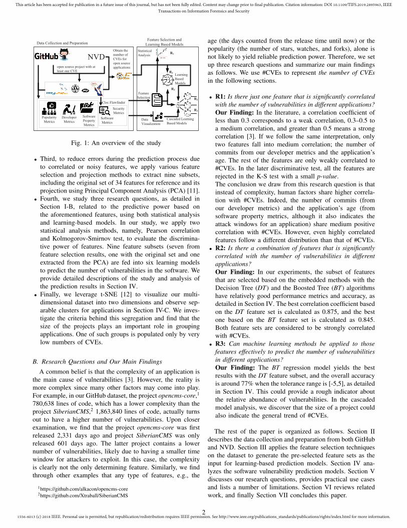
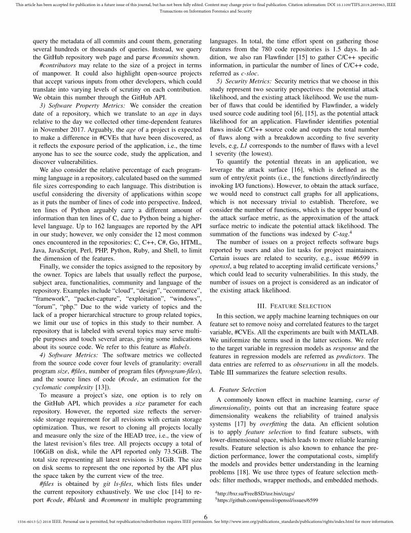
Fig. 3: Importance of our features according to six feature selection methods
TABLE III: Feature selection with different algorithms
MethodsFilter Wrap. Embedded
Variables Correlation CFS MI ReliefF SFS DT BT RF
Popu
lar. #stars 0.0816 3 3
#watches 0.1420 3 3 3#forks 0.1425 3 3 3 3 3 3
De v
. #contributors 0.1307 3 3 3 3 3 3#commits 0.4360 3 3 3 3 3
Soft
war
ePr
oper
ty
age 0.3363 3 3 3 3 3#labels -0.0054%Java -0.0358 3
%JavaScript -0.0202%PHP 0.0499 3 3
%C 0.0553 3 3%C++ 0.0319 3
%Python -0.0479 3%Go -0.0204
%Ruby -0.0421%Perl -0.0047 3
%HTML 0.0072 3%C# -0.0119
%Shell -0.0279 3
Soft
war
e
size 0.1266 3 3 3#files 0.2600 3 3 3 3
#program-files 0.1620 3 3 3 3#blank 0.1956 3 3 3 3
#comment 0.1694 3 3 3 3 3#code 0.2036 3 3 3 3c-sloc 0.1966 3 3 3
Secu
rity
#issues 0.0805 3 3 3#functions 0.2658 3 3 3 3
hits 0.1246 3 3L1 0.1209 3 3L2 0.1532 3 3 3 3L3 0.1001 3 3L4 0.0521 3 3L5 0.1005 3 3
In total, we used seven feature selection methods to obtaingood feature subset candidates. Additionally, we combine 34dimensions by using PCA to obtain the eighth feature subset.
1) Filter Methods: The filter methods evaluate the score ofeach feature according to certain criteria. The experts thenchoose the subsets based on the scores. We consider thecorrelation-based feature selection (CFS [19]), and the mutual
information (MI [20]) methods. However, filter methods onlyconsider the relationship between the pairs of features; therelationships between multiple features are ignored.
We choose CFS, MI and ReliefF [21], as these algorithmsare widely used in the literature.
a) Correlation based Feature Selection: CFS calculatesthe correlations between any pair of features, and uses thelowest correlation in one feature as the weight of this feature.The CFS method selects the features that highly correlate withthe response and do not correlate with other features. Fig. 3apresents the feature selection scores from CFS. In this study,we first set 0.01 as the threshold for the CFS method, i.e.,weights lower than 0.01 are filtered in this step. Then, only thefeatures with high correlations with #CVEs (see the correlationcolumn in Table IV) stay in the final feature set. In this sense,we obtain a feature set with high correlation to #CVEs andlow correlation with any other features.
b) Mutual Information: The MI measures the mutualdependencies between the response and the predictors. Aswith the correlation, the MI algorithm only produces pairwiseresults. In contrast to the correlation, the MI algorithm capturesthe nonlinear dependency through the joint probabilities. Inthis study, we output the MI score as the importance weightfor features. Fig. 3b shows the importance of the features asdefined by their MI score. We set the threshold to select thefeature subset to 0.15.
c) ReliefF: The ReliefF algorithm calculates the Eu-clidean distance from each predictor to the response. k is thenumber of closest predictors that are taken into considerationfor the majority vote. We applied different values of k togenerate the importance weights for the features, e.g., k = 1,3, 5, 7, 15. Fig. 3c shows the feature selection results fromk = 15, and in this study, we select the features from thek = 15, with a threshold of 0.02.
7
1556-6013 (c) 2018 IEEE. Personal use is permitted, but republication/redistribution requires IEEE permission. See http://www.ieee.org/publications_standards/publications/rights/index.html for more information.
This article has been accepted for publication in a future issue of this journal, but has not been fully edited. Content may change prior to final publication. Citation information: DOI 10.1109/TIFS.2019.2895963, IEEETransactions on Information Forensics and Security
2) Wrapper Methods: The wrapper methods involve learn-ing algorithms to evaluate the relevance of the feature sets.Ideally, wrapper methods test all the possible permutations forthe feature subsets and output the ones with the best resultsin terms of accuracy. The corresponding computation timegrows exponentially with the number of features. Heuristicalgorithms, such as the sequential forward selection (SFS),are proposed to tackle this search problem. SFS starts froman empty set and adds features one by one to obtain thebest feature set. We apply the SFS and the sequential forwardfloating selection (SFFS). We only report the result from SFSsince both yield the same results.
3) Embedded Methods: The embedded methods build thelearning algorithms inside the feature selection process, e.g.,decision trees [22], random forests [23]. The selected featureset is generated automatically after the learning process.
We implemented three embedded methods: binary regres-sion decision tree (DT), boosted regression trees using leastsquares boosting (BT), and Random Forest (RF). Fig. 3ddemonstrates the importance weight for each feature fromthe DT method. We choose 0.05 as our threshold; anotherthreshold value might be chosen base on expert knowledge.
The number of trees is the common parameter in boththe BT and RF method; we choose 200, 500, and 1000trees for both methods. During our experiment, changing theparameter’s value only bring negligible differences in thefeature importance weights. We only show the results fromthe BT method with 200 trees in Fig. 3e, and the RF methodwith 1000 trees in Fig. 3f. Based on expert knowledge, wechoose threshold as 0.018 and 0.1, respectively.
IV. ANALYSIS
In this section, we first apply two statistical methods toevaluate the correlations between the features and #CVEs inSection IV-A. Then, the prediction powers of learning-basedmodels are analyzed in Section IV-B. Finally, we conductcascaded model analysis to further study the relationshipsbetween features and #CVEs in Section IV-C.
A. Statistical Analysis
We apply two statistical methods to evaluate the correlationsbetween our features and #CVEs. First, we normalize thefeature sets with Equation 1 (Min-Max standardization) totransfer the values of features to a bounded range.
zi =xi −min(x)
max(x)−min(x)(1)
where x = (x1, . . . , xn) are the original features in the datasetand zi is the ith normalized data. Equation 1 maps the valuesof all features into the same range [0, 1].
The first statistical analysis is the Pearson coefficient, whichillustrates the linear relationships between the response andpredictors, e.g., in our case, the #CVEs and features. Thecorrelation coefficient takes values between -1 to 1, whichcorresponds to a perfect direct decreasing (negative) or in-creasing (positive) linear relationship, respectively. The value0 means that the two input variables are not correlated.
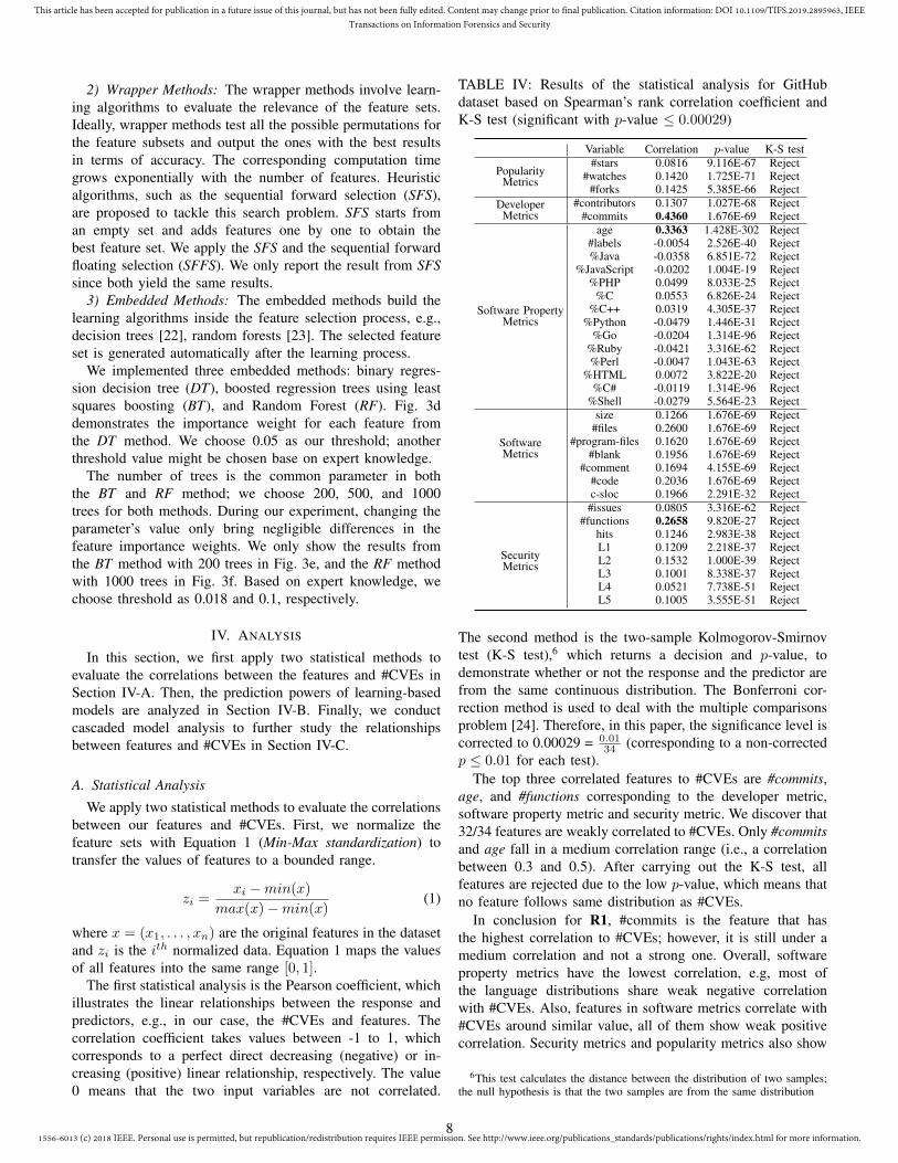
TABLE IV: Results of the statistical analysis for GitHubdataset based on Spearman’s rank correlation coefficient andK-S test (significant with p-value ≤ 0.00029)
Variable Correlation p-value K-S test
PopularityMetrics
#stars 0.0816 9.116E-67 Reject#watches 0.1420 1.725E-71 Reject
#forks 0.1425 5.385E-66 RejectDeveloper
Metrics#contributors 0.1307 1.027E-68 Reject
#commits 0.4360 1.676E-69 Reject
Software PropertyMetrics
age 0.3363 1.428E-302 Reject#labels -0.0054 2.526E-40 Reject%Java -0.0358 6.851E-72 Reject
%JavaScript -0.0202 1.004E-19 Reject%PHP 0.0499 8.033E-25 Reject
%C 0.0553 6.826E-24 Reject%C++ 0.0319 4.305E-37 Reject
%Python -0.0479 1.446E-31 Reject%Go -0.0204 1.314E-96 Reject
%Ruby -0.0421 3.316E-62 Reject%Perl -0.0047 1.043E-63 Reject
%HTML 0.0072 3.822E-20 Reject%C# -0.0119 1.314E-96 Reject
%Shell -0.0279 5.564E-23 Reject
SoftwareMetrics
size 0.1266 1.676E-69 Reject#files 0.2600 1.676E-69 Reject
#program-files 0.1620 1.676E-69 Reject#blank 0.1956 1.676E-69 Reject
#comment 0.1694 4.155E-69 Reject#code 0.2036 1.676E-69 Rejectc-sloc 0.1966 2.291E-32 Reject
SecurityMetrics
#issues 0.0805 3.316E-62 Reject#functions 0.2658 9.820E-27 Reject
hits 0.1246 2.983E-38 RejectL1 0.1209 2.218E-37 RejectL2 0.1532 1.000E-39 RejectL3 0.1001 8.338E-37 RejectL4 0.0521 7.738E-51 RejectL5 0.1005 3.555E-51 Reject
The second method is the two-sample Kolmogorov-Smirnovtest (K-S test),6 which returns a decision and p-value, todemonstrate whether or not the response and the predictor arefrom the same continuous distribution. The Bonferroni cor-rection method is used to deal with the multiple comparisonsproblem [24]. Therefore, in this paper, the significance level iscorrected to 0.00029 = 0.01
34 (corresponding to a non-correctedp ≤ 0.01 for each test).
The top three correlated features to #CVEs are #commits,age, and #functions corresponding to the developer metric,software property metric and security metric. We discover that32/34 features are weakly correlated to #CVEs. Only #commitsand age fall in a medium correlation range (i.e., a correlationbetween 0.3 and 0.5). After carrying out the K-S test, allfeatures are rejected due to the low p-value, which means thatno feature follows same distribution as #CVEs.
In conclusion for R1, #commits is the feature that hasthe highest correlation to #CVEs; however, it is still under amedium correlation and not a strong one. Overall, softwareproperty metrics have the lowest correlation, e.g, most ofthe language distributions share weak negative correlationwith #CVEs. Also, features in software metrics correlate with#CVEs around similar value, all of them show weak positivecorrelation. Security metrics and popularity metrics also show
6This test calculates the distance between the distribution of two samples;the null hypothesis is that the two samples are from the same distribution
8
1556-6013 (c) 2018 IEEE. Personal use is permitted, but republication/redistribution requires IEEE permission. See http://www.ieee.org/publications_standards/publications/rights/index.html for more information.
This article has been accepted for publication in a future issue of this journal, but has not been fully edited. Content may change prior to final publication. Citation information: DOI 10.1109/TIFS.2019.2895963, IEEETransactions on Information Forensics and Security
weak correlations. However, all the features are under differentdistribution with #CVEs.
B. Single-model Learning-based Analysis
1) Experiment Models and Evaluation Methods: Unlikesome existing works, which focus on vulnerability discoveryat the file level within an application and with a binary output(i.e., vulnerable or not), this study leverages regression modelswith which responses are numeric values that correspond to#CVEs per application. We conducted this experiment usingsix regression models with various parameters on differentsets of features, totaling 523 prediction results. We refer asfeature-selection-method set the feature subset generated fromthe feature-selection-method, e.g., DT set.Data Preparation. 240 out of 780 projects contain at least50% of C/C++, and up to 302 contain any proportion of C/C++in our dataset. As Flawfinder only supports C/C++ projects,we assign the value -1 to all Flawfinder-related features(expectedly positive integers) for projects with a zero amountof C/C++ according to the GitHub repository’s metadata [25].Performance metrics. The performance of a learning model isevaluated through root mean squared error (RMSE), a widelyused measure of error that emphasizes large errors; meanabsolute error (MAE), which measures the absolute differencebetween predicted values and responses; and mean absolutepercentage error (MAPE) that gives a relative measure ofdiscrepancies and also gives more emphasis on errors for small#CVEs. Usually, a lower rate of errors corresponds to betterperformance of a model for a given feature set. In addition,correlation is used to compare the trend between responsesand predictors. In Table VI, the best feature sets are chosenbased on the criteria given below.Boosted Tree. We leveraged boosted regression trees usingleast squares boosting, BT and BT-opt. BT-opt is selectedto calculate parameters with the inbuilt algorithms. Table Vdemonstrates the evaluation results of RMSE, MAE andMAPE. The prediction results from BT-opt with all featureshas the lowest MAPE; however, the RMSE and MAE arehigher than BT with the DT set. The main reason for thisobservation is that evaluation methods are more sensitive tocapturing errors in certain types of data. For example, MAPEis sensitive to the errors from small values inside one datasetwhile RMSE captures the existence of large errors resultingfrom the prediction.Decision Tree for Regression. In the DT model, the MI setyields the best MAE; however, the BT set has the best RMSEand MAPE. Therefore, the prediction results from DT withBT set are presented in Table VI and Fig. 4b. The accuracyof the predicted results are presented in Fig. 5b.Linear Regression. In the LR model, the DT set has thebest RMSE. The SFS set has the best MAE and MAPE.The correlation is calculated as 0.451 and 0.434 from thepredictions, respectively; therefore, we only demonstrate thebest results from DT set in Table VI and show the predictedresults and the accuracy in Fig. 4c and Fig. 5c.Neural Networks. We apply two Neural Network (NN) mod-els, function fitting NN (FFNN) and generalized regression NN
(GRNN). To obtain relatively better results from both models,we choose 36 hidden layers (from 1 to 36) to get the bestRMSE, MAE and MAPE for different feature sets. The BT setwith 4 hidden layers obtains the best RMSE, and the DT setwith 6 hidden layers obtains the best MAE and MAPE in theFFNN model, which is overall better than the GRNN model.Since the correlation is 0.533 for the BT set, which is higherthan the correlation from the DT set, 0.406, we only show theresult of the BT set in Table VI and show the predicted resultsand the accuracy in Fig. 4d and Fig. 5d.Random Forest. We consider the RF model with variousnumber of trees, 10, 100, 200, 500 and 1000. The best resultis obtained from the DT set with 500 trees, and is presentedin Table VI, Fig. 4e and Fig. 5e.Support Vector Machine Regression. We leverage SupportVector Machine Regression (SVR) with three different solvers,i.e., ISDA, L1QP, and SMO solver, and with three kernels, i.e.,Gaussian, Linear and Polynomial. The best overall predictiveresults are generated from the ISDA solver with the Gaussiankernel with the DT set; see Table VI. However, the SVR modelalso yields the lowest MAPE (66.61%) with the L1QP solverand polynomial kernel using the CFS set. We list the predictionresults of the CFS set corresponding to the accuracy in Fig. 4fand Fig. 5f.Cross-validation. Each of the training and prediction experi-ments has been conducted using ten-fold cross-validation [26].The same randomized folds are used with the linear, NN, andRF models (i.e., we perform 10 training-prediction segmentsbased on the randomly pre-separated folds, and average theresults), while folds for the BT, DT, and SVR models areselected internally in MATLAB.
For the NN model, a validation set is also used to avoidoverfitting [27]. We randomly split each training set (repre-senting 90% of our data) into 9 parts and use one as thevalidation set, giving 80%, 10%, 10% for training, testing,and validation, respectively. These proportions are on par withMATLAB default’s, i.e., 70%, 15%, 15% [27], but match moreclosely the proportions of a classic ten-fold cross-validation.
2) Experiment Results Interpretation: The DT set, whichonly contains four features from three categories, providesthe best evaluation results for five models. It contains themost generic features, thus it discards all the applicationcode specific features. This result indicates that the generalcomparison among applications could simply be generatedfrom developers, popularity and the existing time of theapplications. The BT set, which involves more software andsecurity metrics, perform similarly to the DT set.
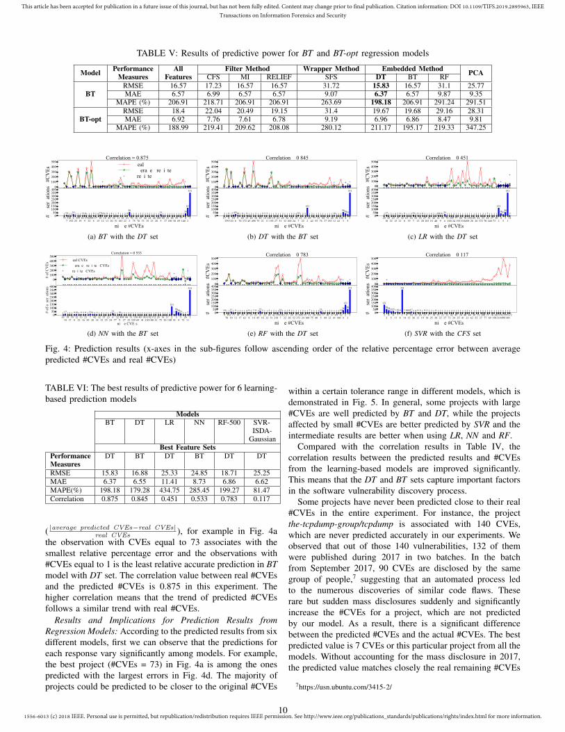
To better understand the prediction results, Fig. 4 sum-marizes the predicted value from the best models and thefeature sets. Since multiple observations correspond to thesame #CVEs in our dataset, we group the observations basedon #CVEs. X-axes in the graphs represent bins of unique#CVEs. The red squares in the upper graph plot the real#CVEs for each unique #CVEs, which are the same asthe labels on the x-axis. The green crosses are the aver-age predicted #CVEs for each unique #CVEs and the bluepluses are the predicted #CVEs for each observation. Thepredicted results are ordered by the relative percentage error
9
1556-6013 (c) 2018 IEEE. Personal use is permitted, but republication/redistribution requires IEEE permission. See http://www.ieee.org/publications_standards/publications/rights/index.html for more information.
This article has been accepted for publication in a future issue of this journal, but has not been fully edited. Content may change prior to final publication. Citation information: DOI 10.1109/TIFS.2019.2895963, IEEETransactions on Information Forensics and Security
TABLE V: Results of predictive power for BT and BT-opt regression models
Model Performance All Filter Method Wrapper Method Embedded Method PCAMeasures Features CFS MI RELIEF SFS DT BT RF
BTRMSE 16.57 17.23 16.57 16.57 31.72 15.83 16.57 31.1 25.77MAE 6.57 6.99 6.57 6.57 9.07 6.37 6.57 9.87 9.35
MAPE (%) 206.91 218.71 206.91 206.91 263.69 198.18 206.91 291.24 291.51
BT-optRMSE 18.4 22.04 20.49 19.15 31.4 19.67 19.68 29.16 28.31MAE 6.92 7.76 7.61 6.78 9.19 6.96 6.86 8.47 9.81
MAPE (%) 188.99 219.41 209.62 208.08 280.12 211.17 195.17 219.33 347.25
�������
�����
����
���
�����
�������������������������
�����
���������������������
���������
����������
���
����������������
����"
��!!���#���� ����������%�!�����!����#���!����#��
�������
�����
����
���
�����
�������������������������
�����
���������������������
���������
����������
���
��� $������"
������������������������
���"�!%�#��
�"
��� ���� � � ��� � � � � ����� � � � � � � � � ��
� � � � � � � � � � � � ���� � � � � � � � � ���
���
���
(a) BT with the DT set
����
����
��
��
����
����
����
��
����
����
������
���
���
����
�����
����
��
����
���
���
��
��
���
����
����
����
����
��
��
���������������
���
��
������������ ������
����
����
��
��
����
����
����
��
����
����
������
���
���
����
�����
����
��
����
���
���
��
��
���
����
����
����
����
��
�
������������
���
���������������������
����
����
�����
� � � ������� � � � � � � � � � � � � � � � � � � � � � � ��� � �
���
� � � � � � � � � � ���� � ������
���
(b) DT with the BT set
����
����
����
���
���
���
�
����
����
����
����
����
���
��
����
�����
���
�����
���
�����
��
����
���
�����
��
���
��
��
���
���������������
���
��
������������ ������
����
����
����
���
���
���
�
����
����
����
����
����
���
��
����
�����
���
�����
���
�����
��
����
���
�����
��
���
��
��
��
������������
���
���������������������
����
����
�����
��� � � � � � � � � � ��� � � � � � � � � ��������� � � � � � � � � � � � � � � � � � � � � �
���
�����
���
(c) LR with the DT set
����������
����������
����� �������
����
��
��������
����� �������������
��� ���������
��
�������
�
��������������
��!�����$
�!##���%�! �������
��������$�'�#�����#����%������$�#����%������$
����������
����������
����� �������
����
��
��������
����� �������������
��� ���������
��
�������
�
� �"&������$�
�������������������
��!��!�$�#'�%�!
$
���� � � ���� � � ��� � � � � � ��� ���� � � � � � � � � � � � � � � � � � � � � �
���
��� ��� � �
��
(d) NN with the BT set
��
�����
���
���
�
���
����
����
�
����
����
�����
������
���
���
����
�����
����
�����
���
�����
�
����
���
���
�����
��
��
����������������
���
��
������������ �����
��
�����
���
���
�
���
����
����
�
����
����
�����
������
���
���
����
�����
����
�����
���
�����
�
����
���
���
�����
��
��
������������
���
���������������������
����
����
�����
��� ��� � � � � � � � � � ���� � � � � � � ��� � � � � � � � � � � � � � � ���� � � � � � � �����
����
���
(e) RF with the DT set
��
��
��
�
���
���
���
����
���
����
���
���
����
���
���
����
����
����
����
���
����
���
���
��
���
������
������
������
���
���������������
���
��
������������ �����
��
��
��
�
���
���
���
����
���
����
���
���
����
���
���
����
����
����
����
���
����
���
���
��
���
������
������
������
��
������������
���
���������������������
����
����
�����
������������
���
������ � � � � � � � � � � � � � � � � � � � � � � � � � � � � � � � � � � � � � � � � � � �
(f) SVR with the CFS set
Fig. 4: Prediction results (x-axes in the sub-figures follow ascending order of the relative percentage error between averagepredicted #CVEs and real #CVEs)
TABLE VI: The best results of predictive power for 6 learning-based prediction models
ModelsBT DT LR NN RF-500 SVR-
ISDA-Gaussian
Best Feature SetsPerformanceMeasures
DT BT DT BT DT DT
RMSE 15.83 16.88 25.33 24.85 18.71 25.25MAE 6.37 6.55 11.41 8.73 6.86 6.62MAPE(%) 198.18 179.28 434.75 285.45 199.27 81.47Correlation 0.875 0.845 0.451 0.533 0.783 0.117
( |average predicted CVEs−real CVEs|real CVEs ), for example in Fig. 4a
the observation with CVEs equal to 73 associates with thesmallest relative percentage error and the observations with#CVEs equal to 1 is the least relative accurate prediction in BTmodel with DT set. The correlation value between real #CVEsand the predicted #CVEs is 0.875 in this experiment. Thehigher correlation means that the trend of predicted #CVEsfollows a similar trend with real #CVEs.
Results and Implications for Prediction Results fromRegression Models: According to the predicted results from sixdifferent models, first we can observe that the predictions foreach response vary significantly among models. For example,the best project (#CVEs = 73) in Fig. 4a is among the onespredicted with the largest errors in Fig. 4d. The majority ofprojects could be predicted to be closer to the original #CVEs
within a certain tolerance range in different models, which isdemonstrated in Fig. 5. In general, some projects with large#CVEs are well predicted by BT and DT, while the projectsaffected by small #CVEs are better predicted by SVR and theintermediate results are better when using LR, NN and RF.
Compared with the correlation results in Table IV, thecorrelation results between the predicted results and #CVEsfrom the learning-based models are improved significantly.This means that the DT and BT sets capture important factorsin the software vulnerability discovery process.
Some projects have never been predicted close to their real#CVEs in the entire experiment. For instance, the projectthe-tcpdump-group/tcpdump is associated with 140 CVEs,which are never predicted accurately in our experiments. Weobserved that out of those 140 vulnerabilities, 132 of themwere published during 2017 in two batches. In the batchfrom September 2017, 90 CVEs are disclosed by the samegroup of people,7 suggesting that an automated process ledto the numerous discoveries of similar code flaws. Theserare but sudden mass disclosures suddenly and significantlyincrease the #CVEs for a project, which are not predictedby our model. As a result, there is a significant differencebetween the predicted #CVEs and the actual #CVEs. The bestpredicted value is 7 CVEs or this particular project from all themodels. Without accounting for the mass disclosure in 2017,the predicted value matches closely the real remaining #CVEs
7https://usn.ubuntu.com/3415-2/
10
1556-6013 (c) 2018 IEEE. Personal use is permitted, but republication/redistribution requires IEEE permission. See http://www.ieee.org/publications_standards/publications/rights/index.html for more information.
This article has been accepted for publication in a future issue of this journal, but has not been fully edited. Content may change prior to final publication. Citation information: DOI 10.1109/TIFS.2019.2895963, IEEETransactions on Information Forensics and Security
������� ������� ������� ������� ��������������!��������
������������������������
���
"���
$
���������� ������� ����
��� �����#�����
(a) BT with the DT set
������� ������� ������� ������� ��������������!��������
���
���
���
���
��
��
���
���
��
���
"���
$
���������� ������� ����
��� �����#�����
(b) DT with the BT set
������� ������� ������� ������� ��������������!��������
������������������������
���
"���
$
���������� ������� ����
��� �����#�����
(c) LR with the DT set
������� ������� ������� ������� ��������������!��������
���
���
���
���
��
��
���
���
�� ���
"���
$
���������� ������� ����
��� �����#�����
(d) NN with the BT set
������� ������� ������� ������� ��������������!��������
���
���
���
���
��
��
���
���
��
���
"���
$
���������� ������� ����
��� �����#�����
(e) RF with the DT set
������� ������� ������� ������� ��������������!��������
������������������������
���
"���
$
���������� ������� ����
��� �����#�����
(f) SVR with the CFS set
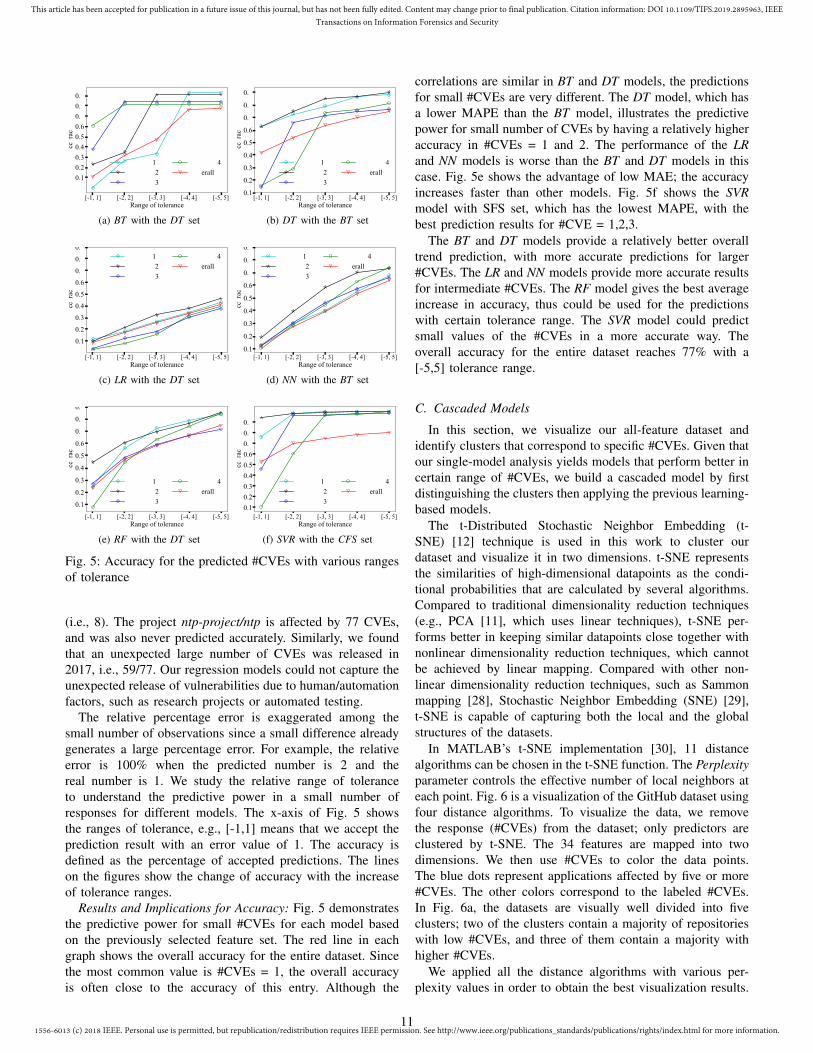
Fig. 5: Accuracy for the predicted #CVEs with various rangesof tolerance
(i.e., 8). The project ntp-project/ntp is affected by 77 CVEs,and was also never predicted accurately. Similarly, we foundthat an unexpected large number of CVEs was released in2017, i.e., 59/77. Our regression models could not capture theunexpected release of vulnerabilities due to human/automationfactors, such as research projects or automated testing.
The relative percentage error is exaggerated among thesmall number of observations since a small difference alreadygenerates a large percentage error. For example, the relativeerror is 100% when the predicted number is 2 and thereal number is 1. We study the relative range of toleranceto understand the predictive power in a small number ofresponses for different models. The x-axis of Fig. 5 showsthe ranges of tolerance, e.g., [-1,1] means that we accept theprediction result with an error value of 1. The accuracy isdefined as the percentage of accepted predictions. The lineson the figures show the change of accuracy with the increaseof tolerance ranges.
Results and Implications for Accuracy: Fig. 5 demonstratesthe predictive power for small #CVEs for each model basedon the previously selected feature set. The red line in eachgraph shows the overall accuracy for the entire dataset. Sincethe most common value is #CVEs = 1, the overall accuracyis often close to the accuracy of this entry. Although the
correlations are similar in BT and DT models, the predictionsfor small #CVEs are very different. The DT model, which hasa lower MAPE than the BT model, illustrates the predictivepower for small number of CVEs by having a relatively higheraccuracy in #CVEs = 1 and 2. The performance of the LRand NN models is worse than the BT and DT models in thiscase. Fig. 5e shows the advantage of low MAE; the accuracyincreases faster than other models. Fig. 5f shows the SVRmodel with SFS set, which has the lowest MAPE, with thebest prediction results for #CVE = 1,2,3.
The BT and DT models provide a relatively better overalltrend prediction, with more accurate predictions for larger#CVEs. The LR and NN models provide more accurate resultsfor intermediate #CVEs. The RF model gives the best averageincrease in accuracy, thus could be used for the predictionswith certain tolerance range. The SVR model could predictsmall values of the #CVEs in a more accurate way. Theoverall accuracy for the entire dataset reaches 77% with a[-5,5] tolerance range.
C. Cascaded Models
In this section, we visualize our all-feature dataset andidentify clusters that correspond to specific #CVEs. Given thatour single-model analysis yields models that perform better incertain range of #CVEs, we build a cascaded model by firstdistinguishing the clusters then applying the previous learning-based models.
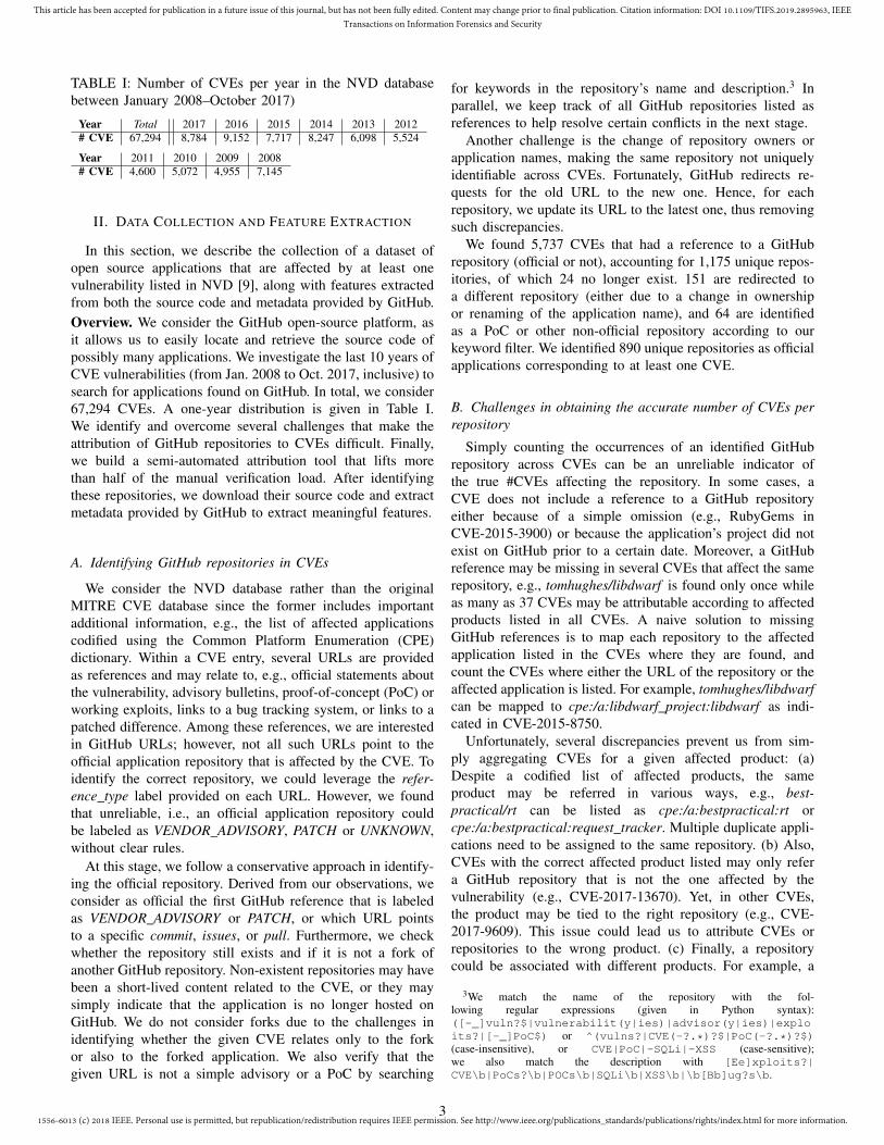
The t-Distributed Stochastic Neighbor Embedding (t-SNE) [12] technique is used in this work to cluster ourdataset and visualize it in two dimensions. t-SNE representsthe similarities of high-dimensional datapoints as the condi-tional probabilities that are calculated by several algorithms.Compared to traditional dimensionality reduction techniques(e.g., PCA [11], which uses linear techniques), t-SNE per-forms better in keeping similar datapoints close together withnonlinear dimensionality reduction techniques, which cannotbe achieved by linear mapping. Compared with other non-linear dimensionality reduction techniques, such as Sammonmapping [28], Stochastic Neighbor Embedding (SNE) [29],t-SNE is capable of capturing both the local and the globalstructures of the datasets.
In MATLAB’s t-SNE implementation [30], 11 distancealgorithms can be chosen in the t-SNE function. The Perplexityparameter controls the effective number of local neighbors ateach point. Fig. 6 is a visualization of the GitHub dataset usingfour distance algorithms. To visualize the data, we removethe response (#CVEs) from the dataset; only predictors areclustered by t-SNE. The 34 features are mapped into twodimensions. We then use #CVEs to color the data points.The blue dots represent applications affected by five or more#CVEs. The other colors correspond to the labeled #CVEs.In Fig. 6a, the datasets are visually well divided into fiveclusters; two of the clusters contain a majority of repositorieswith low #CVEs, and three of them contain a majority withhigher #CVEs.
We applied all the distance algorithms with various per-plexity values in order to obtain the best visualization results.
11
1556-6013 (c) 2018 IEEE. Personal use is permitted, but republication/redistribution requires IEEE permission. See http://www.ieee.org/publications_standards/publications/rights/index.html for more information.
This article has been accepted for publication in a future issue of this journal, but has not been fully edited. Content may change prior to final publication. Citation information: DOI 10.1109/TIFS.2019.2895963, IEEETransactions on Information Forensics and Security
-40 -20 0 20 40-40
-20
0
20
40
12345+
(a) Perplexity=30, Euclidean distance-20 -10 0 10 20 30 40
-20
-10
0
10
20
30
12345+
(b) Perplexity=34, Cosine distance
-40 -20 0 20 40-40
-20
0
20
40
12345+
(c) Perplexity=30, Chebychev dist.-40 -20 0 20 40
-40
-20
0
20
40
Cluster 1
Cluster 2
Cluster 3
12345+
(d) Perplexity=30, Minkowski dist.
Fig. 6: Visualization of our data using t-SNE projections basedon all features, and selected perplexity and distance algorithms
(a)
2
3 1
size<744411
size<3.73782e+07
size>=744411
size>=3.73782e+07
(b)
Fig. 7: Cascaded learning-based model (a), Decision tree toclassify the clusters in Fig. 6d (b)
Fig. 6 shows the most visually separated visualization resultsfrom the GitHub dataset.
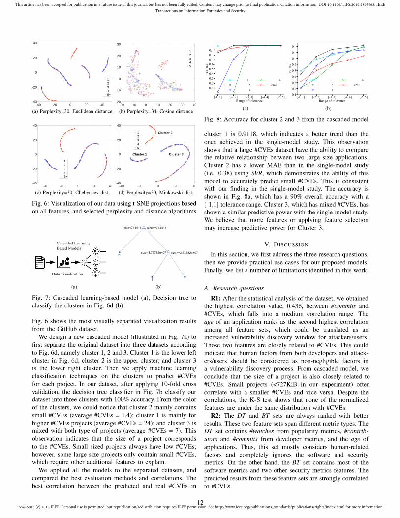
We design a new cascaded model (illustrated in Fig. 7a) tofirst separate the original dataset into three datasets accordingto Fig. 6d, namely cluster 1, 2 and 3. Cluster 1 is the lower leftcluster in Fig. 6d; cluster 2 is the upper cluster; and cluster 3is the lower right cluster. Then we apply machine learningclassification techniques on the clusters to predict #CVEsfor each project. In our dataset, after applying 10-fold crossvalidation, the decision tree classifier in Fig. 7b classify ourdataset into three clusters with 100% accuracy. From the colorof the clusters, we could notice that cluster 2 mainly containssmall #CVEs (average #CVEs = 1.4); cluster 1 is mainly forhigher #CVEs projects (average #CVEs = 24); and cluster 3 ismixed with both type of projects (average #CVEs = 7). Thisobservation indicates that the size of a project correspondsto the #CVEs. Small sized projects always have low #CVEs;however, some large size projects only contain small #CVEs,which require other additional features to explain.
We applied all the models to the separated datasets, andcompared the best evaluation methods and correlations. Thebest correlation between the predicted and real #CVEs in
������� ������� ������� ������� ��������������!��������
������������������������
���
"���
$
���������� ������� ����
��� �����#�����
(a)
������� ������� ������� ������� ��������������!��������
���
���
���
���
��
��
���
���
��
���
"���
$
���������� ������� ����
��� �����#�����
(b)
Fig. 8: Accuracy for cluster 2 and 3 from the cascaded model
cluster 1 is 0.9118, which indicates a better trend than theones achieved in the single-model study. This observationshows that a large #CVEs dataset have the ability to comparethe relative relationship between two large size applications.Cluster 2 has a lower MAE than in the single-model study(i.e., 0.38) using SVR, which demonstrates the ability of thismodel to accurately predict small #CVEs. This is consistentwith our finding in the single-model study. The accuracy isshown in Fig. 8a, which has a 90% overall accuracy with a[-1,1] tolerance range. Cluster 3, which has mixed #CVEs, hasshown a similar predictive power with the single-model study.We believe that more features or applying feature selectionmay increase predictive power for Cluster 3.
V. DISCUSSION
In this section, we first address the three research questions,then we provide practical use cases for our proposed models.Finally, we list a number of limitations identified in this work.
A. Research questions
R1: After the statistical analysis of the dataset, we obtained the highest correlation value, 0.436, between #commits and #CVEs, which falls into a medium correlation range. The age of an application ranks as the second highest correlation among all feature sets, which could be translated as an increased vulnerability discovery window for attackers/users. Those two features are closely related to #CVEs. This could indicate that human factors from both developers and attack-ers/users should be considered as non-negligible factors in a vulnerability discovery process. From cascaded model, we conclude that the size of a project is also closely related to #CVEs. Small projects (<727KiB in our experiment) often correlate with a smaller #CVEs and vice versa. Despite the correlations, the K-S test shows that none of the normalized features are under the same distribution with #CVEs.
R2: The DT and BT sets are always ranked with better results. These two feature sets span different metric types. The DT set contains #watches from popularity metrics, #contrib-utors and #commits from developer metrics, and the age of applications. Thus, this set mostly considers human-related factors and completely ignores the software and security metrics. On the other hand, the BT set contains most of the software metrics and two other security metrics features. The predicted results from these feature sets are strongly correlated to #CVEs.
12
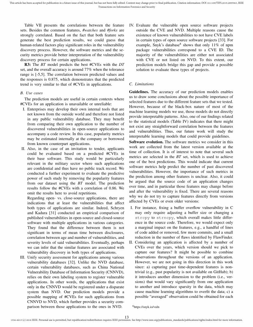
1556-6013 (c) 2018 IEEE. Personal use is permitted, but republication/redistribution requires IEEE permission. See http://www.ieee.org/publications_standards/publications/rights/index.html for more information.
This article has been accepted for publication in a future issue of this journal, but has not been fully edited. Content may change prior to final publication. Citation information: DOI 10.1109/TIFS.2019.2895963, IEEETransactions on Information Forensics and Security
Table VII presents the correlations between the featuresets. Besides the common features, #watches and #forks arestrongly correlated. Based on the fact that both feature setsgenerate the best prediction results, we could guess thathuman-related factors play significant roles in the vulnerabilitydiscovery process. However, the software metrics and the se-curity metrics provide better interpretation of the vulnerabilitydiscovery process for certain applications.
R3: The BT model predicts the best #CVEs with the DTset, and the overall accuracy is around 77% when the tolerancerange is [-5,5]. The correlation between predicted values andthe responses is 0.875, which demonstrates that the predictedtrend is very similar to that of #CVEs in applications.
B. Use casesThe prediction models are useful in certain contexts where
#CVEs for an application is unavailable or unreliable:I. Enterprises may develop their own internal tools that are
not known from the outside world and therefore not listedin any public vulnerability database. They may benefitfrom comparing their own application to the number ofdiscovered vulnerabilities in open-source applications toaccompany a code review. In this case, popularity metricsmay be estimated internally at the company or borrowedfrom known counterpart applications.
II. Also, in the case of an invitation to tender, applicantscould be evaluated based on a predicted #CVEs intheir base software. This study would be particularlyrelevant in the military sector where such applicationsare confidential and thus have no public track record. Weconducted a further experiment to evaluate the predictivepower of such study by removing the popularity featuresfrom our dataset using the BT model. The predictionresults follow the #CVEs with a correlation of 0.86. Weomit the results here to avoid repetitions.Regarding open- vs. close-source applications, there areindications that at least the vulnerabilities that affectboth types of applications are similar. Indeed, Schryenand Kadura [31] conducted an empirical comparison ofpublished vulnerabilities in open-source and closed-sourcesoftware with multiple applications in various categories.They found that the difference between them is notsignificant in terms of mean time between disclosures,correlation between age and number of vulnerabilities, andseverity levels of said vulnerabilities. Eventually, perhapswe can infer that the similar features are associated withvulnerability discovery in both types of applications.
III. Unify security assessment for applications among variousvulnerability databases [32]. Unlike the NVD database,certain vulnerability databases, such as China NationalVulnerability Database of Information Security (CNNVD),relies on their own labeling system to register vulnerableapplications. In other words, the applications that existonly in the CNNVD would be registered under a disparatesystem than NVD. Our prediction models provide apossible mapping of #CVEs for such applications fromCNNVD to NVD, which further provides a security com-parison between those applications to the ones in NVD.
IV. Evaluate the vulnerable open source software projectsoutside the CVE and NVD. Multiple reasons cause theexistence of known vulnerabilities to not have CVE labelsin certain types of open source software projects [33]. Forexample, Snyk’s database8 shows that only 11% of npmpackage vulnerabilities correspond to a CVE ID. Themajority of the vulnerabilities are either not associatedwith CVE or not listed on NVD. To this extent, ourprediction models bridge this gap and provide a possiblesolution to evaluate these types of projects.
C. Limitations
Guidelines. The accuracy of our prediction models enablesus to draw some conclusions about the possible importance ofselected features due to the different feature sets that we tested.However, because of the black-box nature of most of themachine learning models we use, those models do not directlyprovide interpretable patterns. Also, one of our findings relatedto the statistical models (Table IV) indicates that there mightnot exist any straightforward correlation between the featuresand vulnerabilities. Thus, our future work will study theinterpretable learning models that could provide guidelines.Software evolution. The software metrics we consider in thiswork are collected from the latest version available at thetime of collection. It is of interest to note that several suchmetrics are selected in the BT set, which is used to achieveone of the best predictions. This would indicate that currentsoftware metrics help predict the number of past discoveredvulnerabilities. However, the importance of such metrics inthe prediction among other features is unclear. Also, it couldbe argued that the source code of an application changesover time, and in particular those features may change beforeand after the vulnerability is fixed. There are several reasonswhy we do not try to capture features directly from versionsaffected by CVEs or even older versions:
I. For instance, fixing a buffer overflow vulnerability in Cmay only require adjusting a buffer size or changing astrcpy to strncpy, which overall makes little differ-ence in the source code. Therefore, we would expect onlya marginal impact on the features, e.g., a handful of linesof code added or removed, few more commits, and a smallreduction in the number of flaws identified by FlawFinder.
II. Considering an application is affected by a number ofCVEs over the years, which version should we pick tocapture our features? It might be possible to combineobservations throughout the versions of an application.However, we are not going in this direction in this worksince: a) capturing past time-dependent features is non-trivial (e.g., past popularity is not available on GitHub); b)it introduces another dimension to the problem (i.e., ver-sions) that would vary significantly from one applicationto another and introduce sparsity in the data, which maycause machine learning algorithms to overfit the data; c) apossible “averaged” observation could be obtained for each
8https://snyk.io/vuln
13
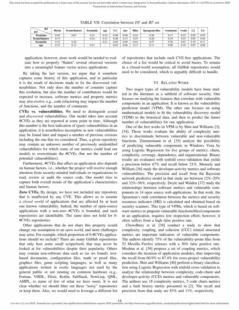
1556-6013 (c) 2018 IEEE. Personal use is permitted, but republication/redistribution requires IEEE permission. See http://www.ieee.org/publications_standards/publications/rights/index.html for more information.
This article has been accepted for publication in a future issue of this journal, but has not been fully edited. Content may change prior to final publication. Citation information: DOI 10.1109/TIFS.2019.2895963, IEEETransactions on Information Forensics and Security
TABLE VII: Correlation between DT and BT setPPPPPDT
BT #forks #contributors #commits age %C size #files #program-files #comment #code L2 L4
#watches 0.95 0.67 0.31 0.12 -0.08 0.08 0.24 0.26 0.17 0.23 0.05 0.03#contributors 0.73 - 0.44 0.13 -0.08 0.13 0.25 0.28 0.19 0.25 0.05 0.04
#commits 0.33 0.44 - 0.21 -0.05 0.69 0.64 0.57 0.56 0.63 0.19 0.11age 0.15 0.13 0.21 - -0.03 0.06 0.13 0.11 0.06 0.10 0.07 0.04
application; however, more work would be needed to eval-uate how to properly “flatten” several observed versionsinto a meaningful feature vector across applications.
By taking the last version, we argue that it somehowcaptures some history of this application, and in particularit is the result of decisions made to fix the discovered vul-nerabilities. Not only does the number of commits capturethis evolution, but also the number of contributors would beexpected to increase, software metrics and property metricsmay also evolve, e.g., code refactoring may impact the numberof functions, and the number of comments.CVEs vs. vulnerabilities. We need to distinguish actualand discovered vulnerabilities. Our model takes into account#CVEs as they are reported at some point in time. Althoughthis number is the best indication of (past) vulnerabilities in anapplication, it is nonetheless incomplete as new vulnerabilitiesmay be found later and impact a number of previous versionsincluding the one that we considered. Thus, a given repositorymay contain an unknown number of previously unidentifiedvulnerabilities for which some of our metrics could lead ourmodels to overestimate the #CVEs (but not the number ofpotential vulnerabilities).
Furthermore, #CVEs that affect an application also dependson human factors, i.e., whether the project will receive enoughattention from security-minded individuals or organizations toread, review or audit the source code. Our model tries tocapture both overall trends of the application’s characteristicsand human factors.Zero CVEs. By design, we have not included any repositorythat is unaffected by any CVE. This allows us to assumea closed world of applications that are affected by at leastone known vulnerability. Indeed, the number of open-sourceapplications with a non-zero #CVEs is bounded, and suchrepositories are identifiable. The same does not hold for 0-#CVEs repositories.
Other applications that do not share this property wouldchange our assumption to an open world, and more challengesmay arise. For example, which proportion of 0-#CVEs applica-tions should we include? There are many GitHub repositoriesthat only host some small scripts/tools that may never belooked at for vulnerabilities despite their popularity. Othersmay contain non-software data such as (as we found): text-based documents, configuration files, math or proof files,graphics files, game scripting languages, as well as manyapplications written in exotic languages not used by thegeneral public or not running on common hardware (e.g.,Fortran, VHDL, Elixir, Kotlin, SaltStack, NewLisp, QML,AMPL, to name of few of what we have seen). It is notclear whether we should filter out these “noisy” repositoriesor keep them. Also, we would need to leverage a different list
of repositories that include such CVE-free applications. Thechoice of a list would be critical to avoid biases. To remainin a closed-world assumption, all GitHub repositories wouldneed to be considered, which is arguably difficult to handle.
VI. RELATED WORK
Two major types of vulnerability models have been stud-ied in the literature as a subfield of software security. Onefocuses on studying the features that correlate with vulnerablecomponents in an application. It is known as the vulnerabilityprediction model (VPM). The other one focuses on usingmathematical models to fit the vulnerability discovery model(VDM) to the historical data, and then to predict the futurenumber of vulnerabilities for one application.
One of the first works in VPM is by Shin and Williams [3],[34]. Those works evaluate the ability of complexity met-rics to discriminate between vulnerable and non-vulnerablefunctions. Zimmermann et al. [35] analyze the possibilityof predicting vulnerable components in Windows Vista byusing Logistic Regression for five groups of metrics: churn,complexity, coverage, dependency, and organizational. Binaryresults are evaluated with tenfold cross-validation that yieldsa precision below 67% and recall below 21%. Meneely andWilliam [36] study the developer-activity metrics and softwarevulnerabilities. The precision and recall from the Bayesiannetwork predictive model in that study are between 12%–29%and 32%–56%, respectively. Doyle and Walden [37] study therelationships between software metrics and vulnerable com-ponents in 14 open source web applications. In that work, theSpearman’s rank correlation between the metrics and securityresources indicator (SRI) is calculated and obtained based onsecurity scanners. This type of VPMs, which is based on soft-ware metrics to pinpoint vulnerable functions/files/componentsin an application, requires low inspection effort; however, itoften suffers from a high false positive rate.
Chowdbury et al. [38] conduct a study to show thatcomplexity, coupling, and cohesion (CCC) related structuralmetrics are important indicators of vulnerable components.The authors identify 75% of the vulnerability-prone files from52 Mozilla Firefox releases with a 30% false positive rate.Moshtar et al. [39] propose a set of coupling metrics, whichconsiders the iteration of application modules, thus improvingthe recall from 60.9% to 87.4% for cross-project vulnerabilityprediction. Shin and Williams [40] perform a binary classifica-tion using Logistic Regression with tenfold cross-validation toanalyze the relationship between complexity, code-churn anddeveloper-activity (CCD) metrics and vulnerable components.The authors use 18 complexity metrics, 5 code churn metricsand a fault history metric presented in [2]. The recall andprecision from that study are 83% and 11%, respectively.
14
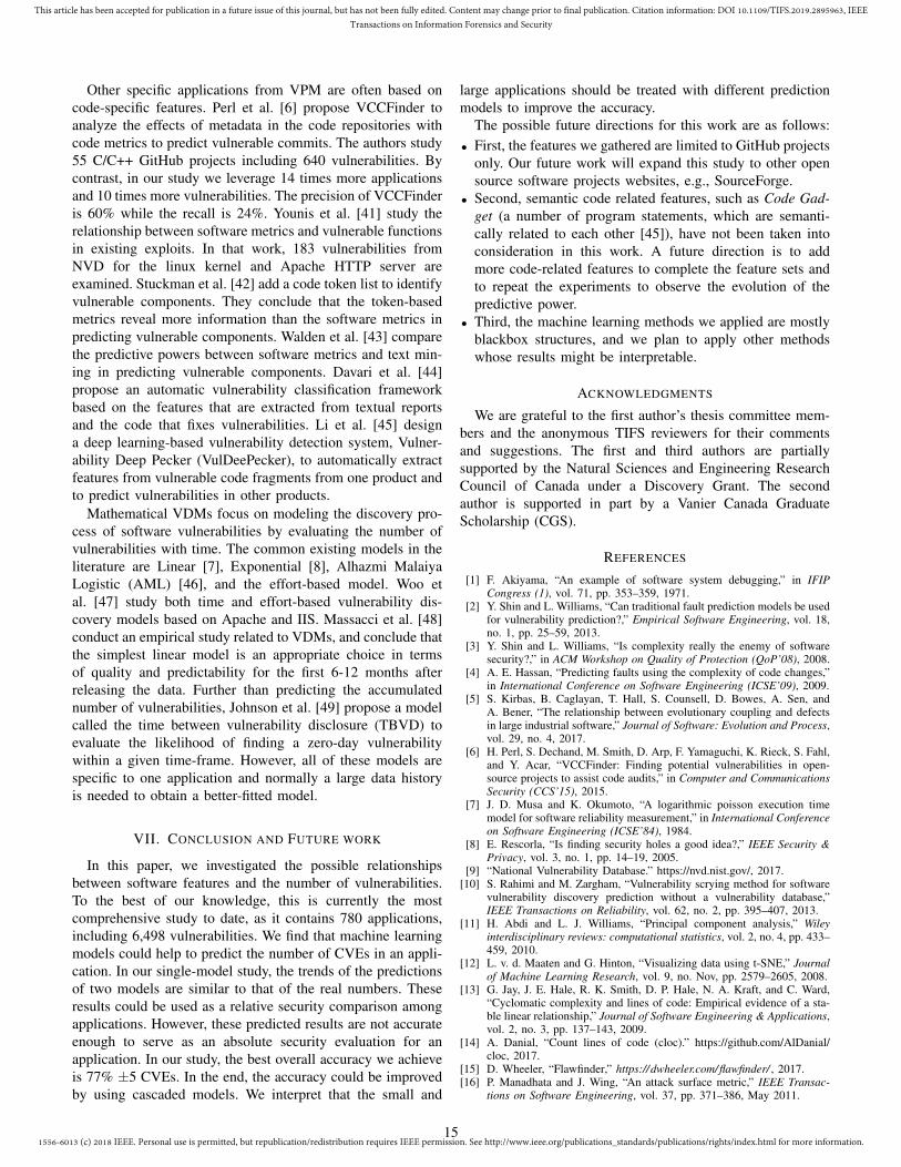
1556-6013 (c) 2018 IEEE. Personal use is permitted, but republication/redistribution requires IEEE permission. See http://www.ieee.org/publications_standards/publications/rights/index.html for more information.
This article has been accepted for publication in a future issue of this journal, but has not been fully edited. Content may change prior to final publication. Citation information: DOI 10.1109/TIFS.2019.2895963, IEEETransactions on Information Forensics and Security
Other specific applications from VPM are often based oncode-specific features. Perl et al. [6] propose VCCFinder toanalyze the effects of metadata in the code repositories withcode metrics to predict vulnerable commits. The authors study55 C/C++ GitHub projects including 640 vulnerabilities. Bycontrast, in our study we leverage 14 times more applicationsand 10 times more vulnerabilities. The precision of VCCFinderis 60% while the recall is 24%. Younis et al. [41] study therelationship between software metrics and vulnerable functionsin existing exploits. In that work, 183 vulnerabilities fromNVD for the linux kernel and Apache HTTP server areexamined. Stuckman et al. [42] add a code token list to identifyvulnerable components. They conclude that the token-basedmetrics reveal more information than the software metrics inpredicting vulnerable components. Walden et al. [43] comparethe predictive powers between software metrics and text min-ing in predicting vulnerable components. Davari et al. [44]propose an automatic vulnerability classification frameworkbased on the features that are extracted from textual reportsand the code that fixes vulnerabilities. Li et al. [45] designa deep learning-based vulnerability detection system, Vulner-ability Deep Pecker (VulDeePecker), to automatically extractfeatures from vulnerable code fragments from one product andto predict vulnerabilities in other products.
Mathematical VDMs focus on modeling the discovery pro-cess of software vulnerabilities by evaluating the number ofvulnerabilities with time. The common existing models in theliterature are Linear [7], Exponential [8], Alhazmi MalaiyaLogistic (AML) [46], and the effort-based model. Woo etal. [47] study both time and effort-based vulnerability dis-covery models based on Apache and IIS. Massacci et al. [48]conduct an empirical study related to VDMs, and conclude thatthe simplest linear model is an appropriate choice in termsof quality and predictability for the first 6-12 months afterreleasing the data. Further than predicting the accumulatednumber of vulnerabilities, Johnson et al. [49] propose a modelcalled the time between vulnerability disclosure (TBVD) toevaluate the likelihood of finding a zero-day vulnerabilitywithin a given time-frame. However, all of these models arespecific to one application and normally a large data historyis needed to obtain a better-fitted model.
VII. CONCLUSION AND FUTURE WORK
In this paper, we investigated the possible relationshipsbetween software features and the number of vulnerabilities.To the best of our knowledge, this is currently the mostcomprehensive study to date, as it contains 780 applications,including 6,498 vulnerabilities. We find that machine learningmodels could help to predict the number of CVEs in an appli-cation. In our single-model study, the trends of the predictionsof two models are similar to that of the real numbers. Theseresults could be used as a relative security comparison amongapplications. However, these predicted results are not accurateenough to serve as an absolute security evaluation for anapplication. In our study, the best overall accuracy we achieveis 77% ±5 CVEs. In the end, the accuracy could be improvedby using cascaded models. We interpret that the small and
large applications should be treated with different predictionmodels to improve the accuracy.
The possible future directions for this work are as follows:• First, the features we gathered are limited to GitHub projects
only. Our future work will expand this study to other opensource software projects websites, e.g., SourceForge.
• Second, semantic code related features, such as Code Gad-get (a number of program statements, which are semanti-cally related to each other [45]), have not been taken intoconsideration in this work. A future direction is to addmore code-related features to complete the feature sets andto repeat the experiments to observe the evolution of thepredictive power.
• Third, the machine learning methods we applied are mostlyblackbox structures, and we plan to apply other methodswhose results might be interpretable.
ACKNOWLEDGMENTS
We are grateful to the first author’s thesis committee mem-bers and the anonymous TIFS reviewers for their commentsand suggestions. The first and third authors are partiallysupported by the Natural Sciences and Engineering ResearchCouncil of Canada under a Discovery Grant. The secondauthor is supported in part by a Vanier Canada GraduateScholarship (CGS).
REFERENCES
[1] F. Akiyama, “An example of software system debugging,” in IFIPCongress (1), vol. 71, pp. 353–359, 1971.
[2] Y. Shin and L. Williams, “Can traditional fault prediction models be usedfor vulnerability prediction?,” Empirical Software Engineering, vol. 18,no. 1, pp. 25–59, 2013.
[3] Y. Shin and L. Williams, “Is complexity really the enemy of softwaresecurity?,” in ACM Workshop on Quality of Protection (QoP’08), 2008.
[4] A. E. Hassan, “Predicting faults using the complexity of code changes,”in International Conference on Software Engineering (ICSE’09), 2009.
[5] S. Kirbas, B. Caglayan, T. Hall, S. Counsell, D. Bowes, A. Sen, andA. Bener, “The relationship between evolutionary coupling and defectsin large industrial software,” Journal of Software: Evolution and Process,vol. 29, no. 4, 2017.
[6] H. Perl, S. Dechand, M. Smith, D. Arp, F. Yamaguchi, K. Rieck, S. Fahl,and Y. Acar, “VCCFinder: Finding potential vulnerabilities in open-source projects to assist code audits,” in Computer and CommunicationsSecurity (CCS’15), 2015.
[7] J. D. Musa and K. Okumoto, “A logarithmic poisson execution timemodel for software reliability measurement,” in International Conferenceon Software Engineering (ICSE’84), 1984.
[8] E. Rescorla, “Is finding security holes a good idea?,” IEEE Security &Privacy, vol. 3, no. 1, pp. 14–19, 2005.
[9] “National Vulnerability Database.” https://nvd.nist.gov/, 2017.[10] S. Rahimi and M. Zargham, “Vulnerability scrying method for software
vulnerability discovery prediction without a vulnerability database,”IEEE Transactions on Reliability, vol. 62, no. 2, pp. 395–407, 2013.
[11] H. Abdi and L. J. Williams, “Principal component analysis,” Wileyinterdisciplinary reviews: computational statistics, vol. 2, no. 4, pp. 433–459, 2010.
[12] L. v. d. Maaten and G. Hinton, “Visualizing data using t-SNE,” Journalof Machine Learning Research, vol. 9, no. Nov, pp. 2579–2605, 2008.
[13] G. Jay, J. E. Hale, R. K. Smith, D. P. Hale, N. A. Kraft, and C. Ward,“Cyclomatic complexity and lines of code: Empirical evidence of a sta-ble linear relationship,” Journal of Software Engineering & Applications,vol. 2, no. 3, pp. 137–143, 2009.
[14] A. Danial, “Count lines of code (cloc).” https://github.com/AlDanial/cloc, 2017.
[15] D. Wheeler, “Flawfinder,” https://dwheeler.com/flawfinder/ , 2017.[16] P. Manadhata and J. Wing, “An attack surface metric,” IEEE Transac-
tions on Software Engineering, vol. 37, pp. 371–386, May 2011.
15
1556-6013 (c) 2018 IEEE. Personal use is permitted, but republication/redistribution requires IEEE permission. See http://www.ieee.org/publications_standards/publications/rights/index.html for more information.
This article has been accepted for publication in a future issue of this journal, but has not been fully edited. Content may change prior to final publication. Citation information: DOI 10.1109/TIFS.2019.2895963, IEEETransactions on Information Forensics and Security
[17] J. Pohjalainen, O. Räsänen, and S. Kadioglu, “Feature selection methodsand their combinations in high-dimensional classification of speakerlikability, intelligibility and personality traits,” Computer Speech &Language, vol. 29, no. 1, pp. 145–171, 2015.
[18] J. Reunanen, “Overfitting in making comparisons between variableselection methods,” Journal of Machine Learning Research, vol. 3,no. Mar, pp. 1371–1382, 2003.
[19] M. A. Hall, Correlation-based feature selection for machine learning.PhD thesis, University of Waikato, Hamilton, New Zealand, Apr. 1999.
[20] R. Battiti, “Using mutual information for selecting features in supervisedneural net learning,” IEEE Transactions on Neural Networks, vol. 5,no. 4, pp. 537–550, 1994.
[21] K. Kira and L. A. Rendell, “The feature selection problem: Traditionalmethods and a new algorithm,” in National Conference on ArtificialIntelligence, vol. 2, pp. 129–134, 1992.
[22] J. Mingers, “An empirical comparison of selection measures fordecision-tree induction,” Machine Learning, vol. 3, no. 4, pp. 319–342,1989.
[23] L. Breiman, “Random forests,” Machine Learning, vol. 45, no. 1, pp. 5–32, 2001.
[24] C. W. Dunnett, “A multiple comparison procedure for comparing severaltreatments with a control,” Journal of the American Statistical Associa-tion, vol. 50, no. 272, pp. 1096–1121, 1955.
[25] C. Vercellis, Business intelligence: data mining and optimization fordecision making. John Wiley & Sons, 2011.
[26] S. Arlot and A. Celisse, “A survey of cross-validation procedures formodel selection,” Statistics Surveys, vol. 4, pp. 40–79, 2010.
[27] MathWorks.com, “Divide data for optimal neural network train-ing.” https://www.mathworks.com/help/nnet/ug/divide-data-for-optimal-neural-network-training.html.
[28] J. W. Sammon, “A nonlinear mapping for data structure analysis,” IEEETransactions on Computers, vol. 100, no. 5, pp. 401–409, 1969.
[29] G. E. Hinton and S. T. Roweis, “Stochastic neighbor embedding,” inAdvances in Neural Information Processing Systems, pp. 857–864, 2003.
[30] L. van der Maaten and G. Hinton, “User’s guide for t-SNE software,”2008. https://lvdmaaten.github.io/tsne/User_guide.pdf.
[31] G. Schryen and R. Kadura, “Open source vs. closed source software:towards measuring security,” in Symposium on Applied Computing(SAC’09), 2009.
[32] Forum of Incident Response and Security Teams, “Vulnerability databasecatalog.” https://www.first.org/global/sigs/vrdx/vdb-catalog.
[33] G. Podjarny, Securing Open Source Libraries. O’Reilly, 2017.[34] Y. Shin and L. Williams, “An empirical model to predict security
vulnerabilities using code complexity metrics,” in Empirical SoftwareEngineering and Measurement (ESEM’08), 2008.
[35] T. Zimmermann, N. Nagappan, and L. Williams, “Searching for aneedle in a haystack: Predicting security vulnerabilities for windowsvista,” in International Conference on Software Testing, Verification andValidation (ICST’10), 2010.
[36] A. Meneely and L. Williams, “Strengthening the empirical analysis ofthe relationship between Linus’ law and software security,” in Interna-tional Symposium on Empirical Software Engineering and Measurement(ESEM’10), 2010.
[37] M. Doyle and J. Walden, “An empirical study of the evolution ofPHP web application security,” in International Workshop on SecurityMeasurements and Metrics (Metrisec), 2011.
[38] I. Chowdhury and M. Zulkernine, “Using complexity, coupling, and co-hesion metrics as early indicators of vulnerabilities,” Journal of SystemsArchitecture - Embedded Systems Design, vol. 57, no. 3, pp. 294–313,2011.
[39] S. Moshtari and A. Sami, “Evaluating and comparing complexity,coupling and a new proposed set of coupling metrics in cross-project vul-nerability prediction,” in Symposium on Applied Computing (SAC’16),2016.
[40] Y. Shin, A. Meneely, L. Williams, and J. A. Osborne, “Evaluatingcomplexity, code churn, and developer activity metrics as indicators ofsoftware vulnerabilities,” IEEE Transactions on Software Engineering,vol. 37, no. 6, pp. 772–787, 2011.
[41] A. Younis, Y. Malaiya, C. Anderson, and I. Ray, “To fear or not to fearthat is the question: Code characteristics of a vulnerable function withan existing exploit,” in Conference on Data and Application Securityand Privacy (CODASPY’16), 2016.
[43] J. Walden, J. Stuckman, and R. Scandariato, “Predicting vulnerable com-ponents: Software metrics vs text mining,” in International Symposiumon Software Reliability Engineering (ISSRE’14), 2014.
[42] J. Stuckman, J. Walden, and R. Scandariato, “The effect of dimen-sionality reduction on software vulnerability prediction models,” IEEETransactions on Reliability, vol. 66, no. 1, pp. 17–37, 2017.
[44] M. Davari, M. Zulkernine, and F. Jaafar, “An automatic softwarevulnerability classification framework,” in International Conference onSoftware Security and Assurance (ICSSA’17), pp. 44–49, IEEE, 2017.
[45] Z. Li, D. Zou, S. Xu, X. Ou, H. Jin, S. Wang, Z. Deng, and Y. Zhong,“VulDeePecker: A deep learning-based system for vulnerability detec-tion,” in Network and Distributed System Security (NDSS’18), 2018.
[46] O. H. Alhazmi and Y. K. Malaiya, “Prediction capabilities of vulner-ability discovery models,” in Annual Reliability and MaintainabilitySymposium (RAMS’06), 2006.
[47] S. Woo, H. Joh, O. H. Alhazmi, and Y. K. Malaiya, “Modeling vulner-ability discovery process in Apache and IIS HTTP servers,” Computers& Security, vol. 30, no. 1, pp. 50–62, 2011.
[48] F. Massacci and V. H. Nguyen, “An empirical methodology to evaluatevulnerability discovery models,” IEEE Transactions on Software Engi-neering, vol. 40, no. 12, pp. 1147–1162, 2014.
[49] P. Johnson, D. Gorton, R. Lagerström, and M. Ekstedt, “Time betweenvulnerability disclosures: A measure of software product vulnerability,”Computers & Security, vol. 62, pp. 278–295, 2016.
Mengyuan Zhang is an Experienced Researcher at EricssonResearch, Montreal, QC, Canada. She received her Ph.D. inInformation and Systems Engineering from Concordia Uni-versity in Montreal. Her research interests include securitymetrics, attack surface and cloud computing security. She haspublished several research papers and book chapters on theaforementioned topics.
Xavier de Carné de Carnavalet is a Ph.D. candidate inInformation and Systems Engineering at Concordia University,Montreal, QC, Canada. He received in 2014 a Dipl.-Ing. fromÉcole Supérieure d’Informatique, Électronique et Automa-tique, Paris, France, and an M.A.Sc. in Information SystemsSecurity from Concordia University. His research interestsare: privacy, passwords and authentication, TLS interception,trusted computing, reverse-engineering, and machine learningapplications to information systems security.
Lingyu Wang is a professor in the Concordia Institutefor Information Systems Engineering (CIISE) at ConcordiaUniversity, Montreal, Quebec, Canada. He received his Ph.D.degree in Information Technology in 2006 from George Ma-son University. He holds a M.E. from Shanghai Jiao TongUniversity and a B.E. from Shenyang Aerospace University inChina. His research interests include cloud computing security,network security metrics, software security, and privacy. Hehas co-authored five books, two patents, and over 100 refereedconference and journal articles at top journals/conferences,such as TOPS, TIFS, TDSC, TMC, JCS, S&P, CCS, NDSS,ESORICS, PETS, ICDT, etc. He is serving as an associateeditor for IEEE Transactions on Dependable and Secure Com-puting (TDSC) and he has served as the program (co)-chairof seven international conferences and the technical programcommittee member of over 100 international conferences.
Ahmed Ragab received the Ph.D. in Industrial Engineer-ing from Polytechnique Montréal, Canada, in 2014. He hasreceived the M.Sc. in Control Engineering in 2007 and theB.Sc. in Electronic Engineering in 2003, from the Faculty ofElectronic Engineering, Menouf, Egypt. His research interestsare: Control Engineering, Machine Learning, Operations Re-search, Discrete Event Systems, Maintenance and ReliabilityEngineering, Fault Diagnosis and Prognosis and DecisionSupport Systems.
16