Embed Size (px)
Citation preview
Lecture #14 - 4/4/2006 Slide 1 of 30
Latent Profile Analysis
Lecture 14April 4, 2006
Clustering and Classification
Overview➤ Today’s Lecture
Latent ProfileAnalysis
MVN
LPA as a FMM
LPA Example #1
Wrapping Up
Lecture #14 - 4/4/2006 Slide 2 of 30
Today’s Lecture
● Latent Profile Analysis (LPA).
● LPA as a specific case of a Finite Mixture Model.
● How to do LPA.
Overview
Latent ProfileAnalysis➤ LPA Input➤ LPA Process➤ LPA Estimation➤ Assumptions
MVN
LPA as a FMM
LPA Example #1
Wrapping Up
Lecture #14 - 4/4/2006 Slide 3 of 30
LPA Introduction
● Latent profile models are commonly attributed to Lazarsfeldand Henry (1968).
● Like K-means and hierarchical clustering techniques, thefinal number of latent classes is not usually predeterminedprior to analysis with latent class models.
✦ The number of classes is determined through comparisonof posterior fit statistics.
✦ The characteristics of each class is also determinedfollowing the analysis.
Overview
Latent ProfileAnalysis➤ LPA Input➤ LPA Process➤ LPA Estimation➤ Assumptions
MVN
LPA as a FMM
LPA Example #1
Wrapping Up
Lecture #14 - 4/4/2006 Slide 4 of 30
Variable Types Used in LPA
● As it was originally conceived, LPA is an analysis that uses:
✦ A set of continuous (metrical) variables - values allowed torange anywhere on the real number line. Examplesinclude:
● The number of classes (an integer ranging from twothrough...) must be specified prior to analysis.
Overview
Latent ProfileAnalysis➤ LPA Input➤ LPA Process➤ LPA Estimation➤ Assumptions
MVN
LPA as a FMM
LPA Example #1
Wrapping Up
Lecture #14 - 4/4/2006 Slide 5 of 30
LPA Process
● For a specified number of classes, LPA attempts to:
✦ For each class, estimate the statistical likelihood of eachvariable.
✦ Estimate the probability that each observation falls intoeach class.
■ For each observation, the sum of these probabilitiesacross classes equals one.
■ This is different from K-means where an observation is amember of a class with certainty.
✦ Across all observations, estimate the probability that anyobservation falls into a class.
Overview
Latent ProfileAnalysis➤ LPA Input➤ LPA Process➤ LPA Estimation➤ Assumptions
MVN
LPA as a FMM
LPA Example #1
Wrapping Up
Lecture #14 - 4/4/2006 Slide 6 of 30
LPA Estimation
● Estimation in LPA is more complicated than in previousmethods discussed in this course.
✦ In agglomerative hierarchical clustering, a search processwas used with new distance matrices being created foreach step.
✦ K-means used more of a brute-force approach - tryingmultiple starting points.
✦ Both methods relied on distance metrics to find clusteringsolutions.
● LPA estimation uses distributional assumptions to findclasses.
● The distributional assumptions provide the measure of"distance" in LPA.
Overview
Latent ProfileAnalysis➤ LPA Input➤ LPA Process➤ LPA Estimation➤ Assumptions
MVN
LPA as a FMM
LPA Example #1
Wrapping Up
Lecture #14 - 4/4/2006 Slide 7 of 30
LPA Distributional Assumptions
● Because LPA works with continuous variables, thedistributional assumptions of LPA must use a continuousdistribution.
● Within each latent class, the variables are assumed to:
✦ Be independent.
✦ (Marginally) be distributed normal (or Gaussian):
■ For a single variable, the normal distribution function is:
f(xi) =1
√
2πσ2x
exp
(−(xi − µx)2
σ2x
)
Overview
Latent ProfileAnalysis
MVN➤ Univariate Review➤ MVN➤ MVN Contours➤ MVN Properties
LPA as a FMM
LPA Example #1
Wrapping Up
Lecture #14 - 4/4/2006 Slide 8 of 30
Joint Distribution
● Because, conditional on class, we have normally distributedvariables in LPA, we could also phrase the likelihood ascoming from a multivariate normal distribution (MVN):
● The next set of slides describes the MVN.
● What you must keep in mind is that our variables are set tobe independent, conditional on class, so the within classcovariance matrix will be diagonal.
Overview
Latent ProfileAnalysis
MVN➤ Univariate Review➤ MVN➤ MVN Contours➤ MVN Properties
LPA as a FMM
LPA Example #1
Wrapping Up
Lecture #14 - 4/4/2006 Slide 9 of 30
Multivariate Normal Distribution
● The generalization of the well-known normal distribution tomultiple variables is called the multivariate normaldistribution (MVN).
● Many multivariate techniques rely on this distribution in somemanner.
● Although real data may never come from a true MVN, theMVN provides a robust approximation, and has many nicemathematical properties.
● Furthermore, because of the central limit theorem, manymultivariate statistics converge to the MVN distribution as thesample size increases.
Overview
Latent ProfileAnalysis
MVN➤ Univariate Review➤ MVN➤ MVN Contours➤ MVN Properties
LPA as a FMM
LPA Example #1
Wrapping Up
Lecture #14 - 4/4/2006 Slide 10 of 30
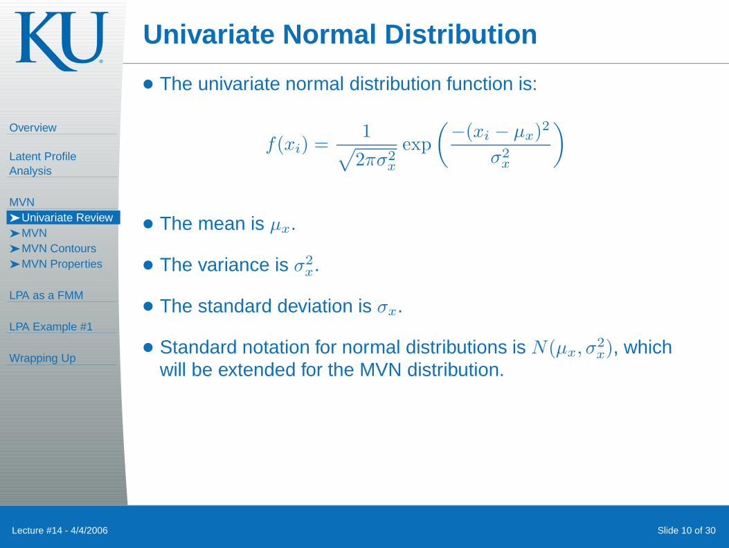
Univariate Normal Distribution
● The univariate normal distribution function is:
f(xi) =1
√
2πσ2x
exp
(−(xi − µx)2
σ2x
)
● The mean is µx.
● The variance is σ2x.
● The standard deviation is σx.
● Standard notation for normal distributions is N(µx, σ2x), which
will be extended for the MVN distribution.
Overview
Latent ProfileAnalysis
MVN➤ Univariate Review➤ MVN➤ MVN Contours➤ MVN Properties
LPA as a FMM
LPA Example #1
Wrapping Up
Lecture #14 - 4/4/2006 Slide 11 of 30
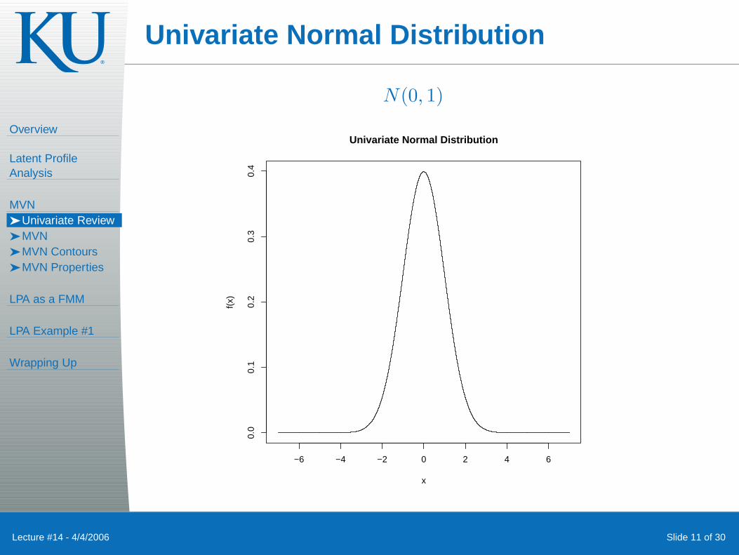
Univariate Normal Distribution
N(0, 1)
−6 −4 −2 0 2 4 6
0.0
0.1
0.2
0.3
0.4
Univariate Normal Distribution
x
f(x)

Overview
Latent ProfileAnalysis
MVN➤ Univariate Review➤ MVN➤ MVN Contours➤ MVN Properties
LPA as a FMM
LPA Example #1
Wrapping Up
Lecture #14 - 4/4/2006 Slide 12 of 30
Univariate Normal Distribution
N(0, 2)
−6 −4 −2 0 2 4 6
0.0
0.1
0.2
0.3
0.4
Univariate Normal Distribution
x
f(x)
Overview
Latent ProfileAnalysis
MVN➤ Univariate Review➤ MVN➤ MVN Contours➤ MVN Properties
LPA as a FMM
LPA Example #1
Wrapping Up
Lecture #14 - 4/4/2006 Slide 13 of 30
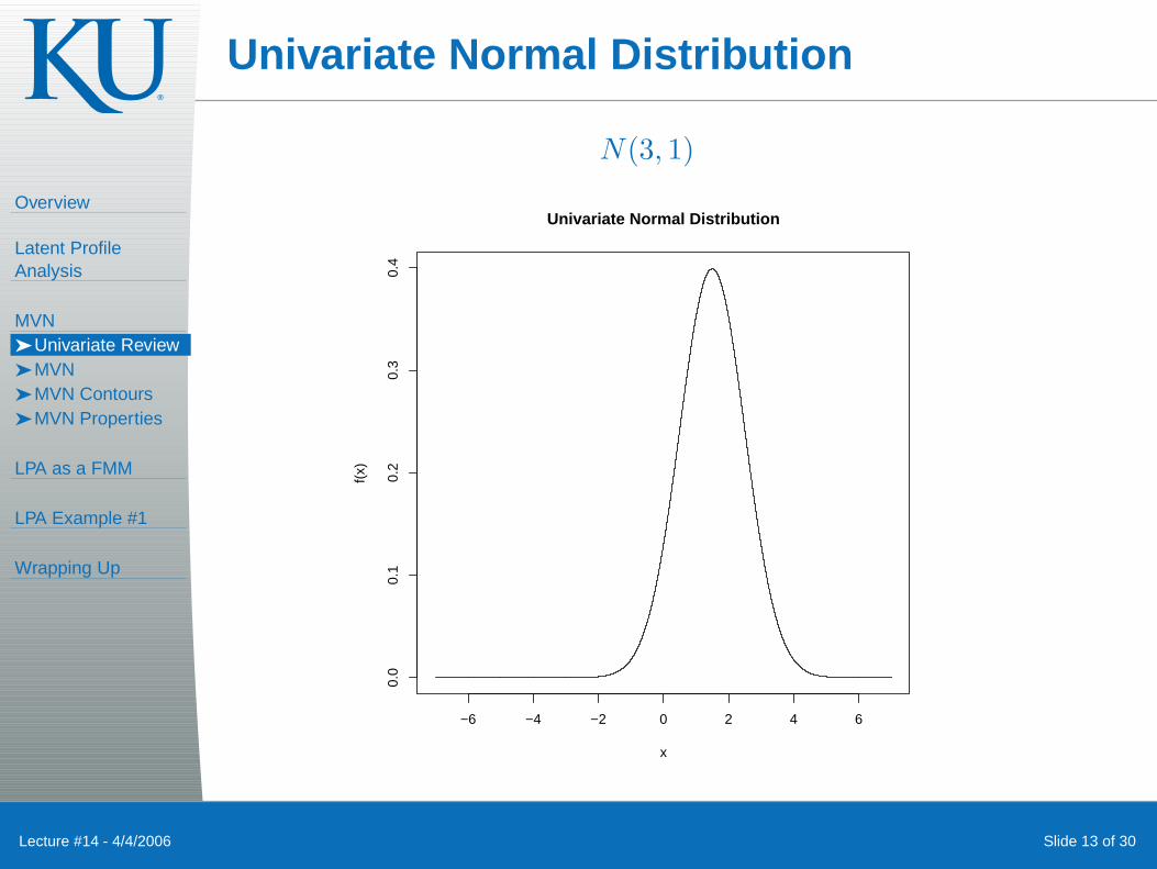
Univariate Normal Distribution
N(3, 1)
−6 −4 −2 0 2 4 6
0.0
0.1
0.2
0.3
0.4
Univariate Normal Distribution
x
f(x)
Overview
Latent ProfileAnalysis
MVN➤ Univariate Review➤ MVN➤ MVN Contours➤ MVN Properties
LPA as a FMM
LPA Example #1
Wrapping Up
Lecture #14 - 4/4/2006 Slide 14 of 30
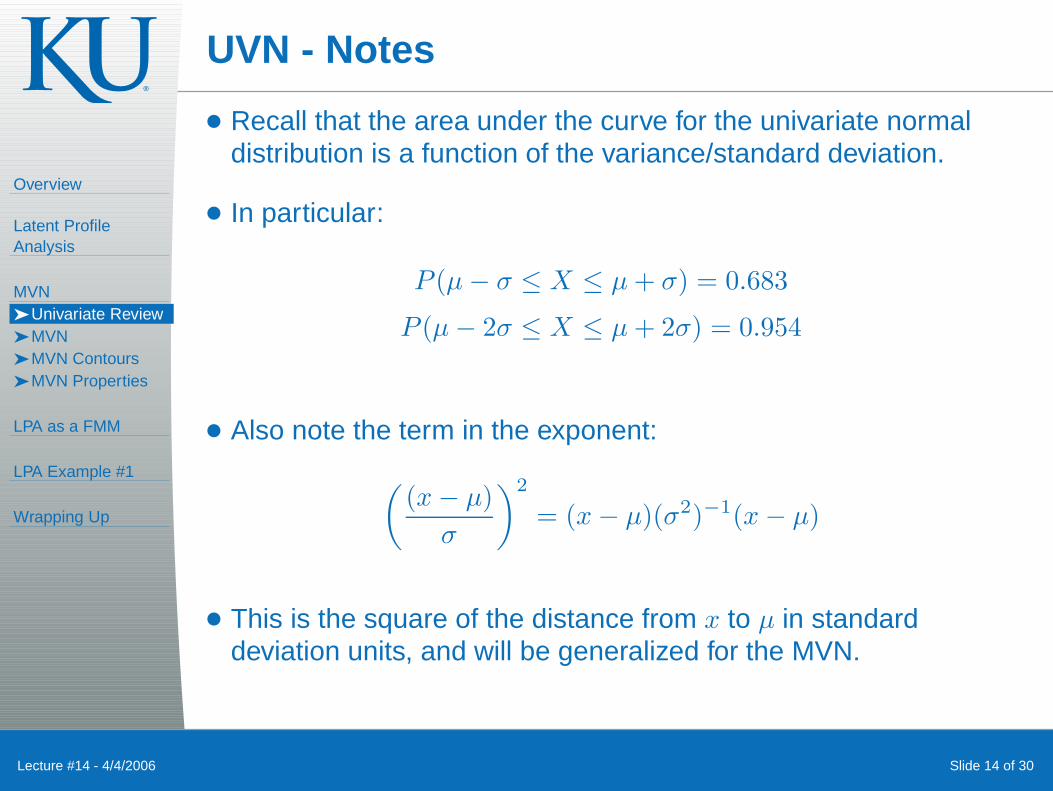
UVN - Notes
● Recall that the area under the curve for the univariate normaldistribution is a function of the variance/standard deviation.
● In particular:
P (µ − σ ≤ X ≤ µ + σ) = 0.683
P (µ − 2σ ≤ X ≤ µ + 2σ) = 0.954
● Also note the term in the exponent:
(
(x − µ)
σ
)2
= (x − µ)(σ2)−1(x − µ)
● This is the square of the distance from x to µ in standarddeviation units, and will be generalized for the MVN.
Overview
Latent ProfileAnalysis
MVN➤ Univariate Review➤ MVN➤ MVN Contours➤ MVN Properties
LPA as a FMM
LPA Example #1
Wrapping Up
Lecture #14 - 4/4/2006 Slide 15 of 30
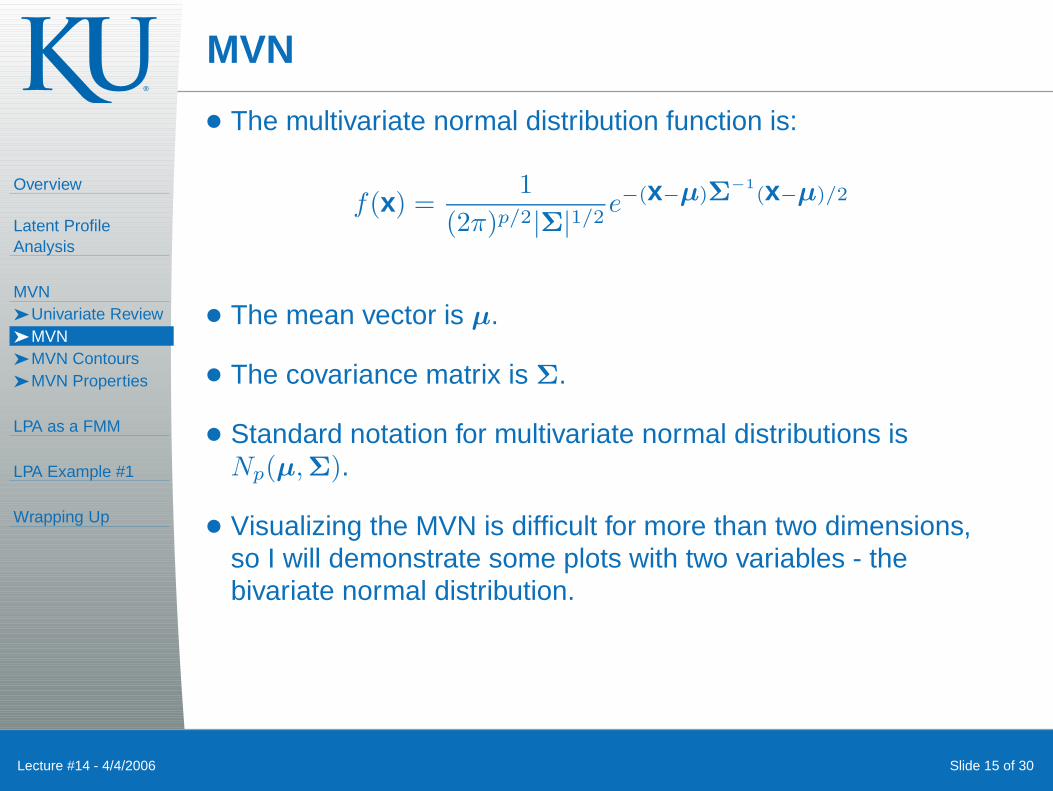
MVN
● The multivariate normal distribution function is:
f(x) =1
(2π)p/2|Σ|1/2e−(x−µ)Σ
−1
(x−µ)/2
● The mean vector is µ.
● The covariance matrix is Σ.
● Standard notation for multivariate normal distributions isNp(µ,Σ).
● Visualizing the MVN is difficult for more than two dimensions,so I will demonstrate some plots with two variables - thebivariate normal distribution.
Overview
Latent ProfileAnalysis
MVN➤ Univariate Review➤ MVN➤ MVN Contours➤ MVN Properties
LPA as a FMM
LPA Example #1
Wrapping Up
Lecture #14 - 4/4/2006 Slide 16 of 30
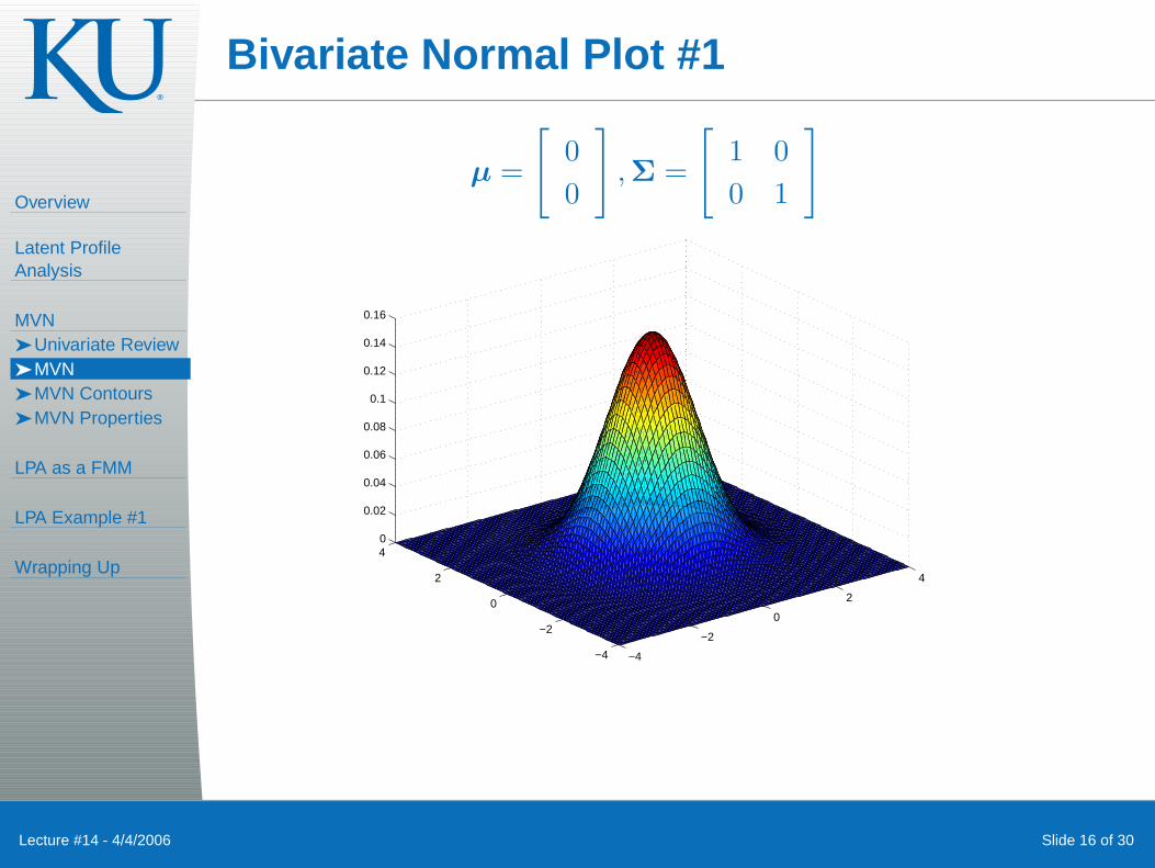
Bivariate Normal Plot #1
µ =
[
0
0
]
,Σ =
[
1 0
0 1
]
−4
−2
0
2
4
−4
−2
0
2
40
0.02
0.04
0.06
0.08
0.1
0.12
0.14
0.16
Overview
Latent ProfileAnalysis
MVN➤ Univariate Review➤ MVN➤ MVN Contours➤ MVN Properties
LPA as a FMM
LPA Example #1
Wrapping Up
Lecture #14 - 4/4/2006 Slide 17 of 30
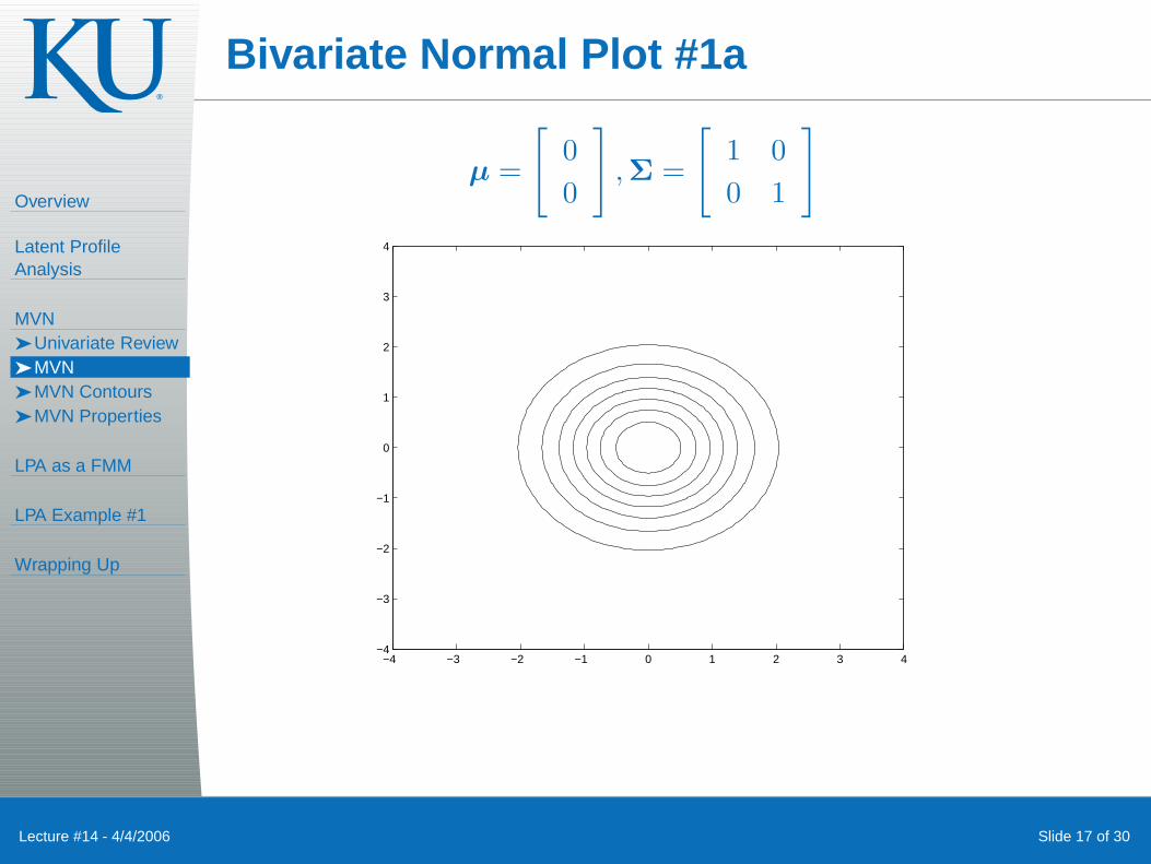
Bivariate Normal Plot #1a
µ =
[
0
0
]
,Σ =
[
1 0
0 1
]
−4 −3 −2 −1 0 1 2 3 4−4
−3
−2
−1
0
1
2
3
4
Overview
Latent ProfileAnalysis
MVN➤ Univariate Review➤ MVN➤ MVN Contours➤ MVN Properties
LPA as a FMM
LPA Example #1
Wrapping Up
Lecture #14 - 4/4/2006 Slide 18 of 30
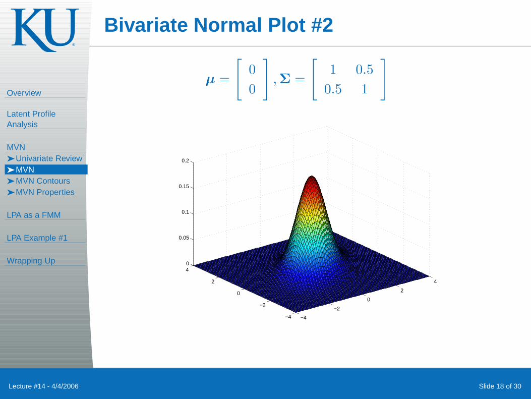
Bivariate Normal Plot #2
µ =
[
0
0
]
,Σ =
[
1 0.5
0.5 1
]
−4
−2
0
2
4
−4
−2
0
2
40
0.05
0.1
0.15
0.2
Overview
Latent ProfileAnalysis
MVN➤ Univariate Review➤ MVN➤ MVN Contours➤ MVN Properties
LPA as a FMM
LPA Example #1
Wrapping Up
Lecture #14 - 4/4/2006 Slide 19 of 30
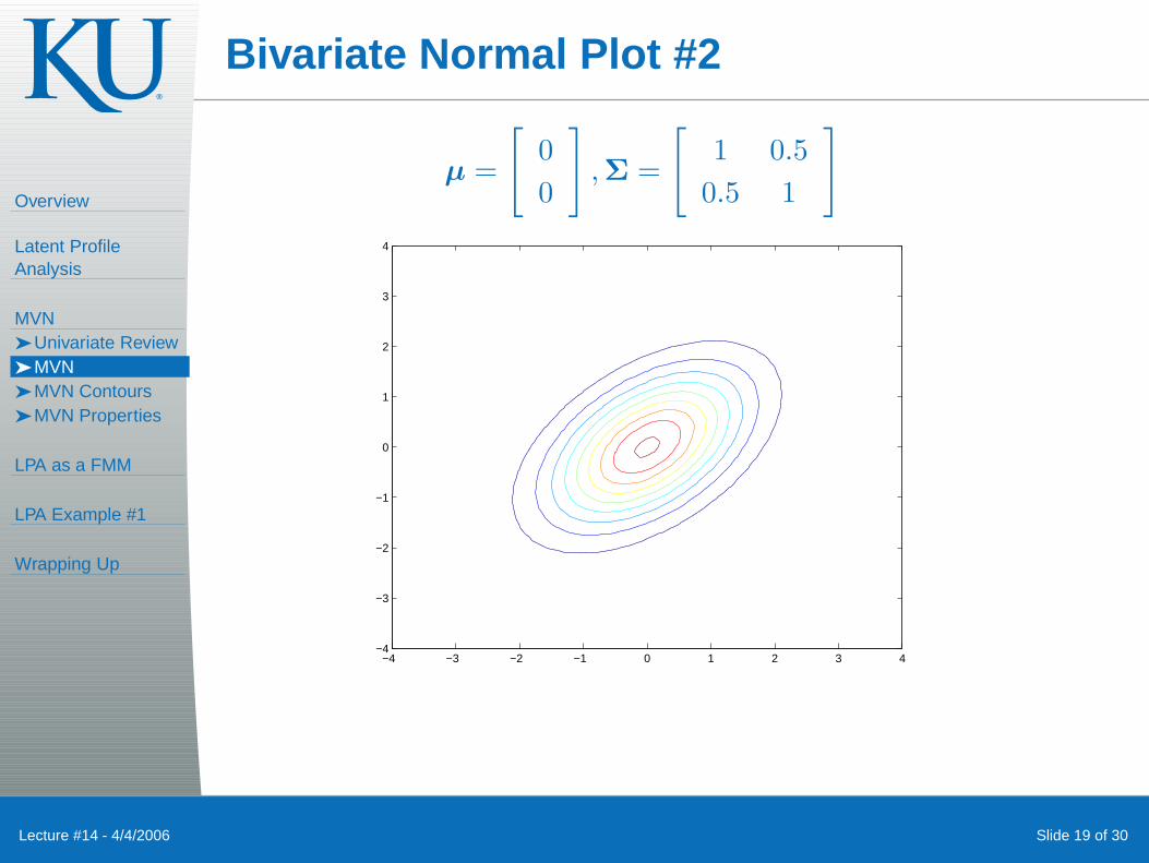
Bivariate Normal Plot #2
µ =
[
0
0
]
,Σ =
[
1 0.5
0.5 1
]
−4 −3 −2 −1 0 1 2 3 4−4
−3
−2
−1
0
1
2
3
4
Overview
Latent ProfileAnalysis
MVN➤ Univariate Review➤ MVN➤ MVN Contours➤ MVN Properties
LPA as a FMM
LPA Example #1
Wrapping Up
Lecture #14 - 4/4/2006 Slide 20 of 30
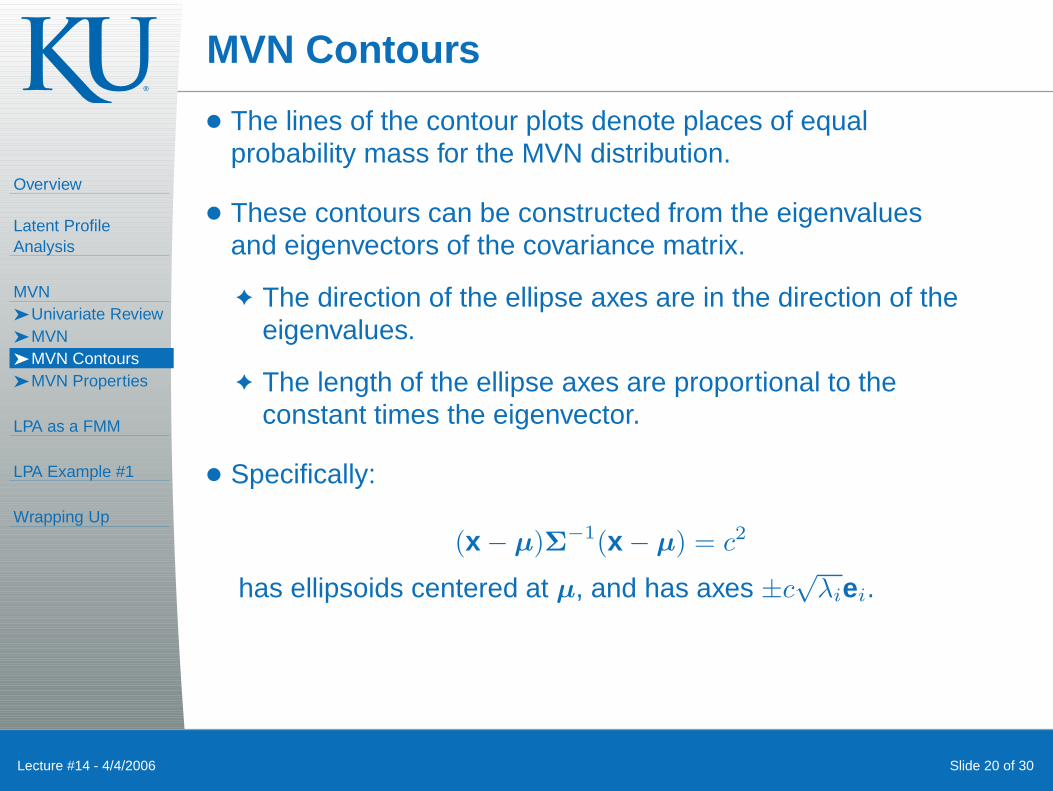
MVN Contours
● The lines of the contour plots denote places of equalprobability mass for the MVN distribution.
● These contours can be constructed from the eigenvaluesand eigenvectors of the covariance matrix.
✦ The direction of the ellipse axes are in the direction of theeigenvalues.
✦ The length of the ellipse axes are proportional to theconstant times the eigenvector.
● Specifically:
(x − µ)Σ−1(x − µ) = c2
has ellipsoids centered at µ, and has axes ±c√
λiei.
Overview
Latent ProfileAnalysis
MVN➤ Univariate Review➤ MVN➤ MVN Contours➤ MVN Properties
LPA as a FMM
LPA Example #1
Wrapping Up
Lecture #14 - 4/4/2006 Slide 21 of 30
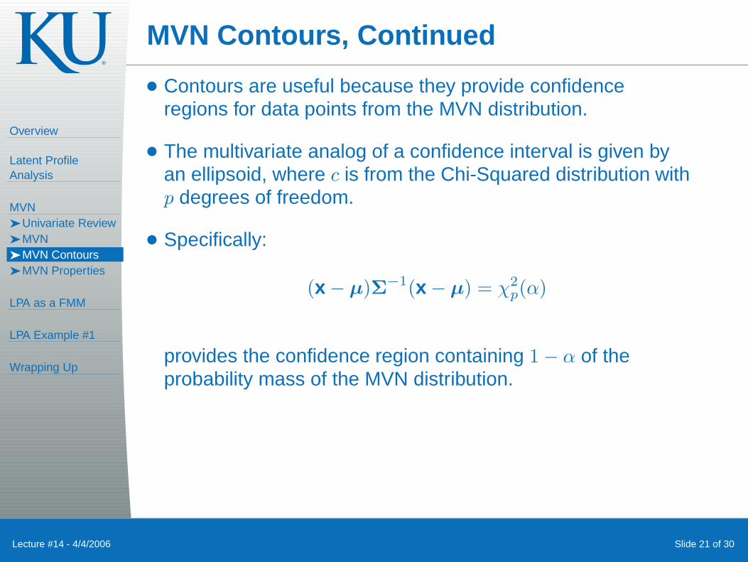
MVN Contours, Continued
● Contours are useful because they provide confidenceregions for data points from the MVN distribution.
● The multivariate analog of a confidence interval is given byan ellipsoid, where c is from the Chi-Squared distribution withp degrees of freedom.
● Specifically:
(x − µ)Σ−1(x − µ) = χ2p(α)
provides the confidence region containing 1 − α of theprobability mass of the MVN distribution.
Overview
Latent ProfileAnalysis
MVN➤ Univariate Review➤ MVN➤ MVN Contours➤ MVN Properties
LPA as a FMM
LPA Example #1
Wrapping Up
Lecture #14 - 4/4/2006 Slide 22 of 30
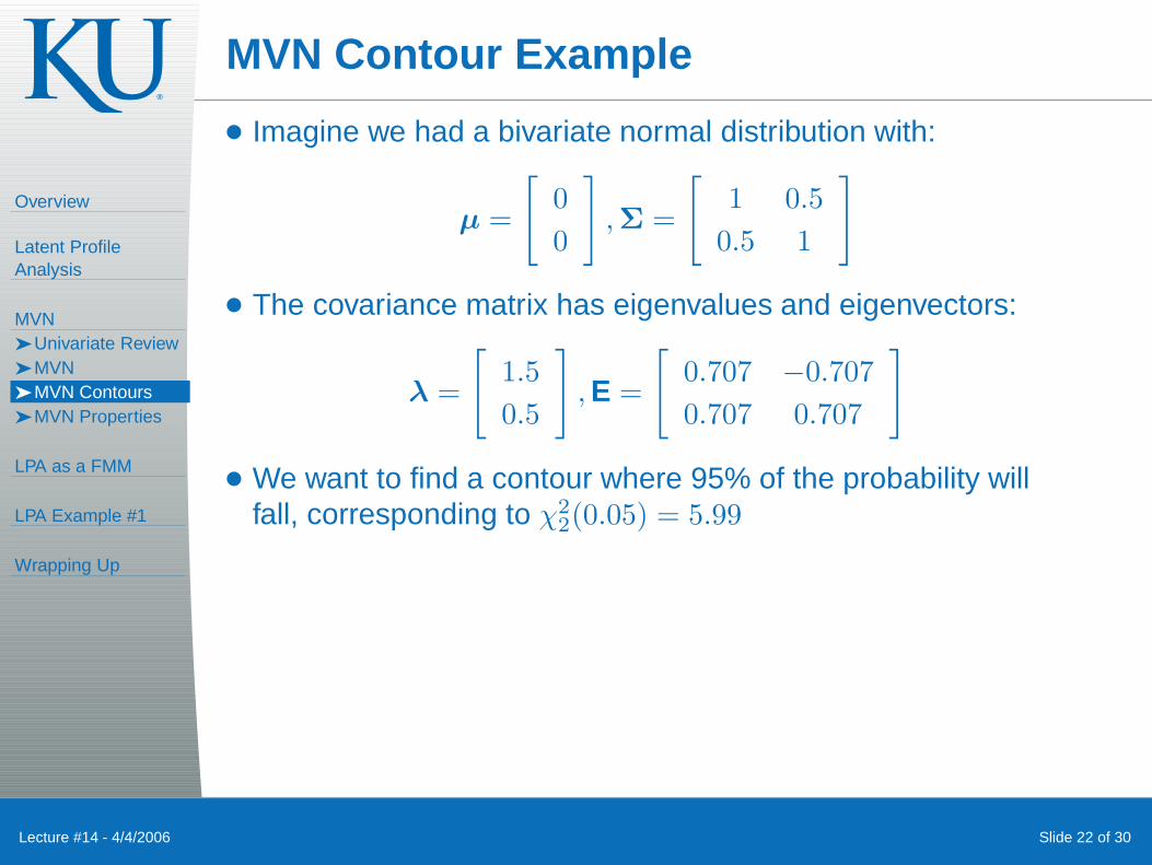
MVN Contour Example
● Imagine we had a bivariate normal distribution with:
µ =
[
0
0
]
,Σ =
[
1 0.5
0.5 1
]
● The covariance matrix has eigenvalues and eigenvectors:
λ =
[
1.5
0.5
]
, E =
[
0.707 −0.707
0.707 0.707
]
● We want to find a contour where 95% of the probability willfall, corresponding to χ2
2(0.05) = 5.99
Overview
Latent ProfileAnalysis
MVN➤ Univariate Review➤ MVN➤ MVN Contours➤ MVN Properties
LPA as a FMM
LPA Example #1
Wrapping Up
Lecture #14 - 4/4/2006 Slide 23 of 30
MVN Contour Example
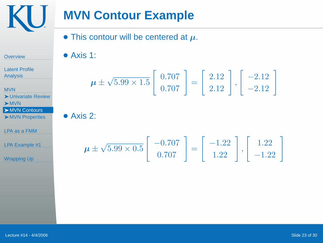
● This contour will be centered at µ.
● Axis 1:
µ ±√
5.99 × 1.5
[
0.707
0.707
]
=
[
2.12
2.12
]
,
[
−2.12
−2.12
]
● Axis 2:
µ ±√
5.99 × 0.5
[
−0.707
0.707
]
=
[
−1.22
1.22
]
,
[
1.22
−1.22
]
Overview
Latent ProfileAnalysis
MVN➤ Univariate Review➤ MVN➤ MVN Contours➤ MVN Properties
LPA as a FMM
LPA Example #1
Wrapping Up
Lecture #14 - 4/4/2006 Slide 24 of 30
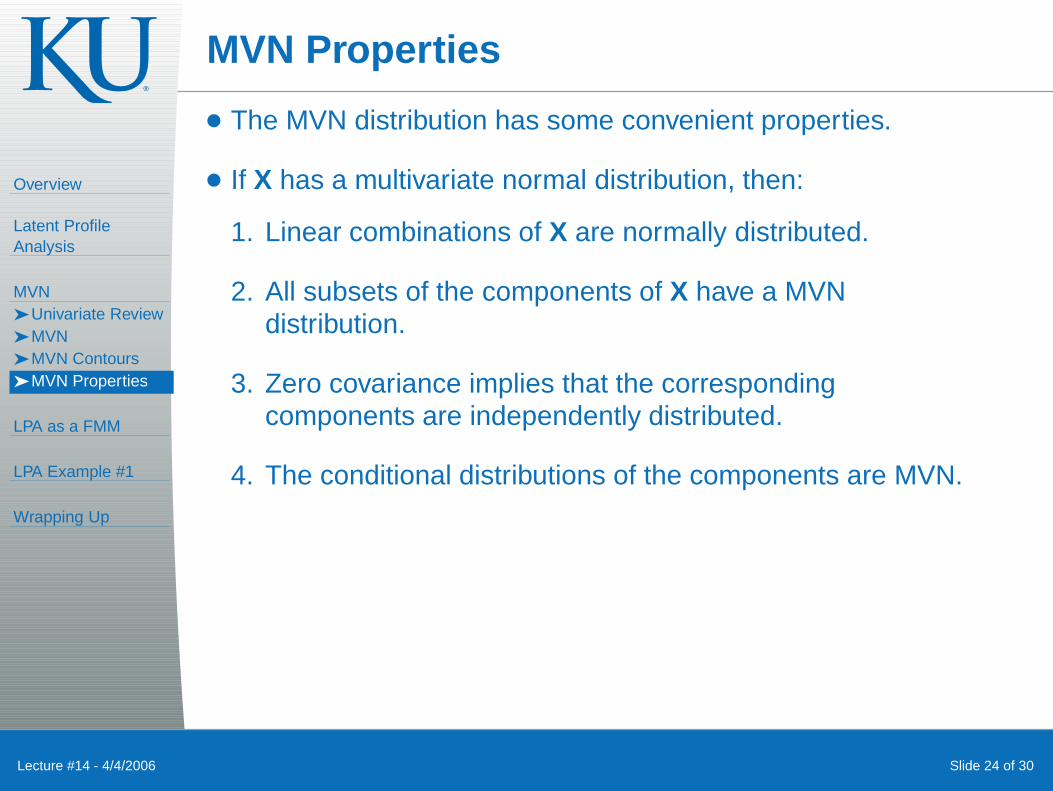
MVN Properties
● The MVN distribution has some convenient properties.
● If X has a multivariate normal distribution, then:
1. Linear combinations of X are normally distributed.
2. All subsets of the components of X have a MVNdistribution.
3. Zero covariance implies that the correspondingcomponents are independently distributed.
4. The conditional distributions of the components are MVN.
Overview
Latent ProfileAnalysis
MVN
LPA as a FMM➤ Finite Mixture
Models➤ LCA as a FMM
LPA Example #1
Wrapping Up
Lecture #14 - 4/4/2006 Slide 25 of 30
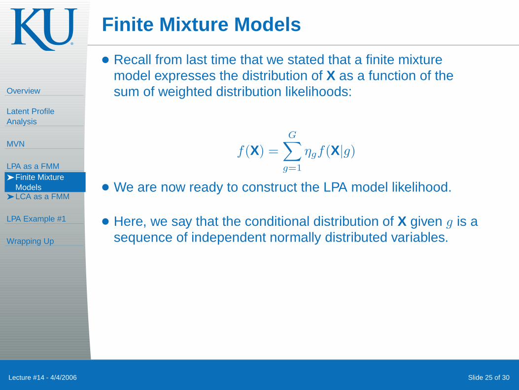
Finite Mixture Models
● Recall from last time that we stated that a finite mixturemodel expresses the distribution of X as a function of thesum of weighted distribution likelihoods:
f(X) =
G∑
g=1
ηgf(X|g)
● We are now ready to construct the LPA model likelihood.
● Here, we say that the conditional distribution of X given g is asequence of independent normally distributed variables.

Overview
Latent ProfileAnalysis
MVN
LPA as a FMM➤ Finite Mixture
Models➤ LCA as a FMM
LPA Example #1
Wrapping Up
Lecture #14 - 4/4/2006 Slide 26 of 30
Latent Class Analysis as a FMM
Using some notation of Bartholomew and Knott, a latent profilemodel for the response vector of p variables (i = 1, . . . , p) withK classes (j = 1, . . . , K):
f(xi) =K∑
j=1
ηj
p∏
i=1
1√
2πσ2ij
exp
(
−(xi − µij)2
σ2ij
)
● ηj is the probability that any individual is a member of class j
(must sum to one).
● xi is the observed response to variable i.
● µij is the mean for variable i for an individual from class j.● σ2
ij is the variance for variable i for an individual from class j.
Overview
Latent ProfileAnalysis
MVN
LPA as a FMM
LPA Example #1➤ Class
Interpretation
Wrapping Up
Lecture #14 - 4/4/2006 Slide 27 of 30
LPA Example
● To illustrate the process of LPA, consider an example usingFisher’s Iris data.
● The Mplus code is found on the next few slides.
● We will use the Plot command to look at our results.
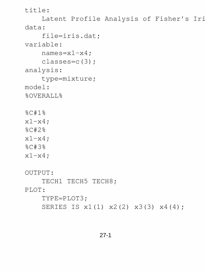
title:Latent Profile Analysis of Fisher’s Iris
data:file=iris.dat;
variable:names=x1-x4;classes=c(3);
analysis:type=mixture;
model:%OVERALL%
%C#1%x1-x4;%C#2%x1-x4;%C#3%x1-x4;
OUTPUT:TECH1 TECH5 TECH8;
PLOT:TYPE=PLOT3;SERIES IS x1(1) x2(2) x3(3) x4(4);
27-1

SAVEDATA:FILE IS myfile.dat;SAVE = CPROBABILITIES;
27-2
Overview
Latent ProfileAnalysis
MVN
LPA as a FMM
LPA Example #1➤ Class
Interpretation
Wrapping Up
Lecture #14 - 4/4/2006 Slide 28 of 30
Interpreting Classes
● After the analysis isfinished, we need toexamine the itemprobabilities to gaininformation about thecharacteristics of theclasses.
● An easy way to do this is tolook at a chart of the itemresponse means by class.
Overview
Latent ProfileAnalysis
MVN
LPA as a FMM
LPA Example #1
Wrapping Up➤ Final Thought➤ Next Class
Lecture #14 - 4/4/2006 Slide 29 of 30
Final Thought
● LPA is a wonderfultechnique to use to findclasses with very specifictypes of data.
● We have only scratched thesurface of LPA techniques.
● We will discuss estimation and other models in the weeks tocome.
Overview
Latent ProfileAnalysis
MVN
LPA as a FMM
LPA Example #1
Wrapping Up➤ Final Thought➤ Next Class
Lecture #14 - 4/4/2006 Slide 30 of 30
Next Time
● No class next two meetings (4-6 and 4-11).
● Our next class:
✦ More LPA examples/facets.
✦ A bit about estimation of such models.